the Creative Commons Attribution 4.0 License.
the Creative Commons Attribution 4.0 License.
 | 16 Apr 2020
On the numerical integration of the Lorenz-96 model, with scalar additive noise, for benchmark twin experiments
Marc Bocquet
Alberto Carrassi
Relatively little attention has been given to the impact of discretization error on twin experiments in the stochastic form of the Lorenz-96 equations when the dynamics are fully resolved but random. We study a simple form of the stochastically forced Lorenz-96 equations that is amenable to higher-order time-discretization schemes in order to investigate these effects. We provide numerical benchmarks for the overall discretization error, in the strong and weak sense, for several commonly used integration schemes and compare these methods for biases introduced into ensemble-based statistics and filtering performance. The distinction between strong and weak convergence of the numerical schemes is focused on, highlighting which of the two concepts is relevant based on the problem at hand. Using the above analysis, we suggest a mathematically consistent framework for the treatment of these discretization errors in ensemble forecasting and data assimilation twin experiments for unbiased and computationally efficient benchmark studies. Pursuant to this, we provide a novel derivation of the order 2.0 strong Taylor scheme for numerically generating the truth twin in the stochastically perturbed Lorenz-96 equations.
- Article
(3455 KB) - Full-text XML
- BibTeX
- EndNote


1.1 Twin experiments with geophysical models
Data assimilation and ensemble-based forecasting have together become the prevailing modes of prediction and uncertainty quantification in geophysical modeling. Data assimilation (DA) broadly refers to techniques used to combine numerical model simulations and real-world observations in order to produce an estimate of a posterior probability density for the modeled state or some statistic of it. In this Bayesian framework, an ensemble-based forecast represents a sampling procedure for the probability density of the forecast prior. The process of sequentially and recursively estimating the distribution for the state of the system by combining model forecasts and streaming observations is known as filtering. Due to the large dimensionality and complexity of operational geophysical models, an accurate representation of the true Bayesian posterior is infeasible. Therefore, DA cycles typically estimate the first two moments of the posterior or its mode – see, e.g, the recent review of DA by Carrassi et al. (2018).
Many simplifying assumptions are used to produce these posterior estimates, and “toy” models are commonly used to assess the accuracy and robustness of approximations made with a DA scheme in a controlled environment. Toy models are small-scale analogues to full-scale geophysical dynamics that are transparent in their design and computationally simple to resolve. In this setting it is possible to run rigorous twin experiments in which artificial observations are generated from a “true” trajectory of the toy model, while ensemble-based forecasts are generated and recalibrated by the observation–analysis–forecast cycle of the DA scheme. Using the known true system state, techniques for state estimation and uncertainty quantification can be assessed objectively under a variety of model and observational configurations. In the case that: (i) a toy model is entirely deterministic; (ii) both the truth twin and model twin are evolved with respect to identical system parameters; and (iii) both the truth twin and model twin are resolved with the same discretization; the only uncertainty in a twin experiment lies in the initialization of the model and the observations of the true state. The model dynamics which generate the ensemble forecast are effectively a “perfect” representation of the true dynamics which generate the observations (Leutbecher and Palmer, 2008).
The development of toy models and twin experiments has greatly influenced the theory of DA and predictability (Ghil, 2018), and the above perfect–deterministic model configuration has largely driven early results. Lorenz's seminal paper showed that a small loss in the numerical precision of the discretization of the governing equations is sufficient to produce a loss of long-term predictability in deterministic, chaotic systems (Lorenz, 1963). Understanding that perturbations to a trajectory, tantamount to numerical noise, could lead to rapid divergence significantly influenced the introduction of ensemble-based forecasting in operational settings (Lewis, 2005). In the perfect–deterministic model setting, the asymptotic filter performance can likewise be understood principally in terms of the dynamical properties of the model. Particularly, the statistics are determined by the ability of the filter to correct for the dynamical instabilities of perturbations along the truth-twin trajectory with respect to the sensitivity of the filter to its observations (Gurumoorthy et al., 2017; Bocquet et al., 2017; Bocquet and Carrassi, 2017; Frank and Zhuk, 2018; Maclean and Van Vleck, 2019; Tranninger et al., 2019).
However, the theory for DA and predictability is increasingly concerned with model errors, as studied in, e.g., the recent works of Kang and Harlim (2012), Mitchell and Gottwald (2012), Gottwald and Harlim (2013), Berry and Harlim (2014), Raanes et al. (2015), Carrassi and Vannitsem (2016), and Raanes et al. (2018). Model deficiencies in terms of physics which is not fully understood or which is poorly represented prove to be difficult to quantify with an ensemble-based forecast and to correct with a standard DA cycle. Indeed, when the model is fundamentally biased, increasing the spatial resolution or numerical precision may not generally improve the accuracy of an ensemble-based forecast. It has recently been shown in a deterministic biased-model setting that the numerical precision of the discretization of the ensemble forecast can be significantly reduced without a major deterioration of the (relative) predictive performance of the DA cycle (Hatfield et al., 2018). In this setting, the model bias overwhelms the errors that are introduced due to precision loss when the model twin is resolved with a low order of accuracy; it may be preferable, thus, to exchange lower-precision numerics for an increased number of samples in the ensemble-based forecast in order to better capture the overall spread.
On the other hand, many aspects of geophysical model uncertainty and variability become tractable in a random and non-autonomous dynamical systems framework, in which certain deficiencies of deterministic models can be mitigated with stochastic forcing (Ghil et al., 2008; Chekroun et al., 2011; Dijkstra, 2013; Franzke et al., 2015; Ghil, 2017; Boers et al., 2017). In this way, the theory of random dynamical systems offers a natural step forward from the perfect–deterministic framework in toy models to the development of a novel theory for predictability and DA. As in the perfect–deterministic setting, the DA cycle has recently been given a dynamics-based interpretation in random models in order to develop new DA methodology (Grudzien et al., 2018a, b). However, unlike the case of the deterministic biased model above, important differences in the statistical properties of model forecasts of stochastic dynamical systems have been observed due to the discretization errors of certain low-order schemes. For example, Frank and Gottwald (2018) develop an order 2.0 Taylor scheme to correct the bias in the drift term induced by the Euler–Maruyama scheme in their study system.
This work similarly studies the effects of the bias on ensemble-based forecasts and the DA cycle due to time-discretization error in twin experiments in the stochastically perturbed Lorenz-96 system. In the following, we perform an intercomparison of several commonly used discretization schemes, studying the path-based convergence properties as well as the convergence in distribution of ensemble-based forecasts. The former (strong convergence) determines the ability of the integration scheme to produce observations of the truth twin consistently with the governing equations; the latter (weak convergence) describes the accuracy of the empirically derived sample statistics of the ensemble-based forecast, approximating the fully resolved evolution of the prior under the Fokker–Planck equations. Using these two criteria, we propose a standard benchmark configuration for the numerical integration of the Lorenz-96 model, with additive noise, for ensemble-based forecasting and DA twin experiments. In doing so, we provide a means to control the bias in benchmark studies intended for environments that have inherent stochasticity in the dynamics but do not fundamentally misrepresent the physical process. This scenario corresponds to, e.g., an ideal, stochastically reduced model for a multiscale dynamical system, as is discussed in the following.
1.2 Stochastic dynamics from multiscale systems
It is a typical (and classical) simplification in filtering literature to represent model error in terms of stochastic forcing in the form of additive or multiplicative noise (Jazwinski, 1970). For many realistic geophysical models, this is actually a reasonable representation of model-reduction errors. Empirically, errors due to coarse-grained simulation in probabilistic forecasting are often ameliorated by stochastic parametrization (Palmer et al., 2005). For example, there is evidence that sub-grid-scale convection in oceanic and atmospheric models cannot be accurately parameterized deterministically in terms of the macro-observables of the system. Deterministic parametrizations can faithfully represent the mean response but typically fail to capture its fast-scale variability and thus lead to an overall misrepresentation of the large-scale variability in the climate system; see e.g., Gottwald et al. (2016) and references therein.
Stochastic parametrizations thus offer a physically intuitive approach to rectify these issues; many realistic physical processes can be considered as noise-perturbed realizations of classical deterministic approximations from which they are modeled. Theoretically, the effect of unresolved scales can furthermore be reduced to additive Gaussian noise in the asymptotic limit of scale separation due to the central limit theorem (Gottwald et al., 2015). Several mathematically rigorous frameworks have been developed to model and simulate the stochastic forcing on the large-scale dynamics, including averaging methods, perturbation methods and combinations of the two – see, e.g., the survey of approaches by Demaeyer and Vannitsem (2018). In this way, it is possible to derive exact reductions of deterministic multiscale systems into coarsely resolved stochastic models.
Mathematically rigorous reductions generally provide an implicit form for the reduced model equations as a mix of deterministic terms, stochastic noise terms and non-Markovian memory terms, all present in the equations of the reduced model. This exact, implicit reduction is derived in, e.g., Mori–Zwanzig formalism. In the asymptotic separation of scales, this formulation reduces to a mean field ordinary differential equation (ODE) system with additive noise, eliminating the memory terms, describing the system consistently with homogenization theory. Additionally, empirically based techniques, such as autoregressive methods, have successfully parameterized model reduction errors (Wilks, 2005; Crommelin and Vanden-Eijnden, 2008). At the state of the art, novel learning techniques are furthermore being developed to construct empirically derived stochastic models that are consistent with mathematical theory for stochastic model reduction, with the goal preserving the underlying model physics (Chorin and Lu, 2015; Vissio and Lucarini, 2018; Cotter et al., 2019).
In this work, we will make a simplifying assumption for the form of the stochasticity, as follows: we take a classical filtering framework in which noise is additive, Gaussian, white-in-time and distributed according to a known scalar covariance matrix. Within the stochastic differential equation (SDE) literature, this is sometimes referred to as scalar additive noise, which is a term we will use hereafter. In principle our results can be extended to the Lorenz-96 system with any form of additive, Gaussian, white-in-time noise, though the version of the Taylor scheme presented in this work depends strongly on the assumption of scalar noise. This scheme is derived from the more general form of the strong order 2.0 Taylor scheme for systems with additive noise (Kloeden and Platen, 2013, p. 359), and other forms of additive noise could be examined. However, we note that the derivations of this scheme will become increasingly complex with, e.g., diagonal or circulant matrices of diffusion coefficients.
Both the truth twin and the model twin will be evolved with respect to the same form for the governing equations but with respect to (almost surely) different noise realizations. Conceptually, this represents a perfect–random model; this corresponds physically to an idealized model for the asymptotic separation of timescales between the fast and slow layers in the two-layer Lorenz-96 model.
1.3 The single-layer Lorenz-96 model with scalar additive noise
The Lorenz-96 model (Lorenz, 1996) is commonly used in DA literature as a toy model for twin experiments; see, e.g., Carrassi et al. (2018, and references therein). This is particularly due to the fact that it (i) is extremely scalable, with the potential to exhibit spatially extended chaos in high dimensions (Herrera et al., 2011); (ii) mimics fundamental features of geophysical fluid dynamics, including conservative convection, external forcing and linear dissipation (Lorenz and Emanuel, 1998); and (iii) can be used in its two-layer form to describe multiscale dynamics, with a layer of fast variables corresponding to atmospheric dynamics, coupled with a slow layer corresponding to oceanic dynamics (Lorenz, 2005). The two-layer form of the Lorenz-96 equations has been of particular interest for developing stochastic parametrizations of sub-grid-scale dynamics (see, e.g., Wilks, 2005; Arnold et al., 2013; Chorin and Lu, 2015; Lu et al., 2017; Vissio and Lucarini, 2018). Likewise, the stochastic reduction in the two-layer model to a one-layer model has been used to demonstrate techniques for adaptive DA designs in the presence of model uncertainty (Pulido et al., 2018).
In the present study, we consider the single-layer form of the Lorenz-96 equations perturbed by additive noise, for which the matrix of diffusion coefficients is a scalar matrix. The classical form for the Lorenz-96 equations (Lorenz, 1996) are defined as , where for each state component ,
such that the components of the vector x are given by the variables xi with periodic boundary conditions, x0=xn, and . The term F in the Lorenz-96 system, Eq. (1), is the forcing parameter that injects energy to the model. With the above definition for the classical Lorenz-96 equations, we define the toy model under our consideration to be
where f is defined as in Eq. (1), In is the n×n identity matrix, W(t) is an n-dimensional Wiener process and is a measurable function of (possibly) time-varying diffusion coefficients. In the remainder of this work, the system in Eq. (2) will be denoted the L96-s model. In contrast to studies in which the objective is to obtain a suitable parametrization of the fast-variable layer of the two-layer Lorenz-96 model and perform a model reduction, we use the L96-s system as a perfect model of the known but random dynamical system of interest. The L96-s model is one particularly simple form for the stochastic Lorenz-96 equations that (i) expresses the essential randomness, (ii) is a commonly used formulation for filter benchmarks in twin experiments and (iii) remains amenable to higher-order integration schemes for stochastic differential equations.
In Appendix A we provide a novel derivation of the strong order 2.0 Taylor method for additive noise (Kloeden and Platen, 2013, p. 359) in the context of the L96-s model. This is a nontrivial derivation of the explicit discretization rule that has not previously appeared in the literature, to the knowledge of the authors. We furthermore evaluate the computational efficiency and rates of convergence for each of the following: (i) Euler–Maruyama/Milstein methods, (ii) the strong order 1.0 Runge–Kutta method and (iii) the strong order 2.0 Taylor rule. In Sect. 2 we briefly outline each of the different discretization schemes and discuss their modes of convergence. In Sect. 3 we provide our numerical benchmarks of each scheme for convergence and for bias introduced into ensemble-based forecasts and the DA cycle. In Sect. 3.4 we provide a discussion of each of the methods and propose a computationally efficient framework for statistically robust twin experiments. Section 4 concludes with a final discussion of results and open questions for future work.
2.1 Modes of convergence for stochastic differential equations
Unlike with deterministic models, even when the initial condition of a stochastic dynamical system is precisely known, the evolution of the state must inherently be understood in a probabilistic sense. This precise initial information represents a Dirac-delta distribution for the prior that is instantaneously spread out due to the unknown realizations of the true noise process. In particular, the solution to the initial value problem is not represented by a single sample path but rather by a distribution derived by the forward evolution with respect to the Fokker–Planck equation. Due to the high numerical complexity of resolving the Fokker–Planck equation in systems with state dimensions greater than 3 (Pichler et al., 2013), a Monte Carlo ensemble-based approach is an appealing alternative and is used to derive empirical statistics of the forward distribution.
However, when the noise realizations are themselves known (as is the case for twin experiments) the path of the delta distribution representing the true system state can be approximately reconstructed using a discretization of the appropriate stochastic calculus. This sample path solution explicitly depends on a particular random outcome, and thereby, we will be interested in criteria for evaluating the discretization error for SDEs that take into account the random variation. For the numerical integration of the L96-s model, we will consider two standard descriptions of the convergence of solutions to the approximate discretized evolution to the continuous-time exact solution – we adapt the definitions from pp. 61–62 of Iacus (2009). In each of the below definitions, we refer to the standard Euclidean norm.
- Definition 1
-
Let xSP(t) be a sample path of an SDE and x(t) be an approximation of xSP(t) based upon a discretization with a maximum time step of Δ. Suppose there exists a Δ0>0 such that for any fixed time horizon T and any ,
where 𝔼 denotes the expectation over all possible realizations of the stochastic process and C is a constant independent of Δ. Then x(t) is said to converge strongly to xSP(t) on the order of γ>0.
We note that in the above definition, x and xSP are both subject to the same outcomes of the random process, and the expectation is taken over all possible outcomes.
Strong convergence is the analogue of the discretization of a non-stochastic trajectory and is used to judge the accuracy (on average) of reconstructing a specific sample path based upon a known realization of a Brownian motion. We may also consider, however, whether a discretization rule is able to accurately represent a statistic of the forward-evolved distribution when estimated over many sample paths with respect to different realizations of Brownian a motion – this is the motivation for weak convergence.
- Definition 2
-
Let xSP(t) be a sample path of an SDE and x(t) be an approximation of xSP(t) based upon a discretization with a maximum time step of Δ. Suppose there exists a Δ0>0 such that for any fixed time horizon T, any 2(γ+1) continuously differentiable function g of at most polynomial growth and any ,
where 𝔼 denotes the expectation over all possible realizations of the stochastic process and C is a constant independent of Δ. Then x(t) is said to converge weakly to xSP(t) on the order of γ>0.
The distinction between strong and weak convergence can be thought of as follows: (i) strong convergence measures the mean of the path-discretization errors over all sample paths, whereas (ii) weak convergence can measure the error when representing the mean of all sample paths from an empirical distribution. When studying the empirical statistics of a stochastic dynamical system or of an ensemble-based forecast, weak convergence is an appropriate criterion for the discretization error. However, when we study the root-mean-square error (RMSE) of a filter in a twin experiment, we assume that we have realizations of an observation process depending on a specific sample path of the governing equations. Therefore, while the accuracy of the ensemble-based forecast may be benchmarked with weak convergence, strong convergence is the appropriate criterion to determine the consistency of the truth twin with the governing equations (Hansen and Penland, 2006).
We will now introduce several commonly studied methods of simulation of stochastic dynamics and discuss their strengths and their weaknesses. To limit the scope of the current work, we will focus only on strong discretization schemes; while a strong discretization scheme will converge in both a strong and weak sense, weak discretizations do not always guarantee convergence in the strong sense. We note here, however, that it may be of interest to study weak discretization schemes solely for the purpose of the efficient generation of ensemble-based forecasts – this may be the subject of a future work and will be discussed further in Sect. 4. We will introduce the discretization rules in a general form whenever appropriate. In this section, however, we will only discuss the strong order 2.0 Taylor scheme in a reduced form derived specifically for the Lorenz-96 system with scalar additive noise (L96-s). A more general formulation for additive noise and its reduction to our model is the content of Appendix A.
2.2 A general form of stochastic differential equations
Consider a generic SDE of the form
where f is a vector-valued map in , W(t) is an n-dimensional Wiener process and S is a matrix-valued map of diffusion coefficients in , equal to a square root of the covariance function of the Gaussian stochastic process S(x,t)W(t). In general, the diffusion coefficients S(x,t) can depend on both the state of the random process and time. We note, however, that in the case of additive noise – when – the derivative of the diffusion coefficients with respect to x is zero and the Itô and Stratonovich drift coefficients are equal, due to the zero adjustment term (Kloeden and Platen, 2013; see p. 109). In the following discussions we will denote xk≜x(tk) and assume that uniform time steps are taken such that .
2.3 Euler–Maruyama and Milstein schemes
The Euler–Maruyama scheme is among the simplest extensions of deterministic integration rules to discretize systems of SDEs such as Eq. (5). Like the standard deterministic order 1.0 Euler scheme, the Euler–Maruyama scheme approximates the evolution of a sample path by a functional relationship expressed by Eq. (5).
Euler–Maruyama:
where the term in Eq. (6a) is the deterministic Euler scheme and the term in Eq. (6b) is the matrix of diffusion coefficients S multiplied by the noise WΔ, a mean zero Gaussian random vector of covariance ΔIn.
The Euler–Maruyama scheme benefits from its simple functional form, adaptability to different types of noise and intuitive representation of the SDE. However, with the Definitions 1 and 2 in mind, it is important to note that Euler–Maruyama generally has a weak order of convergence of 1.0 but a strong order of convergence only of 0.5 (discussed by, e.g., Kloeden and Platen (2013) in Theorem 10.2.2). The loss of one-half order of convergence from the deterministic Euler scheme arises from the differences between deterministic calculus and Itô calculus.
The Milstein scheme includes a correction to the rule in Eq. (6), adjusting the discretization of the stochastic terms to match the first-order Itô–Taylor expansion. In the case that the matrix of diffusion coefficients S(x,t) is diagonal, let us denote the ith diagonal element as Si(x,t); then the Milstein scheme takes the component-wise form.
Milstein scheme for diagonal noise:
for the ith state component, where the partial derivative is evaluated at (xk,tk). This and the general multidimensional form for the Milstein scheme can be found on pp. 345–348 of Kloeden and Platen (2013). We note that, in the case of additive noise, the partial derivatives vanish and the Euler–Maruyama and Milstein schemes are equivalent; thus in our example the Euler–Maruyama scheme achieves a strong order of convergence of 1.0.
Although the Euler–Maruyama scheme is simple to implement, we shall see in the following sections that the cost of achieving mathematically consistent simulations quickly becomes prohibitive. Despite the fact that it achieves both a strong and weak convergence of order 1.0 in the L96-s model, the overall discretization error is significantly higher than even other order 1.0 strong convergence methods – the difference between the Euler–Maruyama scheme and other methods lies in the constant C in the bounds in Definitions 1 and 2.
2.4 Runge–Kutta methods
The convergence issues for the Euler–Maruyama scheme are well understood, and there are many rigorous methods used to overcome its limitations (Kloeden and Platen, 2013, pp. xxiii–xxxvi and references therein). However, general higher-order methods can become quite complex due to (i) the presence of higher-order Itô–Taylor expansions in Itô forms of SDEs and/or (ii) the approximation of multiple Itô or Stratonovich integrals necessary to resolve higher-order schemes. Stochastic Runge–Kutta methods can at least eliminate the higher-order Itô–Taylor expansions, though they do not automatically deal with the issues around multiple stochastic integrals; for a discussion on the limits of higher-order Runge–Kutta schemes see, e.g., Burrage and Burrage (1996, 1998).
Given a system of SDEs as in Eq. (5), the straightforward extension of the classical four-stage Runge–Kutta method, proven by Rüemelin (1982), is given below.
Strong order 1.0 Runge–Kutta:
The straightforward extension of the four-stage Runge–Kutta scheme to stochastic systems in Eq. (8) has the benefits that (i) it is an intuitive extension of the commonly used four-stage deterministic rule, making the implementation simple; (ii) it makes few assumptions about the structure of the governing equations; and (iii) in the small noise limit, the rule will be compatible with the deterministic order 4.0 implementation. However, as a trade-off with generality, by not exploiting the dynamical system structure, the discretization in Eq. (8) has strong order of convergence of 1.0 (Hansen and Penland, 2006). Alternatively, we may consider using, e.g., the strong order 2.0 Runge–Kutta method for scalar additive noise (Kloeden and Platen, 2013, p. 411); the form of the L96-s equations indeed satisfies this condition. However, this is an implicit method, coming with the additional cost of, e.g., Newton–Raphson iterations to solve each step forward. While this is a necessary measure for stiff equations, the L96-s equations do not demand this type of precision.
2.5 Strong order 2.0 Taylor scheme
As a generic out-of-the-box method for numerical simulation, the four-stage Runge–Kutta method in Eq. (8) has many advantages over Euler–Maruyama and is a good choice when the noise is nonadditive or the deterministic part of the system lacks a structure that leads to simplification. On the other hand, the combination of (i) constant and vanishing second derivatives of the Lorenz-96 model, (ii) the rotational symmetry of the system in its spatial index and (iii) the condition of scalar additive noise together allow us to present the strong order 2.0 Taylor rule as follows.
Strong order 2.0 Taylor:
define the constants ρp and αp as
For each step of size Δ,
-
Randomly select the vectors ξ, ζ, η, ϕ, and , independently and identically distributed (iid).
-
Compute the random vectors
-
For ξ, a and b defined as above and for each entry of the random vectors indexed by l and j, define the coefficients
which are used to define the random vectors,
and
Then, in matrix form, the integration rule from time tk to tk+1 is given as
where the term in Eq. (14a) is the deterministic order 2.0 Taylor scheme, the term in Eq. (14b) is the stochastic component of the rule and sk≜s(tk). Deriving this relatively simple form for the strong order 2.0 Taylor rule for the L96-s system is nontrivial and this is explained in detail in Appendix A.
In the following section we will illustrate several numerical benchmarks of each of the methods, describing explicitly their rates of strong and weak convergence. We note that the order 2.0 Taylor scheme takes a very different practical form in the following numerical benchmarks versus in a twin experiment. When simulating a sample path for a twin experiment, one can simply use the steps described above to discretize the trajectory. Particularly, the simulation of a sample path by the above converges to some sample path, consistent with the governing equations. We detail the experimental setup for consistently discretizing a known reference sample path in Appendix B.
3.1 Benchmarks for strong and weak convergence
We begin with benchmarks of strong and weak convergence for each method. Subsequently, we will evaluate the differences in the ensemble-based forecast statistics of each method, as well as biases introduced in DA twin experiments. Using these numerical benchmarks, we will formulate a computationally efficient framework for controlling the discretization errors in twin experiments.
In each of the strong and weak convergence benchmarks we use the same experimental setup. As a matter of computational convenience, we set the system dimension at n=10. This allows us to study the asymptotic filtering statistics, both in number of samples in ensemble-based forecasts as well as in the temporal limit and the number of analyses. We begin by generating a long climatological trajectory of the L96-s model, using the order 2.0 Taylor scheme with a time step of . This solution is spun onto the climatological statistics, using 5×10⁶ integration steps, and subsequently evenly sampled at an interval of δt=2, generating M=500 unique initial conditions. We denote this collection of initial conditions . The parameter s is a fixed diffusion coefficient for Eq. (2), fixed for each experiment with .
For each initial condition vm(s) above, we will generate an ensemble size N=102 of finely discretized reference trajectories. Each member of the ensemble is forward evolved to time T=0.125 such that the evolution is weakly nonlinear in the ensemble dynamics, but each trajectory is fully nonlinear. We also generate an ensemble of N coarsely discretized solutions, defined by each of the (i) Euler–Maruyama, (ii) Runge–Kutta and (iii) Taylor schemes, defined via the same Brownian motion realizations as the fine trajectories.
Suppressing indices, we denote the reference trajectories xSP; these solutions are generated by the Euler–Maruyama scheme as a simple-to-implement benchmark discretization. The reference solutions use a step size defined as . Notice that ΔSP is of order 𝒪(10−7) so that the discretization error of xSP is of order 𝒪(10−7). We take the coarse step sizes as such that the coarse time steps range from order 𝒪(10−2) to 𝒪(10−3). Moreover, each of , and is integer valued for all q. This setup ensures that the Brownian motion realization defined over the coarse time steps, size Δq, can be defined consistently with the finely discretized Brownian motion realization with steps of size ΔSP within the coarsely discretized time interval.
Explicitly, for each initial condition we generate a unique ensemble of N=102 realizations of a 10-dimensional Brownian motion process; each Brownian motion realization, indexed by , is defined by a matrix . Each component of the matrix is drawn iid from N(0,ΔSP) representing the realized Brownian motion over the interval [0,T], discretized with steps of size ΔSP. To obtain the equivalent Brownian motion realizations discretized over the coarse time steps, we take the component-wise sum of the finely discretized Brownian increments in between the coarse steps. For the Euler–Maruyama and Runge–Kutta schemes, this is sufficient to guarantee the consistency of Brownian motion realization over the coarse and fine discretizations. However, there is an additional consideration with the Taylor scheme, which is outlined in Appendix B.
Note that the L96-s model is spatially homogeneous, and the Euclidean norm of its state depends on the dimension of the system n. Therefore, we estimate the strong and weak convergence of the discretization schemes component-wise, independently of the state dimension of the model. Let xi and xj denote the ith and jth component of the vector x∈ℝn respectively. Suppressing indices, for each initial condition vm(s), we approximate the following expected values for an arbitrary component j as follows:
where T=0.125. It is to be understood in the above that, despite the suppressed indices, the difference between the reference solution xSP and the coarsely discretized solution x depends on the same value s for the diffusion, the same initial condition m and the same realized Brownian motion b. Thus the above equations make an approximation of Eq. (15) – strong convergence with the ensemble average root-mean-square error (RMSE) of the coarsely discretized solution versus the reference – and Eq. (16) – weak convergence with the RMSE of the ensemble mean of the coarsely discretized solutions versus the ensemble mean of the reference solutions.
It is known that the ensemble average error on the righthand side of Eqs. (15)–(16) is Gaussian distributed around the true expected value, on the left-hand side, for ensembles of Brownian motions with N>15. Computing these ensemble mean errors over the batch of M=500 different initial conditions, we can compute the sample-based estimate of the expected value (the mean over all batches) and the standard deviation of the batch of realizations in order to compute confidence intervals for the expectation (Kloeden and Platen, 2013; see Sect. 9.3).
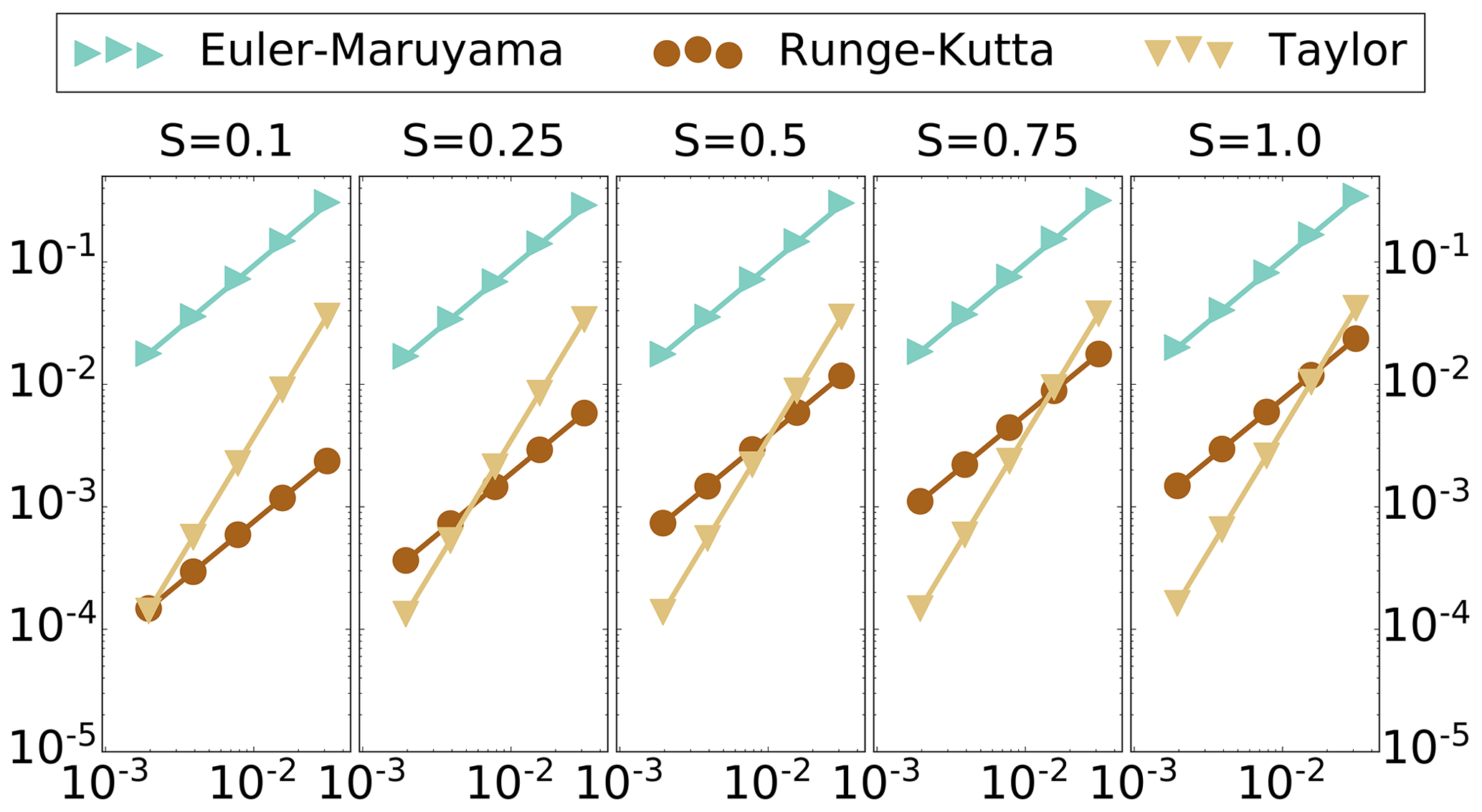
Figure 1Strong convergence benchmark. Vertical axis – discretization error, log scale. Horizontal axis – step size, log scale. Diffusion level s. Length of time T=0.125.
For each coarse discretization, with step size , we compute the point estimate for each expected value on the left-hand side of Eqs. (15)–(16) with the average of the righthand side of Eqs. (15)–(16) taken over the M=500 initial conditions. The average of the righthand side of Eqs. (15)–(16) over all batches will be denoted as the point estimate . Then, within a log–log scale, base 10, we compute the best-fit line between the points using weighted least squares, with weights proportionate to the inverse of the batch standard deviation of the Eqs. (15)–(16). The slope of the line estimated as above is our approximation of the order of convergence γ, and the intercept is the constant C.
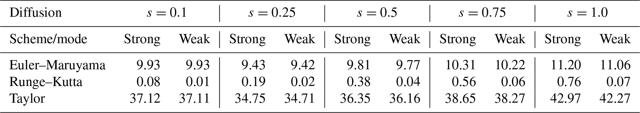
In Fig. 1, we plot the point estimates for the discretization error, measured in strong convergence, for each of the discretization methods: (i) Euler–Maruyama, (ii) Runge–Kutta and (iii) Taylor, as compared with the finely discretized reference solution. It is immediately notable in this plot that, while each order of strong convergence is empirically verified, the lines for Runge–Kutta and Taylor schemes actually cross. Indeed, the estimated slope γ matches the theoretical value within a 10−2 decimal approximation for each scheme (γ=1.0 for each Euler–Maruyama and Runge–Kutta; γ=2.0 for Taylor), but the constants in the order analysis play a major role in the overall discretization error in this system; the Taylor rule has convergence of order 2.0 in the size of the discretization steps, but the constant C associated with the Taylor rule penalizes this scheme heavily, raising the overall discretization error by about an order of magnitude. The constant C for the Runge–Kutta scheme, however, reduces the overall discretization error by about an order of magnitude for each diffusion level (see Table 1).
The effect of this constant C is even more prominent for the case of weak convergence, pictured in Fig. 2. In particular, for the weaker diffusion levels of s=0.1 and 0.25, although the order of weak convergence is 1.0 in the size of discretization step, the order 2.0 Taylor rule fails to achieve a superior discretization error than the Runge–Kutta scheme in this regime. Here, the constant C for the Runge–Kutta scheme is extremely small, lowering the overall order of discretization error by 2 orders of magnitude, despite the order 1.0 weak convergence (see Table 1).
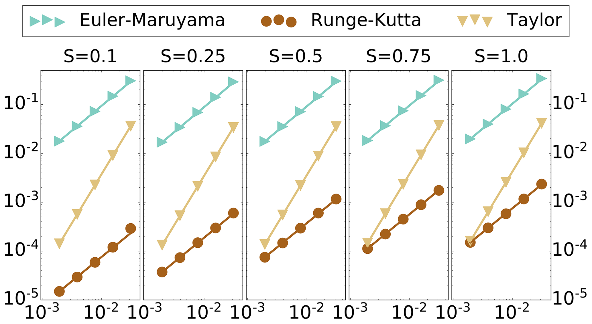
Figure 2Weak convergence benchmark. Vertical axis – discretization error, log scale. Horizontal axis – step size, log scale. Diffusion level s. Length of time T=0.125.
Most interestingly, as the diffusion level s approaches zero, it appears that the behavior of the Runge–Kutta scheme converges in some sense to the four-stage (order 4.0) deterministic Runge–Kutta scheme, but the difference in their orders is reflected in the constant C. Analytically the stochastic Runge–Kutta rule coincides with the deterministic rule in the zero-noise limit. This analytical convergence is also true for the Taylor scheme, where the zero-noise limit is the deterministic Taylor scheme, but the order of convergence for both the stochastic and deterministic Taylor schemes is 2.0, and the overall error does not change so dramatically.
Table 1Estimated discretization error constant C. The constant corresponds to the expected bound of the discretization error, CΔγ, where Δ is the maximum time step of the discretization and is sufficiently small. γ equals 1.0 for Euler–Maruyama and Runge–Kutta and 2.0 for Taylor. Values of C are rounded to 𝒪(10−2).
3.2 Ensemble forecast statistics
The estimated performance of the order 2.0 Taylor scheme using a step size of is of order 𝒪(10−4), in both the strong and weak sense, over all diffusion regimes. Therefore, we will use this configuration as a benchmark setting to evaluate the other methods. While the Runge–Kutta scheme often has better performance than the Taylor scheme in the overall weak-discretization error, the level of discretization error also varies by 1 order of magnitude between different diffusion settings. Therefore, in the following experiments we will consider how the different levels of discretization error and diffusion affect the empirically generated, ensemble-based forecast statistics in the L96-s model with respect to a consistent reference point.
We sample once again the initial conditions as described in Sect. 3.1. For each initial condition, we generate a unique ensemble of N=102 realizations of a 10-dimensional Brownian motion process. Once again, the Brownian motion realizations are indexed by but where each realization is defined by a matrix, . Each component of the matrix is drawn iid from ; this represents a Brownian motion realized over the interval [0,20], discretized at an interval of . For let the matrix be defined as the ensemble matrix. Let the vector be defined as the ensemble mean at time t, averaged over all realized Brownian motions , where the ensemble is generated by the Euler–Maruyama (g=e), Runge–Kutta (g=r) or Taylor (g=t) scheme respectively. Then, for an arbitrary ensemble , we define the spread at time t to be
i.e., defined by the sample-based estimate of the standard deviation of the mean-square deviation of the anomalies (Whitaker and Loughe, 1998).
For each of the Euler–Maruyama and Runge–Kutta schemes , we measure the following: (i) the root-mean-square deviation of the ensemble mean from the benchmark,
and (ii) the ratio of the ensemble spread with that of the benchmark, spreadg(t)∕spreadt(t); each is on an interval of δt=0.01 over the forecast . The integration step size for the Euler–Maruyama and the Runge–Kutta schemes are varied over , and the diffusion level is varied, .
In Figs. 3–4, we plot (i) the median as a solid line, (ii) the inner 80th percentile as a shaded region, and (iii) the minimum and maximum values attained as dashed lines, where each summary statistic is computed over the M=500 initial conditions. In each of the figures we plot the RMSD of the ensemble mean versus the benchmark and the ratio of the ensemble spread only over the interval [0,10]; we find that the statistics are stable in the interval [10,20], and we neglect the longer time series, which remain approximately at the same values as those shown at the end of the pictured time series.
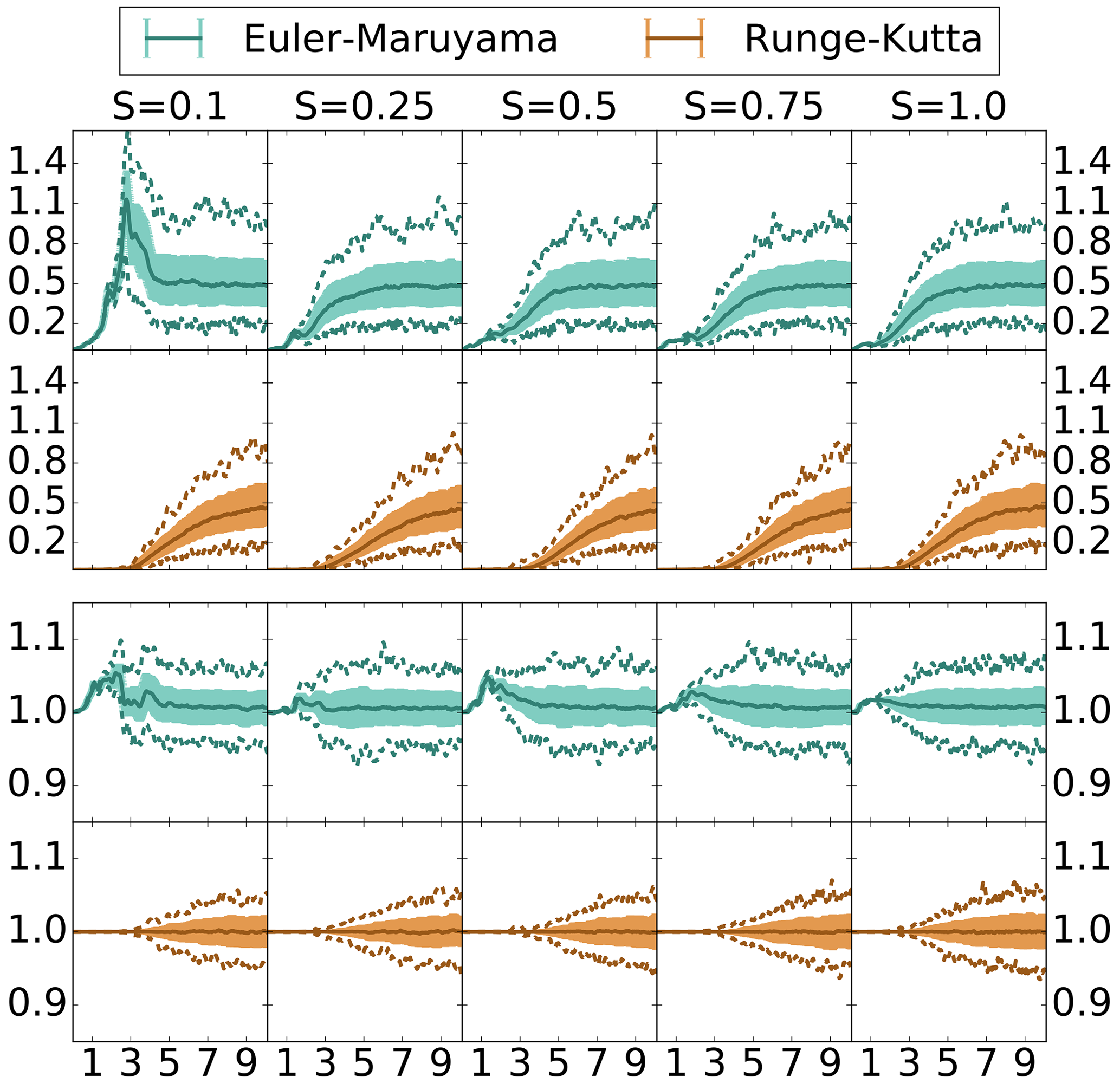
Figure 3Ensemble forecast statistics deviation over time – fine discretization. Euler–Maruyama and Runge–Kutta discretized with time step . Top: RMSD. Bottom: ratio of spread. Median – solid. Inner 80 % – shaded. Min/max – dashed.
In Fig. 3 we note immediately that there are no major differences between the ensemble mean or spread of the finely discretized Runge–Kutta scheme and the benchmark Taylor scheme for forecasts up to length . Indeed, in all diffusion regimes, the RMSD of the ensemble means is bounded by 0.11 for forecasts up to length T=3 and below 0.1 for forecasts up to length T=2.8. In the higher-diffusion regimes, in which the weak-discretization error of the Runge–Kutta scheme becomes slightly higher than the benchmark system, we notice a slight change in the performance in which the ensemble means begin to deviate earlier; however, the difference occurs well beyond what would be considered a practical upper limit of a forecast length, around T=2. Asymptotically as the forecast length T→∞, the RMSD of the means settles to small variations around the median value of 0.5, indicating that by T=10 the Runge–Kutta and benchmark Taylor ensembles have become close to their climatological distributions. This is indicated likewise by the ratio of the ensemble spreads where, beyond T=10, the width of the percentiles around the median ratio, at 1.0, becomes steady.
The relatively slow divergence of the ensembles under Runge–Kutta and Taylor discretizations, finally reaching similar climatological distributions, stands in contrast to the ensemble statistics of the Euler–Maruyama scheme. Notably, the ensemble mean of the Euler–Maruyama scheme quickly diverges. Moreover, at low-diffusion values, the short-timescale divergence is also consistently greater than the deviation of the climatological means. This indicates that, unlike with the Runge–Kutta scheme, a strong bias is present in the empirical forecast statistics with respect to the Euler–Maruyama scheme. The ensemble-based climatological mean generated with the Euler–Maruyama scheme is similar to that under the Taylor scheme; however, the spread of the climatological statistics is consistently greater than that of the benchmark system. After the short period of divergence, the median ratio of the spread of the Euler–Maruyama ensemble versus the Taylor ensemble is actually consistently above 1.0.
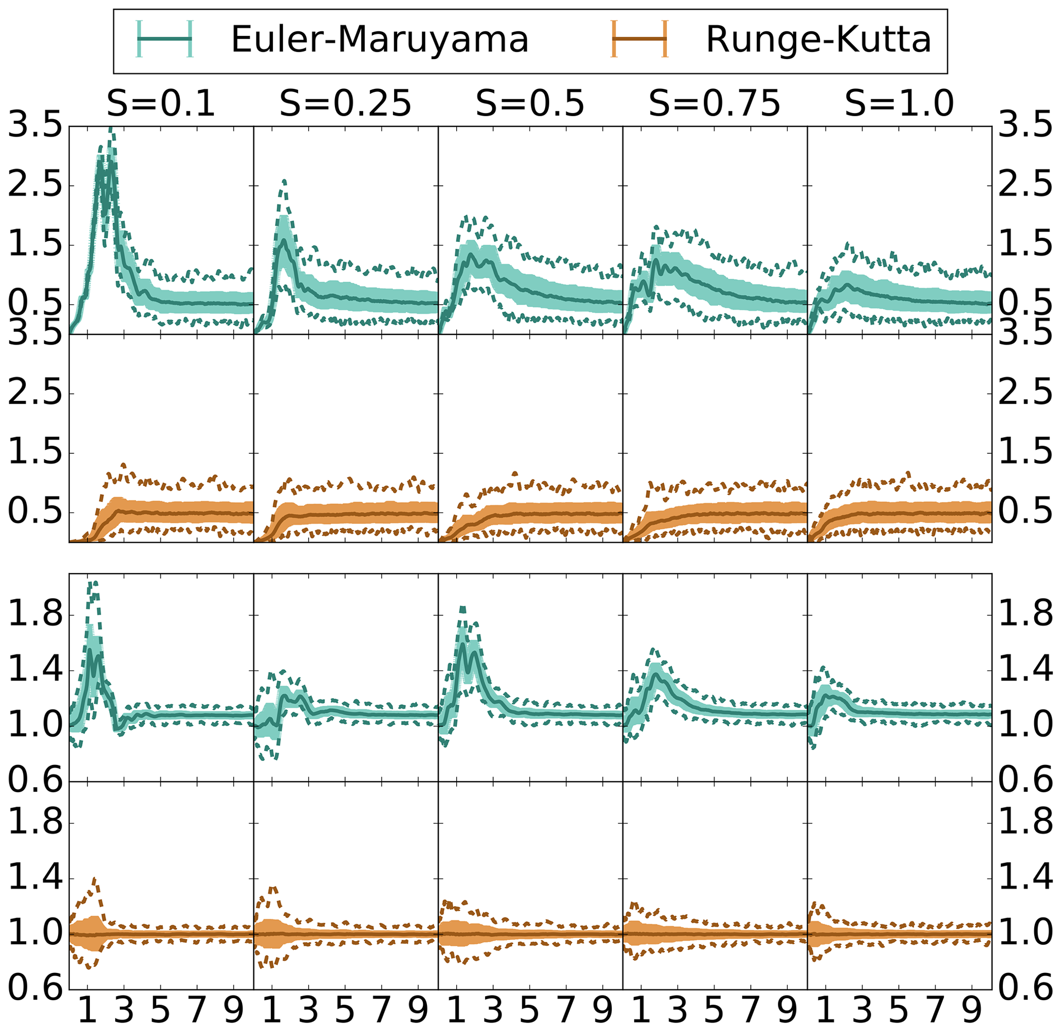
Figure 4Ensemble forecast statistics deviation over time – coarse discretization. Euler–Maruyama and Runge–Kutta discretized with time step . Top: RMSD. Bottom: ratio of spread. Median – solid. Inner 80 % – shaded. Min/max – dashed.
Increasing the step size of the Euler–Maruyama and Runge–Kutta ensembles to , we see in Fig. 4 some similar patterns and some differences. With the large step size the divergence of the ensemble means has a faster onset. However, particularly for the Euler–Maruyama scheme we see the presence of a bias, indicated by the large short-timescale deviation, substantially greater than the climatological deviation of means. For both the Euler–Maruyama and the Runge–Kutta scheme, increased diffusion shortens the initial period of the divergence of the ensemble means, bringing each ensemble closer to the climatological statistics more rapidly. With the increased discretization error, the Runge–Kutta scheme has more variability in its ensemble spread but remains unbiased with the median ratio of spreads centered at one. For the Euler–Maruyama scheme, however, we see the artificial increase in the ensemble spread is even more pronounced, with the minimum value for the ratio of spreads generally exceeding 1.0.
Given the above results, we can surmise that the Runge–Kutta scheme will be largely unbiased in producing ensemble-based forecast statistics, with maximum time discretization of . At the upper endpoint of this interval, divergence of the means occurs more rapidly, and there is more variation in the ensemble spread versus a finer step size. However, the result is that it settles more quickly onto the climatological statistics, close to the benchmark Taylor system. The short-term and climatological statistics of the Euler–Maruyama scheme, however, suffer from biases especially in low-diffusion regimes or for a maximal time discretization of order 𝒪(10−2). In the following section, we will explore how these observed differences in ensemble-based statistics of these schemes affect the asymptotic filtering statistics.
3.3 Data assimilation twin experiments
Here we study the RMSE and the spread of the analysis ensemble of a simple stochastic (perturbed observation) ensemble Kalman filter (EnKF) (Evensen, 2003). We fix the number of ensemble members at N=100 and set the L96-s system state to be fully observed (with Gaussian noise) for all experiments such that no additional techniques are necessary to ensure filter stability for the benchmark system. Particularly, in this configuration, neither inflation nor localization is necessary to ensure stability – this is preferable because inflation and localization techniques typically require some form of tuning of parameters to overcome the usual rank deficiency, the associated spurious correlations and the over confidence in the ensemble-based covariance estimates (Carrassi et al., 2018). The benchmark system uses the order 2.0 Taylor scheme with a time discretization of (i) the truth twin with and (ii) the ensemble with .
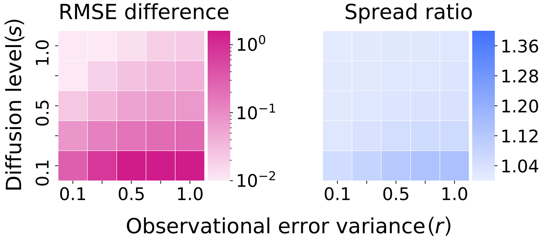
In Fig. 5, we plot the asymptotic-average EnKF analysis RMSE and ensemble spread for our benchmark system over a range of diffusion levels s and a range of observational error variance r, where . The analysis RMSE of the filter is evaluated in terms of the analysis ensemble mean estimate versus the truth twin, with observations given at length T=0.1 between analyses. The average RMSE and spread are calculated over 2.5×10⁴ analysis cycles, with an initial 5×10³ analysis cycles precomputed, not contributing to the average, as a spin-up for the filter to reach its stable statistics. We see, in all combinations of the model and observational error parameters, that the filter is performing well when compared with the standard deviation of the observation errors. The spread also consistently has comparable values to the RMSE, indicating that the performance of the EnKF is stable in this regime (Whitaker and Loughe, 1998).
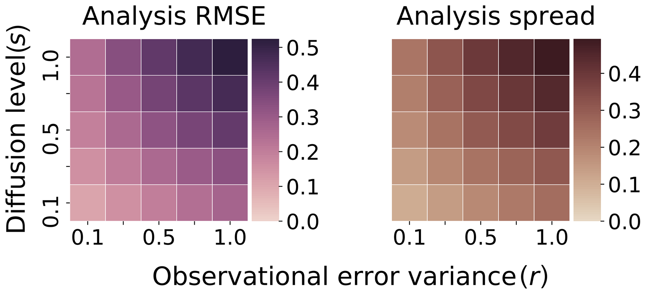
Figure 5Truth: Taylor . Ensemble: Taylor . Asymptotic-average analysis for ensemble RMSE and spread of benchmark configuration. Vertical axis – level of diffusion . Horizontal axis – variance of observation error .
3.3.1 Varying the ensemble integration method for data assimilation
In this section, we will compare several different DA twin experiment configurations with the benchmark system, in which the Taylor scheme generates the truth twin and model forecast with a fine time step. The configuration which is compared to the benchmark system will be referred to as the “test” system. We fix the truth twin to be generated in all cases by the order 2.0 Taylor scheme, with time step . We will vary, on the other hand, the method of generating the forecast ensemble for the test system with different choices of discretization schemes and the associated time step. For each choice of ensemble integration scheme, we once again compute the asymptotic-average analysis RMSE and spread over 2.5×10⁴ analyses, with a 5×10³ analysis spin-up so as to reach stable statistics.
We drop the phrase “asymptotic-average analysis” in the remaining portions of Sect. 3 and instead refer to these simply as the RMSE and spread. In each of the following figures, we plot (i) the RMSE of the EnKF generated in the test system, minus the RMSE of the benchmark system; (ii) the ratio of the spread of the EnKF generated with the test system compared with that of the benchmark configuration. All filters are supplied identical Brownian motion realizations for the model errors, which are used to propagate the ensemble members with their associated integration schemes. Likewise, identical observations (including randomly generated errors) and observation perturbations in the stochastic EnKF analysis are used for each filter at corresponding analysis times.
As was suggested by the results in Sect. 3.2, the difference between the RMSE and the ratio of the spreads for the configuration in which the ensemble is generated by the Runge–Kutta scheme with step size and the benchmark DA configuration is nominal; the RMSE difference is of order 𝒪(10−6), with a mean value and standard deviation of order 𝒪(10−7) across the configurations; the ratio of the spread differs from 1.0 by an order of 𝒪(10−6), with a mean value of order 𝒪(10−6) and a standard deviation of order 𝒪(10−7). For these reasons, we do not plot the comparison of the ensemble generated with the Runge–Kutta scheme with step size and the benchmark configuration. The next question is whether increasing the time step of the Runge–Kutta scheme to will impact the filter performance, especially in terms of causing bias in the results of the filter.
In Fig. 6, the test system uses the Runge–Kutta scheme with coarse time step . We find what appears to be small, random variation in the difference, where in some cases the coarse time step scheme slightly outperforms the benchmark system in terms of the RMSE. These RMSE differences, however, appear to be effectively unstructured in sign or magnitude with regard to the diffusion level s and the observational error variance r, indicating that this amounts to random numerical fluctuation and is mostly unbiased; this is likewise the case for the ratio of the spread.
To formalize the visual inspection, we perform the Shapiro–Wilk test (Shapiro and Wilk, 1965) on the standardized RMSE differences. The result of the Shapiro–Wilk test is a p value of approximately 0.80 so that we fail to reject the null of Gaussian-distributed differences in the RMSE. Assuming that these differences are Gaussian distributed, we apply the t test with null hypothesis that the residuals have a mean of 0. The result is a p value of approximately 0.77, so that we fail to reject the null hypothesis that the differences are distributed according to a mean zero Gaussian distribution.
The average of these RMSE differences is approximately , with a standard deviation of approximately 10−3; the ratio of spreads differs from 1.0 on average by about with a standard deviation of approximately . Because this appears to be unbiased, Gaussian numerical error, we expect that increasing the integration time step for the Runge–Kutta scheme to will not introduce any structural biases to twin experiments based on the discretization error.
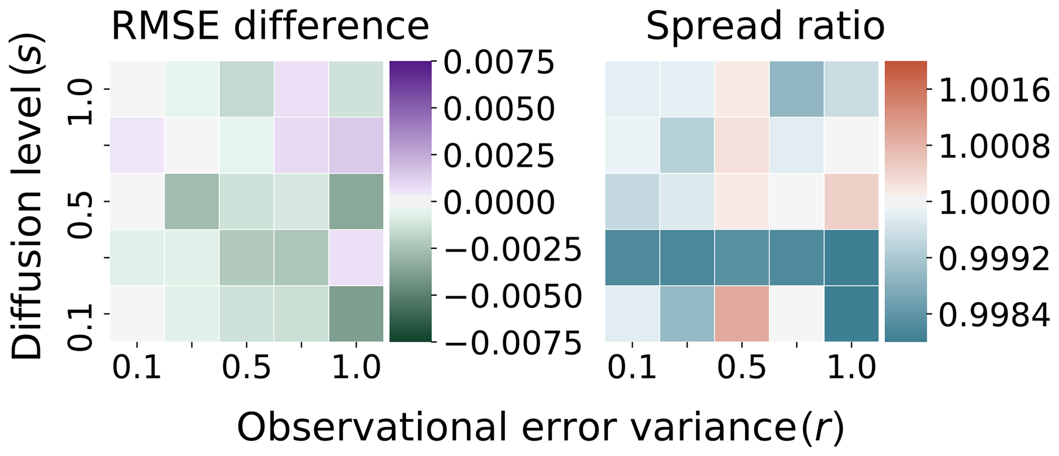
Figure 6Truth: Taylor . Ensemble: Runge–Kutta . Difference in RMSE/ratio spread with benchmark Fig. 5.
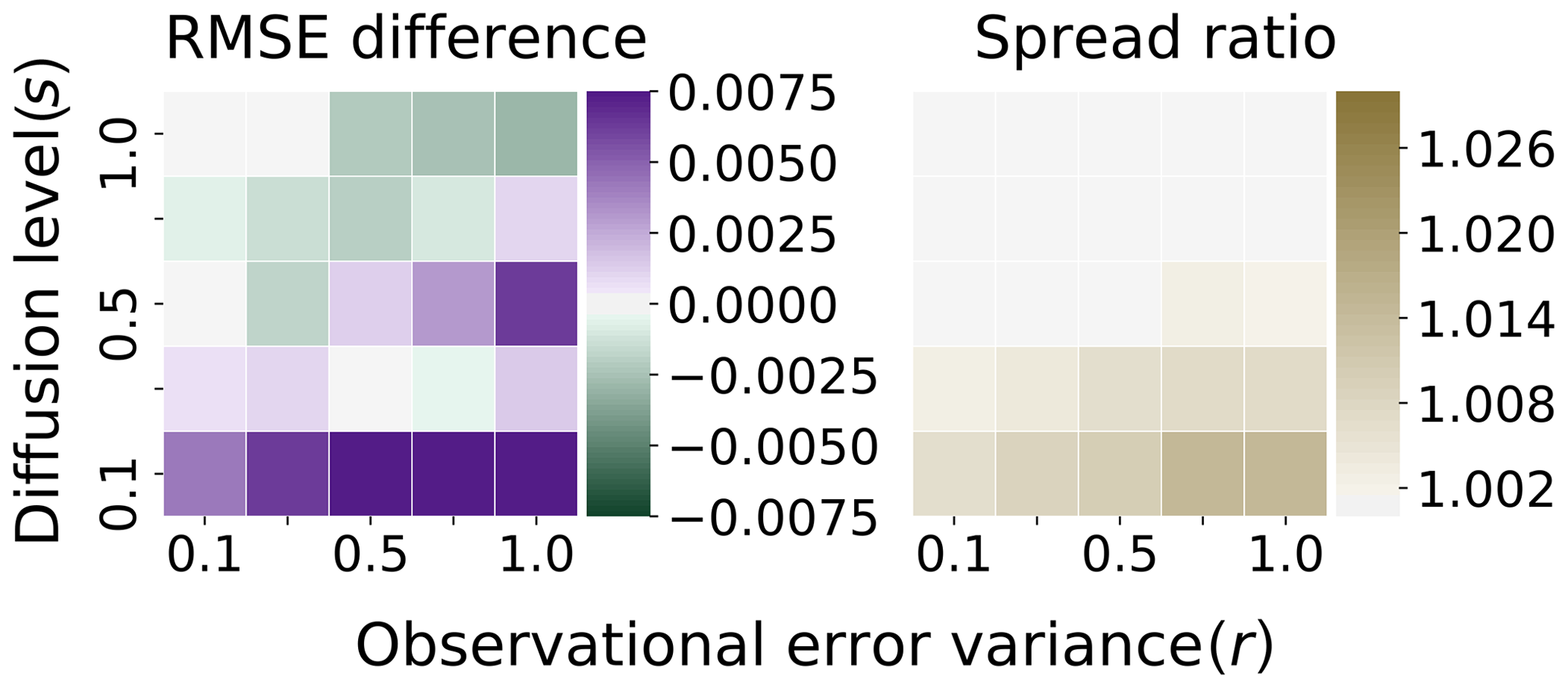
We are secondly interested in seeing how the Euler–Maruyama scheme generating the ensemble compares with the benchmark system when using a maximal time step of . In Fig. 7, the test system uses the Euler–Maruyama scheme with time step . Note, the scale for the RMSE difference in Fig. 7 matches the scale of the positive differences in Fig. 6. However, the scale for the spread ratio in Fig. 7 differs from the scale in Fig. 6 by about an order of magnitude. We find that in contrast to the coarse-grained Runge–Kutta scheme, there is indeed structure in this plot, similar to the results in Sect. 3.2. For low levels of diffusion, there is a clear bias introduced by the Euler–Maruyama scheme in which the ensemble is artificially inflated and also has a lower overall accuracy (though by a small measure). However, it is also of interest that the performance of the Euler–Maruyama scheme and the benchmark system are almost indistinguishable for higher levels of diffusion. With a time step of , the Euler–Maruyama scheme achieves comparable performance with the benchmark approach for high levels of diffusion; however, there is clearly a bias introduced that systematically affects the accuracy of the filter in a low-diffusion regime, in contrast with the last example.
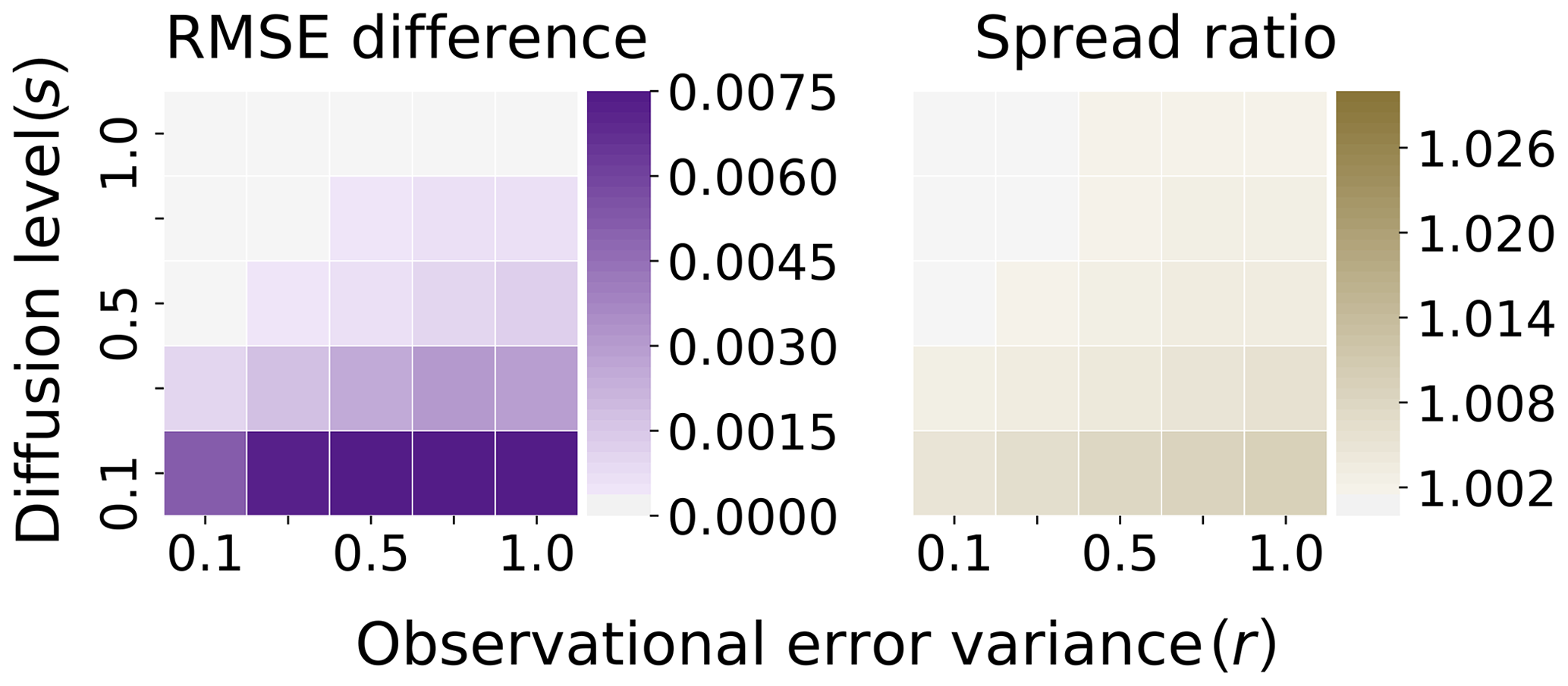
Figure 7Truth: Taylor . Ensemble: Euler–Maruyama . Difference in RMSE/ratio of spread with benchmark Fig. 5.
Next we turn our attention to Fig. 8, where the test system uses the Euler–Maruyama scheme with a time step of . Here, a log scale is introduced in the measure of the RMSE difference, and a new linear scale is introduced for the spread ratio. We see the same structure of the bias introduced to the filter, where for low-diffusion levels there is a strong bias, sufficient to cause filter divergence in this configuration. However, for high-diffusion levels, this bias is less significant, and the filter performance is roughly comparable to the benchmark system, with the difference being of order 10−2 for s≥0.5. We again see the artificial effect of the inflation due to the Euler–Maruyama scheme in the spread of the ensemble, with the same structure present as in the last example. In Fig. 8, the scale for the spread is also about an order of magnitude larger than in Fig. 7.
3.3.2 Varying the truth-twin accuracy for data assimilation
Finally, we examine the effect of lowering the accuracy of the truth twin on the filter performance of the test system relative to the benchmark configuration. In each of the following figures, we again compare the RMSE and spread of the benchmark configuration in Fig. 5 – in all cases the test system will generate the truth twin using the order 2.0 Taylor scheme, with a coarser time step of . In this case, based on the estimate from Table 1, the discretization error for the truth twin is close to 10−3.
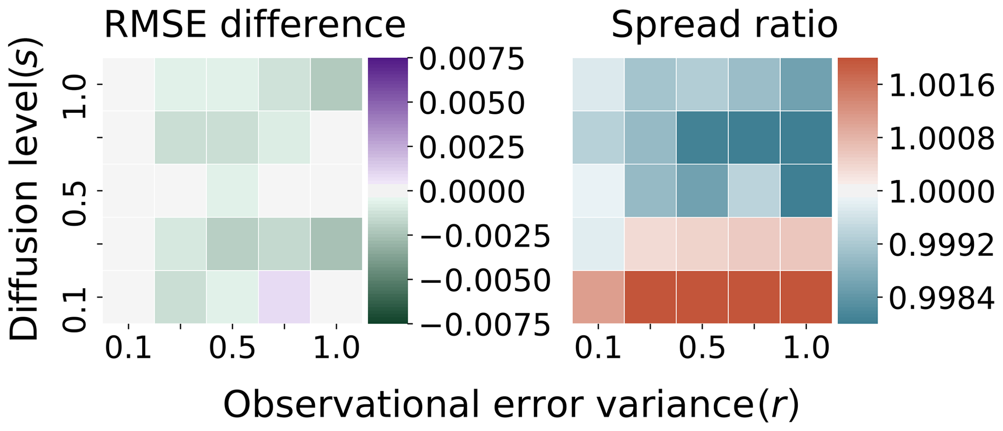
Figure 9Truth: Taylor . Ensemble: Runge–Kutta . Difference in RMSE/ratio of spread with benchmark Fig. 5.
In Fig. 9, the Runge–Kutta scheme generates the ensemble with a step size of . The figure uses identical scales for both RMSE and spread as in Fig. 6. The filtering statistics, with reduced accuracy of the truth twin in conjunction with the reduced accuracy Runge–Kutta scheme for the ensemble, are very similar to the case of the more accurate truth twin. The discretization error in the generation of the ensemble forecast is around in the high-diffusion regime but is usually lower for the smaller diffusion levels (see Table 1).
The main distinction lies in that there is a clear separation of the spread ratio between the low-diffusion and high-diffusion regimes. For this coarse discretization configuration, there is a trend of higher spread in the low-diffusion, versus the trend of lower spread in high-diffusion, as compared with the benchmark system. We test for non-Gaussian structure in the RMSE differences using the Shapiro–Wilk test, with a resulting p value of approximately 0.87. Without significant departures from Gaussianity, we use a t test with the null hypothesis that the RMSE differences are distributed with a mean of zero. The result is a p value of order 𝒪(10−4), indicating that there is significant additional structure in this regime that was not present when the finely discretized truth twin was used. The differences no longer appear to be unbiased, though the differences in this configuration from the benchmark configuration remain practically small for twin experiments; the mean of the RMSE differences in Fig. 9 is approximately , while the standard deviation is approximately . The difference in the spread from 1.0 is approximately on average, with a standard deviation of approximately 10−3.
As a final comparison with the benchmark system, in Fig. 10 the test system generates the ensemble using the Euler–Maruyama scheme with time step . The scale for the RMSE differences is the same as in Fig. 6, while the scale for the ratio of the spread is the same as in Fig. 7. We note that the qualitative structure of the differences is close to that in Fig. 7, with a notable difference. Here, the difference from the benchmark system at high-diffusion levels is relaxed, and the EnKF generated by the fine-grained evolution under Euler–Maruyama at times performs better than the benchmark system, when there is the additional discretization error of the truth twin. This may correspond to the fact that the discretization error for the truth twin under the Taylor scheme is slightly higher with the higher diffusion levels. However, the overall bias introduced by the Euler–Maruyama scheme into the twin experiment seems to remain largely the same. We neglect a plot comparing the system in which the ensemble is generated by the Euler–Maruyama scheme with step – this case is largely the same as results in Fig. 8, with a similar pattern of filter divergence at low diffusion and relaxation at higher diffusion.
3.4 An efficient framework for twin experiments
We briefly consider the computational complexity of the Euler–Maruyama scheme in Eq. (6), the strong order 1.0 stochastic Runge–Kutta scheme in Eq. (8) and the strong order 2.0 Taylor scheme in Eq. (14). We note that every one of these methods applied in the L96-s system has a per-iteration complexity that grows linearly in the system dimension n. This is easy to see for the Euler–Maruyama scheme and is verified by, e.g., Hansen and Penland (2006) for the stochastic Runge–Kutta scheme. On the other hand, it may appear that the numerical complexity of one iteration of the Taylor scheme is 𝒪(n2) due to the multiplication of the vectors f and with the Jacobian ∇f. However, for any n≥4, there are only four nonzero elements in each row of ∇f; the sparsity of the Jacobian means that an efficient implementation of the matrix multiplication will only grow in complexity at 𝒪(n).
However, there are significant differences in the number of iterations necessary to maintain a target discretization error over an interval [0,T]. A typical forecast length T for a twin experiment in the L96-s system is for , corresponding to weakly and strongly nonlinear behavior respectively at the endpoints of this interval. The necessary number of iterations to produce a truth twin with discretization error on 𝒪(10−6) as in the usual Lorenz-96 system is around 𝒪(102) to 𝒪(103) integration steps with the strong order 2.0 Taylor scheme. This is because, even with the order 2.0 strong convergence, the Taylor scheme has to compensate for the large constant term by dropping to a maximal step size of 𝒪(10−4). As a practical compromise, we suggest a higher target discretization error on the order of 𝒪(10−3).
The order 2.0 Taylor scheme, with a maximal step size of , achieves a strong discretization error close to 10−3 across all diffusion regimes. This order of strong discretization error is not possible with either the Euler–Maruyama or Runge–Kutta scheme without dropping the maximal step size to at most 10−3, making the order 2.0 Taylor scheme a suitable choice for generating the truth twin. On the other hand, in ensemble-based DA, the greatest numerical cost in a twin experiment lies in the generation of the ensemble forecast. Across the diffusion regimes, from weak s=0.1 to strong s=1.0, we have seen that the stochastic Runge–Kutta scheme achieves a weak discretization error bounded by 10−3 when the maximal step size is . This suggests the use of a hybrid approach to simulation in which the Taylor and Runge–Kutta schemes are used simultaneously for different scopes.
The combination of (i) truth twin – Taylor with – and (ii) model-twin – Runge–Kutta with – maintains the target discretization error at approximately 10−3 with relatively few computations. Moreover, using the Runge–Kutta scheme to generate the ensemble has the benefit that it is easy to formulate in vectorized code over the ensemble. In Sect. 3.2 and 3.3, we demonstrated that this configuration does not practically bias the ensemble forecast or the DA cycle as compared with more accurate numerical discretizations. While there were small differences noted in some of the short-term forecast statistics, the climatological statistics remain largely the same. Likewise, the differences in the asymptotic filtering statistics appear to be tantamount to numerical noise when compared with a more accurate configuration. Given the results in Sect. 3.2 on the differences for the short-range ensemble forecast statistics with the coarsely resolved Runge–Kutta scheme, we expect the conclusions to hold for standard DA twin experiments with forecasts of length .
In this work, we have examined the efficacy of several commonly used numerical integration schemes for systems of SDEs when applied to a standard benchmark toy model. This toy model, which we denote L96-s, has been contextualized in this study as an ideal representation of a multiscale geophysical model; this represents a system in which the scale separation between the evolution of fast and slow variables is taken to its asymptotic limit. This toy model, which is commonly used in benchmark studies, represents a perfect–random model configuration for twin experiments. In this context, we have examined specifically the following: (i) the modes and respective rates of convergence for each discretization scheme and (ii) the biases introduced into ensemble-based forecasting and DA due to discretization errors. In order to examine the efficacy of higher-order integration methods, we have furthermore provided a novel derivation of the strong order 2.0 Taylor scheme for systems with scalar additive noise.
In the L96-s system, our numerical results have corroborated both the studies of Hatfield et al. (2018) and Frank and Gottwald (2018). We find that the Euler–Maruyama scheme actually introduces a systematic bias in the ensemble forecasting in the L96-s system. However, the effect of this bias on the DA cycle also strongly depends on the observation and, to a larger extent, model uncertainty, represented by amplitude of the random forcing. When the intensity of the model noise, governed by the strength of the diffusion coefficient, is increased, we often see low-precision numerics performing comparably to higher-precision discretizations in the RMSE of filter twin experiments. Indeed, in the high-diffusion regime the state evolution becomes dominated by noise, and the numerical accuracy of the ensemble forecast becomes less influential on the filter RMSE. However, in lower-model-noise regimes and with low-precision numerics, the bias of the Euler–Maruyama scheme is sufficient to produce filter divergence.
Weighing out the overall numerical complexity of each of the methods and their respective accuracies in terms of mode of convergence, it appears that a statistically robust configuration for twin experiments can be achieved by mixing integration methods targeted for strong or weak convergence respectively. Specifically, the strong order 2.0 Taylor scheme provides good performance in terms of strong convergence when the time step is taken . This guarantees a bound on the path-discretization error close to 10−3. On the other hand, the extremely generous coefficient in the bound for weak discretization error for the Runge–Kutta scheme makes this method attractive for ensemble-based forecasting and for deriving sample-based statistics. While the performance depends strongly on the overall level of diffusion, a time step of bounds the weak convergence discretization error by 10−3 for all of the studied diffusion levels.
Generally, it appears preferable to generate the ensemble forecast with the Runge–Kutta scheme and step size . However, we find that the slight increase in error in the ensemble forecast by increasing the step size of the stochastic Runge–Kutta scheme to does not add any systematic bias. This is observed in terms of the short-timescale forecast statistics, the long-timescale climatological statistics and in the filtering benchmarks. In all cases, it appears that additional variability is introduced in the form of noise, yet this appears to be largely unbiased, Gaussian numerical error. In contrast, with the Euler–Maruyama scheme we observe structural bias in the low-diffusion regimes, which is enough to cause filter divergence when the step size is . Especially interesting, this is in the presence of what appears to be an artificial inflation of the ensemble spread with respect to the benchmark system.
Varying the accuracy of the truth-twin simulation, the results are largely the same as in a configuration with a finer step size. Disentangling a direct effect of the discretization error of the truth twin from the effect of, e.g., observation error or the diffusion in the process is difficult. Nonetheless, it appears that higher discretization accuracy of the truth twin places a more stringent benchmark for filters in systems with less overall noise, especially due to the diffusion in the state evolution. There appears to be some relaxing of the RMSE benchmark when diffusion is high and the accuracy of truth twin is low – in these cases we see lower RMSE overall for the coarsely evolved filters than in the benchmark system.
We suggest a consistent and numerically efficient framework for twin experiments in which one produces (i) the truth twin, with the strong order 2.0 Taylor scheme using a time step of , and (ii) the model twin, with the stochastic Runge–Kutta scheme using a time step of . In all diffusion regimes, this guarantees that the discretization error is close to 10−3 and, most importantly, does not introduce a practical bias on the filter results versus the more accurate benchmark system presented in this work. Our results indicate that this configuration is a practical balance between statistical robustness and computational cost. We believe that the results will largely extend to deterministic versions of the EnKF (Carrassi et al., 2018; see Sect. 4.2 and references therein) , though one may encounter differences with respect to tunable parameters, e.g., ensemble sizes, ensemble inflation and/or localization of the scheme.
As possible future work, we have not addressed the efficacy of weak schemes, which are not guaranteed to converge to any path whatsoever. Particularly of interest to the DA community and geophysical communities in general may be the following question: can generating ensemble forecasts with weak schemes reduce the overall cost of the ensemble forecasting step by reducing the accuracy of an individual forecast, while maintaining a better accuracy and consistency of the ensemble-based statistics themselves? Weak schemes often offer many reductions in the numerical complexity due to the reduction of the goal to producing an accurate forecast in distribution alone. Some methods that will be of interest for future study include, e.g., the weak order 3.0 Taylor scheme with additive noise (Kloeden and Platen, 2013; see p. 369) or the weak order 3.0 Runge–Kutta scheme page (Kloeden and Platen, 2013; see p. 488). Additionally, it may be of interest to study other efficient, higher-order strong Runge–Kutta schemes as discussed by Rößler (2010).
A1 The abstract integration rule
We consider the SDE in Eq. (5), in the case where the noise covariance is scalar, though possibly of time-dependent intensity; S will be assumed equal to s(t)In for some scalar function . Suppose the state of the ith component of the model at time tk is given by and . From p. 359 of Kloeden and Platen (2013), the strong order 2.0 Taylor integration rule for xk in Eq. (5) is written component-wise as
where the righthand side of Eq. (A1) is evaluated at (xk,tk) and the terms are defined as follows:
-
Equation (A1a) is the deterministic second-order Taylor method. The differential operator , defined on p. 339 of Kloeden and Platen (2013), in the case of autonomous dynamics, , with additive noise, , reduces to
such that the term .
-
, where Wi(t) is a 1-dimensional Wiener process. By definition, Wi(0)=0 with probability 1, and is a mean zero, Gaussian-distributed random variable with variance equal to Δ.
-
For each l and j, the differential operators and are defined on p. 339 of Kloeden and Platen (2013). In the case of additive noise with scalar covariance, , these operators reduce to
-
For each l and j the terms J(j,0) and , defined on pp. 200–201 of Kloeden and Platen (2013), describe a recursive formulation of multiple Stratonovich integrals of the component random variables of W(t), over an interval of [0,Δ]. These are given as
-
Coefficients Al,j, and bj, in Eqs. (A4a)–(A4e), are defined on pp. 198–199 and 201, via the component-wise Karhunen–Loève Fourier expansion (Kloeden and Platen, 2013; see pp. 70–71) of a Brownian bridge process , for . We write the expansion of B(t) component-wise as
The random Fourier coefficients aj,r and bj,r are defined for each , with
as pairwise-independent, Gaussian-distributed random variables,
The convergence of the righthand side of Eq. (A5) to the left-hand side is in the mean-square sense (L2 norm) and uniform in t. From the Fourier coefficients, for each j, we define aj and bj as
and the auxiliary coefficients as
Expanding Eq. (A1) in the above-defined terms gives an explicit integration rule that has strong convergence of order 2.0 in the maximum step size. The subject of the next section is utilizing the symmetry and the constant/vanishing derivatives of the Lorenz-96 model to derive significant reductions of the above general rule.
A2 Deriving reductions to the rule for L96-s
We note that
from which we derive
The constancy of the second derivatives in Eq. (A14) will allow us to simplify the expressions in Eq. (A1b). Specifically, notice that
such that the sum reduces to
We are thus interested in reducing the terms of Eq. (A16) via antisymmetry within with respect to the arguments l and j. We note that
and combining these relationships with the definition in Eq. (A4b), we find
Notice that from Eqs. (A4c) and (A4d), the sum contains the terms on the left-hand side of Eq. (A20),
Combining terms as in the left-hand side of Eq. (A20) and substituting the righthand side of the terms in Eq. (A20) we derive that
Note then, from Eq. (A19), that we need to combine the terms of the symmetric sum in l and j,
We thus use the antisymmetry in the terms in Eq. (A21) to make further reductions. Note that from Eq. (A4e) we have
Therefore, the symmetric sum in l and j of is given by
Thus using Eq. (A24), the symmetric sum of Eq. (A21b) in l and j equals
Likewise, taking the sum of Eq. (A21c) symmetrically in l and j equals
Recalling the antisymmetry of Al,j and the substitutions in Eqs. (A25) and (A26), we combine the terms to derive
Finally, using Eq. (A27), let us define the symmetric function in (l,j),
from the above definition and Eq. (A16), we recover the expression
Furthermore, define the random vectors
Using the above definitions, we can write the integration rule in a matrix form as
Once again, Eq. (A31a) is the standard deterministic order 2.0 Taylor rule but written in matrix form. On the other hand, the additional term in Eq. (A31b) resolves at second-order the SDE form of L96 with additive noise of scalar covariance (L96-s).
A3 Finite approximation and numerical computation
So far we have only presented an abstract integration rule that implicitly depends on infinite series of random variables. Truncating the Fourier series for the components of the Brownian bridge in Eq. (A5), we define a random process
from which we will define a numerical integration rule, depending on the order truncation p. Key to the computation of the rule is that, by way of the approximations on pp. 202–204 of Kloeden and Platen (2013), it is representable as a function of mutually independent, standard Gaussian random variables. We will denote these standard Gaussian random variables as and ϕj,p, and for each , and all , we define
where
It is important to note that, while are defined as an infinite linear combination of the random Fourier coefficients, we take μj,p and ϕj,p as drawn iid from the standard Gaussian distribution and use their functional relationship to the Fourier coefficients to approximate the Stratonovich integral. The coefficients ρp and αp normalize the variance in the remainder term in the truncation of the Brownian bridge process to the finite sum . Using the above-defined random variables in Eq. (A33) and auxiliary deterministic variables in Eq. (A34), we will define the pth approximation of the multiple Stratonovich integrals in Eqs. (A4e)–(A4c).
For any and for each , we can recover the term bj directly from the functional relationships in Eq. (A33), and we recover aj by the relationship on p. 203 of Kloeden and Platen (2013),
The auxiliary function Cl,j is truncated at the pth order, defined on p. 203 of Kloeden and Platen (2013), as
While the choice of p modulates the order of approximation of the Stratonovich integrals, it is important to note that in our case the choice of p>1 is unnecessary. Actually, all terms in the Stratonovich integrals in the integration rule we have derived are exact except for the terms of . Up to a particular realization of the random variables, aj and bj are constructed identically from the full Fourier series. It is thus only the terms of that are truncated, and this approximation appears at order 2.0 in the integration step. Therefore, up to a constant that depends on p, the approximation error of the Stratonovich integrals is also at order 2.0. Note that, by definition, when p=1, for all . Therefore, we may eliminate this term in our finite approximation without loss of the order of convergence.
For simplicity, at each integration step for each , , we may draw iid standard Gaussian random variables, and ϕj,p, to obtain an approximation of the recursive Stratonovich integrals in Eq. (4). For each j we will make substitutions as described in Eqs. (A34)–(A35) to obtain the final integration rule. Using the simplifications made to the rule in Sects. A and A2 and the above discussion, we define
Finally, we define the following random vectors
such that we obtain the integration rule in matrix form,
The constants ρp and αp can be computed once for all steps, with truncation taken at p=1 such that
Then, for each step of size Δ, we can follow the rule outlined in Eq. (14).
When we benchmark the convergence of the strong order 2.0 Taylor scheme to a finely discretized reference path xSP, the formulation for generating the Taylor scheme discretized solution differs from the direct implementation in Sect. 2.5. The strong order 2.0 Taylor scheme approximately resolves the multiple Stratonovich integrals, Eq. (A4), using combinations of the Karhunen–Loève Fourier coefficients for the Brownian bridge process, Eq. (A5), between the discretization points. The realization of the Brownian motion at the discretization times is independent of the realizations of the Brownian bridge in between these times such that, when simulating an arbitrary sample path with the Taylor scheme, one can simply use the functional relationships described in Sect. 2.5 to define the linear combinations in Eq. (A33). Therefore, if there is no concern about discretizing a specific reference path then drawing iid realizations for the standard normal variables and ϕj,p is sufficient.
With regard to a specific reference path xSP discretized with time step ΔSP smaller than the Taylor scheme step of Δq, we must use the known realizations of the Brownian motion at steps ΔSP in between the coarse steps Δq to compute the Brownian bridge. The random vector b is defined functionally in Eq. (A9) as an infinite sum of vectors of random Fourier coefficients such that there is an additional dependence on the order of truncation p of the term b in our benchmarks. This again differs substantially from the case in which we wish to simulate some arbitrary path with the Taylor scheme; in this case, the relationship between b and the Fourier coefficients is defined by an analytical, functional relationship, and it is sufficient to make a truncation order p=1 to other terms to maintain order 2.0 strong convergence.
As a modification of the Taylor scheme, utilizing the known realization of the Brownian bridge process between the discretization steps Δq, we compute the Fourier coefficients of the Brownian bridge, up to pth order, directly by the right-Riemann sums approximating Eqs. (A6)–(A7), with discretization step size ΔSP. With respect to all of our benchmarks, we found no significant difference in performance when directly computing only the order p=1 and the order p=25 Fourier coefficients as described above, so we present only the p=1 case for simplicity.
The current version of model is available from the project website via https://doi.org/10.5281/zenodo.3366374 under the MIT License. The exact version of the model used to produce the results used in this paper is archived on Zenodo (Grudzien, 2020), as are scripts to run the model and produce the plots for all the simulations presented in this paper (Grudzien, 2020).
CG derived the order 2.0 Taylor discretization for the L96-s model, developed all model code and processed all data. CG and MB reviewed and refined mathematical results together. All authors contributed to the design of numerical experiments. CG wrote the paper with contributions from MB and AC.
The authors declare that they have no conflict of interest.
This work benefited from funding by the project REDDA of the Norwegian Research Council. Alberto Carrassi was also supported by the Natural Environment Research Council. This work benefited significantly from CEREA hosting Colin Grudzien as a visiting researcher in 2018, during his postdoctoral appointment at NERSC. CEREA is a member of the Institut Pierre-Simon Laplace (IPSL). The authors would like to thank Peter Kloeden, Eckhard Platen, Paul Hurtado and the two anonymous referees for their correspondence and suggestions on this work.
This research has been supported by the Norwegian Research Council (grant no. 250711). Alberto Carrassi was also supported by the Natural Environment Research Council (agreement PR140015 between NERC and the National Centre for Earth Observation).
This paper was edited by James R. Maddison and reviewed by two anonymous referees.
Arnold, H. M., Moroz, I. M., and Palmer, T. N.: Stochastic parametrizations and model uncertainty in the Lorenz'96 system, Phil. Trans. R. Soc. A, 371, 20110479, https://doi.org/10.1098/rsta.2011.0479, 2013. a
Berry, T. and Harlim, J.: Linear theory for filtering nonlinear multiscale systems with model error, Proc. R. Soc. A, 470, 20140168, https://doi.org/10.1098/rspa.2014.0168, 2014. a
Bocquet, M. and Carrassi, A.: Four-dimensional ensemble variational data assimilation and the unstable subspace, Tellus A, 69, 1304504, https://doi.org/10.1080/16000870.2017.1304504, 2017. a
Bocquet, M., Gurumoorthy, K. S., Apte, A., Carrassi, A., Grudzien, C., and Jones, C. K. R. T.: Degenerate Kalman Filter Error Covariances and Their Convergence onto the Unstable Subspace, SIAM/ASA J. Uncertainty Quantification, 5, 304–333, 2017. a
Boers, N., Chekroun, M. D., Liu, H., Kondrashov, D., Rousseau, D.-D., Svensson, A., Bigler, M., and Ghil, M.: Inverse stochastic–dynamic models for high-resolution Greenland ice core records, Earth Syst. Dynam., 8, 1171–1190, https://doi.org/10.5194/esd-8-1171-2017, 2017. a
Burrage, K. and Burrage, P. M.: High strong order explicit Runge-Kutta methods for stochastic ordinary differential equations, Appl. Numer. Math., 22, 81–101, 1996. a
Burrage, K. and Burrage, P. M.: General order conditions for stochastic Runge-Kutta methods for both commuting and non-commuting stochastic ordinary differential equation systems, Appl. Numer. Math., 28, 161–177, 1998. a
Carrassi, A. and Vannitsem, S.: Deterministic treatment of model error in geophysical data assimilation, in: Mathematical paradigms of climate science, Springer, 175–213, 2016. a
Carrassi, A., Bocquet, M., Bertino, L., and Evensen, G.: Data Assimilation in the Geosciences-An overview on methods, issues and perspectives, WIREs Clim. Change, 9, e535, https://doi.org/10.1002/wcc.535, 2018. a, b, c, d
Chekroun, M. D., Simonnet, E., and Ghil, M.: Stochastic climate dynamics: Random attractors and time-dependent invariant measures, Physica D, 240, 1685–1700, 2011. a
Chorin, A. J. and Lu, F.: Discrete approach to stochastic parametrization and dimension reduction in nonlinear dynamics, P. Natl. Acad. Sci. USA, 112, 9804–9809, 2015. a, b
Cotter, C., Crisan, D., Holm, D. D., Pan, W., and Shevchenko, I.: Numerically Modeling Stochastic Lie Transport in Fluid Dynamics, Multiscale Model. Sim., 17, 192–232, 2019. a
Crommelin, D. and Vanden-Eijnden, E.: Subgrid-scale parameterization with conditional Markov chains, J. Atmos. Sci., 65, 2661–2675, 2008. a
Demaeyer, J. and Vannitsem, S.: Stochastic Parameterization of Subgrid-Scale Processes: A Review of Recent Physically Based Approaches, in: Advances in Nonlinear Geosciences, Springer, 55–85, 2018. a
Dijkstra, H. A.: Nonlinear climate dynamics, Cambridge University Press, 2013. a
Evensen, G.: The ensemble Kalman filter: Theoretical formulation and practical implementation, Ocean Dynam., 53, 343–367, 2003. a
Frank, J. and Gottwald, G. A.: A Note on Statistical Consistency of Numerical Integrators for Multiscale Dynamics, Multiscale Model. Sim., 16, 1017–1033, 2018. a, b
Frank, J. and Zhuk, S.: A detectability criterion and data assimilation for nonlinear differential equations, Nonlinearity, 31, 5235, https://doi.org/10.1088/1361-6544/aaddcb, 2018. a
Franzke, C., O'Kane, T., Berner, J., Williams, P., and Lucarini, V.: Stochastic climate theory and modeling, WIRES Clim. Change, 6, 63–78, 2015. a
Ghil, M.: The wind-driven ocean circulation: Applying dynamical systems theory to a climate problem, Discrete Cont. Dyn.-A, 37, 189–228, 2017. a
Ghil, M.: A century of nonlinearity in the geosciences, Earth and Space Science, 6, 1007–1042, https://doi.org/10.1029/2019EA000599, 2018. a
Ghil, M., Chekroun, M. D., and Simonnet, E.: Climate dynamics and fluid mechanics: Natural variability and related uncertainties, Physica D, 237, 2111–2126, 2008. a
Gottwald, G. A. and Harlim, J.: The role of additive and multiplicative noise in filtering complex dynamical systems, Proc. R. Soc. A, 469, 20130096, https://doi.org/10.1098/rspa.2013.0096, 2013. a
Gottwald, G. A., Crommelin, D., and Franzke, C.: Stochastic climate theory, Nonlinear and Stochastic Climate Dynamics, 209–240, https://doi.org/10.1017/9781316339251, 2015. a
Gottwald, G. A., Peters, K., and Davies, L.: A data-driven method for the stochastic parametrisation of subgrid-scale tropical convective area fraction, Q. J. Roy. Meteor. Soc., 142, 349–359, 2016. a
Grudzien, C.: cgrudz/lorenz_96_sde: Revision Release, https://doi.org/10.5281/zenodo.3701601, 2020. a, b
Grudzien, C., Carrassi, A., and Bocquet, M.: Asymptotic forecast uncertainty and the unstable subspace in the presence of additive model error, SIAM/ASA J. Uncertainty Quantification, 6, 1335–1363, 2018a. a
Grudzien, C., Carrassi, A., and Bocquet, M.: Chaotic dynamics and the role of covariance inflation for reduced rank Kalman filters with model error, Nonlin. Processes Geophys., 25, 633–648, https://doi.org/10.5194/npg-25-633-2018, 2018b. a
Gurumoorthy, K. S., Grudzien, C., Apte, A., Carrassi, A., and Jones, C. K. R. T.: Rank deficiency of Kalman error covariance matrices in linear time-varying system with deterministic evolution, SIAM J. Control Optim., 55, 741–759, 2017. a
Hansen, J. A. and Penland, C.: Efficient approximate techniques for integrating stochastic differential equations, Mon. Weather Rev., 134, 3006–3014, 2006. a, b, c
Hatfield, S., Düben, P., Chantry, M., Kondo, K., Miyoshi, T., and Palmer, T. N.: Choosing the optimal numerical precision for data assimilation in the presence of model error, J. Adv. Model. Earth Syst., 10, 2177–2191, 2018. a, b
Herrera, S., Pazó, D., Fernández, J., and Rodríguez, M. A.: The role of large-scale spatial patterns in the chaotic amplification of perturbations in a Lorenz'96 model, Tellus A, 63, 978–990, 2011. a
Iacus, S. M.: Simulation and inference for stochastic differential equations: with R examples, Springer Science & Business Media, 2009. a
Jazwinski, A. H.: Stochastic Processes and Filtering Theory, Academic Press, New-York, 1970. a
Kang, E. L. and Harlim, J.: Filtering Partially Observed Multiscale Systems with Heterogeneous Multiscale Methods–Based Reduced Climate Models, Mon. Weather Rev., 140, 860–873, 2012. a
Kloeden, P. and Platen, E.: Numerical Solution of Stochastic Differential Equations, Stochastic Modelling and Applied Probability, Springer Berlin Heidelberg, 2013. a, b, c, d, e, f, g, h, i, j, k, l, m, n, o, p, q, r
Leutbecher, M. and Palmer, T. N.: Ensemble forecasting, J. Comput. Phys., 227, 3515–3539, 2008. a
Lewis, J. M.: Roots of ensemble forecasting, Mon. Weather Rev., 133, 1865–1885, 2005. a
Lorenz, E. N.: Deterministic nonperiodic flow, J. Atmos. Sci., 20, 130–141, 1963. a
Lorenz, E. N.: Predictability: a problem partly solved, in: Predictability, edited by: Palmer, T., European Centre for Medium-Range Weather Forecast, Shinfield Park, Reading, UK, 1996. a, b
Lorenz, E. N.: Designing chaotic models, J. Atmos. Sci., 62, 1574–1587, 2005. a
Lorenz, E. N. and Emanuel, K. A.: Optimal sites for supplementary weather observations: Simulation with a small model, J. Atmos. Sci., 55, 399–414, 1998. a
Lu, F., Tu, X., and Chorin, A. J.: Accounting for Model Error from Unresolved Scales in Ensemble Kalman Filters by Stochastic Parameterization, Mon. Weather Rev., 145, 3709–3723, 2017. a
Maclean, J. and Van Vleck, E. S.: Projected Data Assimilation, arXiv preprint, arXiv:1902.04212, 2019. a
Mitchell, L. and Gottwald, G. A.: Data assimilation in slow–fast systems using homogenized climate models, J. Atmos. Sci., 69, 1359–1377, 2012. a
Palmer, T. N., Shutts, G. J., Hagedorn, R., Doblas-Reyes, F. J., Jung, T., and Leutbecher, M.: Representing model uncertainty in weather and climate prediction, Annu. Rev. Earth Planet. Sci., 33, 163–193, 2005. a
Pichler, L., Masud, A., and Bergman, L. A.: Numerical solution of the Fokker–Planck equation by finite difference and finite element methods–a comparative study, in: Computational Methods in Stochastic Dynamics, Springer, 69–85, 2013. a
Pulido, M., Tandeo, P., Bocquet, M., Carrassi, A., and Lucini, M.: Stochastic parameterization identification using ensemble Kalman filtering combined with maximum likelihood methods, Tellus A, 70, 1442099, https://doi.org/10.1080/16000870.2018.1442099, 2018. a
Raanes, P. N., Carrassi, A., and Bertino, L.: Extending the square root method to account for additive forecast noise in ensemble methods, Mon. Weather Rev., 143, 3857–3873, 2015. a
Raanes, P. N., Bocquet, M., and Carrassi, A.: Adaptive covariance inflation in the ensemble Kalman filter by Gaussian scale mixtures, Q. J. Roy. Meteor. Soc., 145, 53–75, 2018. a
Rößler, A.: Runge–Kutta methods for the strong approximation of solutions of stochastic differential equations, SIAM J. Num. Anal., 48, 922–952, 2010. a
Rüemelin, W.: Numerical treatment of stochastic differential equations, SIAM J. Num. Anal., 19, 604–613, 1982. a
Shapiro, S. and Wilk, M.: An analysis of variance test for normality (complete samples), Biometrika, 52, 591–611, 1965. a
Tranninger, M., Seeber, R., Zhuk, S., Steinberger, M., and Horn, M.: Detectability Analysis and Observer Design for Linear Time Varying Systems, IEEE Contr. Syst. Lett., 4, 331–336, 2019. a
Vissio, G. and Lucarini, V.: A proof of concept for scale-adaptive parametrizations: the case of the Lorenz'96 model, Q. J. Roy. Meteor. Soc., 144, 63–75, 2018. a, b
Whitaker, J. S. and Loughe, A. F.: The relationship between ensemble spread and ensemble mean skill, Mon. Weather Rev., 126, 3292–3302, 1998. a, b
Wilks, D. S.: Effects of stochastic parametrizations in the Lorenz'96 system, Q. J. Roy. Meteor. Soc., 131, 389–407, 2005. a, b
- Abstract
- Introduction
- Numerical simulation of stochastic dynamics for twin experiments
- Numerical benchmarks
- Conclusions
- Appendix A: Deriving the strong order 2.0 Taylor rule for L96-s
- Appendix B: Resolving the strong order 2.0 Taylor scheme for consistent numerical benchmarks
- Code availability
- Author contributions
- Competing interests
- Acknowledgements
- Financial support
- Review statement
- References