Verification of the regional atmospheric model CCLM v5.0 with conventional data and lidar measurements in Antarctica

The nonhydrostatic regional climate model CCLM was used for a long-term hindcast run (2002–2016) for the Weddell Sea region with resolutions of 15 and 5 km and two different turbulence parametrizations. CCLM was nested in ERA-Interim data and used in forecast mode (suite of consecutive 30 h long simulations with 6 h spin-up). We prescribed the sea ice concentration from satellite data and used a thermodynamic sea ice model. The performance of the model was evaluated in terms of temperature and wind using data from Antarctic stations, automatic weather stations (AWSs), an operational forecast model and reanalyses data, and lidar wind profiles. For the reference run we found a warm bias for the near-surface temperature over the Antarctic Plateau. This bias was removed in the second run by adjusting the turbulence parametrization, which results in a more realistic representation of the surface inversion over the plateau but resulted in a negative bias for some coastal regions. A comparison with measurements over the sea ice of the Weddell Sea by three AWS buoys for 1 year showed small biases for temperature around ±1 K and for wind speed of 1 m s⁻¹. Comparisons of radio soundings showed a model bias around 0 and a RMSE of 1–2 K for temperature and 3–4 m s⁻¹ for wind speed. The comparison of CCLM simulations at resolutions down to 1 km with wind data from Doppler lidar measurements during December 2015 and January 2016 yielded almost no bias in wind speed and a RMSE of ca. 2 m s⁻¹. Overall CCLM shows a good representation of temperature and wind for the Weddell Sea region. Based on these encouraging results, CCLM at high resolution will be used for the investigation of the regional climate in the Antarctic and atmosphere–ice–ocean interactions processes in a forthcoming study.

1 Introduction

Regional climate models (RCMs) are a valuable tool for improving our understanding of processes and interactions of the climate system in the polar regions. These processes are, e.g. atmosphere–ice–ocean (AIO) interactions, which are particularly pronounced when sea ice formation is involved. This is associated with strong impacts on the surface energy fluxes and the atmospheric boundary layer (ABL). The added value of RCMs compared to coarser reanalysis and global climate models (GCMs) has been shown in a number of studies (e.g. Rummukainen, 2010) and is the background of the Polar-CORDEX (COordinated Regional Downscaling Experiment) initiative (Akperov et al., 2018). For the polar regions, the spatial and temporal coverage by the observational network is sparse compared to midlatitudes; therefore RCMs are the only means of providing climatological information at a high resolution with full spatial coverage (e.g. Kohnemann et al., 2017). High-resolution atmospheric simulations are also important for forcing ocean models (Haid et al., 2015) and the understanding of the surface mass balance (Souverijns et al., 2018; Gorodetskaya et al., 2014). A high resolution is also necessary to resolve topographic effects such as foehn winds, which could play a role for the instability of ice shelves (Cape et al., 2015), and katabatic winds (Ebner et al., 2014; Heinemann, 1997).

For the Antarctic, van Lipzig (2004) showed that for a sufficient consideration of topography-induced atmospheric processes a resolution of at least 15 km is necessary. The hydrostatic regional climate model RACMO (Regional Atmospheric Climate Model) was used by van Lipzig (2004) with a 14 km resolution for the period 1987–1993. The RACMO model was also used by van Wessem et al. (2015) at a high resolution of 5.5 km over the period 1979–2013 for the Antarctic Peninsula (AP), and more detailed and more pronounced temperature and wind speed gradients compared to the ERA-Interim forcing (approx. 80 km horizontal resolution) were found, which are mostly related to the katabatic wind. However, the sea ice cover data set with 80 km resolution and the assumption that nonhydrostatic effects are small at 5 km resolution are drawbacks of that study. Foehn winds were studied by Elvidge et al. (2015) particularly for the Larsen C ice shelf using the Met Office Unified Model at 1.5 km grid size. King et al. (2017) used model data from the Antarctic Mesoscale Prediction System (AMPS) with 5 km resolution for the summer season 2010/11 to also study foehn wind effects over the Larsen C Ice Shelf. Turton et al. (2017) studied foehn effects over the Larsen C Ice Shelf in May 2011 using the nonhydrostatic polar WRF model with 1.5 and 5 km resolution and found in general better results for the higher resolution. These studies were performed with nonhydrostatic models but for rather short periods. The need for nonhydrostatic models for high-resolution regional climate simulations is outlined by Giorgi and Gutowski (2015) and Prein et al. (2015).

In the present study the regional nonhydrostatic Consortium for Small-Scale Modeling (COSMO) model in Climate Mode (COSMO-CLM; abbreviated as CCLM) is used to run simulations for the Antarctic with resolutions of ≈15 and ≈5 km for the time period from 2002 to 2016. The simulation is forced with ERA-Interim reanalysis data and is the first long-term hindcast simulation with a high-resolution nonhydrostatic regional climate model for the Weddell Sea region. The main purpose of the simulations is the study of AIO interactions in polynyas (see Ebner et al., 2014), which require a high resolution also in the sea ice data used as boundary conditions for the simulations. Thus we focus on the period since 2002, for which high-resolution sea ice data from microwave satellite sensors are available (see Sect. 2). The CCLM data are also used as atmospheric forcing for a high-resolution sea ice/ocean model (see Haid et al., 2015).

This data set of atmospheric variables is compared to conventional measurements like radio soundings (RSs) and both manned stations (MSs) and automatic weather stations (AWSs). Further, an investigation is presented concerning the usage of Doppler wind lidar measurements in polar regions for verifications of model simulations. In Sect. 2 the model and data sets used for the simulation and the verification are described, followed by a short comparison to another model and reanalyses (Sect. 3), then the results of the verification (Sect. 4), and finally the summary (Sect. 5) and conclusions (Sect. 6).

2 Data and methods

2.1 CCLM

The CCLM is a regional nonhydrostatic model and is used as the community model for German climate research. It is a modified version of the COSMO model (version 5.0; Steppeler et al., 2003; http://www.cosmo-model.org, last access: 31 March 2020; archived documentation at zenodo; Zentek, 2019) used by the Climate Limited-area Modelling (CLM)-Community (Rockel et al., 2008; http://www.clm-community.eu, last access: 31 March 2020). Three different model setups are used for the simulations (see Table 1 and Fig. 1).

Table 1 Overview of the different simulations. The grid size for C01 and T01 was changed for each day with a minimal (maximal) size of 200×200 (353×464).

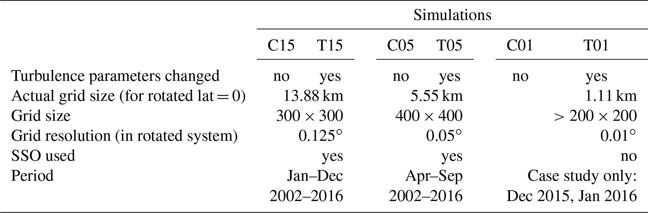
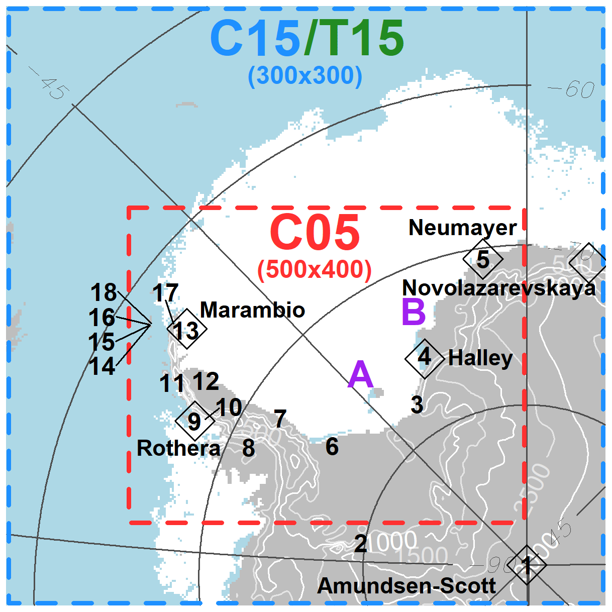
Figure 1 Overview of the C15/T15 (blue/green) and C05 (red) simulation domains, locations of six radio sounding stations (diamonds), surface/automatic weather stations (numbers), and locations of the RV Polarstern during our two case studies A and B (purple). Topography contours are plotted every 500 m, and sea ice concentration >70 % for the 1 June 2015 is shown in white. (Note that the T15 domain is the same as the C15 domain.)

The first simulation with a resolution of ≈15 km (C15) is forced with ERA-Interim (Dee et al., 2011) for the time period from 2002 to 2016, and the domain covers a quarter of Antarctica centred over the Weddell Sea. The second simulation with a resolution of ≈5 km (C05) is nested inside the C15 domain and is only done for winter periods (April–September) in 2002–2016. The third simulation (T15) uses the same setup as C15, but the turbulence parametrization was changed, since deficits in the C15 simulations were found for the stable boundary layer. These modifications are based on the studies of Cerenzia et al. (2014), Hebbinghaus and Heinemann (2006), and Souverijns et al. (2019). In the standard version of CCLM, the diffusion coefficients for heat and momentum are restricted to the minimal value of 0.4 m² s⁻¹. In the T15 simulation, these minimal diffusion coefficients were set to 0.01 m² s⁻¹ to allow for a very stable boundary layer (SBL) over the Antarctic ice sheet during winter. Further, the standard setup of CCLM uses a parametrization of the impact of the inhomogeneity of the surface via the energy transfer from subgrid-scale eddies on the turbulent kinetic energy (TKE). Since this leads to an overestimation of the TKE in the SBL (Cerenzia et al., 2014), this parametrization was removed in the T15 runs.

All simulations have a vertical resolution of 60 levels that are terrain-following on the ground and gradually change into pressure-following coordinates around a height of 12 km with the model top being at 25 km. The runs were performed in a forecast mode, i.e. daily 30 h simulations to keep the hindcast close to reality. We used the first 6 h as spin-up in order to allow for the atmosphere to adapt to the difference between the high-resolution sea ice data from satellite and the coarse-resolution temperatures from ERA-Interim.

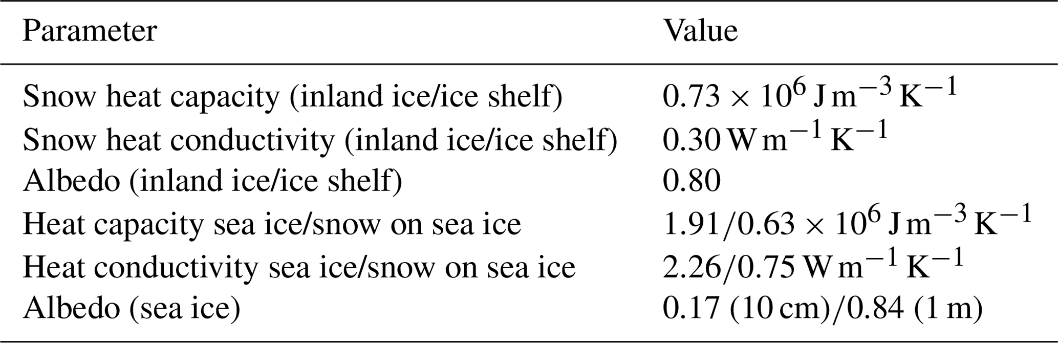
Over land, we use the standard land surface model of CCLM (TERRA; see archived documentation at zenodo; Zentek, 2019). The soil model has eight layers (down to 15 m) and allows for an additional snow layer on top of the soil, which varies with precipitation and sublimation. For the land ice regions, soil was replaced by snow using the parameters listed in Table 2. Over sea ice the model was adapted to polar regions by the implementation of a thermodynamic sea ice model (Schröder et al., 2011). The snow temperature profile is initialized with the forcing data, and then the snow temperatures freely evolve. The surface albedo for inland ice and ice shelves is kept constant and has no seasonal variations. The albedo of sea ice is parametrized as a function of ice thickness and temperature by a modified Køltzow scheme (Køltzow, 2007) as described in Gutjahr et al. (2016).

Table 2 Overview of surface parameters.

Further, the RTopo2 data set (Schaffer and Timmermann, 2016; Schaffer et al., 2016) is used for the topography as the default data set of CCLM did not include ice shelves. Parameters for the subgrid-scale orography (SSO; Lott and Miller, 1997) module were computed for the new data set, and the SSO module was used for both the 15 and 5 km simulation.

For sea ice data, daily sea ice concentration (SIC) is used. The data are based on AMSR-E (Advanced Microwave Scanning Radiometer – for Earth Observing System) and AMSR2 (Advanced Microwave Scanning Radiometer 2), and for data gaps SSMIS (Special Sensor Microwave Imager/Sounder) satellite measurements (Spreen et al., 2008; Ezraty et al., 2007) are used. The resolution of the sea ice concentration data is 6.25 km for AMSR-E/AMSR2 but is coarser for SSMIS (12.5 km). Details of the data used are given in Table 3. Sea surface temperature (SST) data and initial surface temperature were taken from ERA-Interim. In the case of inconsistency between SST and SIC (surface temperature below the freezing temperature of −1.7 ^∘C for a SIC of 0 %), the SST was set to the freezing temperature. The SIC data included some missing values, which were replaced in the following way. In a first step, missing values were filled with values from the day before and after (mean if both were available). In a second step, days for which no data were available were interpolated linearly in time (overall 35 d; maximal 9 d in succession). This still left some missing values (mostly along the coastline due to the different land masks of RTopo2 and AMSR-E/SSMIS/AMSR2). These remaining missing values are filled in a third step with an iterative procedure for each day separately using the surrounding grid points.

Table 3 Overview of sea ice concentration data used in CCLM. Download for CERSAT/IFREMER athttp://cersat.ifremer.fr/data/ (last access: 31 March 2020) and for Uni Bremen at https://seaice.uni-bremen.de/start/data-archive/ (last access: 31 March 2020).

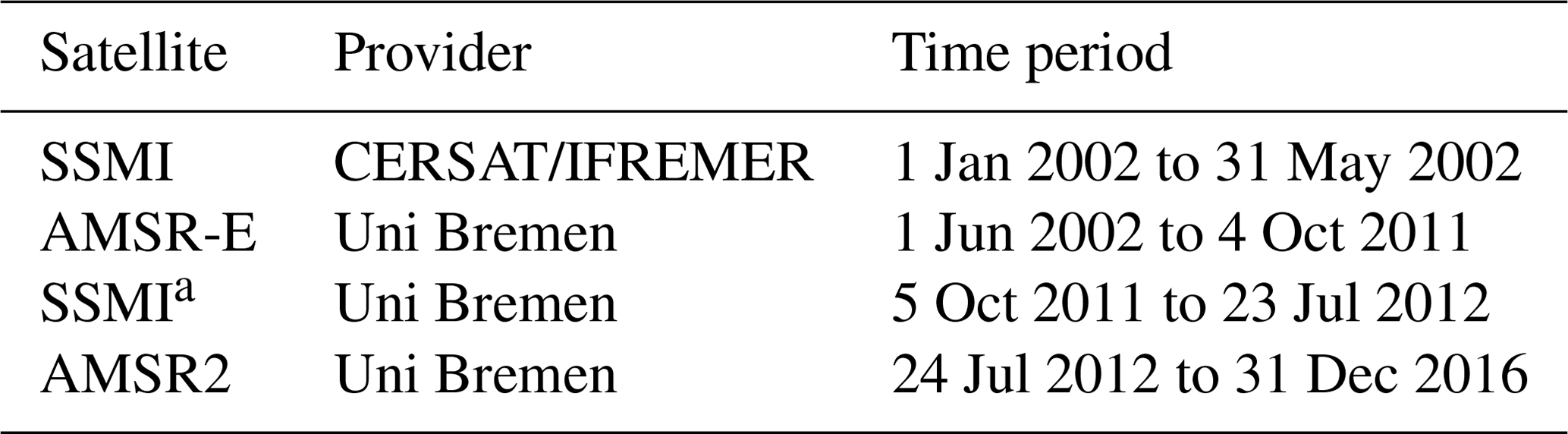
^a There were two data sets of SSMI data based on different sensors (F17 and F18). A comparison for the overlapping periods of 2 months (August, September) with AMSR-E (2011) and AMSR2 (2012) were compared with the F17 and F18 SSMI
data. Standard deviation was computed, and it was found that F17 is closer to
AMSR-E and F18 is closer to AMSR2, but overall F17 seemed to have less
deviation in the area of interest. So only the F17 data were taken for October
2011–July 2012.

A fractional sea ice cover is not used in the model, thus for each grid box there is only one value of sea ice thickness, which is assumed to cover the whole grid box. Benefits of modelling a fractional sea ice cover are investigated in Gutjahr et al. (2016). As daily sea ice thickness data like PIOMAS (Zhang and Rothrock, 2003) are not available for Antarctica, we assume two different ice classes depending on the initial sea ice concentration. Grid points with a sea ice concentration of 0 %–15 % are set to open water. For 15 %–70 % a sea ice thickness of 0.1 m is assumed (see e.g. Gutjahr et al., 2016). For 70 %–100 % we assume a thickness of 1 m, which is a reasonable estimate for the Weddell Sea (see Kurtz and Markus, 2012). With a threshold of 70 % SIC commonly used for the identification of polynyas, this choice is in accordance with previous studies (Ebner et al., 2014; Bauer et al., 2013). For grid points with a sea ice thickness of 0.1 m the modified Køltzow scheme yields an albedo of 0.07, and we assume no snow cover. For a thickness of 1 m the albedo is 0.84 (for temperatures lower than −2 ^∘C) and a fixed snow layer of 10 cm snow cover (Schröder et al., 2011) is assumed.

Lastly we want to point out some differences between the present model setup and the setup of Souverijns et al. (2019), as they also used the CCLM model for simulations in the Antarctic. Souverijns et al. (2019) used CCLM with the community land model CLM (van Kampenhout et al., 2017), while we used default land surface model of CCLM with the adaptions described above. While we used daily high-resolution (6 km) sea ice data from satellites, they used coarse-resolution ERA-Interim data (80 km) for the sea ice. In addition, they used only the standard one-layer sea ice model of CCLM. They also ran CCLM in climate mode and applied spectral nudging, while we used forecast mode with a restart every day and applied forcing only at the boundaries.

2.2 AMPS and ERA

Beside the forcing data set ERA-Interim (Dee et al., 2011), the newer ERA5 reanalysis data (Hersbach et al., 2018) and data from the Antarctic Mesoscale Prediction System (AMPS; Bromwich et al., 2005; Powers et al., 2012) are used for comparisons. ERA5 reanalysis data are the new version of ERA-Interim reanalysis data. Both data sets are products of the European Centre for Medium-Range Weather Forecasts. The AMPS data set was produced as a collaborative effort between the Mesoscale and Microscale Meteorology Laboratory of the National Center for Atmospheric Research and The Ohio State University. The horizontal/temporal resolutions are approximately 80 km (6 h)⁻¹ (ERA-Interim), 30 km h⁻¹ (ERA5), and 10 km (3 h)⁻¹ (AMPS).

2.3 AWSs and surface stations

We use near-surface temperature and wind measurements from manned stations (MSs) and automatic weather stations (AWSs). The location of used MSs and AWSs are shown in Fig. 1 (numbers), and detailed information is given in Table 4. The data were collected by the national Antarctic operators and collated by the British Antarctic Survey (ftp://ftp.bas.ac.uk/src/SCAR_EGOMA, last access: 31 March 2020).

Table 4 Information on the surface stations. The label “yes” over land indicates that the surface type of the compared model grid point is land and not water. Years give the approximate data record length in years. AWS: automatic weather station; KGI: on King George Island.

Because maintenance of AWSs is difficult for logistic reasons, they are more likely to include measurement errors. Thus we used the data from MSs whenever possible and only fell back to AWS data for regions where no MS was available. An examination of the data showed some obviously wrong data where the wind speed drops, e.g. from 15 to 0 m s⁻¹ between two data records. As there were also longer periods even over days during which the data showed 0 m s⁻¹, we refrained from searching for these drop-offs with a threshold and instead removed all wind data with a wind speed of 0 m s⁻¹. This removed less than 8 % of the data for each station, except for three manned stations (Belgrano II, Esperanza, and San Martin) where up to 35 % were removed. Furthermore the wind direction values for the years 2002–2005 of the Larsen AWSs were removed as there seemed to be an offset compared to all following years.

As this MS and AWS data set lacks observations over the ocean and sea ice, we also used another data set from three AWSs (Grosfeld et al., 2016) that were placed on ice floes and covers each a time span of about 1 year. As they were placed on ice floes, these AWSs drifted through the Weddell Sea from January to December 2016. The locations are shown in Fig. 2. For this data set we only removed four outliers for which longitude and latitude were obviously wrong. Further, the last 31 data points from AWS 3 were removed as the AWS 3 data stops in December, and a corruption in the end is very likely.

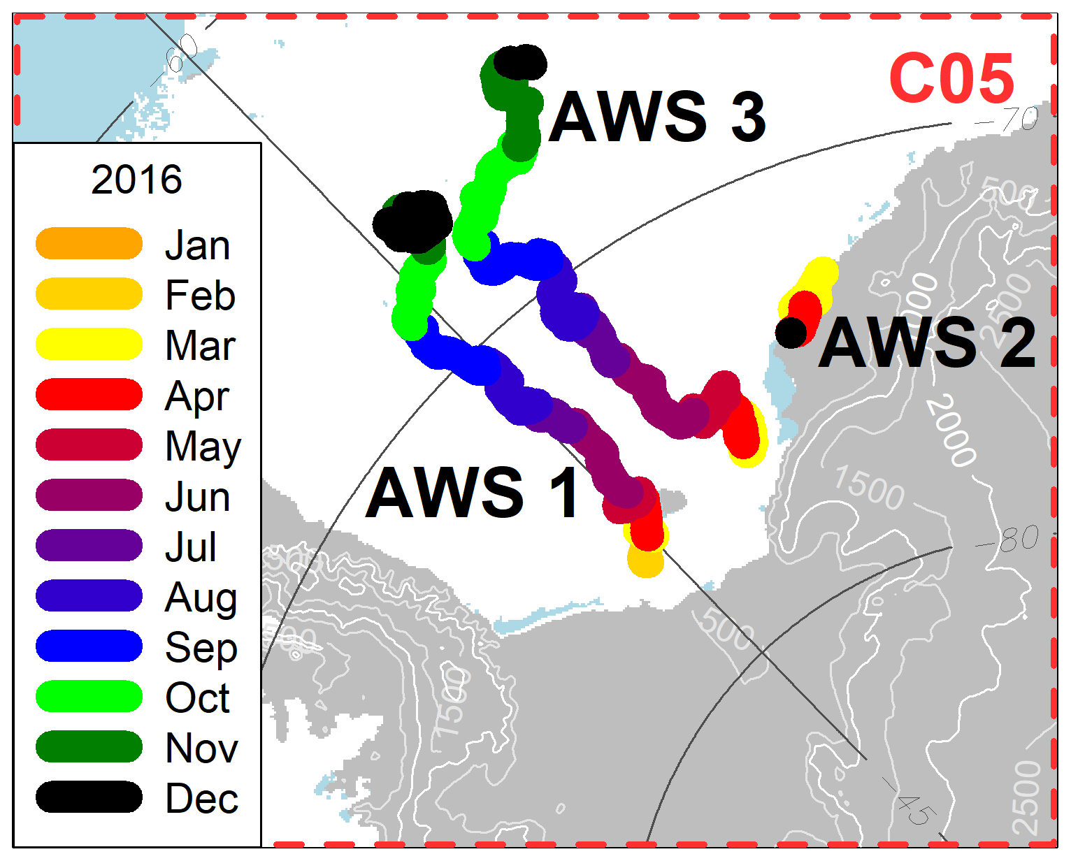
Figure 2 Overview of tracks of the three AWS buoys inside the C05 domain. Topography and sea ice concentration as in Fig. 1.

2.4 Radio soundings

To assess the model performance over the whole atmosphere, radio sounding (RS) data were downloaded from the University of Wyoming (http://weather.uwyo.edu/upperair/sounding.html, last access: 31 March 2020). The location of RSs are shown in Fig. 1 (diamonds), and detailed information is given in Table 5. Some RSs had an unrealistic pressure value at a given height. To remove these, we checked whether or not the deviation from the mean pressure was bigger than 3 times the standard deviation for that height. This removed only 2 %–3 % of the RSs. Further, we only selected RSs done at either 00:00 UTC for Amundsen–Scott and Novolazarevskaya or 12:00 UTC for Halley, Marambio, Neumayer, and Rothera, because these were the only times when the RSs were done regularly.

Table 5 Information on radio sounding stations. Observation (Obs) at UTC indicates the hour when the sounding was done. Interval shows the usual time difference between the radio soundings (for 85 % of all radio soundings). N indicates the number of radio soundings during 2002–2016.

2.5 Wind lidar

In the austral summer 2015/16 we conducted in situ measurements in the Weddell Sea region. We installed a Doppler lidar onboard the RV Polarstern and measured vertical profiles of horizontal wind speed and direction from 24 December till 30 January. In Zentek et al. (2018) we compared the measurements to radio soundings and ship measurements and found a bias (root-mean-square deviation) of approx. 0.1 (1) m s⁻¹ for wind speed and 1 (10)^∘ for wind direction, respectively. Lidar wind profiles are available with a vertical resolution of 10 m and with a temporal resolution of ca. 15 min. For the comparison, profiles were average to hourly values and 50 m height resolution (Zentek and Heinemann, 2019a).

For the purpose of comparisons we also set up another model domain with a 1 km resolution and nested it inside the 5 km domain. We ran both with the original settings (C01/C05) and changed turbulence parameters (T01/T05) for the measuring period (see Table 1).

2.6 Methods

For the comparison of CCLM with AMPS and ERA-Interim data, the latter were interpolated bilinearly to the CCLM grid points. For the comparisons to measurements (MS, AWS, RS, and lidar) the nearest neighbouring grid point of CCLM was selected. For surface stations, the CCLM temperature was corrected with 1 K per 100 m for the height difference between the station and the respective grid point (see Tables 4 and 5 for information on grid point heights and difference to the actual station height).

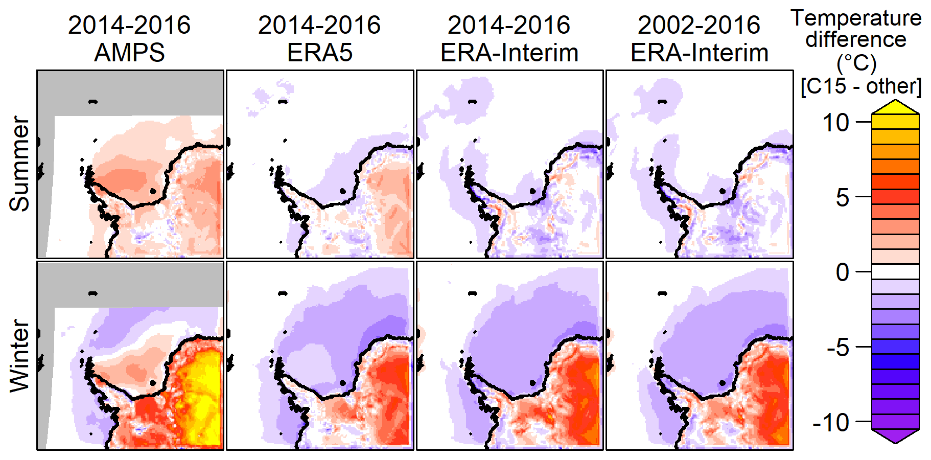
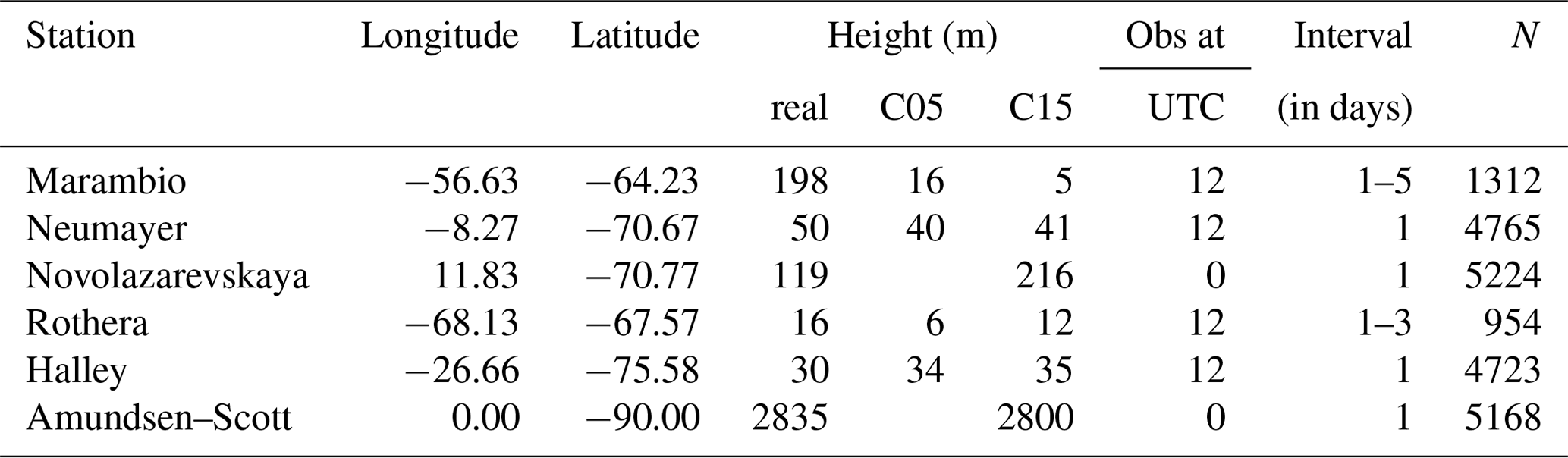
Figure 3 The 2 m temperature difference (C15 minus AMPS, ERA5, and ERA-Interim) for the years 2014–2016 and 2002–2016. Summer (October–March, top) and winter (April–September, bottom) are shown separately. The grey area is outside the AMPS domain.

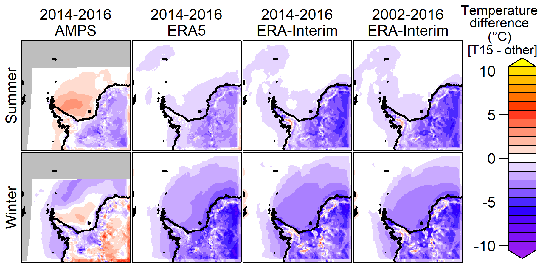
Figure 4 As Fig. 3 but for T15.

Figure 5 As Fig. 3 but for 10 m wind speed.

For the radio sounding comparisons, we made a vertical linear interpolation of model and radio sounding data to the same pressure level (equidistant, every 50 hPa). Only data at a certain pressure level were analysed if the number of measurements was more than half of the median of the number of observations over all heights. Prior to the calculation of the correlation for temperature, monthly means were subtracted to remove influence from the seasonal cycle.

In the case of the three AWS buoys on ice floes, the wind speed was measured at a height of approximately 2 m. We therefore assumed a logarithmic wind profile and neutral stability with a roughness length of 0.001 m and thus scaled CCLM 10 m wind speed by a factor of 0.825 in order to calculate the 2 m wind speed. For the AWSs over land no correction was applied as the height of sensors was uncertain or unknown.

For the lidar comparisons we interpolated model, reanalyses, and lidar data to an equidistant grid (height every 50, up to 1000 m). As ERA-Interim only has output every 6 h, we did not interpolate linearly in between, in order to have a sharper distinction to ERA5. Further, note that the lidar data are on average over 1 h around every full hour, which removes small-scale variability as the single measurements were done approximately every 15 min for 1–2 min. This makes it better comparable to the simulation data because although the output is instantaneous, it is unlikely that it shows turbulence on such a small scale as it always represents the wind average over the whole model grid box.

The wind comparisons are based on the magnitude of wind speed and the wind direction (no vector differences) unless stated otherwise. For wind direction we always assume a maximal possible difference of 180^∘ and removed cases where wind speed is lower than 0.5 m s⁻¹. We compute the root-mean-square error (RMSE) and use the Pearson correlation coefficient (Corr) for temperature and wind speed but use an adapted version for angular variables (Jammalamadaka and Sarma, 1988) (circ.Corr) for wind direction.

3 Comparison with AMPS and ERA

Although a verification with measurements is preferable, due to the small number of stations in polar regions this is not possible for the whole model domain. A comparison to other simulations is therefore an addition to the evaluation, although it has its limits. Gossart et al. (2019) found that in some respects different reanalyses (including ERA5 and ERA-Interim) differ greatly between each other in Antarctica, and thus comparisons of CCLM with these data should not be seen as a validation.

In this analysis the near-surface variables of CCLM are compared with ERA-Interim, ERA5, and AMPS. We computed monthly mean values over the period of 2002–2016 of 2 m temperature and 10 m wind speed. As the data sets of AMPS (with the latest configuration) do not cover the whole period, we selected the years 2014–2016 for the main comparisons. For ERA-Interim we show both time periods.

The 2 m temperature differences for C15 for the winter (April–September) and summer (January–March and October–December) are shown in Fig. 3. The differences for summer are small. For winter C15 is 1–3 K colder over sea ice than ERA5 and ERA-Interim, but this is still a small difference. Over the East Antarctic Plateau (topography approximately higher than 2 km), a large temperature difference of up to 8 K compared to ERA5/ERA-Interim and up to 15 K compared to AMPS is visible during winter.

Figure 6 Comparison for Halley of (a) 2 m temperature, (b) 10 m wind speed, and (c) 10 m wind direction for station measurements (black), C15 (blue), and T15 (green) during January 2016. Vertical grey lines indicate the restart of the daily simulations.

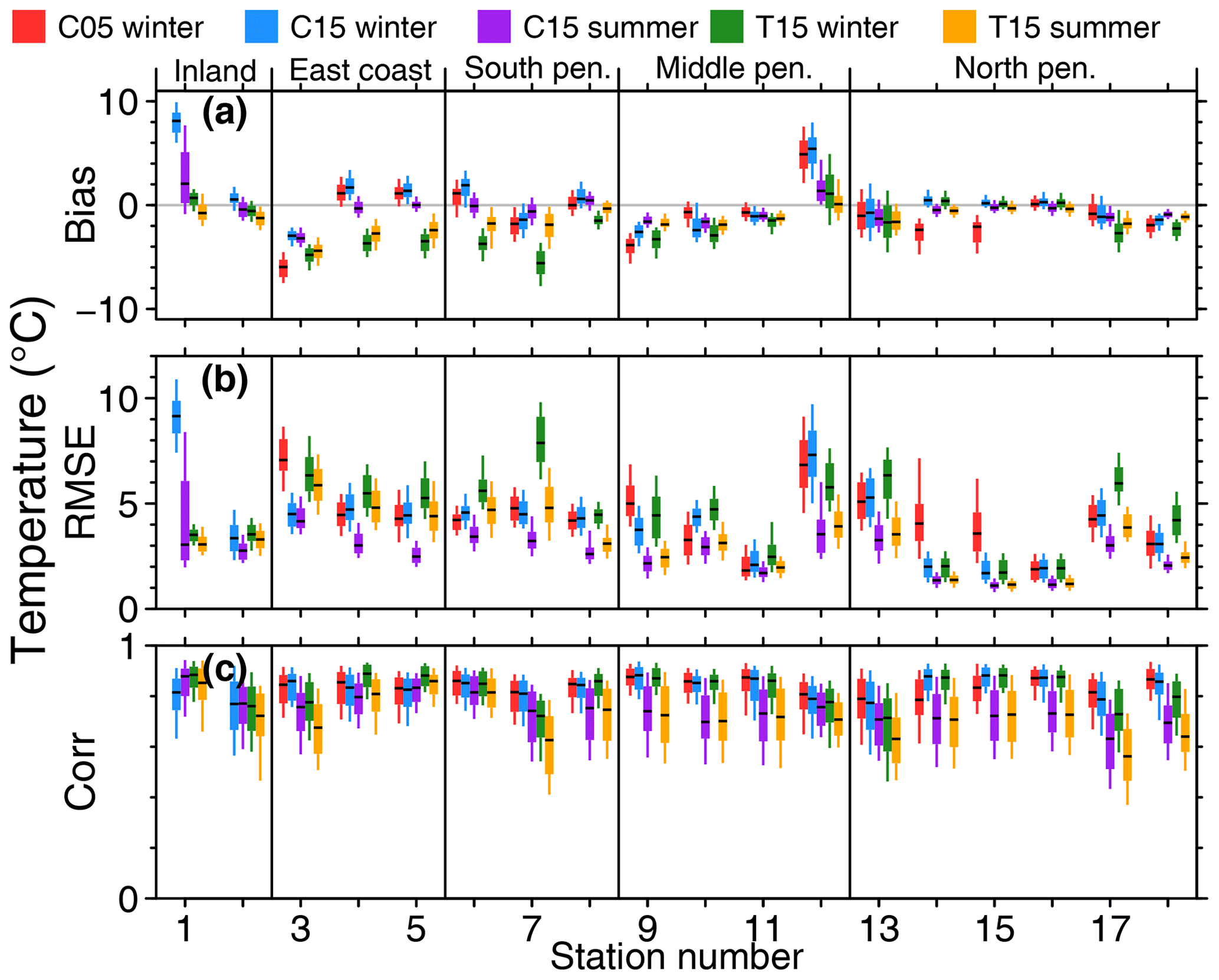
Figure 7 CCLM (a) 2 m temperature bias, (b) RMSE, and (c) correlation for C05, C15, and T15 for different surface stations (see Table 4). Boxes indicate the 25 %∕75 % quantiles, and whiskers indicate the 10 %∕90 % quantiles; the median is indicated by a black line inside the box. Statistics (bias, RMSE, and correlation) are calculated for every month.

The study by Gossart et al. (2019) showed the largest differences in mean temperature between reanalyses over the interior of Antarctica during winter (approx. 8 K) and that ERA and ERA-Interim are warmer than the observations. An evaluation of AMPS (Fig. A1 in Bromwich et al., 2005) showed only a small bias (down to −3 K) of AMPS in the interior of Antarctica. Verifications using surface and radio sounding data (shown in Sect. 4) confirmed that C15 is too warm over the plateau and that this could be attributed to a too strong mixing in the surface boundary layer. This was the reason for changing the turbulence parametrization (T15).

As the change in turbulence parameters allows for more stable atmospheric boundary layer, T15 is overall colder than C15 near the surface, but this influence is very weak during summer or over the sea ice. The 2 m temperature differences for T15 are shown in Fig. 4. Over land and especially over the East Antarctic Plateau the strong difference in winter present in C15 is reduced in T15 compared to AMPS and even turns into a negative difference compared to ERA5 and ERA-Interim. Figure 5 shows the 10 m wind speed differences for C15 for the summer and winter period. The differences for T15 are very similar (Fig. S1 in the Supplement). Compared to ERA5 and ERA-Interim, C15 shows stronger winds (up to 5 m s⁻¹ faster) over the Antarctic Peninsula and in the katabatic wind areas. For the winter period C15 simulates slightly weaker winds over the northern part of the sea ice when compared to ERA5 and ERA-Interim, which may be a result of the different sea ice parametrizations. The difference in C15 compared to AMPS is mainly negative over the ice sheet and slightly positive for the Filchner–Ronne Ice Shelf. The C05 simulation (not shown) shows slightly higher 10 m winds (1 m s⁻¹) compared to the C15 simulation and slightly lower (1 K) 2 m temperature.

Figure 8 As Fig. 7 but for 10 m wind speed.

Figure 9 As Fig. 7 but for 10 m wind direction.

Overall the C15 simulation is comparable to ERA5, ERA-Interim, and AMPS model data except for the large temperature difference (C15 warmer) during winter over high topography. When using the modified turbulence scheme, the difference with respect to the ERA is reversed (T15 colder), but it becomes more similar to AMPS.

4 Comparison to observations

4.1 AWSs and surface stations

To further investigate the differences between CCLM and other simulations from the last section, we compared C15 and T15 with surface measurements. The selection of stations was done after a quality check and using only stations with sufficient record length. In addition the stations should represent typical areas of the Weddell Sea region. The locations of the selected stations are shown in Fig. 1, and detailed information is given in Table 4.

A 10 d comparison of measurements and CCLM model output at the station Halley is shown in Fig. 6. Both C15 and T15 capture the daily cycle of temperature, but T15 underestimates the temperature during some nights with low wind speeds. Wind speed and direction of C15 and T15 are similar and agree very well with the measurements. Only during the first day is the change in wind direction different, but the wind speed for this day is also very low.

For the full comparison of C05, C15, and T15 with all stations we calculated monthly bias, RMSE, and correlation for winter and summer separately. Statistics for 2 m temperature are shown in Fig. 7.

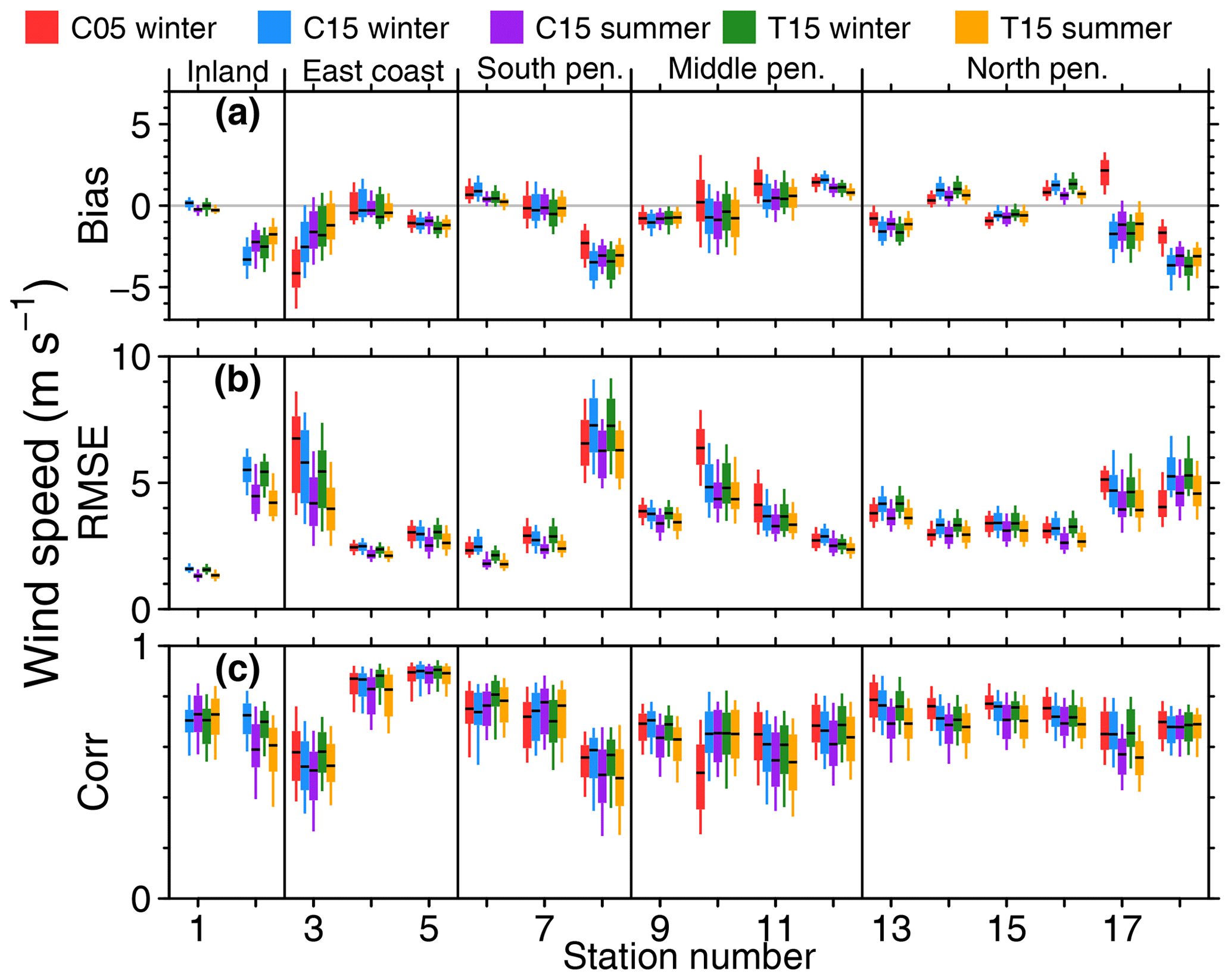
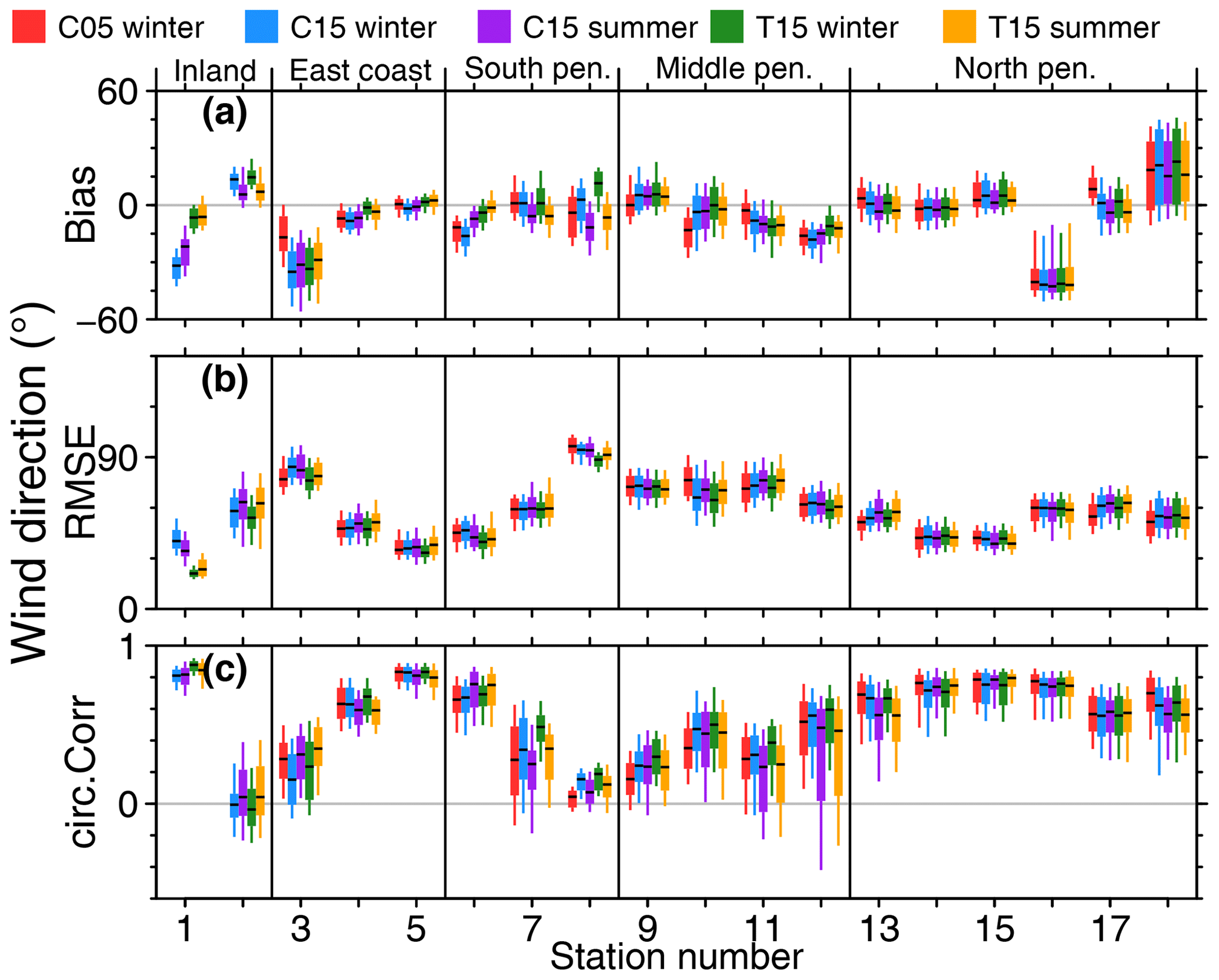
The problem of the temperature bias of C15 over the plateau can be demonstrated for the Amundsen–Scott data (no. 1). The +8 K bias for C15 in winter is reduced to less than 1 K in the case of T15, thus showing better performance of T15. The improvement can also be seen for summer. On the other hand, a small cold bias is present for T15 for the coastal region. The statistics for 10 m wind speed (Fig. 8) and direction (Fig. 9) show almost no difference between C15 and T15. The reduced bias of T15 compared to C15 in wind direction for Amundsen–Scott (no. 1) is a result of better representation of the stable boundary layer in T15. This yields colder surface temperatures that allow for a stronger wind shear and thus a reduced wind direction bias.

At AWS Union (no. 2) wind direction is almost constant with time, which results in a low correlation although the bias and RMSE are comparable to other stations. For AWS Fossil (no. 8) there are two dominant wind directions both measured and simulated, but they do not always coincide in time, and thus the RMSE is also very high.

The strong bias in wind direction for Bellingshausen (no. 16) is likely explained by the different small-scale topography around the stations, which is not captured at the model resolutions. Also, a data error at the station cannot be ruled out, as the other northern Antarctic Peninsula stations are relatively close to each other and do not show this bias. The reasons for the high bias and RMSE of wind direction for Belgrano II (no. 3) are also likely a result of small-scale topography effects.

Overall CCLM has a tendency to perform slightly better during summer, and differences between the model runs C05, C15, and T15 are only visible in the case of 2 m temperature. When calculating daily instead of monthly bias, RMSE, and correlation, the results are similar but show a much higher variance. These statistics are shown in Figs. S2, S3, and S4.

In Sect. 3, differences in temperature and wind speed were found compared to AMPS, ERA5, and ERA-Interim over sea ice. Observations over sea ice are rare, but the three drifting AWS buoys allow for a comparison of a full yearly cycle for the year 2016. All buoys were deployed in January 2016 near the east coast of the Weddell Sea but at different positions. The no. 1 and 3 buoys drifted from their original position near the coast of northwards out of the Weddell Sea and no. 2 stayed near the east coast (see Fig. 2). An overview of the measurements for the AWS 3 buoy is shown in Fig. 10. The seasonal cycle of temperature is captured by all model runs, and wind speed and direction agree well.

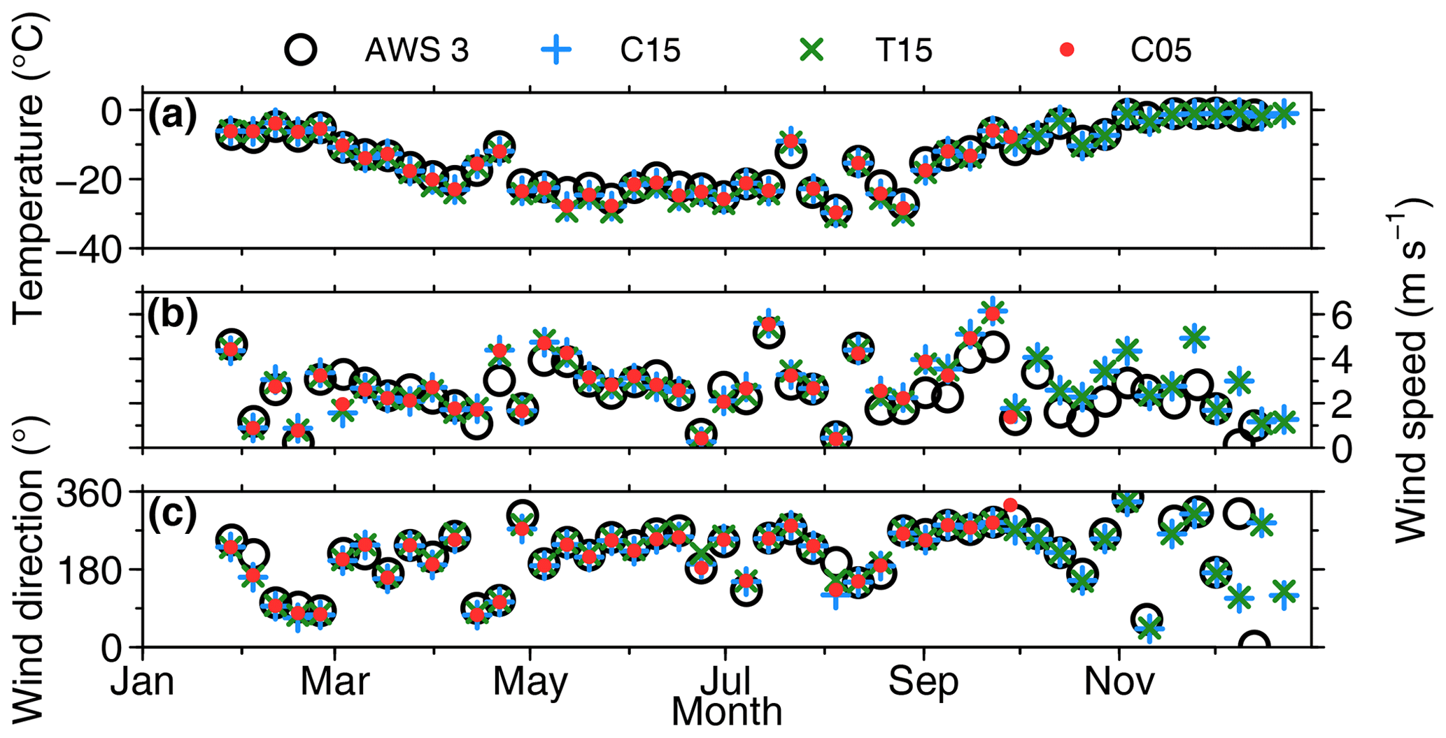
Figure 10 (a) Weekly temperature, (b) wind speed, and (c) wind direction in 2016 for AWS 3 buoy in black (see Fig. 2), C15 (blue), T15 (green), and C05 (red). The weekly mean was computed for zonal and meridional winds.

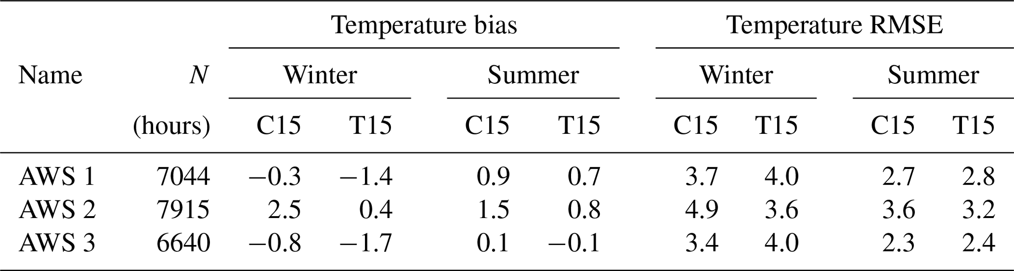
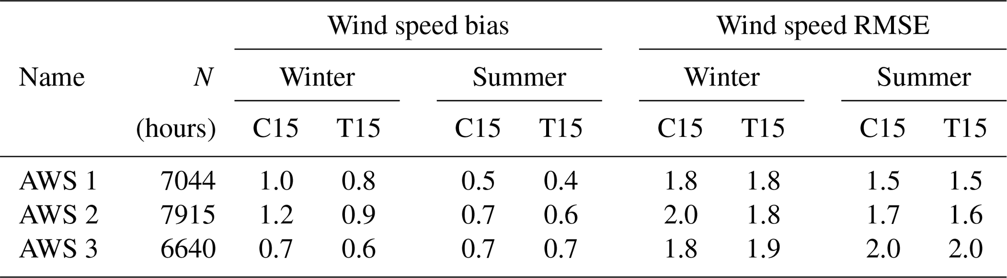
The bias and RMSE of CCLM based on hourly temperature and wind speed for all AWSs are given in Tables 6 and 7. Overall AWS 1 and AWS 3 show similar statistics as both drifted relatively synchronously northwards, while AWS 2 stayed close to the coast north of the station Halley (no. 4). C15 shows a temperature bias of $-\mathrm{0.3}/-\mathrm{0.8}$ K for AWS 1/AWS 3 during winter, while T15 shows a slightly larger bias of $-\mathrm{1.4}/-\mathrm{1.7}$ K. This is not as high as the previously seen cold bias over sea ice during winter of CCLM compared to ERA-Interim and ERA5 of −2 K for C15 and −3 K for T15 (see Figs. 3 and 4). The RMSE is approx. 4 (3) K during summer (winter). For wind speed the RMSE is around 1.5 to 2 m s⁻¹, and biases are equal to or smaller than 0.7 m s⁻¹ during summer and a little higher, around 1 m s⁻¹, during winter (Figs. S5 and S6).

Table 6 CCLM temperature bias and RMSE for the three AWS buoys (see Fig. 2). N indicates the number of data points (hours) in 2016. Winter months are April–September, and summer months are January–March and October–December.

Table 7 As Table 6 but for wind speed.

4.2 Radio soundings

The location of the radio soundings are shown in Fig. 1 as diamonds. Note that Novolazarevskaya is very close to the model boundary (eight grid points), and CCLM may be partly influenced by the ERA-Interim boundary data. The radio soundings are done regularly at 00:00 UTC (6 h after model start) for Novolazarevskaya and Amundsen–Scott and 12:00 UTC (18 h after model start) for Marambio, Neumayer, Rothera, and Halley.

To address the differences between C15 and T15, a comparison of the mean temperature for the lowest 1 km of the atmosphere is shown in Fig. 11. The changed turbulence parametrization only influences the cases of strong surface inversions. For Amundsen–Scott (f) there is a clear improvement in T15 for the mean SBL structure during winter and also a slight improvement during summer. Similar but weaker improvements can be seen for the eastern Weddell Sea – Halley (e) and Neumayer (b). However, for Novolazarevskaya (c) and Rothera (d) a stronger bias in the lowest 100 m is present for T15.

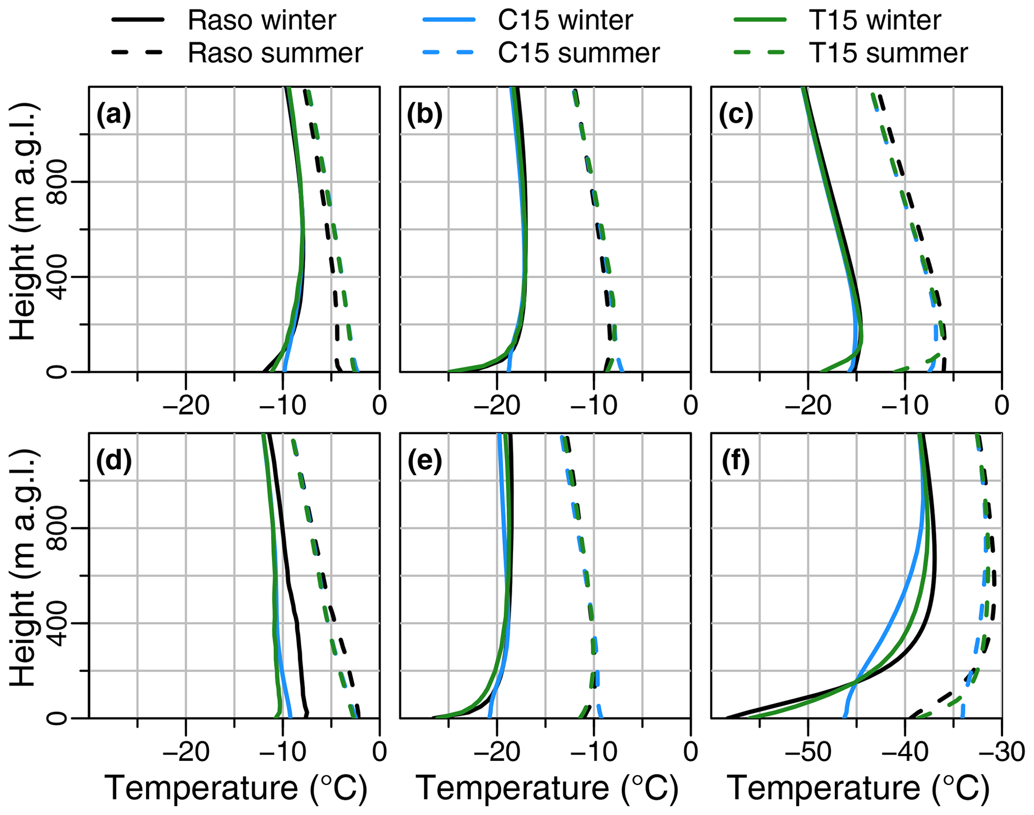
Figure 11 Mean temperature of radio sounding (Raso; black), C15 (blue), and T15 (green) during winter (solid line) and during summer (dashed line) for the stations (a) Marambio, (b) Neumayer, (c) Novolazarevskaya, (d) Rothera , (e) Halley, and (f) Amundsen–Scott. Note the different range on the x axis for (f) Amundsen–Scott. The abbreviation a.g.l. is short for “above ground level”, meaning above the surface.

The whole profiles of the temperature statistics (Fig. 12) show almost no bias except below 800 hPa, and the RMSE is around 1 K in the upper troposphere for the coastal stations. The bias is slightly lower for C05 (only winter) and for C15 in summer. The correlations are larger than 0.8. These results are similar to the findings of Souverijns et al. (2019), which show a mean average error of 0.5 to 1.4 K. For Amundsen–Scott (f) a large positive bias and a large RMSE is present in the lowest layers, which is most pronounced in winter. While for the winter the RMSE and the correlation above 500 hPa are comparable to the coastal stations, a larger RMSE and correlations of less than 0.75 are present above 500 hPa during summer. The higher resolution of C05 yields only slight improvements for Marambio (a) and Rothera (d) at the Antarctic Peninsula, where the influence of the topography is larger than at the other stations. We did not include T15 in Fig. 12 as the statistics were almost identical to C15 with the exception of the lowest levels for Amundsen–Scott.

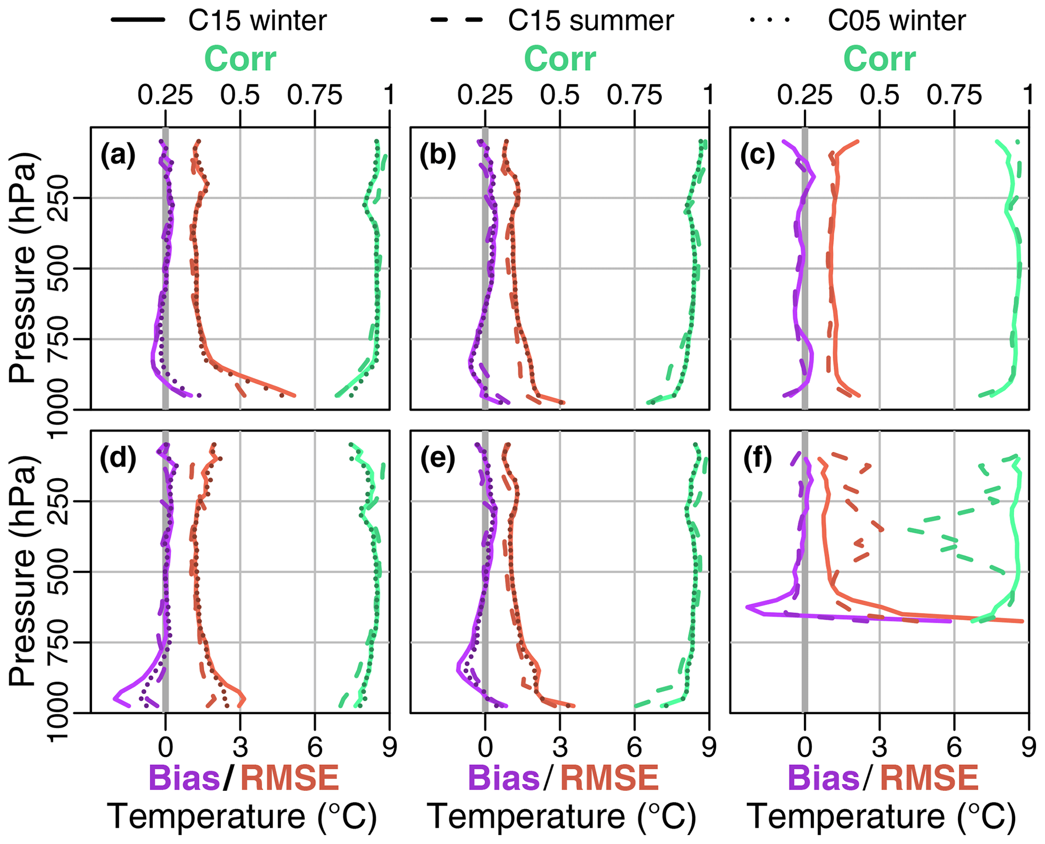
Figure 12 Temperature bias, RMSE (bottom axes), and correlation (top axes) of C15 during winter (solid line), C15 during summer (dashed line) ,and C05 during winter (dotted line) for the stations (a) Marambio, (b) Neumayer, (c) Novolazarevskaya, (d) Rothera, (e) Halley, and (f) Amundsen–Scott.

Above the surface inversion, differences for C05, C15, and T15 and the summer and winter season are relatively small, with only a minor exception of a small increase in RMSE above 500 hPa for Amundsen–Scott (f) during summer.

For the comparison of wind speed (Fig. 13) and direction (Fig. 14) we excluded T15 again, as it was almost identical to C15. The bias is again almost 0 except near the surface. The RMSE for wind speed is around 3 to 4 m s⁻¹ and slightly lower during summer. Bias and RMSE are largest for Marambio (a) and Rothera (d) in the lowest 200 hPa, and as for the temperature C05 yields slight improvements for these stations. Souverijns et al. (2019) found a mean average error for wind speed of 2.1 to 3.6 m s⁻¹ for all seasons. The RMSE for wind direction is around 50^∘ near the surface and reduces with height to 20^∘ at 250 hPa, except for Amundsen–Scott (f) where it stays around 50^∘.

Figure 13 Like Fig. 12 but for wind speed.

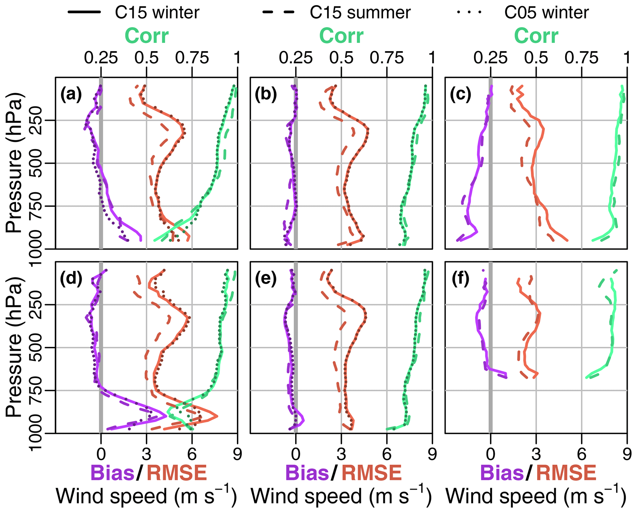
4.3 Wind lidar

Wind profile measurements from lidar data are available for 24 December 2015 to 30 January 2016. We selected two case studies for comparisons. The first one features the occurrence of three low-level jets (LLJs) during a night and the following morning. The second case study gives an overview of the differences and similarities between lidar measurements and simulations during a 10 d period.

4.3.1 Overall statistics

We also computed the overall statistics for all available lidar measurements (see Table 8). The different CCLM runs are very similar, with no or only very small bias in wind speed and a RMSE of around 2 m s⁻¹. For wind direction there was a small bias of −5^∘ present and a RMSE of 30^∘. ERA5 and ERA-Interim show similar values. This good agreement could stem partially from the fact that the radio soundings of the ship (2–3 d⁻¹) are assimilated in ERA5 and ERA-Interim, which show also good agreement with the lidar data (Zentek et al., 2018). The computation of the statistics for different heights showed that the wind speed RMSE of CCLM is largest around a height of 1000 m, while the RMSE of ERA5 and ERA-Interim is mostly constant with height (Fig. S7).

4.3.2 Case study A

During the night from 16 to 17 January 2016 the RV Polarstern operated in a polynya in the lee of the iceberg A23 (see Fig. 1). Three LLJ events were observed with the lidar (Fig. 15). The first LLJ occurred between 00:00 and 02:00 UTC (LLJ1). The LLJ between 06:00 and 08:00 UTC (LLJ2) was captured by the radio sounding at 07:00 UTC (Zentek et al., 2018), and the wind maximum between 10:00 and 14:00 UTC (LLJ3) was also measured by a radio sounding at heights of 800 to 1000 m at 12:00 UTC. While the 6-hourly ERA-Interim data cannot reproduce the structure and evolution of the wind field of the lidar measurements, the hourly ERA5 data capture LLJ2 and LLJ3, which is likely explained by the assimilation of radio sounding data. However, the LLJ wind speeds are underestimated, and LLJ1 is missing in ERA5. The CCLM simulations (nested in ERA-Interim) show that the increase in resolution yields increased wind speeds particularly for LLJ3, but the height of the LLJ is too low. An indication of LLJ1 is seen in the CCLM simulations, but the wind speed is underestimated. The overall pattern of the wind direction field is well reproduced by all CCLM simulations. Since the position of the ship was not stationary for this period, we also tested for a dependency on the chosen grid point of the model, by choosing one grid point over the iceberg A23 and one in the middle of the open polynya instead of the ship location. This had only a small effect, and we therefore concluded that all the changes and patterns are mostly time and height dependent.

Figure 14 Like Fig. 12 but for wind direction.

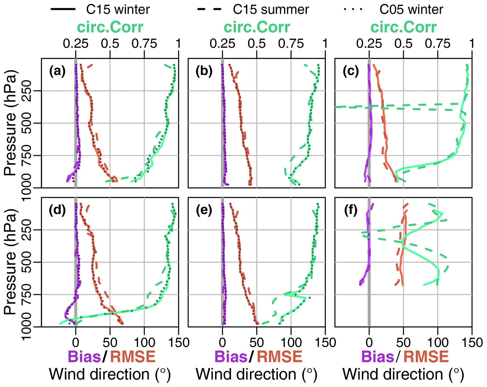
Table 8 Bias and RMSE for wind speed and direction compared to lidar measurements during December 2015 and January 2016.

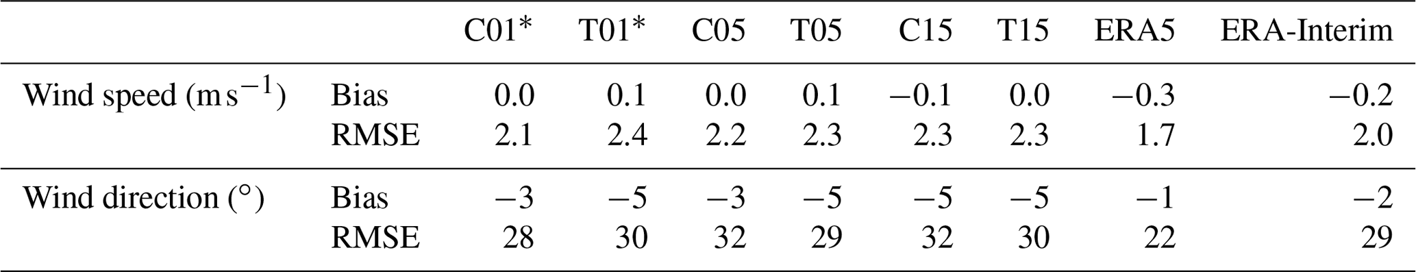
^∗ The runs with 1 km resolution were not performed for the whole period but only for 37 and 25 d (out of 39 d) for T01 and C01, respectively.

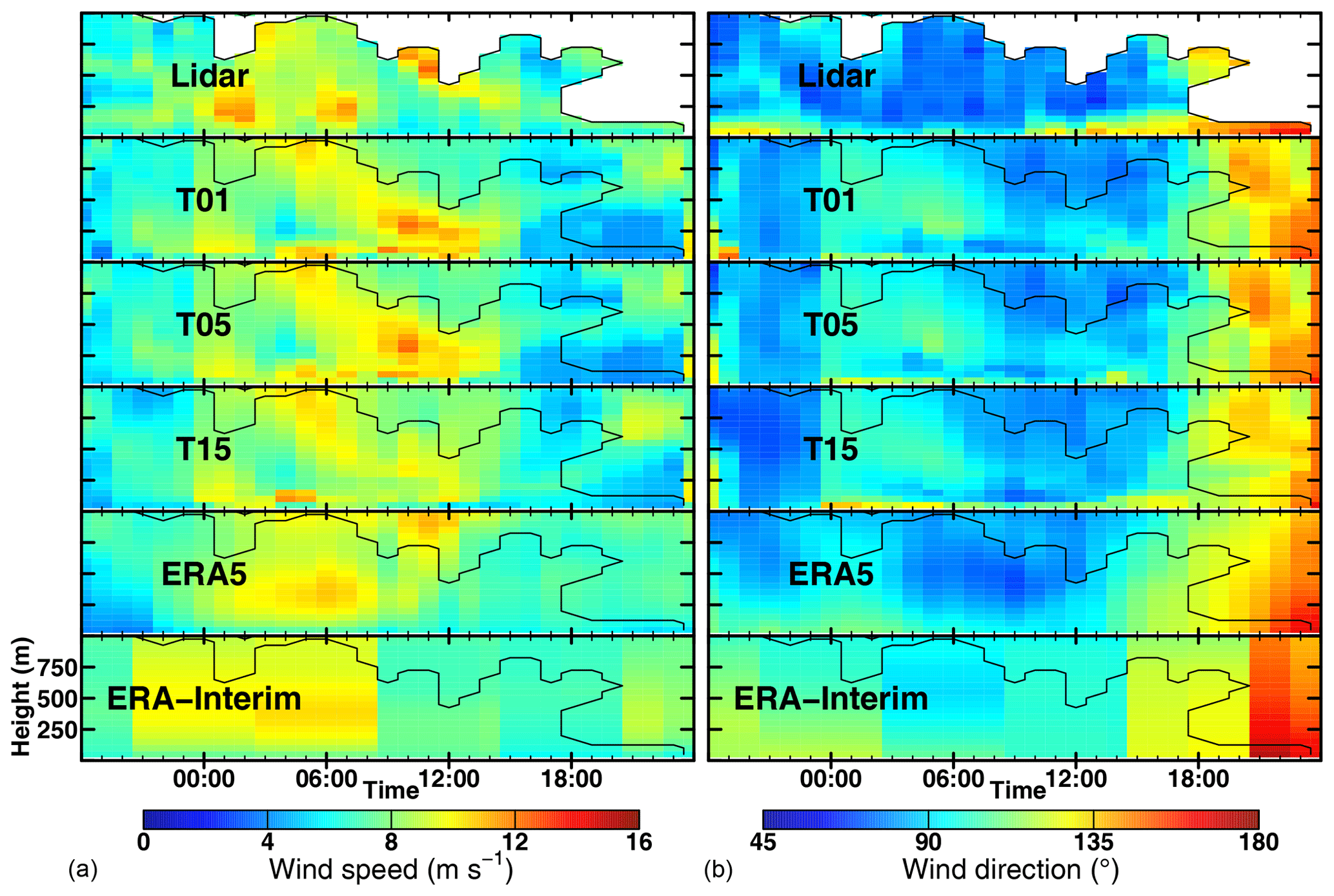
Figure 15 Time–height cross sections for (a) wind speed and (b) direction for 16 January 2016 18:00 UTC to 17 January 2016 12:00 UTC.

4.3.3 Case study B

From 20 to 30 January 2016 RV Polarstern was navigating around the area of the Brunt Ice Shelf (see Fig. 1). The days show a broad variety of different wind patterns (Fig. 16) ranging from no wind (on the 21st) to wind speeds exceeding 20 m s⁻¹ (on the 29th) and also featuring vertically inhomogeneous winds both in speed and direction (on the 24th–26th). On the scale of days, T15, ERA5, ERA-Interim, and the lidar show the same evolution of the wind field. On smaller scales, CCLM and the lidar show more detail, but CCLM does not always agree well with the lidar (e.g. on the 26th). ERA5 agrees well with the lidar data and sometimes even catches the small-scale details of measured wind patterns (e.g. on the 27th). T05 and T01 are very similar to T15, with only little-increased wind speeds (Fig. S8).

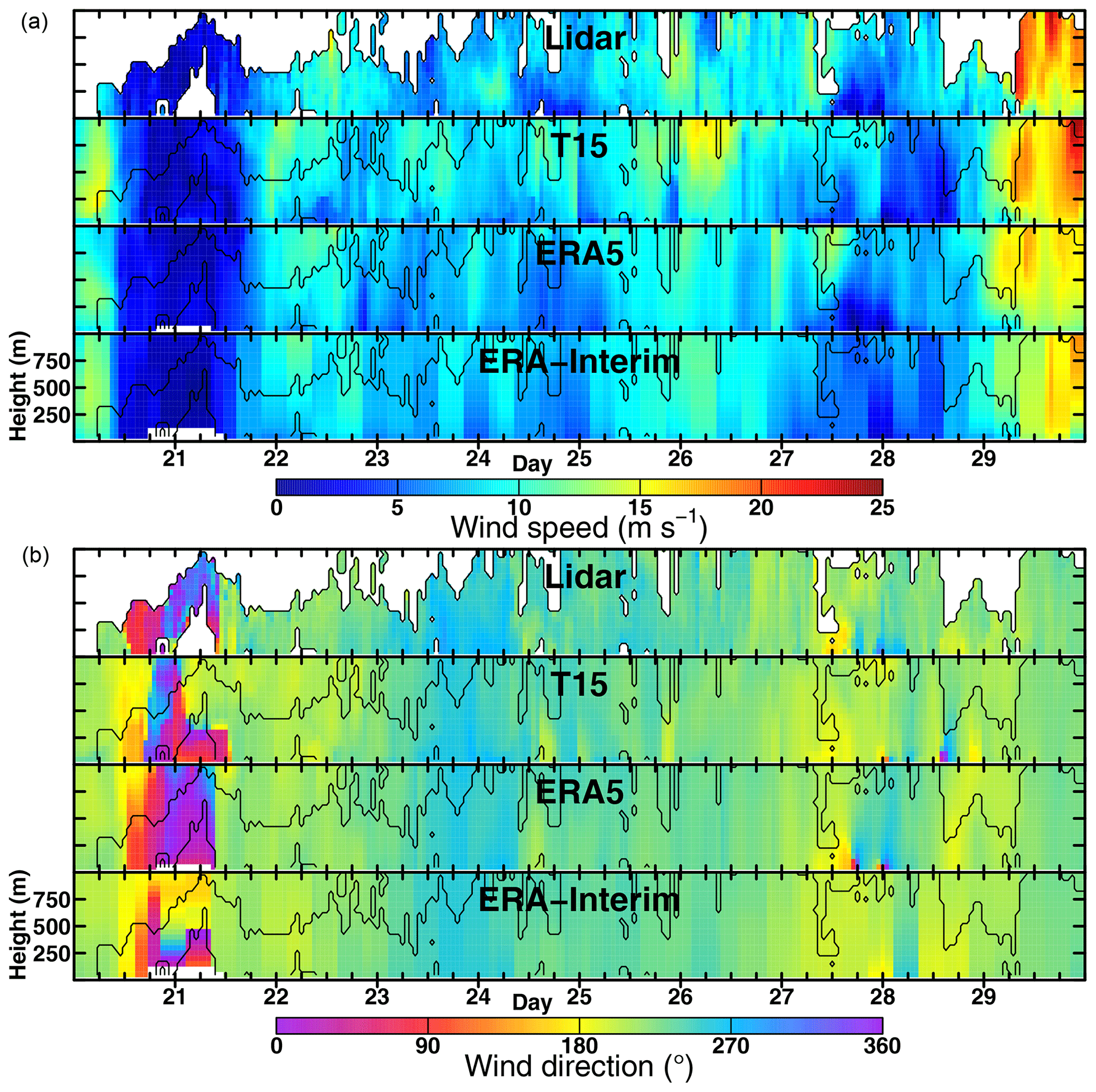
Figure 16 Time–height cross sections for (a) wind speed and (b) direction for 20 January 00:00 UTC to 30 January 00:00 UTC.

If we presume that the lidar measurements are representative of the winds in the whole area that is covered by the model grid box, this case study gives a good impression of how reliable reanalyses and models are on those scales; e.g. for a simulated LLJ we cannot always assume that a LLJ was really present, even if the overall RMSE is shown to be smaller than 3 m s⁻¹.

5 Summary

We used the nonhydrostatic model COSMO-CLM (CCLM) in forecast mode and nested in ERA-Interim data to produce a long-term hindcast (2002–2016) for the Weddell Sea region with resolutions of approximately 15 and 5 km and two different turbulence parametrizations. Sea ice concentration is prescribed from satellite data, and a thermodynamic sea ice model is used. In this paper we evaluated the performance of the model in terms of temperature, wind speed, and direction using data from Antarctic stations and AWSs over land and sea ice. Comparisons to the AMPS model and reanalyses data showed good agreement, except for a large difference in surface temperature over the Antarctic Plateau. The warm bias is also found in comparison to measurements at the Amundsen–Scott station (surface and radio sounding), where the reference run C15 showed a strong warm bias near the surface (+8 K). This bias was removed in the second run T15 by adjusting the turbulence parametrization, which results in a more realistic representation of the surface inversion over the Antarctic Plateau. But this caused also a small cold bias (down to −4 K) for other surface stations located on ice shelves in the eastern Weddell Sea. A comparison with measurements over the sea ice of the Weddell Sea done by three AWS buoys for 1 year showed small biases for temperatures around ±1 K and for wind speed of 1 m s⁻¹.

Comparisons with radio soundings showed a model bias around 0 for all model levels except near the surface. In general, a RMSE of 1–2 K for temperature and 3–4 m s⁻¹ for wind speed was found.

The comparison of CCLM simulations at resolutions down to 1 km with wind data from Doppler lidar measurements during December 2015 and January 2016 in the southern and eastern Weddell Sea yielded almost no bias in wind speed and a RMSE of ca. 2 m s⁻¹. For wind direction the bias was ca. −5^∘ with a RMSE of around 30^∘. Overall, CCLM is able to produce realistic evolution and structures of the wind in the ABL, but for specific events like LLJs differences in the timing and locations of the LLJs occur.

6 Conclusions and outlook

CCLM shows a good representation of temperature and wind for the Weddell Sea region. The adjustment of the turbulence parametrization for very stable conditions is important for the realistic representation of the surface inversion over the Antarctic Plateau. Since verification data for simulations are rare in the Antarctic, new types of measurements like Doppler lidar or controlled meteorological balloons (Hole et al., 2016) can give additional insights into the performance of atmospheric models. For the comparisons of CCLM with ship-based Doppler lidar in the present study the benefit of CCLM compared to ERA5 is small due to the facts that the data from the ship were assimilated in the reanalysis and effects of topography were small. A larger benefit is seen for polynya areas and the Antarctic Peninsula with small-scale topography. The YOPP (Year of Polar Prediction) project will lead to more and enhanced observational data, which can be used for further verifications in the future. Future work with CCLM will be the study of atmosphere–ice–ocean interactions processes and quantification of sea ice production in polynyas.