the Creative Commons Attribution 4.0 License.
the Creative Commons Attribution 4.0 License.
 | 03 Apr 2020
Prediction of source contributions to urban background PM10 concentrations in European cities: a case study for an episode in December 2016 using EMEP/MSC-W rv4.15 and LOTOS-EUROS v2.0 – Part 1: The country contributions
Hilde Fagerli
Michael Schulz
Alvaro Valdebenito
Richard Kranenburg
Martijn Schaap
A large fraction of the urban population in Europe is exposed to particulate matter levels above the WHO guideline value. To make more effective mitigation strategies, it is important to understand the influence on particulate matter (PM) from pollutants emitted in different European nations. In this study, we evaluate a country source contribution forecasting system aimed at assessing the domestic and transboundary contributions to PM in major European cities for an episode in December 2016. The system is composed of two models (EMEP/MSC-W rv4.15 and LOTOS-EUROS v2.0), which allows the consideration of differences in the source attribution.
We also compared the PM10 concentrations, and both models present satisfactory agreement in the 4 d forecasts of the surface concentrations, since the hourly concentrations can be highly correlated with in situ observations. The correlation coefficients reach values of up to 0.58 for LOTOS-EUROS and 0.50 for EMEP for the urban stations; the values are 0.58 for LOTOS-EUROS and 0.72 for EMEP for the rural stations. However, the models underpredict the highest hourly concentrations measured by the urban stations (mean underestimation of 36 %), which is to be expected given the relatively coarse model resolution used (0.25∘ longitude × 0.125∘ latitude).
For the source attribution calculations, LOTOS-EUROS uses a labelling technique, while the EMEP/MSC-W model uses a scenario having reduced anthropogenic emissions, and then it is compared to a reference run where no changes are applied. Different percentages (5 %, 15 %, and 50 %) for the reduced emissions in the EMEP/MSC-W model were used to test the robustness of the methodology. The impact of the different ways to define the urban area for the studied cities was also investigated (i.e. one model grid cell, nine grid cells, and grid cells covering the definition given by the Global Administrative Areas – GADM). We found that the combination of a 15 % emission reduction and a larger domain (nine grid cells or GADM) helps to preserve the linearity between emission and concentrations changes. The nonlinearity, related to the emission reduction scenario used, is suggested by the nature of the mismatch between the total concentration and the sum of the concentrations from different calculated sources. Even limited, this nonlinearity is observed in the , , and H2O concentrations, which is related to gas–aerosol partitioning of the species. The use of a 15 % emission reduction and of a larger city domain also causes better agreement on the determination of the main country contributors between both country source calculations.
Over the 34 European cities investigated, PM10 was dominated by domestic emissions for the studied episode (1–9 December 2016). The two models generally agree on the dominant external country contributor (68 % on an hourly basis) to PM10 concentrations. Overall, 75 % of the hourly predicted PM10 concentrations of both models have the same top five main country contributors. Better agreement on the dominant country contributor for primary (emitted) species (70 % is found for primary organic matter (POM) and 80 % for elemental carbon – EC) than for the inorganic secondary component of the aerosol (50 %), which is predictable due to the conceptual differences in the source attribution used by both models. The country contribution calculated by the scenario approach depends on the chemical regime, which largely impacts the secondary components, unlike the calculation using the labelling approach.
- Article
(4191 KB) - Full-text XML
- Companion paper
-
Supplement
(2288 KB) - BibTeX
- EndNote


The adverse health impacts from air pollution and especially from particulate matter (PM) are a well-documented problem (e.g. Keuken et al., 2011; REVIHAAP, 2013; Mukherjee and Agrawal, 2017; Segersson et al., 2017). Furthermore, it affects crop yields (e.g. Crippa et al., 2016), visibility (e.g. Founda et al., 2016) and even the economy (e.g. Meyer and Pagel, 2017). The mass of particulate matter with an aerodynamic diameter lower than 10 µm (PM10) is an air quality metric linked to premature mortality at high exposure (e.g. Dockery and Pope, 1994). The World Health Organization (WHO) has established a short-term exposure PM10 guideline value of 50 µg m−3 daily mean that should not be exceeded in order to ensure healthy conditions (the long-term exposure guideline is 20 µg m−3 for annual mean PM10) (WHO, 2005). Although policies have been proposed and implemented at the international (e.g. Amann et al., 2011) and national (e.g. D'Elia et al., 2009) levels, European cities still suffer from poor air quality (EEA report, 2017), especially due to high PM10 concentrations. In short, to further decrease the adverse health impacts of PM in Europe, its concentrations need to be reduced further.
PM10 concentrations in the atmosphere are highly variable in space and time. Due to the relative short atmospheric life time (from some hours to days), the variability is impacted by local sources, meteorological conditions affecting dispersion, and long-range transport as well as chemical regimes controlling the efficiency of secondary formation. PM10 consists of both primary and secondary components. Primary PM10 components include organic matter (OM), elemental carbon (EC), dust, sea salt (SS), and other compounds. Secondary PM10 is comprised of compounds formed by chemical reactions in the atmosphere from gas-phase precursors. This includes various compounds such as nitrate () from nitrogen oxide (NOx) emissions, ammonium () from ammonia (NH3) emissions, sulfate () from sulfur dioxide (SO2) emissions, and a large range of secondary organic aerosol (SOA) compounds from both anthropogenic and biogenic volatile organic compounds (VOCs). The sources for PM and its precursors are numerous, but the main anthropogenic sources are the transport, industries, energy production, and agriculture. The main natural sources are composed of forest fires, mineral dust, and sea salt. The main sink is the wet deposition. The dry deposition can also be important and depends on the type of land surface such as grass, tree leaves, and others and on meteorological conditions. With these components being derived from various sources, we understand the importance of reflecting properly the source contributions while using modelling for policy support.
Many studies have already focused on source–receptor relationships to calculate the transport of atmospheric pollutants, with country-to-country relationships (e.g. EMEP Status Report, 2018) but also over cities (e.g. Thunis et al., 2016, 2018). However, these studies focus on annual means, whereas information is also required on exposure from episodes which cause short-term limit value exceedances throughout Europe. Source apportionment provides valuable information on the attribution of different sources to PM10 concentrations. A country source calculation allows us to tackle the emissions from the countries responsible for the air pollution episode. Two distinct methodologies have been compared in this study. Indeed, the country source contribution presented hereafter is performed by two regional models, the EMEP/MSC-W model (Simpson et al., 2012) and LOTOS-EUROS (Manders et al., 2017).
The EMEP calculations use a reduced anthropogenic emission scenario and compare it to a reference run where no changes are applied. It is also known as the scenario approach. With such a simulation comparison, the simulation with reduced emissions over a source region (e.g. a country) allows us to highlight the impact of this source on the concentrations over a receptor, hereafter a city. Hence, the scenario approach is useful for analysing the concentration changes due to emission reductions. On the other hand, one simulation per source is needed to calculate the impact of each source, as is done on annual means for each country in each EMEP report (e.g. EMEP Status Report, 2018). The scenario approach may also lead to a nonlinearity in the calculated concentrations, i.e. a slight difference between the concentrations over a receptor and the sum of the estimated concentrations from different sources over this same receptor, as shown by Clappier et al. (2017a). Thus, the scenario approach is more appropriate for the calculation of the source contribution of the primary PM components than for nonlinear species such as the secondary components (e.g. Burr and Zhang, 2011; Thunis et al., 2019). LOTOS-EUROS traces the origin of air pollutants throughout a simulation using a labelling approach. The advantage of the labelling technique is the reduction in the computational time, in comparison with the scenario approach. It also quantifies the contribution of an emission source to the concentration of one pollutant at one given location. However, it is not designed to study the impact of emission abatement policies on pollutants concentrations (Grewe et al., 2010; Clappier et al., 2017b), and only traceable atoms can be used in labelling approach, i.e. only conserved atoms (C, N, and S), directly related to emission sources, in their different oxidation states. Thus, for example, the origin of ozone (O3) cannot be studied, which can be done with the scenario approach. Even if both methodologies mainly aim to answer two different questions, i.e. the emission control scenarios with the scenario approach and the attribution of concentrations from a source by the labelling technique, it is still useful to estimate the reliability of both methodologies in the estimation of the source contribution to PM10 concentrations. For example, it is important to ensure that the nonlinearity, related to the perturbation used in the scenario approach, has a limited impact on the calculated contributions and to show that both methodologies may present similar results in the country source attribution.
Both models are part of the operational country source contribution (SC) prediction system for the European cities within the Copernicus Atmosphere Monitoring Service (CAMS). This system aims at attributing country contribution to surface PM10 in European cities for 4 d forecasts. The objective of this study is to evaluate the robustness of a new system that provides forecasts of source-region-resolved PM for European cities. The evaluation of the system is focused on an event occurring between 1 and 9 December 2016, which corresponds to the first event listed from the beginning of the development of our system. To do so, the predicted PM10 concentrations are compared with observations. The simulations from both models, for the concentrations and the SC calculations, are also intercompared.
Section 2 describes the country SC system composed of the two models and the experiment. Section 3 describes the studied episode, and it presents the evaluation of both predictions in terms of PM10 concentrations. The methodology used for the SC calculations by both models is explained in Sect. 4. Then Sect. 5 gives an overview of the composition and the origin of PM10 over the cities predicted by both models and the issue regarding the nonlinearity in the chemistry related to the EMEP SC calculation. Section 6 is a comparison between the two country SC calculations. Finally, the conclusions are provided in Sect. 7.
2.1 Overview of the system
Within CAMS, a country SC product has been developed. This is a new forecasting and near-real-time source allocation system for surface PM10 concentrations and its different components over all European capitals. The predictions are available online at https://policy.atmosphere.copernicus.eu/SourceContribution.php (last access: 24 January 2020). The concentrations are calculated over the 28 EU capitals plus Bern, Oslo, and Reykjavik. Forecasts for Barcelona, Rotterdam, and Zurich are also provided. In addition to providing information about the air quality over the selected cities by focusing on PM10, this product aims at quantifying the contributions of emissions from different countries in each city (Fig. 1).
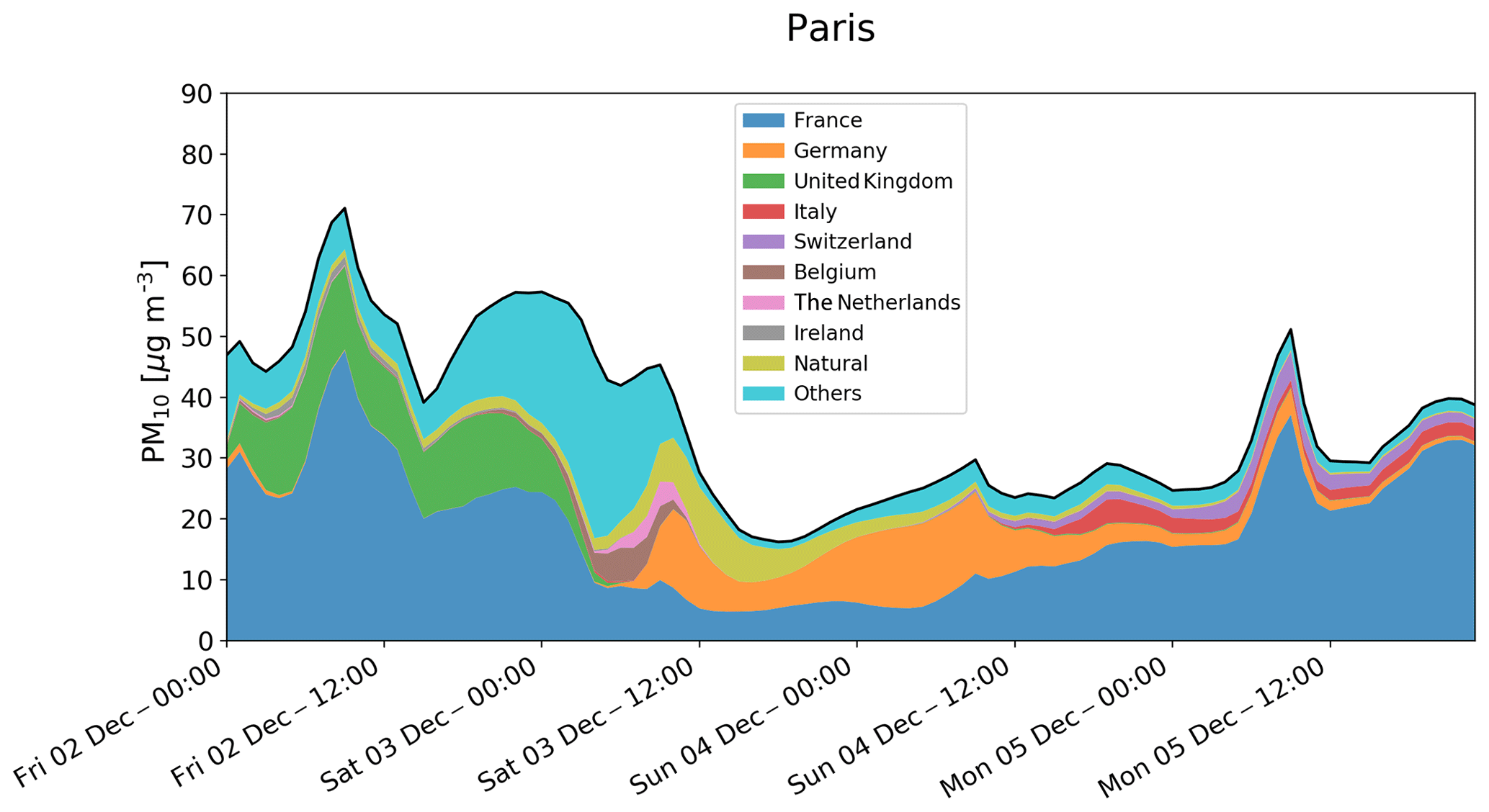
Figure 1Hourly PM10 concentrations, in micrograms per cubic metre, over Paris predicted by the EMEP model from 2 to 5 December 2016. The black curve highlights the total concentration. The eight main country contributors are plotted in addition to the natural sources and “Others”. Others contains hereafter other European countries, boundary conditions, ship traffic, biogenic sources, aircraft emissions, and lightning.
The system is composed of predictions from two regional models (the EMEP/MSC-W model and LOTOS-EUROS), using two distinct source contribution calculation methodologies. The EMEP/MSC-W chemistry transport model (Simpson et al., 2012) has been used for decades to calculate source–receptor relationships between European countries (and Russia) (e.g. EMEP Status Report, 2018), and the LOTOS-EUROS chemistry transport model (Manders et al., 2017) has also been used in several source apportionment studies over Europe, especially for PM (Hendriks et al., 2013, 2016; Schaap et al., 2013). Both models are involved in the operational air quality analysis and forecasting for Europe in the CAMS regional ensemble system (Marécal et al., 2015) and for China (Brasseur et al., 2019). For the simplicity of the reading, the EMEP/MSC-W model is hereafter referred to as the EMEP model.
Both models are Eulerian models, but there are differences between these two models such as the calculation of the planetary boundary layer (PBL) and of the advection, the vertical resolution. There are also differences, which include the following: the presence of the secondary organic aerosol (included in the EMEP model and not in LOTOS-EUROS), the PM10 diagnosing particle water explicitly in the EMEP model and not in LOTOS-EUROS, the calculation of the biogenic emissions, the description of the gas-phase chemistry, and the treatment of dust (from agriculture and traffic are included in LOTOS-EUROS and not in the EMEP model).
The main details about the models and the experiment are provided in the Table 1, and a more complete description is provided in the following sections.
Table 1Technical description of both models used in the SC calculation system.

2.2 Description of the EMEP model
The EMEP model is a 3D Eulerian chemistry-transport model described in detail in Simpson et al. (2012). Initially, the model has been aimed at European simulations, but the model has also been used over other regions and at global scale for many years (e.g. Jonson et al., 2010). The EMEP model version rv4.15 has been used here in the forecast mode. The version rv4.15 has been described in Simpson et al. (2017) and references cited therein. The main updates since Simpson et al. (2012), used in this work, concern a new calculation of aerosol surface area (now based upon the semi-empirical scheme of Gerber, 1985), revised parameterizations of N2O5 hydrolysis on aerosols, additional gas–aerosol loss processes for O3, HNO3, and HO2, a new scheme for ship NOx emissions, a new calculated natural marine emissions of dimethyl sulfide (DMS), and the use of a new land cover (used to calculate biogenic VOC emissions and the dry deposition) (Simpson et al., 2017). This version is the official EMEP Open Source version that was released in September 2017 (Table 1).
Vertically, the model uses 20 levels defined as sigma coordinates (Simpson et al., 2012). The PBL is located within approximately the 10 lowest model levels (∼ five levels below 500 m), and the top of the model domain is at 100 hPa. The PBL height is calculated based on the turbulent diffusivity coefficient as described in the EMEP Status Report (2003). The numerical solution of the advection terms is based upon the scheme of Bott (1989).
The chemical scheme couples the sulfur and nitrogen chemistry with the photochemistry using about 140 reactions between 70 species (Andersson-Sköld and Simpson, 1999; Simpson et al., 2012). The chemical mechanism is based on the “EMEP scheme” described in Simpson et al. (2012) and references therein.
The biogenic emissions of isoprene and monoterpene are calculated in the model by emission factors as a function of temperature and solar radiation (Simpson et al., 2012). The soil-NO emissions of seminatural ecosystems are specified as a function of the N deposition and temperature (Simpson et al., 2012). The biogenic DMS emissions are calculated dynamically during the model calculation and vary with the meteorological conditions (Simpson et al., 2016).
PM emissions are split into EC, OM (here assumed inert), and the rest of primary PM defined as the remainder, for both fine and coarse PM. The OM emissions are further divided into fossil-fuel and wood-burning compounds for each source sector. As in Bergström et al. (2012), the OM ∕ OC ratios of emissions by mass are assumed to be 1.3 for fossil-fuel sources and 1.7 for wood-burning sources. The model also calculates windblown dust emissions from soil erosion. Secondary aerosol consists of inorganic sulfate, nitrate and ammonium, and SOA; the last of these is generated from both anthropogenic and biogenic emissions, using the “VBS” scheme detailed in Bergström et al. (2012) and Simpson et al. (2012).
The main loss process for particles is wet-deposition, and the model calculates in-cloud and subcloud scavenging of gases and particles as detailed in Simpson et al. (2012). Wet scavenging is treated with simple scavenging ratios, taking into account in-cloud and subcloud processes.
In the EMEP model, the 3D precipitation is needed. An estimation of this 3D precipitation can be calculated by EMEP if this parameter is missing in the meteorological fields as in the data used in this work (see Sect. 2.4). This estimate is derived from large-scale precipitation and convective precipitation. The height of the precipitation is derived from the cloud water. Then, it is defined as the highest altitude above the lowest level, at which the cloud water is larger than a threshold taken as kg water per kg air. Precipitations are only defined in areas where surface precipitations occur. The intensity of the precipitation is assumed constant over all heights where they are nonzero
Gas and particle species are also removed from the atmosphere by dry deposition. This dry deposition parameterization follows standard resistance formulations, accounting for diffusion, impaction, interception, and sedimentation.
2.3 Description of LOTOS-EUROS
The LOTOS-EUROS model is an offline Eulerian chemistry-transport model which simulates air pollution concentrations in the lower troposphere, solving the advection-diffusion equation on a regular latitude–longitude grid with variable resolution over Europe (Manders et al., 2017) (Table 1).
The vertical grid is based on terrain following vertical coordinates and extends to 5 km above sea level. The model uses a dynamic mixing layer approach to determine the vertical structure, meaning that the vertical layers vary in space and time. The layer on top of a 25 m surface layer follows the mixing layer height, which is obtained from the European Centre for Medium-Range Weather Forecasts (ECMWF) meteorological input data that are used to force the model. The horizontal advection of pollutants is calculated by applying a monotonic advection scheme developed by Walcek and Aleksic (1998).
Gas-phase chemistry is simulated using the TNO CBM-IV scheme, which is a condensed version of the original scheme (Whitten et al., 1980). Hydrolysis of N2O5 is explicitly described following Schaap et al. (2004).
LOTOS-EUROS explicitly accounts for cloud chemistry by computing sulfate formation as a function of cloud liquid water content and cloud droplet pH as described in Banzhaf et al. (2012). For aerosol chemistry the thermodynamic equilibrium module ISORROPIA II is used (Fountoukis and Nenes, 2007).
The biogenic emission routine is based on detailed information on tree species over Europe (Schaap et al., 2009). The emission algorithm is described in Schaap et al. (2009) and is very similar to the simultaneously developed routine by Steinbrecher et al. (2009). Dust emissions from soil erosion, agricultural activities, and resuspension of particles from traffic are included following Schaap et al. (2009).
As in the EMEP model, the 3D precipitation is needed, and cloud liquid water profiles are used to diagnose cloud base height and where below and in-cloud scavenging takes place. The wet deposition module accounts for droplet saturation following Banzhaf et al. (2012). Dry deposition fluxes are calculated using the resistance approach as implemented in the DEPAC (DEPosition of Acidifying Compounds) module (van Zanten et al., 2011). Furthermore, a compensation point approach for NH3 is included in the dry deposition module (Wichink Kruit et al., 2012).
2.4 Description of the experiment
The study focuses on the period from 1 to 9 December 2016. In our system, the forecasts provided by the EMEP model cover a slightly different regional domain than LOTOS-EUROS (Table 1). To perform properly the analysis between both models, we have harmonized the use of different parameters such as the horizontal resolution, the anthropogenic emissions used, the definition of the city area, and meteorological data used (Table 1). This harmonization has been revealed as being important for such a comparison and increases the consistency of the model results. The impact of such choices is illustrated by the city definitions, for which subjective choices can be made, causing inconsistencies.
An initial spin-up of 10 d was conducted. Both models provide 4 d air quality forecasts, and the simulations have been defined as “forecast-cycling experiments”; i.e. the predicted fields have been used to initialize successive 4 d forecasts (e.g Morcrette et al., 2009). The pollution transport in both models is based on forecasted meteorological fields at 12:00 UTC from the previous day, with a 3 h resolution, calculated by the Integrated Forecasting System (IFS) of ECMWF. These forecasted meteorological fields correspond to the fields which were used in the online SC production for these dates. The ECMWF operational system does not archive 3D precipitation forecasts, which is needed by the EMEP model and LOTOS-EUROS as mentioned in Sect. 2.2 and 2.3. Therefore, a 3D precipitation estimate is derived from IFS surface variables (large-scale and convective precipitations) in the EMEP model, and the 3D field is based on the cloud liquid water profile in LOTOS-EUROS.
The boundary conditions (BCs) at 00:00 UTC of the current day from the atmospheric composition module (C-IFS) have been used. These BCs are specified for ozone (O3), carbon monoxide (CO), nitrogen oxides (NO and NO2), methane (CH4), nitric acid (HNO3), peroxy-acetyl nitrate (PAN), SO2, ISOP, ethane (C2H6), some VOCs, sea salt, Saharan dust, and SO4. In LOTOS-EUROS, sea salt BCs have not been used as these are shown to be overestimated in comparison with the model. In the EMEP model, the sea salt parameter has been used. This may cause a difference between both models in the estimation of the contribution from sea salt especially for the coastal cities.
Both models use the TNO-MACC emission data set for 2011 on (longitude–latitude) resolution (Kuenen et al., 2014; see https://atmosphere.copernicus.eu/sites/default/files/repository/MACCIII_FinalReport.pdf, last access: 30 March 2020) and the forest fire emissions are from GFASv1.2 inventory (Kaiser et al., 2012).
Since the study aims to quantify the contributions of long-range transport in each city to the urban background PM10, the effect of the choice of the receptor, i.e. the city domain, has been tested. The city receptor has been defined by three definitions: one grid cell (i.e. 0.25∘ long × 0.125∘ lat, corresponding to the emissions data set resolution), nine grid cells, and all of the grid cells covering the administrative area provided by the database of Global Administrative Areas (GADM; https://gadm.org/data.html, last access: 27 March 2020). The last definition is the most precise definition in terms of build-up area; however it may represent a large region for a definition of a city as shown in Fig. S1 (e.g. London, Nicosia, Riga, and Sofia). It is important to explain that this study does not aim to quantify the contribution to PM10 at a street scale as done in Kiesewetter et al. (2015) but over the full area defining the cities. The relatively coarse definition of the cities is comparable to the definition used in previous studies as in Thunis et al. (2016), which used an area of 35 km ×35 km or in Skyllakou et al. (2014), which used a radius of 50 km from the city centre.
For the contribution, we also have harmonized the definition of the natural contributions. The natural contributions are defined in this study as the sum of the contributions from sea salt, dust, and forest fires, except for the BCs. In LOTOS-EUROS, the natural sources (e.g. dust) coming from the boundaries are classified as BCs and not natural.
During December 2016, a PM episode of medium intensity (no more than 3 consecutive days beyond the WHO PM10 threshold) developed across north-western Europe. As a consequence of a high pressure system over central Europe pollutant concentrations were built up over western Europe (see http://policy.atmosphere.copernicus.eu/reports/CAMSReportDec2016-episode.pdf, last access: 24 January 2020).
From 1 to 2 December, high concentrations were measured and predicted over Paris (Figs. 1 and 2). In Fig. 2, we can also see from 3 to 8 December that levels of PM10 were elevated in western Europe. Especially on 6 and 7 December, concentrations at some measurement stations in France, Belgium, the Netherlands, Germany, and Poland exceeded the daily limit value of 50 µg m−3 (e.g Fig. S2 – see Sect. 3.2 for more details about the observations).
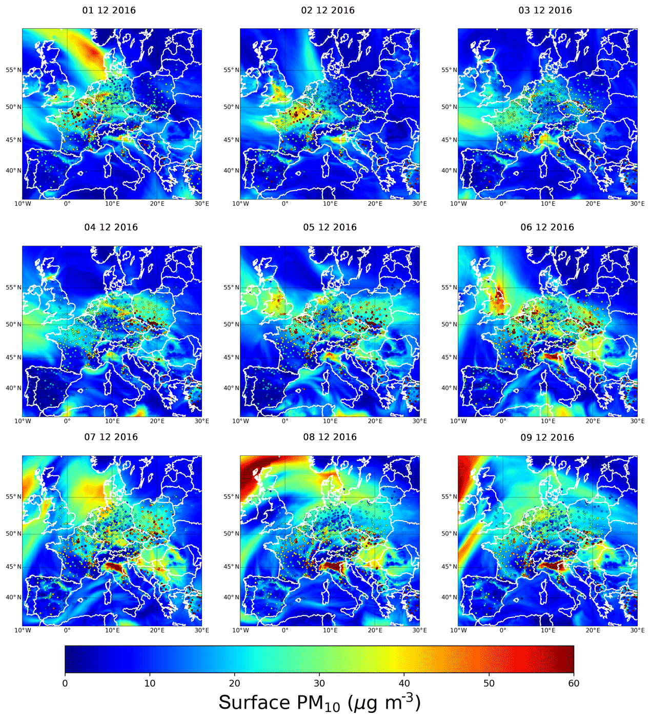
Figure 2Daily surface PM10 concentration, in micrograms per cubic metre, over Europe predicted by the EMEP model from 1 to 9 December 2016. The coloured dots correspond to the daily mean of AirBase stations (rural and urban stations).
During the following days relatively stable conditions with slow southerly winds characterized the episode until fronts moved in western Europe on 9 December. Large concentrations (> 60 µg m−3) were also predicted between 6 and 9 December over the Po Valley and over UK on 6 December (Figs. 2 and S2).
3.1 Statistical metrics used
To properly estimate the quality of these forecasts, five statistical parameters have been used, including the Pearson correlation (r), the mean bias (MB), the normalized mean bias (NMB), the root-mean-square error (RMSE), and the fractional gross error (FGE). The ideal score of these parameters is 0, except for the correlation, which is 1.
The MB provides information about the absolute bias of the model, with negative values indicating underestimation and positive values indicating overestimation by the model. The NMB represents the model bias relative to the reference. The RMSE considers error compensation due to opposite sign differences and encapsulates the average error produced by the model. The FGE is a measure of model error, ranging between 0 and 2, and behaves symmetrically with respect to under- and overestimation, without over emphasizing outliers.
We have used M and R as notation to refer, respectively, to model and the reference data (e.g. observations), and N is the size of the reference data set (e.g. number of observations).
Thus, MB is calculated by Eq. (1) and expressed in micrograms per cubic metre as follows:
NMB is calculated by Eq. (2):
RMSE is calculated by Eq. (3) and expressed in micrograms per cubic metre as follows:
and FGE is calculated by Eq. (4) and is dimensionless,
3.2 Comparison with observations
3.2.1 Methodology
In order to evaluate the reliability of the predictions over each city, the modelled hourly PM10 concentrations have been compared with the AirBase data (see https://www.eea.europa.eu/data-and-maps/data/airbase-the-european-air-quality-database-8#tab-data-by-country, last access: 27 March 2020). The traffic stations were not included in the comparison since a regional model with a somewhat-coarse resolution will not be able to calculate very large concentrations (e.g. hourly concentration higher than 200 µg m−3), which may be measured by these stations. Indeed, the concentrations calculated by a regional model over cities are mostly representative of the urban background. By knowing this point, we can state that a comparison with the observations presenting for example a correlation coefficient equal to 0.5 or NMB lower than 15 % is a reasonable result (r≥0.7 and NMB ≤ 10 % are good results). The observations have also been categorized into two sets of data by differentiating between the rural stations and the urban stations (as shown in Fig. S2). This follows the procedure done in the yearly evaluation of the EMEP model over Europe (e.g. EMEP Status Report, 2018). Due to the relatively coarse definition of a city, it appears that stations classified as rural may be present in our city domain.
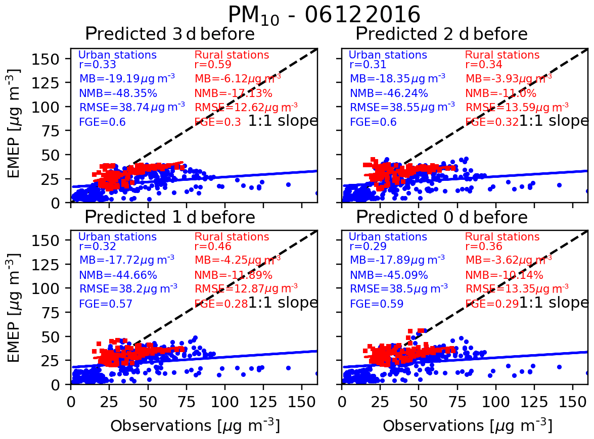
Figure 3Scatterplots between the hourly PM10 concentrations, in micrograms per cubic metre, over all of the studied cities using the nine grid cells definition, predicted by the EMEP model on 6 December 2016 and the observations of the urban sites (blue dot) and rural sites (red square). For this case, there are 19 cities which have urban stations in their domain and five cities which have rural stations in their domain. The observations are collocated in time with the EMEP predictions and then averaged within the city edge to match the studied grid. The four panels correspond to the different predictions from 3 d before the 6 December to the actual day, i.e. 6 December. The correlation coefficient (r), the mean bias (MB), the normalized mean bias (NMB), the root-mean-square error (RMSE), and the fractional gross error (FGE) are provided on each panel. The blue and the red lines represent the linear fits.
This was noticed for the smaller definition of the city edges, i.e. one grid cell there were no rural stations within the city domain. Obviously, by increasing the size of the city domain, to nine grid cells or by using the GADM definition, the number of rural stations present within the city domain increases. Indeed, all of the hourly measurements are averaged within the city boundary, by separating the urban and the rural stations. A comparison with these two types of stations can highlight a difference between the urban background and the urban concentrations. For such a comparison, the model concentrations are also averaged over the city domain.
3.2.2 Results
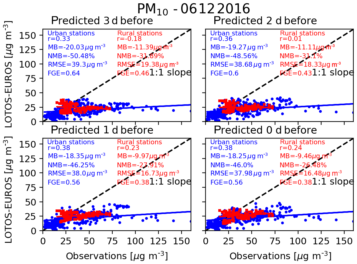
Figures 3 and 4 show the comparison between the hourly averaged observations within the city edges defined by the nine grid cells definition and the predictions from EMEP and from LOTOS-EUROS, respectively.
Figures 3 and 4 show that for the urban stations, the different predictions from the same model, for the same date, are consistent since the values for the statistical parameters are relatively constant. It is noticed, however, that the bias is slightly reduced when the starting date of the forecast is closer to the target date. The available observations and thus the stations may also differ from day to day (e.g. Fig. S2a). Figures 3 and 4 also show that despite many differences, the models have very similar performances in comparison with the urban stations.
In Fig. 3, it is also clear that the EMEP model has difficulties reproducing the highest concentrations measured by the urban stations, which are probably smoothed by the model over the large grid cells, as are the ones defining the cities. The underestimation of the largest urban concentrations is highlighted by the comparison with the rural stations. This also shows that over the area defining the cities there is a large variability in the measured PM10 concentrations and that few stations are not necessarily representative of the model grids. It also shows with such a resolution, the model represents urban background concentrations.
Only five cities have measurements defined as rural stations by using the nine grids definition (i.e. Amsterdam, Berlin, Luxembourg, Rotterdam, and Vienna) while there are up to 19 cities with urban stations. By comparing only the five cities having urban and rural stations, the agreement between EMEP and the urban stations is largely improved as shown in Fig. S3. We also notice that the difference in concentrations predicted by the EMEP model between both types of stations is also reduced. This shows that for these five cities, the predicted PM10 concentrations on 6 December are higher than over the other cities.
LOTOS-EUROS is less correlated with the concentrations measured by the rural stations than EMEP (Fig. 4). However, like EMEP, LOTOS-EUROS also presents a lower bias for these rural stations in comparison with the urban stations. This is predictable since with such a resolution, the model calculates mainly the urban background concentrations. By comparing the five cities having urban and rural stations, as done with EMEP, only the bias and the FGE between the predictions and the urban measurements are improved (Fig. S4). It is also worth noting that the concentrations predicted by LOTOS-EUROS over these five cities are lower than the ones calculated by the EMEP model (in Fig. S3).
By using the GADM definition, the number of cities having rural stations decreases to two, while the number of cities with the urban stations remains identical.
In general, both models present similar performances relative to the observations especially for the NMB, RMSE, and FGE as presented in Figs. S5 and S6. These figures show an overview of the statistical parameters for all 4 d forecasts, i.e. the dates from 1 to 12 December 2016 with a starting date from 1 to 9 December, for all of the cities defined by nine grid cells, in comparison with the concentrations measured at the urban and the rural stations, respectively.
As already shown by Figs. 3 and 4, LOTOS-EUROS shows slightly better correlation coefficients for the urban stations than EMEP (Fig. S5; on average RLOTOS-EUROS=0.31 and REMEP=0.25, with a maximum of 0.58 for LOTOS-EUROS and 0.5 for EMEP) and EMEP presents better correlations with the few rural stations (Fig. S6; on average RLOTOS-EUROS=0.23 and REMEP=0.35, with a maximum of 0.58 for LOTOS-EUROS and 0.72 for EMEP). However, the limited number of cities having rural stations explain the larger variability in the correlations compared to the correlations found with the urban stations. Similar results are found by using the GADM definition (not shown), while by using only one grid to define the city edges, the correlation coefficients with the urban stations are larger (up to 0.8), with an increase in the bias and a decrease in the RMSE (Fig. S7).
On average, both models have a FGE equal to 0.5 over the cities defined by nine grid cells with the urban stations and 0.4 with the rural stations. For the RMSE, it is 33 µg m−3 with the urban stations and 11 µg m−3 with the rural stations. While both models underestimate the PM10 concentrations by 36 % on average by using the urban sites, EMEP overestimates by 6 % with the rural stations, and LOTOS-EUROS underestimates this by 6 %.
Performances of both models are improved with daily means, especially with better correlation coefficients (not shown). For example, with the cities defined by nine grid cells, the correlation coefficients reach 0.8 with the urban stations for EMEP and LOTOS-EUROS and 0.98 with the rural stations for EMEP. However, a lot of negative correlation coefficients between LOTOS-EUROS and the rural stations are noticed. The correlation coefficient with the rural stations remains difficult to interpret, related to the limited number of stations available. Thus, EMEP presents a mean correlation coefficient equal to 0.4 for the urban and rural stations, and LOTOS-EUROS has a mean correlation of 0.5 with the urban stations and only 0.06 with the rural stations. Better scores with the FGE and the RMSE are also noticed in comparison to the hourly evaluation (not shown). Both models present, with the nine grid cells definition, a mean FGE of 0.5 with the urban stations and 0.3 for the rural stations and a mean RMSE of 21 µg m−3 with the urban stations and 10 µg m−3 with the rural stations.
3.3 Intercomparison in the concentrations predicted by both models
The second analysis has been focused on the agreement between both models. During the episode, all 4 d forecasts present a high correlation between the PM10 predicted by the EMEP model and LOTOS-EUROS as shown in Fig. 5a. These correlations vary from day to day and city by city but remain large for the different simulated periods (median = 0.7).
There is no clear geographical pattern in terms of performance between the two models, even if the central European cities (e.g. Budapest, Vienna, and Warsaw) presented the larger differences (Fig. 5b). These differences may be explained by not only by slightly lower secondary inorganic aerosols (SIA = ) in LOTOS-EUROS for these cities but also the lack of water in LOTOS-EUROS (which is not diagnosed as mentioned in Sect. 2). Moreover, it confirms the larger PM10 concentrations predicted by EMEP than by LOTOS-EUROS for the five cities plotted in Figs. S3 and S4. It is also worth noting that LOTOS-EUROS predicts more sea salt and dust for almost all of the cities during the studied period (Fig. S8), which is representative of the overall feature over the regional domain (not shown). Actually, it was noticed that for the predicted PM10 with the larger positive NMB (EMEP predicting larger PM10 concentrations), EMEP has more SIA and ”other” than LOTOS-EUROS (Fig. S9a), while the PM10 from LOTOS-EUROS is dominated by natural components when a larger negative NMB is predicted (Fig. S9b).
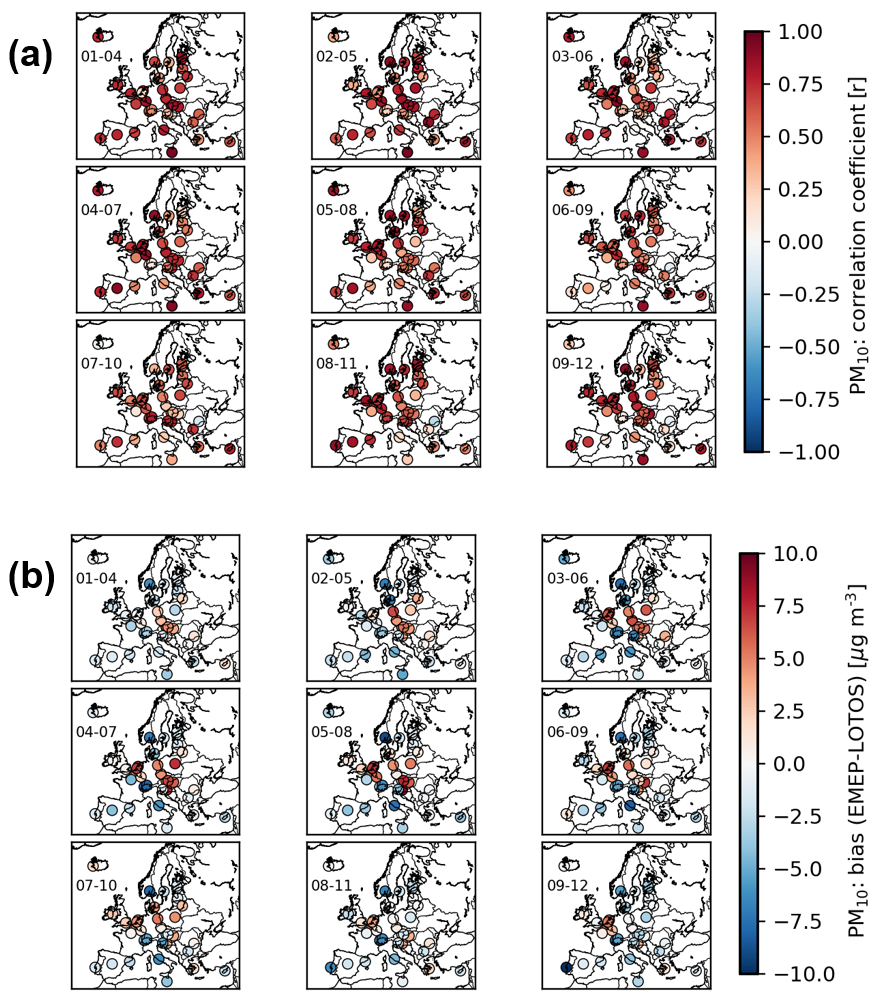
Figure 5(a) Correlation coefficient and (b) bias in the predicted PM10 concentrations between the EMEP model and LOTOS-EUROS over all of the studied cities using the nine grid cells definition for each 4 d forecast (1–4, 2–5, 3–6, 4–7, 5–8, 6–9, 7–10, 8–11, and 9–12 December 2016).
4.1 The EMEP model
4.1.1 Emission reductions
The SC calculation follows the methodology used in each EMEP annual report to quantify the annual country-to-country source–receptor relationships (e.g. EMEP Status Report, 2018). The experiment is based on a reference run, where all of the anthropogenic emissions are included. The other runs are the perturbation runs. These runs correspond to the simulations where the emissions from every considered country are reduced by 15 %. As explained in Wind et al. (2004), a reduction of 15 % is sufficient to give a clear signal in the pollution changes. It also causes a negligible effect from nonlinearity in the chemistry even if in this work it has been estimated.
The perturbation runs are done for anthropogenic emissions of CO, SOx, NOx, NH3, non-methane volatile organic compounds (NMVOCs), and PPM (primary particulate matter). For computational efficiency, in the perturbation calculations, all anthropogenic emissions in the perturbation runs have been reduced here simultaneously. This simultaneous reduction differs from the methodology used in each EMEP annual report where the emissions are reduced individually.
There are in total 31 runs for each date with reduced anthropogenic emissions. Each run corresponds to the perturbations for one of the 28 countries related to the 28 EU capitals, plus Iceland, Norway and Switzerland, giving the contribution for each country.
To calculate the concentration of the pollutant integrated over the studied area, i.e. a selected city, coming from a source, we follow the Eq. (5):
where x is the reduction in percent (i.e. 0.15), Creference is the concentration of the pollutant integrated over the studied area from the reference run, and Cperturbation is the concentration of the pollutant integrated over the studied area from the perturbation run. Thus, by differentiating over the studied area, the concentration from the perturbed run with the concentration provided by the reference run, we have an estimation of the influence of the source (i.e. country). By scaling with the reduction used (parameter x), it gives the estimated concentration related to the source.
4.1.2 Issue concerning the chemical nonlinearity
The reason why emissions should not be perturbed by 100 % in the model simulations is to stay within the linear regime of involved chemistry. Even limited, such a methodology may still introduce a nonlinearity in the chemistry. The total PM10 over the receptor should be identical theoretically to the sum of the PM10 originated from the different sources. This is not always the case, and the difference between the total PM10 and the sum from the various sources may lead to negative or positive concentrations. This is a result of the perturbation used, which is assumed to be linear for a 100 % perturbation.
The 15 % emission reduction has been used for many years for the annual country-to-country source–receptor relationships calculations (e.g. EMEP Status Report, 2018). Clappier et al. (2017a) have already shown the robustness of the methodology at the country scale on yearly averages and for the highest daily concentrations. However, this emission reduction was not used for smaller areas. Thus this 15 % emission reduction for the study over a city and on hourly basis has been tested, in order to assess the robustness of the calculations. The values 5 % and 50 % were the other selected emission reductions. In total, 847 4 d runs have been performed in this work (nine reference runs and nine dates × 31 countries × 3 perturbations runs).
Furthermore, by reducing the emissions simultaneously or separately may lead to a different result in the concentrations, but as mentioned previously, this effect is not addressed in this work for computational reasons.
4.2 LOTOS-EUROS
A labelling technique has been developed within each LOTOS-EUROS simulation (Kranenburg et al., 2013). An important advantage of the labelling technique is the reduction in computation costs and analysis work associated with the calculations. The source apportionment technique has been previously used to investigate the origin of PM (Hendriks et al., 2013, 2016), NO2 (Schaap et al., 2013), and nitrogen deposition (Schaap et al., 2018).
Besides the concentrations of all species, the contributions of a number of sources to all components are calculated. The labelling routine is only implemented for primary, inert aerosol tracers and chemically active tracers containing a C, N (reduced and oxidized), or S atom, as these are conserved and traceable. This technique is therefore not suitable to investigate the origin of e.g. O3 and H2O2, as they do not contain a traceable atom. The source apportionment module for LOTOS-EUROS provides a source attribution valid for current atmospheric conditions as all chemical conversions occur under the same oxidant levels. For details and validation of this source apportionment module we refer to Kranenburg et al. (2013).
To avoid violating the memory size and to avoid excessive computation times it was chosen to trace the 28 EU countries, supplemented by Norway and Switzerland. For convenience, a number of small countries were combined with a neighbouring country. For example, Switzerland and Liechtenstein and Luxembourg and Belgium were combined. In addition, all sea areas were combined into one source area. To be mass consistent, all non-specified regions, natural emissions, and the combined impact of initial conditions and boundary conditions were given labels as well.

Figure 6Mean composition of (a) Domestic, (b) 30 European countries, and (c) Others PM10, split into a negative concentration (left panel) and a positive concentration (right panel), calculated by the EMEP country SC over the 34 European cities and for each 4 d forecast. The PM10 composition is highlighted with the colour code. The results for the three city definitions (one grid, nine grids, and GADM) and for the percentage of reduction used in the perturbation EMEP runs (5 %, 15 %, and 50 %) are shown. The Domestic contribution corresponds to the contribution from the domestic country to the city (e.g. from France to Paris). The label 30 European countries corresponds to the other 30 European countries used in the study. Others contains natural sources, the other countries included in the regional domain, boundary conditions, ship traffic, biogenic sources, aircraft emissions, and lightning. The red dot represents the mean PM10 concentration.
5.1 In the EMEP calculations
As presented in Fig. 1, the country contributions to the predicted PM10 concentrations in the cities is provided in our products.
Figure 6 presents the mean composition for the “Domestic”, “30 European” countries, and “Others” PM10 contributions for all cities, for all 4 d predictions, and split into negative and positive concentrations. This figure is a result of the perturbation runs by separating the positive and the negative concentrations obtained in the calculations. The concentrations have also been gathered by their calculated origin. The Domestic contribution corresponds to the contribution from the domestic country to the city (for example from France to Paris). The 30 European countries corresponds to the other 30 European countries used in the study. Others contains mainly natural sources, the other European countries included in the regional domain (and not included in our SC calculations, e.g. Turkey), and the boundary conditions. This figure gives a graphical illustration of the composition of the different contributions and presents the effect of the nonlinearity. Indeed, the positive concentrations show the overall composition for each contribution, while the chemical reason of the nonlinearity is highlighted by the negative contribution to the predicted PM10 concentrations.
The main contributors to the Domestic PM10 are POM (∼ 20 %) and rest PPM (∼ 30 %) (which corresponds to the remainder of coarse and fine PPM), as noticed for the positive concentrations (Fig. 6a). Actually, the variation in the mean concentrations is mainly influenced by the variation in these primary components. is also an important component of the Domestic PM10. The value of the mean concentration depends on the city definition ,and so on the average of the concentrations over different size of city. The mean PM10 concentration over a smaller area is larger, showing that with a smaller grid, the PM10 is less diffused over the integrated area. The 30 European countries PM10 is mainly influenced by (by 38 %) (Fig. 6b).
Overall, 45 % of the contributions to the PM10 calculated over the selected cities for this episode are Domestic and essentially due to primary components. 35 % are from the 30 European countries, essentially , and 25 % are from Others, mainly composed of natural sources (representing 50 % of Others). Obviously, this feature is an overview of all selected cities for all of the studied dates and it can vary from city to city and from date to date.
By comparing the PM10 concentrations calculated over the same city edges but by using different percentages in the perturbation runs, we have calculated the impact of the nonlinearity for each contribution and presented this in Fig. 7. This nonlinearity has been calculated for each hourly concentration as the standard deviation of the hourly contribution (which can be positive or negative) obtained by the three reduced emissions scenarios and weighted by the hourly total concentration by following the Eq. (6):
where n corresponds to the number of perturbations used (n=3), Ccontrib is the hourly PM10 concentration for a specific contribution (Domestic, 30 European countries, or Others), and Ctot is the hourly PM10 concentration. This mean nonlinearity due to the Domestic contribution represents a maximum of 0.9 % of the total PM10. This nonlinearity from the 30 European countries contribution counts for 0.7 % of the total PM10 and 1.5 % from Others. Actually, the nonlinearity from the Others depends on the nonlinearity from the two other contributions. The mean nonlinearity is not homogenously distributed over all cities as shown in Fig. S10 and may vary from date to date (not shown). It has remained limited even if some hourly contributions show higher nonlinearity. At the maximum, 3 % of the calculated hourly contributions for all 4 d forecasts over the selected cities have a nonlinearity higher than 5 % (not shown). This shows that due to the methodology used in the EMEP model, based on a reduced emission scenario, the nonlinearity in the chemistry has a limited impact on the SC calculation. This nonlinearity is slightly reduced by using the larger domains to define the cities (e.g. nine grids) (Fig. 7). This also shows that the responses to perturbation runs are robust, even if only the nonlinearity in the chemistry related to the perturbation used and not the one related to the reduction in each emission precursor has been estimated in this study as mentioned in Sect. 4.1.
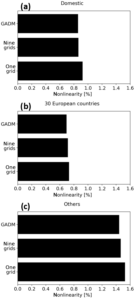
Figure 7The black horizontal bars show the mean nonlinearity calculated for each contribution presented in Fig. 6 and for the three city definitions. The nonlinearity is calculated for each hourly concentration as the standard deviation of the hourly contribution weighted by the hourly total concentration.
Negligible negative contributions have been calculated for the Domestic and 30 European countries contributions (Fig. 6a and b), and small negative contributions are predicted in Others (Fig. 6c). These negative PM10 are a result of negative values in , , and H2O, which are a consequence of gas–aerosol partitioning of the species. Indeed, NH3 reacts with nitric acid (HNO3) to form ammonium nitrate (NH4NO3). This is an equilibrium reaction and thus the transition from solid to gaseous phase depends on relative humidity (e.g. Fagerli and Ass, 2008; Pakkanen, 1996). This shows that, for example, a reduction in NOx over a country, which impacts the selected city, does not necessarily only impact the over this city but may also have an effect on NH3 chemistry over a second region. This second region may also have itself an impact on the selected city. This combination of NOx and NH3 chemistry from different regions may lead at the end to these negative concentrations.
The impacts of the percentage used in the perturbation runs and the size of the city edges have no significant impact on the amount of negative Others PM10 concentrations. The impact of both parameters is more visible on the Domestic and 30 European countries concentrations but it remains very small.
Averaging out over the larger grids reduces globally the nonlinearity. The 15 % emission reduction also reduces the negative nonlinearity in the Domestic concentrations (e.g. H2O for the nine-grid and GADM runs).
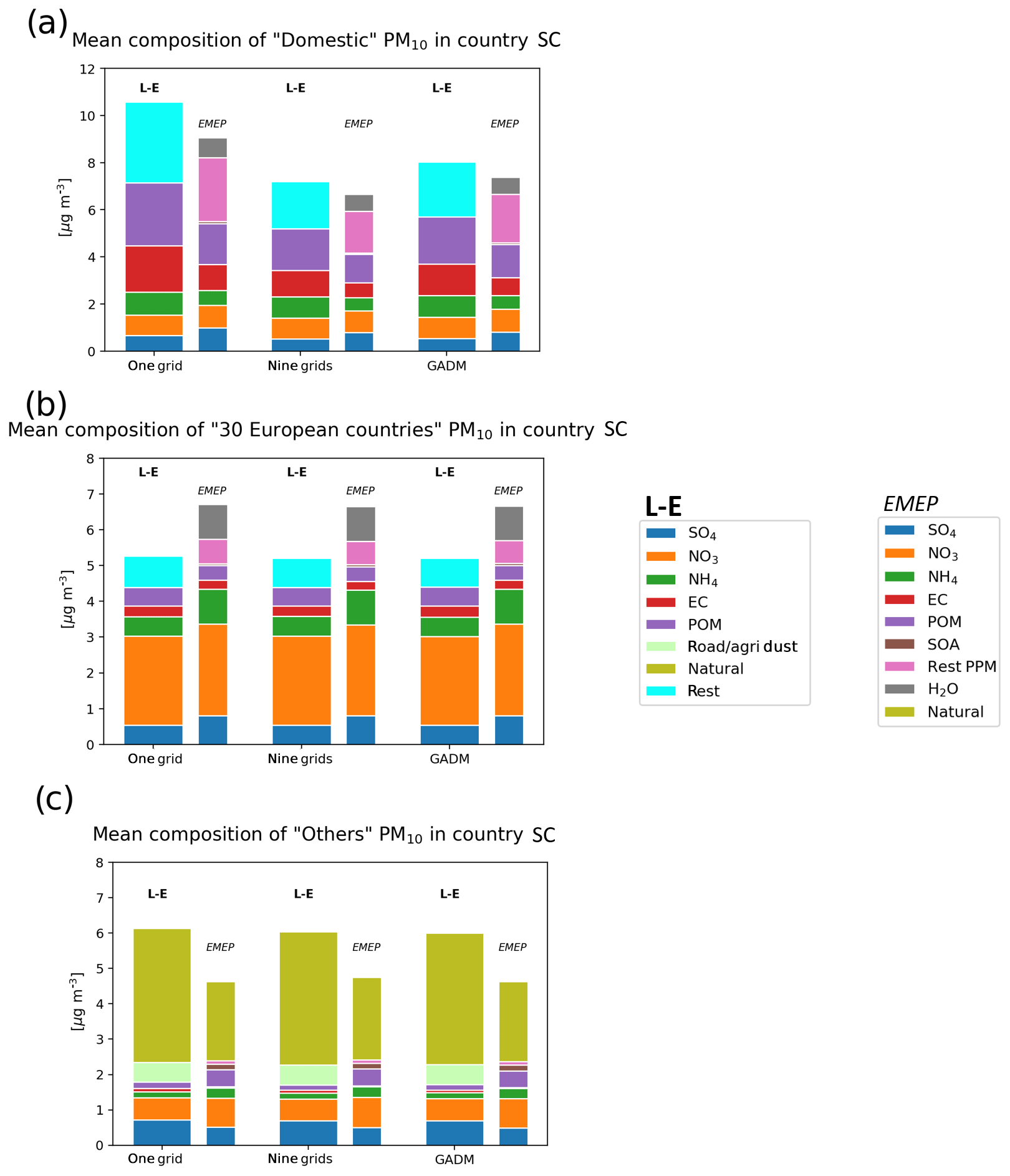
Figure 8Mean composition of (a) Domestic, 30 (b) European countries, and (c) Others PM10 calculated by the LOTOS-EUROS (L-E) country SC over the 34 European cities and for each 4 d forecast. The result from the EMEP country SC, by using a 15 % perturbation run, has also been added for comparison. The PM10 composition is highlighted with the colour code. Rest corresponds to the difference between the PM10 and the sum of the components listed on the plot. The results for the three city definitions (one grid, nine grids, and GADM) are shown. The Domestic contribution corresponds to the contribution from the domestic country to the city (e.g. from France to Paris). The label 30 European countries corresponds to the other 30 European countries used in the study. Others in the LOTOS-EUROS country SC is slightly different from the EMEP Others. Others in the LOTOS-EUROS country SC contains natural sources, other countries included in the regional domain, boundary conditions, dust emitted by road traffic and agriculture, ship traffic, the aircraft emissions, and lightning.
5.2 In the LOTOS-EUROS calculations
As presented with the EMEP predictions, Figure 8 presents the mean composition for the Domestic, 30 European countries, and Others PM10 contributions for all cities, for all 4 d predictions provided by LOTOS-EUROS. The definition of Others is slightly different from the EMEP one since, for example, the dust from agriculture and traffic is included (see Sect. 2). For an easier comparison, the result for the EMEP model using the 15 % emission reduction has also been plotted with thinner charts, even if, as just mentioned, the definition of Others slightly differs between both models.
First of all, during the episode, LOTOS-EUROS confirms the general trend calculated by the EMEP model, i.e. the dominant contribution to the surface PM10 is Domestic, ranging between 40 % and 48 % of the predicted PM10 over all selected cities and for all of the studied dates. However, LOTOS-EUROS always presents more Domestic PM10 than the EMEP model. LOTOS-EUROS also predicted slightly more influence from Others than the 30 European countries, with ratios close to 25 %–30 % each. As a reminder, the EMEP model predicted a slightly larger influence from the 30 European countries (35 %) than from Others (25 %).
As with the EMEP model, the mean PM10 concentration over the smaller city definition is larger, and the Domestic PM10 is largely driven by POM. In the list of LOTOS-EUROS PM10 components there is one named “Rest”. Rest corresponds to the difference between the total PM10 and the sum of all of the components, and Fig. 8 shows that it is also a large component of this Domestic PM10. POM and Rest each represent between 25 % and 30 % of the Domestic PM10.
The large influence of (48 %) on the 30 European countries PM10 is also calculated by LOTOS-EUROS, as well as the large contribution of the natural components (60 %) in Others. It is noteworthy to see that, even being small, the dust emitted by the road traffic and the agriculture is not negligible in Others PM10 (∼ 10 %).
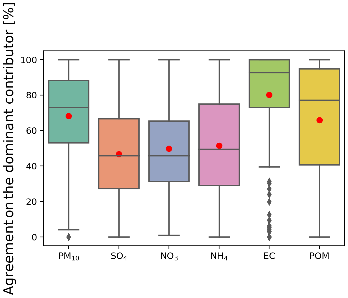
Figure 9Agreement on the determination of the dominant country contributor for PM10, SO4, NO3, NH4, EC, and POM in percent, determined over all of the studied cities using the nine grid cells definition and for all 4 d forecasts. The line that divides the box into two parts represents the median of the data. The ends of the box show the upper and lower quartiles. The extreme lines show the highest and lowest values excluding outliers, which are represented by grey diamonds. The red dots correspond to the mean of each data set.
Section 3 has highlighted the similar performance of both models in the prediction of the PM10 concentrations over the European cities with observations. It has also been shown in Sect. 3 that both models are representative for a large area, and the predictions can underestimate the concentrations and the contributions for the larger concentrations measured by a specific station. Section 5 has shown similar results in terms of composition of these PM10. It is also noteworthy to see in Fig. 9 that both SC calculations present a high rate of agreement over the selected period with the common simulated components and the PM10 calculated by both models. This rate corresponds to the number of occurrences in the dominant contributor calculated for each hourly concentration in the 4 d forecast over each city. So, a value of 100 % over a city shows that both models predict the same dominant country contributor during a 4 d forecast. In Fig. 9, both models show that, by using the nine grid cells definition, on average 68 % of the hourly predicted PM10 concentrations have the same dominant country contributor. On average, 50 % of the secondary inorganic aerosols predicted by both models over all of the cities and all 4 d forecasts have the same main contributor. This value goes up to 70 % for POM and 80 % for EC. For the two primary components (POM and EC) the median is larger, with values of 77 % and 93 %, respectively, showing that the mean value in the agreement for both compounds is reduced by a few low values (Fig. 9). On a daily basis, the mean agreement is slightly improved, e.g. 70 % agreement for the PM10 (Fig. S11). The main improvement is calculated for EC, with a median equal to 100 % (Fig. S11).
The lower agreement for the SIA is predictable due to the various origins (chemistry and primary emissions) for these particulates and the different aerosols treatment (gas–aerosol partitioning) in both models. It is also related to the differences in both methodologies (e.g. Clappier et al., 2017b). Indeed, an emission reduction and a labelling technique will not necessarily provide the same results for the secondary PM. An emission reduction depends on the atmospheric composition already present. For example, an amount of NOx emitted over a source can result in a certain NH4NO3 concentration in the receptor. If this NOx is emitted in excess (NH3-limited regime), a NOx emission reduction will have a small effect at the receptor point. On the other hand, in the NOx-limited regime, the same NOx reduction will have a large impact. The labelling method will give the same result in both cases, while the scenario approach will give different results.
This agreement varies from city to city (Fig. 10), but it has been shown, in addition to the example of PM10 (Fig. 5), that central European cities often present a limited agreement due to their central location and the influence of various countries. This limited agreement is also sometimes observable for the cities close to the edge of the regional domain (Fig. 10), which could be explained by the influence of the boundary conditions such as the dust transported from other regions (e.g. Valetta influenced by dust from Sahara).
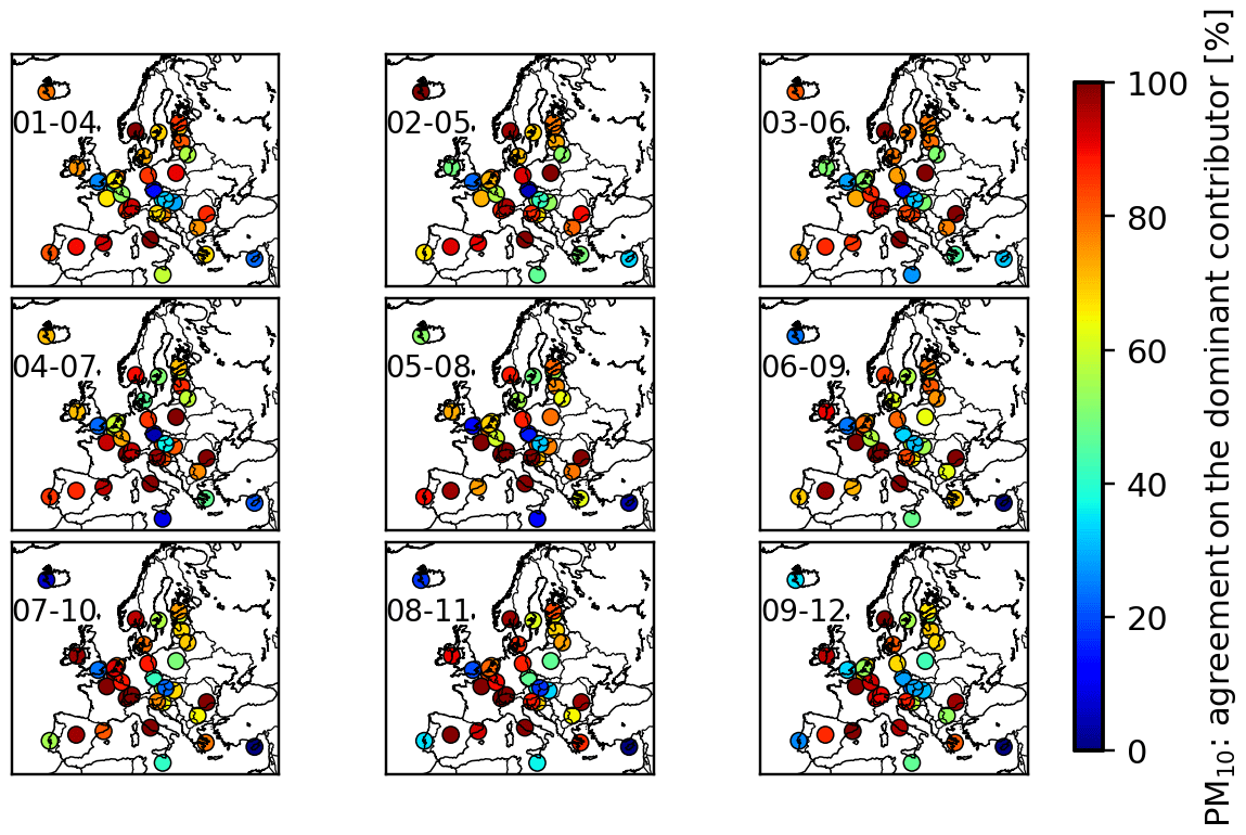
Figure 10Agreement on the determination of the dominant country contributor for PM10 in percent, and for each 4 d forecast (1–4, 2–5, 3–6, 4–7, 5–8, 6–9, 7–10, 8–11, and 9–12 December 2016) over all of the cities using the nine grid cells definition.
The mean agreement increases to up to 75 % for the determination of the top five main country contributors to PM10 (Fig. 11). In that case, the rate is calculated for the five main country contributors. A score of 100 % means both models predict the same five main country contributors for each hourly concentration but not necessarily in the same order. This rate is around 70 % for , EC, and POM, close to 60 % for , and equal to 65 % for (Fig. 11). As for the dominant country contributor, the agreement is slightly improved by using daily means; e.g. we found 76 % agreement with the PM10 (not shown).
It is also important to notice that these overall agreements are significantly influenced by neither the definition of the area of the cities nor the perturbation percentage tested for the EMEP SC calculations (Fig. S12). The agreement becomes slightly better by using the smaller area (1 grid) in the determination of the dominant country contributor and by using a large domain (nine grids or GADM) in the determination of the two and five main contributors.
Overall, a perturbation run using a reduction of 15 % and the use of a larger city area (e.g. GADM or nine grids) allow a better determination of the country contributors, with a better agreement with LOTOS-EUROS, and limit the impact of the nonlinearity in the chemistry.
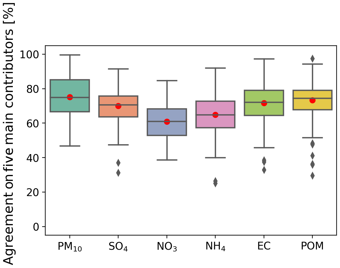
Figure 11Agreement on the determination of the five main country contributors for PM10, SO4, NO3, NH4, EC, and POM in percent, determined over all of the studied cities using the nine grid cells definition and for all 4 d forecasts. The line that divides the box into two parts represents the median of the data. The ends of the box show the upper and lower quartiles. The extreme lines show the highest and lowest values excluding outliers, which are represented by grey diamonds. The red dots correspond to the mean of each data set.
By focusing on a specific event, occurring from 1 to 9 December 2016 over Europe, this work is the first attempt to evaluate the source contribution calculations provided by two regional models (EMEP and LOTOS-EUROS) in a forecast mode. Together, the models compose the operational source contribution prediction system for the European cities within the Copernicus Atmosphere Monitoring Service (CAMS) and aim to estimate the impact of the long-range transport to urban PM10. These models also use two distinct source apportionment methodologies, a labelling technique for LOTOS-EUROS and the use of perturbation runs for EMEP.
The methodology used for the EMEP model was tested by using three different percentages (5 %, 15 %, and 50 %) in the perturbation runs. The importance of the choice of the domain-defining the edges of the studied cities was also investigated in terms of predicted concentrations and calculated contributors. It was concluded that the 15 % emission reduction and the use of large city areas (nine grids or GADM) were the more efficient. It reduces the impact of nonlinearity, which especially impacts the , , and H2O concentrations, and it presents a better agreement on the determination of the main country contributors. The mean nonlinearity always represents less than 2 % of the total modelled PM10 for each contribution calculated by the EMEP SC and is caused by the perturbation used, which is assumed to be linear for a 100 % perturbation. Even if this nonlinearity is not identical for all cities and for the different dates, the larger nonlinearities (> 5 %) impact only 3 % of all of the calculated hourly contributions. However, the nonlinearity related to the reduction in each emission precursor has not been calculated in the study for computational reasons.
The predicted PM10 concentrations were compared with AirBase observations, showing fair agreement even if the models remain perfectible since they have difficulties reproducing the highest hourly concentrations measured by the urban stations (mean underestimation of 36 %). It may suggest that both models, which calculate the country contributions over the cities, defined by a large area, may underestimate the contribution measured by a specific station for the higher concentrations. It was also noticed that the bias is slightly reduced when the forecast is closer to the studied date. An intercomparison between both models was also performed showing satisfactory results with few discrepancies in the predictions of the PM10 concentrations, mainly explained by an underestimation of sea salt and dust by the EMEP model (compared to LOTOS-EUROS) and differences in SIA, caused by different chemical aerosols treatment in both models.
During the episode, both models have shown that 45 % of the predicted PM10 over the selected cities were from Domestic sources and essentially composed of primary components. The rest of the contribution was roughly equitably split into an influence from the other 30 European countries used in the regional domain, essentially composed of , and an influence from Others, mainly composed of natural sources.
We have shown that results from both source apportionment methodologies agree on average by 68 % in the determination of the dominant country contributor to the hourly PM10 concentrations and by 75 % for the top five of these country contributors. Calculating the country attribution on a daily-mean basis has similar agreement. Where there are differences, these are mainly found in the country attribution of the secondary inorganic component of the aerosol. These differences derive from a combination of the different treatment of these secondary components and the different method used to attribute country contributions between the models being compared.
A full year of evaluation will be necessary to confirm our satisfactory results. Moreover, the bias of the predicted PM10 concentrations for the urban observations probably suggests an underestimation of the local background contribution (from the city), which is also predicted by the EMEP model. This is investigated in a companion paper (Pommier et al., 2020), also focusing on the same event.
The EMEP model is an open-source model available on https://doi.org/10.5281/zenodo.3355041 (EMEP MSC-W, 2017). The base code of LOTOS-EUROS is available under the license on https://lotos-euros.tno.nl/ (last access: 27 March 2020), but the code used for this study, including the source apportionment, is only available in cooperation with TNO. The data processing and analysis scripts are available upon request.
The supplement related to this article is available online at: https://doi.org/10.5194/gmd-13-1787-2020-supplement.
MP, HF, and MiS designed the research. MP performed the experiment. MP developed the analysing codes and analysed the data. AV developed the EMEP part of the forecasting system. RK and MaS performed and provided the LOTOS-EUROS results. MP wrote the paper with the inputs from all coauthors.
The authors declare that they have no conflict of interest.
This work is partly funded by the EU Copernicus project CAMS 71 to provide policy support. This work has also received support from the Research Council of Norway (Programme for Supercomputing) through the EMEP project (NN2890K) for CPU and the NorStore project “European Monitoring and Evaluation Programme” (NS9005K) for storage. The EMEP project itself is supported by the Convention on Long-range Transboundary Air Pollution (LRTAP), under UNECE. The authors thank A. Mortier (Norwegian Meteorological Institute) for the development and the design of the website (https://policy.atmosphere.copernicus.eu/SourceContribution.php, last access: 27 March 2020).
This research has been supported by the Research Council of Norway (grant no. NN2890K) and the NorStore project “European Monitoring and Evaluation Programme” (grant no. NS9005K).
This paper was edited by Graham Mann and reviewed by Richard Pope and one anonymous referee.
Amann, M., Bertok, I., Borken-Kleefeld, J., Cofala, J., Heyes, C., Höglund-Isaksson, L., Klimont, Z., Nguyen, B., Posch, M., Rafaj, P., Sandler, R., Schöpp, W., Wagner, F., and Winiwarter, W.: Cost-effective Control of Air Quality and Greenhouse Gases in Europe: Modeling and Policy Applications, Environ. Model. Softw., 26 ,1489–1501, 2011.
Andersson-Sköld, Y. and Simpson, D.: Comparison of the chemical schemes of the EMEP MSC-W and the IVL photochemical trajectory models, Atmos. Environ., 33, 1111–1129, https://doi.org/10.1016/S1352-2310(98)00296-9, 1999.
Banzhaf, S., Schaap, M., Kerschbaumer, A., Reimer, E., Stern, R., van der Swaluw, E., and Builtjes, P.: Implementation and evaluation of pH-dependent cloud chemistry and wet deposition in the chemical transport model REM-Calgrid. Atmos. Environ., 49, 378–390, https://doi.org/10.1016/j.atmosenv.2011.10.069, 2012.
Bergström, R., Denier van der Gon, H. A. C., Prévôt, A. S. H., Yttri, K. E., and Simpson, D.: Modelling of organic aerosols over Europe (2002–2007) using a volatility basis set (VBS) framework: application of different assumptions regarding the formation of secondary organic aerosol, Atmos. Chem. Phys., 12, 8499–8527, https://doi.org/10.5194/acp-12-8499-2012, 2012.
Binkowski, F. S. and Shankar, U.: The Regional Particulate Matter Model 1. Model description and preliminary results, J. Geophys.Res., 100, 26191–26209, https://doi.org/10.1029/95JD02093, 1995.
Bott, A.: A positive definite advection scheme obtained by nonlinear renormalization of the advective fluxes, Mon. Weather Rev., 117, 1006–1016, https://doi.org/10.1175/1520-0493(1989)117(1006:APDASO)2.0.CO;2, 1989.
Brasseur, G. P., Xie, Y., Petersen, A. K., Bouarar, I., Flemming, J., Gauss, M., Jiang, F., Kouznetsov, R., Kranenburg, R., Mijling, B., Peuch, V.-H., Pommier, M., Segers, A., Sofiev, M., Timmermans, R., van der A, R., Walters, S., Xu, J., and Zhou, G.: Ensemble forecasts of air quality in eastern China – Part 1: Model description and implementation of the MarcoPolo–Panda prediction system, version 1, Geosci. Model Dev., 12, 33–67, https://doi.org/10.5194/gmd-12-33-2019, 2019.
Burr, M. J. and Zhang, Y.: Source apportionment of fine particulate matter over the Eastern U.S. – Part II: source sensitivity simulations using CAMX/PSAT and comparisons with CMAQ source sensitivity simulations, Atmosp. Pollut. Res., 2, 318–336, 2011.
Callaghan, A., de Leeuw, G., Cohen, L., and O'Dowd, C. D.: Relationship of oceanic whitecap coverage to wind speed and wind history, Geophys. Res. Lett., 35, L23609, https://doi.org/10.1029/2008GL036165, 2008.
Clappier, A., Fagerli, H., and Thunis, P.: Screening of the EMEP source receptor relationships: application to five European countries, Air Qual. Atmos. Health, 10, 497–507, https://doi.org/10.1007/s11869-016-0443-y, 2017a.
Clappier, A., Belis, C. A., Pernigotti, D., and Thunis, P.: Source apportionment and sensitivity analysis: two methodologies with two different purposes, Geosci. Model Dev., 10, 4245–4256, https://doi.org/10.5194/gmd-10-4245-2017, 2017b.
Crippa, M., Janssens-Maenhout, G., Dentener, F., Guizzardi, D., Sindelarova, K., Muntean, M., Van Dingenen, R., and Granier, C.: Forty years of improvements in European air quality: regional policy-industry interactions with global impacts, Atmos. Chem. Phys., 16, 3825–3841, https://doi.org/10.5194/acp-16-3825-2016, 2016.
Dockery, D. W. and Pope III, C. A.: Acute respiratory effects of particulate air pollution, Ann. Rev. Public Health, 15, 107–132, https://doi.org/10.1146/annurev.pu.15.050194.000543, 1994.
D'Elia, I., Bencardino, M., Ciancarella, L., Contaldi, M., and Vialetto, G.: Technical and Non-Technical Measures for air pollution emission reduction: The integrated assessment of the regional Air Quality Management Plans through the Italian national model, Atmos. Environ., 43, 6182–6189, https://doi.org/10.1016/j.atmosenv.2009.09.003, 2009.
EEA: Air quality in Europe 2017, EEA Report No 13/2017, available at: https://www.eea.europa.eu/publications/air-quality-in-europe-2017 (last access: 27 March 2020), 2017.
EMEP: Transboundary acidification and eutrophication and ground level ozone in Europe: Unified EMEP model description, EMEP Status Report 1/2003, The Norwegian Meteorological Institute, Oslo, Norway, ISSN 0806-4520, 2003.
EMEP: Transboundary particulate matter, photo-oxidants, acidifying and eutrophying components, EMEP Status Report 1/2018:, Joint MSC-W & CCC & CEIP Report, ISSN 1504-6109, 2018.
EMEP MSC-W: metno/emep-ctm: OpenSource rv4.15 (201709) (Version rv4_15), Zenodo, https://doi.org/10.5281/zenodo.3355041, 2017.
Fagerli, H. and Aas, W.: Trends of nitrogen in air and precipitation: Model results and observations at EMEP sites in Europe, 1980–2003, Environ. Poll., 154, 448–461, https://doi.org/10.1016/j.envpol.2008.01.024, 2008.
Founda, D., Kazadzis, S., Mihalopoulos, N., Gerasopoulos, E., Lianou, M., and Raptis, P. I.: Long-term visibility variation in Athens (1931–2013): a proxy for local and regional atmospheric aerosol loads, Atmos. Chem. Phys., 16, 11219–11236, https://doi.org/10.5194/acp-16-11219-2016, 2016.
Fountoukis, C. and Nenes, A.: ISORROPIA II: a computationally efficient thermodynamic equilibrium model for aerosols, Atmos. Chem. Phys., 7, 4639–4659, https://doi.org/10.5194/acp-7-4639-2007, 2007.
Gerber, H. E.: Relative-Humidity Parameterization of the Navy Aerosol Model (NAM), Naval Research Laboratory, NRL report 8956, 1985.
Grewe, V., Tsati, E., and Hoor, P.: On the attribution of contributions of atmospheric trace gases to emissions in atmospheric model applications, Geosci. Model Dev., 3, 487–499, https://doi.org/10.5194/gmd-3-487-2010, 2010.
Hendriks, C., Kranenburg, R., Kuenen, J., van Gijlswijk, R., Wichink Kruit, R., Segers, A., Denier van der Gon, H., and Schaap, M.: The origin of ambient particulate matter concentrations in the Netherlands, Atmos. Environ., 69, 289–303, https://doi.org/10.1016/j.atmosenv.2012.12.017, 2013.
Hendriks, C., Kranenburg, R., Kuenen, J.J.P., Van den Bril, B., Verguts, V., and Schaap, M.: Ammonia emission time profiles based on manure transport data improve ammonia modelling across north western Europe, Atmos. Environ., 131, 83–96, https://doi.org/10.1016/j.atmosenv.2016.01.043, 2016.
Jonson, J. E., Stohl, A., Fiore, A. M., Hess, P., Szopa, S., Wild, O., Zeng, G., Dentener, F. J., Lupu, A., Schultz, M. G., Duncan, B. N., Sudo, K., Wind, P., Schulz, M., Marmer, E., Cuvelier, C., Keating, T., Zuber, A., Valdebenito, A., Dorokhov, V., De Backer, H., Davies, J., Chen, G. H., Johnson, B., Tarasick, D. W., Stübi, R., Newchurch, M. J., von der Gathen, P., Steinbrecht, W., and Claude, H.: A multi-model analysis of vertical ozone profiles, Atmos. Chem. Phys., 10, 5759–5783, https://doi.org/10.5194/acp-10-5759-2010, 2010.
Kaiser, J. W., Heil, A., Andreae, M. O., Benedetti, A., Chubarova, N., Jones, L., Morcrette, J.-J., Razinger, M., Schultz, M. G., Suttie, M., and van der Werf, G. R.: Biomass burning emissions estimated with a global fire assimilation system based on observed fire radiative power, Biogeosciences, 9, 527–554, https://doi.org/10.5194/bg-9-527-2012, 2012.
Keuken, M, Zandveld, P., van den Elshout, S., Janssen, N. A. H., and Hoek, G.: Air quality and health impact of PM10 and EC in the city of Rotterdam, the Netherlands in 1985–2008, Atmos Environ., 45, 5294–5301, https://doi.org/10.1016/j.atmosenv.2011.06.058, 2011.
Kiesewetter, G., Borken-Kleefeld, J., Schöpp, W., Heyes, C., Thunis, P., Bessagnet, B., Terrenoire, E., Fagerli, H., Nyiri, A., and Amann, M.: Modelling street level PM10 concentrations across Europe: source apportionment and possible futures, Atmos. Chem. Phys., 15, 1539–1553, https://doi.org/10.5194/acp-15-1539-2015, 2015.
Kranenburg, R., Segers, A. J., Hendriks, C., and Schaap, M.: Source apportionment using LOTOS-EUROS: module description and evaluation, Geosci. Model Dev., 6, 721–733, https://doi.org/10.5194/gmd-6-721-2013, 2013.
Kuenen, J. J. P., Visschedijk, A. J. H., Jozwicka, M., and Denier van der Gon, H. A. C.: TNO-MACC_II emission inventory; a multi-year (2003–2009) consistent high-resolution European emission inventory for air quality modelling, Atmos. Chem. Phys., 14, 10963–10976, https://doi.org/10.5194/acp-14-10963-2014, 2014.
Manders, A. M. M., Builtjes, P. J. H., Curier, L., Denier van der Gon, H. A. C., Hendriks, C., Jonkers, S., Kranenburg, R., Kuenen, J. J. P., Segers, A. J., Timmermans, R. M. A., Visschedijk, A. J. H., Wichink Kruit, R. J., van Pul, W. A. J., Sauter, F. J., van der Swaluw, E., Swart, D. P. J., Douros, J., Eskes, H., van Meijgaard, E., van Ulft, B., van Velthoven, P., Banzhaf, S., Mues, A. C., Stern, R., Fu, G., Lu, S., Heemink, A., van Velzen, N., and Schaap, M.: Curriculum vitae of the LOTOS–EUROS (v2.0) chemistry transport model, Geosci. Model Dev., 10, 4145–4173, https://doi.org/10.5194/gmd-10-4145-2017, 2017.
Marécal, V., Peuch, V.-H., Andersson, C., Andersson, S., Arteta, J., Beekmann, M., Benedictow, A., Bergström, R., Bessagnet, B., Cansado, A., Chéroux, F., Colette, A., Coman, A., Curier, R. L., Denier van der Gon, H. A. C., Drouin, A., Elbern, H., Emili, E., Engelen, R. J., Eskes, H. J., Foret, G., Friese, E., Gauss, M., Giannaros, C., Guth, J., Joly, M., Jaumouillé, E., Josse, B., Kadygrov, N., Kaiser, J. W., Krajsek, K., Kuenen, J., Kumar, U., Liora, N., Lopez, E., Malherbe, L., Martinez, I., Melas, D., Meleux, F., Menut, L., Moinat, P., Morales, T., Parmentier, J., Piacentini, A., Plu, M., Poupkou, A., Queguiner, S., Robertson, L., Rouïl, L., Schaap, M., Segers, A., Sofiev, M., Tarasson, L., Thomas, M., Timmermans, R., Valdebenito, Á., van Velthoven, P., van Versendaal, R., Vira, J., and Ung, A.: A regional air quality forecasting system over Europe: the MACC-II daily ensemble production, Geosci. Model Dev., 8, 2777–2813, https://doi.org/10.5194/gmd-8-2777-2015, 2015.
Mårtensson, E. M., Nilsson, E. D., de Leeuw, G., Cohen, L. H., and Hansson, H.C.: Laboratory simulations and parameterization of the primary marine aerosol production, J. Geophys. Res.-Atmos., 108, 4297, https://doi.org/10.1029/2002JD002263, 2003.
Meyer, S. and Pagel, M.: Fresh Air Eases Work – The Effect of Air Quality on Individual Investor Activity, NBER Working Paper No. 24048, https://doi.org/10.3386/w24048, 2017.
Monahan, E., Spiel, D., and Davidson, K.: A model of marine aerosol generation via white caps and wave disruption, in: Oceanic whitecaps, edited by: Monahan, E. and MacNiochaill, G., Dordrecht: Reidel, the Netherlands, 167–193, 1986.
Morcrette, J.-J, Boucher, O., Jones, L., Salmond, D., Bechtold, P., Beljaars, A., Benedetti, A., Bonet, A., Kaiser, J. W., Razinger, M., Schulz, M., Serrar, S., Simmons, A. J., Sofiev, M., Suttie, M., Tompkins, A. M., and Untch, A.: Aerosol analysis and forecast in the ECMWF Integrated Forecast System: Forward modeling, J. Geophys. Res., 114, D06206, https://doi.org/10.1029/2008JD011235, 2009.
Mukherjee, A., and Agrawal, M.: World air particulate matter: sources, distribution and health effects, Environmental Chemistry Letters, 15, 2,283-309, https://doi.org/10.1007/s10311-017-0611-9, 2017.
Pakkanen, T. A.: Study of formation of coarse particle nitrate aerosol, Atmos. Environ., 30, 2475–2482, https://doi.org/10.1016/1352-2310(95)00492-0, 1996.
Pommier, M., Fagerli, H., Schulz, M., and Valdebenito, A.: Prediction of source contributions to surface PM10 concentrations in European cities: a case study for an episode in December 2016 using EMEP/MSC-W rv4.15 – Part 2: The local urban background contribution, in preparation, 2020.
REVIHAAP: Review of Evidence on Health Aspects of Air Pollution – REVIHAAP Project Technical Report, World Health Organization (WHO) Regional Office for Europe, Bonn, http://www.euro.who.int/__data/assets/pdf_file/0004/193108/REVIHAAP-Final-technical-report.pdf (last access: 27 March 2020), 2013.
Schaap, M., van Loon, M., ten Brink, H. M., Dentener, F. J., and Builtjes, P. J. H.: Secondary inorganic aerosol simulations for Europe with special attention to nitrate, Atmos. Chem. Phys., 4, 857–874, https://doi.org/10.5194/acp-4-857-2004, 2004.
Schaap, M., Manders, A. M. M., Hendriks, E. C. J., Cnossen, J. M., Segers, A. J. S., Denier van der Gon, H. A. C., Jozwicka, M., Sauter, F. J., Velders, G. J. M., Matthijsen J., and Builtjes, P. J. H.: Regional modelling of particulate matter for the Netherlands, PBL-rapport 500099008, Den Haag/Bilthoven: PBL, 2009.
Schaap, M., Kranenburg, R., Curier, L., Jozwicka, M., Dammers, E., and Timmermans, R.: Assessing the Sensitivity of the OMI-NO2 Product to Emission Changes across Europe, Remote Sens., 5, 4187–4208, https://doi.org/10.3390/rs5094187, 2013.
Schaap, M., Hendriks, C., Kranenburg, R., Kuenen, J., Segers, A., Schlutow, A., Nagel, H.-D., Ritter, A., and Banzhaf, S.: PINETI-III: Modellierung und Kartierung atmosphäri-scher Stoffeinträge von 2000 bis 2015 zur Bewer-tung der ökosystem-spezifischen Gefährdung von Biodiversität in Deutschland. UBA-Texte, available at: https://www.umweltbundesamt.de/publikationen/pineti-3-modellierung-atmosphaerischer (last access: 30 March 2020), 2018.
Segersson, D., Eneroth, K., Gidhagen, L., Johansson, C., Omstedt, G., Engström Nylén, A., and Forsberg, B.: Health Impact of PM10, PM2.5 and Black Carbon Exposure Due to Different Source Sectors in Stockholm, Gothenburg and Umea, Sweden, Int. J. Environ. Res. Public Health, 14, 742, https://doi.org/10.3390/ijerph14070742, 2017.
Simpson, D., Benedictow, A., Berge, H., Bergström, R., Emberson, L. D., Fagerli, H., Flechard, C. R., Hayman, G. D., Gauss, M., Jonson, J. E., Jenkin, M. E., Nyíri, A., Richter, C., Semeena, V. S., Tsyro, S., Tuovinen, J.-P., Valdebenito, Á., and Wind, P.: The EMEP MSC-W chemical transport model – technical description, Atmos. Chem. Phys., 12, 7825–7865, https://doi.org/10.5194/acp-12-7825-2012, 2012.
Simpson, D., Ágnes Nyíri, A., Tsyro, S., Valdebenito, Á, and Wind, P.: Updates to the EMEP/MSC-W model, 2015–2016 Transboundary particulate matter, photo-oxidants, acidifying and eutrophying components. EMEP Status Report 1/2016, The Norwegian Meteorological Institute, Oslo, Norway, 15–36, ISSN 1504-6109, 2016.
Simpson, D., Bergström, R., Imhof, H., and Wind, P.: Updates to the EMEP/MSC-W model, 2016–2017 Transboundary particulate matter, photo-oxidants, acidifying and eutrophying components. EMEP Status Report 1/2017, The Norwegian Meteorological Institute, Oslo, Norway, 15–36, ISSN 1504-6109, 2017.
Skyllakou, K., Murphy, B. N., Megaritis, A. G., Fountoukis, C., and Pandis, S. N.: Contributions of local and regional sources to fine PM in the megacity of Paris, Atmos. Chem. Phys., 14, 2343–2352, https://doi.org/10.5194/acp-14-2343-2014, 2014.
Steinbrecher, R., Smiatek, G., Köble, R., Seufert, G., Theloke, J., Hauff, K., Ciccioli, P., Vautard, R., and Curci, G.: Intra- and inter-annual variability of VOC emissions from natural and semi-natural vegetation in Europe and neighbouring countries. Atmos. Environ., 43, 1380–1391, https://doi.org/10.1016/j.atmosenv.2008.09.072, 2009.
Thunis, P., Degraeuwe, B., Pisoni, E., Ferrari, F., and Clappier, A.: On the design and assessment of regional air quality plans: The SHERPA approach, J. Environ. Manage., 183, 952–958, https://doi.org/10.1016/j.jenvman.2016.09.049, 2016.
Thunis, P., Degraeuwe, B., Pisoni, E., Trombetti, M., Peduzzi, E., Belis, C. A., Wilson, J., Clappier, A., and Vignati, E.: PM2.5 source allocation in European cities: A SHERPA modelling study, Atmos. Environ., 187, 93–106, https://doi.org/10.1016/j.atmosenv.2018.05.062, 2018.
Thunis, P., Clappier, A., Tarrason, L., Cuvelier, C., Monteiro, A., Pisoni, E., Wesseling, J., Belis, C. A., Pirovano, G., Janssen, S., Guerreiro, C., and Peduzzi, E.: Source apportionment to support air quality planning: Strengths and weaknesses of existing approaches, Environ. Int., 130, 104825, https://doi.org/10.1016/j.envint.2019.05.019, 2019.
Van Zanten, M. C., Sauter, F. J., Wichink Kruit, R. J., Van Jaarsveld, J. A., and Van Pul, W. A. J.: Description of the DEPAC module: Dry deposition modelling with DEPAC GCN2010, RIVM report 680180001/2010, Bilthoven, the Netherlands, 74 pp., 2010.
Walcek, C. J. and Aleksic, N. M.: A simple but accurate mass conservative peak-preserving, mixing ratio bounded advection algorithm with fortran code, Atmos. Environ., 32, 3863–3880, https://doi.org/10.1016/S1352-2310(98)00099-5, 1998.
Whitten, G., Hogo, H., and Killus, J.: The carbon bond mechanism for photochemical smog, Environ. Sci. Technol., 14, 690–700, https://doi.org/10.1021/es60166a008, 1980.
WHO: Air quality guidelines for particulate matter, ozone, nitrogen dioxide and sulfur dioxide – Global update 2005 – Summary of risk assessment, available at: https://apps.who.int/iris/bitstream/handle/10665/69477/WHO_SDE_PHE_OEH_06.02_eng.pdf?sequence=1 (last access: 27 March 2020), 2005.
Wichink Kruit, R. J., Schaap, M., Sauter, F. J., van Zanten, M. C., and van Pul, W. A. J.: Modeling the distribution of ammonia across Europe including bi-directional surface–atmosphere exchange, Biogeosciences, 9, 5261–5277, https://doi.org/10.5194/bg-9-5261-2012, 2012.
Wind, P., Simpson, D., and Tarrasón, L.: Transboundary acidification, eutrophication and ground level ozone in Europe, chap. 4, in: Source-receptor calculations, EMEP Status Report 1/2004, Joint MSC-W & CCC & CIAM & ICP-M&M & CCE Report, ISSN 0806-4520, 2004.
Zhang, L., Gong, S., Padro, J., and Barrie, L.: A size-segregated particle dry deposition scheme for an atmospheric aerosol module, Atmos. Environ., 35, 549–560, https://doi.org/10.1016/S1352-2310(00)00326-5, 2001.
- Abstract
- Introduction
- Description of the country source apportionment system
- Evaluation of the predicted surface concentrations during the episode
- Methodology of the source contribution calculation
- Information provided by the source contribution calculations
- Comparison between both country source contribution calculations
- Conclusions
- Code and data availability
- Author contributions
- Competing interests
- Acknowledgements
- Financial support
- Review statement
- References
- Supplement