Towards the closure of momentum budget analyses in the WRF (v3.8.1) model

Budget analysis of a tendency equation is widely utilized in numerical studies to quantify different physical processes in a simulated system. While such analysis is often post-processed when the output is made available, it is well acknowledged that the closure of a budget is difficult to achieve without temporal and/or spatial averaging. Nevertheless, the development of errors in such calculations has not been systematically investigated. In this study, an inline budget retrieval method is first developed in the WRF v3.8.1 model and tested on a 2D idealized slantwise convection case with a focus on the momentum equations. This method extracts all the budget terms following the model solver, which gives a high accuracy, with a residual term always less than 0.1 % of the tendency term. Then, taking the inline values as truth, several offline budget analyses with different commonly used simplifications are performed to investigate how they may affect the accuracy of the estimation of individual terms and the resultant residual. These assumptions include using a lower-order advection operator than the one used in the model, neglecting grid staggering, or following a mathematically equivalent but transformed format of the governing equations. Errors in these post-processed analyses are found mostly over the area where the dynamics are the most active, thus impairing the subsequent physical interpretation. A maximum 99th percentile residual can reach >50 % of the concurrent tendency term, indicating the danger of neglecting the residual term as done in many budget studies. This work provides general guidance not only for budget diagnoses with the WRF model but also for minimizing the errors in post-processed budget calculations.

1 Introduction

The atmosphere is a complex system with different scales of motion. Its dynamics are governed by a set of fluid equations based on the fundamental laws of physics. Although the equation set cannot be solved analytically, numerical models can be used to simulate the observed weather and climate systems to improve our understanding of the atmosphere. Due to the complexity and nonlinearity of the numerical models, budget analysis is often employed to interpret the results by quantifying the contribution of each term (i.e., physical process) in a tendency equation that governs the evolution of a certain quantity in the simulated system. The accuracy of a given budget analysis can be estimated from the residual term, defined as the difference between the tendency term on the left-hand side (lhs) of the equation and the summation of all the forcing terms on its right-hand side (rhs). Budget analysis has been performed on diverse properties (e.g., momentum, temperature, water vapor, vorticity) of many systems on various scales, including the Madden–Julian oscillation (MJO; e.g., Kiranmayi and Maloney, 2011; Andersen and Kuang, 2012), tropical cyclones (e.g., Zhang et al., 2000; Rios-Berrios et al., 2016; Huang et al., 2018), squall lines (e.g., Sanders and Emanuel, 1977; Gallus and Johnson, 1992; Trier et al., 1998), supercell thunderstorms (e.g., Lilly and Jewett, 1990), and so on.

Despite the popularity of the budget analysis, it is generally acknowledged that, in model post-processing analysis, obtaining a closed budget with a negligible residual is difficult (e.g., Kanamitsu and Saha, 1996) and has been accomplished mostly in time- or domain-averaged budget calculations (e.g., Lilly and Jewett, 1990; Balasubramanian and Yau, 1994; Arnault et al., 2016; Kirshbaum et al., 2018; Duran and Molinari, 2019). Even in the case of averaged budgets, the residual term that contains non-explicitly diagnosed physics can be larger than the tendency term (e.g., Liu et al., 2016), and many studies simply do not display the residual, making the proper interpretation of the budget analysis difficult.

The “residual analysis method” is sometimes utilized to obtain an indirect estimation of the physical processes that are hard to diagnose or are unresolved in a set of analysis or observational data. In such cases, a non-negligible residual is sometimes used to gain insight into such processes. However, as just discussed, the residual term also contains the inaccuracies associated with the calculations within the budget analysis (e.g., Kornegay and Vincent, 1976; Abarca and Montgomery, 2013). It is thus unclear whether the unresolved physics in such data sets do indeed comprise the main component of the residual without considering the contributions of other sources of errors in the budget calculation (Kuo and Anthes, 1984). Whereas it is almost impossible to separate the subgrid-scale, unresolved processes from other errors in reanalysis or observational data (e.g., Hodur and Fein, 1977; Lee, 1984), the focus of this study is on numerical model data where the local tendency and all the associated resolved and parameterized physics can be obtained from the model. Thus, the residual term in this study specifically refers to errors in the budget calculation.

To reduce the residual, an inline budget analysis that extracts all the terms of a prognostic equation directly from the model during its integration is generally the most accurate. However, the procedure has been reported only in a few studies (e.g., Zhang et al., 2000; Lehner, 2012; Moisseeva, 2014; Moisseeva and Steyn, 2014; Potter et al., 2018; see Appendix A for a summary and comparison among these works). Most other studies still conduct the offline or post-processing budget analysis when the output is made available after the model integration. Some specific suggestions have been given in the past regarding how to reduce the error of post-processed budget analysis. For example, Lilly and Jewett (1990) emphasized the importance of evaluating terms using the same differencing scheme, grid stretching, and grid staggering as that used in the simulation model. However, it is uncertain whether these rules have been widely followed, and how much of a reduction in residual can be obtained with this approach.

In some post-processed budget analyses, transformed equations with different assumptions from those in the model are used and naturally lead to errors in the budget results. On the other hand, even when the same form of the equations is followed, errors can still arise from multiple sources during the post-processing. Some errors are inherent in the time discretization scheme of the model, some are traced to the numerical methods in solving the temporal or spatial derivatives with finite differencing (e.g., Kuo and Anthes, 1984), and others might emerge during the interpolation or extrapolation from model grids to analysis grids (e.g., Lilly and Jewett, 1990). While the tendency term is often the result of a few cancelations among competing forcing terms, the seemingly non-dominant terms may be as important as the large forcing terms in determining the sign and the value of the tendency. Thus, an incorrect estimation of even a small term may result in a residual with magnitude comparable to the tendency term, hindering the subsequent physical interpretation.

A few models, such as the Cloud Model 1 (CM1; Bryan and Fritsch, 2002) and the High Resolution Limited Area Model (HIRLAM; Undén et al., 2002), include inline budget diagnoses that users can choose to include in the model output. However, many other commonly used models (e.g., Fifth-Generation NCAR/Penn State Mesoscale Model (MM5; Grell et al., 1994), Weather Research and Forecasting Model (WRF; Skamarock et al., 2008), the Advanced Regional Prediction System (ARPS; Xue et al., 2000, 2001), and the Regional Atmospheric Modeling System (RAMS; Pielke et al., 1992)) do not have this capability. In this study, we develop an inline momentum budget retrieval tool in the Advanced Research WRF model, one of the most widely used numerical weather prediction models. During the period 2011–2015, there were on average 510 peer-reviewed journal publications involving WRF per year (Powers et al., 2017). Given the widespread use of WRF for both real-case and idealized modeling, such a budget tool may prove useful in numerous applications. In our budget diagnosis, each contributing term is extracted during the model integration and stored as a standard output. In so doing, we essentially solve the prognostic variables as done in the model so that the two sides of the tendency equation are always in balance regardless of the output time interval. By taking the results from the inline budget analysis as truth, we then perform several different post-processing budget analyses with commonly made simplifications or a different format of equation. Comparisons between the post-processed budgets and the inline/true values are made to investigate the potentially large errors in each forcing term and the resultant residuals.

2 Model and numerical setup

2.1 Model and momentum equations

The WRF configuration used in this study is a two-dimensional [(y, z); no variation in the x direction], fully compressible, non-hydrostatic, and idealized version of the Advanced Research WRF model, version 3.8.1 (Skamarock et al., 2008). Here we briefly revisit the parts that are relevant to the momentum budget analysis. The governing equations in the WRF model are cast on a terrain-following dry-hydrostatic pressure coordinate. This vertical coordinate, η, is defined as

$$\mathit{\eta }=\left(p_{\mathrm{dh}}-p_{\mathrm{dh}\mathit{\_}\mathrm{top}}\right)/{\mathit{\mu }}_{\mathrm{d}},$$

where p_dh is the hydrostatic pressure of the dry air and μ_d represents the mass of the dry air per unit area in the column; ${\mathit{\mu }}_{\mathrm{d}}=p_{\mathrm{dh}\mathit{\_}\mathrm{sfc}}-p_{\mathrm{dh}\mathit{\_}\mathrm{top}}$, where p_{dh_sfc} and p_{dh_top} indicate the values of p_dh at the surface and the top of the dry atmosphere, respectively.

To ensure conservation properties, the model equations are formulated in flux form, with the prognostic variables coupled with μ_d. The flux-form momentum components are defined as

$$U={\mathit{\mu }}_{\mathrm{d}}u,V={\mathit{\mu }}_{\mathrm{d}}v,W={\mathit{\mu }}_{\mathrm{d}}w,\mathrm{\Omega }={\mathit{\mu }}_{\mathrm{d}}{\displaystyle \frac{\mathrm{d}\mathit{\eta }}{\mathrm{d}t}},$$

where u, v, and w are the two horizontal and vertical velocities, respectively. Note that the dry-mass-coupled velocities (U, V, W) on coordinates (x, y, z) have units of pascal meter per second, and the dry-mass-coupled vertical velocity on η coordinate, Ω, has a unit of pascal per second. For the idealized 2D case on an f plane as in this study, the momentum equations in the WRF model are written as

$$\begin{array}{}\text{(1)}& \begin{array}{rl}& \underset{V\mathrm{tendency}}{\underbrace{{\displaystyle \frac{\partial V}{\partial t}}}}=\underset{\begin{array}{c}\mathrm{advection}\\ \mathrm{ADV}\end{array}}{\underbrace{-\mathrm{\nabla }\cdot \left(\mathit{V}v\right)}}\underset{\begin{array}{c}\mathrm{horizontal}\mathrm{pressure}\mathrm{gradient}\mathrm{force}\\ \mathrm{PGF}\end{array}}{\underbrace{-{\mathit{\mu }}_{\mathrm{d}}\mathit{\alpha }{\displaystyle \frac{\partial p}{\partial y}}-{\displaystyle \frac{\mathit{\alpha }}{{\mathit{\alpha }}_{\mathrm{d}}}}{\displaystyle \frac{\partial p}{\partial \mathit{\eta }}}{\displaystyle \frac{\partial \mathit{\varphi }}{\partial y}}}}\\ & \underset{\begin{array}{c}\mathrm{Coriolis}\\ \mathrm{COR}\end{array}}{\underbrace{-fU}}\underset{\begin{array}{c}\mathrm{curvature}\\ \mathrm{CUV}\end{array}}{\underbrace{-\left({\displaystyle \frac{vW}{r_{\mathrm{e}}}}\right)}}+\underset{\begin{array}{c}\mathrm{remaining}\\ \left(\mathrm{parameterized}\right)\\ \mathrm{physics}\end{array}}{\underbrace{P_V}}+\mathrm{res},\end{array}\end{array}$$

$$\begin{array}{}\text{(2)}& \begin{array}{rl}& \underset{W\mathrm{tendency}}{\underbrace{{\displaystyle \frac{\partial W}{\partial t}}}}=\underset{\begin{array}{c}\mathrm{advection}\\ \mathrm{ADV}\end{array}}{\underbrace{-\mathrm{\nabla }\cdot \left(\mathit{V}w\right)}}+\underset{\begin{array}{c}\mathrm{net}\mathrm{vertical}\mathrm{pressure}\mathrm{gradient}\\ \mathrm{and}\mathrm{buoyancy}\mathrm{force}\\ \mathrm{PGFBUOY}\end{array}}{\underbrace{g\left({\displaystyle \frac{\mathit{\alpha }}{{\mathit{\alpha }}_{\mathrm{d}}}}{\displaystyle \frac{\partial p}{\partial \mathit{\eta }}}-{\mathit{\mu }}_{\mathrm{d}}\right)}}\\ & \underset{\begin{array}{c}\mathrm{curvature}\\ \mathrm{CUV}\end{array}}{\underbrace{+\left({\displaystyle \frac{uU+vV}{r_{\mathrm{e}}}}\right)}}+\underset{\begin{array}{c}\mathrm{remaining}\\ \left(\mathrm{parameterized}\right)\\ \mathrm{physics}\end{array}}{\underbrace{P_W}}+\mathrm{res},\end{array}\end{array}$$

where

$$\begin{array}{}\text{(3)}& -\mathrm{\nabla }\cdot \left(\mathit{V}a\right)=-{\displaystyle \frac{\partial \left(Ua\right)}{\partial x}}-{\displaystyle \frac{\partial \left(Va\right)}{\partial y}}-{\displaystyle \frac{\partial \left(\mathrm{\Omega }a\right)}{\partial \mathit{\eta }}}\end{array}$$

is the flux-form advection, p is the full pressure with inclusion of vapor, ϕ is the geopotential, f is the Coriolis parameter, r_e is the mean earth radius, and α and α_d are the full and dry-air specific volume, respectively. In our selected microphysics scheme (Thompson et al., 2008), six hydrometeors are included, and thus $\mathit{\alpha }={\mathit{\alpha }}_{\mathrm{d}}{\left(\mathrm{1}+q_{\mathrm{v}}+q_{\mathrm{c}}+q_{\mathrm{r}}+q_{\mathrm{i}}+q_{\mathrm{s}}+q_{\mathrm{g}}\right)}^{-\mathrm{1}}$, where q_v, q_c, q_r, q_i, q_s and q_g are the mixing ratios for water vapor, cloud, rain, ice, snow, and graupel, respectively. The rhs forcing terms for the V tendency include the flux-form advection (ADV), horizontal pressure gradient force (PGF), Coriolis force (COR), vertical (earth-surface) curvature (CUV), and the remaining physics (P_V). For the W tendency, the rhs forcings contain the flux-form advection (ADV), net force between the vertical pressure gradient and buoyancy (PGFBUOY), curvature effect (CUV), and the remaining physics (P_W). The remaining physics may include diffusion, damping processes, and other parameterized physics, depending on the model setup. Note that for closing the budget analysis, all the known physics processes that come into play should be explicitly written in the equation and be diagnosed or directly retrieved from the model. The residual (res) is added on the last rhs term in Eqs. (1) and (2) to represent the imbalance between the two sides of the equation during budget analysis, but it is not part of the original equations solved in the model.

To develop an inline budget retrieval tool, it is important to understand how these prognostic variables are advanced in the WRF model. Governing equations are first recast to perturbation forms with respect to a dry hydrostatically balanced reference state that is a function of height only (defined at initialization) to reduce truncation errors and machine rounding errors. Specifically, variables of p, ϕ, α_d, and μ_d are separated into reference and perturbation components, e.g., $p(x,y,\mathit{\eta },t)=\stackrel{\mathrm{‾}}{p}\left(z\right)+p^{\prime }(x,y,\mathit{\eta },t)$. The introduction of these perturbation variables only changes the expressions for the rhs terms PGF and PGFBUOY in Eqs. (1) and (2), which will not be shown here for simplicity. Readers can refer to Skamarock et al. (2008, chap. 2.5) for more details.

Based on Skamarock et al. (2008), Fig. 1 summarizes the WRF integration strategy. The integration is wrapped by a third-order Runge–Kutta (RK3) scheme, in which the prognostic variables (generalized as Φ here) are advanced from t to t+Δt given their corresponding partial differential equations, $\frac{\partial \mathrm{\Phi }}{\partial t}=F\left(\mathrm{\Phi }\right)$, following a three-step strategy:

$$\begin{array}{}\text{(4)}& \begin{array}{rl}& {\mathrm{\Phi }}^{*}={\mathrm{\Phi }}^t+{\displaystyle \frac{\mathrm{\Delta }t}{\mathrm{3}}}F\left({\mathrm{\Phi }}^t\right),\\ & {\mathrm{\Phi }}^{**}={\mathrm{\Phi }}^t+{\displaystyle \frac{\mathrm{\Delta }t}{\mathrm{2}}}F\left({\mathrm{\Phi }}^{*}\right),\\ & {\mathrm{\Phi }}^{t+\mathrm{\Delta }t}={\mathrm{\Phi }}^t+\mathrm{\Delta }tF\left({\mathrm{\Phi }}^{**}\right),\end{array}\end{array}$$

where Δt is the model integration time step and F, the large-step forcing, represents the summation of all the rhs terms of Eqs. (1) and (2) excluding the residual. Although the parameterized forcings stay fixed from step one to three as most of the parameterization schemes are called only once at the first RK3 step, the rest of the non-parameterized forcings and thus the total F are changed with the updated Φ^* and ${\mathrm{\Phi }}^{**}$ at the second and third RK3 step. Within each RK3 step, a subset of integration with a relatively smaller time step is embedded to accommodate high-frequency modes for numerical stability (Wicker and Skamarock, 2002; Klemp et al., 2007; Skamarock et al., 2008). A maximum number of small steps in one model integration step can be specified by the user. To improve accuracy in the temporal solver, the variables being advanced in this small-step integration are the temporal perturbation fields, defined by the deviation from their more recent RK3 predictors: ${\mathrm{\Phi }}^{\prime \prime }=\mathrm{\Phi }-{\mathrm{\Phi }}^{t*}$, where ${\mathrm{\Phi }}^{t*}={\mathrm{\Phi }}^t$, Φ^* and ${\mathrm{\Phi }}^{**}$ for the first, second, and third RK3 step, respectively. Thus, the perturbation momentum equations to be solved are driven by the large-step forcings and the small-step (sometimes referred as “acoustic-step” although it deals with both acoustic and gravity wave modes (e.g., Klemp et al., 2007; Skamarock et al., 2008)) corrections:

$$\begin{array}{}\text{(5)}& \begin{array}{rl}& \underset{V^{\prime \prime }\mathrm{tendency}}{\underbrace{{\displaystyle \frac{\partial V^{\prime \prime }}{\partial t}}}}=\\ & {\underset{\mathrm{large}\text{-}\mathrm{step}\mathrm{forcings}\left(F\right)}{\underbrace{\left[\begin{array}{c}\underset{\mathrm{ADV}}{\underbrace{-\mathrm{\nabla }\cdot \left(\mathit{V}v\right)}}\underset{\mathrm{PGF}}{\underbrace{-{\mathit{\mu }}_{\mathrm{d}}\mathit{\alpha }\frac{\partial p}{\partial y}-\frac{\mathit{\alpha }}{{\mathit{\alpha }}_{\mathrm{d}}}\frac{\partial p}{\partial \mathit{\eta }}\frac{\partial \mathit{\varphi }}{\partial y}}}\\ \underset{\mathrm{COR}}{\underbrace{-fU}}\underset{\mathrm{CUV}}{\underbrace{-\left(\frac{vW}{r_{\mathrm{e}}}\right)}}+\underset{}{P_V}\end{array}\right]}}}^{t*}\\ & \underset{\mathrm{small}\text{-}\mathrm{step}\mathrm{modes}\left(\mathrm{ACOUS}\right)}{\underbrace{\begin{array}{c}-\frac{{\mathit{\alpha }}^{t*}}{{{\mathit{\alpha }}_{\mathrm{d}}}^{t*}}[{{\mathit{\mu }}_{\mathrm{d}}}^{t*}\left({{\mathit{\alpha }}_{\mathrm{d}}}^{t*}\frac{\partial {p^{\prime \prime }}^{\mathit{\tau }}}{\partial y}+{{{\mathit{\alpha }}_{\mathrm{d}}}^{\prime \prime }}^{\mathit{\tau }}\frac{\partial \stackrel{\mathrm{‾}}{p}}{\partial y}+\frac{\partial {{\mathit{\varphi }}^{\prime \prime }}^{\mathit{\tau }}}{\partial y}\right)\\ +\frac{\partial {\mathit{\varphi }}^{t*}}{\partial y}{\left(\frac{\partial p^{\prime \prime }}{\partial \mathit{\eta }}-{\mathit{\mu }}_{\mathrm{d}}^{\prime \prime }\right)}^{\mathit{\tau }}]\end{array}}},\end{array}\end{array}$$

$$\begin{array}{}\text{(6)}& \begin{array}{rl}& \underset{W^{\prime \prime }\mathrm{tendency}}{\underbrace{{\displaystyle \frac{\partial W^{\prime \prime }}{\partial t}}}}=\\ & {\underset{\mathrm{large}\text{-}\mathrm{step}\mathrm{forcings}\left(F\right)}{\underbrace{\left[\begin{array}{c}\underset{\mathrm{ADV}}{\underbrace{-\mathrm{\nabla }\cdot \left(\mathit{V}w\right)}}+\underset{\mathrm{PGFBUOY}}{\underbrace{g\left(\frac{\mathit{\alpha }}{{\mathit{\alpha }}_{\mathrm{d}}}\frac{\partial p}{\partial \mathit{\eta }}-{\mathit{\mu }}_{\mathrm{d}}\right)}}\\ \underset{\mathrm{CUV}}{\underbrace{+\left(\frac{uU+vV}{r_{\mathrm{e}}}\right)}}+\underset{}{P_W}\end{array}\right]}}}^{t*}\\ & \underset{\mathrm{small}\text{-}\mathrm{step}\mathrm{modes}\left(\mathrm{ACOUS}\right)}{\underbrace{+g{\stackrel{\mathrm{‾}}{\left\{\left({\displaystyle \frac{{\mathit{\alpha }}^{t*}}{{{\mathit{\alpha }}_{\mathrm{d}}}^{t*}}}\right)\left[{\displaystyle \frac{\partial }{\partial \mathit{\eta }}}\left(C{\displaystyle \frac{\partial {\mathit{\varphi }}^{\prime \prime }}{\partial \mathit{\eta }}}\right)+{\displaystyle \frac{\partial }{\partial \mathit{\eta }}}\left({\displaystyle \frac{c_{\mathrm{s}}^{\mathrm{2}}}{{\mathit{\alpha }}^{t*}}}{\displaystyle \frac{{\mathrm{\Theta }}^{\prime \prime }}{{\mathrm{\Theta }}^{t*}}}\right)\right]-{\mathit{\mu }}_{\mathrm{d}}^{\prime \prime }\right\}}}^{\mathit{\tau }}}},\end{array}\end{array}$$

where τ indicates the time in the small-step integration, and C as well as $c_{\mathrm{s}}^{\mathrm{2}}$ are sound-wave-related terms (Skamarock et al., 2008, chap. 3.1.2). Here we leave out the details regarding the small-step terms that are irrelevant to the inline budget retrieval. Note that the overbar in Eq. (6) indicates a forward-in-time averaging operator for the small-step modes to damp instabilities associated with vertically propagating sound waves (see Eq. 3.19 in Skamarock et al., 2008). Equations (5) and (6) are the ones used to integrate the prognostic momentum fields in the WRF model. For each RK3 step, after the total large-step forcing F is determined, V^′′ and W^′′ are defined and advanced within the small-step scheme by a loop that adds F multiplied by a time interval, Δτ (varies with different RK3 steps; see Fig. 1), and the small-step forcing (ACOUS). After the small-step integration loop ends, V and W are then recovered from their temporal perturbation fields and moved forward to the next RK3 step. While it is not relevant to the momentum equations discussed here, for some variables directly contributed by the microphysics scheme, the associated contribution should be considered after the RK3 integration loop ends as the microphysics are integrated externally using an additive time splitting (Fig. 1) (Skamarock et al., 2008, chap. 3.1.4).

Figure 1 The time integration strategy for advancing a state variable (generalized as Φ) in the WRF model based on Skamarock et al. (2008). In this given example, four acoustic steps are specified for one integration time.

2.2 Experimental setup

The main discussion of this study will focus on a 2D (y, z) idealized simulation of slantwise convection. This process releases conditional symmetric instability (CSI), which can be idealized by assuming no flow variations along the direction of thermal winds (denoted as the x direction in our setup; Markowski and Richardson, 2010, chap. 3.4). The initial field consists of a thermally balanced uniform westerly wind shear in x. This baroclinic environment contains no conditional (gravitational) instability, no inertial stability, and no dry symmetric instability but does contain some CSI. A two-dimensional bubble containing perturbations of potential temperature and zonal wind is added to initiate convection and a slanted secondary circulation (v, w). See Appendix B for more details about the experimental setup. The domain size is 1600 and 16 km in the y and z direction, respectively, with a horizontal grid length of 10 km and 128 vertical layers. The model integration time step is 1 min. For simplicity, the only parameterization used is the Thompson microphysics scheme (Thompson et al., 2008). In addition, the upper-level implicit Rayleigh vertical velocity damping (damp_opt = 3) is also activated (Skarmarock et al., 2008, chap. 4.4.2). The former does not directly contribute to the momentum fields (although it can affect the momentum field indirectly through density and pressure variations), and the latter, contained in P_W in Eqs. (2) and (6), affects only the W momentum budget. No subgrid turbulence scheme is used (diff_opt = 0). The WRF model offers different orders of advection operators, and the default third- and fifth-order operators are selected for the vertical and horizontal in this case, respectively. Most of the subsequent analyses and discussion are based on this slantwise convection case with a 10 km grid length unless specified otherwise. Two other simulations, one of which uses the same setup but with an increased horizontal resolution of 2 km, will be discussed in Sect. 4.

Figure 2 shows the 48 h evolution of the 99th percentiles of v and w (hereafter the lowercase indicates that the calculation uses the uncoupled momentum field) and their tendencies. For the 10 km case, the horizontal velocity reaches its peak in about 20 h, a few hours after the vertical velocity reaches its maximum, and then undergoes a weakening. Both v and w tendencies are maximized at around 15 h. To understand the evolution of the associated flow dynamics, a momentum budget analysis serves as a natural choice. However, as a preliminary step prior to carrying out such analysis, we focus only on the technical discussion of the budget analysis methodology. The physical interpretation of the motion is beyond the current scope and will be presented in a subsequent paper.

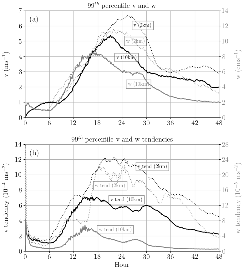
Figure 2 Evolutions of the 99 percentiles of (a) horizontal velocity, v (black; axis on the left), and vertical velocity, w (gray; axis on the right) in the simulation of slantwise convection. Panel (b) is the same as (a) but for their tendencies (black and gray lines for v and w tendencies, respectively). Solid lines are for the 10 km simulation, while the dotted ones are for the 2 km case.

3 Methodology and results

3.1 Inline momentum budget analysis

For the inline budget analysis, all the terms are retrieved directly from the model for all the integration time steps, and therefore they represent the “instantaneous” terms that act over the specified short integration time window. For the large-step forcing, the WRF model accumulates all forcing terms at the beginning of each RK3 step. To separate them, we simply take the difference before and after WRF calls the subroutine for each large-step forcing, store their values separately, and output only the values at the third RK3 step (the total forcing is $F\left({\mathrm{\Phi }}^{**}\right)\mathrm{\Delta }t$ as shown in Fig. 1). As for the contribution of the small-step modes, they are obtained by accumulating over all the small steps in the third RK3 step (ACOUS sum shown in Fig. 1). It is worth noting that Eq. (6) is a vertically implicit equation that couples with the geopotential tendency equation (Skarmarock et al., 2008; Klemp et al., 2007). A tri-diagonal equation for the vector W (involving three grid points in the vertical direction) is thus solved (Satoh, 2002). This means that W (the scalar at a given grid point) is not advanced by linear additions in the small-step or acoustic scheme. To ensure the closure of the inline retrieval budget, we simply take the total changes that are contributed by the implicit solver in the acoustic scheme as small-step modes of W in the third RK3 step. Note that this way does not violate the original W equation in Eq. (6). The contribution from these accumulated small-step modes in the V and W tendency budgets are combined with their large-step PGF and PGFBUOY, respectively, as they share the same mathematical expressions. Finally, we add the inline calculation for the tendency term outside of the RK3 integration loop, after the microphysics scheme:

$$\begin{array}{}\text{(7)}& {{\displaystyle \frac{\partial \mathrm{\Phi }}{\partial t}}}^{t+\mathrm{\Delta }t}\equiv {\displaystyle \frac{{\mathrm{\Phi }}^{t+\mathrm{\Delta }t}-{\mathrm{\Phi }}^t}{\mathrm{\Delta }t}},\end{array}$$

where Δt is the model integration time step and Φ represents V or W (coupled momentum; hereafter the momentum tendency with capital V or W refers to the lhs term derived for the budget analysis). The values of Φ at times t and t+Δt, the latter denoted by superscripts, are termed the current and predicted states, respectively. Note that while variables of momentum tendencies (specifically named “ru_tend, rv_tend and rw_tend”) can be directly outputted from the WRF model by modifying the registry file, these variables do not necessarily represent the actual momentum changes that consider all the physical (e.g., microphysics, small-step modes) and non-physical processes (e.g., damping) but only the summation of all the large-step forcings.

Figures 3 and 4 present the results of the inline budget analysis for horizontal momentum and vertical momentum, respectively, at three selected times (6, 12, and 16 h). To demonstrate the momentum changes in a common physical unit (velocities; meter per second), every term of the flux-form budget equation shown in this paper is divided by the dry-air mass, ${{\mathit{\mu }}_{\mathrm{d}}}^{t+\mathrm{\Delta }t}$ (so that, for example, the V tendency has a unit of meter per second squared). The magnitude of the V tendency intensifies during this period with local maxima on the order of 10⁻⁴ to 10⁻³ m s⁻² (Fig. 3). Two forcing terms, PGF and COR, are a few times larger than the ADV term but generally offset each other, making the ADV term of comparable importance in determining the tendency. The CUV term for V tendency is generally small and thus not shown in Fig. 3. The residual, obtained from Eq. (1) with P_V equal to 0, is always smaller than ${\mathrm{10}}^{-\mathrm{7}}\mathrm{m}{\mathrm{s}}^{-\mathrm{2}}$ during the entire 48 h simulation (not shown). To understand how the peak error evolves with time and to avoid reaching misleading conclusions based on one or more outlying values, the evolution of the 99th percentile magnitude of the residual term is shown. Figure 5 shows that it reaches a value of about $\mathrm{7}\times {\mathrm{10}}^{-\mathrm{9}}$ m s⁻² at around 15 h. Recall that the 99th percentile magnitude of the simulated v tendency has a peak of $\mathrm{7}\times {\mathrm{10}}^{-\mathrm{4}}$ m s⁻² (Fig. 2b). Thus, the relative magnitude of the 99th percentile residual is about 0.001 % of the 99th percentile tendency term during the peak intensifying stage. Compared to the V tendency, the W tendency exhibits narrower features in the horizontal direction (Fig. 4) with an overall smaller magnitude in every term. The two largest forcings, PGFBUOY and CUV, usually have opposite signs, so their combined effect is on the same order as the ADV and the W tendency term. While the contribution from the upper-layer vertical velocity damping is not shown in Fig. 4, it is included as part of the rhs (P_W) of Eq. (2) when calculating the residual for the inline budget analysis. The residual in the inline W budget is generally 4 orders of magnitude smaller than its tendency term. The 99th percentile residual for W budget is about $\mathrm{2}\times {\mathrm{10}}^{-\mathrm{10}}$ m s⁻², around 0.0003 % of the 99th percentile w tendency during the peak intensifying stage of the convection (not shown).

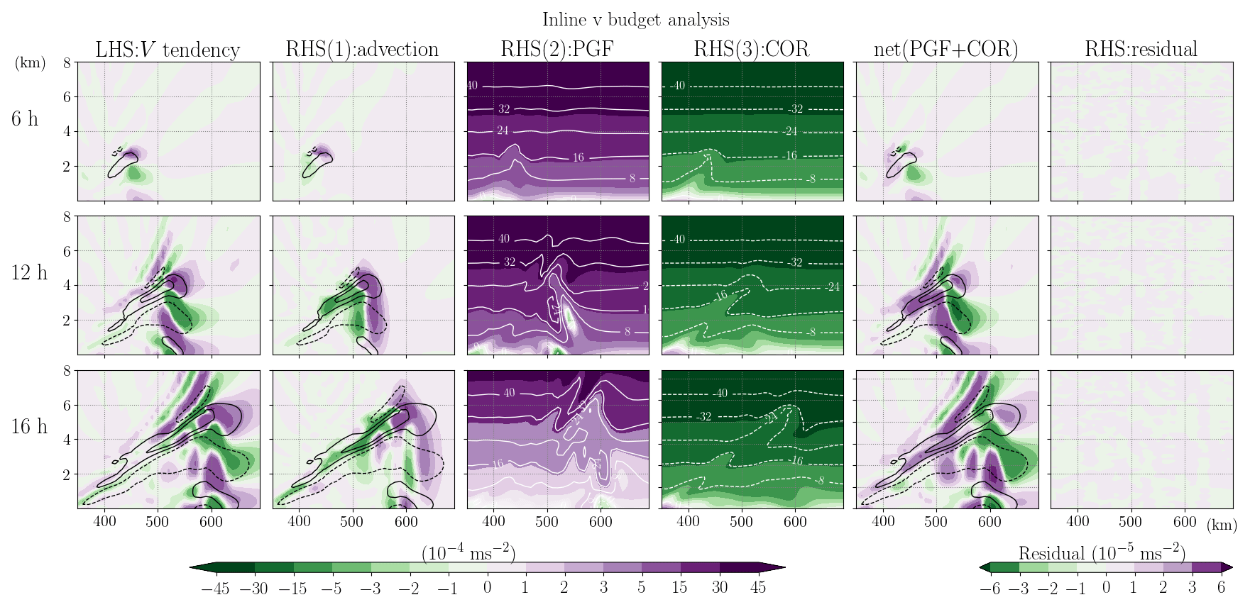
Figure 3 Inline budget analysis of horizontal momentum, V, with each term extracted directly from the model. In each row, the shading in each subplot from the left to right shows the term of V tendency, flux-form advection (ADV), horizontal pressure gradient force (PGF), Coriolis force (COR) (white contours indicate the values exceeding the color bar), PGF+COR, and residual (Eq. 1; P_V is 0 and the generally small curvature term (CUV) is not shown). All terms are divided by μ_d and thus have units of meters per second squared. The black contours indicate the horizontal velocity v of 2 and 6 m s⁻¹ (positive and negative values shown in solid and dashed lines, respectively). Each row from top to bottom illustrates the budget analysis at 6, 12, and 16 h, respectively.

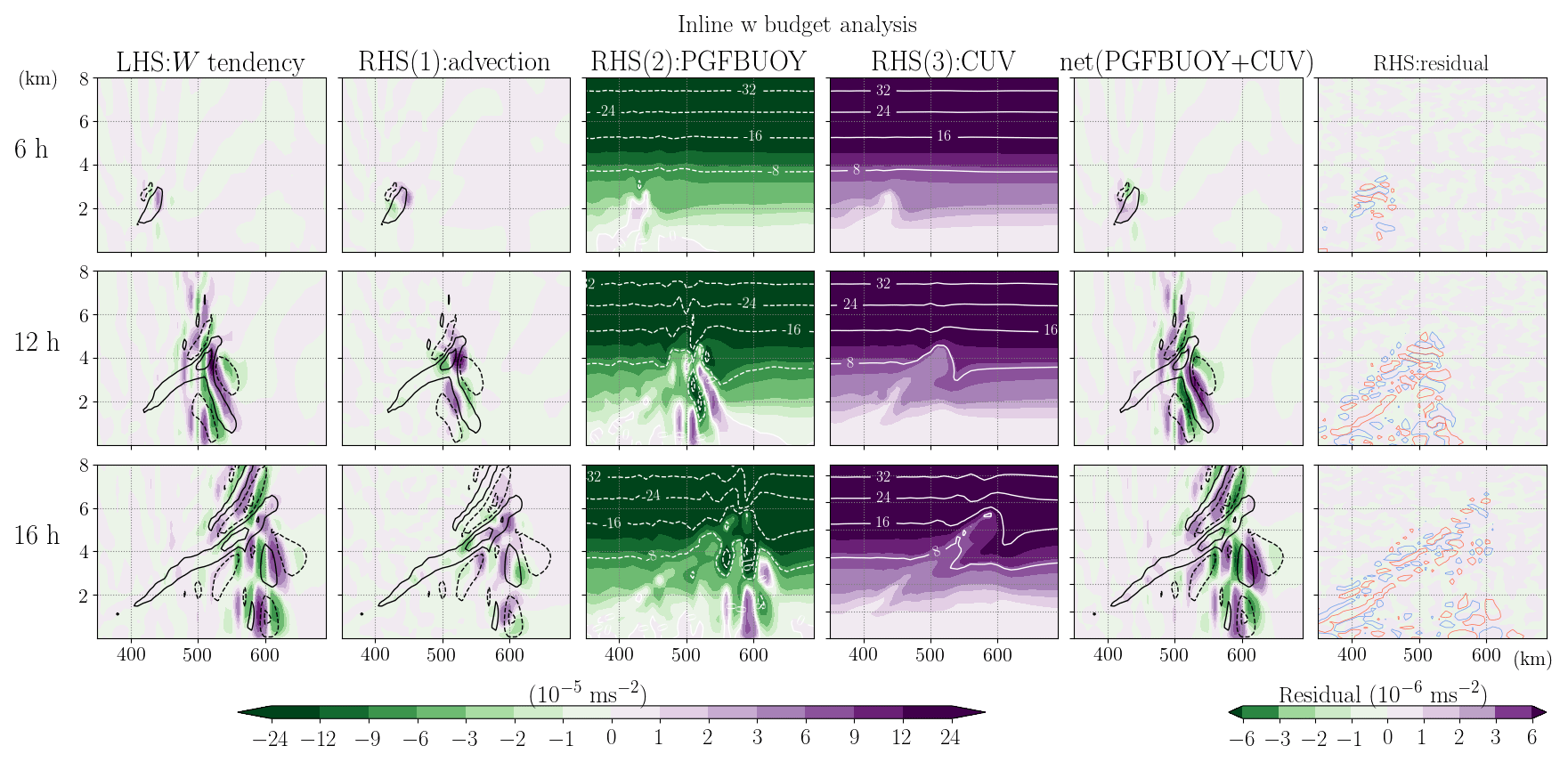
Figure 4 Inline budget analysis of vertical momentum, W, with each term extracted directly from the model. In each row, the shading in each subplot from the left to right shows the term of W tendency, advection (ADV), net vertical pressure gradient and buoyancy force (PGFBUOY), curvature (CUV) (white contours indicate the values exceeding the color bar), PGFBUOY+CUV, and residual (Eq. 2; P_W is considered but not shown here). All terms are divided by μ_d and thus have units of meters per second squared. The black contours indicate the vertical velocity w of 5 and 15 cm s⁻¹ (positive and negative values shown in solid and dashed lines, respectively). The red (blue) contours shown in the rightmost column, laid on top of the residual (shading), indicate the small-step components of PGFBUOY with a positive (negative) value of $\mathrm{3}\times {\mathrm{10}}^{-\mathrm{4}}\mathrm{m}{\mathrm{s}}^{-\mathrm{2}}$. Each row from top to bottom illustrates the budget analysis at 6, 12, and 16 h, respectively.

3.2 Post-processed momentum budget analyses

3.2.1 Key features and methodologies

In contrast to extracting terms directly from the model during its integration, most of the studies in which the momentum budget analysis is conducted use the model output files after the completion of the integration. Note that since the sub-output time-step information is not available between successive outputs, only the large-step forcing terms can be estimated in these post-processed budget analyses. Generally, the neglect of the acoustic or small-step modes is expected to have little impact on the results as the high-frequency modes are often considered meteorologically insignificant. However, it is mentioned in Klemp et al. (2007) and Skamarock et al. (2008) that the WRF small-step integration scheme includes not only the acoustic-wave but also some gravity-wave modes, which may not be insignificant. These gravity-wave modes form during the small-step integration due to the designated terms that are required for acoustic-wave propagation and “Consequently, in this vertical coordinate (i.e., terrain-following hydrostatic pressure coordinate), the terms governing the acoustic and gravity wave modes are intermingled to the extent that it does not appear feasible to evaluate any of the gravity wave terms on the large time steps, even if one desired to do so” (Klemp et al., 2007).

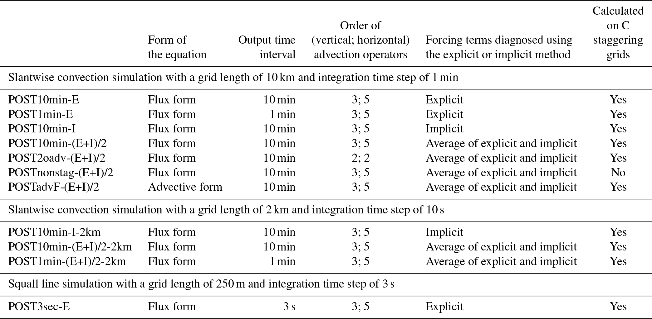
Most of the studies did not reveal the complete details about how their analysis was done, so we cannot presume their methodologies and the possible errors. However, a few simplifications commonly made in the post-processed budget analyses may introduce errors that result in deviations from the simulated results and thus a significant residual. Below we revisit the relevant features of the WRF model that should be considered and discuss how they might affect the post-processed budget if they are ignored. Then, the results are shown for different post-processed budget analyses with different simplifications (Table 1). The aim herein is to identify these potential errors hidden in the budget calculation and show how severely they affect the resulting interpretation.

Table 1 A summary of all different approaches for the post-processed horizontal momentum budget analysis that are applied to the model output after the integration finishes.

(a) Diagnosed tendency

In a post-processed budget analysis, the tendency term of a given variable is approximated by the difference between the value of this variable at two successive output times divided by the output time interval. Thus, the accuracy may be sensitive to the output time interval. The value at the predicted state has a form of

$$\begin{array}{}\text{(8)}& {\left.{{\displaystyle \frac{\partial \mathrm{\Phi }}{\partial t}}}^{t+\mathrm{\Delta }t}\right|}_{\mathrm{diagnosed}}\approx {\displaystyle \frac{{\mathrm{\Phi }}^{t+\mathrm{\Delta }t}-{\mathrm{\Phi }}^{t+\mathrm{\Delta }t-\mathrm{\Delta }{t}_{\mathrm{output}}}}{\mathrm{\Delta }{t}_{\mathrm{output}}}}.\end{array}$$

If the output interval is longer than the model integration time step, the diagnosed tendency would deviate from the model prediction of the instantaneous tendency. To increase the accuracy, the output time interval Δt_output needs to be similar to the integration time step Δt.

(b) Spatial discretization on the C staggered grid

For computational efficiency and accuracy, WRF utilizes a C-grid staggering system (Arakawa and Lamb, 1977). This staggering system is pertinent to the numerical solution for spatial derivatives. For most of the spatial derivatives other than advection (e.g., the pressure gradient force), the second-order finite difference operator is used in the WRF model. For example, the y derivative of variable Φ is calculated using the discrete operator:

$$\begin{array}{}\text{(9)}& {{\displaystyle \frac{\partial \mathrm{\Phi }}{\partial y}}}_{i,j,k}={\displaystyle \frac{\mathrm{1}}{\mathrm{\Delta }y}}\left({\mathrm{\Phi }}_{i,j+\frac{\mathrm{1}}{\mathrm{2}},k}-{\mathrm{\Phi }}_{i,j-\frac{\mathrm{1}}{\mathrm{2}},k}\right).\end{array}$$

The index ($i,j,k$) corresponds to a location with $(x,y,\mathit{\eta })=(i\mathrm{\Delta }x,j\mathrm{\Delta }y,k\mathrm{\Delta }\mathit{\eta })$, where Δx, Δy and Δη are the grid lengths in the two horizontal and vertical directions (can be vertically stretched), respectively. The same expression applies for the x or the η derivatives. Grid staggering implies that different variables may be located on different grids, i.e., shifted by a half-grid point from the others as illustrated in Fig. 6. Depending on what variable the spatial derivatives are intended for, Eq. (9) should be carried out on the corresponding grid, which is not necessarily the same as the Φ grid. For example, for the V tendency, all the associated forcing terms involving the spatial derivatives should be performed on the V grid. More specifically, to calculate the PGF term for the V tendency equation, the term $\frac{\partial p}{\partial y}$ and the term $\frac{\partial p}{\partial \mathit{\eta }}$ in Eq. (1) should be calculated on the V grid but not the pressure grid (p grid). Applying Eq. (9) for $\frac{\partial p}{\partial y}$, the V grid with location indices of $(i,j-\frac{\mathrm{1}}{\mathrm{2}},k$) and $(i,j+\frac{\mathrm{1}}{\mathrm{2}},k$) falls exactly on the p grid and hence no interpolation is required (red arrows in Fig. 6a). However, for $\frac{\partial p}{\partial \mathit{\eta }}$, the pressures on the V grid with indices of $(i,j,k-\frac{\mathrm{1}}{\mathrm{2}}$) and $(i,j,k+\frac{\mathrm{1}}{\mathrm{2}}$) must be obtained (red arrows in Fig. 6b) through linear interpolation using their surrounding closest four pressure values, e.g.,

$$\begin{array}{}\text{(10)}& \begin{array}{rl}& p_{V\text{-}\mathrm{grid}\left(i,j,k+\frac{\mathrm{1}}{\mathrm{2}}\right)}\\ & ={\displaystyle \frac{\frac{\mathrm{1}}{\mathrm{2}}\left(p_{p\text{-}\mathrm{grid}\left(i,j-\mathrm{1},k\right)}+p_{p\text{-}\mathrm{grid}\left(i,j,k\right)}\right)\frac{\mathrm{\Delta }{\mathit{\eta }}_{k+\mathrm{1}}}{\mathrm{2}}}{\frac{\mathrm{1}}{\mathrm{2}}\left(\mathrm{\Delta }{\mathit{\eta }}_k+\mathrm{\Delta }{\mathit{\eta }}_{k+\mathrm{1}}\right)}}\\ & +{\displaystyle \frac{\frac{\mathrm{1}}{\mathrm{2}}\left(p_{p\text{-}\mathrm{grid}\left(i,j-\mathrm{1},k+\mathrm{1}\right)}+p_{p\text{-}\mathrm{grid}\left(i,j,k+\mathrm{1}\right)}\right)\frac{\mathrm{\Delta }{\mathit{\eta }}_k}{\mathrm{2}}}{\frac{\mathrm{1}}{\mathrm{2}}(\mathrm{\Delta }{\mathit{\eta }}_k+\mathrm{\Delta }{\mathit{\eta }}_{k+\mathrm{1}})}},\end{array}\end{array}$$

which is weighted by the irregular (stretched) vertical grid-lengths (Fig. 6b).

Figure 5 Evolution of the 99th percentile of the residual magnitude (meters per second squared) of the horizontal momentum V budget analysis. For the residual calculation, (a) uses the true V tendency (derived during the integration of the model) and (b) uses the post-diagnosed V tendency (Eq. 8) as the lhs term. Different colors indicate different post-processed methods for estimating the rhs forcing terms. The residuals obtained from the inline budget retrieval are in black. Solid and dashed lines are for the 10 km run and 2 km run, respectively.

Figure 6 (a) Horizontal and (b) vertical C staggering grids for different variables in the WRF model. Note that variables ϕ and W are allocated on the same grid as Ω; μ, α, and q_* are on grid same as p. The red arrows indicate the grids that would be used to calculate the second-order spatial derivative term for the V momentum at the V grid (i, j, k).

If the C-grid staggering is not considered during the post-processing analysis, i.e., all the variables have been interpolated on the universal grids before carrying out the budget calculation, in addition to the potential errors brought on by the interpolation method, the term $\frac{\partial p}{\partial y}$, for example, would essentially involve pressure differences over a larger grid interval of 2×Δy instead of Δy, with larger associated truncation errors.

(c) Advection operators

For advection, higher-order operators for finite differencing are provided as the default WRF setup. Taking the y component of the flux-form advection for V momentum in Eq. (3) as an example, with a fifth-order operator as selected in the present simulation, it is written as

$$\begin{array}{}\text{(11)}& \begin{array}{rl}-{{\displaystyle \frac{\partial \left(Vv\right)}{\partial y}}}_{i,j,k}& \approx -{\displaystyle \frac{\mathrm{1}}{\mathrm{\Delta }y}}\left(V_{i,j+\frac{\mathrm{1}}{\mathrm{2}},k}{v}_{i,j+\frac{\mathrm{1}}{\mathrm{2}},k}^{\mathrm{5}\mathrm{th}}\right.\\ & \left.-V_{i,j-\frac{\mathrm{1}}{\mathrm{2}},k}{v}_{i,j-\frac{\mathrm{1}}{\mathrm{2}},k}^{\mathrm{5}\mathrm{th}}\right),\end{array}\end{array}$$

where V and v are the mass-coupled and mass-uncoupled velocities, respectively:

$$\begin{array}{rl}{v}_{i,j-\frac{\mathrm{1}}{\mathrm{2}},k}^{\mathrm{5}\mathrm{th}}& =v_{i,j-\frac{\mathrm{1}}{\mathrm{2}},k}^{\mathrm{6}\mathrm{th}}-\mathrm{sign}\left(V_{i,j-\frac{\mathrm{1}}{\mathrm{2}},k}\right){\displaystyle \frac{\mathrm{1}}{\mathrm{60}}}\\ & \left[\left(v_{i,j+\mathrm{2},k}-v_{i,j-\mathrm{3},k}\right)-\mathrm{5}\left(v_{i,j+\mathrm{1},k}-v_{i,j-\mathrm{2},k}\right)\right.\\ & \left.+\mathrm{10}\left(v_{i,j,k}-v_{i,j-\mathrm{1},k}\right)\right]\end{array}$$

and

$$\begin{array}{rl}{v}_{i,j-\frac{\mathrm{1}}{\mathrm{2}},k}^{\mathrm{6}\mathrm{th}}& ={\displaystyle \frac{\mathrm{1}}{\mathrm{60}}}[\mathrm{37}\left(v_{i,j,k}-v_{i,j-\mathrm{1},k}\right)\\ & -\mathrm{8}\left(v_{i,j+\mathrm{1},k}+v_{i,j-\mathrm{2},k}\right)\\ & +\mathrm{1}\left(v_{i,j+\mathrm{2},k}+v_{i,j-\mathrm{3},k}\right)].\end{array}$$

The odd-order advection operators include a spatially centered even-order operator and an upwind diffusion term. A detailed discussion on the advection scheme in the WRF model with different-order operators can be found in Wicker and Skamarock (2002) and Skamarock et al. (2008). Simplifying the advection estimation using an operator with an order that differs from the numerical setup would contribute to errors in the ADV estimation.

(d) Forward or backward Euler method

Conceptually, the WRF model can be considered more of a forward scheme, i.e., using the known variables from the current state to calculate the forcing and then advancing the variables forward until reaching the prediction time. However, there are a few implicit components during the integration. For example, as discussed in Sect. 2.1, the large-step forcings are updated using a predictor–corrector method in the second and third RK3 steps. In addition, the W equation is coupled with the geopotential tendency equation and includes a forward-in-time weighting that utilizes predicted states of the geopotential and temperature in solving the W (Eq. 3.11, 3.12, and 3.19 in Skamarock et al., 2008).

In numerical analysis for solving ordinary differential equations, the (explicit) forward Euler method approximates the change of a system from t to t+Δt using the current states (t), while the (implicit) backward Euler method finds the solution using the predicted states (t+Δt):

$$\begin{array}{}\text{(12)}& {{\displaystyle \frac{\partial \mathrm{\Phi }}{\partial t}}}^{t+\mathrm{\Delta }t}\approx F\left({\mathrm{\Phi }}^t\right)\mathrm{forward}\mathrm{Euler}\mathrm{method},\text{(13)}& {{\displaystyle \frac{\partial \mathrm{\Phi }}{\partial t}}}^{t+\mathrm{\Delta }t}\approx F\left({\mathrm{\Phi }}^{t+\mathrm{\Delta }t}\right)\mathrm{backward}\mathrm{Euler}\mathrm{method}.\end{array}$$

Consistent with this concept, the rhs forcing terms of a budget equation can be estimated using two different instantaneous states in analogous ways. However, we emphasize that the post-processed budget analysis does not solve the tendency equation per se but only diagnoses the relationship between the two sides of the equation. Note that for post-processing analyses, the availability of the data depends on the output time interval (Δt_output), which is often much larger than the integration time step (Δt). Thus, for the tendency at a given time t+Δt, when applying the forward Euler method to estimate the associated rhs forcings, the “current states” one can use are the most recent prior output at $t+\mathrm{\Delta }t-\mathrm{\Delta }{t}_{\mathrm{output}}$ (see Fig. 7):

$$\begin{array}{}\text{(14)}& \begin{array}{rl}& {{\displaystyle \frac{\partial \mathrm{\Phi }}{\partial t}}}^{t+\mathrm{\Delta }t}\approx F\left({\mathrm{\Phi }}^{t+\mathrm{\Delta }t-\mathrm{\Delta }{t}_{\mathrm{output}}}\right)\mathrm{forward}\mathrm{Euler}\mathrm{method}\\ & \mathrm{for}\mathrm{post}\text{-}\mathrm{processing}.\end{array}\end{array}$$

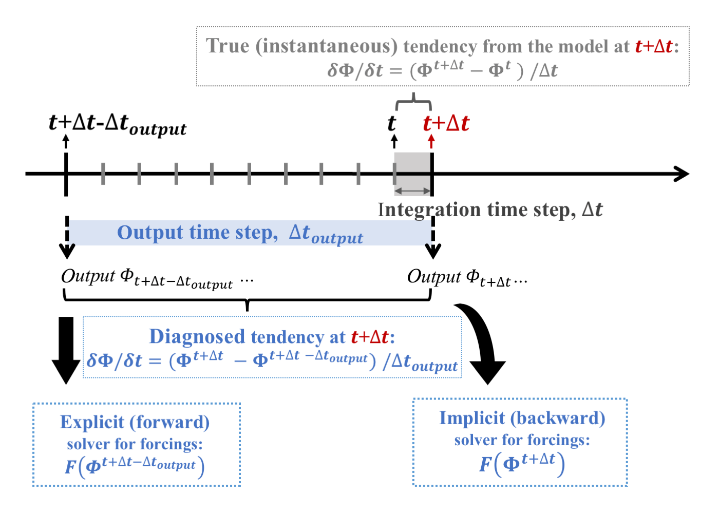
Figure 7 Schematic plot showing the explicit (forward) and implicit (backward) solvers for the rhs forcing terms, as well as the diagnosed and the true (calculated inline during the integration of the model) lhs tendency term defined in this study.

If Δt_output is the same as Δt, Eq. (14) reverts to Eq. (12). If Δt_output is much larger than Δt, the backward Euler method using predicted states at t+Δt may better estimate the true model forcing terms as they are calculated using variables at a closer time to the real integration window in the model (Fig. 7).

The above two diagnostic methods estimate the forcing terms using instantaneous states. However, as mentioned in Sect. 3.2.1(a), the diagnosed lhs tendency depends on two successive model output times. Thus, an average between forcings diagnosed explicitly and implicitly are often considered. For a post-processed analysis, this translates into estimating the forcings using both predicted states and the most recent prior available current states:

$$\begin{array}{}\text{(15)}& {\left.{{\displaystyle \frac{\partial \mathrm{\Phi }}{\partial t}}}^{t+\mathrm{\Delta }t}\right|}_{\mathrm{diagnosed}}\approx {\displaystyle \frac{\mathrm{1}}{\mathrm{2}}}\left[F\left({\mathrm{\Phi }}^{t+\mathrm{\Delta }t-\mathrm{\Delta }{t}_{\mathrm{output}}}\right)+F\left({\mathrm{\Phi }}^{t+\mathrm{\Delta }t}\right)\right].\end{array}$$

(e) Flux or advective form of equation

While the momentum equations solved in the WRF model are in flux form, their corresponding advective forms can be derived and are often used for post-processed budget analyses for convenience. To derive the advective form, the flux-form V momentum equation (Eq. 1 excluding residual) is first multiplied by a factor of $\frac{\mathrm{1}}{{\mathit{\mu }}_{\mathrm{d}}}$ and V is rewritten as μ_dv:

$$\begin{array}{}\text{(16)}& \begin{array}{rl}\underset{V\mathrm{tendency}}{\underbrace{{\displaystyle \frac{\mathrm{1}}{{\mathit{\mu }}_{\mathrm{d}}}}{\displaystyle \frac{\partial \left({\mathit{\mu }}_{\mathrm{d}}v\right)}{\partial t}}}}& =\underset{\begin{array}{c}\mathrm{advection}\\ \mathrm{ADV}\end{array}}{\underbrace{-{\displaystyle \frac{\mathrm{1}}{{\mathit{\mu }}_{\mathrm{d}}}}\mathrm{\nabla }\cdot \left({\mathit{\mu }}_{\mathrm{d}}\mathit{v}v\right)}}\\ & \underset{\begin{array}{c}\mathrm{horizontal}\mathrm{pressure}\mathrm{gradient}\mathrm{force}\\ \mathrm{PGF}\end{array}}{+\underbrace{{\displaystyle \frac{\mathrm{1}}{{\mathit{\mu }}_{\mathrm{d}}}}\left[-\mathit{\alpha }{\displaystyle \frac{\partial p}{\partial y}}-{\displaystyle \frac{\mathit{\alpha }}{{\mathit{\alpha }}_{\mathrm{d}}}}{\displaystyle \frac{\partial p}{\partial \mathit{\eta }}}{\displaystyle \frac{\partial \mathit{\varphi }}{\partial y}}\right]}}\\ & \underset{\begin{array}{c}\mathrm{Coriolis}\\ \mathrm{COR}\end{array}}{\underbrace{-{\displaystyle \frac{\mathrm{1}}{{\mathit{\mu }}_{\mathrm{d}}}}fU}}\underset{\begin{array}{c}\mathrm{curvature}\\ \mathrm{CUV}\end{array}}{\underbrace{-{\displaystyle \frac{\mathrm{1}}{{\mathit{\mu }}_{\mathrm{d}}}}\left({\displaystyle \frac{vW}{r_{\mathrm{e}}}}\right)}}+\underset{\begin{array}{c}\mathrm{remaining}\\ \left(\mathrm{parameterized}\right)\\ \mathrm{physics}\end{array}}{\underbrace{{\displaystyle \frac{\mathrm{1}}{{\mathit{\mu }}_{\mathrm{d}}}}{P}_V}}.\end{array}\end{array}$$

Then, by adding the mass continuity equation in WRF (multiplied by a factor of $\frac{v}{{\mathit{\mu }}_{\mathrm{d}}}$):

$${\displaystyle \frac{v}{{\mathit{\mu }}_{\mathrm{d}}}}\left[{\displaystyle \frac{\partial {\mathit{\mu }}_{\mathrm{d}}}{\partial \mathrm{t}}}+\mathrm{\nabla }\cdot \left({\mathit{\mu }}_{\mathrm{d}}\mathit{v}\right)\right]=\mathrm{0}$$

to the rhs of Eq. (16), we obtain

$$\begin{array}{}\text{(17)}& \begin{array}{rl}\underset{V\mathrm{tendency}}{\underbrace{{\displaystyle \frac{\mathrm{1}}{{\mathit{\mu }}_{\mathrm{d}}}}{\displaystyle \frac{\partial \left({\mathit{\mu }}_{\mathrm{d}}v\right)}{\partial t}}}}& ={\displaystyle \frac{v}{{\mathit{\mu }}_{\mathrm{d}}}}{\displaystyle \frac{\partial {\mathit{\mu }}_{\mathrm{d}}}{\partial t}}+{\displaystyle \frac{v}{{\mathit{\mu }}_{\mathrm{d}}}}\mathrm{\nabla }\cdot \left({\mathit{\mu }}_{\mathrm{d}}\mathit{v}\right)\underset{\begin{array}{c}\mathrm{advection}\\ \mathrm{ADV}\end{array}}{\underbrace{-{\displaystyle \frac{\mathrm{1}}{{\mathit{\mu }}_{\mathrm{d}}}}\mathrm{\nabla }\cdot \left({\mathit{\mu }}_{\mathrm{d}}\mathit{v}v\right)}}\\ & \underset{\begin{array}{c}\mathrm{horizontal}\mathrm{pressure}\mathrm{gradient}\mathrm{force}\\ \mathrm{PGF}\end{array}}{\underbrace{+{\displaystyle \frac{\mathrm{1}}{{\mathit{\mu }}_{\mathrm{d}}}}\left[-\mathit{\alpha }{\displaystyle \frac{\partial p}{\partial y}}-{\displaystyle \frac{\mathit{\alpha }}{{\mathit{\alpha }}_{\mathrm{d}}}}{\displaystyle \frac{\partial p}{\partial \mathit{\eta }}}{\displaystyle \frac{\partial \mathit{\varphi }}{\partial y}}\right]}}\underset{\begin{array}{c}\mathrm{Coriolis}\\ \mathrm{COR}\end{array}}{\underbrace{-{\displaystyle \frac{\mathrm{1}}{{\mathit{\mu }}_{\mathrm{d}}}}fU}}\\ & \underset{\begin{array}{c}\mathrm{curvature}\\ \mathrm{CUV}\end{array}}{\underbrace{-{\displaystyle \frac{\mathrm{1}}{{\mathit{\mu }}_{\mathrm{d}}}}\left({\displaystyle \frac{vW}{r_{\mathrm{e}}}}\right)}}+\underset{\begin{array}{c}\mathrm{remaining}\\ \left(\mathrm{parameterized}\right)\\ \mathrm{physics}\end{array}}{\underbrace{{\displaystyle \frac{\mathrm{1}}{{\mathit{\mu }}_{\mathrm{d}}}}{P}_V}}.\end{array}\end{array}$$

Moving the first term on the rhs of Eq. (17) to the lhs, the second rhs term can be combined with the flux-form advection using the vector identity $\mathrm{\nabla }\cdot \left({\mathit{\mu }}_{\mathrm{d}}\mathit{v}\right)={\mathit{\mu }}_{\mathrm{d}}\left(\mathrm{\nabla }\cdot \mathit{v}\right)+\mathit{v}\cdot \left(\mathrm{\nabla }{\mathit{\mu }}_{\mathrm{d}}\right)$. Then, the advective form of the horizontal momentum equation is obtained as

$$\begin{array}{}\text{(18)}& \begin{array}{rl}\underset{\begin{array}{c}v\mathrm{tendency}\\ \mathrm{in}\mathrm{advective}\mathrm{form}\end{array}}{\underbrace{{\displaystyle \frac{\partial v}{\partial t}}}}& =\underset{\begin{array}{c}\mathrm{advection}\mathrm{ADV}\\ \mathrm{in}\mathrm{advective}\mathrm{form}\end{array}}{\underbrace{-\mathit{v}\cdot \mathrm{\nabla }v}}\\ & \underset{\begin{array}{c}\mathrm{horizontal}\mathrm{pressure}\mathrm{gradient}\mathrm{force}\\ \mathrm{PGF}\end{array}}{\underbrace{+{\displaystyle \frac{\mathrm{1}}{{\mathit{\mu }}_{\mathrm{d}}}}\left[-\mathit{\alpha }{\displaystyle \frac{\partial p}{\partial y}}-{\displaystyle \frac{\mathit{\alpha }}{{\mathit{\alpha }}_{\mathrm{d}}}}{\displaystyle \frac{\partial p}{\partial \mathit{\eta }}}{\displaystyle \frac{\partial \mathit{\varphi }}{\partial y}}\right]}}\\ & \underset{\begin{array}{c}\mathrm{Coriolis}\\ \mathrm{COR}\end{array}}{\underbrace{-{\displaystyle \frac{\mathrm{1}}{{\mathit{\mu }}_{\mathrm{d}}}}fU}}\underset{\begin{array}{c}\mathrm{curvature}\\ \mathrm{CUV}\end{array}}{\underbrace{-{\displaystyle \frac{\mathrm{1}}{{\mathit{\mu }}_{\mathrm{d}}}}\left({\displaystyle \frac{vW}{r_{\mathrm{e}}}}\right)}}\\ & +\underset{\begin{array}{c}\mathrm{remaining}\\ \left(\mathrm{parameterized}\right)\\ \mathrm{physics}\end{array}}{\underbrace{{\displaystyle \frac{\mathrm{1}}{{\mathit{\mu }}_{\mathrm{d}}}}{P}_V}}.\end{array}\end{array}$$

3.2.2 Results of horizontal momentum budget

Table 1 summarizes all the post-processed budget analyses tested in this study. In the present section, we first present the results one by one, and then a qualitative intercomparison among them and the inline retrieval method is discussed. The first post-processed method (POST10min-E) for V budget follows all the approaches in the model as closely as possible using the 10 min output data. The flux-form equation, C staggering grids, and the same orders of advection operators as the experimental setup are used. The diagnosis of the large-step forcing is applied directly to the model outputs on η levels using the explicit or forward Euler method as shown in Eq. (14). The diagnosed forcing terms are compared with their corresponding true values from the inline retrieval (Fig. 8). Errors smaller than, but on the same order of 10⁻⁴ m s⁻² as the V tendency, are observed in all terms including the diagnosed tendency term. These errors grow in magnitude and areal coverage with the growth of the disturbance. Aside from COR, the absolute errors in the tendency, ADV and PGF can exceed $\mathrm{6}\times {\mathrm{10}}^{-\mathrm{4}}$ m s⁻², the former two of which are more than 50 % of the magnitude of their true (instantaneous) values locally.

Figure 8 The difference between the post-processed (POST10min-E; with an explicit or forward method on 10 min output) and inline budget analysis for the horizontal momentum, V. All terms have been divided by μ_d and thus have a uniform unit of meters per second squared. In each row, from left to right indicates the difference for V tendency, ADV, PGF, and COR. The rightmost column indicates the residual term obtained in the post-processed budget analysis. Each row from top to bottom shows the results at 6, 12, and 16 h, respectively.

The second post-processed analysis (POST1min-E) is done following the same approach but applied to the 1 min (same as the integration time step for this simulation) output data, and the results show strongly reduced errors in all terms (Fig. 9). The errors that remain are mostly in the PGF term and likely stem from the fact that the small-step modes and the RK3 integration scheme are not considered in the post-processed budget. These inherent errors result in a small residual term with a general order of 10⁻⁵ m s⁻², 1 to 2 order(s) smaller than the maximum V tendency. In terms of local maxima, the 99th percentile magnitude of the residual obtained in POST1min-E gives a relative magnitude of about 7 % of the 99th percentile v tendency during the peak intensifying stage of the convection at around 15 h (Figs. 2b and 5). Although reducing the model output interval to be close to the integration time step helps to balance the budget without the need for inline diagnoses, it is computationally expensive especially for large, data-intensive simulations.

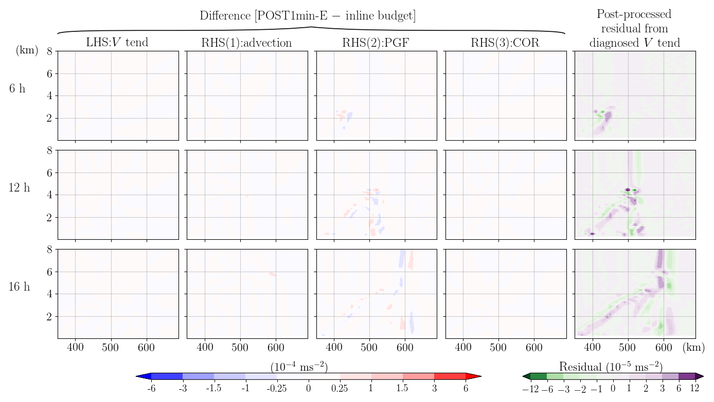
Figure 9 Same as Fig. 8, but the post-processed budget analysis is applied to the data with an output time interval of 1 min (POST1min-E).

Given that computational cost is often a major consideration, we also test whether the implicit or backward Euler method (POST10min-I) can improve the estimation of instantaneous forcing terms relative to the explicit method for the same 10 min output data (POST10min-E). POST10min-I follows the same strategy as POST10min-E except that all the rhs terms, following Eq. (13), are diagnosed with the predicted states instead of the previous output states. As depicted in Fig. 10, POST10min-I does indeed better capture the true model estimated forcing values as errors in all the rhs forcing terms diminish greatly to an accuracy similar to POST1min-E. However, as these forcings are calculated at a given instant, the imbalance of the budget would remain if the diagnosed tendency term is not calculated instantaneously (the second column from the right in Fig. 10). Therefore, if budget analysis at an instant of time is desired, we recommend adding the tendency calculation within the model as a standard output and diagnosing the forcing terms implicitly, which yields a residual term on a similar order to the one obtained in POST1min-E (the rightmost column in Fig. 10 and Fig. 5a).

Figure 10 Same as Fig. 8, but the post-processed rhs terms are diagnosed using the implicit or backward method (POST10min-I) and an extra column is added on the rightmost showing the residual from the true tendency (i.e., the instantaneous value obtained from the model).

For the more common situation, the post-processed analyses diagnose rhs terms using two successive outputs over an output time interval, i.e., taking the averages of the explicitly and implicitly calculated forcings using Eq. (15) on the 10 min output (POST10min-(E+I)/2). Comparing the averaged rhs forcings with the analogously diagnosed lhs momentum tendency (Eq. 8) gives a small residual to a similar accuracy level as POST1min-E and POST10min-I (the rightmost column in Figs. 11 and 5b).

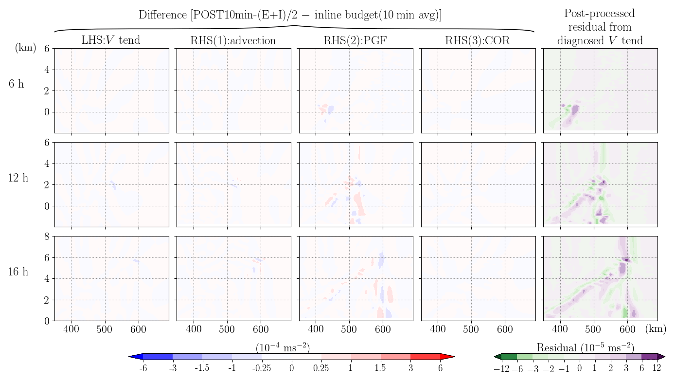
Figure 11 Same as Fig. 8, but the forcing terms diagnosed in the post-processed budget analysis are the averages of explicit and implicit methods (POST10min-(E+I)/2). To represent the same time window as the post-processed analysis, the inline budget results used here for the difference calculation are the 10 min averages (corresponding to the output interval) instead of the instantaneous values.

We now investigate the impact of other common simplifications on top of the reference experiment, POST10min-(E+I)/2. The first such simplification is to approximate the flux-form advection term using the second-order operator (Eq. 9) for both vertical and horizontal components (POST2oadv-(E+I)/2) instead of the third- and fifth-order operators as used in the model setup. In our simulation, such inconsistency of advection operators introduced errors in the ADV term with a maximum value $>\mathrm{3}\times {\mathrm{10}}^{-\mathrm{4}}$ m s⁻², more than 50 % of its true magnitude along the slantwise convective band (Fig. 12). Next, we repeated POST10min-(E+I)/2 but the calculation is applied after all the model output variables have been interpolated to the universal or un-staggered grid (pressure grid) (POSTnonstag-(E+I)/2). This is a common way to post-process model output data for plotting purposes. As mentioned earlier, this approach would reduce the accuracy when solving the spatial differential terms, and indeed, the results do indicate significant errors over a large area in both ADV and PGF (Fig. 13). Their combined errors result in widespread residual values $>\mathrm{3}\times {\mathrm{10}}^{-\mathrm{5}}$ m s⁻² even over the area where the tendency term is smaller than $\mathrm{1}\times {\mathrm{10}}^{-\mathrm{4}}$ m s⁻² (error is at least of 30 % magnitude of the tendency term over a wide area and is reaching 100 % over the band head).

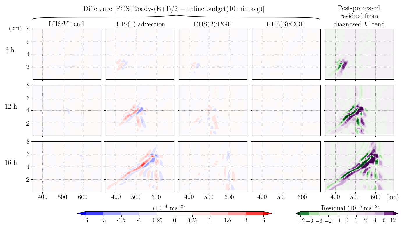
Figure 12 Same as Fig. 11, but the post-processed analysis uses a second-order operator for advection calculation (POST2oadv-(E+I)/2).

Finally, a different format of the V equation, the advective form, is used for post-processed analysis (POSTadvF-(E+I)/2). Mathematically, the flux-from momentum equation can be rewritten in the advective form without making any additional approximation, only with the aid of the conservation law of dry-air mass in the WRF model as shown in Eqs. (16)–(18). However, during the interchange of the expression for the tendency and advection terms, truncation errors may be introduced. We reiterate that the tendency term in the advective form is not equivalent to the one in the flux form divided by μ_d; however, calculation suggests that they are approximately equal, i.e.,

$${\displaystyle \frac{\mathrm{1}}{{\mathit{\mu }}_{\mathrm{d}}}}{\displaystyle \frac{\partial \left({\mathit{\mu }}_{\mathrm{d}}v\right)}{\partial t}}\approx {\displaystyle \frac{\partial v}{\partial t}},$$

with a maximum error that is on the order of ${\mathrm{10}}^{-\mathrm{7}}\sim {\mathrm{10}}^{-\mathrm{8}}$ m s⁻² (3 orders of magnitude smaller than the simulated v tendency) in our study. The summation of the tendency term and advection term in these two forms of the momentum equation should be mathematically identical, so we would expect to see a small difference in the advection term as in the tendency term. However, we find that the advection term in the advective form has a strong positive bias compared to that in the flux form (Fig. 14). The residual term in the POSTadvF-(E+I)/2 is thus negatively biased over the entire convective band with a magnitude exceeding $\mathrm{1.2}\times {\mathrm{10}}^{-\mathrm{4}}$ m s⁻² (reaching 100 % error near the upper half of the convective band). If the residual is neglected or not shown, authors and/or readers may falsely consider the advection process to be the dominant term governing the evolution of the slantwise updraft.

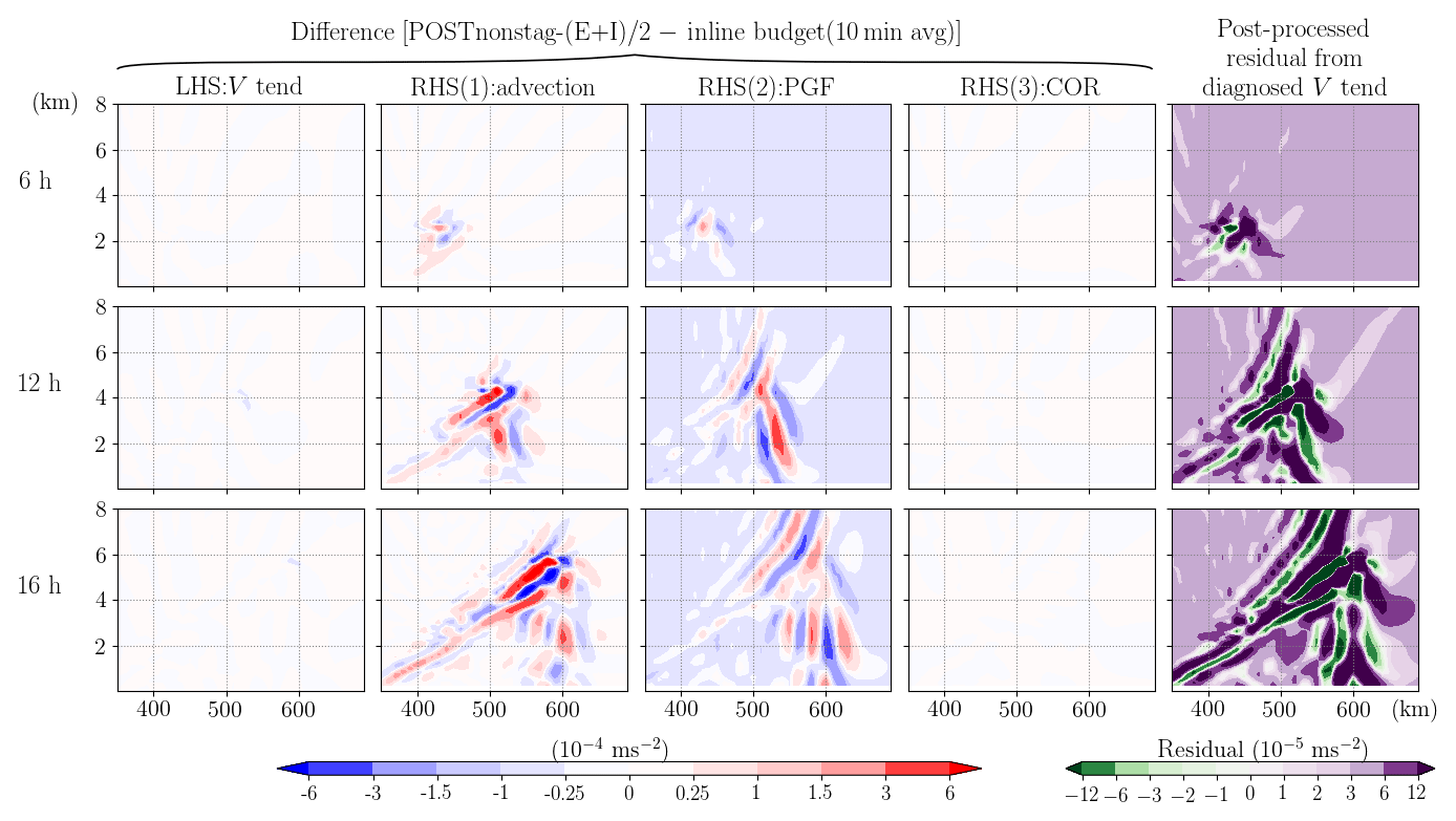
Figure 13 Same as Fig. 11, but the post-processed analysis does not consider C staggering grids (POSTnonstag-(E+I)/2).

Figure 14 Same as Fig. 11, but the post-processed analysis is applied using the advective-form equation (POSTadvF-(E+I)/2).

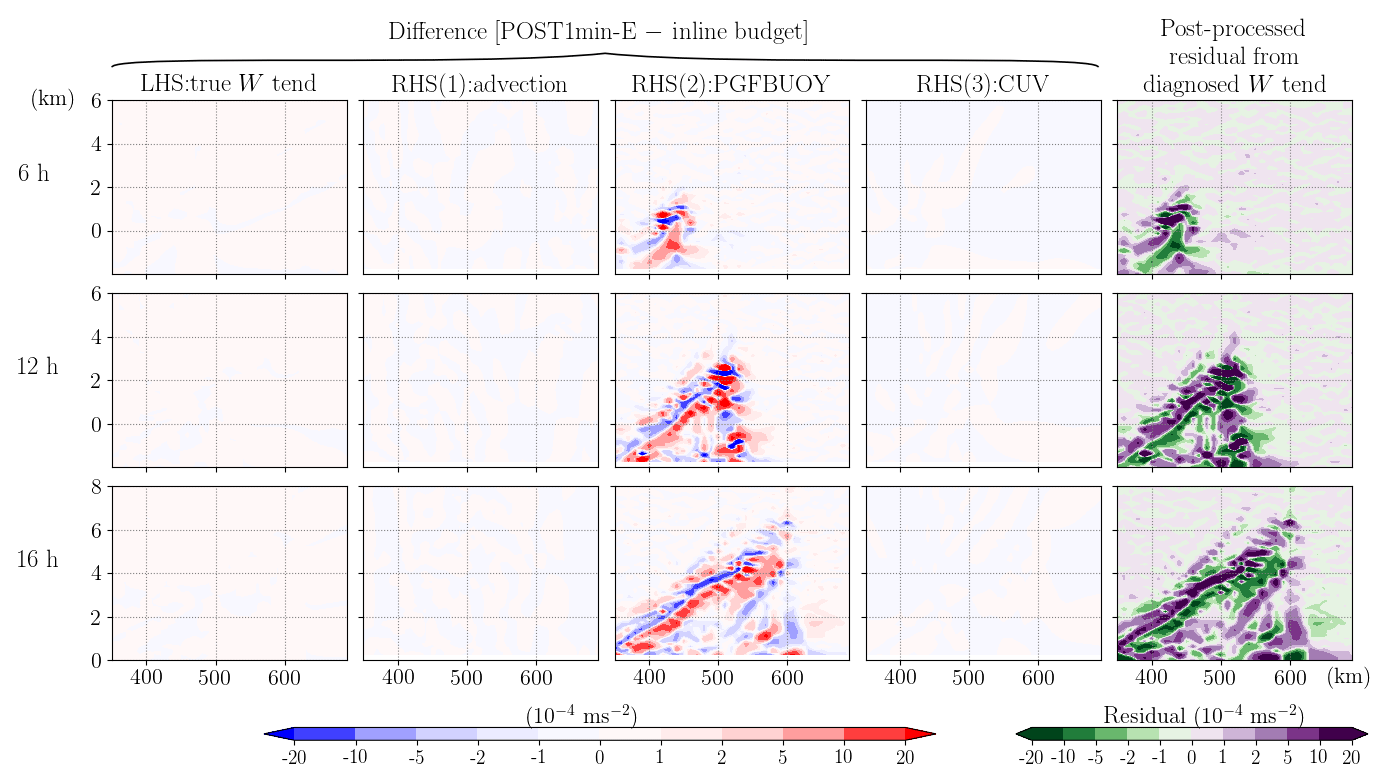
Figure 15 The difference between the post-processed (POST1min-E) and the inline budget analysis for vertical momentum W. All terms have been divided by μ_d and thus have a uniform unit of meters per second squared. In each row, the subplots from left to right indicate the difference of true W tendency, ADV, PGFBUOY, and CUV. The rightmost subplot indicates the residual term obtained in the post-processed budget analysis. Each row from top to bottom shows the results at 6, 12, and 16 h, respectively.

A quantitative comparison of the 99th percentile of the magnitude of the residual term in the domain (excluding the boundaries) among different analysis methods is shown in Fig. 5. The residuals between the instantaneously diagnosed forcings and the true model tendency term (calculated inline) are shown in Fig. 5a while the ones between the averaged forcings of two consecutive outputs and the diagnosed tendency term are shown in Fig. 5b. The evolution of the 99th percentile residual shows generally larger magnitudes when the momentum tendency is larger (Fig. 2b), suggesting that these errors may amplify in stronger convection cases. While the post-processed budget analysis in POST1min-E, POST10min-I, and POST10min-(E+I)/2 can achieve a relatively small 99th percentile residual (peak at $\sim \mathrm{5}\times {\mathrm{10}}^{-\mathrm{5}}$ m s⁻² , or about 7 % of the concurrent 99th percentile v tendency), the inline budget analysis always gives a much smaller magnitude ($<{\mathrm{10}}^{-\mathrm{8}}$ m s⁻², or 0.001 % of the tendency, during the entire simulation). Figure 5 also shows that any simplification that is inconsistent with the model solver can severely degrade the accuracy of the post-processed budget analysis. Both POSTnonstag-(E+I)/2 and POSTadvF-(E+I)/2 can lead to a 99th percentile of the residual magnitude peaking at around $\mathrm{4}\times {\mathrm{10}}^{-\mathrm{4}}$ m s⁻² or more, which corresponds to >50 % of their concurrent 99th percentile simulated v tendency, respectively. Generally, a higher relative magnitude of residual to v tendency is reached if the maximum instead of the 99th percentile is examined (despite larger fluctuation with time). We also examined the 95th percentile of the residual magnitude and obtained qualitatively similar results although the relative magnitudes of such chosen residuals among the three post-processing methods with simplifications (POST2oadv-(E+I)/2, POSTnonstag-(E+I)/2, and POSTadvF-(E+I)/2) vary due to their different error distributions.

3.2.3 Results of vertical momentum budget

For the W equation, the closure of the post-processed budget appears not to be practicable even when the output time interval is reduced to the integration time step (Fig. 15). One partial reason is that the spatially noisy small-step modes, neglected in the offline budget analysis, are surprisingly large with a general order of 10⁻⁴ m s⁻² over the growing band, which is 1 order of magnitude larger than the W tendency (see the blue and red contours overlapped on the residual subplots in Fig. 4). These high-frequency modes not only include vertically propagating sound waves but also some gravity wave modes (Klemp et al., 2007). Furthermore, as indicated in Eq. (6) and mentioned in Sect. 3.1, the W equation solved in the WRF model is implicit, coupled with geopotential tendency equation and includes a forward-in-time averaging operator that is applied to the small-step modes:

$${\stackrel{\mathrm{‾}}{\left(\mathrm{ACOUS}\right)}}^{\mathit{\tau }}={\displaystyle \frac{\mathrm{1}+\mathit{\beta }}{\mathrm{2}}}(\mathrm{ACOUS}{)}^{\mathit{\tau }+\mathrm{\Delta }\mathit{\tau }}+{\displaystyle \frac{\mathrm{1}-\mathit{\beta }}{\mathrm{2}}}(\mathrm{ACOUS}{)}^{\mathit{\tau }},$$

where β is a user-specified parameter and Δτ indicates the small time step in the acoustic scheme. This means that the small-step modes at a current small step, ${\stackrel{\mathrm{‾}}{\left(\mathrm{ACOUS}\right)}}^{\mathit{\tau }}$, are calculated using information (e.g., geopotential, potential temperature and density) at the forecast time τ+Δτ (see Eq. 3.11 and 3.12 in Skamarock et al., 2008). All these components are not feasible for an offline budget calculation.

The application of POST1min-E for the W tendency shows that this method accurately estimates most of the processes, but large errors $>\mathrm{2}\times {\mathrm{10}}^{-\mathrm{3}}$ m s⁻² remain in the PGFBUOY term resulting in a widespread residual that reaches the same magnitude of the peak W tendency term (Fig. 15). The fact that these errors exceed the small-step modes (contributing to PGFBUOY) suggests that such imbalance does not solely come from the neglect of the small-step modes. A close comparison of the post-processed and the inline PGFBUOY shows that our estimation is close to the inline value to an accuracy of at least three significant figures at the first RK3 step before the acoustic contribution is considered (not shown). However, this large-step forcing term adjusts rapidly, sometime even with a sign change, from step to step within the RK3 integration. Although it is feasible to estimate F(Φ^t) via post-processing, it is however impossible to retrieve $F\left({\mathrm{\Phi }}^{**}\right)$ in Eq. (4), leading to the poor estimation of vertical pressure gradient and buoyancy force in the W budget. This result also suggests that the budget closure for vertical velocity is difficult by nature due to its rapid variation on small scales.

4 Tests on different cases or with different horizontal resolutions

The growth of the residual as the convection intensifies (Fig. 5) motivates a test for a different case with stronger momentum tendencies. A WRF idealized 2D squall line test case (em_squall2d_y; Skamarock et al., 2008) is selected with a horizontal resolution of 250 m and 3 s integration time step, and the simulation is integrated for 1 h. A subgrid turbulence scheme based on the prognostic turbulent kinetic energy equation is activated (diff_opt=2 and km_opt=2; Skamarock et al., 2008, chap. 4.2.4). The simulated v tendency in this case is 2 orders of magnitude stronger than the one in the slantwise convection case. The inline retrieval budget tool works well with 99th percentile residuals generally 2 orders smaller than the tendency terms in the domain during this simulation. However, as compared to the slantwise convection case, this case features a larger relative magnitude of 99th percentile residual to the 99th percentile tendency term of about 0.1 %. Furthermore, the post-processed budget analysis applied to the output data with an output interval the same as the integration time step (analogous to POST1min-E but in this case, it is termed POST3sec-E; Fig. 16), with no simplification made, does not work as well as in the slantwise convection case. POST3sec-E shows that the largest error appears in the PGF term with a magnitude of 50 % of its true value at a given instant. The error in diffusion only accounts for about 10 % of the error at the same time. One possible reason is that unlike the case of slantwise convection where the PGF exhibits a horizontally rather uniform structure with almost the same sign (Fig. 3), the PGF term in this case has a more complex spatial structure with several sign changes over a horizontal distance of 10–15 km. Thus, large errors appear at the edge of these positive or negative patches where the sign changes. Despite the small spatial scales of these errors, the large error magnitude would render accurate interpretation of the physical process difficult based on such post-processed budget analysis. This result suggests that the post-processed budgets, even when done with care, do not always work well, and that the associated residual or errors might be sensitive to the intensity of the simulated system, the spatial or temporal resolution, and the nature of the physical processes governing the different systems.

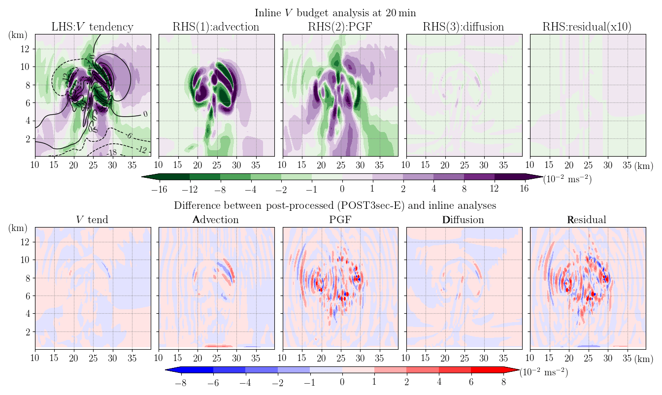
Figure 16 Upper row shows the inline budget analysis of horizontal momentum, V, for the WRF ideal test case of 2D squall line at 20 min of simulation time. Shading in subplots from left to right represents the term of V tendency, advection (ADV), horizontal pressure gradient force (PGF), diffusion, and residual (multiplied by 10 to emphasize its small magnitude as compared to the other terms). All terms are divided by μ_d and thus have units of meters per second squared. The black contours show the velocity, v, with an interval of 6 m s⁻¹. The bottom row shows the difference between the post-processed (POST3sec-E) and the inline budget analysis.

While an increase in spatial resolution often requires a shorter integration time step for numerical stability and may result in stronger simulated convection, it is almost impossible to separate all these factors. We can, however, conduct the same slantwise convection simulation with a higher resolution of 2 km (and a shorter integration time step of 10 s) to exclude the effect of different physical processes in different systems and discuss the changes in the accuracy of the budget analysis when spatial resolution is increased from 10 km. As shown in Fig. 2b, in the 2 km simulation the maximum of the simulated 99th percentile v tendency is $\mathrm{1.2}\times {\mathrm{10}}^{-\mathrm{3}}$ m s⁻², almost twice the magnitude in the 10 km run. The magnitude of the residual from the inline budget analysis also becomes larger with the 99th percentile value almost 1 order larger than that in the 10 km simulation (Fig. 5). However, its relative magnitude is still small and amounts to about 0.005 % of the tendency in the 2 km case. For the post-processed budget analysis applied to the 2 km simulation, the 99th percentile residual with the instantaneous calculation of POST10min-I-2km appears only slightly larger yet sometimes smaller than those in its 10 km case (Fig. 5a). For the method using two model outputs for both diagnosed tendency and forcing terms, the peak 99th percentile residual in POST10min-(E+I)/2-2km is about 4 times larger than that in its 10 km counterpart (POST10min-(E+I)/2). This is likely due to the larger deviation caused by the longer diagnosed window (10 min) with respect to the integration time step (10 s) in the 2 km case. In addition, it appears that the simulated fields adjust more rapidly with more complex structures on smaller scales in the 2 km simulation as compared to the 10 km simulation (not shown). If the same analysis is performed using the 1 min output (POST1min-(E+I)/2-2km) as opposed to the 10 min output, the residual can be greatly reduced to be similar to that obtained in POST10min-(E+I)/2 (Fig. 5b).

The results presented above suggest that the relative magnitude of errors in budget analysis vary with different systems or cases. Furthermore, while the absolute errors in the inline momentum budget analyses do indeed increase with increasing horizontal resolution, the relative magnitude with respect to the simulated tendency does not increase substantially. The accuracy of the post-processed budget analysis using the averages of two consecutive model outputs is highly dependent on the ratio of the output interval and the integration time step. A ratio of 10 as used in the POST10min-(E+I)/2 results in an acceptable accuracy (99th percentile residual of about 7 % of the tendency), while a lower value of 6 is required for high-resolution simulations (e.g., the 2 km case) to reach a similar accuracy. For cases with a more complex physical process like the squall line test case, the inline budget retrieval appears necessary for adequate budget closure.

5 Discussion and summary

Budget analysis is a commonly employed tool in numerical studies to understand the underlying mechanisms for certain simulated features of interest. However, many studies still have difficulties in achieving a balanced or closed budget especially when a full-physics model is used and when the budget is calculated instantaneously over a local area. Aside from the complexity of various (some implicit) parameterization schemes, the main challenge in closing the budget involves the analysis of post-processed data using algorithms that are inconsistent with the model solver. In this study, an inline momentum budget retrieval tool is developed for the WRF model, and its advantages for momentum budget analysis are demonstrated. The 99th percentile residual obtained from this inline retrieval is always smaller than or about 0.1 % of the actual tendency term in all the tested cases, which include idealized, 2D simulations of slantwise convection and squall lines. Taking the results from the inline retrieval as “truth”, we investigate the potential errors in each term and the resultant residual for post-processed budget analyses under different assumptions.

The comparison among different post-processed diagnoses is focused on the horizontal momentum (V) budget. The reason is that post-processed vertical momentum (W) budget analysis fails to produce reasonably accurate results due to the noisy vertical pressure gradient and buoyancy forces that are tied closely to the small time-step modes and the implicit scheme used for the vertical momentum integration. Thus, inline retrieval is necessary for an accurate W budget analysis. The errors in the post-processed V budget arise from both the left-hand-side tendency term and the right-hand-side (rhs) forcing terms. To improve the accuracy of the diagnosed momentum tendency estimation, one can reduce the output interval to the model integration time step, which incurs a large computational cost and consumes a large amount of disk space. An alternative and cheaper solution is to add the tendency calculation within the model as a standard output. Our test case of slantwise convection shows that the diagnosed tendency using two successive model outputs with a 10 min interval to approximate the instantaneous true tendency (with an integration time step of 1 min) could create an error exceeding 50 %, which greatly limits the effectiveness of such a budget for physical interpretation.

For the rhs forcing terms in the V equation, errors can be limited if the post-diagnosis is done with care using the same form of the model equation, the same spatial discretization, and the same order of the advection operators and performing the calculation on the original (e.g., C staggering and vertically stretched) model grids. However, these steps are necessary but not necessarily sufficient for the closure of the budget, as the forcing term diagnosis also largely depends on the selected input states. If the budget at an instant of time is desired, the explicit or forward Euler method using the previous states might result in large and widespread errors in the advection and horizontal pressure gradient terms (local peak errors are about 50 % and 25 % of their true values in our simulation, POST10min-E) unless the output interval is reduced to the integration time step. In the latter case (POST1min-E), an error <5 % for each individual term and a residual generally 1 to 2 order(s) smaller than the maximum tendency can be achieved (the 99th percentile residual is about 7 % of the 99th percentile v tendency). An alternative way to reach a similar level of accuracy for instantaneous fields without compromising the computational cost is to diagnose the rhs forcings using the implicit or backward Euler method (POST1min-I). This method diagnoses the forcings using the predicted states and thus can better capture the true model forcings by using inputs at a closer time to the model integration window.

Instead of performing the calculation using model output at one given instant, a more general post-processed budget analysis can use two successive model outputs (POST10min-(E+I)/2). This method seems to work well with the 99th percentile residual being about 7 % of the 99th percentile v tendency in our 10 km slantwise convection case with 10 min output intervals. However, the accuracy of this method varies among the test cases of different systems and is sensitive to the ratio of the output interval to the integration time step. Among the tests conducted in this study, an upper limit of 10 for this ratio is suggested, and it should be even smaller for high-resolution simulations of high-amplitude weather systems, as rapid adjustments occur on the small scales.

Three other common assumptions in post-processing analysis are made on top of the POST10min-(E+I)/2 to examine their potential impacts on the accuracy of the horizontal momentum budget analysis. First, utilizing an advection operator with a lower order than the one used in the model setup degrades the accuracy of the advection term with up to 50 % error over the area where the advection is the strongest (POST2oadv-(E+I)/2). Second, the neglect of the staggering grids would negatively impact the estimation of all the spatial differential terms, leading to a widespread residual of at least 30 % of the local tendency (POSTnonstag-(E+I)/2). Last, when the advective form of the momentum equation is used for post-diagnosis rather than the flux form, although it is mathematically equivalent to the flux form solved in the model solver, a strong negatively biased residual results (POSTadvF-(E+I)/2). Both POSTnonstag-(E+I)/2 and POSTadvF-(E+I)/2 give a peak 99th percentile residual of about >50 % of the concurrent 99th percentile of the v tendency. All the above errors do not just appear randomly; rather, they are spread over the area where the dynamics are the most active, thus undermining the physical interpretation of the dynamics of the simulated system. We thus emphasize the importance of revealing the magnitude of the residual (relative to the tendency term) in publications on budget analysis, to enable readers to gauge the validity of the results.

While the post-processed V budget analysis can reach an acceptable accuracy in some cases, the resultant residual may vary from case to case even when the same analysis method is adopted. Our test of an idealized squall line case with strong momentum tendencies shows that the application of the post-processed budget analysis method without any simplification using the 3 s (same as the model integration time step) output data nevertheless results in a large relative error magnitude (∼50 %) in the horizontal pressure gradient force, with very small-scale error structures.

In summary, different assumptions or simplifications made in a post-processed budget analysis may severely impact the estimation of each forcing term and result in a large imbalance of the budget. Based on our experiments, we conclude that the inline retrieval method like that developed herein is the most reliable one for budget analysis in numerical studies. While the budget analyses shown in this study are only for V and W momentum under the 2D idealized configurations, this newly developed budget tool also retrieves budget terms for U momentum and potential temperature. It can be applied to 3D idealized and real cases as the map projection is also considered, following the original governing equations as shown in Skamarock et al.’s (2008) Eq. (2.23)–(2.25) with map factors, which are equal to 1 for an idealized setup on the Cartesian coordinate. We also stress that in some budget studies where a coordinate transformation is necessary (e.g., from Cartesian to polar), some errors are unavoidable. In such cases, it is best to perform the budget calculation using the inline retrieval method on the model grid and then transform the budget to a new coordinate (e.g., Zhang et al., 2000). Finally, in situations where the inline coding cannot be done, this study also provides general guidance to minimize the error in the budget. Thus, our results are beneficial to budget analyses in numerical studies in general and are not limited to the WRF model.

Appendix A

To our knowledge, there are at least three other similar inline budget retrieval works that have been done in the WRF model:

1. Lehner (2012) applied to v3.2.1:

   Lehner (2012) provides a very detailed instruction of how an inline budget retrieval is done for the WRF model. The method or code was utilized in Lehner and Whiteman (2014) to study the mechanisms of the thermally driven cross-basin circulation. However, the code was never made publicly available. From the document, it appears that Lehner's (2012) general procedure of retrieving the rhs budget terms during the model integration is essentially the same as our approach, which considers both the large time-step and the small or acoustic time-step contributions. Furthermore, the individual contribution from different parameterization schemes that are activated in her study was also separately retrieved. While the general method appears highly similar to our code, the momentum budget retrieval in Lehner (2012) only applies to the horizontal momentum (U and V) whereas our tool includes the budget retrieval for the vertical momentum (W) as well.

2. Moisseeva (2014) and Moisseeva and Steyn (2014) with v3.4.1:

   The code is publicly available. The developed budget retrieval is also for the horizontal momentum equations only. The method is simpler than Lehner (2012) as it does not include the acoustic or small-step correction terms. Furthermore, while the large time-step, non-parameterized terms (e.g., pressure gradient terms, advection, Coriolis terms) are individually retrieved, their modified registry file only outputs one (summarized) term for all the parameterized physics.

3. Potter et al. (2018) with v3.8.1:

   The code is publicly available. This budget retrieval uses the code adapted from Moisseeva (2014), taking references from Lehner (2012), and is applied to the same version of the WRF model as used in this study (v3.8.1). More components are added from the version used in Moisseeva (2014), including the potential temperature budget, vertical velocity budget, the sixth-order diffusion term, the parameterized physics term decomposed to boundary layer, and radiation schemes. A major difference from our retrieval tools exists in that the small-step components are neglected in Potter et al. (2018). Comparing the budget analysis results using our retrieval tool with those using theirs for the same idealized test case of the 2D squall line, the largest differences appear in terms that involve the small-step contributions (e.g., PGF and PGFBUOY), which result in larger residual terms with Potter et al.'s (2018) retrieval method (not shown). While the relative magnitudes of such residuals to the tendency term still appear small for the horizontal momentum budget, they become larger for the vertical momentum budget. This is consistent with our result that the small-step modes are more important in the W budget equation than in the V budget equation, and thus ignoring them results in larger errors.

Furthermore, calculations of the lhs tendency terms are added as new variables in our tool while the tendency terms used in the above studies are the model variables ru_tend, rv_tend, rw_tend, etc., which only represent the summation of all the large-step forcings to their corresponding fields (can be directly outputted via changing the WRF registry file) instead of their true local changes with time.

Appendix B

To construct an initial condition that contains conditional symmetric instability (CSI) but to avoid dry symmetric instability and dry and conditional (gravitational) instability is a challenging task (Persson and Warner, 1995). Therefore, the initial profile in our test case is decided by a trial-and-error method and follows the following steps.

1. We first prescribe a horizontally uniform Brunt–Väisäilä frequency, $N^{\mathrm{2}}=\frac{g}{{\mathit{\theta }}_{\mathrm{v}}}\frac{\partial {\mathit{\theta }}_{\mathrm{v}}}{\partial z}$ with a vertical profile of

   $$\begin{array}{}\text{(B1)}& \left\{N^{\mathrm{2}}=\begin{array}{c}\mathrm{1.25}\times {\mathrm{10}}^{-\mathrm{4}}\\ \mathrm{9}\times {\mathrm{10}}^{-\mathrm{5}}\\ \mathrm{5}\times {\mathrm{10}}^{-\mathrm{4}}\end{array}{\mathrm{s}}^{-\mathrm{2}}\mathrm{for}\begin{array}{c}z<\mathrm{0.5}\mathrm{km}\\ \mathrm{5}\mathrm{km}\le z<\mathrm{10.5}\mathrm{km},\\ z\ge \mathrm{13.5}\mathrm{km}\end{array}\right.\end{array}$$

   where z is the height and there is a linear transition for the layers $\mathrm{0.5}\mathrm{km}\le z<\mathrm{5}\mathrm{km}$ and $\mathrm{10.5}\mathrm{km}\le z<\mathrm{13.5}\mathrm{km}$ using the specified values beneath and above the layers.

2. A constant geostrophic vertical zonal wind shear is given: $\frac{\partial U_{\mathrm{g}}}{\partial \mathrm{z}}=\mathrm{5.8}\times {\mathrm{10}}^{-\mathrm{3}}$ s⁻¹. Thermal wind balance gives

   $$\begin{array}{}\text{(B2)}& {\displaystyle \frac{\partial U_{\mathrm{g}}}{\partial \mathrm{z}}}=-{\displaystyle \frac{g}{f{\mathit{\theta }}_{\mathrm{v}}}}{\displaystyle \frac{\partial {\mathit{\theta }}_{\mathrm{v}}}{\partial y}}.\end{array}$$

3. Based on Eqs. (B1) and (B2), we can specify the value of θ_v at any point and then derive the θ_v for the entire domain. In this case, ${\mathit{\theta }}_{\mathrm{v}}\left(y_{\mathrm{0}},z_{\mathrm{0}}\right)=\mathrm{287.5}$ K, where (y₀,z₀) indicates the grid at the surface on the southern boundary.

4. The relative humidity (RH) field is constructed by specifying a horizontally uniform background profile (RH_background) with some enhancement (RH_bubble) over an elliptical area where the initial perturbation will be later added. The enhanced humidity over a limited area hastens the release of CSI and avoids convection developing near the southern boundary.

   $${\mathrm{RH}}_{\mathrm{background}}\left(z\right)=\left\{\begin{array}{l}\mathrm{0.81}\\ min\left[\mathrm{0.81},\mathrm{1}-\mathrm{0.9}{\left(\frac{z-\mathrm{5}}{\mathrm{7.5}}\right)}^{\mathrm{0.8}}\right]\\ \mathrm{0.1}\end{array}\right.$$
   $$\mathrm{for}\begin{array}{c}z\le \mathrm{5}\mathrm{km}\\ \mathrm{5}\mathrm{km}<z<\mathrm{12.5}\mathrm{km}\\ z\ge \mathrm{12.5}\mathrm{km}\end{array},$$
   $${\mathrm{RH}}_{\mathrm{bubble}}\left(y,z\right)={\mathrm{RH}}_{\mathrm{background}}\left(z\right)\times f_{\mathrm{enhancement}}\left(y,z\right),$$

   where

   $$\begin{array}{rl}& f_{\mathrm{enhancement}}\left(y,z\right)=\\ & \left\{\begin{array}{l}\mathrm{1.22}\\ \mathrm{1.22}-\mathrm{0.11}\left(e-\mathrm{1}\right)\\ \mathrm{1}\end{array}\right.\mathrm{for}\begin{array}{c}e\le \mathrm{1}\\ \mathrm{1}<e\le \mathrm{3}\\ e>\mathrm{3}\end{array},\end{array}$$

   where $e={\left(\frac{y-\mathrm{410}}{e_{\mathrm{b}}}\right)}^{\mathrm{2}}+{\left(\frac{z-\mathrm{1}}{e_{\mathrm{a}}}\right)}^{\mathrm{2}}$, $e_{\mathrm{b}}=\mathrm{100},e_{\mathrm{a}}=\mathrm{3}$, and y and z are the horizontal distance from the southern boundary and height, respectively, with units of kilometers. The constructed initial profile has a maximum RH of 98.82 % over an elliptical area centered at y=410 km and z=1 km.

5. A constant surface pressure is specified: p_sfc=1000 hPa.

6. We then iteratively solve for the hydrostatically balanced pressure, water vapor mixing ratio, potential temperature, dry and full (moist) air density, and geostrophic zonal wind for the entire domain.

The constructed initial environment contains some CSI, which is identified by the presence of negative saturated geostrophic potential vorticity (Chen et al., 2018). In this test case, CSI only exists over the southern half of the domain and never extends higher than 5 km.

To initiate convection, a 2D bubble of potential temperature and zonal wind perturbations is inserted in the area where RH is maximized and where the saturated geostrophic potential vorticity has a value of about $-\mathrm{0.2}\sim -\mathrm{0.1}$ pvu. The center of the bubble, located at y_c=400 km and z_c=1.5 km, has a maximum potential temperature perturbation Δθ_max=0.5 K and zonal wind perturbation $\mathrm{\Delta }{u}_{\max }=-\mathrm{6}$ m s⁻¹. Both perturbation fields decrease to 0 with radius, following Δθ=Δθ_maxcos²(0.5πr) and Δu=Δu_maxcos²(0.5πr), for $r<=\mathrm{1}$, where $r=\sqrt{(\frac{y-y_{\mathrm{c}}}{R}{)}^{\mathrm{2}}+(\frac{z-z_{\mathrm{c}}}{H}{)}^{\mathrm{2}}}$, R=50 km is the horizontal radius, and H=1.5 km is the vertical radius.