the Creative Commons Attribution 4.0 License.
the Creative Commons Attribution 4.0 License.
 | 01 Apr 2020
Statistical downscaling with the downscaleR package (v3.1.0): contribution to the VALUE intercomparison experiment
Jorge Baño-Medina
Mikel N. Legasa
Maialen Iturbide
Rodrigo Manzanas
Sixto Herrera
Ana Casanueva
Daniel San-Martín
Antonio S. Cofiño
José Manuel Gutiérrez
The increasing demand for high-resolution climate information has attracted growing attention to statistical downscaling (SDS) methods, due in part to their relative advantages and merits as compared to dynamical approaches (based on regional climate model simulations), such as their much lower computational cost and their fitness for purpose for many local-scale applications. As a result, a plethora of SDS methods is nowadays available to climate scientists, which has motivated recent efforts for their comprehensive evaluation, like the VALUE initiative (http://www.value-cost.eu, last access: 29 March 2020). The systematic intercomparison of a large number of SDS techniques undertaken in VALUE, many of them independently developed by different authors and modeling centers in a variety of languages/environments, has shown a compelling need for new tools allowing for their application within an integrated framework. In this regard, downscaleR is an R package for statistical downscaling of climate information which covers the most popular approaches (model output statistics – including the so-called “bias correction” methods – and perfect prognosis) and state-of-the-art techniques. It has been conceived to work primarily with daily data and can be used in the framework of both seasonal forecasting and climate change studies. Its full integration within the climate4R framework (Iturbide et al., 2019) makes possible the development of end-to-end downscaling applications, from data retrieval to model building, validation, and prediction, bringing to climate scientists and practitioners a unique comprehensive framework for SDS model development.
In this article the main features of downscaleR are showcased through the replication of some of the results obtained in VALUE, placing an emphasis on the most technically complex stages of perfect-prognosis model calibration (predictor screening, cross-validation, and model selection) that are accomplished through simple commands allowing for extremely flexible model tuning, tailored to the needs of users requiring an easy interface for different levels of experimental complexity. As part of the open-source climate4R framework, downscaleR is freely available and the necessary data and R scripts to fully replicate the experiments included in this paper are also provided as a companion notebook.
- Article
(4348 KB) - Full-text XML
- BibTeX
- EndNote


Global climate models (GCMs) – atmospheric, coupled oceanic–atmospheric, and earth system models – are the primary tools used to generate weather and climate predictions at different forecast horizons, from intra-seasonal to centennial scales. However, raw model outputs are often not suitable for climate impact studies due to their limited resolution (typically hundreds of kilometers) and the presence of biases in the representation of regional climate (Christensen et al., 2008), attributed to a number of reasons such as the imperfect representation of physical processes and the coarse spatial resolution that does not permit an accurate representation of small-scale processes. To partially overcome these limitations, a wide variety of downscaling techniques have been developed, aimed at bridging the gap between the coarse-scale information provided by GCMs and the regional or local climate information required for climate impact and vulnerability analysis. To this aim both dynamical (based on regional climate models, RCMs; see, e.g., Laprise, 2008) and empirical or statistical approaches have been introduced during the last decades. In essence, statistical downscaling (SDS; Maraun and Widmann, 2018) methods rely on the establishment of a statistical link between the local-scale meteorological series (predictand) and large-scale atmospheric variables at different pressure levels (predictors, e.g., geopotential, temperature, humidity). The statistical models or algorithms used in this approach are first calibrated using historical (observed) data of both coarse predictors (reanalysis) and local predictands for a representative climatic period (usually a few decades) and then applied to new (e.g., future or retrospective) global predictors (GCM outputs) to obtain the corresponding locally downscaled predictands (von Storch et al., 1993). SDS techniques were first applied in short-range weather forecast (Klein et al., 1959; Glahn and Lowry, 1972) and later adapted to larger prediction horizons, including seasonal forecasts and climate change projections, the latter the problem being the one that has received the most extensive attention in the literature. SDS techniques are often also applied to RCM outputs (usually referred to as “hybrid downscaling”, e.g., Turco and Gutiérrez, 2011), and therefore both approaches (dynamical and statistical) can be regarded as complementary rather than mutually exclusive .
Notable efforts have been made in order to assess the credibility of regional climate change scenarios. In the particular case of SDS, a plethora of methods exists nowadays, and a thorough assessment of their intrinsic merits and limitations is required to guide practitioners and decision makers with credible climate information (Barsugli et al., 2013). In response to this challenge, the COST Action VALUE (Maraun et al., 2015) is an open collaboration that has established a European network to develop and validate downscaling methods, fostering collaboration and knowledge exchange between dispersed research communities and groups, with the engagement of relevant stakeholders (Rössler et al., 2019). VALUE has undertaken a comprehensive validation and intercomparison of a wide range of SDS methods (over 50), representative of the most common techniques covering the three main approaches, namely perfect prognosis, model output statistics – including bias correction – and weather generators (Gutiérrez et al., 2019). VALUE also provides a common experimental framework for statistical downscaling and has developed community-oriented validation tools specifically tailored to the systematic validation of different quality aspects that had so far received little attention (see Maraun et al., 2019b, for an overview), such as the ability of the downscaling predictions to reproduce the observed temporal variability (Maraun et al., 2019a), the spatial variability among different locations (Widmann et al., 2019), reproducibility of extremes (Hertig et al., 2019), and process-based validation (Soares et al., 2019).
The increasing demand for high-resolution predictions or projections for climate impact studies and the relatively fast development of SDS in the last decades, with a growing number of algorithms and techniques available, has motivated the development of tools for bridging the gap between the inherent complexities of SDS and the user's needs, able to provide end-to-end solutions in order to link the outputs of the GCMs and ensemble prediction systems to a range of impact applications. One pioneer service was the interactive, web-based Downscaling Portal (Gutiérrez et al., 2012) developed within the EU-funded ENSEMBLES project (van der Linden and Mitchell, 2009), integrating the necessary tools and providing the appropriate technology for distributed data access and computing and enabling user-friendly development and evaluation of complex SDS experiments for a wide range of alternative methods (analogs, weather typing, regression, etc.). The Downscaling Portal is in turn internally driven by MeteoLab, (https://meteo.unican.es/trac/MLToolbox/wiki), an open-source Matlab™ toolbox for statistical analysis and data mining in meteorology, focused on statistical downscaling methods.
There are other existing tools available to the R computing environment implementing SDS methods (beyond the most basic model output statistics (MOS) and “bias correction” techniques not addressed in this study, but see Sect. 2), like the R package esd (Benestad et al., 2015), freely available from the Norwegian Meteorological Institute (MET Norway). This package provides utilities for data retrieval and manipulation, statistical downscaling, and visualization, implementing several classical methods (EOF analysis, regression, canonical correlation analysis, multivariate regression, and weather generators, among others). A more specific downscaling tool is provided by the package Rglimclim (https://www.ucl.ac.uk/~ucakarc/work/glimclim.html, last access: 29 March 2020), a multivariate weather generator based on generalized linear models (see Sect. 2.2) focused on model fitting and simulation of multisite daily climate sequences, including the implementation of graphical procedures for examining fitted models and simulation performance (see, e.g., Chandler and Wheater, 2002).
More recently, the climate4R framework (Iturbide et al., 2019), based on the popular R language (R Core Team, 2019) and other external open-source software components (NetCDF-Java, THREDDS, etc.), has also contributed with a variety of methods and advanced tools for climate impact applications, including statistical downscaling. climate4R is formed by different seamlessly integrated packages for climate data access, processing (e.g., collocation, binding, and subsetting), analysis, and visualization, tailored to the needs of the climate impact assessment communities in various sectors and applications, including comprehensive metadata and output traceability (Bedia et al., 2019a), and provided with extensive documentation, wiki pages, and worked examples (notebooks) allowing reproducibility of several research papers (see, e.g., https://github.com/SantanderMetGroup/notebooks, last access: 29 March 2020). Furthermore, the climate4R Hub is a cloud-based computing facility that allows users to run climate4R on the cloud using docker and a Jupyter Notebook (https://github.com/SantanderMetGroup/climate4R/tree/master/docker, last access: 29 March 2020). The climate4R framework is presented by Iturbide et al. (2019), and some of its specific components for sectoral applications are illustrated, e.g., in Cofiño et al. (2018) (seasonal forecasting), Frías et al. (2018) (visualization), Bedia et al. (2018) (forest fires), or Iturbide et al. (2018) (species distributions). In this context, the R package downscaleR has been conceived as a new component of climate4R to undertake SDS exercises, allowing for a straightforward application of a wide range of methods. It builds on the previous experience of the MeteoLab Toolbox in the design and implementation of advanced climate analysis tools and incorporates novel methods and enhanced functionalities implementing the state-of-the-art SDS techniques to be used in forthcoming intercomparison experiments in the framework of the EURO-CORDEX initiative (Jacob et al., 2014), in which the VALUE activities have merged and will follow on. As a result, unlike previous existing SDS tools available in R, downscaleR is integrated within a larger climate processing framework providing end-to-end solutions for the climate impact community, including efficient access to a wide range of data formats, either remote or locally stored, extensive data manipulation and analysis capabilities, and export options to common geoscientific file formats (such as netCDF), thus providing maximum interoperability to accomplish successful SDS exercises in different disciplines and applications.
This paper introduces the main features of downscaleR for perfect-prognosis statistical downscaling (as introduced in Sect. 2) using to this aim some of the methods contributing to VALUE. The particular aspects related to data preprocessing (predictor handling, etc.), SDS model configuration, and downscaling from GCM predictors are described, thus covering the whole downscaling cycle from the user's perspective. In order to showcase the main downscaleR capabilities and its framing within the ecosystem of applications brought by climate4R, the paper reproduces some of the results of the VALUE intercomparison presented by Gutiérrez et al. (2019), using public datasets (described in Sect. 3.1) and considering two popular SDS techniques (analogs and generalized linear models), described in Sect. 2.2. The downscaleR functions and the most relevant parameters used in each experiment are shown in Sects. 3.3 and 4, after a schematic overview of the different stages involved in a typical perfect-prognosis SDS experiment (Sect. 2.1). Finally in Sect. 4.2, locally downscaled projections of precipitation for a high-emission scenario (RCP 8.5) are calculated for the future period 2071–2100 using the output from one state-of-the-art GCM contributing to the CMIP5.
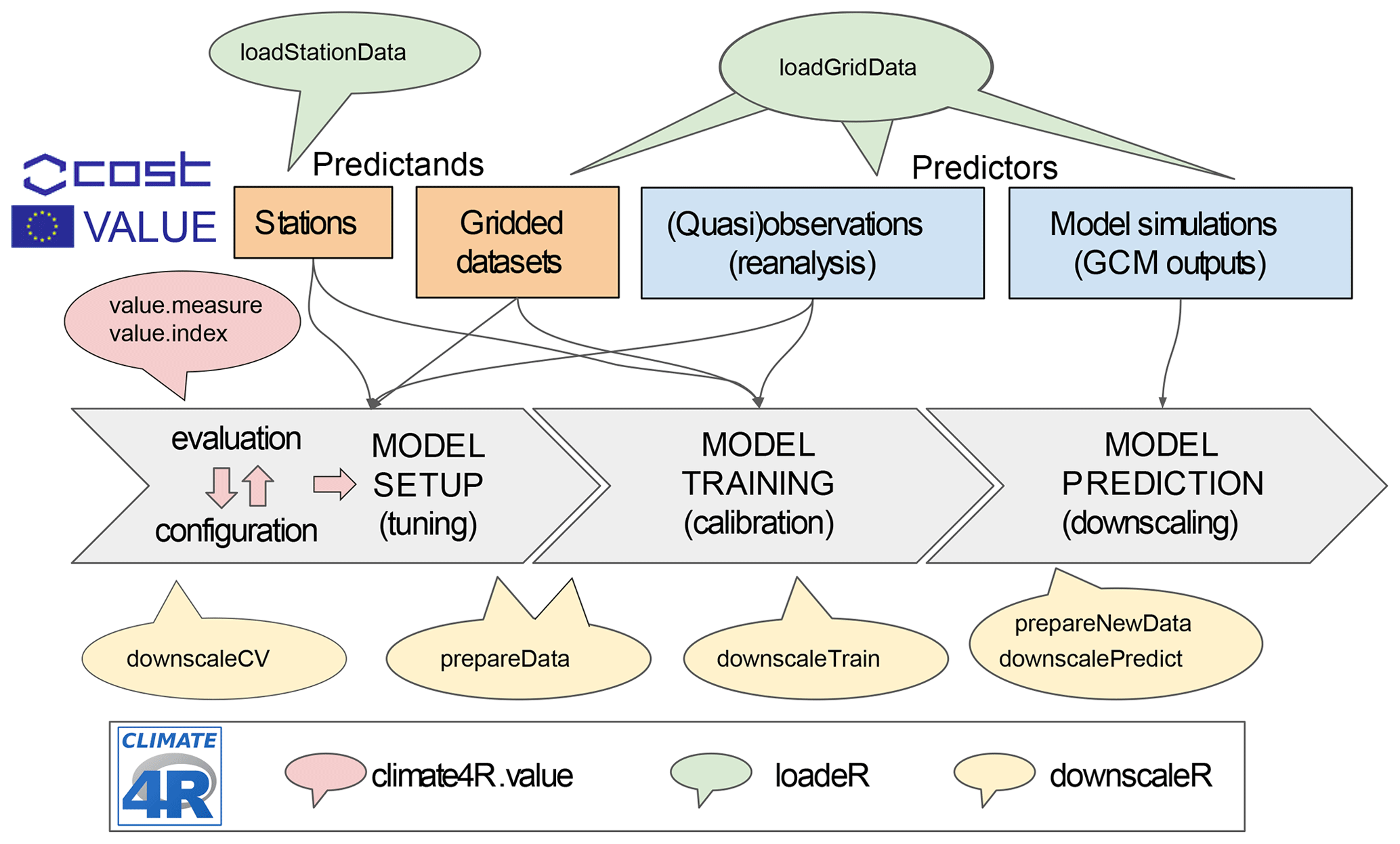
Figure 1Schematic overview of the R package downscaleR and its framing into the climate4R framework for climate data access and analysis. The typical perfect-prognosis downscaling phases are indicated by the gray arrows. (i) In the first place, model setup is undertaken. This process is iterative and usually requires testing many different model configurations under a cross-validation setup until an optimal configuration is achieved. The downscaleCV function (and prepareData under the hood) is used in this stage for a fine-tuning of the model. Model selection is determined through the use of indices and measures reflecting model suitability for different aspects that usually depend on specific research aims (e.g., good reproducibility of extreme events, temporal variability, spatial dependency across different locations). The validation is achieved through the climate4R.value package (red-shaded callout), implementing the VALUE validation framework. (ii) Model training: once an optimal model is achieved, model training is performed using the downscaleTrain function. (iii) Finally, the calibrated model is used to undertake downscaling (i.e., model predictions) using the function downscalePredict. The data to be used in the predictions requires appropriate preprocessing (e.g., centering and scaling using the predictor set as reference, projection of PCs onto predictor EOFs) that is performed under the hood by the function prepareNewData prior to model prediction with downscalePredict.
downscaleR The application of SDS techniques to the global outputs of a GCM (or RCM) typically entails two phases. In the training phase, the model parameters (or algorithms) are fitted to data (or tuned or calibrated) and cross-validated using a representative historical period (typically a few decades) with existing predictor and predictand data. In the downscaling phase, which is common to all SDS methods, the predictors given by the GCM outputs are plugged into the models (or algorithms) to obtain the corresponding locally downscaled values for the predictands. According to the approach followed in the training phase, the different SDS techniques can be broadly classified into two categories (Rummukainen, 1997; Marzban et al., 2006; also see Maraun and Widmann, 2018, for a discussion on these approaches), namely perfect prognosis (PP) and MOS. In the PP approach, the statistical model is calibrated using observational data for both the predictands and predictors (see, e.g., Charles et al., 1999; Timbal et al., 2003; Bürger and Chen, 2005; Haylock et al., 2006; Fowler et al., 2007; Hertig and Jacobeit, 2008; Sauter and Venema, 2011; Gutiérrez et al., 2013). In this case, “observational” data for the predictors are taken from a reanalysis (which assimilates day by day the available observations into the model space). In general, reanalyses are more constrained by assimilated observations than by internal model variability and thus can reasonably be assumed to reflect “reality” (Sterl, 2004). The term “perfect” in PP refers to the assumption that the predictors are bias-free. This assumption is generally accepted (although it may not hold true in the tropics; see, e.g., Brands et al., 2012). As a result, in the PP approach predictors and predictand preserve day-to-day correspondence. Unlike PP, in the MOS approach the predictors are taken from the same GCM (or RCM) for both the training and downscaling phases. For instance, in MOS approaches, local precipitation is typically downscaled from the direct model precipitation simulations (Widmann et al., 2003). In weather forecasting applications MOS techniques also preserve the day-to-day correspondence between predictors and predictand, but, unlike PP, this does not hold true in a climate context. As a result, MOS methods typically work with the (locally interpolated) predictions and observations of the variable of interest (a single predictor). In MOS, the limitation of having homogeneous predictor–predictand relationships applies only in a climate context, and therefore many popular bias correction techniques (e.g., linear scaling, quantile–quantile mapping) lie in this category. In this case, the focus is on the statistical similarity between predictor and predictand, and there is no day-to-day correspondence of both series during the calibration phase. The application of MOS techniques in a climate context using downscaleR is already shown in Iturbide et al. (2019). Here, the focus is on the implementation of PP methods that entail greater technical complexities for their application from a user's perspective but have received less attention from the side of climate service development. A schematic diagram showing the main phases of perfect-prognosis downscaling is shown in Fig. 1.
2.1 SDS model setup: configuration of predictors
As general recommendations, a number of aspects need to be carefully addressed when looking for suitable predictors in the PP approach (Wilby et al., 2004; Hanssen-Bauer et al., 2005): (i) the predictors should account for a major part of the variability in the predictands, (ii) the links between predictors and predictands should be temporally stable or stationary, and (iii) the large-scale predictors must be realistically reproduced by the global climate model. Since different global models are used in the calibration and downscaling phases, large-scale circulation variables well represented by the global models are typically chosen as predictors in the PP approach, whereas variables directly influenced by model parametrizations and/or orography (e.g., precipitation) are usually not considered. For instance, predictors generally fulfilling these conditions for downscaling precipitation are humidity, geopotential, or air temperature (see Sect. 3.1.2) at different surface pressure vertical levels. Only sea-level pressure and 2 m air temperature are usually used as near-surface predictors. An example of the evaluation of this hypothesis is later presented in Sect. 4.2.1 of this study. Often, predictors are proxies for physical processes, which is a main reason for non-stationarities in the predictor–predictand relationship, as amply discussed in Maraun and Widmann (2018). Furthermore, reanalysis choice has been reported as an additional source of uncertainty for SDS model development (Brands et al., 2012), although its effect is of relevance only in the tropics (see, e.g., Manzanas et al., 2015). With regard to the assumption (ii), predictor selection and the training of transfer functions are carried out on short-term variability in present climate, whereas the aim is typically to simulate long-term changes in short-term variability (Huth, 2004; Maraun and Widmann, 2018), which limits the performance of PP and makes it particularly sensitive to the method type and the predictor choice (Maraun et al., 2019b).
For all these reasons, the selection of informative and robust predictors during the calibration stage is a crucial step in SDS modeling (Fig. 1), model predictions being very sensitive to the strategy used for predictor configuration (see, e.g., Benestad, 2007; Gutiérrez et al., 2013). PP techniques can consider point-wise and/or spatial-wise predictors, using either the raw values of a variable over a region of a user-defined extent or only at nearby grid boxes and/or the principal components (PCs) corresponding to the empirical orthogonal functions (EOFs; Preisendorfer, 1988) of the variables considered over a representative geographical domain (which must be also conveniently determined). Usually, the latter are more informative in those cases where the local climate is mostly determined by synoptic phenomena, whereas the former may be needed to add some information about the local variability in those cases where small-scale processes are important (see, e.g., Benestad, 2001). Sometimes, both types of predictors are combined in order to account for both synoptic and local effects. In this sense, three non-mutually exclusive options are typically used in the downscaling experiments next summarized:
-
using raw atmospheric fields for a given spatial domain, typically continental- or nation-wide for downscaling monthly and daily data, respectively. For instance, in the VALUE experiment, predefined subregions within Europe are used for training (Fig. 2), thus helping to reduce the dimension of the predictor set. Alternatively, stepwise or regularized methods can be used to automatically select the predictor set from the full spatial domain.
-
using principal components obtained from these fields (Benestad, 2001). Working with PCs allows users to filter out high-frequency variability which may not be properly linked to the local scale, greatly reducing the dimensionality of the problem related to the deletion of redundant and/or collinear information from the raw predictors. These predictors convey large-scale information to the predictor set and are often also referred to as “spatial predictors”. These can be a number of principal components calculated upon each particular variable (e.g., explaining 95 % of the variability) and/or a combined PC calculated upon the (joined) standardized predictor fields (“combined” PCs).
-
The spatial extent of each predictor field may have a strong effect on the resulting model. Some variables of the predictor set may have explanatory power only nearby the predictand locations, while the useful information is diluted when considering larger spatial domains. As a result, it is common practice to include local information in the predictor set by considering only a few grid points around the predictand location for some of the predictor variables (this can be just the closest grid point or a window of a user-defined width). This category can be regarded as a particular case of point 1 but considering a much narrower window centered around the predictand location. This local information is combined with the “global” information provided by other global predictors (either raw fields – case 1 – or principal components – case 2) encompassing a larger spatial domain.
Therefore, predictor screening (i.e., variable selection) and their configuration is one of the most time-consuming tasks in perfect-prognosis experiments due to the potentially huge number of options required for a fine-tuning of the predictor set (spatial, local, or a combination of both, number of principal components, and methodology for their generation, etc.). As a result, SDS model tuning is iterative and usually requires testing many different model configurations until an optimal one is attained (see, e.g., Gutiérrez et al., 2013), as next described in Sect. 2.3. This requires a flexible yet easily configurable interface, enabling users to launch complex experiments for testing different predictor setups in a straightforward manner. In downscaleR, the function prepareData has been designed to this aim, providing maximum user flexibility for the definition of all types of predictor configurations with a single command call, building upon the raw predictor information (see Sect. 3.3).
2.2 Description of SDS methods
downscaleR implements several PP techniques, ranging from the classical analogs and regression to more recent and sophisticated machine-learning methods (Baño-Medina et al., 2019). For brevity, in this study we focus on the standard approaches contributing to the VALUE intercomparison, namely analogs, linear models, and generalized linear models, next briefly introduced; the up-to-date description of methods is available at the downscaleR wiki (https://github.com/SantanderMetGroup/downscaleR/wiki, last access: 29 March 2020). All the SDS methods implemented in downscaleR are applied using unique workhorse functions, such as downscaleCV (cross-validation), downscaleTrain (for model training), and downscalePredict (for model prediction) (Fig. 1), that receive the different tuning parameters for each method chosen, providing maximum user flexibility for the definition and calibration of the methods. Their application will be illustrated throughout Sects. 3.3 and 4.
2.2.1 Analogs
This is a non-parametric analog technique (Lorenz, 1969; Zorita and von Storch, 1999), based on the assumption that similar (or analog) atmospheric patterns (predictors) over a given region lead to similar local meteorological outcomes (predictand). For a given atmospheric pattern, the corresponding local prediction is estimated according to a determined similarity measure (typically the Euclidean norm, which has been shown to perform satisfactorily in most cases; see, e.g., Matulla et al., 2008) from a set of analog patterns within a historical catalog over a representative climatological period. In PP, this catalog is formed by reanalysis data. In spite of its simplicity, analog performance is competitive against other more sophisticated techniques (Zorita and von Storch, 1999), being able to take into account the non-linearity of the relationships between predictors and predictands. Additionally, it is spatially coherent by construction, preserving the spatial covariance structure of the local predictands as long as the same sequence of analogs for different locations is used, spatial coherence being underestimated otherwise (Widmann et al., 2019). Hence, analog-based methods have been applied in several studies both in the context of climate change (see, e.g., Gutiérrez et al., 2013) and seasonal forecasting (Manzanas et al., 2017). The main drawback of the analog technique is that it cannot predict values outside the observed range, therefore being particularly sensitive to the non-stationarities arising in climate change conditions (Benestad, 2010) and thus preventing its application to the far future, when temperature and directly related variables are considered (see, e.g., Bedia et al., 2013).
2.2.2 Linear models (LMs)
(Multiple) linear regression is the most popular downscaling technique for suitable variables (e.g., temperature), although it has been also applied to other variables after suitable transformation (e.g., to precipitation, typically taking the cubic root). Several implementations have been proposed including spatial (PC) and/or local predictors. Moreover, automatic predictor selection approaches (e.g., stepwise) have been also applied (see Gutiérrez et al., 2019, for a review).
2.2.3 Generalized linear models (GLMs)
They were formulated by Nelder and Wedderburn (1972) in the 1970s and are an extension of the classical linear regression, which allows users to model the expected value of a random predictand variable whose distribution belongs to the exponential family (Y) through an arbitrary mathematical function called link function (g) and a set of unknown parameters (β), according to
where X is the predictor and E(Y) the expected value of the predictand. The unknown parameters, β, can be estimated by maximum likelihood, considering a least-squares iterative algorithm.
GLMs have been extensively used for SDS in climate change applications (e.g., Brandsma and Buishand, 1997; Chandler and Wheater, 2002; Abaurrea and Asín, 2005; Fealy and Sweeney, 2007; Hertig et al., 2013) and, more recently, also for seasonal forecasts (Manzanas et al., 2017). For the case of precipitation, a two-stage implementation (see, e.g., Chandler and Wheater, 2002) must be used given its dual (occurrence–amount) character. In this implementation, a GLM with Bernoulli error distribution and logit canonical link function (also known as logistic regression) is used to downscale precipitation occurrence (0= no rain; 1= rain) and a GLM with gamma error distribution and log canonical link function is used to downscale precipitation amount, considering wet days only. After model calibration, new daily predictions are given by simulating from a gamma distribution, whose shape parameter is fitted using the observed wet days in the calibration period.
Beyond the classical GLM configurations, downscaleR allows using both deterministic and stochastic versions of GLMs. In the former, the predictions are obtained from the expected values estimated by both the GLM for occurrence (GLMo) and the GLM for amount (GLMa). In the GLMo, the continuous expected values are transformed into binary ones as 1 (0) either by fixing a cutoff probability value (e.g., 0.5) or by choosing a threshold based on the observed predictand climatology for the calibration period (the latter is the default behavior in downscaleR). By contrast, for GLMa, the expected values are directly interpreted as rain amounts. Moreover, downscaleR gives the option of generating stochastic predictions for both the GLMo the and GLMa, which could be seen as a dynamic predictor-driven version of the inflation of variance used in some regression-based methods (Huth, 1999).
2.3 SDS model validation
When assessing the performance of any SDS technique it is crucial to properly cross-validate the results in order to avoid misleading conclusions about model performance due to artificial skill. This is typically achieved considering a historical period for which observations exist to validate against. k-fold and leave-one-out cross-validation are among the most widely applied validation procedures in SDS experiments. In a k-fold cross-validation framework (Stone, 1974; Markatou et al., 2005), the original sample (historical period) is partitioned into k equally sized and mutually exclusive subsamples (folds). In each of the k iterations, one of these folds is retained for testing (prediction phase) and the remaining k−1 folds are used for training (calibration phase). The resulting k independent samples are then merged to produce a single time series covering the whole calibration period, which is subsequently validated against observations. When k=n (being n the number of observations), the k-fold cross-validation is exactly the leave-one-out cross-validation (Lachenbruch and Mickey, 1968). Another common approach is the simpler “holdout” method, that partitions the data into just two mutually exclusive subsets (k=2), called the training and test (or holdout) sets. In this case, it is common to designate two-thirds of the data as the training set and the remaining one-third as the test set (see, e.g., Kohavi, 1995).
Therefore, PP models are first cross-validated under “perfect conditions” (i.e., using reanalysis predictors) in order to evaluate their performance against real historical climate records before being applied to “non-perfect” GCM predictors. Therefore, the aim of cross-validation in the PP approach is to properly estimate, given a known predictor dataset (large-scale variables from reanalysis), the performance of the particular technique considered, having an “upper bound” for its generalization capability when applied to new predictor data (large-scale variables from GCM). The workhorse for cross-validation in downscaleR is the function downscaleCV, which adequately handles data partition to create the training and test data subsets according to the parameters specified by the user, being tailored to the special needs of statistical downscaling experiments (i.e., random temporal or spatial folds, leave-one-year-out, arbitrary selection of years as folds, etc.).
During the cross-validation process, one or several user-defined measures are used in order to assess model performance (i.e., to evaluate how “well” do model predictions match the observations), such as accuracy measures, distributional similarity scores, inter-annual variability, and trend matching scores. In this sense, model quality evaluation is a multi-faceted task with many possible and often unrelated aspects to look into. Thus, validation ultimately consists of deriving specific climate indices from model output, comparing these indices to reference indices calculated from observational data and quantifying the mismatch with the help of suitable performance measures (Maraun et al., 2015). In VALUE, the term “index” is used in a general way, including not only single numbers (e.g., the 90th percentile of precipitation, lag-1 autocorrelation) but also vectors such as time series (for instance, a binary time series of rain or no rain). Specific “measures” are then computed upon the predicted and observed indices, for instance the difference (bias, predicted – observed) of numeric indices or the correlation of time series (Sect. 3.3.9). A comprehensive list of indices and measures has been elaborated by the VALUE cross-cutting group in order to undertake a systematic evaluation of downscaling methods. The complete list is presented in the VALUE Validation Portal (http://www.value-cost.eu/validationportal/app/#!indices, last access: 29 March 2020). Furthermore, all the VALUE indices and measures have been implemented in R and collected in the package VALUE (https://github.com/SantanderMetGroup/VALUE, last access: 29 March 2020), allowing for further collaboration and extension with other initiatives, as well as for research reproducibility. The validation tools available in VALUE have been adapted to the specific data structures of the climate4R framework (see Sect. 1) through the wrapping package climate4R.value (https://github.com/SantanderMetGroup/climate4R.value, last access: 29 March 2020), enabling a direct application of the comprehensive VALUE validation framework to downscaling exercises with downscaleR (Fig. 1). A summary of the subset of VALUE indices and measures used in this study is presented in Table 1.
Table 1Summary of the subset of VALUE validation indices and measures used in this study. Their codes are consistent with the VALUE reference list (http://www.value-cost.eu/validationportal/app/#!indices), except for “ts.ks.pval”, which has been included later in the VALUE set of measures.
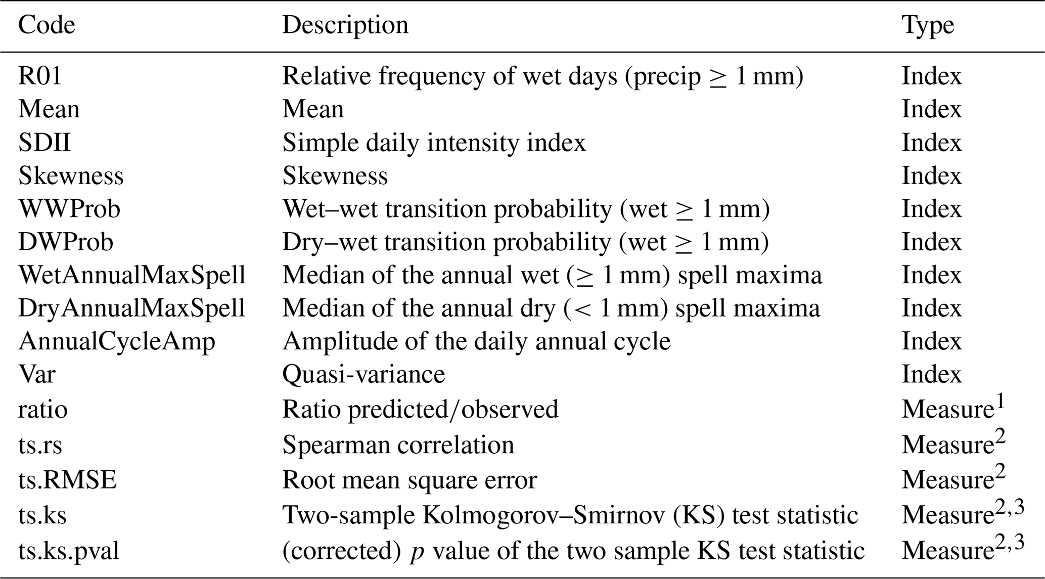
The superscripts in the measures indicate the input used to compute them: 1 – a single scalar value, corresponding to the predicted and observed indices; 2 – the original predicted and observed precipitation time series; 3 – transformed time series (centered anomalies or standardized anomalies).
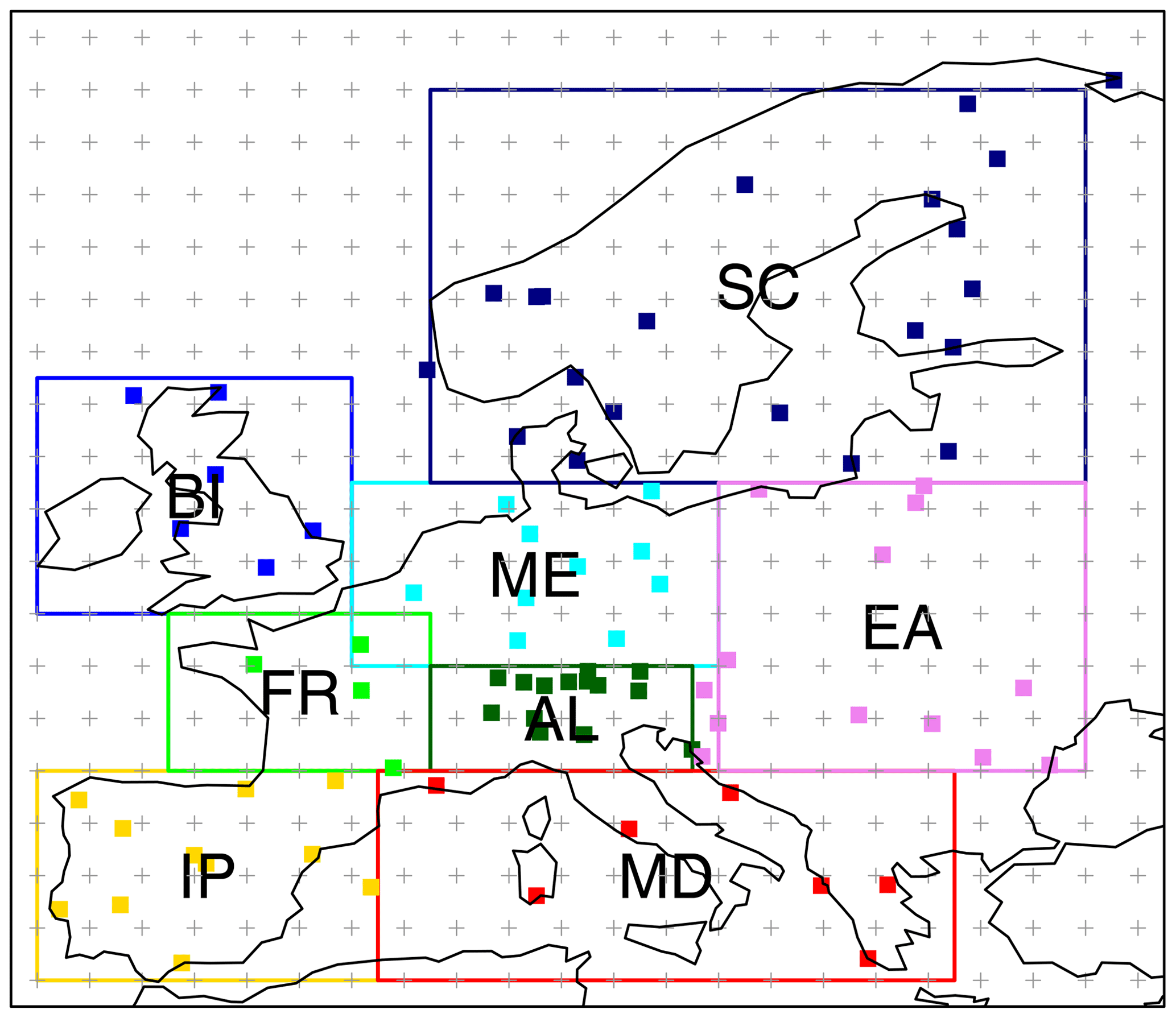
Figure 2Location of the 86 stations of the ECA-VALUE-86 dataset (red squares). The colored boxes show the eight PRUDENCE subregions considered in the VALUE downscaling experiment for model training (Sect. 3.1). The regular grid of the predictor dataset, a 2∘×2∘ resolution version of the ERA-Interim reanalysis, is also shown. The subregions considered are IP (Iberian Peninsula), FR (France), BI (British Isles), MD (Mediterranean), AL (Alps), ME (central Europe), SC (Scandinavia), and EA (eastern Europe). Station metadata can be interactively queried through the VALUE Validation Portal application (http://www.value-cost.eu/validationportal/app/#!datasets, last access: 29 March 2020).
The VALUE initiative (Maraun et al., 2015) produced the largest-to-date intercomparison of statistical downscaling methods with over 50 contributing techniques. The contribution of MeteoLab (and downscaleR) to this experiment included a number of methods which are fully reproducible with downscaleR, as we show in this example. This pan-European contribution was based on previous experience over the Iberian domain (Gutiérrez et al., 2013; San-Martín et al., 2016), testing a number of predictor combinations and method configurations. In order to illustrate the application of downscaleR, in this example we first revisit the experiment over Iberian domain (but considering the VALUE framework and data), showing the code undertaking the different steps (Sect. 3.3). Afterwards, the subset of methods contributing to VALUE is applied at a pan-European scale, including also results of future climate scenarios (Sect. 4).
In order to reproduce the results of the VALUE intercomparison, the VALUE datasets are used in this study (Sect. 3.1). In addition, future projections from a CMIP5 GCM are also used to illustrate the application of the downscaling methods to climate change studies. For transparency and full reproducibility, the datasets are public and freely available for download using the climate4R tools, as indicated in Sect. 3.2. Next, the datasets are briefly presented. Further information on the VALUE data characteristics is given in Maraun et al. (2015) and Gutiérrez et al. (2019) and also at their official download URL (http://www.value-cost.eu/data, last access: 29 March 2020). The reference period considered for model evaluation in perfect conditions is 1979–2008. In the analysis of the GCM predictors (Sect. 4.2.1), this period is adjusted to 1979–2005 constrained by the period of the historical experiment of the CMIP5 models (Sect. 3.1.3). The future period for presenting the climate change signal analysis is 2071–2100.
3.1 Datasets
3.1.1 Predictand data (weather station records)
The European station dataset used in VALUE has been carefully prepared in order to be representative of the different European climates and regions and with a reasonably homogeneous spatial density (Fig. 2). To keep the exercise as open as possible, the downloadable (blended) ECA&D stations (Klein Tank et al., 2002) were used. From this, a final subset of 86 stations was selected with the help of local experts in the different countries, restricted to high-quality stations with no more than 5 % of missing values in the analysis period (1979–2008). Further details on predictand data preprocessing are provided in http://www.value-cost.eu/WG2_dailystations (last access: 29 March 2020). The full list of stations is provided in Table 1 in Gutiérrez et al. (2019).
3.1.2 Predictor data (reanalysis)
In line with the experimental protocol of the Coordinated Regional Climate Downscaling Experiment (CORDEX; Giorgi et al., 2009), VALUE has used ERA-Interim (Dee et al., 2011) as the reference reanalysis to drive the experiment with perfect predictors. For full comparability, the list of predictors used in VALUE is replicated in this study – see Table 2 in Gutiérrez et al. (2019) – namely sea-level pressure, 2 m air temperature, air temperature and relative humidity at 500, 700, and 850 hPa surface pressure levels, and the geopotential height at 500 hPa.
The set of raw predictors corresponds to the full European domain shown in Fig. 2. The eight reference regions defined in the PRUDENCE project of model evaluation (Christensen et al., 2007) were used in VALUE as appropriate regional domains for training the models of the corresponding stations (Sect. 2.1). The stations falling within each domain are colored accordingly in Fig. 2.
3.1.3 Predictor data (GCM future projections)
In order to illustrate the application of SDS methods to downscale future global projections from GCM predictors, here we consider the outputs from the EC-EARTH model (in particular the r12i1p1 ensemble member; EC-Earth Consortium, 2014) for the 2071–2100 period under the RCP8.5 scenario (Moss et al., 2010). This simulation is part of CMIP5 (Taylor et al., 2011) and is officially served by the Earth System Grid Federation infrastructure (ESGF; Cinquini et al., 2014). In this study, data are retrieved from the Santander User Data Gateway (Sect. 4.2), which is the data access layer of the climate4R framework (described in Sect. 3.2).
Table 2Summary of predictor configurations tested. Local predictors always correspond to the original predictor fields previously standardized. Independent PCs are calculated separately for each predictor field, while combined PCs are computed upon the previously joined predictor fields (see Sect. 2.1 for more details). a The standardization in M5 is performed by subtracting to each grid cell the overall field mean, so the spatial structure of the predictor is preserved. Methods marked with b are included in the VALUE intercomparison, with the slight difference that in VALUE, a fixed number of 15 PCs is used and here the number varies slightly until achieving the percentage of explained variance indicated (in any case, the differences are negligible in terms of model performance). Methods followed by the -L suffix (standing for “local”) are used only in the pan-European experiment described in Sect. 4.

3.2 Data retrieval with climate4R
All the data required are (remotely) available under the climate4R framework. Reanalysis (Sect. 3.1.2) and GCM data (Sect. 3.1.3) are retrieved in this example from the User Data Gateway (UDG), the remote data access layer of climate4R. The UDG is a climate service providing harmonized remote access to a variety of popular climate databases exposed via a THREDDS OPeNDAP service (Unidata, 2006) and a fine-grained authorization layer (the THREDDS Administration Panel, TAP) developed and managed by the Santander Meteorology Group (http://www.meteo.unican.es/udg-tap, last access: 29 March 2020). The package loadeR allows easy access to the UDG datasets directly from R. For brevity, the details regarding data retrieval are omitted here, being already described in the previous works by Cofiño et al. (2018) and Iturbide et al. (2019). Suffice it here to show how the login into the UDG (via TAP) is done at the beginning of the R session and how the different collocation parameters for data retrieval (including the dataset ID and the names of the variables and their vertical surface pressure levels) are passed to the function loadGridData. It is also useful to provide a reminder that the user has access to a full list of public datasets available through the UDG and their IDs using the helper function UDG.datasets and that an inventory of all available variables for each dataset can be obtained using the function dataInventory.
First of all, the required climate4R packages are loaded, including package transformeR, which undertakes multiple generic operations of data manipulation and visualizeR (Frías et al., 2018), used for plotting. Specific instructions for package installation are provided in the supplementary Notebook of this paper and on the principal page of the climate4R repo at GitHub (https://github.com/SantanderMetGroup/climate4R, last access: 29 March 2020). The code used in each section is interwoven with the text in verbatim fonts. Lengthy lines of code are continued in the following line after indentation.
library(loadeR)
library(transformeR)
library(visualizeR)
library(downscaleR)
library(climate4R.value)
3.2.1 Loading predictor data
loginUDG(username = "****", password
 = "****")
# Register at http://www.meteo.unican.es/
 udg-tap

vars <- c("psl","tas","ta@500","ta@700",
 "ta@850",
          "hus@500","hus@850","z@500")

# The bounding box of the Iberia region
 (IP) is extracted:

data("PRUDENCEregions", package =
 "visualizeR")
bb <- PRUDENCEregions["IP"]@bbox
lon <- bb[1,]; lat <- bb[2,]

grid.list <- lapply(variables, function(x) {
     loadGridData(dataset =
      "ECMWF_ERA-Interim-ESD",
                  var = x,
                  lonLim = lon,
                  latLim = lat,
                  years = 1979:2008)
      }
)
In climate4R, climate variables are stored in the so-called data grids, following the Grid Feature Type nomenclature of the Unidata Common Data Model (https://www.unidata.ucar.edu/software/thredds/current/netcdf-java/tutorial/GridDatatype.html, last access: 29 March 2020), on which the climate4R data access layer and its data structures are based. In order to efficiently handle multiple variables used as predictors in downscaling experiments, stacks of grids encompassing the same spatial (and by default also temporal) domain are used. These are known as multiGrids in downscaleR and can be obtained using the constructor makeMultiGrid from a set of – dimensionally consistent – grids. Next, a multigrid is constructed with the full set of predictors:
x <- makeMultiGrid(grid.list)
3.2.2 Loading predictand data
The VALUE package, already presented in Sect. 2.3, gathers all the validation routines used in VALUE. For convenience, the station dataset ECA-VALUE-86 (described in Sect. 3.1.1) is built-in. As package VALUE is a dependency of the wrapper package climate4R.VALUE (see Sect. 2.3), its availability as installed package is assumed here:
v86 <- file.path(find.package("VALUE"),
 "example_datasets",
                 "VALUE_ECA_86_v2.zip")
Stations are loaded with the function loadStationData from package loadeR, tailored to the standard ASCII format defined in climate4R, also adopted by the VALUE framework.
y <- loadStationData(dataset = v86, var =
                      "precip",
                     lonLim = lon, latLim =
                      lat,
                     years = 1979:2008)
Since the variable precipitation requires two-stage modeling using GLMs (occurrence, which is binary, and amount, which is continuous; see Sect. 2.2), the original precipitation records loaded require transformation. The function binaryGrid undertakes this frequent operation. Also, all the values below 1 mm are converted to zero (note the use of argument partial that sets to zero only the values not fulfilling the condition "GE", that is, “greater or equal” than the threshold value given).
y <- binaryGrid(y, condition = "GE",
 threshold = 1,
                partial = TRUE)
y_bin <- binaryGrid(y, condition = "GE",
 threshold = 1)
Both raw predictors and the predictand set are now ready for SDS model development.
3.3 Worked-out example for the Iberian domain
Building on the previous work by San-Martín et al. (2016) regarding predictor selection for precipitation downscaling, a number of predictor configuration alternatives is tested here. For brevity, the experiment is restricted to one of the VALUE subregions (Iberia, Fig. 2), avoiding a recursive repetition of the code for the eight domains (the full code is provided in the notebook accompanying this paper; see the “Code and data availability” section at the end of the paper). From the range of methods tested in San-Martín et al. (2016), the methods labeled M1 and M6 in Table 2 were also used in the VALUE intercomparison (for every subregion) in order to use spatial predictors for GLM and analog methods (these are labeled GLM-DET and ANALOG in Table 3 of Gutiérrez et al., 2019, respectively). In the particular case of method M6, this is implemented in order to minimize the number of predictors by compressing the information with PCs, hence improving the computational performance of the method by accelerating the analog search. The full list of predictor variables and the same reference period (1979–2008) used in VALUE (enumerated in Sect. 3.1.2) is here applied for all the configurations tested, which are summarized in Table 2 following the indications given in Sect. 2.1.
3.3.1 Method configuration experiment over Iberia
In this section, the different configurations of the above-described techniques (Table 2) are used to produce local predictions of precipitation. The experimental workflow is presented following the schematic representation of Fig. 1, so the different subsections roughly correspond to the main blocks therein depicted (the future downscaled projections from a GCM will be later illustrated in Sect. 4.2). We partially replicate here the results obtained by Gutiérrez et al. (2019), which are the methods labeled M1 and M6.
As indicated in Sect. 2.1, prepareData is the workhorse for predictor configuration. The function handles all the complexities of the predictor configuration under the hood, receiving a large number of arguments affecting the different aspects of predictor configuration, which are internally passed to other climate4R functions performing the different tasks required (i.e., data standardization, principal component analysis, data subsetting, etc.). Furthermore, downscaleR allows a flexible definition of local predictors of arbitrary window width (including just the closest grid point). As the optimal predictor configuration is chosen after cross-validation, typically the function downscaleCV is used in first place. The latter function makes internal calls to prepareData recursively for the different training subsets defined.
As a result, downscaleCV receives as input all the arguments of prepareData for predictor configuration as a list, plus other specific arguments controlling the cross-validation setup. For instance, the argument folds allows specifying the number of training or test subsets to split the dataset in. In order to perform the classical leave-one-year-out cross-validation schema, folds should equal the total number of years encompassing the full training period (e.g., folds=list(1979:2008)). The way the different subsamples are split is controlled by the argument type, providing fine control on how the random sampling is performed.
Here, in order to replicate the VALUE experimental framework, a five-fold cross-validation scheme is considered, each fold containing consecutive years for the total period 1979–2008 (Gutiérrez et al., 2019). The function downscaleCV thus performs the downscaling for each of the independent folds and reconstructs the entire time series for the full period analyzed.
folds <- list(1979:1984, 1985:1990, 1991:1996,
              1997:2002, 2003:2008)
The details for configuring the cross-validation of the methods in Table 2 are given throughout the following subsections:
3.3.2 Configuration of method M1
Method M1 uses spatial predictors only. In particular, the (non-rotated, combined) PCs explaining the 95 % of total variance are retained. As in the rest of the methods, all the predictor variables are included to compute the PCs. The following argument list controls how the principal component analysis is carried out, being internally passed to the function prinComp of package transformeR:
spatial.pars.M1 <- list(which.combine = vars,
                        v.exp = .95,
                        rot = FALSE)
As no other type of predictors (global and/or local) is used in the M1 configuration, the default values (NULL) assumed by downscaleCV are applied. However, for clarity, here we explicitly indicate these defaults in the command calls. As the internal object containing the PCA information bears all the data inside (including PCs independently calculated for each variable), the argument combined.only serves to discard all the unnecessary information. Therefore, with this simple specifications the cross-validation for method M1 is ready to be launched:
M1cv.bin <- downscaleCV(x = x, y = y_bin,
 method = "GLM",
        family = binomial(link = "logit"),
        folds = folds,
        prepareData.args = list(global.vars =
                       NULL,
                      local.predictors =
                       NULL,
                      spatial.predictors =
                       spatial.pars.M1,
                      combined.only = TRUE))
In the logistic regression model, downscaleCV returns a multigrid with two output prediction grids, storing the variables prob and bin. The first contains the grid probability of rain for every day and the second is a binary prediction indicating whether it rained or not. Thus, in this case the binary output is retained, using subsetGrid along the “var” dimension:
M1cv.bin <- subsetGrid(M1cv.bin, var = "bin")
Next, the precipitation amount model is tested. Note that the log link function used in this case cannot deal with zeroes in the data for fitting the model. Following the VALUE criterion, here a minimum threshold of 1 mm (threshold = 1, condition = "GE", i.e., greater or equal) is considered:
M1cv.cont <- downscaleCV(x = x, y = y, method
                 = "GLM",
               family = Gamma(link = "log"),
               condition = "GE", threshold
                = 1,
               folds = folds,
               prepareData.args =
                list(global.vars = NULL,
                      local.predictors =
                       NULL,
                      spatial.predictors =
                       spatial.pars.M1,
                      combined.only = TRUE))
The continuous and binary predictions are now multiplied using the gridArithmetics function from transformeR, so the precipitation frequency is adjusted and the final precipitation predictions are obtained:
M1cv <- gridArithmetics(M1cv.bin, M1cv.cont,
 operator = "*")
The final results stored in the M1cv grid can be easily handled for further analysis, as will be shown later in Sect. 3.3.9 during method validation. As an example of a common check operation, here the (monthly accumulated and spatially averaged) predicted and observed time series are displayed using temporalPlot from package visualizeR (Fig. 3):
aggr.pars <- list(FUN = "sum", na.rm = TRUE)
pred.M1 <- aggregateGrid(M1cv, aggr.m =
 aggr.pars)
obs <- aggregateGrid(y, aggr.m = aggr.pars)
temporalPlot(pred.M1, obs) ##
 Generates Fig. 3
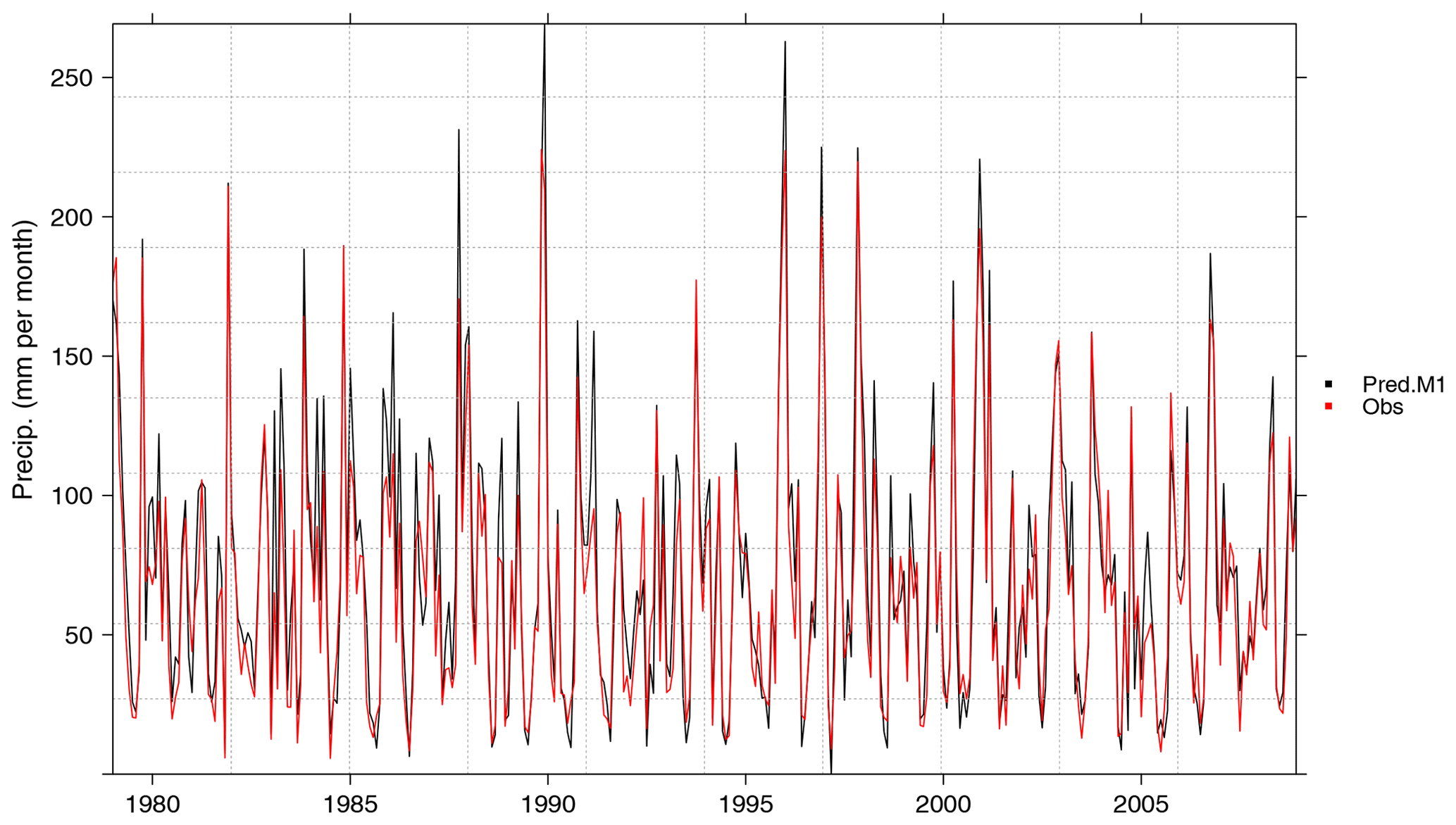
Figure 3Cross-validated predictions of monthly accumulated precipitation by the method M1 (black), plotted against the corresponding observations (red). Both time series have been spatially aggregated considering the 11 stations within the Iberian subdomain.
3.3.3 Configuration of method M2
Unlike M1, in M2 the PCs are independently calculated for each variable, instead of considering one single matrix formed by all joined (combined) variables. To specify this PCA configuration, the spatial predictor parameter list is modified accordingly, by setting which.combine = NULL.
spatial.pars.M2 <- list(which.combine
 = NULL, v.exp = .95)
Note that the rotation argument is here omitted, as it is unused by default. This list of PCA arguments is passed to the spatial.predictor argument. The rest of the code to launch the cross-validation for M2 is identical to M1.
3.3.4 Configuration of method M3
Method M3 uses local predictors only. In this case, the first closest neighbor to the predictand location (n=1) is used considering all the predictor variables (as returned by the helper getVarNames(x)). The local parameters list is next defined:
local.pars.M3 <- list(n = 1, vars
 = getVarNames(x))
In addition, the scaling parameters control the raw predictor standardization. Within the cross-validation setup, standardization is undertaken after data splitting. In this particular case (five folds), the four folds forming the training set are jointly standardized. Then, its mean and variance are used for the standardization of the remaining fold (i.e., the test set). Therefore, the standardization parameters are passed to function downscaleCV as a list of arguments controlling the scaling (scaling.pars object; these parameters are passed internally to the function scaleGrid):
scaling.pars <- list(type = "standardize",
                     spatial.frame =
                       "gridbox")
The next steps are similar to those already shown for M1. For clarity, the precipitation amount M3 model is next shown (the binary logistic model of occurrence would use a similar configuration, but changing the model family, as previously shown).
M3cv.cont <- downscaleCV(x = x, y = y,
               method = "GLM",
               family = Gamma(link = "log"),
               condition = "GE", threshold
                = 1,
               folds = folds,
               scaleGrid.args = scaling.pars,
               prepareData.args =
                list(global.vars = NULL,
                  local.predictors
                  = local.pars.M3,
                  spatial.predictors
                  = NULL))
3.3.5 Configuration of method M4
Method M4 is similar to M3, but using the four closest predictor grid boxes, instead of just one. Thus, the local predictor parameters are slightly modified, by setting n = 4:
local.pars.M4 <- list(n = 4, vars = vars)
3.3.6 Configuration of method M5
Method M5 uses raw (standardized) spatial predictor fields, instead of PCA-transformed ones. The standardization is performed by centering every grid box with respect to the overall spatial mean in order to preserve the spatial consistency of the standardized field. To account for this particularity, the scaling parameters are modified accordingly, via the argument spatial.frame = "field", which is internally passed to scaleGrid.
scaling.pars.M5 <- list(type =
  "standardize",
                        spatial.frame
                         = "field")
In this case, the method for model training is set to analogs. Other specific arguments for analog method tuning are used, for instance, the number of analogs considered (1 in this case):
M5cv <- downscaleCV(x = x, y = y,
          method = "analogs", n.analogs
           = 1,
          folds = folds,
          scaleGrid.args = scaling.pars.M5,
          prepareData.args =
           list(global.vars = vars,
             local.predictors = NULL,
             spatial.predictors = NULL))
3.3.7 Configuration of method M6
The parameters used for predictor configuration in method M6 (combined PCs explaining 95 % of total variance) are similar to method M1. Thus, the previously defined parameter list spatial.pars.M1 is reused here:
M6cv <- downscaleCV(x = x, y = y,
          method = "analogs", n.analogs
           = 1,
          folds = folds,
          prepareData.args =
           list(global.vars = NULL,
             local.predictors = NULL,
             spatial.predictors =
               spatial.pars.M1,
             combined.only = TRUE))
3.3.8 Configuration of method M7
Similarly, method M7 uses identical spatial parameters as previously used for method M2 (parameter list spatial.pars.M2), the rest of the code being similar to M6 but setting combined.only = FALSE, as independent PCs are used instead of the combined one.
3.3.9 Validation
Once the cross-validated predictions for the methods M1 to M7 are generated, their evaluation is undertaken following the systematic approach of the VALUE framework. For brevity, in this example the code of only two example indices is shown: relative wet-day frequency (R01) and simple day intensity index (SDII). The evaluation considering a more complete set of nine validation indices is included in the supplementary notebook to this paper (see the “Code and data availability” section), following the subset of measures used in the VALUE synthesis paper by Gutiérrez et al. (2019). Alternatively, a complete list of indices and measures and their definitions is available in a dedicated section in the VALUE Validation Portal (http://www.value-cost.eu/validationportal/app/#!indices, last access: 29 March 2020). It is also possible to have a quick overview of the available indices and measures within the R session by using the helper functions VALUE::show.indices() and VALUE::show.measures().
To apply them, the package climate4R.value, already introduced in Sect. 2.3, is used. The function valueMeasure is the workhorse for computing all the measures defined by the VALUE Framework. For example, to compute the ratio of the frequency of wet days (VALUE code R01) for a given cross-validated method (M6 in this example), the parameters measure.code="ratio" and index.code="R01" are given:
R01.ratio <- valueMeasure(y, x = M6cv,
                 measure.code = "ratio",
                 index.code = "R01")$Measure
A spatial plot helps to identify at a glance at which locations the frequency of wet days is under- or overestimated (red and blue, respectively) by method M6 (Fig. 4):
## Generates Fig. 4:
spatialPlot(R01.ratio, backdrop.theme
 = "countries")

Figure 4Cross-validation results obtained by method M6, considering the ratio (predicted∕observed) of the frequency of wet days (VALUE index code R01, Table 1).
Following this example and using the nine indices used in the synthesis of the VALUE experiment results (Maraun et al., 2019b) and considering the battery of all methods, M1 to M7, a summary of the validation is presented in Fig. 5. The figure has been generated with the function violinPlot from package visualizeR, as illustrated step by step in the notebook accompanying this paper (see the “Code and data availability” section). Violins are in essence a combination of a box plot and a kernel density plot. Box plots are a standard tool for inspecting the distribution of data most users are familiar with, but they lack basic information when data are not normally distributed. Density plots are more useful when it comes to comparing how different datasets are distributed. For this reason, violin plots incorporate the information of kernel density plots in a box-plot-like representation and are particularly useful to detect bimodalities or departures from the normal distribution of the data, intuitively depicted by the shape of the violins. The violins are internally produced by the package lattice (Sarkar, 2008) via the panel function panel.violin to which the interested reader is referred for further details on violin plot design and options. All the optional graphical parameters of the original panel.violin function can be conveniently passed to the wrapper violinPlot of package visualizeR. In the following, the violin plots shown display how the different validation measures are distributed across locations.
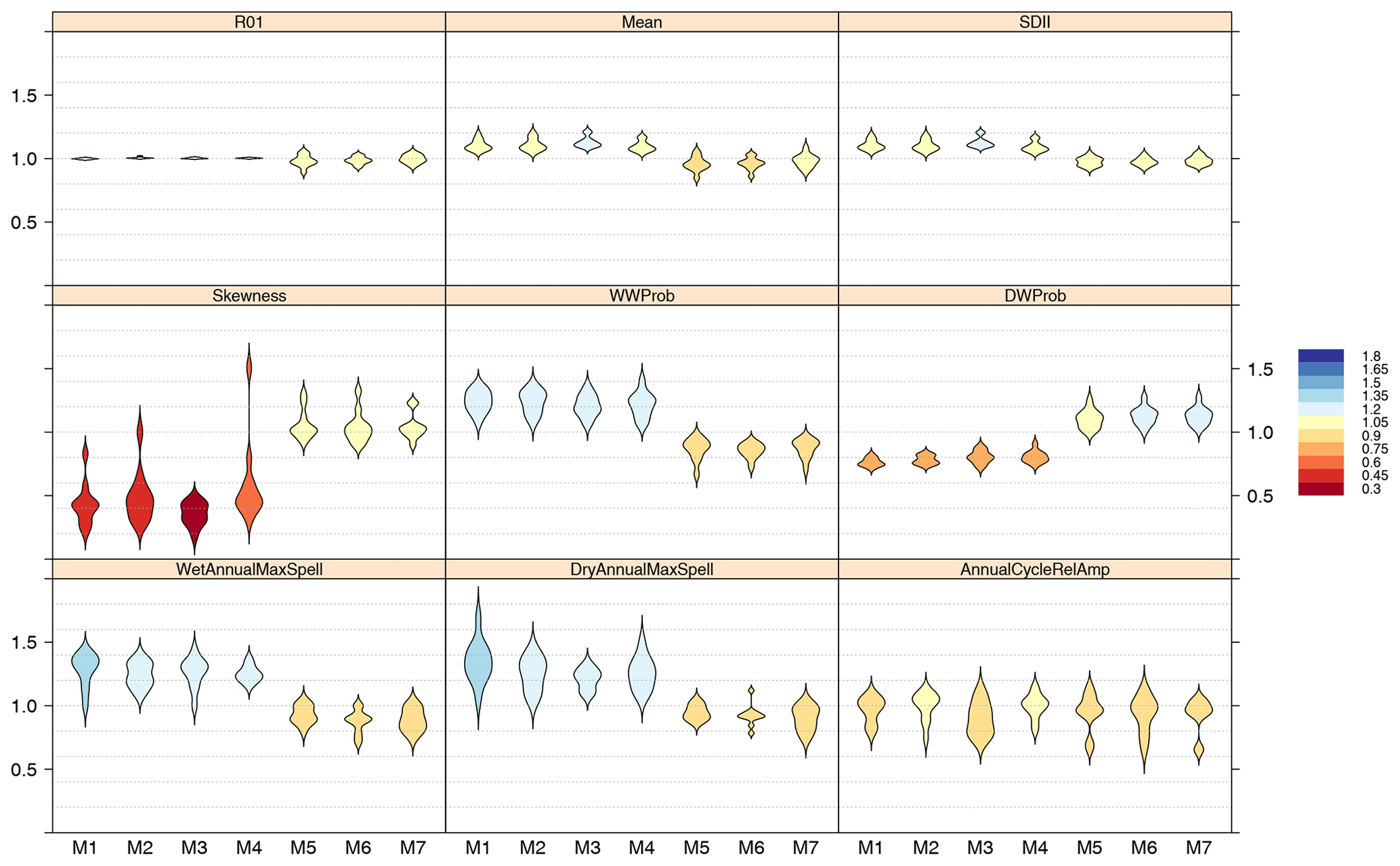
Figure 5Cross-validation results obtained by the seven methods tested (M1 to M7, Table 2) according to the core set of validation indices defined in the VALUE intercomparison experiment, considering the subset of the Iberian Peninsula stations (n=11). The color bar indicates the mean ratio (predicted∕observed) measure calculated for each validation index (Table 1).
The methods M1* and M6* (see Table 2) contributed to the VALUE intercomparison experiment (see methods GLM-DET and ANALOGS in Gutiérrez et al., 2019, Table 3) over the whole European domain, exhibiting a good overall performance. In this section we investigate the potential added value of including local information to these methods. To this aim, the VALUE M1* and M6* configurations are modified by including local information from neighboring predictor grid boxes (these configurations are labeled M1-L and M6-L, respectively; Table 2). The M1-L and M6-L models are trained considering the whole pan-European domain, instead of each subregion independently, taking advantage of the incorporation of the local information at each predictand location and thus disregarding the intermediate step of subsetting across subregions prior to model calibration. The experiment seeks to explore if the more straightforward local predictor approach (M1-L and M6-L) is competitive against the corresponding M1 and M6 VALUE methods when trained with one single, pan-European domain, instead of using the VALUE subregional division, which poses a clear advantage from the user point of view as it does not require testing different spatial domains and the definition of subregions in large downscaling experiments.
Throughout this section, the pan-European experiment is launched and its results presented. Note that now the predictor multigrid corresponds to the whole European domain and the predictand contains the full set of VALUE stations (Fig. 2). The procedure for loading these data is identical to the one already presented in Sect. 3.2.1 and 3.2.2 but considering the European domain. This is achieved by introducing the bounding box defined by the arguments lonLim = c(-10,32) and latLim = c(36,72) in the call to the loadGridData function. These arguments can be omitted in the case of the station data load, since all the available stations are requested in this case. The full code used in this step is detailed in the notebook accompanying this paper (see the “Code and data availability” section).
4.1 Method intercomparison experiment
The configuration of predictors is indicated through the parameter lists, as shown throughout Sects. 3.3.2 to 3.3.8. In the case of method M1-L, local predictors considering the first nearest grid box are included in the M1 configuration (Table 2):
M1.L <- list(local.predictors =
          list(n = 1, vars = vars),
             spatial.predictors =
               list(v.exp = .95,
                 which.combine = vars))
Unlike M6, the M6-L configuration considers local predictors only instead of PCs. In this case, the local domain window is wider than for M1-L, including the 25 closest grid boxes instead of just one:
M6.L <- list(local.predictors = list(n = 25,
  vars = vars))
Next, the cross-validation is launched using downscaleCV. M1-L corresponds to the GLM method (thus requiring the two models for occurrence and amount), while M6-L is an analog method. After this, the validation is undertaken using valueMeasure. PP methods in general build on a synchronous daily link established between predictor(s) and predictand in the training phase (Sect. 2). The strength of this link indicates the local variability explained by the method as a function of the large-scale predictors. In order to provide a quick diagnostic of this strength for the different methods and at the same time to illustrate a diversity of validation methods, in this case correlation, root mean square error, and variance ratio are chosen as validation measures in the validation (Table 1). The validation results are displayed in Fig. 6. For brevity, the code performing the validation of the pan-European experiment is not repeated here (this is similar to what it has been already shown in Sect. 3.3.2 to 3.3.8). The validation results indicate that the local predictor counterparts of the original VALUE methods M1 and M6 are competitive (they reach very similar or slightly better performance in all cases). Hence, the M1-L and M6-L method configurations will be used in Sect. 4.2 to produce the future precipitation projections for Europe, provided their more straightforward application as they do not need to be applied independently for each subregion. While the GLM method improves the correlation between predicted and observed series, the analog approach does a better job at preserving the observed variability.
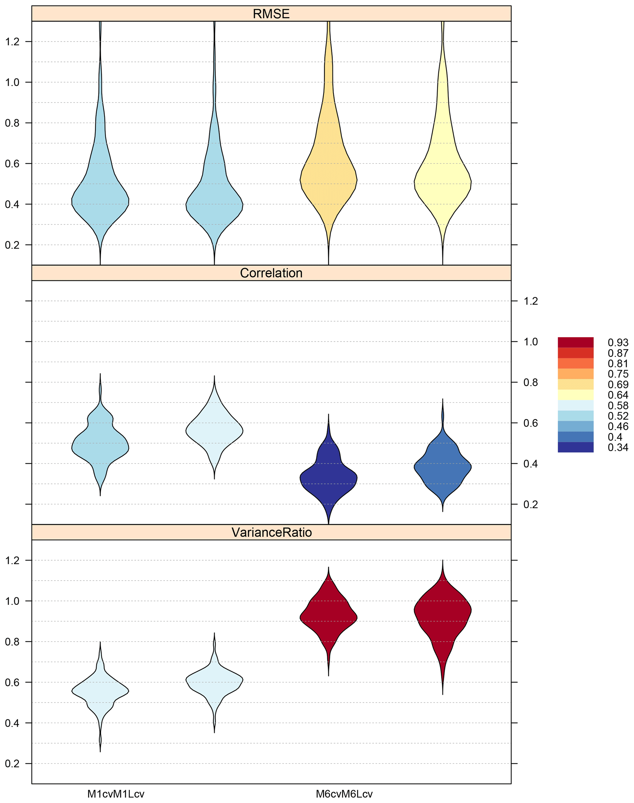
Figure 6Cross-validation results obtained by the four methods tested (M1, M1-L, M6, and M6-L; Table 2) in the pan-European experiment (n=86 stations), according to three selected validation measures (Spearman correlation, RMSE, and variance ratio; see Table 1). The color bar indicates the mean value of each measure. A factor of 0.1 has been applied to the RMSE in order to attain the same order of magnitude in the y axis for all the validation measures.
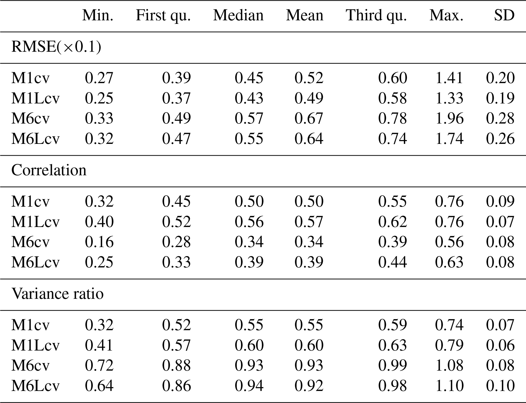
Table 3Validation results of the four methods tested in the pan-European experiment. The values presented (from left to right: minimum, first quartile, median, third quartile, maximum, and standard deviation) correspond to the violin plots displayed in Fig. 6 (n=86 stations). Note that, for consistency with Fig. 6, the RMSE results are multiplied by a factor of 0.1 in order to attain a similar order of magnitude for the three validation measures considered. This is also indicated in the caption of Fig. 6.
4.2 Future downscaled projections
In this section, the calibrated SDS models are used to downscale GCM future climate projections from the CMIP5 EC-EARTH model (Sect. 3.1.3). Before generating the model predictions (Sect. 4.2.2), the perfect-prognosis assumption regarding the good representation by the GCM of the reanalysis predictors is assessed in Sect. 4.2.1.
4.2.1 Assessing the GCM representation of the predictors
As indicated in Sect. 2.1, PP model predictions are built under the assumption that the GCM is able to adequately reproduce the predictors taken from the reanalysis. Here, this question is addressed through the evaluation of the distributional similarity between the predictor variables, as represented by the EC-EARTH model in the historical simulation, and the ERA-Interim reanalysis. To this aim, the two-sample Kolmogorov–Smirnov test is used, included in the set of validation measures of the VALUE framework and thus implemented in the VALUE package. The KS test is a non-parametric statistical hypothesis test for checking the null hypothesis (H0) that two candidate datasets come from the same underlying theoretical distribution. The statistic is bounded between 0 and 1, indicating that the lower values have a greater distributional similarity. The KS test is first applied to the EC-EARTH and ERA-Interim reanalysis time series on a grid box basis, considering the original continuous daily time series for their common period, 1979–2005. In order to isolate distributional dissimilarities due to errors in the first- and second-order moments, we also consider anomalies and standardized anomalies (the latter being used as actual predictors in the SDS models). The anomalies are calculated by removing the overall grid box mean to each daily value, and in the case of the standardized anomalies, we additionally divide by the seasonal standard deviation. Due to the strong serial correlation present in the daily time series, the test is prone to inflation of type-1 error, that is, rejecting the null hypothesis of equal distributions when it is actually true. To this aim, an effective sample size correction has been applied to the data series to calculate the p values (Wilks, 2006). The methodology follows the procedure described in Brands et al. (2012, 2013), implemented by the VALUE measure “ts.ks.pval” (Table 1).
The distributions of GCM and reanalysis (Fig. 7) differ significantly when considering the raw time series, thus violating the assumptions of the PP hypothesis. Centering the data (i.e, zero mean time series) greatly alleviates this problem for most variables, excepting specific humidity at 500 mb (“hus@500”) and near-surface temperature (tas; not shown here, but displayed in the paper notebook). Finally, data standardization improves the distributional similarity, attaining an optimal representation of all the GCM predictors but hus@500 over a few grid points in the Mediterranean.
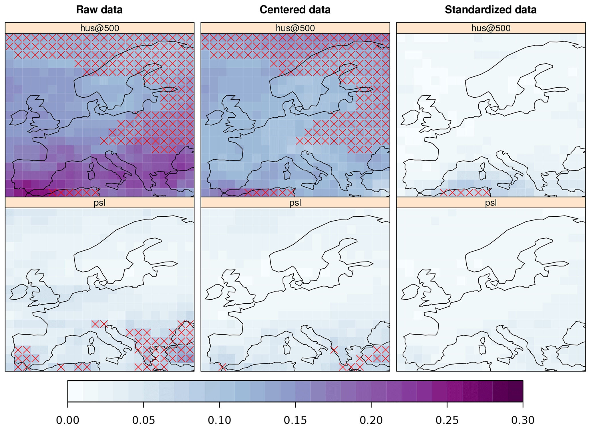
Figure 7KS score maps, depicting the results of the two-sample KS test applied to the time series from the EC-EARTH GCM and ERA-Interim, considering the complete time series for the period 1979–2005. The results are displayed for two of the predictor variables (by rows), namely specific humidity at 500 mb surface pressure height (“hus@500”, badly represented by the GCM) and mean sea-level pressure (“psl”, well represented by the GCM). The KS test results are displayed by columns, using, from left to right, the raw, the zero-mean (centered), and the zero-mean and unit variance (standardized) time series from both the reanalysis and the GCM. The grid boxes showing low p values (p<0.05) have been marked with a red cross, indicating significant differences in the distribution of both GCM and reanalysis time series.
The distributional similarity analysis is straightforward using the functions available in climate4R, already shown in the previous examples. For brevity, the code generating Fig. 7 is omitted here, and included with extended details and for all the predictor variables in the notebook accompanying this paper (see the “Code and data availability” section).
-
Data centering or standardization is performed directly using the function
scaleGridand using the appropriate argument valuestype="center"or"standardize", respectively. -
The KS test is directly launched using the function
valueMeasurefrom the packageclimate4R.VALUEand including the argument valuemeasure.code="ts.ks"and"ts.ks.pval"for KS score and its (corrected) p value, respectively. -
The KS score maps and the stippling based on their p values are produced with the function
spatialPlotfrom packagevisualizeR.
In conclusion, although not all predictors are equally well represented by the GCM, data standardization is able to solve the problem of distributional dissimilarities, even in the case of the worst represented variable, that is, specific humidity at 500 mb level.
4.2.2 Future SDS model predictions
The final configuration of predictors for M1-L (stored in the M1.L list) and M6-L methods (M6.L) is directly passed to the function prepareData, whose output contains all the information required to undertake model training via the downscaleTrain function. In the following, the code for the analog method is presented. Note that for GLMs the code is similar but taking into account occurrence and amount in separated models, as previously shown.
Unlike downscaleCV, which handles predictor standardization on a fold-by-fold basis (see Sect. 3.3.1 in the configuration of method M3), predictor standardization needs to be undertaken prior to passing the predictors to the function prepareData.
# Standardization
x_scale <- scaleGrid(x, type =
 "standardize")
# Predictor config (M6-L method)
M6L <- prepareData(x_scale, y,
  local.predictors = M6.L)
# SDS model training
model.M6L <- downscaleTrain(M6L, method
    = "analogs",
                          n.analogs = 1)
After SDS model calibration downscalePredict is the workhorse for downscaling. First of all, the GCM datasets required are obtained. As previously done with ERA-Interim, the EC-EARTH simulations are obtained from the climate4R UDG, considering the same set of variables already used for training the models (Sect. 3.1.2). Again, the individual predictor fields are recursively loaded and stored in a climate4R multigrid.
historical.dataset <-
 "CMIP5_EC-EARTH_r12i1p1_historical"
grid.list <- lapply(variables, function(x) {
                loadGridData(dataset =
                 historical.dataset,
                    var = x,
                    lonLim = c(-10,32),
                    latLim = c(36,72),
                    years = 1979:2005)
    }
)
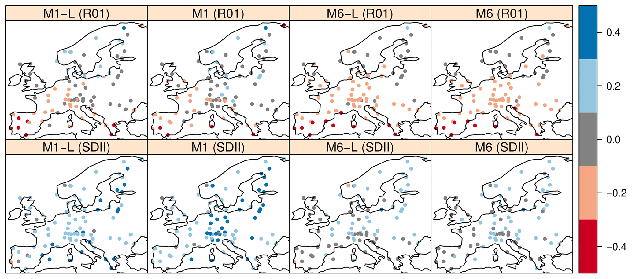
Figure 8Relative delta change signals of the R01 and SDII precipitation indices (see Table 1) for the future period 2071–2100 (with regard to the baseline 1979–2005), obtained by the downscaled projections of the CMIP5 GCM EC-EARTH-r12i1p1, considering the RCP8.5 experiment. The SDS methods used are M1-L, M1, M6, and M6-L (see Table 2).
As done with the predictor set, the prediction dataset is also stored in as a multigrid object:
xh <- makeMultiGrid(grid.list)
An additional step entails regridding the GCM data onto the predictor grid prior to downscaling in order to attain spatial consistency between the predictors and the new prediction data. This is done using the interpGrid function from transformeR:
xh <- interpGrid(xh, new.coordinates =
 getGrid(x))
Identical steps are followed in order to load the future data from RCP8.5. Note that in this case, it suffices to replace the URL pointing to the historical simulation dataset by the one of the future scenario chosen, in this case dataset = "CMIP5_EC-EARTH_r12i1p1_rcp85". The multigrid object storing the future GCM data for prediction will be named xf.
Prior to model prediction, data harmonization is required. This step consists of rescaling the GCM data to conform to the mean and variance of the predictor set that was used to calibrate the model. Note that this step is achieved through two consecutive calls to scaleGrid:
xh <- scaleGrid(xh, base = xh, ref = x,
        type = "center",
        spatial.frame = "gridbox",
        time.frame = "monthly")
xh <- scaleGrid(xh, base = x, type =
  "standardize")
Again, an identical operation is undertaken with the future dataset, by just replacing xh by xf in the previous code chunk. Then, the function prepareNewData will undertake all the necessary data collocation operations, including spatial and temporal checks for consistency, leaving the data structure ready for prediction via downscalePredict. This step is performed equally for the historical and the future scenarios:
h_analog <- prepareNewData(newdata = xh,
 data.struc = M6L)
f_analog <- prepareNewData(newdata = xf,
 data.struc = M6L)
Finally, the predictions for both the historical and the future scenarios are done with downscalePredict. The function receives two arguments: (i) newdata, where the preprocessed GCM predictors after prepareNewData are stored, and (ii) model, which contains the model previously calibrated with downscaleTrain:
hist_ocu_glm <- downscalePredict(newdata
                     = h_analog,
                      model = model.M6L)
Once the downscaled future projections for historical and RCP 8.5 scenarios are produced using the methods M1-L (GLMs) and M6-L (analogs), their respective predicted climate change signals (or “deltas”) are displayed in Fig. 8 (the code to generate the figure is illustrated in the notebook accompanying this paper; see the “Code and data availability” section). We also depict the downscaled climate change signals for the M1 and M6 configurations in order to evaluate whether the local-window approach alters the climate change signals. As illustrated in Fig. 8, the projected relative changes in the climate signal of the R01 (first row) and SDII (second row) indices show minor differences among the configurations presented herein (i.e., M1-L and M6-L) and the VALUE methods (i.e., M1 and M6), showing that the uncertainty due to the SDS method in the climate change signal (M1, GLMs vs. M6, analogs) is larger than that between global predictors or local window (M1/M6 vs. M1-L/M6-L, respectively), in agreement with San-Martín et al. (2016). This result further supports the idea of replacing the VALUE subdomain approach by the adaptive window centered on each predictand location, allowing for a much more straightforward performance of large PP experiments encompassing large areas without the need for testing different subdomain configurations.
The results obtained in the pan-European method intercomparison experiment (Sect. 4.1), indicate that the example SDS methods contributing to the VALUE Experiment (GLMs and analogs, first reproduced in Sect. 3.3.1) can be improved through the incorporation of local predictors, a novel feature brought by downscaleR that can help to avoid the burden of spatial domain screening. It has been shown that this method does not significantly alter the SDS model results, neither in current climate validation nor with regard to the projected anomalies. These results are of relevance for the development of the forthcoming EURO-CORDEX SDS statistical downscaling scenarios, in which the VALUE activities have merged and will follow on, greatly facilitating the development of downscaling experiments over large areas, like the continental scale considered in this study. As in any other experiment, caution must be taken in order to ensure that the assumptions for perfect-prognosis applications are fulfilled, as shown here.
The experiments carried out throughout Sects. 3.3 and 4 have served to the purpose of showcasing the most prominent features of the R package downscaleR and its integration in the climate4R framework, demonstrating its use in end-to-end applications. In this regard, downscaleR is a new tool implementing state-of-the-art SDS techniques providing an extremely flexible interface to accomplish complex downscaling experiments. Critical aspects to be considered in any downscaling exercise, including domain definition, predictor configuration, perfect-prognosis hypothesis testing, model validation, and intercomparison, can be achieved through the use of a few intuitive commands. Users of downscaleR can also benefit from its direct integration within the comprehensive, well-consolidated VALUE framework for model evaluation. Furthermore, its full integration with climate4R brings to climate scientists and practitioners a unique comprehensive R-based framework for SDS model development, including a cloud-computing facility, user-friendly data access to a large climate database, and efficient solutions for data manipulation, visualization and analysis within one single computing environment.
A1 Method
The computing performance of the different downscaling experiments is analyzed in this Appendix through the use of one indicator, the computing time, which measures the (user) time required to accomplish a certain task. Therefore, all timings presented in the following plots correspond to user (wall) times. The values shown are mean values after considering n=10 experiment replicates in all cases. However, spread measures are not displayed given that their values are negligible, attaining all realizations very similar timings.
All timings presented have been measured using the R package microbenchmark (Mersmann, 2019), on a dedicated Ubuntu 16.04 LTS (64 bits), with 15.6 GiB memory and a multi-core CPU composed of eight processing units Intel® Core™ i7-6700 of 3.40 GHz. Further details on the R configuration are provided in the “Session information” section of the notebook accompanying this paper.
A2 Results
The computing times for the Iberia and pan-European downscaling experiments are depicted in Figs. A1 and A2, respectively. A more detailed description of the process naming is indicated in Table A1. The different downscaling configurations are named according to Table 2 and match the nomenclature used in the notebook accompanying this paper. As it can be seen, all the method families perform similarly, the analogs approach in general being significantly slower than GLMs, highlighting the computationally demanding task of analog search (methods M5–M7), which is significantly reduced when the dimensionality of the predictor set is reduced using PCs (M6 and M7). On the other hand, the use of local neighbors instead of PCs does not make a significant difference in computing times, as it can be seen from the intercomparison of GLM methods (M1 to M4, Fig. A1). As expected, downscaling the pan-European domain (i.e., configurations M1L and M6L) leads to higher computational times in comparison with the Iberian downscaling experiment (see Fig. A2), especially in the analog case, in which the analog search is computationally demanding due to the larger size of the Europe-wide predictor set. The comparison between training and testing times shows that the most time-consuming sub-task is the preparation of the predictor and SDS model training, in this order (Fig. A3), while prediction is much faster in general for all the methods.
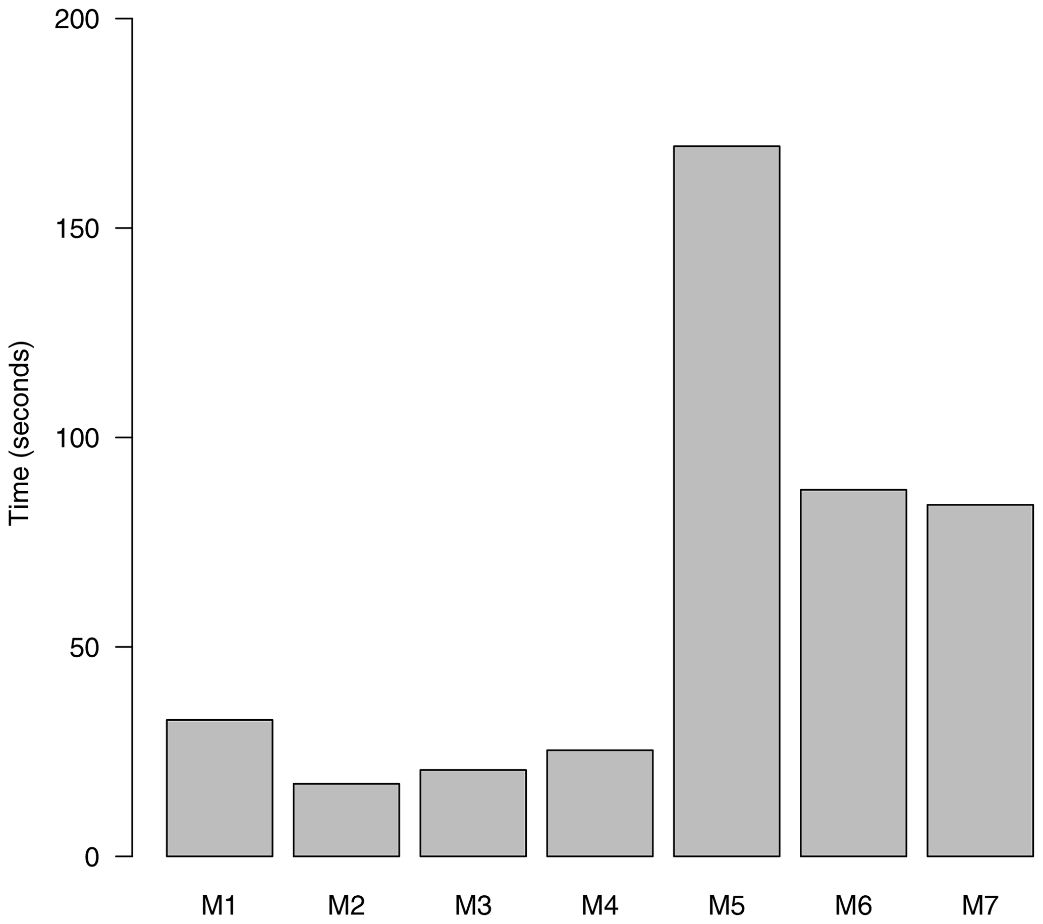
Figure A1Cross-validation times required for the downscaling models developed in the Iberian experiment. The computational times of the generalized linear models configurations (see Table A1) includes both the downscaling of the occurrence and amount of precipitation, whereas for the analogs both aspects are downscaled simultaneously. More information about the configurations can be found in Tables A1 and 2 or in the notebook accompanying this paper.
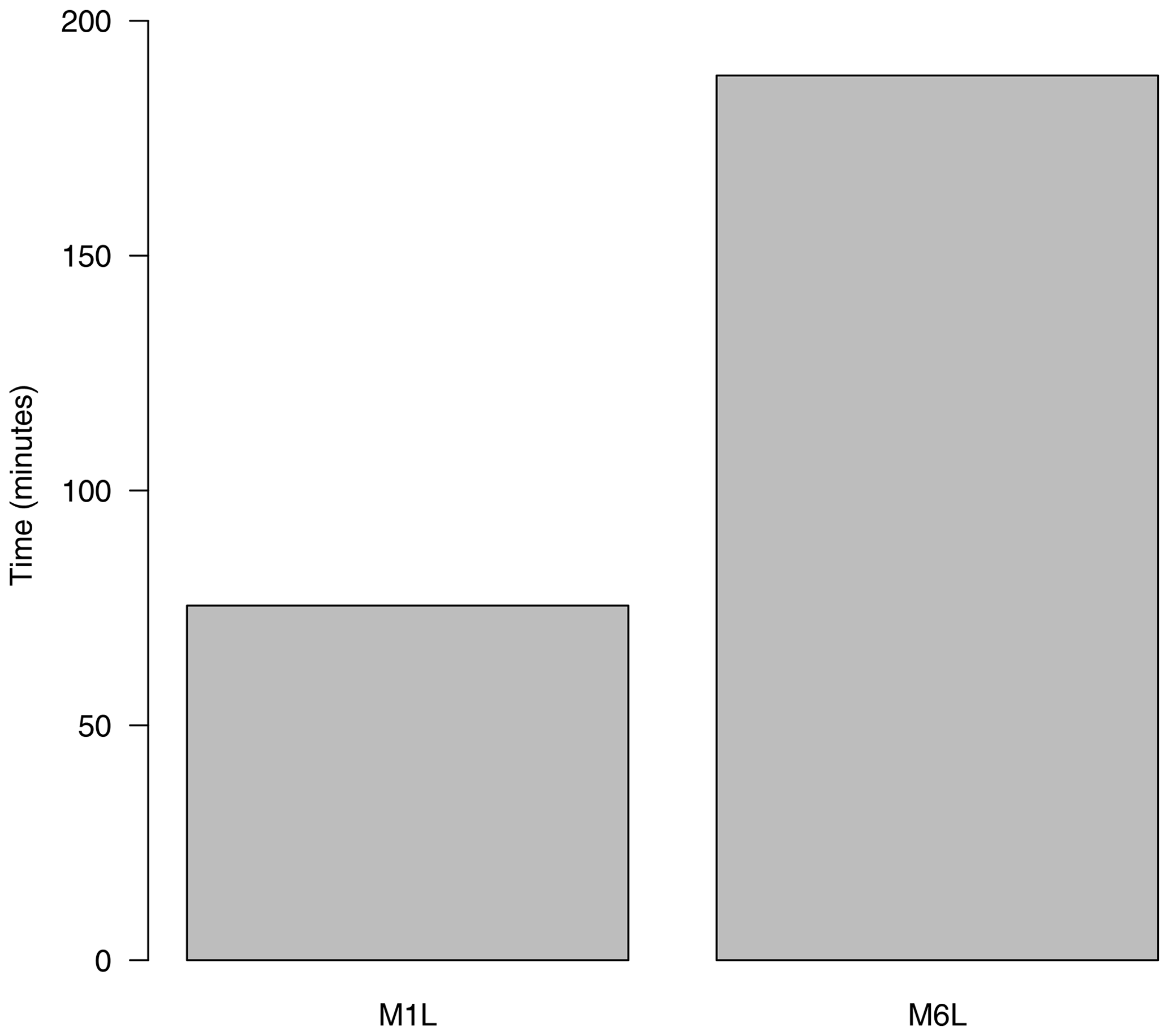
Figure A2Cross-validation times required for the downscaling models developed in the pan-European experiment. The computational times of the generalized linear models configurations (see Table A1) includes both the downscaling of the occurrence and amount of precipitation, whereas for the analogs both aspects are downscaled simultaneously. More information about the configurations can be found in Tables A1 and 2 or in the notebook accompanying this paper.

Figure A3Computing times of a particular method (M1-L for precip. occurrence, Table A1) considering the European domain experiment (n=86 stations, 1979–2008). The bulk of computing time is for predictor preparation and model fitting, while the preparation of the new data and the predictions are relatively much faster.
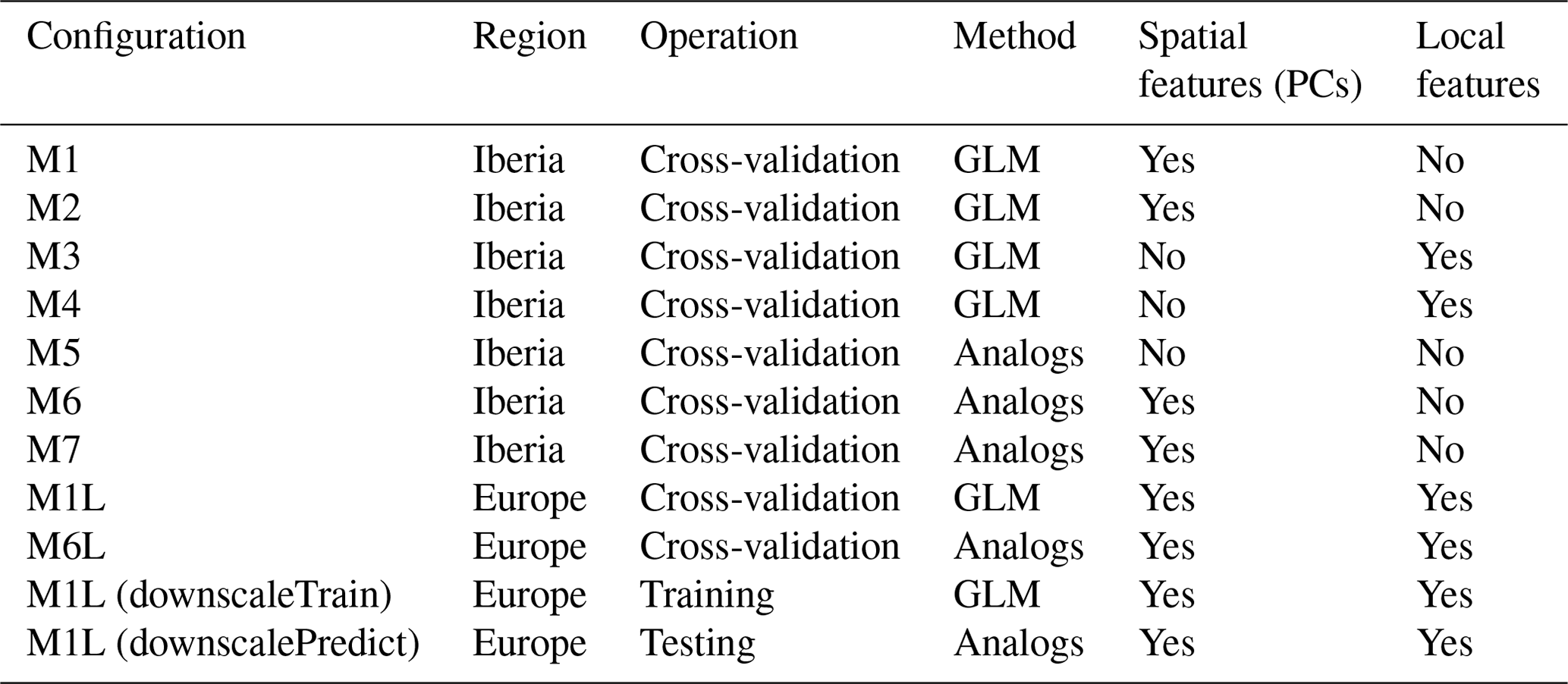
In order to promote transparency and research reproducibility, all the steps followed to generate the analyses shown in this paper (with extended details and additional information) are available in the notebook accompanying this paper (repo version 0.1.4, https://doi.org/10.5281/zenodo.3567736, Bedia et al., 2019b):
-
source file (R markdown): https://github.com/SantanderMetGroup/notebooks/blob/v0.1.4/2019_downscaleR_GMD.Rmd (last access: 29 March 2020)
-
html file: https://github.com/SantanderMetGroup/notebooks/blob/v0.1.4/2019_downscaleR_GMD.html (last access: 29 March 2020)
-
pdf file: https://github.com/SantanderMetGroup/notebooks/blob/v0.1.4/2019_downscaleR_GMD.pdf (last access: 29 March 2020).
The R software and all the packages required to reproduce the results are freely available as indicated in the paper notebook, where more specific details for installation and required versions are given.
-
Name of the software:
downscaleR(paper version: 3.1.0, https://doi.org/10.5281/zenodo.3277316, Bedia et al., 2019b) -
Developers: authors of this paper
-
Website: https://github.com/SantanderMetGroup/downscaleR (last access: 29 March 2020)
-
Hardware requirements: general-purpose computer
-
Programming languages: R
-
Software requirements: R version 3.1.0 or later.
All the authors have contributed to the downscaleR package development. JB, JBM, and JMG wrote an initial version of the paper and designed the illustrative experiments. JB and JBM prepared the notebook accompanying this paper and the analyses shown in the Appendix.
The authors declare that they have no conflict of interest.
We thank the European Union Cooperation in Science and Technology (EU COST) Action ES1102 VALUE (http://www.value-cost.eu) for making publicly available the data used in this article and the tools implementing the comprehensive set of validation measures and indices. We also thank the THREDDS Data Server (TDS) software developed by UCAR/Unidata (https://doi.org/10.5065/D6N014KG, Unidata, 2006) and all R developers and their supporting community for providing free software facilitating open science. We acknowledge the World Climate Research Program's Working Group on Coupled Modelling, which is responsible for CMIP, and we thank the EC-EARTH Consortium for producing and making available their model output used in this paper. For CMIP the U.S. Department of Energy's Program for Climate Model Diagnosis and Intercomparison provides coordinating support and led the development of software infrastructure in partnership with the Global Organization for Earth System Science Portals. We are very grateful to the two anonymous referees participating in the interactive discussion for their insightful comments, helping us to considerably improve the original paper.
The authors acknowledge partial funding from the MULTI-SDM project (MINECO/FEDER, CGL2015-66583-R) and from the project INDECIS, part of the European Research Area for Climate Services Consortium (ERA4CS) with co-funding by the European Union (grant no. 690462).
This paper was edited by Olaf Morgenstern and reviewed by two anonymous referees.
Abaurrea, J. and Asín, J.: Forecasting local daily precipitation patterns in a climate change scenario, Clim. Res., 28, 183–197, https://doi.org/10.3354/cr028183, 2005. a
Baño-Medina, J., Manzanas, R., and Gutiérrez, J. M.: Configuration and Intercomparison of Deep Learning Neural Models for Statistical Downscaling, Geosci. Model Dev. Discuss., https://doi.org/10.5194/gmd-2019-278, in review, 2019. a
Barsugli, J. J., Guentchev, G., Horton, R. M., Wood, A., Mearns, L. O., Liang, X.-Z., Winkler, J. A., Dixon, K., Hayhoe, K., Rood, R. B., Goddard, L., Ray, A., Buja, L., and Ammann, C.: The Practitioner's Dilemma: How to Assess the Credibility of Downscaled Climate Projections, Eos T. Am. Geophys. Un., 94, 424–425, https://doi.org/10.1002/2013EO460005, 2013. a
Bedia, J., Herrera, S., San-Martín, D., Koutsias, N., and Gutiérrez, J. M.: Robust projections of Fire Weather Index in the Mediterranean using statistical downscaling, Climatic Change, 120, 229–247, https://doi.org/10.1007/s10584-013-0787-3, 2013. a
Bedia, J., Golding, N., Casanueva, A., Iturbide, M., Buontempo, C., and Gutiérrez, J.: Seasonal predictions of Fire Weather Index: Paving the way for their operational applicability in Mediterranean Europe, Climate Services, 9, 101–110, https://doi.org/10.1016/j.cliser.2017.04.001, 2018. a
Bedia, J., San-Martín, D., Iturbide, M., Herrera, S., Manzanas, R., and Gutiérrez, J. M.: The METACLIP semantic provenance framework for climate products, Environ. Modell. Softw., 119, 445–457, https://doi.org/10.1016/j.envsoft.2019.07.005, 2019a. a
Bedia, J., Baño-Medina, J., Casanueva, A., Cofiño, A. S., Gutiérrez, J. M., Herrera, S., Iturbide, M., Legasa, M.N., Manzanas, R., and San-Martín, D.: Paper notebook repository of the Santander Meteorology Group, https://doi.org/10.5281/zenodo.3277316, 2019b. a, b
Benestad, R.: Novel methods for inferring future changes in extreme rainfall over Northern Europe, Clim. Res., 34, 195–210, https://doi.org/10.3354/cr00693, 2007. a
Benestad, R. E.: A comparison between two empirical downscaling strategies, International J. Climatol., 21, 1645–1668, https://doi.org/10.1002/joc.703, 2001. a, b
Benestad, R. E.: Downscaling precipitation extremes: Correction of analog models through PDF predictions, Theor. Appl. Climatol., 100, 1–21, https://doi.org/10.1007/s00704-009-0158-1, 2010. a
Benestad, R. E., Mezghani, A., and Parding, K. M.: “esd” – The Empirical-Statistical Downscaling tool & its visualisation capabilities., Tech. rep., Norwegian Meteorological Institute, available at: https://figshare.com/articles/_esd_The_Empirical_Statistical_Downscaling_tool_amp_its_visualisation_capabilities_/1454425 (last access: 30 March 2020), 2015. a
Brands, S., Gutiérrez, J., Herrera, S., and Cofiño, A.: On the Use of Reanalysis Data for Downscaling, J. Climate, 25, 2517–2526, https://doi.org/10.1175/JCLI-D-11-00251.1, 2012. a, b
Brands, S., Gutiérrez, J. M., Herrera, S., and Cofiño, A. S.: On the use of reanalysis data for downscaling, J. Climate, 25, 2517–2526, https://doi.org/10.1175/JCLI-D-11-00251.1, 2012. a
Brands, S., Herrera, S., Fernández, J., and Gutiérrez, J. M.: How well do CMIP5 Earth System Models simulate present climate conditions in Europe and Africa?: A performance comparison for the downscaling community, Clim. Dynam., 41, 803–817, https://doi.org/10.1007/s00382-013-1742-8, 2013. a
Brandsma, T. and Buishand, T. A.: Statistical linkage of daily precipitation in Switzerland to atmospheric circulation and temperature, J. Hydrol., 198, 98–123, https://doi.org/10.1016/S0022-1694(96)03326-4, 1997. a
Bürger, G. and Chen, Y.: Regression-based downscaling of spatial variability for hydrologic applications, J. Hydrol., 311, 299–317, https://doi.org/10.1016/j.jhydrol.2005.01.025, 2005. a
Chandler, R. E. and Wheater, H. S.: Analysis of rainfall variability using generalized linear models: A case study from the west of Ireland, Water Resour. Res., 38, 10, https://doi.org/10.1029/2001WR000906, 2002. a, b, c
Charles, S. P., Bryson, C. B., Whetton, P. H., and Hughes, J. P.: Validation of downscaling models for changed climate conditions: Case study of southwestern Australia, Clim. Res., 12, 1–14, https://doi.org/10.3354/cr012001, 1999. a
Christensen, J. H., Carter, T. R., Rummukainen, M., and Amanatidis, G.: Evaluating the performance and utility of regional climate models: the PRUDENCE project, Climatic Change, 81, 1–6, https://doi.org/10.1007/s10584-006-9211-6, 2007. a
Christensen, J. H., Boberg, F., Christensen, O. B., and Lucas-Picher, P.: On the need for bias correction of regional climate change projections of temperature and precipitation, Geophys. Res. Lett., 35, L20709, https://doi.org/10.1029/2008GL035694, 2008. a
Cinquini, L., Crichton, D., Mattmann, C., Harney, J., Shipman, G., Wang, F., Ananthakrishnan, R., Miller, N., Denvil, S., Morgan, M., Pobre, Z., Bell, G. M., Doutriaux, C., Drach, R., Williams, D., Kershaw, P., Pascoe, S., Gonzalez, E., Fiore, S., and Schweitzer, R.: The Earth System Grid Federation: An open infrastructure for access to distributed geospatial data, Future Gener. Comp. Sy., 36, 400–417, https://doi.org/10.1016/j.future.2013.07.002, 2014. a
Cofiño, A., Bedia, J., Iturbide, M., Vega, M., Herrera, S., Fernández, J., Frías, M., Manzanas, R., and Gutiérrez, J.: The ECOMS User Data Gateway: Towards seasonal forecast data provision and research reproducibility in the era of Climate Services, Climate Services, 9, 33–43, https://doi.org/10.1016/j.cliser.2017.07.001, 2018. a, b
Dee, D. P., Uppala, S. M., Simmons, A. J., Berrisford, P., Poli, P., Kobayashi, S., Andrae, U., Balmaseda, M. A., Balsamo, G., Bauer, P., Bechtold, P., Beljaars, A. C. M., van de Berg, L., Bidlot, J., Bormann, N., Delsol, C., Dragani, R., Fuentes, M., Geer, A. J., Haimberger, L., Healy, S. B., Hersbach, H., Hölm, E. V., Isaksen, L., Kåallberg, P., Köhler, M., Matricardi, M., McNally, A. P., Monge-Sanz, B. M., Morcrette, J., Park, B., Peubey, C., de Rosnay, P., Tavolato, C., Thépaut, J.-N., and Vitart, F.: The ERA-Interim reanalysis: configuration and performance of the data assimilation system, Q. J. Roy. Meteor. Soc., 137, 553–597, 2011. a
EC-Earth Consortium: EC-EARTH model output prepared for CMIP5 rcp85, served by ESGF, Bulletin of the American Meteorological Society, available at: http://cera-www.dkrz.de/WDCC/CMIP5/Compact.jsp?acronym=IHECr8 (last access: 30 March 2020), 2014. a
Fealy, R. and Sweeney, J.: Statistical downscaling of precipitation for a selection of sites in Ireland employing a generalised linear modelling approach, Int. J. Climatol., 27, 2083–2094, https://doi.org/10.1002/joc.1506, 2007. a
Fowler, H. J., Blenkinsop, S., and Tebaldi, C.: Linking climate change modelling to impacts studies: Recent advances in downscaling techniques for hydrological modelling, Int. J. Climatol., 27, 1547–1578, https://doi.org/10.1002/joc.1556, 2007. a
Frías, M. D., Iturbide, M., Manzanas, R., Bedia, J., Fernández, J., Herrera, S., Cofiño, A. S., and Gutiérrez, J. M.: An R package to visualize and communicate uncertainty in seasonal climate prediction, Environ. Modell. Softw., 99, 101–110, https://doi.org/10.1016/j.envsoft.2017.09.008, 2018. a, b
Giorgi, F., Jones, C., and Asrar, G. R.: Addressing climate information needs at the regional level: the CORDEX framework, Bulletin – World Meteorological Organization, 58, 175–183, 2009. a
Glahn, H. R. and Lowry, D. A.: The use of Model Output Statistics (MOS) in objective weather forecasting, J. Appl. Meteorol, 11, 1203–1211, https://doi.org/10.1175/1520-0450(1972)011<1203:TUOMOS>2.0.CO;2, 1972. a
Gutiérrez, J. M., San Martín, D., Cofiño, A. S., Herrera, S., Manzanas, R., and Frías, M. D.: User Guide of the ENSEMBLES Downscaling Portal (version 2), Tech. Rep. 2.2011, Santander Meteorology Group, CSIC-UC, available at: https://meteo.unican.es/downscaling/doc/UserGuide.pdf (last access: 30 March 2020), 2012. a
Gutiérrez, J. M., San-Martín, D., Brands, S., Manzanas, R., and Herrera, S.: Reassessing Statistical Downscaling Techniques for Their Robust Application under Climate Change Conditions, J. Climate, 26, 171–188, https://doi.org/10.1175/JCLI-D-11-00687.1, 2013. a, b, c, d, e
Gutiérrez, J. M., Maraun, D. abd Widmann, M., Huth, R., Hertig, E., Benestad, R., Roessler, R., Wibig, T., Wilcke, R., Kotlarski, S., San-Martín, D., Herrera, S., Bedia, J., Casanueva, A., Manzanas, R., Iturbide, M., and Vrac, M.: An intercomparison of a large ensemble of statistical downscaling methods over Europe: Results from the VALUE perfect predictor cross-validation experiment, Int. J. Climatol., 39, 3750–3785, https://doi.org/10.1002/joc.5462, 2019. a, b, c, d, e, f, g, h, i, j, k
Hanssen-Bauer, I., Achberger, C., Benestad, R. E., Chen, D., and Forland, E. J.: Statistical downscaling of climate scenarios over Scandinavia, Clim. Res., 29, 255–268, https://doi.org/10.3354/cr029255, 2005. a
Haylock, M. R., Cawley, G. C., Harpham, C., Wilby, R. L., and Goodess, C. M.: Downscaling heavy precipitation over the United Kingdom: A comparison of dynamical and statistical methods and their future scenarios, Int. J. Climatol., 26, 1397–1415, https://doi.org/10.1002/joc.1318, 2006. a
Hertig, E. and Jacobeit, J.: Assessments of Mediterranean precipitation changes for the 21st century using statistical downscaling techniques, Int. J. Climatol., 28, 1025–1045, https://doi.org/10.1002/joc.1597, 2008. a
Hertig, E., Seubert, S., Paxian, A., Vogt, G., Paeth, H., and Jacobeit, J.: Changes of total versus extreme precipitation and dry periods until the end of the twenty-first century: Statistical assessments for the Mediterranean area, Theor. Appl. Climatol., 111, 1–20, https://doi.org/10.1007/s00704-012-0639-5, 2013. a
Hertig, E., Maraun, D., Bartholy, J., Pongracz, R., Vrac, M., Mares, I., Gutiérrez, J. M., Wibig, J., Casanueva, A., and Soares, P. M. M.: Comparison of statistical downscaling methods with respect to extreme events over Europe: Validation results from the perfect predictor experiment of the COST Action VALUE, Int. J. Climatol., 39, 3846–3867, https://doi.org/10.1002/joc.5469, 2019. a
Huth, R.: Statistical downscaling in central Europe: Evaluation of methods and potential predictors, Clim. Res., 13, 91–101, https://doi.org/10.3354/cr013091, 1999. a
Huth, R.: Sensitivity of Local Daily Temperature Change Estimates to the Selection of Downscaling Models and Predictors, J. Climate, 17, 640–652, https://doi.org/10.1175/1520-0442(2004)017<0640:SOLDTC>2.0.CO;2, 2004. a
Iturbide, M., Bedia, J., and Gutiérrez, J. M.: Tackling Uncertainties of Species Distribution Model Projections with Package mopa, The R Journal, 10, 122–139, 2018. a
Iturbide, M., Bedia, J., Herrera, S., Baño Medina, J., Fernández, J., Frías, M. D., Manzanas, R., D., S.-M., Cimadevilla, E., Cofiño, J. M., , and Gutiérrez, J. M.: climate4R: An R-based Framework for Climate Data Access,Post-processing and Bias Correction, Environ. Modell. Softwa., 111, 42–54, https://doi.org/10.1016/j.envsoft.2018.09.009, 2019. a, b, c, d, e
Jacob, D., Petersen, J., Eggert, B., Alias, A., Christensen, O. B., Bouwer, L., Braun, A., Colette, A., Déqué, M., Georgievski, G., Georgopoulou, E., Gobiet, A., Menut, L., Nikulin, G., Haensler, A., Hempelmann, N., Jones, C., Keuler, K., Kovats, S., Kröner, N., Kotlarski, S., Kriegsmann, A., Martin, E., van Meijgaard, E., Moseley, C., Pfeifer, S., Preuschmann, S., Radermacher, C., Radtke, K., Rechid, D., Rounsevell, M., Samuelsson, P., Somot, S., Soussana, J.-F., Teichmann, C., Valentini, R., Vautard, R., Weber, B., and Yiou, P.: EURO-CORDEX: new high-resolution climate change projections for European impact research, Reg. Environ. Change, 14, 563–578, https://doi.org/10.1007/s10113-013-0499-2, 2014. a
Klein, W. H., Lewis, B. M., and Enger, I.: Objective prediction of five-day mean temperatures during winter, J. Meteorol., 16, 672–682, https://doi.org/10.1175/1520-0469(1959)016<0672:OPOFDM>2.0.CO;2, 1959. a
Klein Tank, A. M. G., Wijngaard, J. B., Können, G. P., Böhm, R., Demarée, G., Gocheva, A., Mileta, M., Pashiardis, S., Hejkrlik, L., Kern-Hansen, C., Heino, R., Bessemoulin, P., Müller-Westermeier, G., Tzanakou, M., Szalai, S., Pálsdóttir, T., Fitzgerald, D., Rubin, S., Capaldo, M., Maugeri, M., Leitass, A., Bukantis, A., Aberfeld, R., van Engelen, A. F. V., Forland, E., Mietus, M., Coelho, F., Mares, C., Razuvaev, V., Nieplova, E., Cegnar, T., Antonio López, J., Dahlström, B., Moberg, A., Kirchhofer, W., Ceylan, A., Pachaliuk, O., Alexander, L. V., and Petrovic, P.: Daily dataset of 20th-century surface air temperature and precipitation series for the European Climate Assessment, Int. J. Climatol., 22, 1441–1453, https://doi.org/10.1002/joc.773, 2002. a
Kohavi, R.: A Study of Cross-Validation and Bootstrap for Accuracy Estimation and Model Selection, in: Proceedings of the International Joint Conference on Artificial Intelligence, Morgan Kaufmann, 1137–1143, 1995. a
Lachenbruch, P. A. and Mickey, M. R.: Estimation of Error Rates in Discriminant Analysis, Technometrics, 10, 1–11, https://doi.org/10.2307/1266219, 1968. a
Laprise, R.: Regional climate modelling, J. Comput. Phys., 227, 3641–666, https://doi.org/10.1016/j.jcp.2006.10.024, 2008. a
Lorenz, E. N.: Atmospheric predictability as revealed by naturally occurring analogues, J. Atmos. Sci., 26, 636–646, https://doi.org/10.1175/1520-0469(1969)26<636:APARBN>2.0.CO;2, 1969. a
Manzanas, R., Brands, S., San-Martín, D., Lucero, A., Limbo, C., and Gutiérrez, J. M.: Statistical Downscaling in the Tropics Can Be Sensitive to Reanalysis Choice: A Case Study for Precipitation in the Philippines, J. Climate, 28, 4171–4184, https://doi.org/10.1175/JCLI-D-14-00331.1, 2015. a
Manzanas, R., Lucero, A., Weisheimer, A., and Gutiérrez, J. M.: Can bias correction and statistical downscaling methods improve the skill of seasonal precipitation forecasts?, Clim. Dynam., 50, 1161–1176, https://doi.org/10.1007/s00382-017-3668-z, 2017. a, b
Maraun, D. and Widmann, M.: Structure of Statistical Downscaling Methods, Cambridge University Press, 135–140, https://doi.org/10.1017/9781107588783.011, 2018. a, b, c, d
Maraun, D., Widmann, M., Gutiérrez, J. M., Kotlarski, S., Chandler, R. E., Hertig, E., Wibig, J., Huth, R., and Wilcke, R. A.: VALUE: A framework to validate downscaling approaches for climate change studies, Earth's Future, 3, 1–14, https://doi.org/10.1002/2014EF000259, 2015. a, b, c, d
Maraun, D., Huth, R., Gutiérrez, J. M., Martín, D. S., Dubrovsky, M., Fischer, A., Hertig, E., Soares, P. M. M., Bartholy, J., Pongrácz, R., Widmann, M., Casado, M. J., Ramos, P., and Bedia, J.: The VALUE perfect predictor experiment: evaluation of temporal variability, Int. J. Climatol., 39, 3786–3818, https://doi.org/10.1002/joc.5222, 2019a. a
Maraun, D., Widmann, M., and Gutiérrez, J. M.: Statistical downscaling skill under present climate conditions: A synthesis of the VALUE perfect predictor experiment, Int. J. Climatol., 39, 3692–3703, https://doi.org/10.1002/joc.5877, 2019b. a, b, c
Markatou, M., Tian, H., Biswas, S., and Hripcsak, G.: Analysis of Variance of Cross-Validation Estimators of the Generalization Error, J. Mach. Learn. Res., 6, 1127–1168, https://doi.org/10.7916/D86D5R2X, 2005. a
Marzban, C., Sandgathe, S., and Kalnay, E.: MOS, Perfect-Prog and reanalysis, Mon. Weather Rev., 134, 657–663, https://doi.org/10.1175/MWR3088.1, 2006. a
Matulla, C., Zhang, X., Wang, X., Wang, J., Zorita, E., Wagner, S., and von Storch, H.: Influence of similarity measures on the performance of the analog method for downscaling daily precipitation, Clim. Dynam., 30, 133–144, https://doi.org/10.1007/s00382-007-0277-2, 2008. a
Mersmann, O.: microbenchmark: Accurate Timing Functions, r package version 1.4-7, available at: https://CRAN.R-project.org/package=microbenchmark (last access: 30 March 2020), 2019. a
Moss, R. H., Edmonds, J. A., Hibbard, K. A., Manning, M. R., Rose, S. K., van Vuuren, D. P., Carter, T. R., Emori, S., Kainuma, M., Kram, T., Meehl, G. A., Mitchell, J. F. B., Nakicenovic, N., Riahi, K., Smith, S. J., Stouffer, R. J., Thomson, A. M., Weyant, J. P., and Wilbanks, T. J.: The next generation of scenarios for climate change research and assessment, Nature, 463, 747–756, https://doi.org/10.1038/nature08823, 2010. a
Nelder, J. A. and Wedderburn, R. W. M.: Generalized linear models, J. Roy. Stat. Soc. A, 135, 370–384, https://doi.org/10.2307/2344614, 1972. a
Preisendorfer, R.: Principal component analysis in meteorology and oceanography, Elsevier, 1st Edn., 1988. a
R Core Team: R: A Language and Environment for Statistical Computing, R Foundation for Statistical Computing, Vienna, Austria, available at: https://www.R-project.org/ (last access: 30 March 2020), 2019. a
Rössler, O., Fischer, A. M., Huebener, H., Maraun, D., Benestad, R. E., Christodoulides, P., Soares, P. M. M., Cardoso, R. M., Pagé, C., Kanamaru, H., Kreienkamp, F., and Vlachogiannis, D.: Challenges to link climate change data provision and user needs: Perspective from the COST-action VALUE, Int. J. Climatol., 39, 3704–3716, https://doi.org/10.1002/joc.5060, 2019. a
Rummukainen, M.: Methods for Statistical Downscaling of GCM Simulations, Tech. rep., Swedish Meteorological and Hydrological Institute, available at: https://www.smhi.se/polopoly_fs/1.124322!/RMK_80.pdf (last access: 9 July 2019), 1997. a
San-Martín, D., Manzanas, R., Brands, S., Herrera, S., and Gutiérrez, J. M.: Reassessing Model Uncertainty for Regional Projections of Precipitation with an Ensemble of Statistical Downscaling Methods, J. Climate, 30, 203–223, https://doi.org/10.1175/JCLI-D-16-0366.1, 2016. a, b, c, d
Sarkar, D.: Lattice: Multivariate Data Visualization with R, Springer, New York, available at: http://lmdvr.r-forge.r-project.org (last access: 30 March 2020), 2008. a
Sauter, T. and Venema, V.: Natural three-dimensional predictor domains for statistical precipitation downscaling, J. Climate, 24, 6132–6145, https://doi.org/10.1175/2011JCLI4155.1, 2011. a
Soares, P. M. M., Maraun, D., Brands, S., Jury, M. W., Gutiérrez, J. M., San-Martín, D., Hertig, E., Huth, R., Belušić Vozila, A., Cardoso, R. M., Kotlarski, S., Drobinski, P., and Obermann-Hellhund, A.: Process-based evaluation of the VALUE perfect predictor experiment of statistical downscaling methods, Int. J. Climatol., 39, 3868–3893, https://doi.org/10.1002/joc.5911, 2019. a
Sterl, A.: On the (in)homogeneity of reanalysis products, J. Climate, 17, 3866–3873, 2004. a
Stone, M.: Cross-Validatory Choice and Assessment of Statistical Predictions, J. Roy. Stat. Soc. Ser. B, 6, 11–147, 1974. a
Taylor, K. E., Stouffer, R. J., and Meehl, G. A.: An Overview of CMIP5 and the Experiment Design, B. Am. Meteorol. Soc., 93, 485–498, https://doi.org/10.1175/BAMS-D-11-00094.1, 2011. a
Timbal, B., Dufour, A., and McAvaney, B.: An estimate of future climate change for western France using a statistical downscaling technique, Clim. Dynam., 20, 807–823, https://doi.org/10.1007/s00382-002-0298-9, 2003. a
Turco, M., Quintana-Seguí, P., Llasat, M. C., Herrera, S., and Gutiérrez, J. M.: Testing MOS precipitation downscaling for ENSEMBLES regional climate models over Spain, J. Geophys. Res., 116, D18109, https://doi.org/10.1029/2011JD016166, 2011. a
Unidata: NetCDF-Java library and THREDDS Data Server (TDS), Boulder, CO, https://doi.org/10.5065/D6N014KG, 2006. a, b
van der Linden, P. and Mitchell, J.: ENSEMBLES: Climate Change and its Impacts: Summary of research and results from the ENSEMBLES project – European Environment Agency (EEA), Tech. rep., Met Office Hadley Centre, FitzRoy Road, Exeter EX1 3PB, UK, available at: http://www.eea.europa.eu/data-and-maps/indicators/global-and-european-temperature/ensembles-climate-change-and-its (last access: 30 March 2020), 2009. a
von Storch, H., Zorita, E., and Cubasch, U.: Downscaling of global climate change estimates to regional scales: An application to Iberian rainfall in wintertime, J. Climate, 6, 1161–1171, https://doi.org/10.1175/1520-0442(1993)006<1161:DOGCCE>2.0.CO;2, 1993. a
Widmann, M., Bretherton, C. S., and Salathé, E. P.: Statistical Precipitation Downscaling over the Northwestern United States Using Numerically Simulated Precipitation as a Predictor, J. Climate, 16, 799–816, https://doi.org/10.1175/1520-0442(2003)016<0799:SPDOTN>2.0.CO;2, 2003. a
Widmann, M., Bedia, J., Gutiérrez, J., Bosshard, T., Hertig, E., Maraun, D., Casado, M., Ramos, P., Cardoso, R., Soares, P., Ribalaygua, J., Pagé, C., Fischer, A., Herrera, S., and Huth, R.: Validation of spatial variability in downscaling results from the VALUE perfect predictor experiment, Int. J. Climatol., 39, 3819–3845, https://doi.org/10.1002/joc.6024, 2019. a, b
Wilby, R. L., Charles, S., Zorita, E., Timbal, B., Whetton, P., and Mearns, L.: Guidelines for use of climate scenarios developed from statistical downscaling methods, Tech. rep., IPCC-TGCIA, 2004. a
Wilks, D. S.: Statistical methods in the atmospheric sciences, Amsterdam, Elsevier, 2nd Edn., 2006. a
Zorita, E. and von Storch, H.: The Analog Method as a Simple Statistical Downscaling Technique: Comparison with More Complicated Methods, J. Climate, 12, 2474–2489, https://doi.org/10.1175/1520-0442(1999)012<2474:TAMAAS>2.0.CO;2, 1999. a, b
- Abstract
- Introduction
-
Perfect-prognosis SDS:
downscaleR - Illustrative case study: the VALUE experiment
- Contribution to VALUE: further results
- Conclusions
- Appendix A: Computing times
- Code and data availability
- Author contributions
- Competing interests
- Acknowledgements
- Financial support
- Review statement
- References