the Creative Commons Attribution 4.0 License.
the Creative Commons Attribution 4.0 License.
 | 27 Mar 2020
Sensitivity study on the main tidal constituents of the Gulf of Tonkin by using the frequency-domain tidal solver in T-UGOm
Violaine Piton
Marine Herrmann
Florent Lyard
Patrick Marsaleix
Thomas Duhaut
Damien Allain
Sylvain Ouillon
Consequences of tidal dynamics on hydro-sedimentary processes are a recurrent issue in estuarine and coastal processes studies, and accurate tidal solutions are a prerequisite for modeling sediment transport, especially in macro-tidal regions. The motivation for the study presented in this publication is to implement and optimize a model configuration that will satisfy this prerequisite in the frame of a larger objective in order to study the sediment dynamics and fate from the Red River Delta to the Gulf of Tonkin from a numerical hydrodynamical–sediment coupled model. Therefore, we focus on the main tidal constituents to conduct sensitivity experiments on the bathymetry and bottom friction parameterization. The frequency-domain solver available in the hydrodynamic unstructured grid model T-UGOm has been used to reduce the computational cost and allow for wider parameter explorations. Tidal solutions obtained from the optimal configuration were evaluated from tide measurements derived from satellite altimetry and tide gauges; the use of an improved bathymetry dataset and fine friction parameter adjustment significantly improved our tidal solutions. However, our experiments seem to indicate that the solution error budget is still dominated by bathymetry errors, which is the most common limitation for accurate tidal modeling.
- Article
(5916 KB) - Full-text XML
- BibTeX
- EndNote


The impacts of tide on open seas and coastal seas are nowadays largely studied, as they influence the oceanic circulation as well as the sediment transport and the biogeochemical activity of ecosystems. For instance, Guarnieri et al. (2013) found that tides can influence the circulation by modifying the horizontal advection and can impact the mixing. According to Gonzalez-Pola et al. (2012) and Wang et al. (2013), tides can also generate strong tidal residual flows by nonlinear interactions with the topography. In the South China Sea (SCS), their dissipation can affect the vertical distribution of current and temperature, which in turn might play a role in blooms of the biological communities (Nugroho et al., 2018). The inclusion of tides and tidal forcings in circulation models is therefore critical for not only the representation and study of tides but also simulating the circulation and the mixing through different processes: bottom friction modulation by tidal currents, mixing enhanced by vertical tidal currents shear and mixing induced by internal tides, and nonlinear interactions between tidal currents and the general circulation (Carter and Merrifield, 2007; Herzfeld, 2009; Guarnieri et al., 2013). Including these mechanisms in circulation models has improved the representation of the seasonal variability in stratifications cycles compared to models without tides (Holt et al., 2017; Maraldi et al., 2013).
At a smaller scale, the effects of tidal currents on the salt and momentum balances in estuaries were first recognized by Pritchard (1954, 1956). Since then, tides are known to play a key role in estuarine dynamics. Affecting mixing, influencing a stronger or weaker stratification depending on the sea water intrusion, and determining the characteristics of the water masses that can interact with the shelf circulation, tidal influence is often the main driver of the estuarine dynamics. Among other things, tidal asymmetry and density gradients are responsible for the presence of an estuarine turbidity maximum (mass of highly concentrated suspended sediments; Allen et al., 1980). Slack waters are found to favor sedimentation and deposition, while flood and ebb tend to enhance erosion and resuspension within the estuary, and the tidal asymmetry induces a tidal pumping (i.e., spring tides are more energetic than neap tides). Understanding the dynamics of these turbidity maxima is crucial for harbors and coastal maritime traffic management as they are often related to high siltation rates, necessitating regular dredging by local authorities (Owens et al., 2005; Vinh et al., 2018). These zones of accumulation of suspended sediments are also important for the ecology of coastal areas as sediments can carry pollutants that endanger water quality (Eyre and McConchie, 1993). The ability to understand and predict the formation of these zones related to tide cycles is therefore crucial for coastal and local activities.
The Gulf of Tonkin (from hereafter GoT) covers an area of 115 000 km2 from about 16∘10′ to 21∘30′ N and 105∘30 to 111∘ E. This crescent-shaped semi-enclosed basin, also referred as Vịnh Bǎc Bô in Vietnam or as Beibu Gulf in China, is 270 km wide and 500 km long and lies in between China to the north and east and Vietnam to the west. It is characterized by shallow waters as deep as 90m and is open to the South China Sea (SCS) through the south of the Gulf and to the east through the narrow Hainan Strait (Fig. 1a). This latter, also known as Qiongzhou Strait, is on average 30 km wide and 50 m deep and separates the Hainan Island from the Zhanjiang peninsula (Leizhou Peninsula, part of mainland China). The bottom topography in the GoT and around Hainan Island is rather complex, constantly changing, especially along the coastlines, and partly unknown. Furthermore, the Ha Long Bay area contains about 2000 islets, also known as notches, sometimes no bigger than a few hundreds square meters.
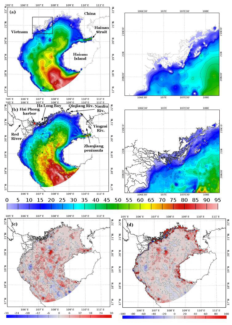
Figure 1(a, left) GEBCO bathymetry (in meters) and (a, right) details of the Ha Long Bay area (black rectangle in a, left). (b, left) TONKIN_bathymetry dataset merged with TONKIN_shorelines over GoT and (b, right) zoomed in on the Ha Long Bay area. (c) Absolute (in meters) and (d) relative (in percent) differences between TONKIN_bathymetry and GEBCO bathymetry (in meters).
The GoT is subjected to the Southeast Asian subtropical monsoon climate (Wyrtki, 1961), and therefore largely influenced by seasonal water discharges from the Red River (Vietnam) and by many smaller rivers such as the Qinjiang, Nanliu, and the Yingzai rivers (China). The Red River, which brings in average 3500 m3 s−1 (Dang et al., 2010) of water along 150 km of coastline, was ranked as the ninth river in the world in terms of sediment discharge in the 1970s with 145–160 Mt yr−1 (Milliman and Meade, 1983). Its sediment supply was drastically reduced since then to around 40 Mt yr−1 of sediment (Le et al., 2007; Vinh et al., 2014). The Red River area accounts for the most populated region of the GoT, with an estimated population of 21.13 million in 2016, corresponding to an average population density of 994 inhabitants per square kilometer (from the General Statistics Office, Statistical Yearbook of Vietnam, 2017). This region is also a key to the economy of Vietnam, with Ha Long Bay (a UNESCO world heritage site) for its particular touristic value, and with the Hai Phong port system, connecting the north of the country to the world market. This latter is the second biggest harbor of Vietnam, with a particularly fast growth rate in terms of volume of cargo passing through the port, of about 4.5×10⁶ to 36.3×10⁶ t from 1995 to 2016, respectively (Statistical Yearbook of Vietnam, 2017). However, the harbor of Hai Phong is currently affected by an increasing siltation due to tidal pumping, related to changes in water regulation by dams since the late 1980s. Such phenomenon forces a dredging effort to be more and more important each year, with USD 6.6 million spent on dredging activity in 2013 (Lefebvre et al., 2012; Vietnam maritime administration, 2017). In this particular case, fine-scale tidal modeling is of great interest for harbor management and risks prevision.
The tides in the SCS and in the GoT have been extensively studied since the 1940s (Nguyen, 1969; Ye and Robinson, 1983; Yu, 1984; Fang, 1986). Skimming through the literature, a lot of discrepancies exist in the cotidal charts before the 1980s, especially over the shelf areas. With the development of numerical models, the discrepancies have been significantly reduced by improving the accuracy of tides and tidal currents prediction.
Wyrtki (1961) was the first to identify the main tidal constituents in the SCS (O1, K1, M2, and S2), and Ye and Robinson (1983) were the first to successfully simulate the tides in the area. Until recently, only a few numerical studies have focused on the GoT (Fang et al., 1999; Manh and Yanaki, 2000; van Maren and Hoekstra, 2004) and on the Hainan Strait (Chen et al., 2009). By using, for the first time, a high-resolution model (ROMS at 1/25∘) and a combination of all available data, Minh et al. (2014) gave an overview of the dominant physical processes that characterize the tidal dynamics of the GoT, by exploring its resonance spectrum. This study improved the existing state of the art in numerically reproducing the tides of the GoT; however it also showed the limitations of using a 3D model to represent the tidal spectrum. Indeed, large discrepancies between the model and observations especially for the M2 harmonics and for the phase of S2 were found. The authors explained those discrepancies by the lack of resolution in the coastal areas due to limitations implied by the use of a regular grid and a poorly resolved bathymetric dataset.
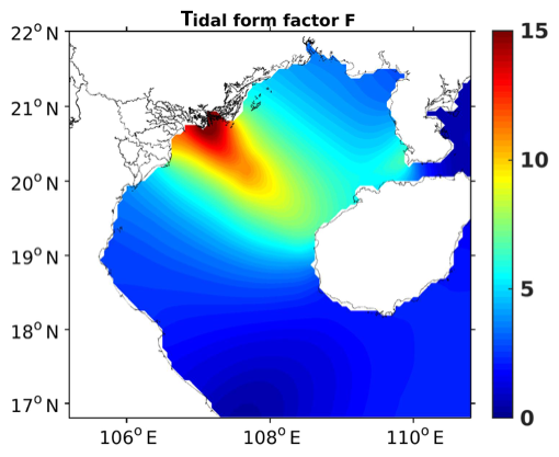
Figure 2Map of tidal form factor F computed with the amplitudes of tidal waves O1, K1, M2, and S2 obtained from FES2014b-with-assimilation. The range corresponds to semidiurnal regime, corresponds to mixed primarily semidiurnal, corresponds to mixed primarily diurnal, and F>3 corresponds to diurnal regime.
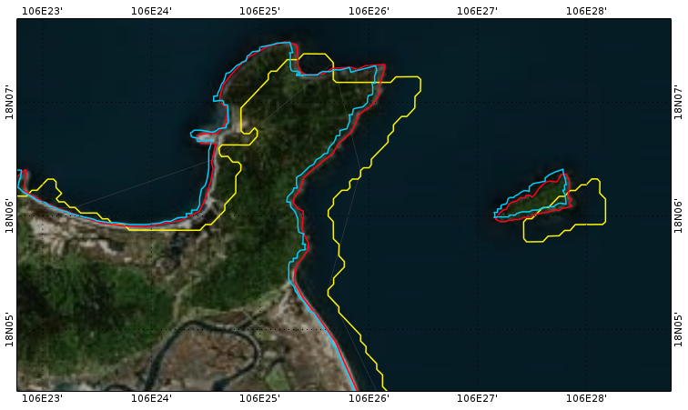
Figure 3Shoreline products from OpenStreetMap (blue line), GSHHG (yellow line), and TONKIN_shorelines (red line) superimposed on a satellite image downloaded from Bing (© Bing™) over a small region of the GoT.
The SCS and the GoT are some of the few regions in the world where diurnal tides dominate the semidiurnal tides (Fang, 1986). The tidal form factor (F), or amplitude ratio, defined by the ratio of the amplitude of the two main diurnal over the semidiurnal constituents, as , provides a quantitative measure of the general characteristics of the tidal oscillations at a specific location. If , then the regime is semidiurnal, if , the regime is mixed primarily semidiurnal, if , the regime is mixed primarily diurnal, and if F>3, the regime is diurnal. Values of F shown in Fig. 2 are calculated using tidal amplitudes from FES2014b-with-assimilation (product described in Sect. 2.2.3). At the entrance of the GoT and at the Hainan Strait, the tides are defined as mixed primarily diurnal, with F varying from 1.5 and 2.2 depending on the given locations. At the Red River Delta, F is around 15, attesting to a diurnal regime. Indeed, the major branch of energy flux entering the basin from the southwest is weak for the semidiurnal tides and strong for the diurnal ones. A second branch of energy (also diurnal tidal waves) enters the GoT through the Hainan Strait (Ding et al., 2013).
In coastal seas and bays, tides are primarily driven by the open ocean tide at the mouth of the bay. By resonance of a constructive interference between the incoming tide and a component reflected from the coast, a large tide amplitude can be generated. In the GoT case, tidal waves enter the basin from the adjacent SCS, and due to the basin geometry, O1 and K1 resonate (Fang et al., 1999). Their amplitudes reach 90 and 80 cm respectively. The Coriolis force deflects the incoming waves to the right and pushes them against the northern enclosure of the basin. Once the waves are reflected, they propagate southward until they slowly dissipate by friction. Fang (1999) found that the amplitude of the tide gradually decreases from 4 to 2 m north to south during spring tide. The amplitude of O1 in the GoT is larger than K1 because of a larger resonance effect, even though its amplitude in the SCS is smaller than K1 (Minh et al., 2014). The largest semidiurnal waves of the GoT are M2 and S2. They both appear as a degenerated amphidrome with smallest amplitudes near the Red River Delta in the northwestern head of the Gulf (between 5 and 15 cm for M2 and below 5 cm for S2) (Hu et al., 2001). Given those values of amplitude, Van Maren et al. (2004) defined the tidal regime in the GoT as mesotidal and locally even macrotidal, even though diurnal tidal regimes are usually mainly microtidal.
Our first objective in this paper is to propose a robust and simple approach that allows the quantification of the sensitivity of the tidal solutions to bottom friction parameterization and to bathymetric changes in the Gulf of Tonkin. This article furthermore represents the first step in a more comprehensive modeling study aiming at representing the transport and the fate of sediments from the Red River to the Gulf of Tonkin using the tridimensional structured coupled SYMPHONIE–MUSTANG model (Marsaleix et al., 2008; Le Hir et al., 2011). In this framework, our final objective is to optimize the configuration (bathymetry) and parameterization (bottom stress) that will be used in this forthcoming study. These objectives are based on the quantification of the response of the tidal solutions to the calibration of the bottom friction and to the improvements in the bathymetry.
As evidenced by Fontes et al. (2008) and Le Bars et al. (2010), local tidal simulations are mainly affected by the bathymetry and the bottom stress parametrization. These latter often lack of details in remote coastal regions and/or in poorly sampled regions (in terms of bathymetry and tide gauges). It is particularly the case for the GoT. By its location at the boundary between China and Vietnam and by its intense maritime transport activity, the region is extremely difficult to sample, in particular in the highly protected region of Ha Long Bay, in the Hainan Strait, and in the nearshore/coastal areas. In situ data and soundings are consequently rare and yet extremely valuable. The precise goal of the present study is therefore to build an improved bathymetry and coastline database over the GoT and to define the best configuration for bottom stress parameterization in this region, evaluating the impact of those parameters on the tidal representation in the GoT. The resulting optimized configuration will then be used for future numerical studies of ocean dynamics and sediment transport in the region. For that, we first worked on the improvement in the general and global bathymetric datasets available, i.e., GEBCO (Monahan, 2008), the Smith and Sandwell bathymetry (Smith and Sandwell, 1997), and the ETOPO1 Global Relief Model (Amante and Eakins, 2009), by incorporating new sources of data. We then worked on the optimization of the bottom stress parameterization. Our approach to addressing the issue of the parametrization and to evaluating the impact of our configuration setup is based on the use of the hydrodynamical model T-UGOm model of Lyard et al. (2006). Thanks to its frequency-domain solver, shortly described in the next sections, T-UGOm can indeed perform tidal simulations at an extremely limited computational cost (compared to time-stepping solver), in our case roughly 80 times faster than usual time-stepping hydrodynamical models (i.e., from a few minutes for T-UGOm compared with hours/days). Furthermore, different formulations for the bottom friction can be prescribed along with a varying spatial distribution of its related parameters (roughness or friction factor). These particular assets allow a large number of sensitivity tests to be performed at a reasonable computational cost on bathymetric and bottom stress parametrization, hence speeding up the processes of precise tuning and calibration/validation of our configuration.
In Sect. 2, we describe the bathymetry, shorelines and waterways construction as well as the numerical model and the modeling strategy in terms of sensitivity experiments. The data used for model evaluation and the metrics used for this evaluation are also presented in this section. In Sect. 3 we present the results regarding the sensitivity of simulations to bottom stress parametrization and to bathymetry. Conclusions and outlook are given in Sect. 4.
2.1 Shorelines and bathymetry construction
The first step of our work is to improve the shoreline and bathymetry precision. Two global digital shorelines are commonly used for representing the general characteristics of the GoT shorelines: the Global Self-consistent, Hierarchical, High-resolution Geography Database (GSHHG, Wessel and Smith, 1996) and the free downloadable maps from OpenStreetMap (OpenStreetMap contributors, 2015; retrieved from http://www.planet.openstreetmap.org, last access: 20 May 2018). The GSHHG and OpenStreetMap shoreline products are both superimposed on satellite and aerial images of the GoT downloaded from Bing (https://www.bing.com/maps, last access: 15 June 2018) and used now as our reference. Bing is chosen here for the accessibility of its open data, which makes our shoreline construction method doable by everyone. Figure 3 shows the shoreline products superimposed on a downloaded image of a small region of the GoT. When closely comparing the shoreline products to the images, it appears that the OpenStreetMap product looks fairly reasonable all along the coastlines of the GoT, except in the Ha Long Bay area (not shown) where the complex topography and the islets are clearly too numerous. However, the OpenStreetMap shoreline is most of the time shifted by a few meters westwards compared to the land (Fig. 3). The GSHHG dataset suffers from the same problem but shifted by up to 500 m eastwards. The observed shifts in both OpenStreetMap and GSHHG products are not documented but could be due, among other things, to the use of nautical charts and/or local topography maps for product construction, which could have been collected before accurate GPS measurements in the area. Our objective in this study is to propose a grid matching the reality (i.e., Bing maps, our reference) as close as possible; therefore, none of these databases looked precise enough to meet our expectations. Consequently, we have built our own shorelines dataset, named TONKIN_shorelines, by using the POC Viewer and Processing (POCViP) software (available on the CNRS sharing website, https://mycore.core-cloud.net/index.php/s/ysqfIlcX5njfAYD/download, last access: 9 December 2019), developed at LEGOS. The satellite and aerial images of the region, previously downloaded from Bing, are georeferenced with POCViP. The software allows the user to draw nodes and segments with a resolution as fine as needed. The resulting TONKIN_shorelines database has a resolution down to 10 m, and its accuracy is observable in Fig. 3. We followed the same procedure for building a waterways database of the Red River system. This latter is also included in TONKIN_shorelines. For the Ha Long Bay area, another strategy has been considered since drawing by hand each islet would have been unaffordably time consuming. In this case, images from the Shuttle Radar Topography Mission (SRTM) (https://earthexplorer.usgs.gov/, last access: 2 July 2018) were downloaded and coastlines got extracted and merged with TONKIN_shorelines.
Because of the shallowness of the area, the bathymetry of the GoT is a critical point and could have a strong impact on tidal simulations as it is often the main constraint in tidal propagation (Fontes et al., 2008). The GEBCO 2014 (30 arcsec interval grid) dataset is largely based on a database of ship-track soundings, whose resolution can be locally much finer than 1 km, but gridded data are provided with a ∼ 1 km resolution (as explained on the GEBCO website: https://www.gebco.net/data_and_products/historical_data_sets/ (last access: 16 November 2019). The GEBCO dataset can hence be used to represent the slope and the shape of the basin at a relatively large scale (Fig. 1a, b). However, this 1 km resolution is too low to accurately represent detailed geomorphological features, in particular in coastal regions, near the delta, and in the Ha Long Bay area. For the purpose of providing an improved tidal solution, we have developed a bathymetry with a better precision, named TONKIN_bathymetry (Fig. 1c, d). For that, we have merged the GEBCO bathymetry with digitalized nautical charts of type CM-93 via OpenCPN (https://opencpn.org/, last access: 20 July 2018). Note that bathymetric data from nautical charts in coastal shallow areas are often chosen to be shallower than the real bathymetry for navigation security purposes. We also incorporated the tidal flats digital elevation model from Tong (2016). This author used waterlines from Landsat images of 2014 to construct a surface model from elevation contours. As tidal flats are suffering from a tidal regime with submersion during flood tide and exposure during ebb tide, their representation is crucial in tidal modeling. TONKIN_bathymetry is merged with TONKIN_shorelines dataset.
This scattered bathymetric dataset shows realistic small-scale structures and depths over the shelf and in the Ha Long Bay area. The details and the islets of the bay are now represented (Fig. 1c, d), as well as the Red River waterways. In the deeper part of the basin, near the boundary, two deeper branches (in light red) are distinguishable. These latter could correspond to the location of the ancient river bed of the Red River during the last glacial time, which split in two around 18∘ N–108∘ E (Wetzel et al., 2017). The biggest differences compared to GEBCO are observed in the central part of the region and in the Hainan Strait (Fig. 1e, f). In the strait, the GEBCO bathymetry underestimates depths by roughly 20 m (∼ 50 % in terms of relative difference) compared to TONKIN_bathymetry. In the center, differences can be up to 30 m between the two datasets (not shown on the color bar), corresponding to relative differences of up to 100 %. Such high observed discrepancies are due to the interpolation of the scattered measuring points from the nautical charts. High relative differences are also observed all along the coastlines, corresponding for most of them to the integration of the intertidal dynamical elevation model (DEM) in the Red River Delta area, as well as to a better resolution in shallow areas obtained from the nautical charts. Discrepancies in most other parts of the basin remain roughly below 30 %. Patches of differences of about 40 % between the datasets are also observed at the open ocean boundary of the domain, with GEBCO also underestimating depths in the southernmost part.
We draw attention to the fact that the TONKIN_bathymetry dataset provides an improvement to the available bathymetric dataset but that some flaws and uncertainties still exist, partly due to sampling methods and shallower waters induced by nautical charts data.
2.2 Model, configuration and forcings
2.2.1 T-UGOm hydrodynamic model
The tidal simulations are based on the unstructured grid model T-UGOm (Toulouse Unstructured Grid Ocean Model) developed at LEGOS and is the follow-up of MOG2D (Carrère and Lyard, 2003). In its standard applications, T-UGOm uses unstructured triangle meshes allowing for an optimal grid resolution flexibility, in particular to discretize complex coastal geometry regions, to follow various local dynamical constraints, such as rapid topography changes, or to simply adapt resolution in regions of special interest. The flexibility of unstructured triangle meshes is fully adequate for fine-scale modeling, especially in delta or estuarine systems, whereas usual structured meshes may struggle to represent fine geography of certain areas. The T-UGOm model is widely used in global to coastal modeling, mostly for tidal simulations; in the representation of semi- and quarter-diurnal barotropic tides in the Bay of Biscay (Pairaud et al., 2008), in studying the tidal dynamics of the macro-tidal Amazon estuary (Le Bars et al., 2010), in the representation of tidal currents over the Australian shelves (Cancet et al., 2017), and in assessing the role of the tidal boundary conditions in a 3D model in the Bay of Biscay (Toublanc et al., 2018). Furthermore, T-UGOm has proven its accuracy in global barotropic tidal modeling in the Corsica Channel (Vignudelli et al., 2005) and in a global assessment of different ocean tide models (Stammer et al., 2014).
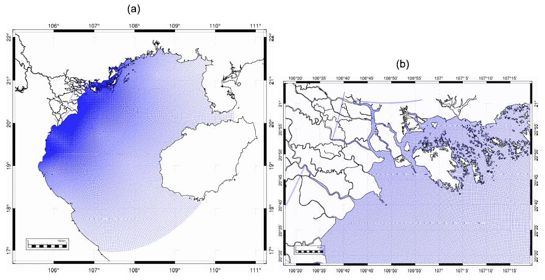
Figure 4Model mesh over (a) the GoT and (b) zoomed in on the Ha Long Bay region. The maximum refinement (150 m) is reached in the river channels.
In addition to its traditional time-stepping solver, it has the remarkable particularity to include a frequency-domain solver kernel, which solves for the 2D/3D quasi-linearized tidal equations. This spectral mode solves the quasi-linearized Navier–Stokes equations in the spectral domain, in a wave by wave, iterative process (to take into account nonlinear effects such as bottom friction). It has demonstrated its efficiency (accuracy and computational cost) for the astronomical tide simulation as well as for the nonlinear tides. The frequency-domain solver can be used either on triangle or quadrangle unstructured mesh and therefore can be used on any C-grid configuration. Compared to a traditional time-stepping mode that simulates the temporal evolution of the tidal constituents over a given period, the numerical cost of the frequency-domain mode (2D) is roughly 1000 times smaller.
For our purpose of assessing the sensitivity to various parameters of the tide representation by the model, T-UGOm is set up in a 2D barotropic, quadrangle grid, shallow-water, and frequency-domain mode (version of the code: 4.1 2616). This configuration (including TONKIN_bathymetry and the specific version of T-UGOm code) is from hereafter named TKN. The main advantage of this fast and reduced-cost solver is the possibility to perform in an affordable time a wide range of experiments at the regional or global scale, in order to parameterize the model, such as the following: optimize bottom stress parametrization, test bathymetry improvements, and other numerical developments. In our case, the run duration of a spectral simulation with T-UGOm lasts on average 6 min (CPU time), which is roughly 40 times quicker than a simulation with a regional circulation model such as SYMPHONIE (Marsaleix et al., 2008; CPU time is approximately 4 h for a 9-month simulation, corresponding to the required time with SYMPHONIE to separate the tidal waves).
Another useful functionality of T-UGOm for our study is the possibility to locally prescribe the bottom friction, including the roughness length and also the choice of parametrization type. In some shallow coastal regions like the GoT, the presence of fluid mud flow and fine sediments can induce dramatic changes on bottom friction. The quadratic parameterization may be obsolete, and a linear parameterization may be more adequate (Le Bars et al., 2010) and will be tested hereafter. This functionality is essential in those particular regions like shallow estuaries, where the influence of bottom friction on the tides propagation is crucial.
2.2.2 Numerical domain over the GoT
The numerical domain over the GoT, built from the TONKIN_bathymetry, is discretized on an unstructured grid made of quadrangle elements (Fig. 3). The most commonly used elements in T-UGOm are triangles; however here the final goal of our work is to use the resulting grid for coupled hydrodynamical–sediment transport models like SYMPHONIE–MUSTANG using quadrangle structured C-grids. We therefore run the T-UGOm tidal solver on a quadrangle grid. As in Madec and Imbard (1996), this grid is semi-analytical. A first guess is provided by the analytical reversible coordinate transformation of Bentsen et al. (1999), which produces a bipolar grid. The singularities associated with the two poles are located in the continental mask, slightly to the north of the numerical domain, where the horizontal resolution is the strongest (Fig. 4). This first guess is then slightly modified to control the extension of the grid offshore, in practice to prevent extension beyond the continental shelf. As in Madec and Imbard (1996) this second stage is partly numerical (and preserves the orthogonality of the axes of the grid). The largest edges of the quadrangles are about 5 km at the boundaries of the domain and the smallest are about 150 m long, with a maximum refinement located in the river channels (Fig. 5). This grid allows the complexity of the islets of Ha Long Bay as well as the details of the coastlines of the Red River Delta to be represented. A regular C-grid would hardly take into account such complex topography and details.

Figure 5O1 tidal amplitude (in meters) from different products: (a) FES2014b-with-assimilation, (b) FES2014b-without-assimilation, (c) TKN-gebco, and (d) TKN. The circle diameter is proportional to the complex error (Appendix; Eq. A2) between the solutions and satellite altimetry (in meters). The colored circles denote the amplitude of O1 harmonic measured at the corresponding tide gauge station.
2.2.3 Tidal open-boundary conditions
For modeling barotropic tidal waves, nine tidal constituents have been imposed as open boundary conditions (OBCs) in elevation (amplitude and phase) for our domain: O1, K1, M2, S2, N2, K2, P1, Q1, and M4. Since the astronomical spectrum of tide is dominant in the GoT, eight out of the nine constituents simulated are astronomical constituents, and M4 is chosen here as a representative of all nonlinear interactions. These constituents, ordered by their amplitudes (in the GoT), are the main tidal waves in the GoT and come from the FES2014b global tidal model resolved on unstructured meshes but distributed on a resolution-coherent grid. FES2014b (Carrère et al., 2016) is the most recent available version of the FES (finite element solution) global tide model that follows the FES2012 version (Carrère et al., 2012). The FES2014b global tidal atlas includes 34 tidal constituents and is based on the resolution of the tidal barotropic equations with T-UGOm (frequency-domain solver for the astronomical tides and time-stepping solver for the nonlinear tides, described in the above section). The FES2014b bathymetry has been constructed from the best available (compared to previous FES versions) global and regional DTMs (dynamical topography models) and corrected from available depths soundings (nautical charts, ship soundings, and multibeam data) to get the best possible accuracy, typically 1.3 cm RMS (root-mean-square error) for the M2 constituent in the deep ocean before data assimilation. The tidal simulation performed using this configuration and without assimilation is called FES2014b-without-assimilation. Moreover, in addition to the hydrodynamic solutions, data-derived altimetry and tide gauges harmonic constants have been assimilated, using a hybrid ensemble/representer approach, to improve the atlas accuracy for 15 major constituents and fulfill the accuracy requirements in satellite ocean topography correction. This version of FES will from hereafter be named FES2014b-with-assimilation in the following, in comparison to FES2014b-without-assimilation. Thanks to the accuracy of the prior FES2014b-without-assimilation solutions and the subsequent higher efficiency of data assimilation, this latest FES2014b-with-assimilation version of the FES2014 atlas has reached an unprecedented level of precision and has shown accuracy that is superior to any other previous versions (see http://www.aviso.altimetry.fr/en/data/products/auxiliary-products/global-tide-fes.html, last access 15 June 2018; Florent Lyard, personal communication, 10 October 2018).
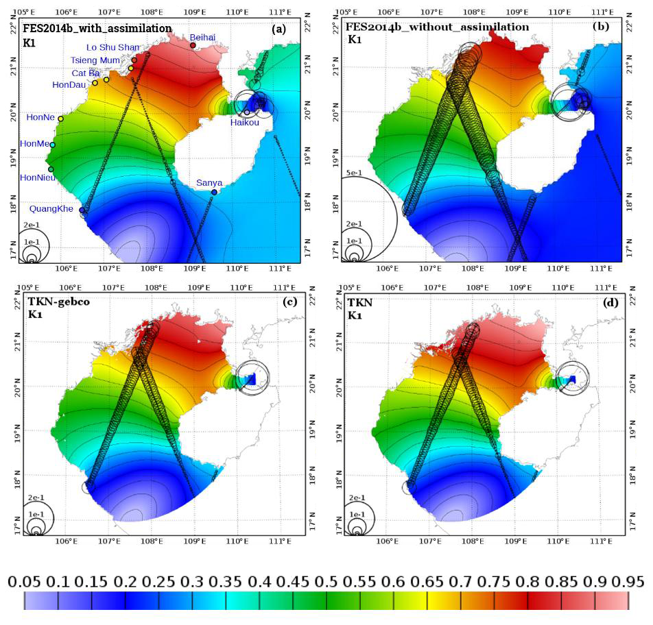
Figure 6Same as Fig. 5 for K1.
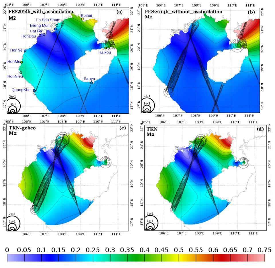
Figure 7Same as Fig. 5 for M2.
The tidal distribution of the O1, K1, M2, and S2 tidal waves and their first harmonics from FES2014b-with-assimilation and FES2014b-without-assimilation is shown in Figs. 4a, b, 5a, b, 6a, b, 7a, and b, as well as their error along the satellite altimetry track dataset of CTOH-LEGOS (described below in Sect. 2.3.1). FES2014b-with-assimilation shows negligible errors compared to FES2014b-without-assimilation thanks to the assimilation. The main interest of using FES2014b-without-assimilation in our study is to assess the real capacity of the FES model to reproduce the tidal harmonics without using data assimilation, whereas FES2014b-with-assimilation can be used together with satellite altimetry as a reference to evaluate tidal solution errors.
The T-UGOm code, the model grid, and the configuration files used for our simulations are available in Zenodo/Piton (2019a–c; see Code and data availability section).
2.3 Simulations and evaluation
We use the model configuration described above to assess the impact of the improvement in our bathymetry database and to optimize the representation of bottom friction in the model. For that we perform sensitivity simulations that we compare with available data using specific metrics. Those tools and methods are presented in this section.
2.3.1 Modeling strategy and sensitivity experiments
The T-UGOm 2D model (in its frequency-domain, iterative mode) is run on the high-resolution grid described in Sect. 2.2.2. The following sections describe the tests performed for the bottom friction parametrization.
Bottom stress parametrization
In shallow areas where current intensities are strong due to a macro-tidal environment combined with strong rivers flows and winds forcing, the sensitivity of the model to the bottom stress is significant. The bottom stress is thus a crucial component for modeling nearshore circulation and sediment transport dynamics (Gabioux et al., 2005; Fontes et al., 2008). The bottom stress formulation depends upon a nondimensional bottom drag coefficient (or friction coefficient) CD and can be obtained, in barotropic mode, as follows:
with the depth averaged velocity and ρ the fluid density.

Figure 8Same as Fig. 5 for S2.
In this study, we test two commonly used parameterizations: a constant drag coefficient CD assuming a constant speed profile and a drag coefficient CD depending upon the roughness height z0.
In the first parameterization, a constant profile of the speed is assumed over the whole water height, leading to quadratic bottom stress and a constant CD that depends on the Chézy coefficient C and on the acceleration due to gravity g (Dronkers, 1964) as follows:
In the second parameterization, a logarithmic profile of the speed is assumed over the whole water column (Soulsby et al., 1993), leading to a CD depending upon the roughness length z0, the total water height H, and the von Kármán's constant κ=0.4 as follows:
The roughness length z0 (also called roughness height) depends on not only the morphology of the bed (i.e., the presence of wavelets or not) but also the nature of the bottom sediment. In presence of fluid mud, the friction is considered as purely viscous (Gabioux, 2005). However, the repartitioning of sediments and the structure of the seabed are not uniform over the GoT shelf as the Red River discharge causes patches of sediments of different natures (Natural Conditions and Environment of Vietnam Sea and Adjacent Area Atlas, 2007). Consequently, we can expect z0 to vary spatially. This issue can be addressed with T-UGOm since it contains a domain partition algorithm allowing it to take into account the spatial variability in the seabed roughness. Furthermore, this CD parameterization, which includes a logarithmic profile of the speed, allows the adaption of CD to the model vertical resolution by considering the water column depths, as a way to correspond to the friction coefficient resolution in 3D models.
In the case of fluid mud when the bottom friction is purely viscous and the velocity profiles are linear, Gabioux et al. (2005) described the τb as follows:
with r corresponding here to the friction coefficient.
A third parameterization of the coefficient of friction is tested in this study; a linear profile of the speed is assumed over the whole water column, which characterizes viscous conditions. In this case, a linear bottom stress is assumed, and r depends on the frequency of the forcing wave ω (here O1) and the fluid kinematic viscosity v as follows:
In this study, these three formulations of the coefficient of friction (Eqs. 2, 3, and 5) are tested for model parameterization, varying, respectively, the value of CD, the value of z0, and the value of r.
Sensitivity to uniform friction parameters
Sensitivity numerical experiments were first conducted in order to assess the sensitivity of the model to uniform parameters of friction for two of the parameterizations described above, which include a quadratic bottom stress with a uniform drag coefficient CD (i.e., CD= constant) (Eqs. 1 and 2) and a logarithmic variation in CD depending on a uniform bottom roughness height z0, i.e., (Eq. 3). For that, we performed a first set (SET1) of 45 tests, running the model with a constant CD with CD values spanning from to m (see Fig. 9 where we plotted CD values spanning from 0.5 to m). We then performed a second set (SET2) of six tests running the model with a by testing values from to m for z0 (see Fig. 10).
Sensitivity to the regionalization of the roughness coefficient
As mentioned in the previous section, a uniform roughness coefficient does not usually allow for reaching a satisfying level of accuracy over the whole domain, since the variability in the seafloor morphology is not fully taken into consideration. To take this variability into account, the spatial variability in the seabed roughness must be prescribed to the model. For that, our study area is divided into several zones based on seabed sediment types repartition obtained from the Natural Conditions and Environment of Vietnam Sea and Adjacent Area Atlas (2007).
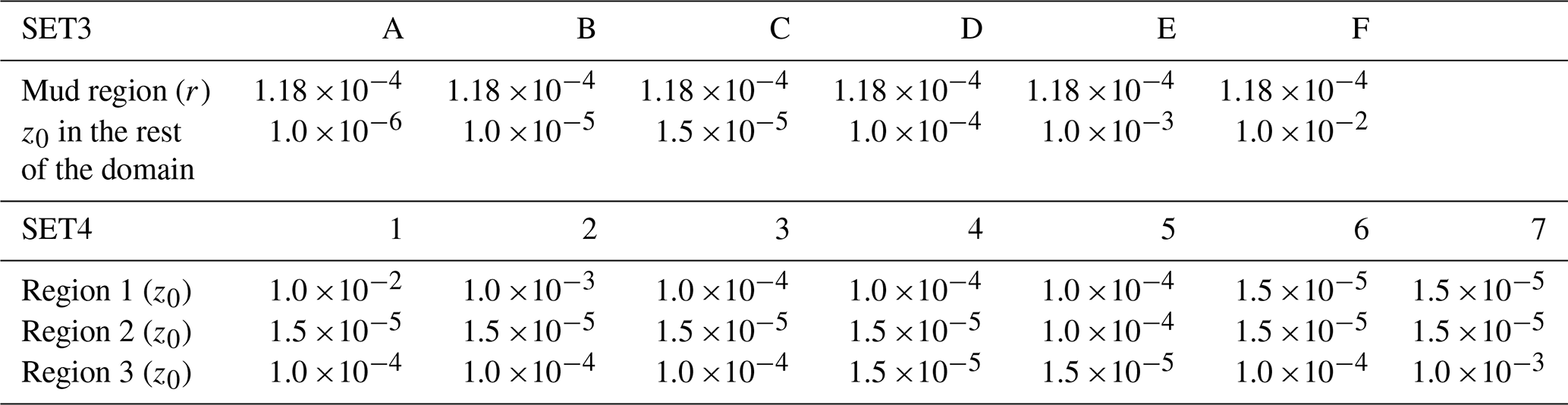
The third set of sensitivity experiments (SET3, Tests A to E in Table 1) consisted of prescribing a linear velocity profile only in the area of fine mud, following Eqs. (4) and (5), with a fixed m (see Fig. 10a), and testing different values of uniform z0 (from to m) over the rest of the region, prescribing a logarithmic velocity profile. This value of r is taken from the value empirically tuned on the region of the Amazon estuary and shelf with the configuration described in Le Bars et al. (2010).
The fourth set of sensitivity experiments (SET4, Tests 1 to 7 in Table 1) consisted of dividing the region into three zones, according to a supposed spatial distribution of the seabed sediments, inspired from the above-mentioned Vietnamese atlas (Fig. 12b), as follows: zone 1 is mostly composed of muddy sand, zone 2 is composed of mud, and zone 3 is composed of sand and coarser aggregates. In each zone, a value of z0 (from to m) is prescribed following a (Eq. 3). Note that for this set of experiments every combination of z0 was tested, yet for the sake of clarity we show and describe in Sect. 4 only the ones with errors (see Sect. 2.3.3) for S2 solutions below 2.5 cm.
The fifth and last set of experiments (SET5) consisted of dividing the domain into 12 zones, in order to refine the representation of the spatial distribution of the sediments of the seafloor following the Vietnamese atlas (Fig. 12c). Zones 1 and 11 correspond to muddy sand, zones 2, 6, 10, and 12 correspond to slightly gravelly sand, zones 3 and 5 correspond to sandy mud, zone 4 corresponds to fine mud, zone 7 corresponds to sandy gravel, zone 8 corresponds to slightly gravelly mud, and zone 9 corresponds to sand. Different z0 values (varying from to m), using , were prescribed to each of the 12 zones, and the corresponding runs were performed, each time imposing a random and different value to each zone.
2.3.2 Satellite data and tide gauges data for model assessment
The evaluation of the performance of the simulations is made with along-track tidal harmonics obtained from a 19-year-long (1993–2011) time series of satellite altimetry data available every 10 d from TOPEX/Poseidon (T/P), Jason-1, and Jason-2 missions (https://doi.org/10.6096/CTOH_X-TRACK_Tidal_2018_01). These data are provided by the CTOH-LEGOS (Birol et al., 2016). The tracks of the altimeters passing over the GoT are shown in Figs. 5–8 and are spaced by approximately 280 km. To complement those data in the inter-track domain, we also compare our simulations with the FES2014b-with-assimilation tidal atlas, as explained in Sect. 2.2.3.
Harmonic tidal constituents at 11 tide gauge stations are also used for evaluation of the simulations. The data are distributed by the International Hydrographic Organization (https://www.iho.int/, last access: 2 November 2019) and are available upon request at https://www.admiralty.co.uk/ukho/tidal-harmonics (last access: 2 November 2019). The name and position of these stations are shown in Fig. 5a. Amplitudes and phases of O1, K1, M2, and S2 at the 11 gauge stations are available in Chen et al. (2009).
2.3.3 Metrics
For comparison of the simulations with the tidal harmonics from satellite altimetry, two statistical parameters (metrics) are used. These are the root-mean-square error (RMS*) and the mean absolute error (MAE). The RMS* computation is based on a vectorial difference, which combines both amplitude error and phase error into a single error measure. The errors computations are detailed in the Appendix.
In this section we present the results concerning the sensitivity of the modeled tidal solutions to the choice of bathymetry dataset and to the choice of bottom friction parameterization. Spatially varying uniform friction parameters only slightly improve the tidal solutions compared to uniform parameters. Furthermore, prescribing a linear parameterization in supposed fluid mud areas does not allow a significant improvement in the solutions, unlike in Le Bars et al. (2010). Lastly, the reconstructed bathymetry dataset allows the semidiurnal tidal solutions to be strongly improved. The improvements consist mainly of a correction near the coasts and of reducing the errors in phase (as can be expected from a bathymetry upgrade). We present the results of the conducted sensitivity experiments in detail in the following subsections.
.
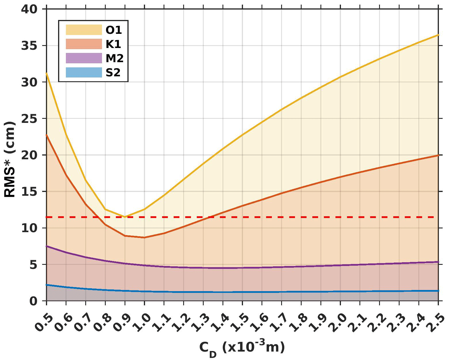
Figure 9Model complex errors (Appendix; Eq. A2) relative to altimetry along-track data for tests performed with varying the values of the uniform drag coefficient CD over the domain (SET1). The space in between two lines corresponds to the error for each wave. The yellow line therefore corresponds to the cumulative error for all four waves. The dashed red line corresponds to the smallest cumulative error, here equal to 11.50 cm and obtained for m
3.1 Model sensitivity to bottom stress parameterization
3.1.1 Sensitivity to a constant or varying CD (SET1 and SET2)
We first analyze in this section and in the next one the sensitivity to the parameterization of bottom friction. Firstly, to show the sensitivity to the choice of uniform friction parameters, the model errors (Appendix; Eq. A2) compared to satellite altimetry are shown in Fig. 9 (SET1) and Fig. 10 (SET2), for the main tidal constituents (O1, K1, M2, and S2) for each value of uniform CD and z0 tested in SET1 and SET2, described in Sect. 2. On both Figs. 9 and 10, the space in between two solid lines corresponds to the errors for the considered wave (see legend), and the yellow line represents the cumulative errors for the four waves. The dashed red line represents the smallest cumulative error (i.e., the minimum value reached for the yellow line).
First of all, the diurnal waves O1 and K1 are more affected by the changes in the values of CD and z0 than the semidiurnal waves M2 and S2 (Figs. 9 and 10). This can be explained by the fact that diurnal tides are of greater amplitude than semidiurnal tides in the Gulf of Tonkin; thus the tidal friction is truly nonlinear for O1 and K1 and marginally only for M2 and S2. For CD values below 0.6 and above m, O1 and K1 errors are larger than errors for M2 and S2. For example, for m the errors for O1 are roughly 4 to 11 times larger than errors for M2 and S2, and errors for K1 are roughly 3 to 10 times larger than errors for M2 and S2, respectively.
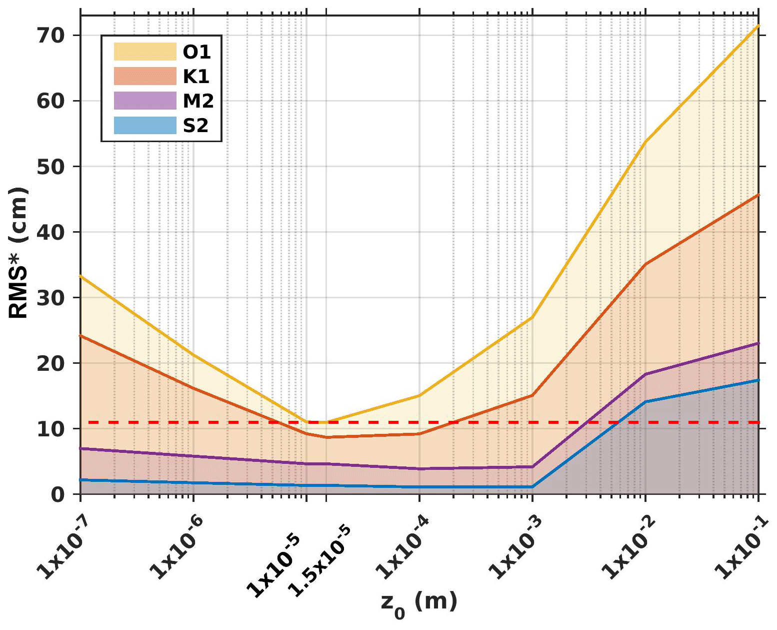
Figure 10Model complex errors (Appendix; Eq. A2) relative to altimetry data for tests performed with varying the values of the uniform z0 over the domain (SET2). The space in between two lines corresponds to the error for each wave. The yellow line corresponds to the cumulative errors for all four waves. The dashed red line corresponds to the smallest cumulative error, here equal to 10.96 cm and obtained for m.
Small values of CD also induce large errors of O1 and K1 (for m, errors for O1 are roughly 1.5 to 3.8 times larger than errors for M2 and S2, and errors for K1 are roughly 2.8 to 6.9 times larger than errors for M2 and S2, respectively). High and small values of z0 also trigger larger errors in the diurnal waves (Fig. 10).
Secondly, the tests of sensitivity to a spatially constant friction coefficient CD show that the lowest error is reached for m (the cumulative error is equal to 11.50 cm) (Fig. 9). This value of CD is roughly half as low as those used for the whole South China Sea ( m: Fang et al., 1999; Cai et al., 2005) and similar to the one used in the GoT by Nguyen et al. (2014) of m. The tests of sensitivity to the roughness length z0 show that the value m yields the least errors (the cumulative error is equal to 10.96 cm) (Fig. 10). This is a relatively small roughness length value, indicating a seabed composed of very fine particles. Finally, the use of a constant CD parametrization with a CD of m or a constant roughness length with a z0 of m leads to almost identical errors (0.54 cm of difference). The similarity of the results between the two simulations is due to the values of CD obtained for m; those values vary spatially from 0.8 to m and are thus very close to the optimized value of m for a constant CD (figure not shown). This small spatial variability in the varying CD explains why the results of the two optimized simulations from SET1 and SET2 are finally similar.
The rather low values of friction ( m) and roughness coefficients ( m) suggest the presence of a majority of fine sediments in the GoT. This is consistent with the results from Ma et al. (2010), who found the western and central parts of the GoT to be mainly composed of fine to coarse silts, with a few patches of sand next to Hainan Island.
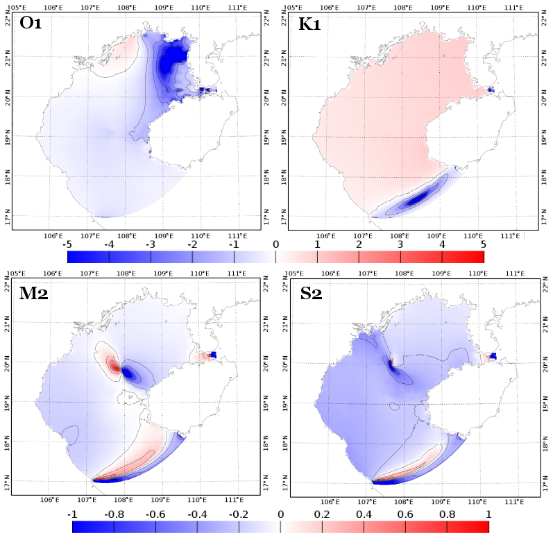
Figure 11Relative differences (in percent) between simulation with ) and simulation with m compared to FES2014b-with-assimilation (as a reference) for the tidal harmonics of O1, K1, M2, and S2.
Thirdly, the lowest error for each wave is reached for different values of CD and z0. In SET1, the lowest error value for O1 is reached when m, while the lowest error value for K1 is reached for m. The lowest errors values of the semidiurnal waves are reached for m (Fig. 9). In SET2, the lowest errors values of the diurnal waves are reached for m and are reached for m for the semidiurnal waves (Fig. 10). This finding is of course unphysical, and the reader must keep in mind that optimal parameter setting also often deals with model errors numerical compensation. In our study, it is quite obvious that the model bathymetry is far from perfect despite the large efforts carried out to improve the topographic dataset, and remaining errors due to bathymetry imperfections can be partly canceled by the use of an adequate (i.e., numerical, not physical) friction parameter. As bathymetry-induced errors will be strongly affected by the tidal frequency group (species) and since bathymetry directly and distinctly impacts phase propagation of the waves, we can expect that optimal friction parameterization alteration (and corresponding alterations of the bottom shear stress) will slightly vary in a given frequency group but strongly from one to another. The examination of sensitivity studies tends to promote the idea that these differences are mostly due to remaining errors in the bathymetric dataset, and the final decision for an optimal friction parameterization will be based on the best compromise for the overall solution errors. As the K1 and O1 sensitivity to friction alteration is prevailing, the compromise is of course mostly driven by these two tidal waves.
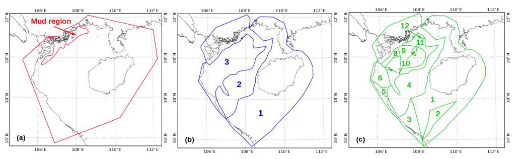
Figure 12Spatial partitioning of the domain for the set of experiment SET3 (a), for SET4 (b), and for SET5 (c).
To assess the significance of the differences between two parameterizations, Fig. 11 presents spatially the relative differences between the two simulations (SET1 and SET2), in terms of performance in amplitude and phase, taking FES2014b-with-assimilation as a reference. Negative values (in blue) indicate that the simulation from SET2 with a z0 of m produces the smallest differences in the reference, while positive values (in red) indicate that the simulation from SET1 with a constant CD of m produces the smallest differences in the reference. For K1, values are positive over almost all of the GoT basin, indicating that the tidal solution from simulation with a constant CD (SET1) performs better. However the differences in performance between the two simulations are very small, ∼ 0.5 %. For O1, M2, and S2 cases, values are mostly negative over the GoT, suggesting that simulation with a z0 of m (SET2) better represents the tidal solutions for these three waves than simulation with a constant CD (SET1). Once again, however, these improvements are really small (lower than 5 %). These results finally show that the tidal solutions are not very sensitive to changes in bottom friction parameterization, from a constant CD to a CD varying with z0.
3.1.2 Sensitivity to the value of spatially varying roughness length (SET3, SET4, and SET5)
The results of the tests performed to assess the model sensitivity to a regionalized roughness coefficient (see Table 1) are shown in Fig. 13.
Sensitivity to a quadratic or linear stress (SET3 vs. SET2)
No significant improvement in the tidal solutions is obtained from SET3, i.e., by imposing a linear flow in the mud region (where the resolution is the highest), compared to the tests performed with spatially uniform parameters (drag coefficient, SET1 and bottom roughness length, SET2, Figs. 9 and 10). The cumulative error of all four waves (yellow line) is always above the 10.96 cm value of the smallest error found for SET2 (the smallest cumulative error of 11.33 cm is obtained for Test C). Results from SET3 (Tests A to F) show that the solutions still greatly depends upon the roughness length values imposed on the rest of the region, with errors increasing with low and high values of z0; from Tests D to G, cumulative errors increase by a factor 3.5 with z0 values increasing from to m; from Test A to B, errors decrease by a factor of 2, with values decreasing from to m. As previously observed, the diurnal waves O1 and K1 (in Tests A to F) are more sensitive to changes in z0 than the semidiurnal M2 and S2 waves; for m, errors of O1 are 3 and 7 times larger than errors of M2 and S2, respectively, and errors of K1 are 4.5 to 11 times larger than errors of M2 and S2, respectively.
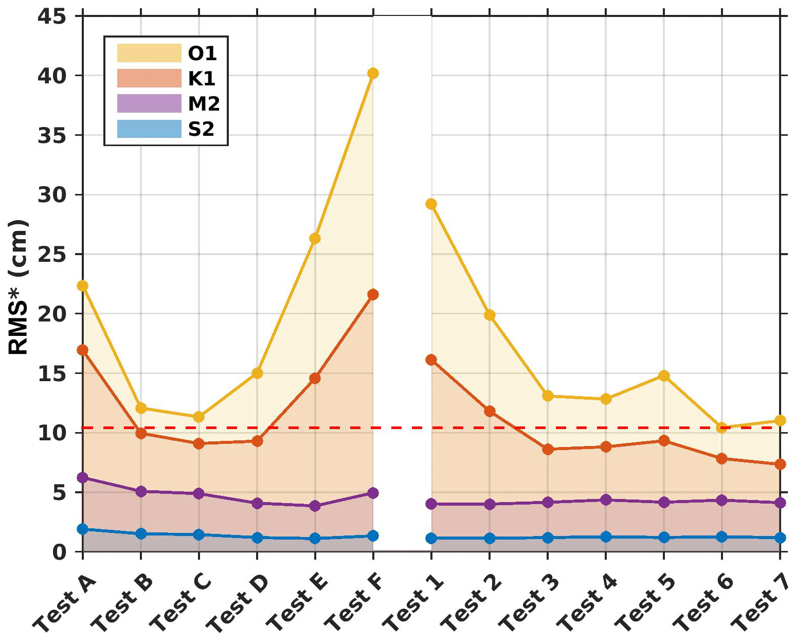
Figure 13Model complex errors (Appendix; Eq. A2) relative to altimetry data for tests listed in Table 1 performed with nonuniform values of z0 (SET3 and SET4). The space in between two lines corresponds to the errors for each wave. The yellow line corresponds to the cumulative errors for all four waves. The dashed red line corresponds to the smallest cumulative error, found for Test 6 (SET4), equal to 10.43 cm.
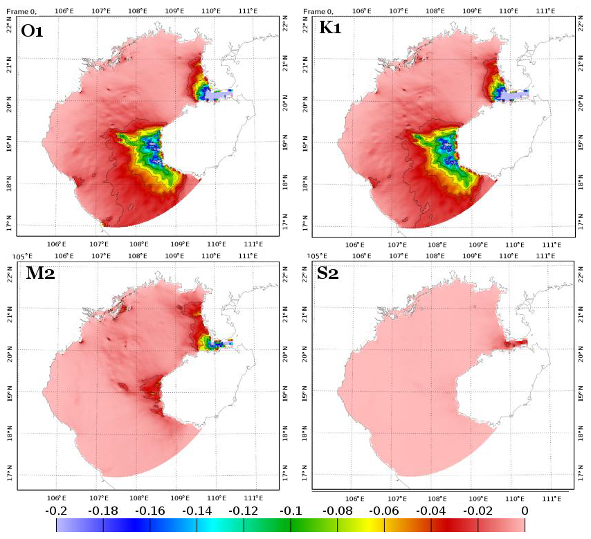
Figure 14Bottom dissipation flux (in watts per square meter) for O1, K1, M2, and S2 computed from model outputs of simulation Test 6.
Tests from SET3 suggest that the model sensitivity to bottom friction parameterization in the area of fine mud is limited and therefore poorly influences the cumulative errors over the GoT. This is due to the fact that tidal energy fluxes and bottom dissipation rates are extremely small in this area of fine mud near the Red River Delta, as can be seen in Fig. 14; most of the tidal dissipation occurs along the western coast of Hainan Island and in the Hainan Strait (values up to −0.2 W m−2 in these areas for O1, K1, and M2). Note that the value of r (which is here set to m following the optimization of Le Bars et al., 2010, over the Amazon shelf) could be tested and could lead to an optimized value for the GoT. However, this would have presumably not significantly affected the final tidal solutions since the choice of a linear parameterization in the area of fine mud did not significantly modify the tidal solutions.
Sensitivity to a spatially varying roughness length (SET4 and SET5 vs. SET2)
Improvement in the tidal solutions is obtained from SET4, i.e., by varying spatially the values of the bottom roughness length (imposing a logarithmic speed profile). The cumulative error of all four waves (yellow line) reach a minimum value of 10.43 cm for Test 6 ( dashed red line), which reduced the error found in SET2 by 0.53 cm. This value is reached by imposing values of m in regions 1 and 2 (Fig. 12) and m in region 3. Moreover, results from Test 1 and Test 2 show that the solutions largely depend upon the roughness length imposed in region 1 (z0 values of to m). Again, as already mentioned in the previous section, the remaining bathymetry-induced errors in our solutions have probably damaged the precise identification of truly physical friction parameterization in this spatially varying roughness length experiment.
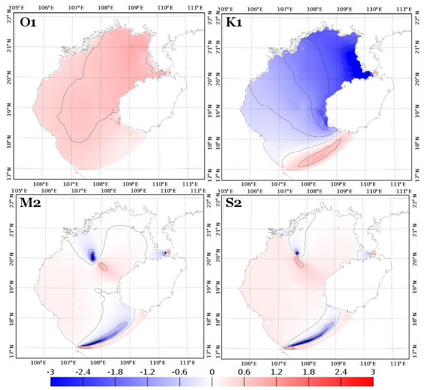
Figure 15Relative differences (in percent) between simulation Test 6 and simulation with ) compared to FES2014b-with-assimilation (as a reference) for the tidal harmonics of O1, K1, M2, and S2.
The significance of these results is assessed in Fig. 15. Simulation from Test 6 (SET4) better represents K1 harmonics, while simulation with varying m) (SET2) better represents O1 harmonics, taking FES2014b-with-assimilation as a reference. However the relative improvements from one simulation to another are again very small (< 3 %). Considering the semidiurnal waves, the differences are heterogeneous over the basin, with overall a slightly better representation (difference of ∼ 2 %) of the waves by the simulation with m) (SET2). These results finally suggest that differences between simulations from SET2 and SET3 are locally and globally insignificant and that the tidal solutions in the GoT are therefore not very sensitive to changes in bottom friction parameterization, from a constant z0 to a spatially varying z0.
Lastly, the results of the tests from SET5 did not show any improvement on the tidal solutions, compared to SET3 and SET4. The minimum cumulative error found in SET5 is reached by imposing z0 values that correspond exactly to the configuration of Test 6 in SET4 and is consequently also equal to 10.43 cm (i.e., the same as in SET4). This result again suggests that the model seems to be insensitive to high spatial refinement of the bottom sediment composition and associated roughness for the representation of tidal solutions.
3.2 Sensitivity to the bathymetry
Model bathymetry is a key parameter for tidal simulations. In order to evaluate the sensitivity of the model to the bathymetry, an additional sensitivity simulation is performed. First, the solutions obtained with the grid configuration with improved bathymetry and shoreline datasets described in Sect. 2.1 (Fig. 4) and a spatially varying roughness length (described in Test 6 from SET2, Table 1) with a logarithmic velocity profile are chosen as this choice of bottom roughness parameterization has shown the best tidal solutions (the least errors with respect to satellite altimetry) in Sect. 3.1.2. This simulation is named TKN hereafter. Second, we run a twin simulation with exactly the same configuration, parameterizations, and choice of parameters, except that the bathymetry and shoreline are not built from our improved dataset but from the default GEBCO bathymetry dataset and default-shoreline dataset. This simulation is hereafter named TKN-gebco. The results from these tests are presented in this section, where we evaluate the quality of the tidal solution obtained in our different simulations.
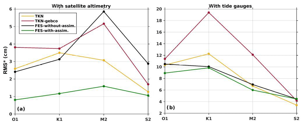
Figure 16RMS* errors (Appendix; Eq. A2) between numerical simulations (TKN, TKN-gebco, FES2014b-without-assimilation, and FES2014b-with-assimilation) and (a) altimetry data and (b) tide gauges for O1, K1, S2, and M2.
3.2.1 Average assessment over the domain
We first evaluate the tidal solution in average over the domain. Integrated along-track RMS* errors (Appendix; Eq. A2) between modeled and altimetry derived ocean tide harmonic constants (noted hereafter AH for altimetric harmonic) are shown in Fig. 16a. FES2014b-with-assimilation errors are globally always lower than errors given by the three other simulations, thanks to the assimilation of the satellite altimetry, i.e., 3 to 4.7 times lower for O1, 2.6 to 3.2 times lower for K1, 2.3 to 3.7 times lower M2, and 1.3 to 2.7 times lower for S2. As explained in Sect. 2.2.3, FES2014b-with-assimilation, which minimizes the error, is used in the following as a reference for the evaluation of our simulations to spatially complement altimetry data, which are only available along the altimetry tracks.
Along-track RMS* errors for M2 are reduced by 12 % in TKN-gebco relative to FES2014b-without-assimilation and by 47 % in TKN. The errors are also lower for S2, with a reduction in the errors by 41 % between FES2014b-without-assimilation and TKN-gebco and by 56 % between FES2014b-without-assimilation and TKN. On the other hand, both TKN and TKN-gebco simulations show bigger errors than FES2014b-without-assimilation for O1 and K1. However, the TKN simulation increases the errors for O1 by 7 % relative to FES2014b-without-assimilation, whereas TKN-gebco increases the errors by 58 %. The complex errors for K1 obtained from both TKN and TKN-gebco simulations increase by roughly 12 % and 20 % compared to FES2014b-without-assimilation, respectively. Such results illustrate the fact that K1 wavelengths are longer than the wavelengths of other waves considered here; e.g., at 60 m depth, K1 wavelength is 2000 km and M2 wavelength is 1000 km (Kowalik and Luick, 2013); therefore K1 is less sensitive to bathymetric variations. These results further illustrate FES model efficiency in tidal simulation in coastal areas, which is related in particular to the use of an unstructured triangle grid mesh specifically dedicated to finely adapt to complex coastal topography and coastline.
The mean absolute differences MAE (Appendix; Eq. A3) in amplitude and phase of the four tidal constituents between our simulation TKN and AH and between the two FES2014b products and AH are given in Table 2. The errors with respect to AH in both amplitude and phase is always reduced in TKN compared to FES2014b-without-assimilation (except for the phase of S2), from 1.2 times smaller for the phase of K1 to 2.7 times smaller for the amplitude of S2. However, errors with respect to AH are increased in both amplitude and phase in TKN compared to FES2014b-with-assimilation (except for the amplitude of S2).
Table 2Mean absolute differences (Appendix; Eq. A3) in amplitudes (in centimeters) and phase (in degrees) of M2, S2, O1, and K1 constituents between our reference TKN and satellite altimetry. For comparison, the two FES products compared with satellite altimetry, the work of Minh et al. (2014) compared with satellite altimetry, and the work Chen et al. (2009) compared to gauge stations are presented.

In addition, integrated RMS* errors between simulated and observed tidal harmonics from tide gauges are presented in Fig. 16b. Again, FES2014b-with-assimilation errors are globally always lower (for O1, K1 and M2) than errors given by the three other simulations, thanks to the assimilation of including those tide gauges data.
TKN-gebco increases the error for O1 by 27 % relative to FES2014b-with-assimilation, while TKN increases it by 16 %. TKN also slightly reduces (by 0.2 cm) the integrated tidal gauge RMS* errors for O1 compared to FES2014b-without-assimilation. The complex errors for K1 obtained from both TKN and TKN-gebco simulations increase by roughly 25 % and 90 % compared to FES2014b-with-assimilation, respectively. The errors for M2 are increased by 11 % with TKN and by 101 % with TKN-gebco compared to FES2014b-with-assimilation. Similar to the O1 case, TKN slightly reduces (by 0.3 cm) the RMS* errors for M2 compared to FES2014b-without-assimilation. Finally, both TKN and TKN-gebco simulations reduce the errors for S2 by 44 % and 9 % compared to FES2014b-with-assimilation, respectively. So for the four main tidal constituents, errors between simulated and observed tidal harmonics from tide gauges are significantly reduced in TKN compared to TKN-gebco.
These results show first that TKN configuration brings a clear improvement in tidal solutions compared to TKN-gebco configuration and second that it only slightly improves tidal solutions for some of the tidal components compared to FES2014b-without-assimilation. This last result is related to the use of an unstructured grid in FES2014b (with and without-assimilation), which is better adapted for the representation of the complex coastal topography than the structured grid that is used to optimize our TKN configuration since it will be used in our tridimensional structured grid model.
3.2.2 Spatial assessment of tidal solutions
The modeled O1, K1, M2, and S2 fields for TKN, TKN-gebco, FES2014b-without-assimilation, and FES2014b-with-assimilation are shown in Figs. 5–8. For each tidal component and simulation, the complex errors RMS* between these simulation results and AH are represented for each point of the altimetry track by the circles superimposed on the maps.
Both model simulations (TKN-gebco and TKN) reproduce well the distribution patterns of O1 harmonics compared to FES2014b-with-assimilation, improving the results compared to FES2014b-without-assimilation. Moreover, TKN solutions look more accurate than TKN-gebco. Errors with respect to AH for O1 (circles on the maps) are smaller than 10 cm in TKN-gebco and are reduced by 35 % compared to FES2014b-without-assimilation. They are further reduced in TKN; most of the errors are smaller than 5 cm and are reduced by 50 % compared to FES2014b-without-assimilation (Fig. 5). Note that higher errors of AH (of about 20 cm) are observed in TKN and TKN-gebco in the Hainan Strait and also near the coasts. These errors also appear in FES2014b-without-assimilation and, to a lesser extent (with values of about 15 cm in the Hainan Strait), in FES2014b-with-assimilation. The increase in complex errors in these particular areas could be explained by either model errors associated with errors in coastal bathymetry and shorelines, whose accuracy is decisive to shallow-water tidal waves, and/or erroneous altimetric data (land contamination in the altimeter footprint). For K1, even though both model simulations reproduce well the distribution pattern of the harmonics compared to FES2014b-with-assimilation, the errors with respect to AH compared to FES2014b-without-assimilation are not reduced in TKN-gebco nor or TKN (Fig. 6). Errors with respect to AH for K1 are equal to or smaller than 10 cm in FES2014b-without-assimilation, TKN-gebco, and TKN along the altimetry tracks and are extremely similar between those simulations. As observed for O1, larger and similar errors of about 20 cm are also observed in the Hainan Strait in TKN-gebco and TKN and in the two FES2014b products (though with smaller values of about 15 cm in FES2014b-with-assimilation, which includes assimilations). Furthermore, the angle of the radius of each circle indicates whether the error in amplitude or the error in phase dominates the complex error. The smaller the angle to the ordinate axis is, the more the error in phase dominates the complex error. On the contrary, the bigger the angle to the ordinate axis is, the more the error in amplitude dominates the complex error. When the angle to the ordinate axis approaches 45∘, the error in phase and the error in amplitude account equally for the complex error. For both O1 and K1, errors in phase are dominating the northern and central parts of the region, while the phase and amplitude account equally for the complex errors in the southernmost part of the region and in the Hainan Strait (Figs. 4c, d and 5c, d).
Figure 7 shows that M2 amplitude is globally overestimated by TKN and TKN-gebco compared to FES2014b-with-assimilation and FES2014b-without-assimilation, especially in the areas where the wave resonates (i.e., in the northeastern bay and in the southwestern part). Differences in FES2014b-without-assimilation are up to 30 to 35 cm in TKN and in TKN-gebco (in the northeastern bay), with amplitudes increasing by almost 45 % in model simulations. Both model simulations increase the resonance of M2 in the bays. These amplitude overestimations could be partially explained by the bathymetry dataset (TONKIN_bathymetry), which integrates nautical charts that underestimate depths, especially in shallow areas, for navigation purposes.
However, the amplitudes are underestimated near the amphidromic point (20.7∘ N, 107.3∘ E) by both simulations compared to FES2014b-without-assimilation (by up to 10 cm, roughly 80 %). Globally, errors with respect to altimetric harmonics are reduced in TKN by 30 % compared to TKN-gebco; most of the errors in TKN are smaller than 10 cm, while most of the errors in TKN-gebco are equal to or larger than 10 cm. Both simulations also show smaller errors with respect to AH south of Hainan Island compared to FES2014b-without-assimilation by up to 50 %, with errors of about 1 cm in FES2014b-without-assimilation and of about 0.5 cm in model simulations). Again, large errors are observed in the Hainan Strait in simulations and both FES2014b products; however the errors are reduced by 25 % in TKN and TKN-gebco compared to FES2014b-without-assimilation. Furthermore, these errors are dominated by errors in phase rather than in amplitude.
Lastly, both TKN and TKN-gebco model simulations overestimate the amplitude of S2 compared to FES2014b-with-assimilation and FES2014b-without-assimilation by up to 10 cm (approximately 50 %) in the southwestern and northeastern bays, where S2 resonates (Fig. 8). The resonance of S2 in the bays is therefore amplified in both model simulations. These amplitude amplifications observed in both models could be again partly explained by the bathymetric soundings of TONKIN_bathymetry that underestimate depths in shallow-water areas. Similar to the M2 case, both simulations also underestimate by roughly 5 cm the amplitude of S2 near the amphidromic point (20.7∘ N, 107.3∘ E) compared to the two FES2014b products. However, the complex errors with respect to AH are globally 50 % smaller in TKN (between 2 and 3 cm) than in TKN-gebco (between 4 and 5 cm). Furthermore, errors with respect to AH remain large in the Hainan Strait (up to 6 cm) in both FES products and both model simulations. In the very near coastal areas, errors with respect to AH in TKN and TKN-gebco are larger than in the rest of the basin (up to 6 cm). However, the errors with respect to AH in TKN are reduced by 30 % in the southwestern most part of the region. Like the M2 case, the complex errors of S2 are dominated all over the basin the by errors in phase rather than errors in amplitude.
3.3 Assessment of tidal solutions with previous studies
The mean absolute differences MAE (Appendix; Eq. A3) in amplitude and phase of the four tidal constituents between our simulation TKN and the satellite altimetry are given in Table 2. Our results are compared with the errors given in Minh et al. (2014) and in Chen et al. (2009). Minh et al. (2014) authors used a ROMS_AGRIF simulation at a resolution of over the GoT and compared their solutions to the same altimetric dataset as the one used in our study. Chen et al. (2009) compared their simulations, performed with ECOM (Extended Control Model) at a 1.8×1.8 km resolution (covering the area 16–23∘ N, 105.7–114∘ E), to gauge stations located along the GoT coast. Our simulation TKN shows large improvements in both amplitude and phase for the four constituents (except for the phase of M2) compared to the results of Minh et al. (2014). The errors are reduced by approximately 60 % for the amplitudes of M2 and S2 and by roughly 40 % for the amplitudes of K1 and O1. The errors in phase for O1 and K1 are also reduced by approximately 50 % in our simulation. Our results also show improvements compared with the errors proposed by Chen et al. (2009), for both amplitude and phase of S2 (by 65 % in amplitude and by 35 % in phase), O1 (by 50 % in amplitude and almost 60 % in phase), and K1 (by 68 % in amplitude and by 41 % in phase). Only the solutions of M2 are not improved by our simulation compared to Chen et al. (2009); they remain the same in amplitude and increase by 14 % in phase.
The improvement on our tidal solution from TKN compared to these two previous studies could be due first to the use of T-UGOm, which is specifically developed for purpose of tidal modeling, compared to models used by Minh et al. (2014) and Chen et al. (2009), which are hydrodynamical models not specifically conceived for tidal representation. Second, it could be due to our model configuration, which has been specifically optimized for tidal modeling purpose, in terms of grid resolution, bathymetry accuracy and resolution and bottom friction parameterization.
This study takes place in the framework of a more comprehensive modeling project, which aims at representing the transport and fate of the sediments from the Red River to the GoT. In this future study, the ocean dynamics and the sediment transport will be represented using the regional circulation model SYMPHONIE coupled with the sediment model MUSTANG. As tides have a major effect on the sediment dynamics within the estuaries and in the plume area (Pritchard, 1954, 1956; Allen et al., 1980; Fontes et al., 2008; Vinh et al., 2018), it is necessary to accurately represent the tidal processes before investigating the fine-scale sediment physics. This coupled model will allow for example the impact on tides of freshwater discharges and their strong seasonal variability to be studied, since this effect could be relatively important in the very nearshore coastal area.
The optimization of the configuration and parameterizations of this coupled tridimensional structured grid model is the final objective of this study. Optimizing the bathymetry and the parameterization of the bottom shear stress is crucial in shallow-water regional and coastal modeling since they both are critical parameters influencing the propagation and distortion of the tides (Fontes et al., 2008; Le Bars et al., 2010). The T-UGOm hydrodynamical model is used in this study in its spectral mode, which allows the user to perform fast and low-cost tests (compared to simulations with sequential models like SYMPHONIE) on various configurations. This strategy allows the assessment and quantification of the importance of each element considered and to determine the best configuration that will be applied in the above-mentioned forthcoming modeling study with SYMPHONIE–MUSTANG model.
In this study, we have first constructed an improved bathymetric dataset for the region of the GoT from digitalized nautical charts, soundings, intertidal DEM, and GEBCO bathymetry dataset. We also integrated into this bathymetry a new coastline dataset created with POCViP and satellite images, since the existing descriptions of the GoT coastlines, the Ha Long Bay islets and the Red River Delta were very poor. We then performed tests with the fast-solver 2D T-UGOm model on an unstructured grid refined in the Red River Delta and Ha Long Bay area to test the added value of this improved bathymetric dataset. With this new bathymetry, we have been able to reduce the errors (taking along-track altimetry data and tide gauges data as a reference) in the representation of M2 and S2 in T-UGOm simulations by 40 % and 25 %, respectively, and for O1 and K1 by 32 % and 6 %, respectively, compared to simulations that use the regular GEBCO dataset. Our improved bathymetry showed also better solutions for the semidiurnal waves than the tidal atlas FES2014b_hydrodynamics (errors reduced by 47 % for M2 and by 25 % for S2), even though our model seems to amplify their resonance. Moreover, our simulations also improved accuracy over the existing state of the art, by reducing the errors in amplitude of the semidiurnal waves by 60 %, the errors in amplitude of the diurnal waves by 40 %, and the errors in phase of the diurnal waves by 50 % compared to the results found by Minh et al. (2014). We believe the remaining errors in our best tidal solutions are due to potential lacks of details and resolution in the bathymetry. Since bathymetry directly impacts the speeds of the waves, bathymetric uncertainties may lead to alterations of the bottom shear stress.
The other key parameter influencing shallow-water tidal modeling is the bottom friction. In this study, the use of a constant CD parametrization or the use of a CD depending on the roughness length led to fairly similar results, in line with the results found by Le Bars et al. (2010) in the Amazon estuary. Furthermore, our study shows that the model is very sensitive to the values imposed on CD and z0, especially for the diurnal waves with errors increasing for extreme CD and z0 values. The lowest cumulative errors of all four waves (of 11.50 and 10.96 cm) were found for a uniform CD of m (prescribing a constant velocity profile) and for a uniform z0 of m (prescribing a logarithmic velocity profile), respectively. More importantly, the regionalization of the roughness length into three regions, for addressing the issue of representing the complexity of seabed composition and morphology, only slightly improved the accuracy of our simulation, with a lowest cumulative error for all four waves of 10.43 cm. Finer local adjustments of the roughness length or the choice of a linear velocity profile in the area of fine mud, did not significantly improve the accuracy of our simulations. In particular, the model in this configuration showed a very limited sensitivity to the presence of fine mud and a greater sensitivity to the roughness length values prescribed in the rest of the region, which was unexpected following the results of Le Bars et al. (2010) and explained by the low energy dissipation occurring in this area of fine mud.
Our results therefore quantitatively showed that the key parameter for the representation of tidal solutions over a shallow area like the GoT is the choice of bathymetry and shoreline dataset. Second, they revealed that the choice of the bottom stress parameterization does not significantly affect the performance of the model but that, for a given parameterization, the choice of the value of the friction coefficient is important. Furthermore, the use of T-UGOm in a 2D barotropic mode showed its efficiency in tidal spectral modeling with reduced simulation durations in both CPU and running times compared to structured grid numerical models. This allowed us to optimize our configuration in terms of grid, bathymetry, and bottom friction parameterization regarding the representation of the tidal solutions. Our resulting configuration brought a clear improvement in the tidal solutions compared to previous 3D simulations from the literature. The modeling strategy proposed here thus showed its efficiency in quickly optimizing the configuration that will be used in future works to address the issue of sediment transport and fate in the GoT, which was our primary objective. Finally, our configuration did not produce a clear improvement compared to FES2014b-without-assimilation and performed worse than FES2014b-with-assimilation, due to the use in both FES2014b simulations of an unstructured grid better representing the coastal topography complexity and the use of assimilation in FES2014b-with-assimilation. This underlines the importance of data assimilation for the production of tidal atlases and the need to go on developing satellite mission and in situ campaigns, despite the great improvements in numerical models in the last decades.
The evaluation of T-UGOm performances should be completed with the study of tidal currents, which is for now limited in the area due to in situ data unavailability but will be possible in the future thanks to the ongoing development of observed current datasets from high-frequency radars (Rogowski et al., 2019). Note also that the use of nautical charts for bathymetry construction could have led to overestimation of the tidal amplitudes in coastal areas, due to underestimation of real depths for navigation safety purposes. Furthermore, using bathymetry data available from digitalized navigation charts was a relatively simple way (compared to performing additional in situ measurements) to significantly improve the representation of topography in the coastal and estuarine areas of the GoT and could be applied successfully in other regions. However, updates and improvements in shoreline and bathymetry databases, particularly in the river channels, coastal areas, and in the Hainan Strait, would still improve the present results and especially reduce the tendency to increase errors at the coasts. Continuous efforts should be made in bathymetric data acquisition, and sharing them with the community should be a crucial concern.
For comparison of the simulations with the tidal harmonics from satellite altimetry, we first introduce the vectorial difference z, the complex difference, as
with the vector representing a given modeled tidal constituents (of amplitude Am and phase Gm) and zo the vector representing the observed tidal constituent.
For assessing the errors between the simulations (modeled constituents) and the altimetry (observed constituents), we compute the root-mean-square error (RMS*), like in Stammer et al. (2014) and in Minh et al. (2014). RMS* depends upon the vectorial difference z and is computed for each given constituent of each simulation as follows:
with Am and Gm being, respectively, the amplitude and phase of the modeled constituent, Ao and Go being the amplitude and phase of the constituent from satellite altimetry, and N being the number of points of comparison (i.e., the number of equivalent gauge stations along the altimetry tracks).
The model performance is also estimated using the mean absolute error (MAE). MAE measures the mean of the difference between the simulated and the observed values and is computed for each constituent according to
with Ei representing for each point i of the track the difference between the modeled constituent and the observed constituent. The MAE is separately calculated for amplitudes and for phases.
The model grid, which integrates the bathymetry and the coastline datasets developed in this study, is available in Zenodo/Piton (2019a). The T-UGOm model code installation instructions are updated at ftp://ftp.legos.obs-mip.fr/pub/ecola/README.html (last access: 21 December 2018), and the code and the updated tools and the poc-solvers are available on https://hg.legos.obs-mip.fr/tools/ (last access: 21 December 2018). An archive of the exact version of T-UGOm used in this study (version 2616:78a276dd7882) is also available in Zenodo/Piton (2019b). The configuration files (initial conditions and modified drag coefficients) are available in Zenodo/Piton (2019c). Model boundary conditions (i.e., FES2014b products) are available through: https://www.aviso.altimetry.fr/en/data/products/auxiliary-products/global-tide-fes.html (last access: 20 December 2018). The satellite altimetry track dataset of CTOH-LEGOS for model outputs comparison are available through: http://ctoh.legos.obs-mip.fr/products/coastal-products/coastal-products-1/sla-1hz (https://doi.org/10.6096/CTOH_X-TRACK_Tidal_2018_01, last access: 10 December 2018, Birol et al., 2017).
VP, MH, SO, and FL designed the experiments and VP carried them out. FL developed the model code and VP performed the simulations. VP, TH, and DA constructed the bathymetry dataset. VP prepared the article with contributions of MH, FL, SO, and PM.
The authors declare that they have no conflict of interest.
Map data copyrighted OpenStreetMap contributors and available from https://www.openstreetmap.org (last access: 20 May 2018). We thank the CTOH team of LEGOS (Toulouse) for providing coastal altimetry data. This paper is a contribution to the LOTUS International Joint Laboratory (http://lotus.usth.edu.vn/, last access: 5 January 2019).
This paper was edited by David Ham and reviewed by two anonymous referees.
Allen, G. P., Salomon, J. C., Bassoullet, P., Penhoat, Y. D., and Grandpré C.: Effects of tides on mixing and suspended sediment transport in macrotidal estuaries Sediment, Geology, 26, 69–90, 1980.
Amante, C. and Eakins, B. W.: ETOPO1 1 Arc-Minute Global Relief Model: Procedures, Data Sources and Analysis, NOAA Technical Memorandum NESDIS NGDC-24, National Geophysical Data Center, NOAA, https://doi.org/10.7289/V5C8276M, 2009.
Bentsen, M., Evensen, G., Drange, H., and Jenkins, A. D.: Coordinate Transformation on a Sphere Using Conformal Mapping, Mon. Weather Rev., 127, 2733–2740, 1999.
Birol, F., Fuller, N., Cancet, M., Nino, F., Delebecque, C., Fleury, S., Toublanc, F., Melet, A., Saraceno, M., and Léger, F.: Coastal applications from nadir altimetry: example of the X-TRACK regional products, Adv. Space Res., 59, 936–953, https://doi.org/10.1016/j.asr.2016.11.005, 2016.
Birol, F., Fuller, N., Lyard, F., Cancet, M., Niño, F., Delebecque, C., Fleury, S., Toublanc, F., Melet, A., Saraceno, M., and Léger, F.: Coastal Applications from Nadir Altimetry: Example of the X-TRACK Regional Products, Adv. Space Res., 59, 936–953, https://doi.org/10.1016/j.asr.2016.11.005, 2017.
Cai, S., Long, X., Liu, H., and Wang, S.: Tide model evaluation under different conditions, Cont. Shelf. Res., 26, 104–112, 2005.
Carrère, L. and Lyard, F.: Modeling the barotropic response of the global ocean to atmospheric wind and pressure forcing – comparison with observations, Geophys. Res. Lett., 30, 1–4, https://doi.org/10.1029/2002GL016473, 2003.
Carrère, L., Lyard, F., Cancert, M., Guillot, A., and Roblou, L.: FES2012: a new global tidal model taking advantage of nearly 20 years of altimetry, Proceedings of 20 years of Altimetry, Venice, 24–29 September, 2012.
Carrère, L., Lyard, F., Cancert, M., Guillot, A., and Picot, N.: FES2014, a new tidal model – Validation results and perspectives for improvements, presentation to ESA Living Planet Conference, Prague, 9–13 May, 2016.
Carter G. S. and Merrifield M. A.: Open boundary conditions for regional tidal simulations, Ocean Modell., 18, 194–209, https://doi.org/10.1016/j.ocemod.2007.04.003, 2007.
Chen, C., Li, P., Shi, M., Xuo, J., Chen, M., and Sun, H.: Numerical study of the tides and residual currents in the Leizhou Strait, Chin. J. Oceanol. Limnol., 27, 931–942, 2009.
Dang, T. H., Coynel, A., Orange, D., Blanc, G., Etcheber, H., and Le, L. A.: Long-term monitoring (1960–2008) of the river-sediment transport in the Red River Watershed (Vietnam): Temporal variability and dam-reservoir impact, Sci. Total Environ., 408, 4654–4664, https://doi.org/10.1016/j.scitotenv.2010.07.007, 2010.
Ding, Y., Chen, C., Beardsley, R. C., Bao, X., Shi, M., Zhang, Y., Lai, Z., Li, R., Lin, H., and Viet, N. T.: Observational and model studies of the circulation in the Gulf of Tonkin, South China Sea, J. Geophis. Res., 118, 6495–6510, https://doi.org/10.1002/2013JC009455, 2013.
Dronkers, J. J.: Tidal Computations in Rivers and Coastal Waters, North-Holland, Amsterdam, Inter-Sciences (Wiley), New-York, xii + 518 pp., 1964.
Eyre, B. and McConchie, D.: Implications of sedimentological studies for environmental pollution assessment and management: examples from fluvial systems in North Queensland and Western Australia, Sediment Geol., 85, 235–252, 1993.
Fang, G.: Tide and tidal current charts for the marginal seas adjacent to china, Chin. J. Oceanol. Limnol., 4, 1–16, 1986.
Fang, G., Kwok, Y. K., Yu, K., and Zhu, Y.: Numerical simulation of principal tidal constituents in the South China Sea, Gulf of Tonkin and Gulf of Thailand, Cont. Shelf Res., 19, 845–869, 1999.
Fontes, R. F. C., Castro, B. M., and Beardsley, R. C.: Numerical study of circulation on the inner Amazon Shelf, Ocean Dynam., 58, 187–198, 2008.
Gabioux, M., Vinzon, S. B., and Paiva, A. M.: Tidal propagation over fluid mud layers on the Amazon shelf, Cont. Shelf Res., 25, 113–125, 2005.
General Statistics Office: Statistical Yearbook of Vietnam 2017, Statistical Publishing House: Hanoi, Vietnam, available at: https://www.gso.gov.vn/default_en.aspx?tabid=515&idmid=5&ItemID=18941 (last access: 22 March 2020), 2017.
Gonzalez-Pola, C., Diaz del Rio, G., Ruiz-Villareal, M., Sanchez, R. F., and Mohn, C.: Circulation patterns at Le Danois bank, an elongated shelf-adjacent seamount in the Bay of Biscay, Deep-Sea Res. Pt. I, 60, 7–21, https://doi.org/10.1016/j.dsr.2011.10.001, 2012.
Guarnieri, A., Pinardi, N., Oddo, P., Bortoluzzi, G., and Ravaioli, M.: Impact of tides in a baroclinic circulation model of the Adriatic Sea, J. Geophys. Res., 118, 166–183, https://doi.org/10.1029/2012JC007921, 2013.
Herzfeld, M.: Improving stability of regional numerical ocean models, Ocean Dynam., 59, 21–46, https://doi.org/10.1007/s10236-008-0158-1, 2009.
Holt, J., Hyder, P., Ashworth, M., Harle, J., Hewitt, H. T., Liu, H., New, A. L., Pickles, S., Porter, A., Popova, E., Allen, J. I., Siddorn, J., and Wood, R.: Prospects for improving the representation of coastal and shelf seas in global ocean models, Geosci. Model Dev., 10, 499–523, https://doi.org/10.5194/gmd-10-499-2017, 2017.
Hu, J. Y., Kawamura, H., Hong, H. S., Kobashi, F., and Xie, Q.: Tidal features in the China Seas and their adjacent areas derives from TOPEX/Poseidon altimeter data, Chin. J. Oceanol. Limnol., 19, 293–305, 2001.
Kowalik, Z. and Luick, J.: The Oceanography of Tides, Fairbanks, USA. available at: https://www.uaf.edu/files/cfos/Kowalik/tide_book.pdf (last access: 20 March 2020), 2013.
Le, T. P. Q., Garnier, J., Billen, G., Théry, S., and Chau, V. M.: The changing flow regime and sediment load of the Red River, Viet Nam, J. Hydrol., 334, 199–214, 2007.
Le Bars, Y., Lyard, F., Jeandel, C., and Dardengo, L.: The AMANDES tidal model for the Amazon estuary and shelf, Ocean Model., 31, 132 1–49, https://doi.org/10.1016/j.ocemod.2009.11.001, 2010.
Lefebvre, J. P., Ouillon, S., Vinh, V. D., Arfi, R., Panché, J. Y., Mari, X., Thuoc, C. V., and Torréton, J. P.: Seasonal variability of cohesive sediment aggregation in the Bach Dang-Cam Estuary, Haiphong (Vietnam), Geo.-Mar. Lett., 32, 103–121, https://doi.org/10.1007/s00367-011-0273-8, 2012.
Le Hir, P., Cayocca, F., and Waeles, B.: Dynamics of sand and mud mixtures: A multiprocess-based modelling strategy, Cont. Shelf Res., 31, 135–149, https://doi.org/10.1016/j.csr.2010.12.009, 2011.
Lyard, F., Lefevre, F., Letellier, T., and Francis, O.: Modelling the global ocean tides: modern insights from FES2004, Ocean Dynam., 56, 394–415, https://doi.org/10.1007/s10236-006-0086-x, 2006.
Ma, F., Wang, Y., Li, Y., Ye, C., Xu, Z., and Zhang, F.: The application of geostatistics in grain size trend analysis: a case study of eastern Beibu Gulf, J. Geogr. Sci., 20, 77–90, 2010.
Madec, G. and Imbard, M.: A global ocean mesh to overcome the North Pole singularity, Clim. Dynam., 1, 381–388, 1996.
Manh, D. V. and Yanagi, T.: A study on residual flow in the Gulf of Tonkin, J. Oceanogr., 56, 59–68, 2000.
Maraldi, C., Chanut, J., Levier, B., Ayoub, N., De Mey, P., Reffray, G., Lyard, F., Cailleau, S., Drévillon, M., Fanjul, E. A., Sotillo, M. G., Marsaleix, P., and the Mercator Research and Development Team: NEMO on the shelf: assessment of the Iberia–Biscay–Ireland configuration, Ocean Sci., 9, 745–771, https://doi.org/10.5194/os-9-745-2013, 2013.
Marsaleix, P., Auclair, F., Floor, J. W., Herrmann, M. J., Estournel, C., Pairaud, I., and Ulses, C.: Energy conservation issues in sigma-coordinate free-surface ocean models, Ocean Model., 20, 61–89, https://doi.org/10.1016/j.ocemod.2007.07.005, 2008.
Milliman, J. D. and Meade, R. H.: World-wide delivery of river sediment to the oceans, J. Geol., 91, 1–21, 1983.
Monahan, D.: Mapping the floor of the entire world ocean: the general bathymetric chart of the ocean, J. Ocean. Tech., 3, 108 pp., 2008.
Natural Conditions and Environment of Vietnam Sea and Adjacent Area Atlas, Institute for Marine Geology and Geophysics, Hanoi (Vietnam), 118 pp., 2007.
Nguyen, N. T.: Some pecularities of the formation of tidal phenomena in the South China Sea, Okeanoloiia, 9, 235–249, 1969.
Nguyen, N. M., Marchesiello, P., Lyard, F., Ouillon, S., Cambon, G., Allain, D., and Dinh, V. U.: Tidal characteristics of the gulf of Tonkin, Cont. Shelf Res., 91, 37–56, https://doi.org/10.1016/j.csr.2014.08.003, 2014.
Nugroho, D., Koch-Larrouy, A., Gaspar, P., Lyard, F., Reffray, G., and Tranchant, B.: Modelling explicit tides in the Indonesian seas: An important process for surface sea water properties, Mar. Poll. Bull., 131, 7–18, https://doi.org/10.1016/j.marpolbul.2017.06.033, 2018.
Owens, P. N., Batalla, R. J., Collins, A. J., Gomez, B., Hicks, D. M., Horowitz, A. J., Kondolf, G. M., Marden, M, Page, M. J., Peacock, D. H., Petticrew, E. L., Salomons, W., and Trustrum, N. A.: Fine-grained sediment in river systems: environmental significance and management issues, River Res. Appl., 21, 693–717, 2005.
Pairaud, I. L., Lyard, F., Auclair, F., Letellier, T., and Marsaleix, P.: Dynamics of the semi-diurnal and quarter-diurnal internal tides in the Bay of Biscay – Part 1 : barotropic tides, Cont. Shelf. Res., 28, 1294–1315, https://doi.org/10.1016/j.csr.2008.03.004, 2008.
Pritchard, D. W.: A study of the salt balance in a coastal plain estuary, J. Mar. Res., 13, 133–144, 1954.
Pritchard, D. W.: The dynamic structure of a coastal plain estuary, J. Mar. Res., 15, 33–42, 1956.
Rogowski, P., Zavala-Garay, K., Shearman, K., Terrill, E., Wilkin, J., and Lam, T. H.: Air-sea-land forcing in the Gulf of Tonkin: Assessing seasonal variability using modern tools, Oceanogr., 32, 150–161, https://doi.org/10.5670/oceanog.2019.223, 2019.
Tong, S. S.: Mapping tidal flats in Vietnam using remote sensing techniques, PhD thesis, Univ. de Reims Champagne-Ardenne, 2016 (in French).
Smith, W. H. F. and Sandwell, D. T.: Global seafloor topography from satellite altimetry and ship depth soundings, Science, 277, 1957–1962, 1997.
Soulsby, R. L., Hamm, L., Klopman, G., Myrhaug, D., Simons, R. R., and Thomas, G. P.: Wave-current interaction within and outside the bottom boundary layer, Coastal Eng., 21, 41–69, 1993.
Stammer, D. Ray, R., Andersen, O., Arbic, B., Bosch, W., Carrère, L., Cheng, Y., Chinn, D., Dushaw, B., Egbert, G., Erofeeva, S., Fok, H., Green, J., Griffiths, S., King, M., Lapin, V., Lemoine, F., Luthcke, S., Lyard, F., Morison, J., Müller, M., Padman, L. Richman, J., Shriver, J., Shum, C., Taguchi, E., and Yi, Y.: Accuracy assessment of global barotropic ocean tide models, Rev. Geophys., 52, 243-282, https://doi.org/10.1002/2014RG000450, 2014.
Toublanc, F., Ayoub, N. K., Lyard, F., Marsaleix, P., and Allain, D. J.: Tidal downscalling from the open ocean to the coast: a new approach applied to the Bay of Biscay, Ocean Model., 124, 16–32, https://doi.org/10.1016/j.ocemod.2018.02.001, 2018.
van Maren, D. S. and Hoekstra, P.: Seasonal variation of hydrodynamics and sediment dynamics in a shallow subtropical estuary: the Ba Lat River, Vietnam, Estuar. Coast. Shelf Sci., 60, 529–540, 2004.
Vietnam maritime administration (Vinamarine): Approved planning for dredging in Hai Phong port, available at: http://vinamarine.gov.vn, last access: 15 July 2018.
Vignudelli, S., Cipollini, P., Roblou, L., Lyard, F., Gasparini, G. P., Manzella, G., and Astraldi, M.: Improved altimetry in coastal systems: Case study of the Corsica Channel (Mediterranean Sea), Geophys. Res. Lett., 32, 1–5, https://doi.org/10.1029/2005GL022602, 2005.
Vinh, V. D., Ouillon, S., Thanh, T. D., and Chu, L. V.: Impact of the Hoa Binh dam (Vietnam) on water and sediment budgets in the Red River basin and delta, Hydrol. Earth Syst. Sci., 18, 3987–4005, https://doi.org/10.5194/hess-18-3987-2014, 2014.
Vinh, V. D., Ouillon, S., and Dinh V. U.: Estuarine Turbidity Maxima and Variations of Aggregate Parameters in the Cam-Nam Trieu Estuary, North Vietnam, in Early Wet Season, Waters, 68, 1–33, https://doi.org/10.3390/w10010068, 2018.
Wang, X., Chao, Y., Zhang, H., Farrara, J., Li, Z., Jin, X., Park, K., Colas, F., McWilliams, J. C., Paternostro, C., Shum, C. K., Yi, Y., Schoch, C., and Olsson, P.: Modeling tides and their influence on the circulation in Prince Williams Sound, Alaska, Cont. Shelf Res., 63, S126–S137, https://doi.org/10.1016/j.csr.2012.08.016, 2013.
Wessel, P. and Smith, W. H. F.: A global, self-consistent, hierarchical, high-resolution shoreline database, J. Geophys. Res., 101, 8741–8743, https://doi.org/10.1029/96JB00104, 1996.
Wetzel, A., Szczygielski, A., Unverricht, D., and Stattegger, K.: Sedimentological and ichnological implacations of rapid Holocen flooding of a gently sloping mud-dominated incised valley – an example from the Red River (Gulf of Tonkin), Sedimentology, 64, 1173–1202, https://doi.org/10.1111/sed.12357, 2017.
Wyrtki, K.: Physical oceanography of the Southeast Asian waters, 195 pp., available at: https://escholarship.org/uc/item/49n9x3t4 (last access: 2 December 2018), 1961.
Ye, A. L. and Robinson, I. S.: Tidal dynamics in the South China Sea, Geophys. J. Roy. Astr. S., 72, 691–707, 1983.
Yu, M.: A preliminary study of tidal characteristics in the South China Sea, Acta. Oceanol. Sin., 6, 293–300, 1984.
Zenodo/Piton: Grid for T-UGO, https://doi.org/10.5281/zenodo.2640763, 2019a.
Zenodo/Piton: Version 2616:78a276dd7882 of T-UGOm code, https://doi.org/10.5281/zenodo.2669397, 2019b.
Zenodo/Piton: T-UGO configuration's files, https://doi.org/10.5281/zenodo.2640793, 2019c.