Description and evaluation of the UKCA stratosphere–troposphere chemistry scheme (StratTrop vn 1.0) implemented in UKESM1

Here we present a description of the UKCA StratTrop chemical mechanism, which is used in the UKESM1 Earth system model for CMIP6. The StratTrop chemical mechanism is a merger of previously well-evaluated tropospheric and stratospheric mechanisms, and we provide results from a series of bespoke integrations to assess the overall performance of the model.

We find that the StratTrop scheme performs well when compared to a wide array of observations. The analysis we present here focuses on key components of atmospheric composition, namely the performance of the model to simulate ozone in the stratosphere and troposphere and constituents that are important for ozone in these regions. We find that the results obtained for tropospheric ozone and its budget terms from the use of the StratTrop mechanism are sensitive to the host model; simulations with the same chemical mechanism run in an earlier version of the MetUM host model show a range of sensitivity to emissions that the current model does not fall within.

Whilst the general model performance is suitable for use in the UKESM1 CMIP6 integrations, we note some shortcomings in the scheme that future targeted studies will address.

1 Introduction

The ability to model the composition of the atmosphere is vital for a wide range of applications relevant to society at large. Atmospheric composition modelling can broadly be subdivided into two sub-disciplines: (1) aerosol processes and microphysics and (2) atmospheric chemistry. Coupling these processes in climate models is paramount for being able to simulate atmospheric composition at the global scale. The most societally important questions revolve around understanding how the composition of the atmosphere has changed over the past, attributing this change, understanding how this system is likely to change into the future, and what the impacts of these changes are on the Earth system and on human health. It is these pressing issues that have led to the development of the new UK Earth system model, UKESM1 (Sellar et al., 2019), which uses the UK Chemistry and Aerosol model (UKCA) (O'Connor et al., 2014; Morgenstern et al., 2009; Mulcahy et al., 2018) as its key component to simulate atmospheric composition in the Earth system. The key challenge UKCA is applied to is understanding and predicting how the concentrations of a range of trace gases, especially the greenhouse gases methane (CH₄), ozone (O₃) and nitrous oxide (N₂O), and aerosol species will evolve in the Earth system under a range of different forcings. UKCA simulates the processes that control the formation and destruction of these species. Here we describe and document the performance of the version of UKCA used in UKESM1, which includes a representation of combined stratospheric and tropospheric chemistry that enhances the capability of UKCA beyond the version used in the Atmospheric Chemistry and Climate Model Intercomparison Project (ACCMIP; Young et al., 2013; O'Connor et al., 2014) and the recent Chemistry–Climate Model Initiative (CCMI) intercomparison (Bednarz et al., 2018; Hardiman et al., 2017; Morgenstern et al., 2017). There have been a number of previous versions of UKCA with defined scopes, but we denote the version used in UKESM1 and described here as UKCA StratTrop to signify its purpose of the holistic treatment of composition processes in the troposphere and stratosphere.

As a result of the Chemistry–Climate Model Validation Activity (CCMVal), it was recommended that models which are aimed at simulating the coupled ozone–climate problem should include processes to enable interactive ozone in the troposphere and stratosphere (Morgenstern et al., 2010). Chemistry–climate models (CCMs) use schemes to describe the reactions that chemical compounds undergo. These chemistry schemes can be constructed to explicitly model a specific chemical reaction system (e.g. Aumont et al., 2005), but in most applications the chemistry schemes are heavily simplified. Until recently, models of atmospheric chemistry tended to focus on chemistry schemes formulated for limited regions of the atmosphere; detailed schemes have been constructed to examine phenomena such as stratospheric ozone depletion or tropospheric air pollution. Examples of this using the UKCA model framework are two studies of the effects of the eruption of Mt. Pinatubo, for which Telford et al. (2009) used the stratospheric scheme of Morgenstern et al. (2009) to study the effects of the eruption on stratospheric ozone, whereas Telford et al. (2010) used the tropospheric scheme of O'Connor et al. (2014) to examine the effects on tropospheric oxidising capacity. Whilst the chemical schemes described in O'Connor et al. (2014) (hereafter OC14) and Morgenstern et al. (2009) (hereafter MO09) have some overlap (for example the use of some common reactions) the schemes were developed with specific applications in scope. The reason for partitioning chemical complexity like this is to reduce the computational resources required. Moreover, simulations with these process limitations were found to be able to capture the phenomena of interest.

However, increases in computational power and a drive to answer a greater number of questions from model simulations have allowed models that simulate both the stratosphere and troposphere to be developed which are now widely used (e.g. Pitari et al., 2002; Jöckel et al., 2006; Lamarque et al., 2008; Morgenstern et al., 2012). The removal of the need for prescribed upper boundary conditions (for the stratosphere) and a more comprehensive chemistry scheme make their increased cost worth bearing. In this work, we describe the implementation of a combined chemistry scheme suitable for simulating the stratosphere and the troposphere within the UKCA model as used in UKESM1 (Sellar et al., 2019). This scheme, UKCA StratTrop, builds on and combines the existing stratospheric (MO09) and tropospheric schemes (OC14). In various configurations of UKCA (under the names HadGEM3-ES, UMUKCA-UCAM, NIWA-UKCA, ACCESS), this combined chemical scheme has already been used to study stratospheric ozone and its sensitivity to changes in bromine (Yang et al., 2014), subsequent circulation changes (Braesicke et al., 2013) and how it may be impacted by certain forms of geoengineering (Tang et al., 2014); the role of ozone radiative feedback on temperature and humidity biases at the tropical tropopause layer (TTL) (Hardiman et al., 2015); the effects on tropospheric and stratospheric ozone changes under climate and emissions changes following the Representative Concentration Pathways (RCPs) (Banerjee et al., 2016; Dhomse et al., 2018); climate-induced changes in lightning (Banerjee et al., 2014); and changes in methane chemistry between the present day and the last interglacial (Quiquet et al., 2015). The scheme has been included in model simulations as part of the CCMI project (Eyring et al., 2013; Hardiman et al., 2017; Morgenstern et al., 2017; Dhomse et al., 2018) as well as all future Earth system modelling studies using the UKESM1 model (Sellar et al., 2019).

This paper is organised in the following sections: in Sect. 2, we present a thorough description of UKCA StratTrop, including the physical model and details of the chemistry scheme, followed by a detailed description of the emissions used and some notes on the historical development of the scheme. In Sect. 3, we describe two 15-year simulations we have performed with UKCA StratTrop in an atmosphere-only configuration of UKESM1. In Sect. 4, we use these simulations to review the performance of UKCA StratTrop, focusing on the model's ability to simulate key features of tropospheric and stratospheric chemistry as simulated by other models or observed using in situ and remote sensing measurements. Finally, in Sect. 5, we discuss the performance of the model and make some recommendations for further targeted studies.

2 Model description

In this section, we present a thorough description of UKCA StratTrop, from the host physical model to the detailed process representation of the StratTrop chemistry scheme.

2.1 Physical model

The physical model to which the UKCA StratTrop chemistry scheme has been coupled is the Global Atmosphere 7.1/Global Land 7.0 (GA7.1/GL7.0; Walters et al., 2019) configuration of the Hadley Centre Global Environment Model version 3 (HadGEM3; Hewitt et al., 2011).

The coupling between the UKCA StratTrop chemistry scheme and the GA7.1/GL7.0 configuration of HadGEM3 is based on the Met Office's Unified Model (MetUM; Brown et al., 2012). As a result, UKCA uses aspects of MetUM for the large-scale advection, convective transport and boundary layer mixing of its tracers. The large-scale advection makes use of the semi-implicit semi-Lagrangian formulation of the ENDGame dynamical core (Wood et al., 2014) to solve the non-hydrostatic, fully compressible deep-atmosphere equations of motion. These are discretised onto a regular latitude–longitude grid, with Arakawa C-grid staggering (Arakawa and Lamb, 1977). The discretisation in the vertical uses Charney–Phillips staggering (Charney and Phillips, 1953) with terrain-following hybrid height coordinates. Although GA7.1/GL7.0 can be run at a variety of resolutions, as detailed in Walters et al. (2019), the resolution here is N96L85 (${\mathrm{1.875}}^{\circ }\times {\mathrm{1.25}}^{\circ }$ longitude–latitude), i.e. approximately 135 km resolution in the horizontal and with 85 terrain-following levels spanning the altitude range from the surface to 85 km. Of the 85 model levels, 50 lie below 18 km and 35 levels are above 18 km (Walters et al., 2019). Mass conservation of UKCA tracers is achieved with the optimised conservative filter (OCF) scheme (Zerroukat and Allen, 2015); use of this scheme for virtual dry potential temperature resulted in reducing the warm bias at the TTL (Hardiman et al., 2015; Walters et al., 2019). This conservation scheme is also used for moist prognostics (e.g. water vapour mass mixing ratio and prognostic cloud fields). Although this makes the conservation scheme for moist prognostics consistent with the treatment of UKCA tracers and virtual dry potential temperature, Walters et al. (2019) found that it had little impact on moisture biases in the lower stratosphere.

The convective transport of UKCA tracers is treated within the MetUM convection scheme. It is essentially the mass flux scheme of Gregory and Rowntree (1990) but with updates for downdrafts (Gregory and Allen, 1991), convective momentum transport (Gregory et al., 1997) and convective available potential energy closure. The scheme involves diagnosis of possible convection from the boundary layer, followed by a call to shallow or deep convection on selected grid points based on the diagnosis from step one, and then a call to the mid-level convection scheme at all points. One key difference between the convective treatment of UKCA chemical and aerosol tracers is that convective scavenging of aerosols (simulated with GLOMAP-mode) is coupled with the convective transport following Kipling et al. (2013), whereas for chemical tracers, convective transport and scavenging are treated independently. Further details on the convection scheme in GA7.1 can be found in Walters et al. (2019). Finally, mixing over the full depth of the troposphere is carried out by the so-called “boundary layer” scheme in GA7.1; this scheme is that of Lock et al. (2000) but with updates from Lock (2001) and Brown et al. (2008).

The GA7.1/GL7.0 configuration described in Walters et al. (2019) already includes the two-moment GLOMAP-mode aerosol scheme from UKCA (Mann et al., 2010; Mulcahy et al., 2018, 2020), in which sulfate and secondary organic aerosol (SOA) formation is driven by prescribed oxidant fields. In the UKCA–StratTrop configuration described here, the oxidants driving secondary aerosol formation are fully interactive; this coupling between UKCA chemistry and GLOMAP-mode is fully described in Mulcahy et al. (2020). Together with dynamic vegetation and a terrestrial carbon and nitrogen scheme (Sellar et al., 2019), GA7.1/GL7.0 and UKCA StratTrop make up the atmospheric and land components of the UK Earth system model, UKESM1 (Sellar et al., 2019), which forms part of the UK contribution to the Sixth Coupled Model Intercomparison Project (CMIP6; Eyring et al., 2016).

2.2 Chemistry scheme

The UKCA StratTrop scheme is based on a merger between the stratospheric scheme of MO09 and the tropospheric “TropIsop” scheme of OC14. StratTrop simulates the O_x, HO_x and NO_x chemical cycles and the oxidation of carbon monoxide, ethane, propane, and isoprene in addition to chlorine and bromine chemistry, including heterogeneous processes on polar stratospheric clouds (PSCs) and liquid sulfate aerosols (SAs). The level of detail of the VOC oxidation is far from the complexity of explicit representations (e.g. Aumont et al., 2005), but the VOCs simulated are treated as discrete species.

Wet deposition is parameterised using the approach of Giannakopoulos et al. (1999). Dry deposition is parameterised employing a resistance type model (Wesely, 1989) using the implementation described in OC14, updated to account for advancements in the Joint UK Land Environment Simulator (JULES; Best et al., 2011), in particular a significant increase in land surface types (an increase from 9 to 27; see below for more details). Interactive photolysis is represented with the Fast-JX scheme (Neu et al., 2007), as implemented in Telford et al. (2013). Fast-JX covers the wavelength range of 177 to 750 nm. For shorter wavelengths, effective above 60 km of altitude, a correction is applied to the photolysis rates following the formulation of Lary and Pyle (1991).

The StratTrop scheme includes emissions of 12 chemical species: nitrogen oxide (NO), carbon monoxide (CO), formaldehyde (HCHO), ethane (C₂H₆), propane (C₃H₈), acetaldehyde (CH₃CHO), acetone ((CH₃)₂CO), methanol (CH₃OH) and isoprene (C₅H₈) in addition to trace-gas aerosol precursor emissions (dimethyl sulfide (DMS), sulfur dioxide (SO₂) and monoterpenes). For the implementation used in UKESM1, emissions may be prescribed or interactive and are described in more detail in Sect. 2.6.1 to 2.6.3. A further seven long-lived species (N₂O, CF₂Cl₂, CFCl₃, CH₃Br, COS, H₂ and CH₄) are constrained by lower boundary conditions; for more details see Sect. 2.6.4.

Table 1 List of chemical species in UKCA StratTrop. Species in italics are not advected tracers but are calculated using a steady-state approximation. Species in bold are set as constant mixing ratios throughout the atmosphere.

^*The molecular mass of Sec_Org is set to 150 g mol⁻¹.

UKCA StratTrop was developed by starting with the stratospheric chemistry scheme (MO09) and adding aspects of chemistry unique to the tropospheric scheme (OC14). In most cases the formulation and reaction coefficients are taken from reference evaluations (JPL and IUPAC) or the Master Chemical Mechanism, as detailed in OC14. Table 1 provides a list of the chemical tracers included in the StratTrop configuration used in UKESM1. In total the model employs 84 species and represents the chemistry of 81 of these. O₂, N₂ and CO₂ are not treated as chemically active species. Note that the scheme has a simplified treatment of stratospheric halocarbons and lumps all chlorine and bromine source gases into CFC-11, CFC-12 and CH₃Br. This chemistry scheme accounts for 199 bimolecular reactions (Table S1), 25 unimolecular and termolecular reactions (Table S2), 59 photolytic reactions (Table S3), 5 heterogeneous reactions (Table S4) and 3 aqueous-phase reactions for the sulfur cycle (Table S5). Hence, UKCA–StratTrop describes the oxidation of organic compounds – e.g. methane, ethane, propane and isoprene and their oxidation products – coupled to the inorganic chemistry of O_x, NO_x, HO_x, ClO_x and BrO_x using a continuous set of equations with no artificial boundaries imposed on where to stop performing chemistry. Except for water vapour, at the top two levels, the mixing ratios of all species are held identical to those at the third-highest level. The time-dependent chemical reactions are integrated forward in time using an implicit backward Euler solver with Newton–Raphson iteration (Wild and Prather, 2000). This solver has a relative convergence criterion of 10⁻⁴ with a time step of 60 min throughout the atmosphere. An extensive discussion of the solver used here is presented in Esentürk et al. (2018).

The treatment of polar stratospheric cloud (PSC) has been recently expanded in UKCA (Dennison et al., 2019), but these improvements did not make it into the UKESM1 version of UKCA discussed here, which remains unmodified from the original Morgenstern et al. (2009) scheme. The abundance of nitric acid trihydrate (NAT) and mixed NAT–ice polar stratospheric clouds is calculated following Chipperfield (1999) assuming thermodynamic equilibrium with gas-phase HNO₃ and water vapour; the treatment of reactions on liquid sulfate aerosol also follows Chipperfield (1999). Sedimentation of PSCs is included in the model, whilst dehydration is handled as part of the model's hydrological cycle. Denitrification is prescribed in the same way as in Chipperfield (1999) with two different sedimentation velocities. We refer the reader to Morgenstern et al. (2009) and Dennison et al. (2019) for further details.

The stratospheric sulfate aerosol optical depth, used in the radiation scheme of MetUM, is modified to be consistent with the aerosols used in the heterogeneous chemistry which, by default, are taken from a surface area density climatology prepared for the CMIP6 model intercomparison (Beiping Luo, personal communication, 2016). The surface aerosol density is converted to a mass mixing ratio using a climatology of particle size (Thomason and Peter, 2006) and assuming a density of 1700 kg m⁻³.

2.3 Photolysis

The most significant new development relative to MO09 and OC14 in the UKCA–StratTrop scheme used in UKESM1 is the interactive Fast-JX photolysis scheme, which is applied to derive photolysis rates between 177 and 750 nm (Neu et al., 2007) as described in Telford et al. (2013). This is an important new addition as it enables interactive treatment of photolysis rates (key drivers for the photochemistry of the atmosphere) under changing climate and atmospheric composition. For shorter wavelengths relevant above 60 km, a correction is added to account for photolysis occurring between 112 and 177 nm, following Lary and Pyle (1991).

In older versions of UKCA (i.e. MO09 and OC14) precalculated photolysis frequencies were applied in the model. Sellar et al. (2019) show a comparison of these and we note here that the switch from precalculated to online interactive photolysis calculations has had a significant effect on shortening the model-simulated methane lifetime and increasing the tropospheric mean [OH] (Telford et al., 2013; O'Connor et al., 2014; Voulgarakis et al., 2009), as shown in Fig. 4.

2.4 Dry deposition

In UKCA the representation of dry deposition follows the resistance-in-series model as described by Wesely (1989) in which the removal of material at the surface is described by three resistances: r_a, r_b and r_c. The deposition velocity v_d (m s⁻¹) is then a function of these three resistance terms according to

$$\begin{array}{}\text{(1)}& v_{\text{d}}={\displaystyle \frac{\mathrm{1}}{r_a+r_b+r_c}},\end{array}$$

where r_a denotes the aerodynamic resistance to dry deposition, r_b is the quasi-laminar resistance term and r_c represents the resistance to uptake at the surface. Of these three terms r_c tends to be the most complex because it encompasses a variety of exchange fluxes, such as stomatal and cuticular uptake and assimilation by soil microbes. The uptake at the surface also depends strongly on the presence of dew, rain or snow, which can interrupt the deposition process altogether.

Surface dry deposition is calculated interactively at every time step for a number of atmospheric gas-phase species (see Table 1 for a list of deposited species). The aerodynamic resistance r_a is given by

$$\begin{array}{}\text{(2)}& r_a={\displaystyle \frac{\ln \left(\frac{z}{z_{\mathrm{0}}}\right)-\mathrm{\Psi }}{k\times u^{*}}},\end{array}$$

where z₀ is the roughness length, Ψ denotes the Businger dimensionless stability function, k is the von Karman constant and u^* is the friction velocity; r_a represents the resistance to turbulent mixing in the boundary layer and therefore depends crucially on the stability of the boundary layer. It is independent of the chemical species that is deposited.

The quasi-laminar resistance r_b, on the other hand, depends on the chemical and physical properties of the deposited species. It describes the transport through the thin, laminar layer of air closest to the surface. Transport through this layer is diffusive due to the absence of turbulent mixing.

The third resistance term r_c depends on both the physico-chemical properties of the deposited species and the properties and condition of the respective surface to which deposition occurs. The surface can be anything from bare soil or rock to vegetation and even urban environments. Surface uptake varies with season, time of day and current meteorological conditions. The largest individual surface type is water in the form of the world's oceans. In this latter case solubility clearly plays the key role (Hardacre et al., 2015; Luhar et al., 2017).

A particularly important surface uptake process is the deposition flux to the terrestrial vegetation. In this case a number of pathways exist which are commonly integrated into the so-called “big-leaf” model (Smith et al., 2000; Seinfeld and Pandis, 2006). Of all the deposition pathways manifesting in vegetated regions, for most species the most important is uptake through the stomata. Through these tiny pores in the leaf surface plants take up carbon dioxide from the atmosphere and exchange water vapour and oxygen with it. This exchange also includes all other species that make up the ambient air, including pollutants such as ozone. For this, the specific type of vegetation is crucial. Ozone deposition fluxes, for instance, vary widely between forests and grasslands.

The calculation of the surface resistance term and land surface type information provided by the dynamic vegetation model JULES (Best et al., 2011; Clark et al., 2011) is used in UKCA. JULES forms part of UKESM1 and is thus coupled with UKCA. Within JULES, various land surface type configurations may be selected. In the most simple configuration, which was also used in the UKESM1 predecessor model HadGEM2-ES, any land-based grid box at the surface can be subdivided into variable-sized fractions assigned to any of nine different surface types: broadleaf trees, needleleaf trees, C₃ grasses, C₄ grasses, shrubs, bare soil, rivers and lakes, urban environments, and ice. Non-land grid boxes are treated separately.

Since then, the number of land surface types in JULES has increased substantially (see Harper et al., 2018). Apart from the original 9-tile version (five vegetation and four non-vegetation types), 13-, 17- and also 27-tile configurations are now included. The upgrade to the 13-tile configuration increases the number of vegetation types by introducing three broadleaf plant functional types (PFTs), two needleleaf PFTS and two shrub PFTS; the number of grass-related PFTs as well as the number of non-vegetation types remains the same in this configuration. The 17-tile configuration further extends the number of PFTs by introducing four cropland types, two C₃-grass-related and two C₄-grass-related PFTs; again, the number of non-vegetation types remains the same. Finally, the 27-tile land surface configuration, corresponding to the UKESM1 release configurations and the configurations used for this paper, introduces a substantial number of additional land ice tiles. Each of these land surface and PFT tiles offers a specific resistance to dry deposition of atmospheric gas-phase species.

For dry deposition of aerosols a slightly different treatment is taken to that described above, and we direct the reader to Mulcahy et al. (2020) and references therein for more details.

2.5 Wet deposition

The wet deposition scheme employed in UKCA for the removal of tropospheric gas-phase species through convective and stratiform precipitation is the same as that described in O'Connor et al. (2014). The original scheme was implemented from the TOMCAT chemistry transport model (CTM) where it previously had been validated by Giannakopoulos (1998) and Giannakopoulos et al. (1999). In this paper we provide a brief description of the scheme but will not present an evaluation because there have been no changes since the last published version. For an in-depth performance evaluation in UKCA we refer to Sect. 3.4 in O'Connor et al. (2014).

Following a scheme originally developed by Walton et al. (1988) wet deposition is parameterised as a first-order loss process which is calculated as a function of the three-dimensional convective and stratiform precipitation. The climate model provides the required precipitation activity to UKCA. The wet scavenging rate r is calculated at every grid box and time step according to

$$\begin{array}{}\text{(3)}& r=S_j\times p_j\left(l\right),\end{array}$$

where S_j is the wet scavenging coefficient for precipitation type j (cm⁻¹) and p_j(l) is the precipitation rate for type j (convective or stratiform), provided at model level l (cm h⁻¹).

Scavenging coefficients for nitric acid (HNO₃) of 2.4 and 4.7 cm⁻¹ for stratiform and convective precipitation, respectively, are applied (see Penner et al., 1991). These parameters are scaled down for individual species using the fraction of each species in the aqueous phase, f_aq, calculated by

$$\begin{array}{}\text{(4)}& f_{\text{aq}}={\displaystyle \frac{L\times H_{\text{eff}}\times R\times T}{\mathrm{1}+L\times H_{\text{eff}}\times R\times T}},\end{array}$$

where L represents the liquid water content, R is the universal gas constant, T denotes ambient temperature and H_eff is the effective Henry's law constant for each species. H_eff includes the effects of solubility, dissociation and complex formation. Tables S6, S7 and S8 (in the Supplement) summarise the parameters used in the UKCA wet deposition scheme for each soluble species included in the StratTrop chemical mechanism.

Furthermore, in the scheme precipitation only occurs over a fraction of the grid box. This fraction is assumed to be 1.0 and 0.3 for stratiform and convective precipitation, respectively. These fractions are applied in the calculation of the grid-box mean wet scavenging rate for both precipitation types after which point the two rates are added together.

2.6 Emissions

This section describes the implementation of tropospheric ozone precursor emissions used in the UKCA StratTrop scheme in detail. The scheme includes the emissions of nine chemical species: nitric oxide (NO), carbon monoxide (CO), formaldehyde (HCHO), ethane (C₂H₆), propane (C₃H₈), acetaldehyde (MeCHO), acetone (Me₂CO), isoprene (C₅H₈) and methanol (MeOH). Emissions to UKCA can be broadly classified into two categories: offline, where pre-computed fluxes are read from input files, and online, where fluxes are computed in real time during the simulation by making use of online meteorological variables from the MetUM. The implementation of offline emissions will be described in Sect. 2.6.1. Examples of online emissions currently in UKCA StratTrop are biogenic volatile organic compound (BVOC) emissions (Sect. 2.6.2) and lightning NO_x (Sect. 2.6.3). All emissions, including offline emissions, have interannual variability over the time period of the model simulations.

When UKCA StratTrop is coupled to the UKCA aerosol scheme, GLOMAP-mode (Mann et al., 2010) as here, there are additional trace-gas aerosol precursor emissions for dimethyl sulfide (DMS), sulfur dioxide (SO₂) and monoterpenes (C₁₀H₁₆). These emissions will be discussed in the context of the UKESM1 aerosol performance in Mulcahy et al. (2020); the focus here will solely be on the tropospheric ozone precursor emissions. Table S10 and Figs. S7–S8 summarise the mean global annual emissions totals for the time period considered here (2005–2014) and their global and seasonal distributions.

2.6.1 Offline anthropogenic and natural emissions

Offline tropospheric ozone precursor emissions are either injected into the model's lowest layer or, in the case of aircraft emissions and some biomass burning emissions, injected into a number of model levels. The emissions are added to the appropriate UKCA tracers (see Table 1) and mixed simultaneously by the boundary layer mixing scheme (Sect. 2.1). While boreal and temperate forest and deforestation emissions (van Marle et al., 2017) of black carbon (BC) and organic carbon (OC) are considered “high level” (Mulcahy et al., 2020) and are spread uniformly up to level 20 (∼ 3 km in L85), all gas-phase biomass burning emissions are added to the surface layer.

For anthropogenic emissions, we make use of historical (1750–2014) annual emissions of reactive gases from the Community Emissions Data System (CEDS; Hoesly et al., 2018) that were prepared for use in CMIP6. The CEDS emissions are generally greater than those of other emission datasets (e.g. Lamarque et al., 2010) for the years that are used in the simulations evaluated here (i.e. 2005–2014). Biomass burning emissions are taken from van Marle et al. (2017). They combined satellite observations from 1997 with various proxies and output from six fire models participating in the Fire Model Intercomparison Project (FireMIP; Rabin et al., 2017) to provide a complete dataset of biomass burning emissions from 1750 to 2014 for use in CMIP6. As was the case for anthropogenic emissions, emissions from the years 2005–2014 are used here. For both anthropogenic and biomass burning, the emissions were re-gridded from their native resolution to N96L85 while conserving global annual totals and seasonal cycles. Emissions of all C₂ and C₃ VOCs are included as ethane and propane, respectively.

For natural emissions which are not simulated, offline emissions are prescribed through the provision of pre-computed fluxes. For example, oceanic emissions of CO, ethane (including ethene – C₂H₄) and propane (including propene – C₃H₆) are taken from the POET (Granier et al., 2005) inventory for the year 1990, which contains one annual cycle with 12 monthly fluxes. These fluxes are applied perpetually to all years of the time series. Biogenic emissions of acetaldehyde (MeCHO) make use of combined emissions of MeCHO and other aldehydes from the MACCity-MEGAN emissions inventory (Sindelarova et al., 2014); biogenic emissions of CO, HCHO, MeOH and propane (including C₃H₆) are also taken from this inventory. For biogenic acetone emissions, emissions of acetone and other ketones from the MACCity-MEGAN emissions inventory (Sindelarova et al., 2014) are combined. Based on the years 2001–2010, a monthly mean climatology is derived and applied to all years (see Sect. 3 for the implementation of the emission in the model). Finally, soil emissions of NO_x are distributed according to Yienger and Levy (1995) and scaled to give a global annual total of 12.0 Tg NO yr⁻¹, again perpetually applied to all years.

2.6.2 Biogenic VOC emissions

In the standard configuration of UKCA StratTrop in UKESM1, emissions of organic compounds from the natural environment (BVOC) are added to UKCA interactively (Sellar et al., 2019). Specifically, emissions of isoprene (C₅H₈) and (mono)terpenes are online, the latter represented by a lumped compound in UKCA with the formula C₁₀H₁₆ and a corresponding molecular weight of 136 g mol⁻¹, and calculated by the interactive biogenic VOC (iBVOC) emission model (Pacifico et al., 2011). Emission fluxes are passed to UKCA at every model time step.

Figure 1 Tropical distribution of the LIS-observed (Lightning Imaging Sensor) climatological annual mean lightning flash density over the period 1999–2013 (a) in comparison with the modelled annual mean climatology from the period 2005–2014 (b). The corresponding standard deviation of the observed and modelled climatologies are shown in panels (c) and (d), respectively.

In iBVOC the emissions of isoprene are coupled to the gross primary productivity of the terrestrial vegetation (Arneth et al., 2007; Pacifico et al., 2011). The biogenic emission of all other organic compounds included in the iBVOC model, i.e. (mono)terpenes, methanol and acetone, follows the original model described in Guenther et al. (1995). Note that the current configuration of UKCA used in UKESM1 does not make use of the interactive emissions of methanol or acetone; these are offline as discussed in Sect. 2.6.1. To the best of our knowledge, in the case of the non-isoprene biogenic VOCs there is no equivalent process-based formulation for an interactive BVOC emission model applicable to Earth system models (ESMs).

For present-day conditions total global annual emissions of isoprene amount to 495.9 (± 13.6) Tg C yr⁻¹. This number represents the 10-year average annual total emission strength and the uncertainty quantified by the standard deviation over the 10-year period between 2005 and 2014 taken from a historic run with UKESM1 (Sellar et al., 2019). This is in good agreement with estimates reported for other emission models (e.g. Arneth et al., 2008; Guenther et al., 2012; Messina et al., 2016; Müller et al., 2008; Sindelarova et al., 2014; Stavrakou et al., 2009; Young et al., 2009). For the global annual total (mono)terpene emissions, iBVOC calculates 115.1 (± 1.6) Tg C yr⁻¹ over the same period of model simulation. This model estimate is in reasonably good agreement with the literature (e.g. Folberth et al., 2006; Lathière et al., 2006; Arneth et al., 2007, 2011; Acosta Navarro et al., 2014; Sindelarova et al., 2014; Bauwens et al., 2016; Messina et al., 2016).

In the configuration of UKCA StratTrop used in UKESM1, isoprene is included in the gas-phase chemistry but does not contribute to the formation of secondary organic aerosol (SOA). Emissions of (mono)terpenes are oxidised using a fixed yield approach (e.g. Kelly et al., 2018) to form SOA in the GLOMAP-mode aerosol scheme – see Table S1 and Mulcahy et al. (2020) for a detailed description and evaluation.

2.6.3 Emissions of NO_x from lightning

The lightning NO_x emissions scheme in UKCA StratTrop is based on the cloud-top parameterisation proposed by Price and Rind (1992). Based on satellite data and storm measurements, the lightning flash density is parameterised as

$$\begin{array}{}\text{(5)}& {\displaystyle }& {\displaystyle }{F}_{\text{l}}=\mathrm{3.44}\times {\mathrm{10}}^{-\mathrm{5}}{H}^{\mathrm{4.9}},\text{(6)}& {\displaystyle }& {\displaystyle }{F}_{\text{o}}=\mathrm{6.2}\times {\mathrm{10}}^{-\mathrm{4}}{H}^{\mathrm{1.3}},\end{array}$$

where F is the flash density (flash min⁻¹), H is the cloud-top height (km), and the “l” and “o” subscripts are used to represent the land and ocean, respectively, and to distinguish between the updraft velocities experienced over the two surfaces. The scheme also differentiates between cloud-to-cloud and cloud-to-ground flashes based on the grid cell latitude (Price and Rind, 1993) and is resolution-independent by the implementation of a spatial calibration factor (Price and Rind, 1994). A minimum cloud depth of 5 km is required for NO_x emissions to be activated and is diagnosed on a time-step basis from the physical model's convection scheme. For NO_x production, the parameterisation assumes that the production efficiency per unit of energy discharged is 25 ×10¹⁶ molec NO J⁻¹, with the energy discharged from cloud-to-ground flashes (3.0 ×10⁹ J flash⁻¹) being approximately 3 times greater than that for cloud-to-cloud (0.9 ×10⁹ J flash⁻¹) flashes (Schumann and Huntrieser, 2007).

This implementation is identical to that implemented in HadGEM2-ES (Collins et al., 2011) by O'Connor et al. (2014) except that NO_x emissions are now distributed linearly in log(pressure) rather than linearly in pressure. Whereas global annual lightning emissions in HadGEM2-ES were inadvertently too low (O'Connor et al., 2014; Young et al., 2013), here the emissions have been scaled to give an average global annual emission rate of 5.93 and 5.98 Tg N yr⁻¹ over the period 2005 to 2014 in the free-running and nudged simulations, respectively. When compared with anthropogenic, biomass burning and natural emissions, lightning contributes approximately 10 % to the global annual NO_x emission rate, consistent with estimates from Schumann and Huntrieser (2007).

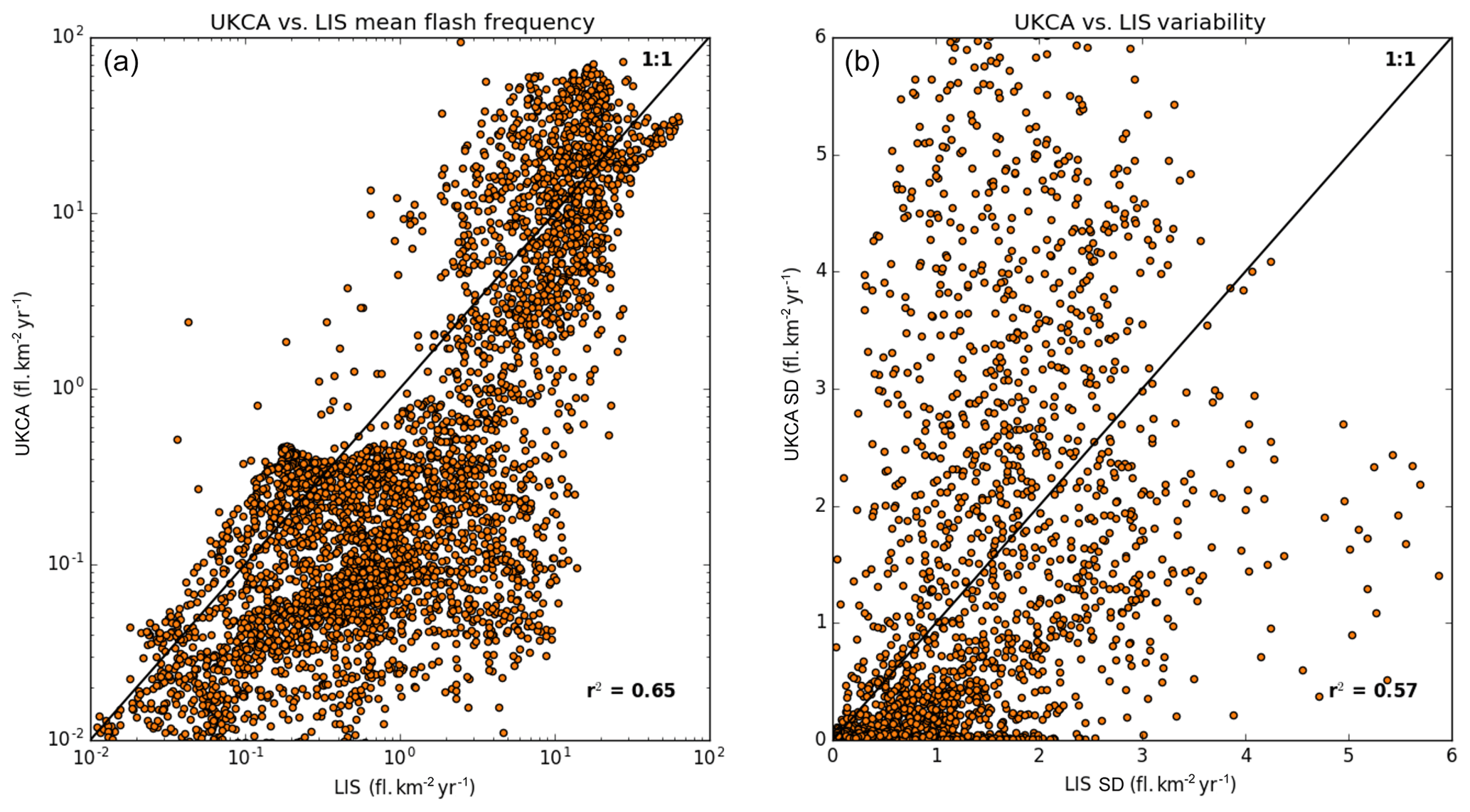
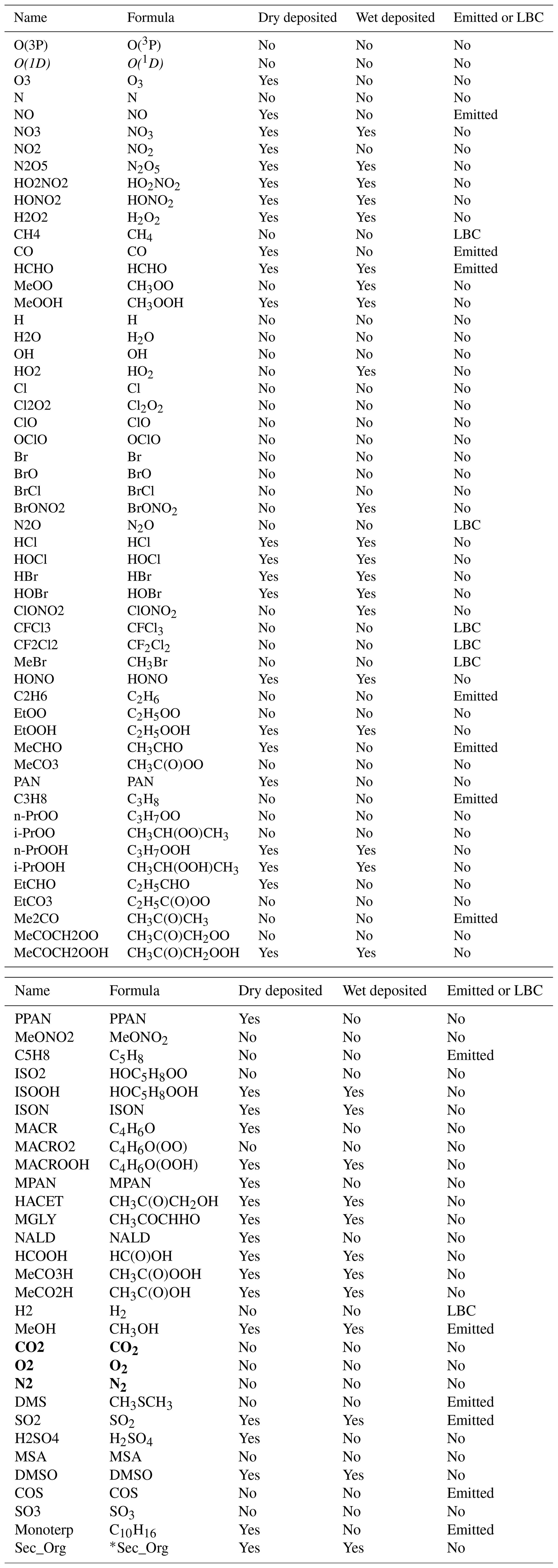
Figure 2 Scatter plot of the modelled versus the LIS-observed multi-annual mean lightning flash density (a) and the standard deviation (b).

Figure 1 shows tropical distributions of decadal mean annual flash density as observed by the Lightning Imaging Sensor (LIS) onboard the Tropical Rainfall Measuring Mission (TRMM) satellite (Theon, 1994) in comparison with the free-running simulation being evaluated here (see Sect. 3 for details). It demonstrates that UKCA is capable of capturing the broad features of the observed climatology, with peak densities over South America, Africa and East Asia; the spatial coefficient of determination (R²) between the modelled and observed climatology is 0.65 and 0.69 in the free-running and nudged (not shown) simulations, respectively. However, the model tends to be biased low in regions of low flash density (e.g. over the oceans and towards the extratropics) compared to the observations (Fig. 2), consistent with the assessment of Finney et al. (2014). In considering the variability, the spatial R² between the modelled and observed standard deviation is 0.57 and 0.59 in the free-running and nudged simulations, respectively. The variability from UKCA is comparable in magnitude to that observed over Africa, albeit displaced geographically. Over the Maritime Continent and South America, for example, UKCA overestimates the variability relative to the LIS observations.

Whilst the skill of the cloud-top parameterisation is good relative to other parameterisations (Finney et al., 2014), and the performance here in the free-running and nudged model simulations is consistent with that assessment, raising the diagnosed cloud-top height over land to the power of 4.9 makes the cloud-top parameterisation susceptible to model biases in cloud-top height, as noted by Allen and Pickering (2002) and Tost et al. (2007). Lightning is potentially a key chemistry–climate interaction in Earth system models, but the sensitivity to how it is represented (i.e. using cloud-top height (Banerjee et al., 2014) or ice-flux-based parameterisations; Finney et al., 2018) warrants further investigation. Indeed, Hakim et al. (2019) recently identified uncertainty in modelled lightning NO_x in the Indian subcontinent as being an important source of uncertainty in model simulations of tropospheric ozone in that region.

2.6.4 Lower boundary conditions

Lower boundary conditions are provided at the surface for the chemical species CH₄, N₂O, CFC-11 (CFCl₃), CFC-12 (CF₂Cl₂), CH₃Br, H₂ and COS. Values for H₂ and COS are fixed at 500 ppb and 482.8 ppt, respectively (invariant with time). Values for the remaining species are specified using time series data provided for the 5th Coupled Model Intercomparison Project (CMIP5) for the greenhouse gas concentrations (RCP Database, 2020). The values provided are valid on 1 July for each year specified and are linearly interpolated in time to give daily values if data for more than one time point are defined. CFC-11, CFC-12 and CH₃Br also contain contributions from other Cl- and Br-containing source gases which are not explicitly treated in the model to ensure that there is the correct stratospheric chlorine and bromine loading, with these contributing species given in Table 2. These values are converted into a two-dimensional “effective emission” field at each time step that is used to fix the surface concentrations of these species.

Table 2 List of halocarbons (not explicitly treated in the model) contributing to the lower boundary conditions of CFC-11, CFC-12 and CH₃Br. Note that H-1211 contributes to both CFC-11 and CH₃Br as it contains both Cl and Br. Contributions are included by moles of Cl or Br.

2.7 Coupling with other Earth system components

Secondary aerosol formation of sulfate and organic carbon in UKESM1 (Sellar et al., 2019) is determined by oxidants (OH, O₃, H₂O₂, NO₃) modelled interactively by the UKCA StratTrop chemistry scheme. For further details on the oxidation of sulfate and SOA precursors, chemistry–aerosol coupling, and the scientific performance of the aerosol scheme (GLOMAP-mode; Mann et al., 2010) in UKCA and UKESM1, the reader is referred to Mulcahy et al. (2020).

In the HadGEM2-ES model (Collins et al., 2011) used for CMIP5, radiative feedbacks between UKCA-modelled methane and tropospheric ozone concentrations were active (OC14); stratospheric ozone was prescribed and combined with the modelled interactive tropospheric concentrations. In UKESM1 (Sellar et al., 2019), however, the coupling between the UKCA-modelled radiatively active trace gases and the radiation scheme has been extended to include N₂O and stratospheric ozone (in addition to methane and tropospheric ozone). Although chlorofluorocarbons (CFCs) and hydrochlorofluorocarbons (HCFCs) are modelled in UKCA StratTrop, the radiation scheme cannot handle the speciation. Therefore, separate lumped species (CFC12-eq and HFC134a-eq) are prescribed in the radiation scheme (see Sect. 2.6.4 on how the lumping and mapping is done).

2.7.1 Heterogeneous chemistry couplings

In UKCA StratTrop as implemented in UKESM1, five different heterogeneous reactions are included (see Table S4). These reactions occur on the modelled soluble aerosol surface area, which in the troposphere is calculated interactively using GLOMAP-mode by summing over all soluble aerosol modes. In the stratosphere (defined here as being 12 km above the surface) the aerosol surface area comes from the stratospheric sulfate surface area density input climatology, discussed in Sellar et al. (2020). The combining of the stratospheric aerosol surface area density from the climatology and the interactive components of GLOMAP-mode is calculated at each UKCA time step, and only the soluble aerosol modes simulated by GLOMAP are included in the calculation.

Heterogeneous reactions are extremely important for simulating composition change in the stratosphere (Keeble et al., 2014), and there is increasing attention to the simulation of these processes in the troposphere (e.g. Jacob et al., 2000; Lowe et al., 2015). One of the most important tropospheric heterogeneous reactions is that of N₂O₅ on aerosol surfaces (Jacob et al., 2000). This reaction is complicated because of the dependence of the uptake parameter (γ) on the composition of the aerosol as well as on temperature and relative humidity (Bertram and Thornton, 2009). Macintyre and Evans (2010) suggest that models that use high values of γN₂O₅ (∼ 0.1) overestimate the impact of changing aerosol loadings on tropospheric composition through heterogeneous uptake. In UKCA StratTrop, γN₂O₅ is set at this higher value, 0.1, throughout the atmosphere. In part this compensates for the fact that there is an important missing aerosol surface in UKESM1 in the troposphere in the form of nitrate aerosol. The lack of nitrate aerosol is an issue for UKESM1 simulations of particulate matter, particularly in regions with high levels of ammonia emissions. An improved understanding of γN₂O₅ is needed to understand both the current composition and the combined impact of changing gas- and aerosol-phase composition. Whilst more sophisticated treatments of γN₂O₅ are available (e.g. Bertram and Thornton, 2009) and have been included in versions of UKCA, further work is required to improve this aspect of the mechanism for UKCA in UKESM1.

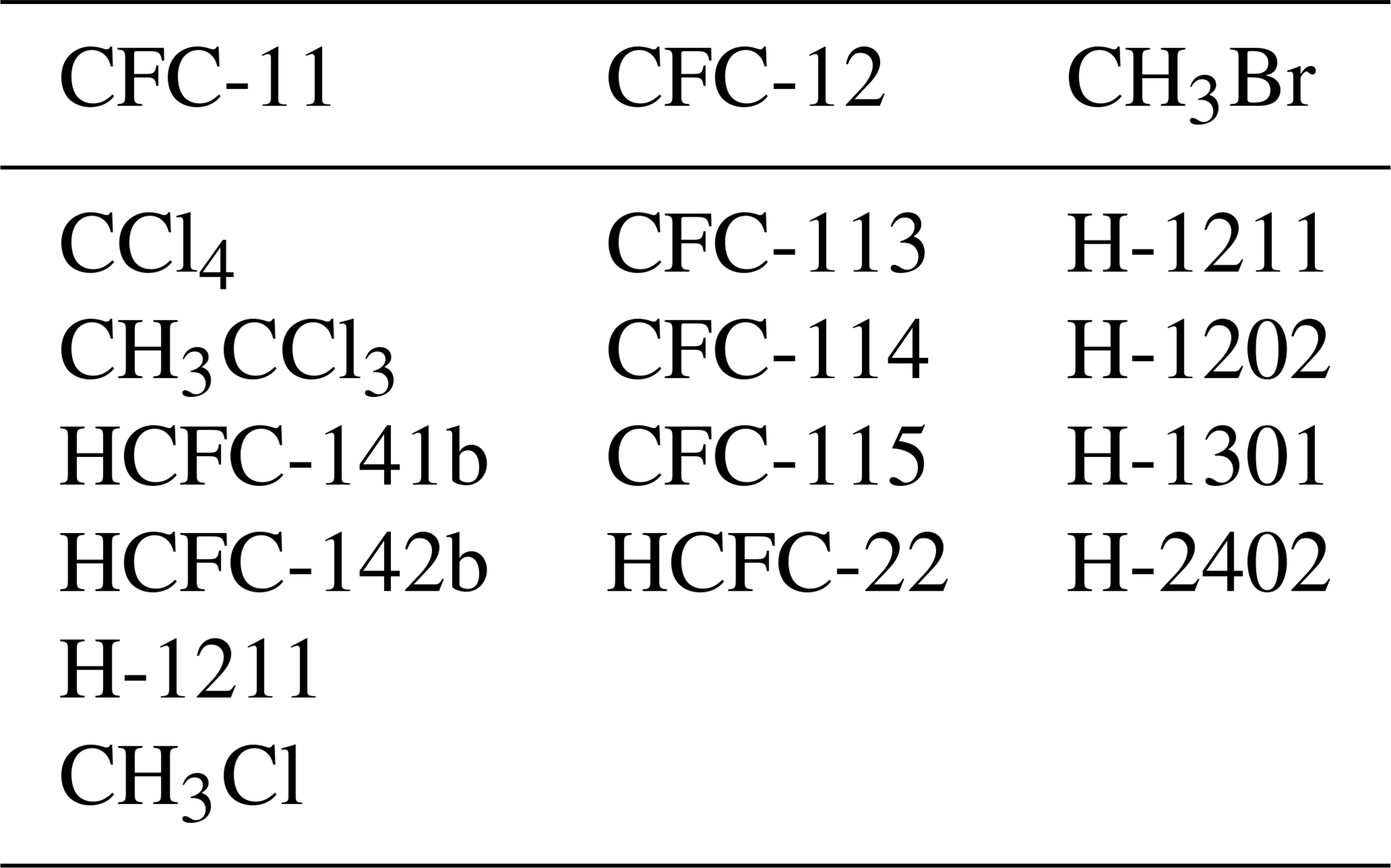
Figure 3 Multi-annual mean zonal-mean production of H₂O from the UKCA StratTrop mechanism in UKESM1. Panel (a) shows the production in moles per second and panel (b) in parts per billion per day, highlighting the larger relative source of water from chemical processes in the upper atmosphere.

2.7.2 Chemical production of H₂O

There are many chemical reactions which consume or produce water vapour in the troposphere and stratosphere. For example, reactions between the hydroxyl radical (OH) and VOCs usually result in the production of a water molecule.

$$\begin{array}{}\text{(7)}& \mathrm{OH}+\mathrm{VOC}\to {\mathrm{H}}_{\mathrm{2}}\mathrm{O}+\text{organic radical}\end{array}$$

In the troposphere the chemical source of water vapour is negligible compared with that from the oceans and evapotranspiration from the Earth's land surface, but given the low temperatures around the tropopause, chemically produced water is very important in the lower stratosphere. Furthermore, the main source of chemical water in the middle to upper stratosphere comes from the oxidation of CH₄. Complete oxidation of CH₄ to CO₂ can result in the net production of two water molecules.

In previous versions of UKCA, such as that used in HadGEM2-ES, the oxidation of CH₄ to produce chemical water was neglected. Instead, stratospheric water vapour was simulated using the following simple relationship:

$$\begin{array}{}\text{(8)}& \mathrm{2}\times \left[{\mathrm{CH}}_{\mathrm{4}}\right]+\left[{\mathrm{H}}_{\mathrm{2}}\mathrm{O}\right]=\mathrm{3.75}\left(\text{ppm}\right),\end{array}$$

where UKCA was used to calculate [CH₄]. In UKCA StratTrop as implemented in UKESM1 we now include interactive H₂O production from all chemical reactions in the mechanism. In this way UKCA now passes the water vapour field after the chemistry step back to the main climate model where it is used in other routines. The annual mean zonal-mean chemical production of H₂O as simulated by UKESM1 is shown in Fig. 3. There are two clear regions which dominate where H₂O chemical production takes place: in the tropical lower troposphere and the tropical upper stratosphere. In both regions the primary source of chemical water is the oxidation of CH₄. Figure 3 compares the absolute production of chemical water (panel a) and the production of chemical water as expressed in mixing ratio units (panel b). In this sense, panel (b) shows that the relative production of chemical water is greatest in the upper stratosphere. The contribution of this source of stratospheric H₂O to the present-day forcing of climate relative to the pre-industrial period will be assessed in O'Connor et al. (2019).

2.7.3 Future couplings

Although UKESM1 (Sellar et al., 2019) represents a significant enhancement in the representation of atmospheric chemistry and Earth system interactions, a number of key interactions are not included. For example, the coupling of aerosols with Fast-JX is omitted despite the impact of aerosols on the tropospheric photochemical production of ozone (e.g. Xing et al., 2017; Wang et al., 2019). This development is currently underway and will be included in future versions of UKCA and UKESM. Ozone damage to natural and managed ecosystems (e.g. Ashmore, 2005) has an important impact on the strength of carbon uptake by vegetation (Sitch et al., 2007; Oliver et al., 2018) and has yet to be implemented. In addition, although the terrestrial carbon cycle considers nitrogen availability and limitation, nitrogen deposition rates are prescribed in UKESM1; future work will include implementing a nitrate aerosol scheme in GLOMAP-mode and coupling the deposition of both oxidised and reduced nitrogen from the atmosphere to the terrestrial biosphere.

2.8 Historic development of the chemistry scheme

During the development of the StratTrop chemistry scheme, several simulations were run to test the scheme and its sensitivity to different (a) rate coefficients (updating the JPL and IUPAC recommendations), (b) reactions (by looking at the sensitivity to specific reactions associated with isoprene oxidation (Archibald et al., 2011) and the reaction between HO₂ and NO; Butkovskaya et al., 2005, 2007, 2009), (c) treatment of photolysis, (d) emissions and (e) deposition parameters. These one-at-a-time simulations are outlined in Table S9 in the Supplement. It should be noted that these simulations provide an ensemble of opportunity; they were not designed to probe model sensitivity in a targeted way. However, they result in some useful information which helped the development of the StratTrop mechanism. These simulations made use of an older version of the MetUM and an earlier atmosphere-only version of UKCA, which is now deprecated. That version of UKCA ran at a lower resolution than the version discussed in this paper and used in UKESM1 (about half the resolution). The results from these simulations are shown in Fig. 4 where they are compared against results from model intercomparison studies (further analysis of the model sensitivity tests is presented in Figs. S1–S6 in the Supplement). Figure 4 focuses on a subset of the full range of experiments performed but contextualises these by comparing to results from the ACCENT simulations discussed in Stevenson et al. (2006) (black dots) and the ACCMIP simulations discussed in Young et al. (2013) (orange dots). In addition to the early sensitivity tests (the blue dots in Fig. 4), we also show the results from the simulations presented here, labelled UKESM1 (red triangle in Fig. 4). The figure focuses on the relationship between methane lifetime and ozone chemical loss, important metrics for representing key sources and sinks of tropospheric OH (Wild, 2007). Both metrics are calculated by masking out the stratosphere. The methane lifetime is calculated by dividing the burden of methane in the model by the reaction flux between methane and OH in the troposphere, so it represents the lifetime with respect to OH in the troposphere. The ozone loss is calculated by summing the reaction fluxes which are key for O₃ loss in the troposphere (reactions of O₃ with HO_x species and the reaction between O(¹D) and H₂O). The experiments outlined in Table S9 and shown in Fig. 4 emphasise that the range in O₃ loss and CH₄ lifetime spanned by changing aspects of the UKCA model span a range as wide as that covered by the ACCMIP models (Young et al., 2013). In other words, the ensemble of opportunity from the early tests of the UKCA StratTrop scheme span as wide a range in the metrics presented as the structurally different ACCMIP and ACCENT models. Interestingly, the UKESM1 simulations discussed in this paper in detail lie close to the ACCENT ensemble (black dots), yet the early test simulations using the same chemical mechanism but an earlier version of the MetUM model do not (the blue cluster of dots). This highlights that structural changes in the underlying meteorological model can substantially influence key metrics of atmospheric composition through changes in the distribution of clouds, water vapour and other key variables.

Figure 4 Comparison of early tests of the StratTrop scheme running in an older version of UKCA (blue dots) with the scheme applied in UKESM1 (red triangle; free-running simulation), other CCMs which took part in the ACCMIP intercomparison (orange dots) and CTMs which took part in the ACCENT intercomparison (black dots). The letters in the legend (i.e. B–A) refer to the experiments outlined in Table S9.

These sensitivity studies highlight some important points. Simulations using kinetic data recommendations from IUPAC and JPL updated from 2005 to 2011 led to a decrease in model methane lifetime and an increase in ozone chemical loss flux (grey arrow), indicating increased photochemical activity. The attribution of which rate coefficients were dominant in this behaviour is outside the scope of this work. Similarly, we note that the metrics analysed are sensitive to lightning NO_x (Banerjee et al., 2014); decreasing the lightning NO_x emissions by 50 % (to ∼ 3 Tg yr⁻¹) results in an increased methane lifetime of ∼ 1 year (purple arrow). Figure 4 also highlights a non-linear response in the simulations to changes in isoprene emissions; scaling them by a factor of 2 (100 % increase and 50 % decrease; green arrows) leads to a highly non-linear response in the metrics analysed. Finally, we note that the change which had the biggest impact on the metrics was switching to the FAST-JX photolysis scheme (Telford et al., 2013) from precalculated photolysis rates and a lookup table (pink arrow). The main reason for this is that the precalculated photolysis rates had underestimated rates for the photolysis of O₃ to O(¹D). This behaviour has been documented previously (Voulgarakis et al., 2009; Telford et al., 2013).

In addition to the tests described above we found during the testing of the StratTrop scheme that inclusion of the termolecular reaction

$$\begin{array}{}\text{(9)}& {\mathrm{HO}}_{\mathrm{2}}+\mathrm{NO}+\mathrm{M}\to {\mathrm{HONO}}_{\mathrm{2}}+\mathrm{M},\end{array}$$

which has been shown to exhibit both pressure and water vapour dependence (Butkovskaya et al., 2005, 2007, 2009), led to large changes in the metrics analysed in Fig. 4 (see Sect. S1.2 of the Supplement for further details). Previous modelling work highlighted that this could have an important impact on the simulation of ozone (Cariolle et al., 2008). However, owing to uncertainty in its recommendation between the recent evaluations by JPL and IUPAC we have omitted it from the StratTrop scheme used in UKESM1.

3 Model simulations to evaluate UKCA StratTrop in UKESM1

In this section, we discuss a series of simulations that have been performed to evaluate the performance of the UKCA StratTrop scheme in UKESM1. These simulations link closely to the UKESM1 historical and AMIP simulations by using similar inputs, e.g. emissions, and crucially the version of UKCA StratTrop is identical to that used in UKESM1 (Sellar et al., 2019).

Simulations analysed in this paper have been carried out with an atmosphere-only configuration of UKESM1 (Sellar et al., 2019). The sea surface temperatures and sea ice cover used to drive the model are those specified for the historical period by the Sixth Coupled Model Intercomparison Project (CMIP6 project; Durack et al., 2016). Land cover fraction, vegetation canopy height and leaf area index (LAI) have been provided as multi-annual monthly mean climatologies derived from a historical simulation of UKESM1, which includes the dynamic vegetation model TRIFFID (Cox, 2001). Anthropogenic and biomass burning emissions of ozone precursors are prescribed on a monthly basis using a 2005–2014 time series from Hoesly et al. (2018) (see Sect. 2.6) and van Marle et al. (2017), respectively. Land-based biogenic emissions not simulated within the JULES model (e.g. CO) are provided as monthly climatologies for the period 2001–2010 from the MEGAN-MACC dataset (Sindelarova et al., 2014), supplemented by soil NO_x emissions based on Yienger and Levy (1995) and oceanic emissions from POET. Greenhouse gas concentrations for CFC-12, CH₄, CO₂, HFC-134 and N₂O are derived from the dataset generated by Meinshausen et al. (2017) for CMIP6. Concentrations of other CFCs seen only by UKCA are derived from the same dataset but described in more detail in the section “Lower boundary conditions” (Sect. 2.6.4). The model is initialised using output after nearly 150 years of the UKESM1 coupled historical simulation. The land surface setup used in this paper is based on a 27-sub-grid-tile configuration including 13 plant functional types (three broadleaf tree tiles, two needleleaf tree tiles, three C₃ grass tiles including crops, three C₄ grass tiles including crops and two tiles representing shrubs), one water tile (to represent lakes), one tile for bare soil, one urban tile and 11 land ice tiles.

Two simulations have been carried out using the atmosphere-only configuration, covering January 1999 to December 2014. The first is a free-running (FR) simulation wherein the meteorology is allowed to evolve independently based on the influence of the aforementioned forcing agents. The second is a nudged (ND) simulation wherein the meteorology, though under the same forcings as the FR simulation, is in addition relaxed toward the ECMWF's ERA-Interim reanalysis (Dee et al., 2011) using the nudging functionality in the MetUM (Telford et al., 2008). Nudging is applied to model temperature and winds from about 1.2 km (to be generally free of the boundary layer) to 65 km (maximum height of ERA data) using an e-folding relaxation timescale of 6 h. In the following section, output from the ND simulation will mainly be used for the comparison of modelled fields with observations, unless otherwise stated, in order to reduce biases. On the other hand, the FR simulation will be useful to document some key performance indicators such as the tropospheric oxidising capacity (OH concentrations and methane lifetime) or the middle atmosphere age of air.

For both simulations, output from the first 6 years is considered spin-up, and analysis from the years 2005–2014 inclusive is presented in this paper. Model fields used in the analysis have been output mainly as monthly means. In addition, some aerosol-related fields were produced at daily and 6-hourly intervals, while ozone, nitric acid and nitrogen dioxide at the surface were produced at hourly intervals.

Table S10 provides a summary of the sectors contributing to the emissions of the nine tropospheric ozone precursor species treated in UKCA StratTrop and their corresponding global annual totals, averaged (mean) over the 2005–2014 time period covered by the two simulations. Figures S7 and S8 show the multi-annual global annual mean distributions and the seasonal cycle for different emission sectors and regions for NO and CO, respectively.

4 Evaluation of model fields

We start our evaluation of UKCA StratTrop in UKESM1 by assessing the performance of the model in the troposphere against surface observations and build up the evaluation to focus on tropospheric integrated quantities and stratospheric quantities before concluding with an analysis of transport in the model. The evaluation presented here is mainly targeted at model fields which are relevant to document the model's ability to reproduce tropospheric and stratospheric ozone. Some additional evaluation of H₂O₂, important for the oxidation of SO₂ in the aqueous phase, is presented in Sect. S2.2 of the Supplement.

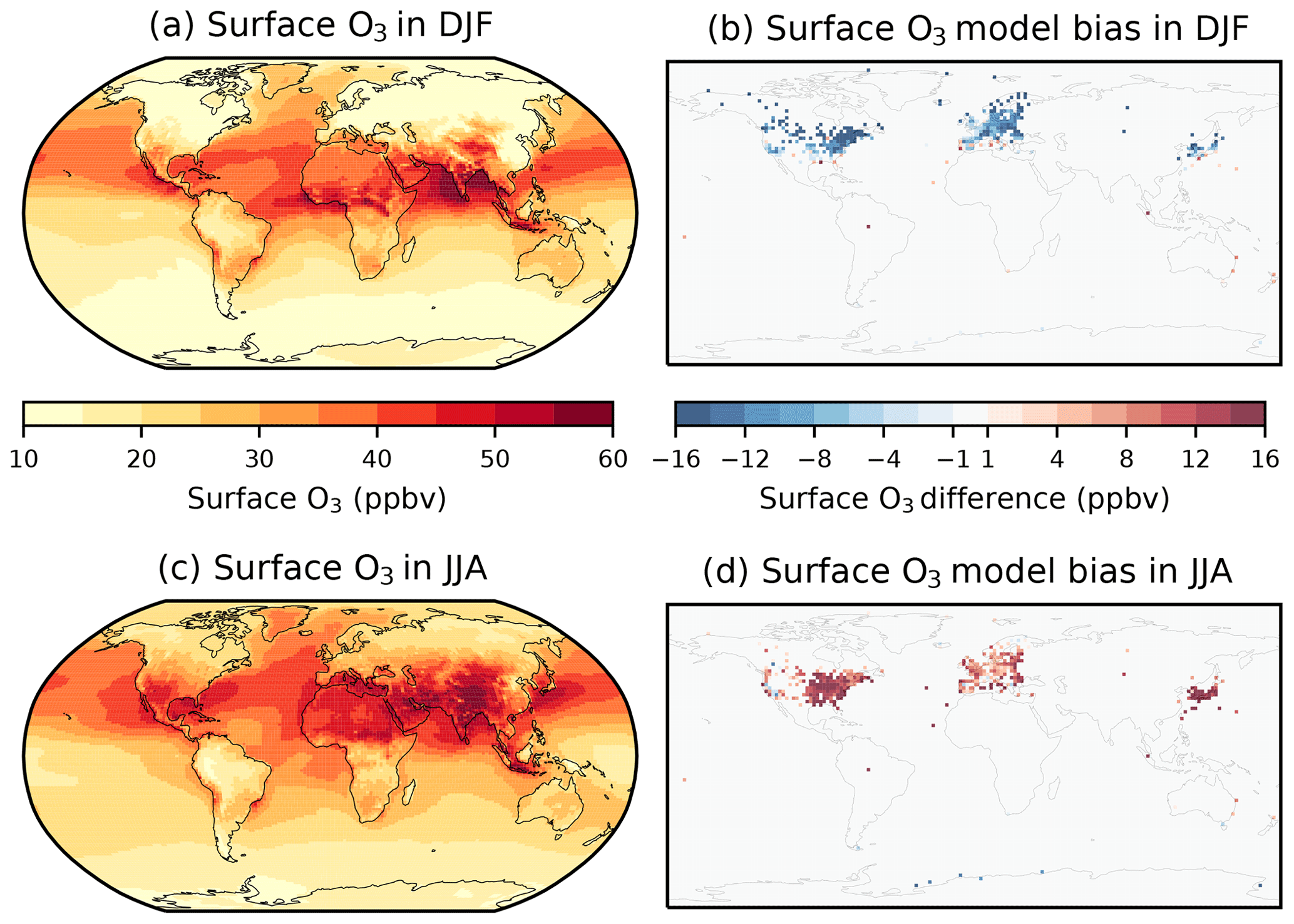
Figure 5 Simulated (ND) seasonal mean surface O₃ concentrations in (a) December–January–February (DJF) and (c) June–July–August (JJA) over the 2005–2014 period. Difference between simulated and observed surface O₃ from the gridded TOAR database in (b) DJF and (d) JJA.

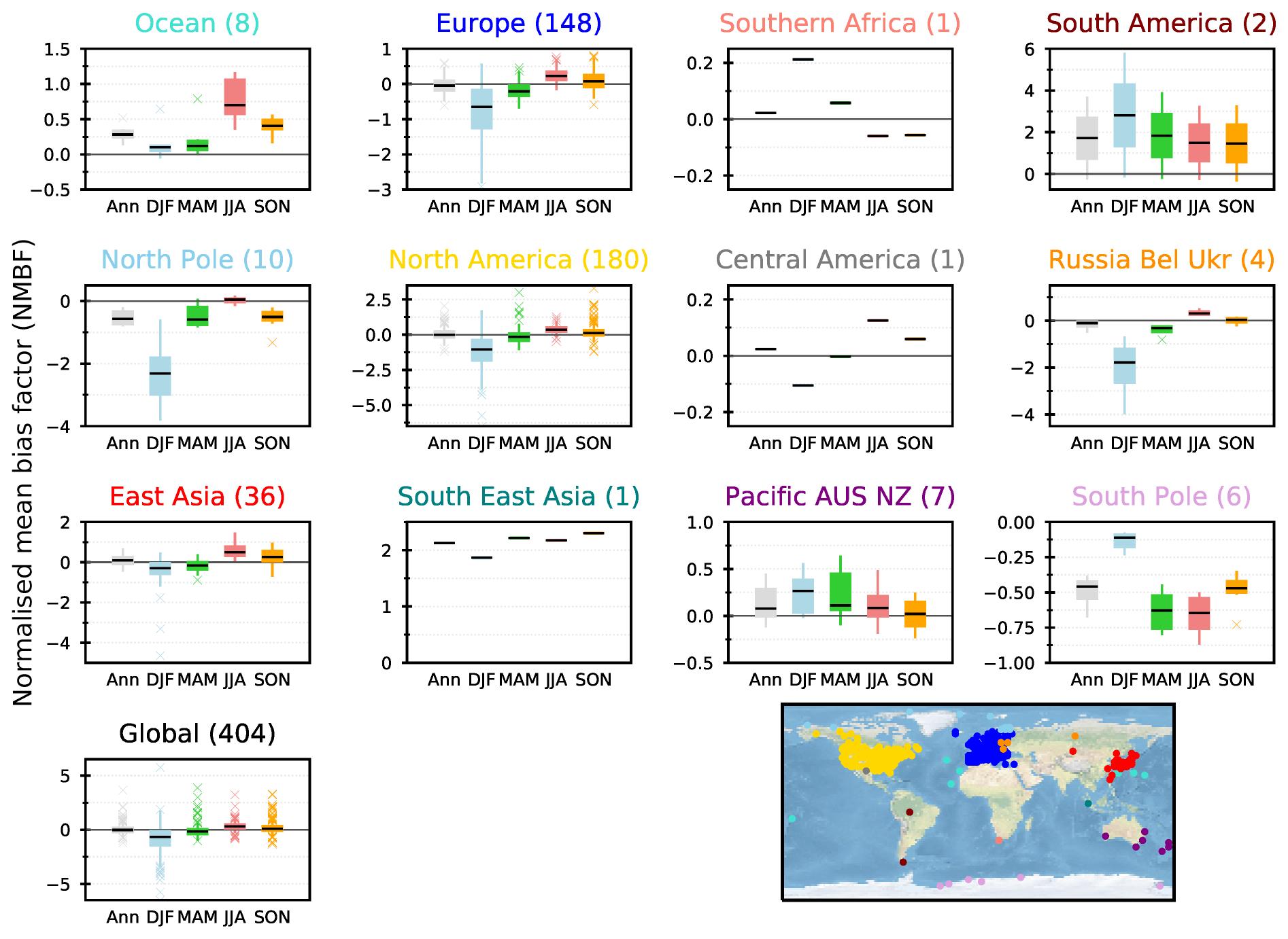
Figure 6 Normalised mean bias factors (NMBFs) calculated for annual and seasonal means by comparing modelled concentrations of surface O₃ in the UKESM1 ND simulations to gridded observations from the TOAR database across each region over the 2005–2014 period. The solid line shows the median value for the region, the boxes show the 25th and 75th percentile values (Q1 and Q3), with the error bars extending from the boxes to cover the main body of the data from (Q1 − 1.5 IQR) to (Q3 + 1.5 IQR) (IQR: interquartile range), and crosses represent outliers (values > 1.5 × interquartile range). The total number of sites used for each region is shown in parenthesis. Comparisons on annual (grey), DJF (blue), MAM (green), JJA (red) and SON (orange) timescales are shown.

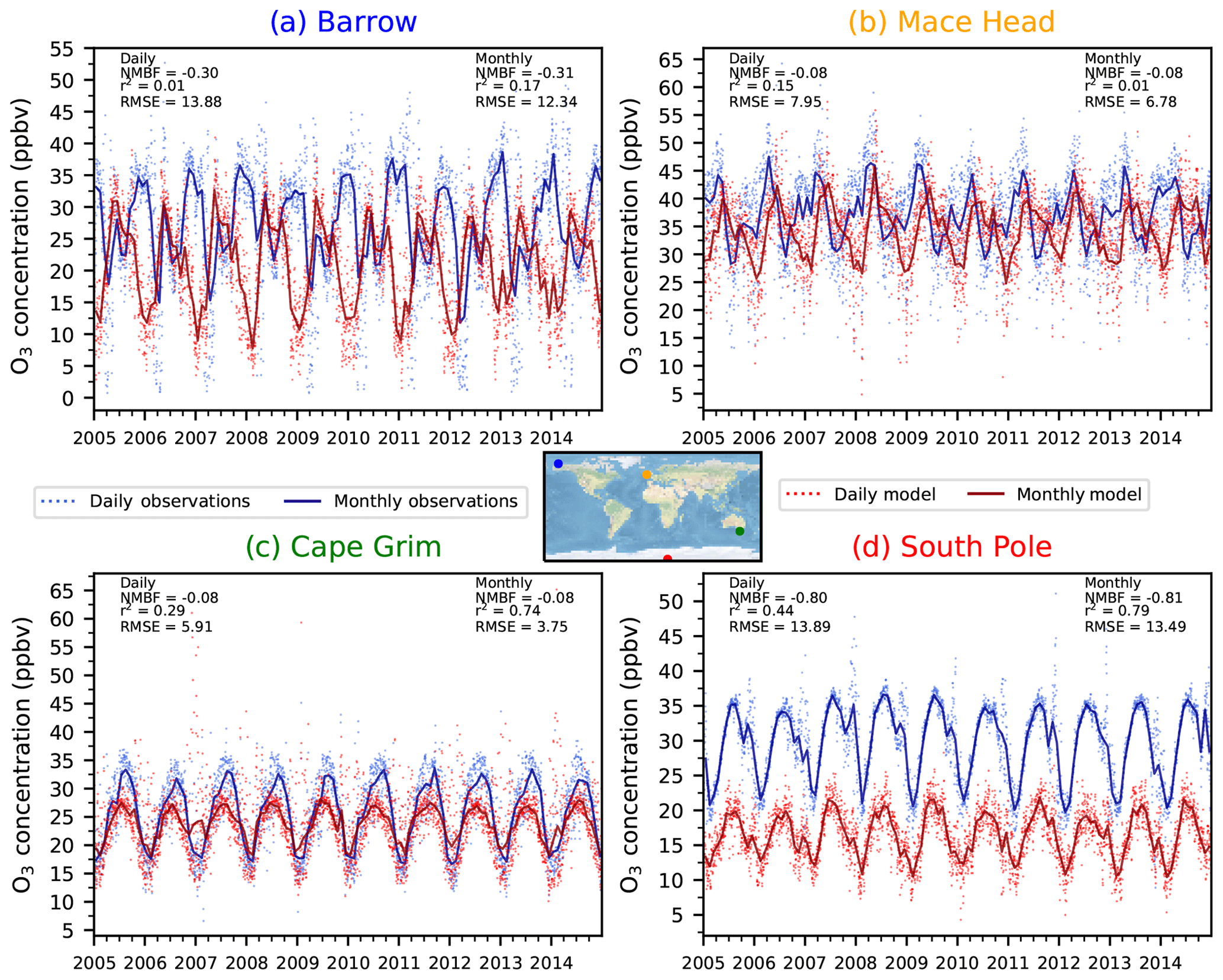
Figure 7 Simulated (ND) and observed daily and monthly mean surface O₃ over the period 2005–2014 at four individual monitoring locations of (a) Utqiagvik (formerly Barrow) (b) Mace Head, (c) Cape Grim and (d) the South Pole.

4.1 Evaluation of surface ozone against TOAR observations

The surface O₃ concentrations in the ND simulation with UKCA StratTrop in UKESM1 for December–January–February (DJF) and June–July–August (JJA) (seasonal means calculated from monthly means over the 2005–2014 period) show elevated values across the tropics in both seasons as well as in the northern mid-latitudes in JJA (Fig. 5a and c). Maximum surface O₃ concentrations of more than 60 ppb are simulated across the Middle East, northern Africa and South Asia in JJA due to large anthropogenic and biogenic sources of O₃ precursors. In DJF, surface O₃ concentrations are lower over the continental northern mid-latitudes due to slow O₃ production and an enhanced O₃ removal from elevated NO_x emissions. Meanwhile, surface O₃ concentrations are slightly higher over oceanic areas (North Atlantic and north-west Pacific) than over land in DJF, probably due to transport from the stratosphere and a reduced chemical sink from weaker photolysis of O₃ (Banerjee et al., 2016). Surface O₃ concentrations are slightly higher over some oceanic areas in JJA, indicating long-range transport from polluted continental areas.

Surface O₃ concentrations simulated in the nudged configuration of UKESM1 have been evaluated over the period 2005–2014 by comparing to the gridded monthly mean rural observations in the TOAR database over the same time period (Schultz et al., 2017). These data provide a global perspective on surface O₃ and are by far the most comprehensive surface O₃ database for use in the evaluation of global models. However, the TOAR database does not provide globally uniform coverage and as such the evaluation of the model performance for surface O₃ over key regions, such as South Asia (Hakim et al., 2019), will be analysed in more specific follow-up studies making use of bespoke datasets. Figure 5b and d show that the model underpredicts surface O₃ concentrations in DJF and overpredicts O₃ in JJA across the northern mid-latitudes, in a similar way as other global models (Young et al., 2018). Potential reasons for these discrepancies could be the coarse model resolution, associated errors in the emissions inventories, errors in the vertical injection of the emissions (for example, we inject most of the NO_x near the surface, which will titrate O₃), representation of VOCs in the chemistry scheme and uncertainties in O₃ loss processes (dry deposition).

Each grid point containing observations has been evaluated against the corresponding model values by calculating a normalised mean bias factor (NMBF; Yu et al., 2006). Figure 6 shows the distribution of NMBFs within a particular region for different seasons. Over northern mid-latitudes (Europe, North America and East Asia) the model clearly underrepresents surface O₃ in DJF (by a factor of 1.5 to 2), suggesting excessive O₃ titration by NO_x. The model agrees better with observations in other seasons across these regions, with a slight overprediction in JJA. The limited number of available observations in other regions (< 10 grid points) makes it difficult to draw firm conclusions but suggests that UKCA StratTrop in UKESM1 tends to overpredict surface O₃ across the oceanic and Southern Hemisphere sites. The model consistently underpredicts observed surface O₃ at sites located in Antarctica, implying a lack of transport and a modelled O₃ lifetime in this region that is too low, particularly in March–April–May (MAM) and JJA.

Simulated daily and monthly mean surface O₃ concentrations over the period 2005–2014 from UKESM1 have been interpolated and compared to four individual measurement locations from the TOAR database with daily and monthly mean observations (Fig. 7). UKESM1 is able to reproduce the seasonal cycle of surface O₃ observed at Cape Grim (r²=0.74 NMBF = −0.08) and the South Pole (r²=0.79, NMBF = −0.81), although it underestimates the magnitude in JJA at Cape Grim and in all seasons at the South Pole. There is reasonably good model–observation agreement in JJA at the two Northern Hemisphere sites (Utqiagvik, which was called Barrow, AK, until 2016, and Mace Head) (albeit with some disagreement in the phase), although in DJF the model underpredicts surface O₃ at both sites. The surface model evaluation of UKESM1 at selected individual measurement locations exhibits a similar performance to that of HadGEM2-ES in O'Connor et al. (2014).

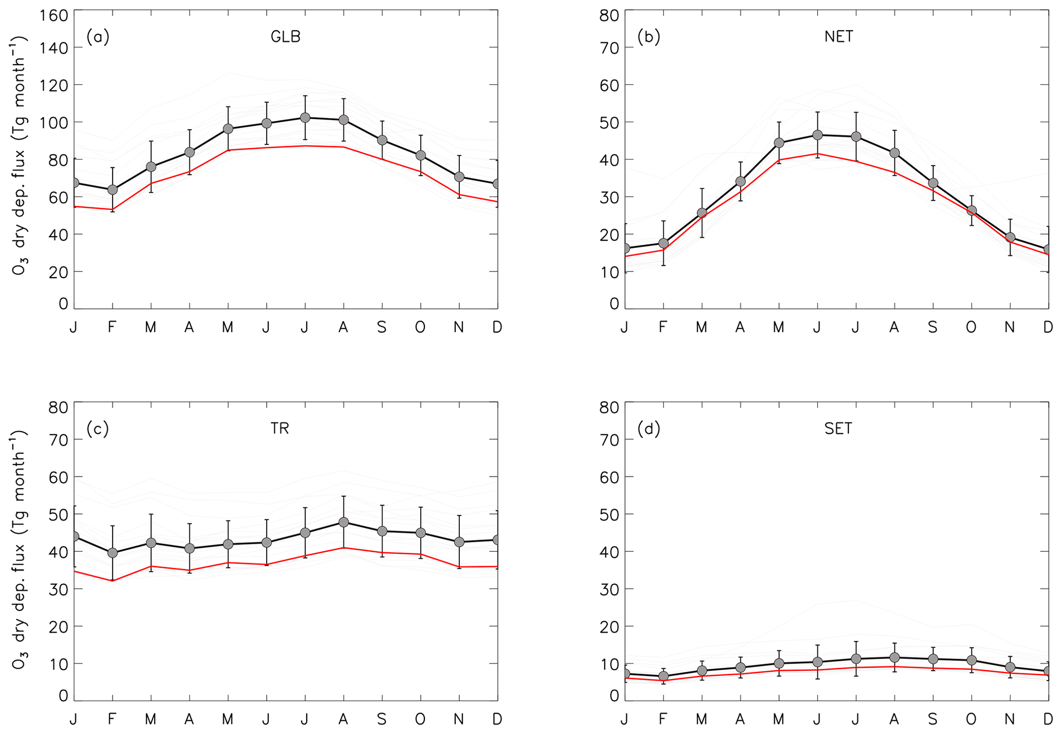
Figure 8 Multi-annual average monthly mean O₃ dry deposition fluxes for the global domain (a) and three latitudinal sections (b–d) for 15 models participating in the HTAP model intercomparison: northern extratropics (NET; 90–30^∘ N; b), tropics (TR; 30^∘ N–30^∘ S; c) and southern extratropics (SET; 30–90^∘ S; d). The multi-model ensemble average (solid black line and filled circles) and single-model monthly means (grey solid lines) were provided by Hardacre et al. (2015). Error bars indicate ±1σ in the single-model monthly means. The solid red line shows UKCA ND StratTrop multi-annual average (2005–2014) monthly mean O₃ dry deposition fluxes (figure based on Hardacre et al., 2015).

4.2 Dry deposition of ozone – comparison with HTAP models and observations

A total of 1030 Tg (O₃), around 20 % to 25 % of the gross chemical ozone production in the troposphere, is removed from the atmosphere in the ND simulation through dry deposition at the surface (Stevenson et al., 2006; Wild, 2007; Young et al., 2013; Hardacre et al., 2015). Uptake by terrestrial vegetation plays a crucial role; however, Hardacre et al. (2015) demonstrated that the oceans also represent a very important sink. Much uncertainty still remains about the exact magnitude and many of the processes around ozone removal at the surface (e.g. Hardacre et al. 2015; Luhar et al., 2017). A thorough evaluation and, if necessary, recalibration of ozone dry deposition models are thus critical in developing robust models of atmospheric composition.

Table 3 Ozone surface dry deposition measurement sites (reproduced from Hardacre et al., 2015).

(1) Fowler et al. (2001); (2) Fares et al. (2010); (3) Cieslik (2004); (4) Fares et al. (2012); (5) Fares et al. (2014); (6) Stella et al. (2011); (7) Munger et al. (1996); (8) Rannik et al. (2012); (9) Fan et al. (1990); (10) Mikkelsen et al. (2004, 2000); (11) Gerosa et al. (2007).

4.2.1 Comparison with the HTAP multi-model ensemble ozone deposition fluxes

Figure 8 shows a comparison of multi-annual average monthly mean ozone deposition modelled by UKCA StratTrop in UKESM1 with a multi-model ensemble of 15 HTAP atmospheric composition models (Hardacre et al., 2015). The StratTrop model data here are taken from the ND simulation. Monthly mean ozone deposition is depicted for the entire global domain (Fig. 8a) and split into the northern extratropics, the tropics and the southern extratropics, respectively, each representing a distinctly different deposition regime (Fig. 8b–d). The solid black line and filled circles represent ensemble average monthly mean ozone deposition, with the error bars indicating ±1σ in the single-model monthly mean ensemble; the solid grey lines represent single-model monthly means from the HTAP models, indicating the spread in the multi-model ensemble. The multi-annual average (10 years) monthly mean ozone dry deposition flux modelled by UKESM1-UKCA is shown as the red solid line.

In general, ozone dry deposition from UKCA StratTrop in UKESM1 compares favourably with the HTAP multi-model ensemble, nearly always falling within the 1σ range of the HTAP multi-model average. UKCA StratTrop also correlates well with the multi-model average seasonal cycle for each of the depicted regions; however, a systematic low bias is evident, particularly in the global and tropical domains (panels a and c in Fig. 8). Most of the low bias occurs in the tropical region. Since the tropics are dominated by both a large ocean surface area and the most productive portion of the Earth's terrestrial vegetation in the form of the tropical rainforests of South America, equatorial Africa and the Maritime Continent, the tropical low bias in the model could be due to an underestimation of O₃ concentration, the stomatal ozone uptake by tropical rainforests or a similar underestimation of O₃ removal at the ocean's air–sea interface. The latter seems less likely in view of the relatively good performance in the southern extratropics, which are also dominated by a large ocean surface.

4.2.2 Comparison with observations of ozone deposition fluxes

Measurements of ozone dry deposition fluxes collected over extended periods of time are still very sparse; however, a number of long-term datasets exist. Hardacre et al. (2015) compiled a comprehensive dataset from available long-term and short-term observations. This comprehensive dataset has been adopted for our evaluation of O₃ dry deposition in UKCA StratTrop in UKESM1. Table 3 summarises the locations of all the measurement sites included in this comparison. A comparison of the dry deposition fluxes of ozone with observations at these 16 sites is presented in Fig. 9. Some sites cover the seasonal cycle over several years (e.g. Castel Porziano, Harvard Forest, Ulborg) and others only offer data spanning less than 1 month (e.g. Klippeneck, Le Dezert, Viols en Levant).

Due to its removal via stomatal exchange and relative insolubility in water, O₃ dry deposition depends strongly on the underlying land surface type. Therefore, a reliable representation of ozone dry deposition in models requires not only the composition model to perform well. A robust model of the land surface including dynamic vegetation is also indispensable. The land surface representation in UKCA StratTrop in UKESM1 relies on JULES (Best et al., 2011; Clark et al., 2011). Thus, a comparison of ozone dry deposition (or any dry deposition process for that matter) reflects on the broader Earth system framework than just the atmospheric composition component alone.

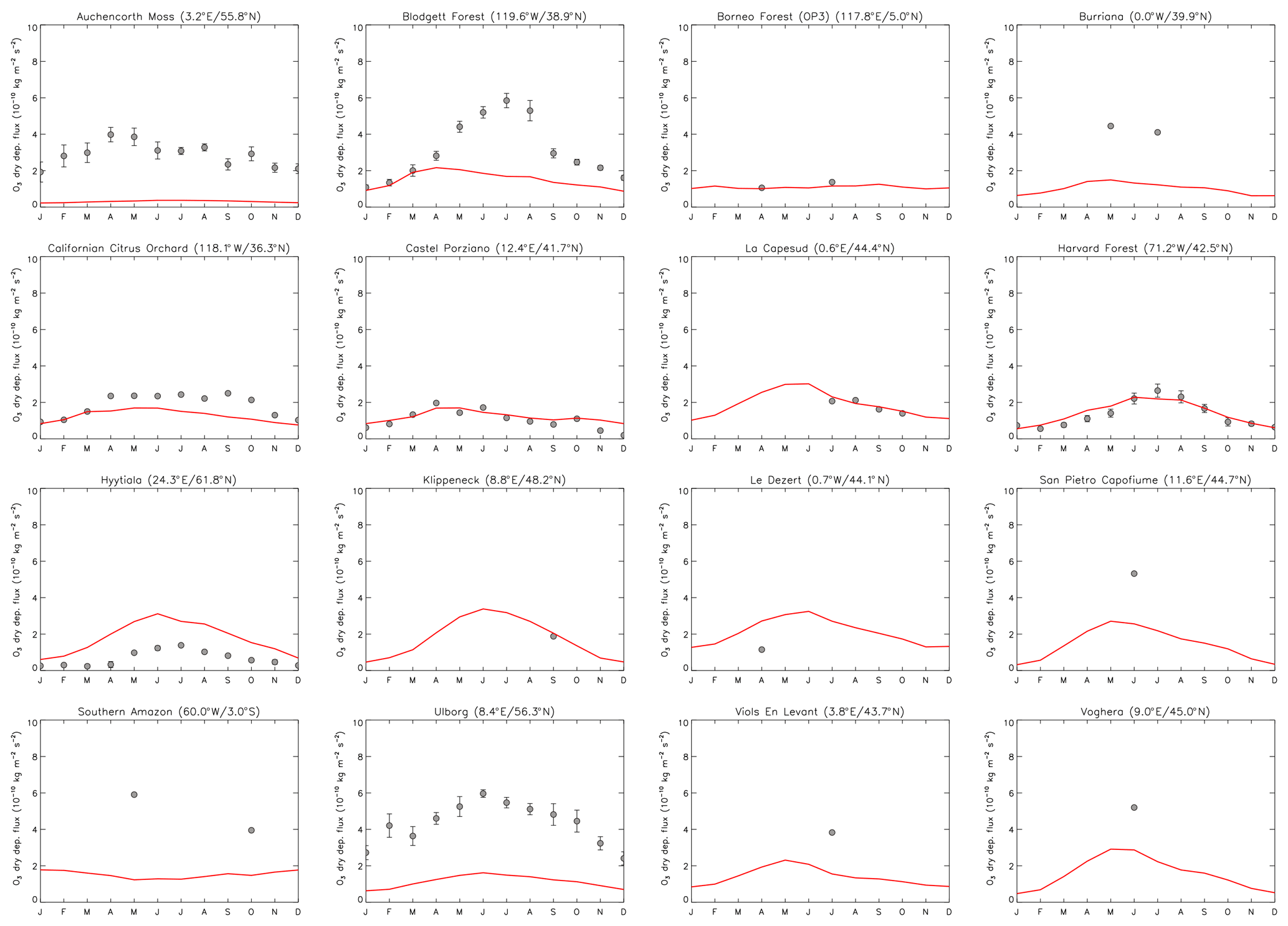
Figure 9 Comparison of observed and modelled monthly mean ozone dry deposition fluxes. Grey circles indicate monthly mean ozone deposition fluxes at measurement sites (see Table 3 for site details); error bars denote standard errors. Solid red lines represent modelled multi-annual average monthly mean O₃ deposition fluxes extracted from UKCA StratTrop ND in UKESM1 at the site locations by interpolation of the nearest grid boxes (averaged over all surface tiles in these grid boxes). Ozone dry deposition fluxes are given in 10⁻¹⁰ kg m⁻² s⁻¹, and measurement data are from Hardacre et al. (2015) and references therein.

Overall, Fig. 9 demonstrates that the UKCA(StratTrop)/JULES/UKESM1 framework shows a reasonably good performance, albeit with some substantial model-to-observation deviations evident. At the Castel Porziano, La Cape Sud and Harvard Forest sites the model reproduces both magnitude and seasonal cycle of ozone dry deposition well. To a somewhat lesser degree the model performance is also good at the California Citrus Orchard and Hyytiälä sites. At both locations the model captures most of the seasonal cycle well but fails to reproduce the magnitude of the flux fully. Interestingly, there is no systematic bias in the model-to-observation deviations with respect to magnitude and land cover type.

Further locations with good model-to-observation agreement include the densely forested OP3 site in Borneo and the Klippeneck site in Germany. However, these sites only provide campaign data for a limited period of time. The model shows very low skill in reproducing either the magnitude or seasonal cycle at three sites with long-term observational records, namely Auchencorth Moss (Scotland, UK), Blodgett Forest (California, USA) and Ulborg (Denmark). In all three cases the model severely underestimates O₃ dry deposition fluxes. The model also shows a fairly low skill in reproducing the seasonal cycle at these three sites. Potential reasons for the low model skill at these long-term observation sites include modelled surface ozone levels, deposition velocities and the appropriateness of the vegetation type, but more detailed analysis is required to explore these further. However, by and large, the model performance appears reasonable when compared to both observations and other models, although with an overall negative bias.

4.3 Model-simulated methane and OH

Here we discuss the performance of UKCA StratTrop modelled methane and tropospheric OH distributions. OH is the primary oxidising agent in the troposphere and is the key determinant on the burden of methane in the troposphere (Monks et al., 2015).

A commonly cited indicator of tropospheric oxidising capacity, the tropospheric lifetime of methane with respect to OH, has been calculated for the FR simulation, averaged over the entire length of the run. The modelled average tropospheric mean methane lifetime with respect to OH oxidation is calculated to be 8.5 years (with a standard deviation of 0.1 years). This value is in good agreement with the ACCMIP ensemble average of 9.7±1.5 years (Naik et al., 2013) (i.e. falling within 1 standard deviation of the ACCMIP ensemble). We note that the methane lifetime for UKESM1 is much shorter than the methane lifetime for HadGEM2-ES. Figure 4 shows this is largely down to improvement in the treatment of photolysis since HadGEM2-ES (Telford et al., 2013).

We further focus our analysis on comparing the climatological distribution of OH as a function of latitude and altitude (Fig. 10).

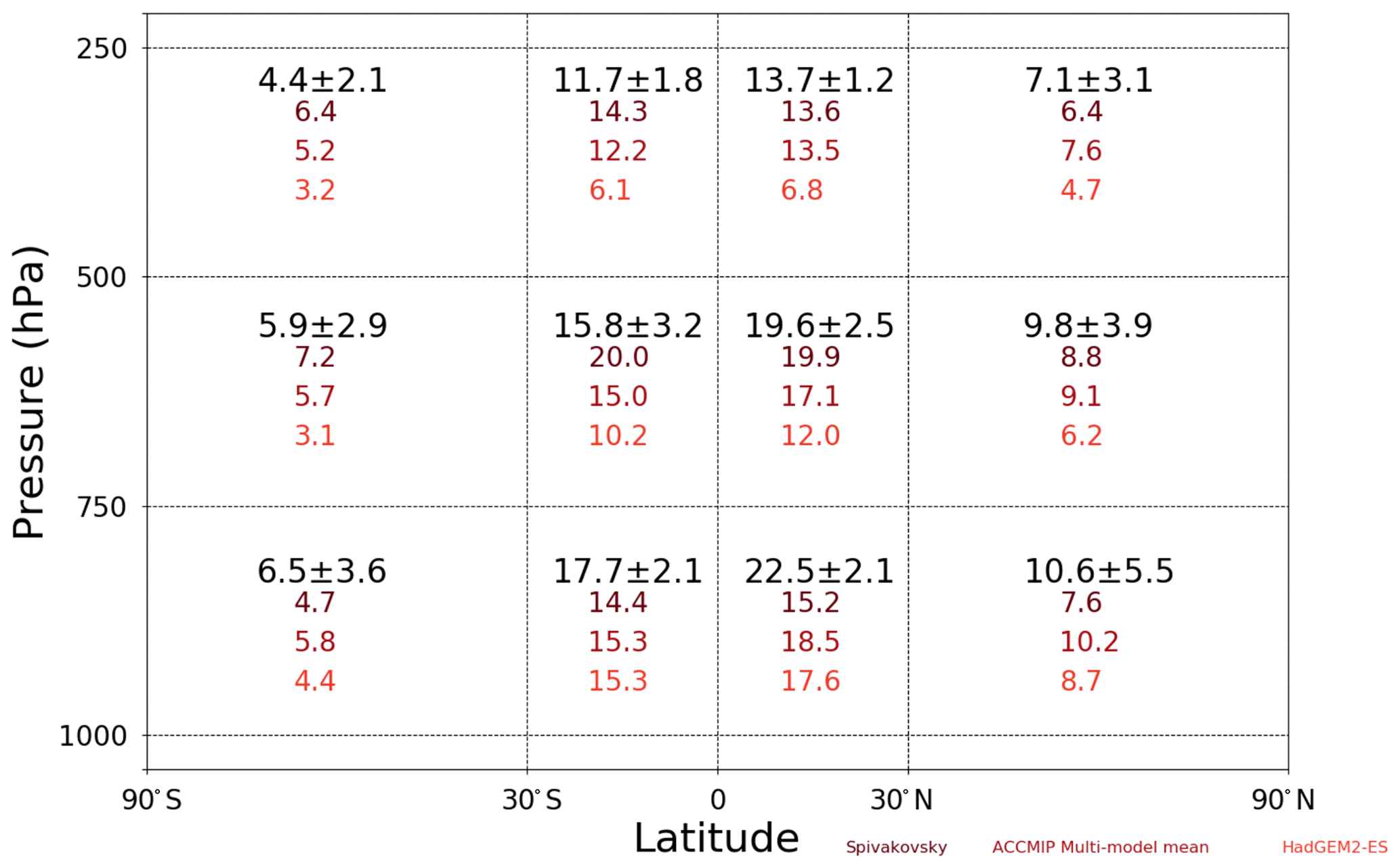
Figure 10 Evaluation of the UKCA StratTrop zonal distribution of tropospheric [OH] (×10⁵ molecules cm⁻³) in the FR simulation. Values plotted in black refer to the UKCA StratTrop multi-annual mean [OH] in each region of latitude and pressure range, with the values following being ±1 standard deviation around the mean.

The FR UKCA StratTrop simulation results in a global mean tropospheric [OH] of 1.22×10⁶ molecules cm⁻³, averaged over the period 2005–2014. As with the methane lifetime, this value is slightly higher than the ACCMIP ensemble mean ($\mathrm{11.1}\pm \mathrm{1.6}\times {\mathrm{10}}^{\mathrm{5}}$ molecules cm⁻³) but sits within the standard deviation of the ACCMIP ensemble mean (Naik et al., 2013). Figure 10 shows how the distribution of [OH] varies throughout the troposphere relative to the ACCMIP multi-model mean, the HadGEM2-ES model and the data from Spivakovsky et al. (2000), who pioneered the development of [OH] climatologies in the troposphere. Compared against these data, UKCA StratTrop in UKESM1 performs well: the global tropospheric mean [OH] is within 10 % of the ACCMIP ensemble mean. The model captures the latitudinal and vertical profiles found in the other datasets and agrees on the magnitude of [OH] in 10 of the 12 regions analysed (when considering the model uncertainty).

The [OH] is higher in UKCA StratTrop than in HadGEM2-ES, partly because of different emissions used in the HadGEM2-ES study, but also in part owing to the change in photolysis scheme (as discussed previously). UKCA StratTrop agrees better with the ACCMIP multi-model mean than Spivakovsky or HadGEM2-ES, but the tropics from 1000 to 750 hPa are regions where the model consistently disagrees with the other datasets, simulating higher levels of OH in these regions. These regions of the troposphere are the regions where most CH₄ is oxidised, so high biases in the model here will tend to lead to lower CH₄ lifetimes than in observation-derived estimates.

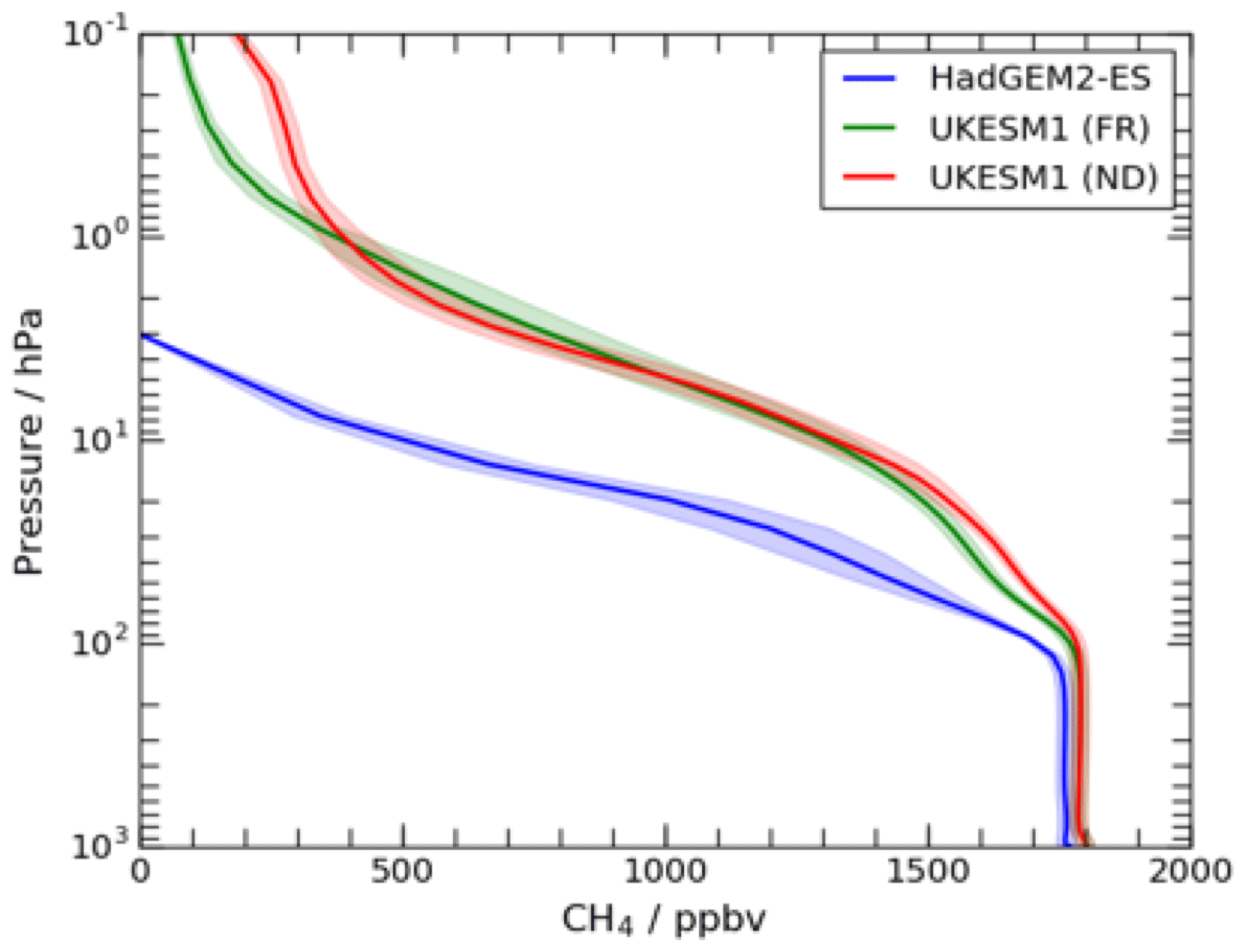
Figure 11 Vertical profiles of the mean tropical (±10^∘ N) modelled methane from multi-annual mean output from an atmosphere-only free-running simulation of HadGEM2-ES (OC14; blue), an atmosphere-only free-running FR (green) and nudged (ND; red) simulations of UKCA StratTrop in UKESM1 (this study). The shading represents ±1 standard deviation about the multi-annual mean.

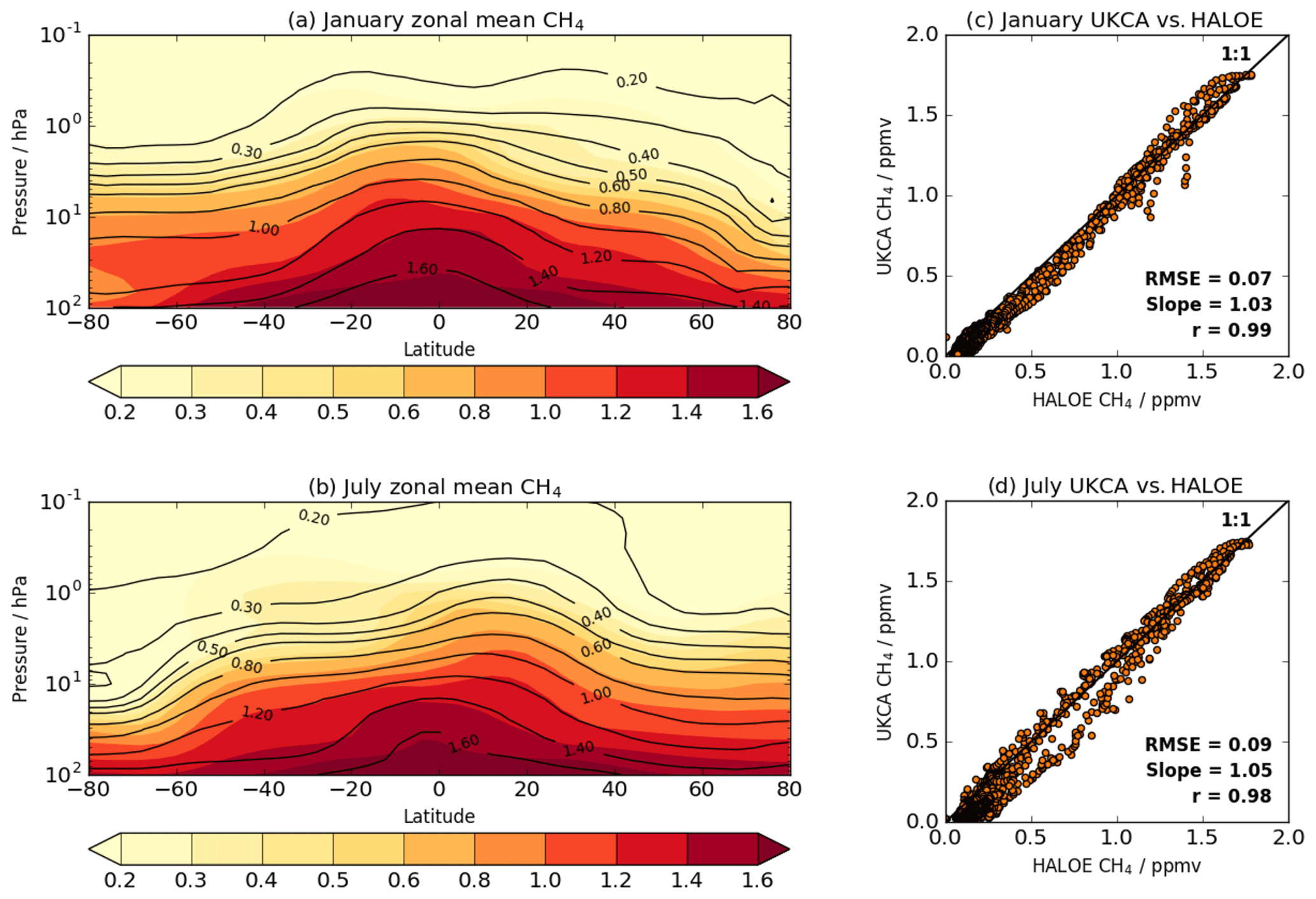
Figure 12 Multi-annual (2005–2014) monthly zonal mean methane (ppm) from the UKESM1 FR simulation in (a) January and (b) July, with scatter plots of modelled versus observed concentrations for January and July in panels (c) and (d), respectively. The coloured contours in (a) and (b) are from UKCA and the black contours are the HALOE/CLAES climatology. The scatter plots also include a 1 : 1 line as well as the root mean square error (RMSE), the slope of a least squares linear fit and the correlation coefficient (r).

In the previous configurations of UKCA (MO09 and OC14), methane concentrations fell off too quickly with height above the tropopause; this was attributed to the stratospheric transport timescale being too long in the respective physical model. Comparisons of methane columns from the HadGEM2-UKCA coupled model with SCIAMACHY, for example, were too low and required modelled methane above 300 hPa to be overwritten with Halogen Occultation Experiment (HALOE; Russell et al., 1993) and Atmospheric Chemistry Experiment (ACE; Bernath et al., 2005) assimilated output from TOMCAT (Hayman et al., 2014). Figure 11 shows that the fall-off of methane with height in both the FR and ND simulations of UKESM1 is less rapid than in HadGEM2 and is consistent with the age of air in the model being comparable to that inferred from observations (Sect. 4.6). As comparisons with surface observations and SCIAMACHY (with its strong sensitivity to surface concentrations) are not appropriate here because surface methane concentrations are relaxed to LBCs (Sect. 2.6.4), only comparisons with stratospheric observations are shown.

Figure 12 shows multi-annual zonal mean comparisons for January and July of modelled methane from the free-running (FR) simulation against the HALOE/Cyrogenic Limb Array Etalon Spectrometer (CLAES) climatology (Kumer et al., 1993). It indicates that UKCA StratTrop in UKESM1 is capable of simulating the absolute concentrations and the morphology of the observed distribution. The only exception to this is the tongue of methane-depleted air descending from the mesosphere over the SH high latitudes in July, which was also evident in MO09. Nevertheless, UKESM1 is able to capture the observed vertical fall-off with height. There is an excellent 1 : 1 correspondence between the model and observations: the slopes of the least squares fits for January and July are within 0.05 of unity, the correlation coefficients are greater than 0.98, and the root mean square errors between UKESM1 and the HALOE/CLAES climatology are less than 0.1 ppm for the free-running (Fig. 12) and nudged (not shown) simulations.

4.4 Comparison of total ozone column

Here we discuss the modelled total ozone column through an analysis of the data from the FR simulation averaged over the 2005–2014 period. We note here that there is little difference between the ND and FR total column, so for simplicity we focus on the FR data.

Figure 13a shows the multi-annual average total ozone column in Dobson units as a function of latitude and time. As with most chemistry–climate models (Dhomse et al., 2018), UKCA simulates the main features of the total column well, with a minimum in the tropics and maxima at high latitudes during the hemispheric spring seasons. When compared with the total-column ozone in older versions of UKCA (M09, Fig. 9) the current model configuration simulates similar biases at high latitudes but a pronounced positive bias in the tropics. Figure 13b highlights that the tropical column is biased high by 30–40 DU when compared to the Bodeker climatology (Hassler et al., 2008), and the Antarctic ozone hole extends for too long in the model, leading to low biases in the austral summer. The high biases in total-column ozone in the tropics are very likely driven in part by high biases of around 15 DU in the tropical tropospheric ozone column (see Sect. 4.5 below). The extratropical biases may well be related to this bias through the transport of ozone-rich air in the upper troposphere–lower stratosphere (UTLS) into this region, but further work is needed to resolve the causes of the bias in the total ozone column.

Figure 13 Evaluation of the FR UKCA total ozone climatology. Panel (a) shows the FR simulation multi-annual mean total-column ozone climatology (in Dobson units – DU). Panel (b) shows the difference between the FR ozone climatology and the Bodeker ozone climatology v2.8.

4.5 Comparisons with satellite retrievals of tropospheric columns of O₃, CO and NO₂

Here we compare the results from the UKCA StratTrop runs against satellite data with a focus on assessing performance in the troposphere. In all cases, the run analysed is the nudged dynamics (ND) run discussed in Sect. 3. Nudging enables a more robust comparison against the satellite observations as it reduces biases caused by circulation errors in the free-running model, although we note that it does not completely remove these biases (Orbe et al., 2018; Chrysanthou et al., 2019). As well as nudging, the model output is sampled instantaneously every 3 h to allow for time and space sampling to the satellite data locations. The comparison between the model and the observations is made using OMI-MLS for the tropospheric column of O₃, MOPITT for the tropospheric column of CO and OMI for the tropospheric column of NO₂.

In the following analysis, the stratosphere has been removed by screening out regions where the monthly mean ozone exceeded 125 ppb, the ozonopause; columns are calculated by summing variables from the surface to the height at which the ozonopause starts. The model ozone data presented here have not been corrected to account for optically thick clouds in the troposphere, which may affect retrieved ozone profiles (Ziemke et al., 2006) since averaging kernel (AK) information is not available for the OMI-MLS dataset. As satellite measurement errors were not available, we have used 2 times the standard deviation of the retrievals to estimate when the differences between modelled and observed ozone are significant. This implies that the stippling area in the plots, corresponding to grid cells in which |model bias| > satellite error, could be reduced (i.e. better agreement with the observations) if the satellite error is added to the 2×SD. The plots therefore show a “worst-case scenario”.

Figure 14 Comparison of observed and modelled tropospheric ozone columns (DU) from the ND simulations. Plots show seasonal means and differences for the period 2005–2014. (a) OMI-MLS tropospheric column (DJF); (b) difference between the model nudged simulations and OMI-MLS tropospheric column (DJF); (c) OMI-MLS (JJA) tropospheric column; (d) difference between the model and OMI-MLS tropospheric column (JJA). Stippling indicates grid points for which |bias| > 2×SD of the observations.

The model fields have been co-located in time and space with the observations to reduce representation errors. For each satellite retrieval, the nearest model grid box is subsampled within 3 h of the observation and the model profile interpolated onto the satellite pressure grid. The satellite AKs (where available) are then applied to the model profile to account for the vertical sensitivity of the instrument. Then the model sub-columns are calculated and summed between the surface and the tropopause to determine the co-located model tropospheric column. The equations used to apply the OMI NO₂ and MOPITT CO AKs to the model profiles are

$$\begin{array}{}\text{(10)}& {\displaystyle }& {\displaystyle }y=A\cdot x,\text{(11)}& {\displaystyle }& {\displaystyle }y={\mathrm{10}}^{\left(A\right(\log \mathrm{10}\left(x\right)-\log \mathrm{10}\left(x_{\text{a}}\right))+\log \mathrm{10}(x_{\text{a}}\left)\right)},\end{array}$$

where x is the co-located model profile interpolated onto the satellite pressure grid, A is the satellite averaging kernel, x_a is the satellite a priori and y is the modified model profile. Here x for NO₂ is in sub-columns (units: 10¹⁵ molecules cm⁻²), while x for CO has units of volume mixing ratio (vmr) before conversion into a ratio of sub-columns to the tropospheric column. Tropopause height information was provided by the OMI NO₂ files, but for MOPITT-derived tropospheric column CO we use the climatological tropopause described by Monks et al. (2017).

The modelled tropospheric ozone column (TC_O3) is evaluated against the OMI-MLS tropospheric ozone column (Ziemke et al., 2006). The general agreement between UKCA StratTrop and OMI-MLS is good and in line with many other CCMs (Young et al., 2013). A general feature of the model is a small underestimation in the tropospheric ozone column in the Southern Hemisphere extratropics, generally good agreement in the Northern Hemisphere extratropics and significant positive biases of 15 DU in the tropics (Fig. 14). The underestimation in tropospheric ozone in the southern mid-latitudes is worse in the late summer and early autumn when OMI-MLS shows a seasonal maximum in the Southern Hemisphere that the model fails to reproduce (Fig. 15c).

For the northern mid-latitudes, Fig. 14b shows that in DJF the model overestimates tropospheric ozone over large parts of the North Atlantic Ocean while underestimating it over northern Russia and large parts of the North Pacific Ocean. These two biases counteract each other in the time series plot (Fig. 15a) to give good net agreement overall. It is worth noting that the time series plots show that there are very small, if any, trends in tropospheric column ozone when averaging across these large domains. Figures 14d and 15a show that in JJA the model biases in the northern mid-latitudes are generally very small, and the amplitude and phase of the modelled seasonal cycle are in good agreement with the OMI-MLS data. In the tropics the differences shown in Fig. 14b and d are around 25 %–50 %. There are potentially several causes for this including (a) the representation of chemistry in this region, (b) the underlying emission inventories, (c) the deposition rates (which are on the low end compared with other models) and (d) the emissions of ozone precursors. The pattern of the bias strongly resembles patterns in the emissions of NO_x from lightning. It has been noted before that the modelled tropospheric ozone is extremely sensitive to the average global NO_x emitted by lightning, which is mainly centred around the tropics. The model bias in the tropics might be a result of the simplified parameterisation of lightning NO_x emissions, and further work will focus on reducing this bias.

Figure 15 Tropospheric column O₃ (DU) zonal time series (30–60^∘ N – a, 30^∘ N–30^∘ S – b, 30–60^∘ S – c) for the ND simulation (red) and OMI-MLS (black). Dashed lines represent the satellite uncertainty range ($\pm \mathrm{2}\times \text{SD}$).

Figure 16 Comparison of observed and modelled tropospheric CO columns (DU) from the ND simulations. Plots show seasonal means and differences for the period 2005–2014. (a) MOPITT tropospheric column (DJF); (b) difference between the model and MOPITT tropospheric column (DJF); (c) MOPITT (JJA) tropospheric column; (d) difference between the model and MOPITT tropospheric column (JJA). Stippling indicates grid points for which |bias| > satellite error.

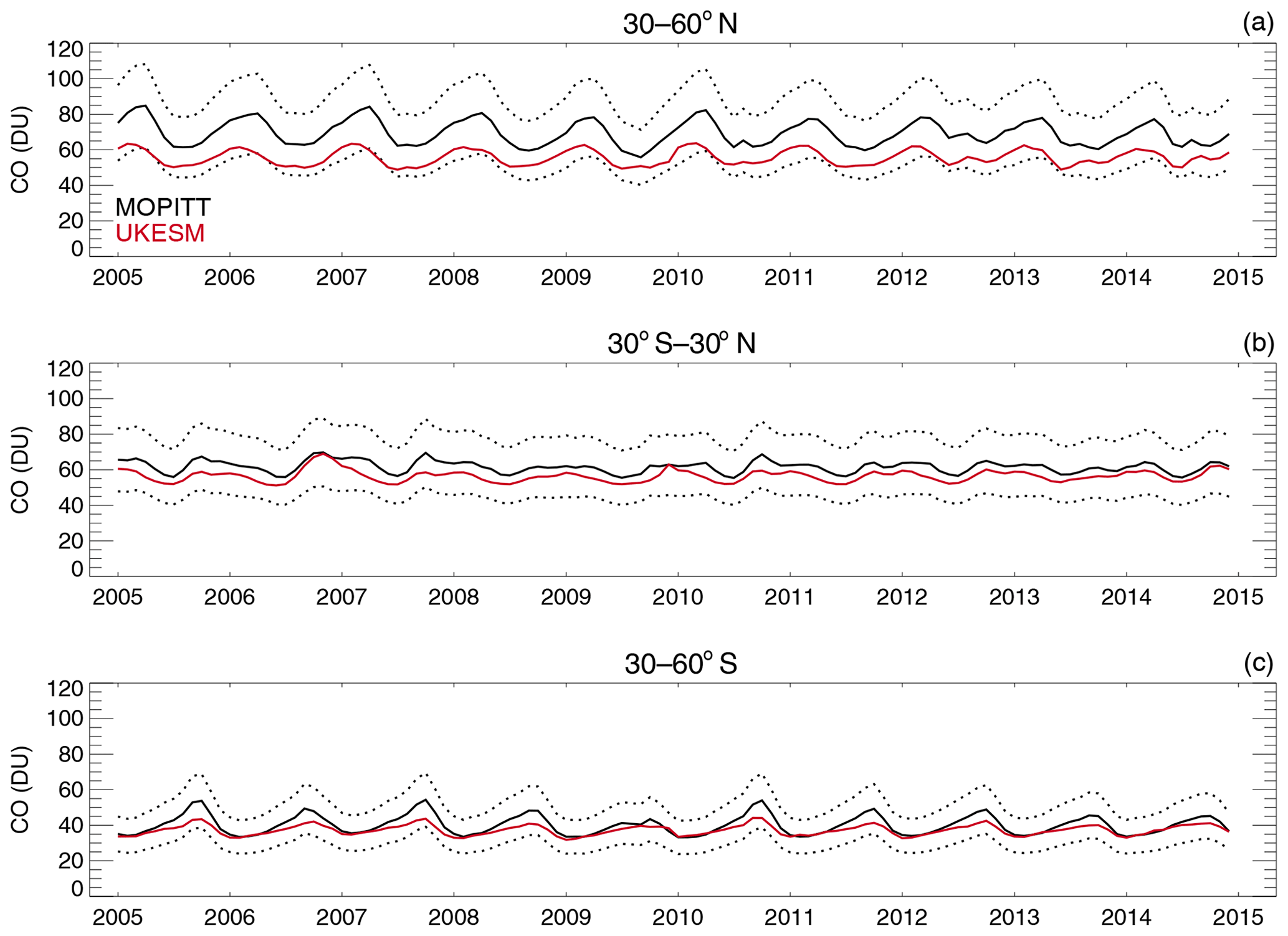
Figure 17 Tropospheric column CO (DU) zonal time series (30–60^∘ N – a, 30^∘ N–30^∘ S – b, 30–60^∘ S – c) for the ND simulation (red) and MOPITT (black). Dashed lines represent the satellite uncertainty range.

Figure 16 shows a comparison of the tropospheric column of CO in the UKCA StratTrop nudged dynamics runs with retrievals from the MOPITT instrument onboard Terra (Emmons et al., 2004). The MOPITT data reveal that the tropospheric column CO (TC_CO) is highest over anthropogenic and biomass burning emission regions and lowest over the remote oceans. There is a strong north–south gradient which is set up from the short lifetime of CO (∼ 30 d) and the timescales for interhemispheric mixing. (NB Fig. 16a highlights strong emissions of CO in DJF in the northern mid-latitudes). The general feature evident from Fig. 16 is that the model significantly underestimates TC_CO in the Northern Hemisphere (NH) in both winter and summer. The negative bias in TC_CO is especially large at high northern latitudes, consistent with surface CO biases in this region (e.g. Shindell et al., 2006). Whilst the NH shows a negative bias, there is a strong positive bias in CO in regions associated with agricultural (Indo-Gangetic Plains) and forest burning (central Africa and northern South America).

There are a number of reasons for the model–satellite biases in TC_CO, including (1) CO emissions in the NH being underestimated (Miyazaki et al., 2015), (2) insufficient secondary production of CO from non-methane VOC oxidation (e.g. Grant et al., 2010), (3) excess biomass burning emissions in the Southern Hemisphere (SH) during DJF (potentially the same cause in central Africa in JJA) and (4) strong loss through OH in the NH in both seasons. We note that these types of biases are not unique to UKCA StratTrop and that further work is required to ameliorate them (Shindell et al., 2006).

As shown in Fig. 17, there is no clear trend in modelled and observed TC_CO over time. However, both datasets show seasonal cycles in TC_CO in the NH and SH with a very muted seasonal cycle in the tropics. The model simulations again underestimate (∼ 10–20 DU) TC_CO in the NH mid-latitudes but successfully capture the amplitude and phase of the seasonal cycle (albeit with a slightly smaller amplitude) and the magnitude of interannual variability well. In the Southern Hemisphere, the model is doing very well in capturing the absolute concentration, seasonal cycle and interannual variability, although it underestimates the peaks during the austral winter. There is also an underestimation of CO in the tropics despite the positive bias over biomass burning areas.

Figure 18 Comparison of observed and ND modelled UKCA StratTrop in UKESM1 tropospheric NO₂ columns (molecules cm⁻²). Plots show seasonal means and differences for the period 2005–2014. (a) OMI tropospheric column (DJF); (b) difference between the model and OMI tropospheric column (DJF); (c) OMI (JJA) tropospheric column; (d) difference between the model and OMI tropospheric column (JJA). Stippling indicates grid points for which |bias| > satellite error.

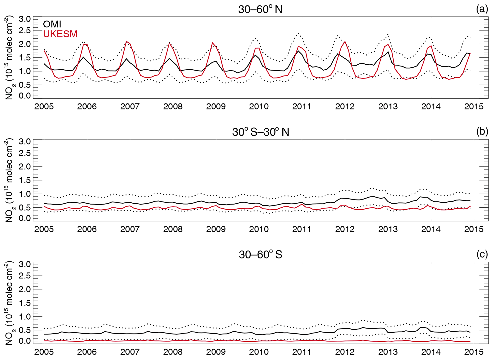
Figure 19 Tropospheric column NO₂ (10¹⁵ molecules cm⁻²) zonal time series (30–60^∘ N – a, 30^∘ N–30^∘ S – b, 30–60^∘ S – c) for the ND simulation (red) and MOPITT (black). Dashed lines represent the satellite uncertainty range.

Finally, we focus on the comparison of modelled and observed tropospheric NO₂ columns. The observed tropospheric NO₂ column (TC_NO2) data come from the OMI instrument onboard AURA (Boersma et al., 2011). The observed NO₂ column is highly heterogeneous and localised to the major industrialised regions, where anthropogenic emissions are highest, and major biomass burning zones (Fig. 18). The figure highlights strong seasonal differences in the observations, with TC_NO2 being larger in winter (panel a) than in summer (panel c), most likely as a result of higher emissions and a longer NO₂ lifetime than in the former season. Averaged across the whole troposphere, the model compares well with OMI TC_NO2 spatially (Fig. 18b, d). However, there are very significant positive biases over the main anthropogenic emission regions (i.e. South Asia, eastern Europe, East Asia and outflow from the US eastern seaboard), particularly in the boreal winter. These biases in TC_NO2 are only weakly correlated with the biases in TC_O3 in these regions, suggesting different causes, and they are dominant in different regions of the atmosphere (boundary layer vs. free troposphere). A high bias in TC_NO2 extends out from the North China Plain region, across the Sea of Japan and into the Pacific Ocean, suggesting either errors in the underlying emission inventory or in the modelled NO₂ lifetime.

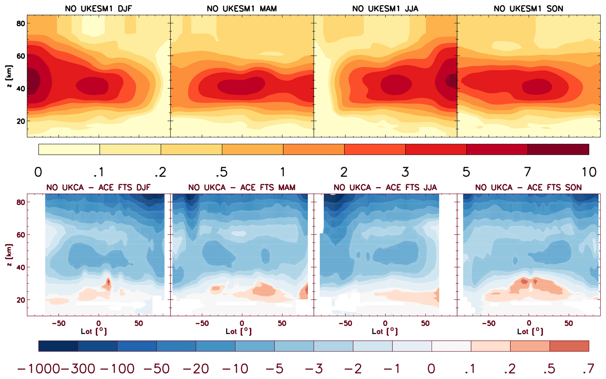
Figure 20 Zonal annual, seasonal annual, and multi-annual mean nitric oxide (NO) volume mixing ratio in parts per billion. Top row: UKCA StratTrop, February 2004 to February 2013. Bottom row: bias versus the ACE-FTS v3.5 climatology, with the same units and period. The climatology represents the average of sunrise and sunset measurements, while the model values are averaged over all local times. The model data analysed are from the FR simulation.

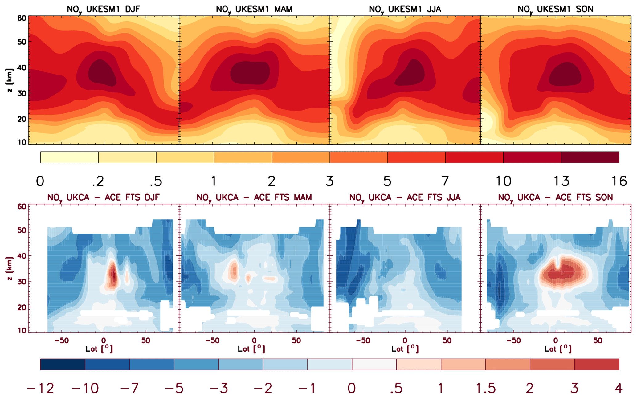
Figure 21 Same as Fig. 22 but for odd nitrogen (NO_y), defined here as ${\mathrm{NO}}_y=\mathrm{NO}+{\mathrm{NO}}_{\mathrm{2}}+{\mathrm{HNO}}_{\mathrm{3}}$ (ppb). For ACE-FTS, NO and NO₂ fields are the average of sunrise and sunset measurements. The model values are averaged over all local times.

Over biomass burning regions, there is evidence for low biases over central Africa and South America (mainly in JJA). This may well be a vertical sensitivity issue in the comparison of the datasets. As OMI has peak sensitivity in the middle to upper troposphere, OMI detects enhanced NO₂ values over biomass burning regions due to the buoyant fire plumes. In UKESM1, the gas-phase anthropogenic and biomass burning emissions are added to the surface level, so most of the NO_x will be trapped in the boundary layer where OMI is less sensitive. Therefore, the satellite AKs will give this sub-column less weighting and a negative bias occurs.

Figure 19 highlights that in both the model simulation and satellite data, the average Southern Hemisphere extratropical TC_NO2 is lower than in the Northern Hemisphere due to fewer emission sources. However, in the model there is a significant low bias in this region, ∼ 50 %. This bias is largest over the oceans and may be connected with biases in the representation of NO_y species (i.e. PAN), which are large contributors to NO_x in this region.

In the northern extratropics, the model-simulated TC_NO2 is within the observational uncertainty but with too large a seasonal cycle, the simulated mean annual minima and maxima being much lower and higher, respectively, than the observed mean annual minima and maxima.

4.6 Evaluation of zonal mean stratospheric composition

Sellar et al. (2019) provide an overview of the simulation of total-column ozone. Their results and ours (see Fig. 13) indicate that UKESM1 produces relatively realistic ozone fields, albeit with some remaining issues. Among these is a tendency for the Antarctic ozone hole to be too persistent, insufficiently variable and on average too deep. This is linked to a stratospheric cold bias noted before (Dennison et al., 2019).

In the analyses below, UKCA StratTrop seasonal and zonal mean composition fields from the FR simulation are compared to selected species from the Atmospheric Chemistry Experiment–Fourier Transform Spectrometer (ACE-FTS) climatology version 3.5. ACE-FTS is an ongoing satellite mission sponsored by the Canadian Space Agency; it uses solar occultation to observe a substantial number of species with a coverage extending in some cases into the mesosphere. The climatologies used here cover the period of February 2004 to February 2013 (http://www.ace.uwaterloo.ca/climatology_3.5.php, last access: September 2017). Here we focus on NO, NO_y (defined here as $\mathrm{NO}+{\mathrm{NO}}_{\mathrm{2}}+{\mathrm{HNO}}_{\mathrm{3}}$), CO, H₂O and O₃. Climatologies of N₂O₅ and ClONO₂ measurements by ACE-FTS are also available but are not included in the NO_y calculation presented here because of their more restricted coverages than the NO, NO₂ and HNO₃ climatologies. Both would contribute relatively minor amounts to NO_y compared to the large biases discussed below.

Figure 22 Same as Fig. 20 but for carbon monoxide (CO; ppm).

Figure 23 Same as Fig. 20 but for water vapour (H₂O; ppm).

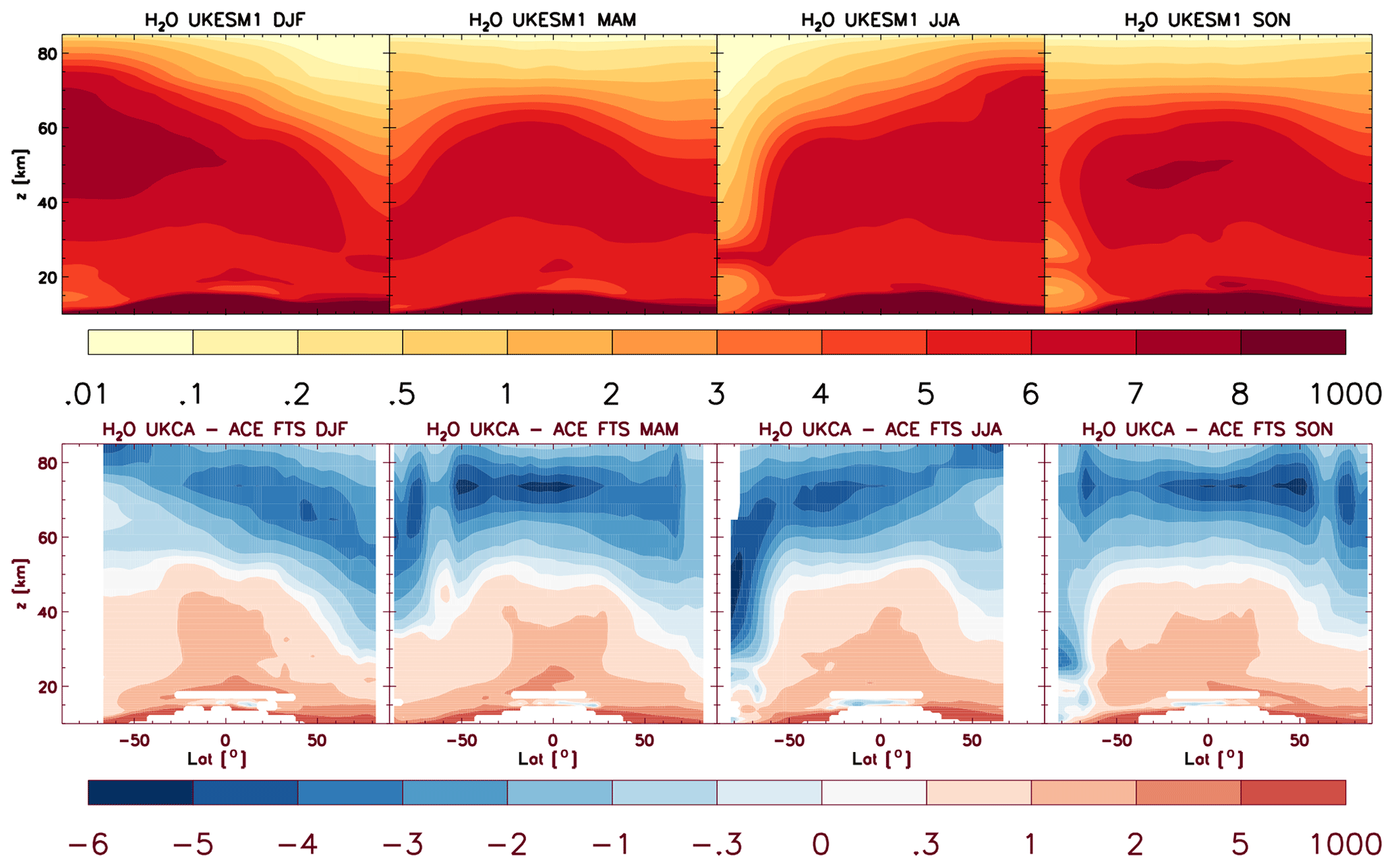
NO is underestimated throughout the model domain (Fig. 20). In the troposphere and much of the stratosphere, NO is subject to a large diurnal cycle. When exposed to sunlight it is maintained by photolysis but converts to NO₂ at night by reacting with O₃. However, near and above the top of the region covered by NO₂ measurements, at ∼ 50 km, this conversion becomes slow and NO is also the dominant form of nitrogen in the ACE-FTS measurements at night. This implies that the large underestimation of NO seen above 50 km, which reaches about 1 ppm, is not a sampling problem associated with imperfect spatio-temporal matching of satellite and model data. Rather, it reflects a model shortcoming. To illustrate the consequences of this issue for stratospheric composition, we compare NO_y (Fig. 21). This diagnostic reveals tongues of nitrogen-depleted air descending in the polar vortices of both hemispheres in the model, which in the ACE-FTS measurements are, however, relatively nitrogen-rich. This discrepancy lasts into southern spring when NO_y is underestimated by up to 12 ppb at around 70^∘ S. The depletion of HNO₃ due to denitrification in the lower Antarctic polar vortex appears to be well reproduced in winter but is perhaps overestimated in spring, in line with the generally excessively long lifetime of the polar vortex in the model (Sellar et al., 2019; not shown).

The model gets the shape of the distribution of CO about right but substantially underestimates the amount of CO in the mesosphere (Fig. 22). A variant simulation with a modified top boundary condition (TBC), whereby the top two levels are not overwritten with the third-highest level, reveals that with this variant TBC CO would now be overestimated. Essentially, CO production is due to CO₂ photolysis, which is extremely height-sensitive. The simulation shows that mesospheric air reaches the lower polar vortex in Antarctic spring; this process is relatively well simulated in the model.

In much of the stratosphere, H₂O is overestimated by 0.3 to 2 ppm, suggesting that perhaps the tropical tropopause cold point is still slightly too warm (Fig. 23). This has been a persistent problem in the MetUM coupled to UKCA (Morgenstern et al., 2009), and a significant amount of work identified remedies to this issue in earlier versions of UKCA StratTrop (Hardiman et al., 2015). One cause highlighted by Hardiman et al. (2015) was the role of ozone in the upper troposphere–lower stratosphere (UTLS) region. Biases in ozone here are important to this issue of stratospheric moistening. In addition, a new development in UKCA StratTrop has been the interactive simulation of H₂O from CH₄ oxidation in the stratosphere, so biases in CH₄ or the transport of CH₄ into the stratosphere may also play a role. Further work will focus on understanding the causes of this H₂O bias. In the mesosphere and in the polar vortices, however, H₂O is underestimated by several parts per million in many locations. Unlike all other gas-phase chemical species, H₂O is not subject to the overwriting of the top two levels. It photolyses at similarly short wavelengths as CO₂ (see above); an overestimation of its photolysis may explain a large amount of the mesospheric bias.

Figure 24 Same as Fig. 20 but for ozone (O₃; ppm).

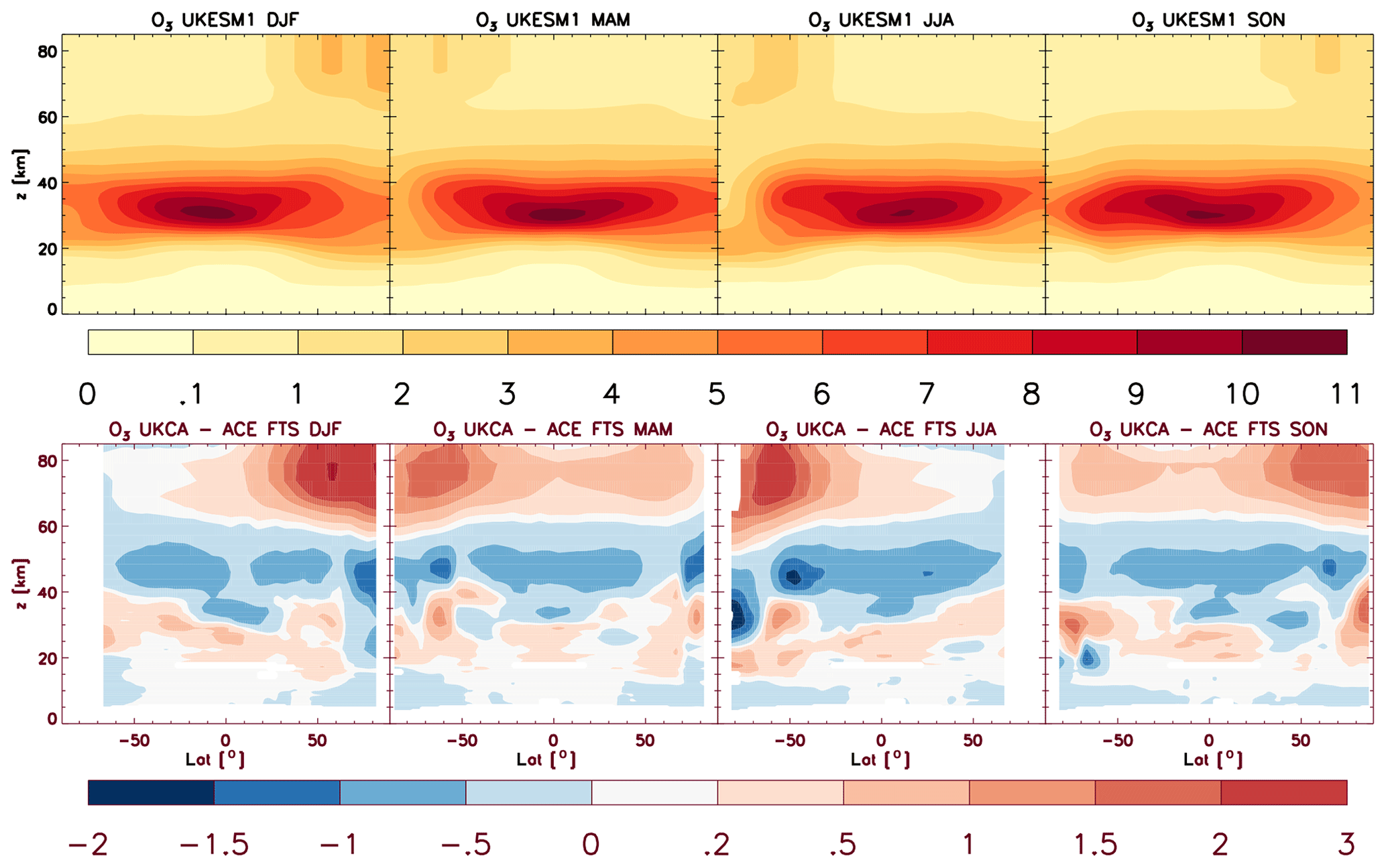
Figure 24 highlights a generally good simulation of stratospheric ozone in UKCA StratTrop. In the lower stratosphere, ozone is mostly overestimated (by around 0.2 to 1 ppm), whereas in the upper stratosphere it is underestimated by similar amounts. Larger underestimations exist in Antarctic winter. In the mesosphere, ozone is generally overestimated.

Taken together, these disagreements indicate some progress with the simulation of odd nitrogen compounds, albeit with substantial remaining problems. HNO₃ is now in better agreement with observations than documented by Morgenstern et al. (2009). However, this appears to be mostly the case because ACE-FTS finds considerably more HNO₃ in the stratosphere than the older Upper Atmosphere Research Satellite (UARS) data used there (Randel et al., 1998). The substantial deficit of NO in the mesosphere is most likely the result of missing model physics: energetic particle precipitation (EPP) is well documented to cause the break-up of nitrogen molecules and the formation of NO_x (for a review see e.g. Sinnhuber et al., 2012), but this process is not represented in UKCA StratTrop. This model deficiency results in a misrepresentation of odd nitrogen descending in the polar vortices towards the ozone layer. This might explain the NO_y deficit in winter–spring over both poles, although further studies are needed to confirm this. This problem is receiving much more attention here than e.g. in the earlier investigation by Morgenstern et al. (2009) because the newer ACE-FTS satellite data offer much better coverage of high latitudes and altitudes than the observational references used by Morgenstern et al. (2009).

Morgenstern et al. (2009) had to artificially reduce water vapour at the tropical tropopause; the reasonable agreement found here is achieved without such an intervention. H₂O loss and CO production are both the result of the photolysis of molecules (CO₂, H₂O) in the mesosphere where the photolysis rate increases sharply with height and may be sensitive to assumptions about the residual ozone column above the model top. In combination, these findings suggest that this residual ozone column (which is a parameter in the photolysis scheme) may be too small or that making this a simple universal constant in the model may be inadequate.

4.7 Analysis of zonal asymmetry of ozone

Stratospheric ozone is often validated against zonal mean satellite data (e.g. see above). As the simulation of ozone improves in models, attention turns to higher-order diagnostics. A recent analysis by Dennison et al. (2017) revealed that zonal asymmetries of the stratospheric polar vortex, in simulations by a model closely related to UKESM1, were strongly underestimated; the vortex was generally too circular and its centre too close to the South Pole, when in reality the southern polar vortex is often distorted and displaced towards the Indian Ocean sector. Dennison et al. found a westward progression of this displacement, which their model failed to reproduce. The climate impacts of ozone depletion are also often thought of in zonal mean terms (e.g. Kang et al., 2011); any effort to attribute regional climate change beyond the zonal mean to ozone depletion might well be impeded by such model behaviour. Hence, here we briefly assess how UKCA StratTrop handles zonal asymmetries of the Antarctic polar vortex. We focus on the CMIP6 coupled historical UKESM1 simulations (Sellar et al., 2019), which use the same version of UKCA StratTrop documented here, rather than the experiments discussed in Sect. 3.

The analysis consists of expanding total column ozone (TCO) in a Fourier series:

$$\begin{array}{}\text{(12)}& \begin{array}{rl}& {\mathrm{O}}_{\mathrm{3}}=\\ & \mathrm{ZMO}\mathrm{3}+A\cos (\mathit{\lambda }+b)+\text{higher-order terms}\text{(ignored here)}.\end{array}\end{array}$$

Here O₃ is monthly mean total-column ozone meridionally averaged over 60 to 70^∘ S, ZMO3 is its zonal mean, $A>=\mathrm{0}$ is the amplitude of the zonal asymmetry, λ is longitude and b is the phase shift; b=0 would correspond to an ozone maximum occurring at the Greenwich Meridian and a minimum occurring at the Date Line. Positive values for b correspond to a westward displacement of these features.

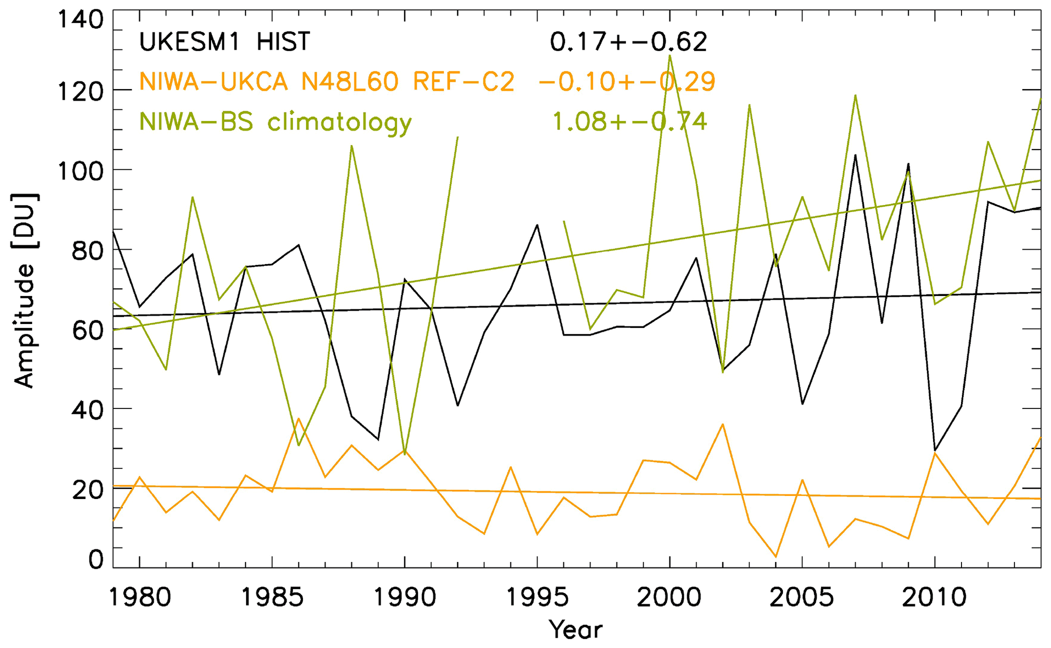
Figure 25 Amplitude A [DU] of the zonal asymmetry in total-column ozone at 60–70^∘ S in October. Green: NIWA–Bodeker Scientific total-column ozone climatology vn 3.4. Orange: the model used by Dennison et al. (2017), NIWA-UKCA. The data represent the average of five CCMI REF-C2 simulations by their model. Black: UKESM1. The data represent the average of two CMIP6 “historical” simulations (Sellar et al., 2019). Straight lines are linear regression fits. The numbers represent mean trends and associated 95 % confidence intervals (DU yr⁻¹).

Figure 25 displays A for October (when the ozone hole is typically deepest). The NIWA–Bodeker Scientific total-column ozone climatology (http://www.bodekerscientific.com/data/total-column-ozone, last access: March 2019; green) indicates that the zonal asymmetry is typically about 40 to 120 DU in size, and on average there is a positive trend, with the ozone asymmetry increasing significantly by nearly 40 DU between 1979 and 2014. UKESM1 (black) reproduces the magnitude and variability of the ozone asymmetry, a big advance over the model used by Dennison et al. (2017) (orange). The difference in the trend is not statistically significant at the 95 % confidence level. For the phase b (Fig. 26) we find that the model produces an ozone peak usually around 60–70^∘ E (i.e. in the Indian Ocean sector), whereas in the NIWA–Bodeker Scientific climatology this maximum occurs further west, on average around 20–30^∘ E. The mean eastward trend simulated by UKESM1 is outside the range of possibilities for the observations (which indicate a westward trend), but the uncertainty intervals overlap.

4.8 Evaluation of transport and long-lived tracer–tracer correlation

Our final aspect of model evaluation focuses on the comparison of the large-scale transport in the modelled middle atmosphere, analysed through a comparison of the modelled age-of-air profiles against the age of air determined using observations of SF₆ made by the MIPAS instrument (Stiller et al., 2008) and through a comparison of observed (ACE-FTS) and modelled tracer–tracer correlations. The model data analysed here are from the FR simulation.

A simple but powerful way to test the representation of stratospheric chemistry in a model is to analyse the correlations between long-lived trace gases (e.g. chap. 6, SPARC 2006). Long-lived tracers are known to exhibit compact correlations with each other (Plumb and Ko, 1992), and comparisons of modelled and observed correlations can test aspects of the model chemistry independent of dynamics. This is particularly useful when comparing complex 3-D climate models such as UKESM1 with observations made by a range of platforms at different spatial resolution and coverage, as well as under different meteorological conditions.

Figure 26 Same as Fig. 25 but for the phase b, in degrees.

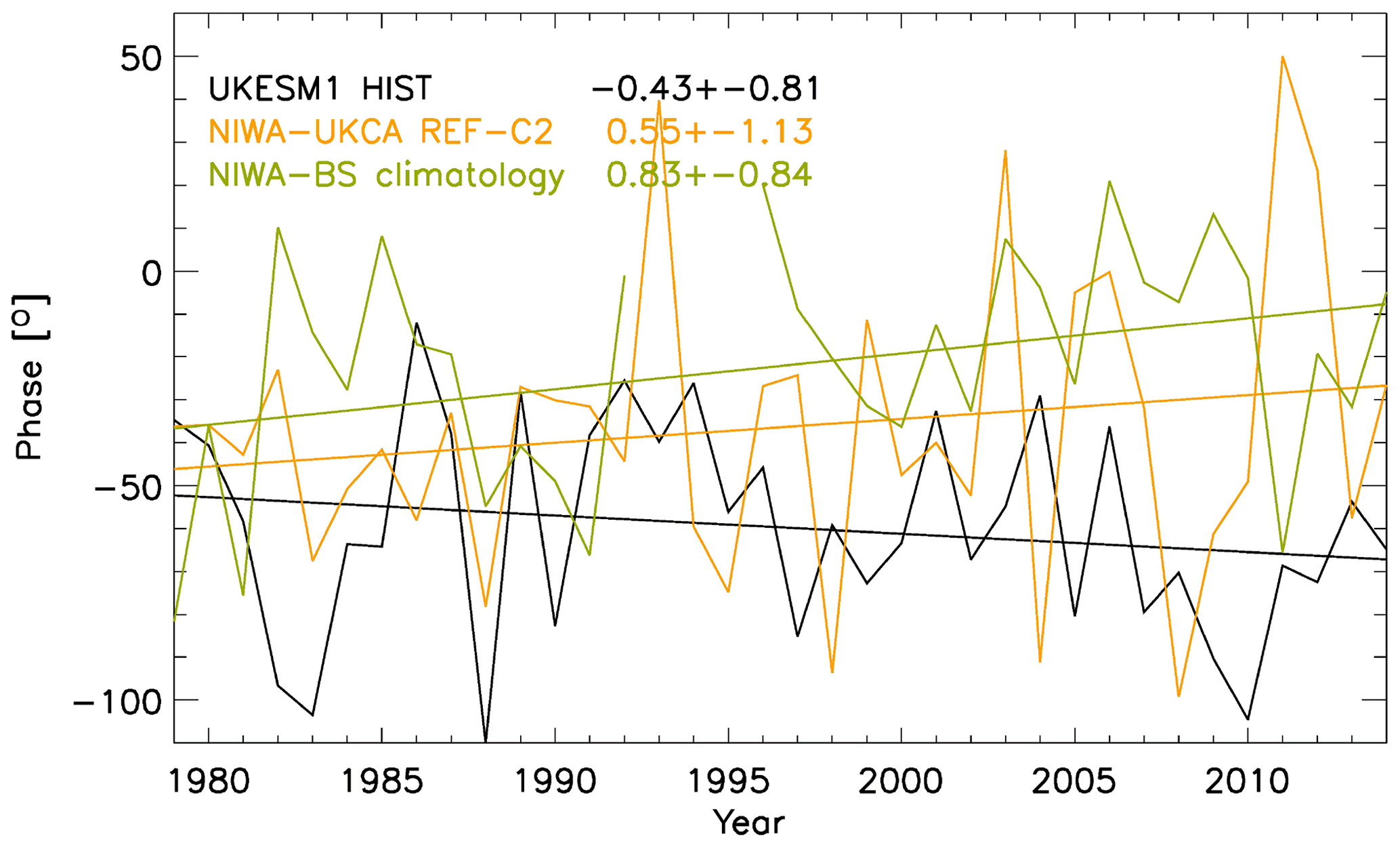
Figure 27 shows the correlations of CH₄ vs. N₂O, CH₄ vs. H₂O and NO_y vs. N₂O from a present-day UKESM1 simulation (2005–2010) as well as from ACE and MIPAS satellite data. The ACE V4 (2004–2018) data were obtained from http://www.ace.uwaterloo.ca/data.php (last access: April 2019), and monthly mean zonal-mean values at 5^∘ latitude bins were created by averaging all profiles with retrieval errors less than 100 %. The Michelson Interferometer for Passive Atmospheric Sounding (MIPAS) V1.4 data used here are an update of those used in the CCMVal-2010 report (SPARC, 2010) (see http://eodg.atm.ox.ac.uk/MIPAS/, last access: April 2019). Co-located profiles of H₂O, CH₄, N₂O, NO₂ and HNO₃ are retrieved simultaneously for both day and night-time profiles and are available for the mission period (2002–2012). MIPAS data were obtained at: ftp://ftp.ceda.ac.uk/neodc/mipas-oxford/data/ (last access: April 2019).

CH₄ and N₂O are two chemically independent but long-lived tracers with significant stratospheric sinks. Accordingly, they are expected to show compact correlations in the stratosphere (Plumb and Ko, 1992). Overall, UKESM1 seems to show very good agreement with the recent satellite-observed relationships, suggesting that the relative loss of CH₄ and N₂O in the stratosphere is well represented. However, the model and the satellite observations differ slightly from the older ER-2 in situ lower stratospheric observations, possibly due to different relative changes in CH₄ and N₂O in recent years. Note also that the model simulation covers the period 2000–2004, while ACE data cover 2004–2018; hence, even after applying the quality flag, ACE CH₄ and N₂O values in the troposphere are larger than model values.

More noticeable model–observation differences are found for the CH₄ : H₂O correlation. These two long-lived tracers are chemically linked in the stratosphere: CH₄ oxidation leads to the production of nearly two molecules of H₂O (with a small yield of H₂). As the maximum observed upper stratosphere H₂O mixing ratio is typically around 7 ppm, and CH₄ is the primary source of stratospheric H₂O, the H₂O vs. CH₄ relationship is expected to be close to ${\mathrm{H}}_{\mathrm{2}}\mathrm{O}+\mathrm{2}\times {\mathrm{CH}}_{\mathrm{4}}=\mathrm{7}$ ppm, which is included in the plots as a reference. The ACE observations show a slightly weaker relationship (${\mathrm{H}}_{\mathrm{2}}\mathrm{O}+\mathrm{1.75}\times {\mathrm{CH}}_{\mathrm{4}}=\mathrm{6.8}$), while MIPAS data show a stronger slope, which is larger than 2 (${\mathrm{H}}_{\mathrm{2}}\mathrm{O}+\mathrm{2.4}\times {\mathrm{CH}}_{\mathrm{4}}=\mathrm{8.0}$). There will be some uncertainty in the satellite data but it is clear that UKESM1 has a significantly different relationship. The upper stratospheric H₂O values are reasonable, but the lower stratosphere seems to be much wetter compared to observations (see Sect. 4.6). For example, near 90 hPa most of the ACE profiles show H₂O values close to 3 ppm, whereas modelled values hardly go below 5 ppm, suggesting that water vapour entry mixing ratios near the tropical tropopause layer are not well constrained in the model. However, in UKESM1 CH₄ oxidation appears to yield only 1 H₂O per CH₄ oxidised, which allows the model to achieve realistic upper stratospheric H₂O values. Further detailed studies are required to verify the cause of this model discrepancy. We have noted that there is a missing H₂O product in the reaction HO₂+MeOO (listed in Table S1). However, we calculate that this reaction only accounts for 2.3 % of the fate of MeOO in the stratosphere (which is dominated by reaction with NO), so it appears unlikely that this is the source of the bias.

Finally, we compare the NO_y vs. N₂O tracers, which are also chemically linked. N₂O is the main source of stratospheric NO_y, with a yield of about 6 % via reaction of O(¹D) (see Eq. 6.2b in SPARC, 2010). ACE NO_y values are calculated simply by adding the observations of HNO₃, NO, NO₂, 2N₂O₅ and ClONO₂. For MIPAS, zonal mean (5^∘ latitude bin) monthly mean profiles were calculated by averaging all the measurements with standard errors less than 100 %. For NO_y : N₂O plots, only night-time profiles are selected (SZA > 95) and NO_y is calculated as ${\mathrm{HNO}}_{\mathrm{3}}+{\mathrm{NO}}_{\mathrm{2}}+\mathrm{2}{\mathrm{N}}_{\mathrm{2}}{\mathrm{O}}_{\mathrm{5}}+{\mathrm{ClONO}}_{\mathrm{2}}$. For large values of N₂O, the UKESM1 correlation is less compact than the observations, although the modelled slope indicates a realistic 6.7 % yield of NO_y. The model also produces a reasonable peak NO_y mixing ratio of around 17 ppb, although this is slightly smaller than observations, in particular from ACE. The model also tends to simulate larger occurrences of low NO_y values for a given N₂O, which may be an indication of strong polar denitrification.

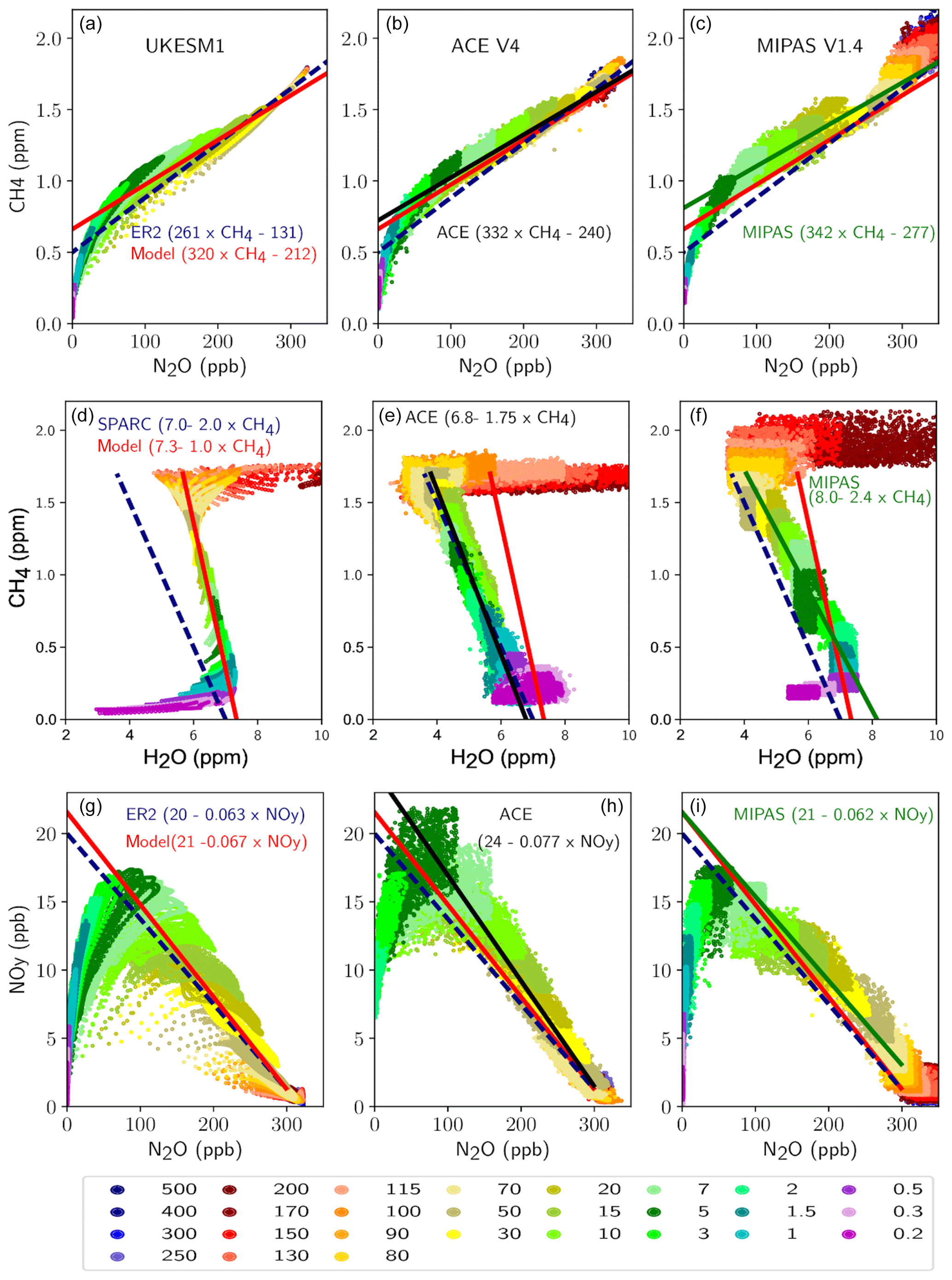
Figure 27 Correlations between selected long-lived chemical species (monthly mean zonal-mean values for 60^∘ S–60^∘ N) from FR UKESM1 (a, d, g), ACE V4 data (b, e, h) and MIPAS data (c, f, i). The coloured legend shows the corresponding pressure level (hPa) of the data points. The linear regression fits to the model, ACE and MIPAS data are shown in the respective panels along with the equations of the lines. The MIPAS data are the same as those used in Figs. 6.12, 6.13 and 6.14 in the CCMVal-2 report (SPARC, 2010). ACE NO_y values are calculated as ${\mathrm{NO}}_y=\mathrm{NO}+{\mathrm{NO}}_{\mathrm{2}}+{\mathrm{HNO}}_{\mathrm{3}}+\mathrm{2}{\mathrm{N}}_{\mathrm{2}}{\mathrm{O}}_{\mathrm{5}}+{\mathrm{ClONO}}_{\mathrm{2}}$. (a–c) CH₄ vs. N₂O. The linear fit is calculated for N₂O values ranging from 100 to 300 ppb. The dashed line shows the estimated fit from ER-2 data (N₂O (ppb) $=\mathrm{261.8}\times {\mathrm{CH}}_{\mathrm{4}}$ (ppm) −131; see Kawa et al., 1993). (d–f) CH₄ vs. H₂O. The linear fit is calculated for CH₄ values ranging from 0.5 to 1.5 ppm. The dashed line represents ${\mathrm{H}}_{\mathrm{2}}\mathrm{O}+\mathrm{2}{\mathrm{CH}}_{\mathrm{4}}=\mathrm{7}$ ppm. (g–i) NO_y vs. N₂O. The linear fit is calculated for N₂O values ranging from 100 to 300 ppb, and the dashed line shows the equation NO_y (ppb) $=\mathrm{20.0}-\mathrm{0.0625}\times {\mathrm{N}}_{\mathrm{2}}\mathrm{O}$ (ppb) based on mid-latitude balloon profiles and ER-2 data (see Kondo et al., 1996).

Figure 28 compares data from the FR simulation and observations. The FR run is shown here as this allows for a more robust comparison of the model data where it is not constrained by the reanalysis meteorology. Figure 28 shows the modelled multi-annual mean age-of-air profile in the stratosphere against observations of SF₆ from 2002 to 2010 used to calculate the age of air from the MIPAS instrument (Stiller et al., 2008). The model includes a diagnostic to quantify the age of air. This is effectively a “species” in the model that is emitted at the model surface continually and undergoes full tracer advection and diffusion. Whilst below the modelled tropopause (based on a merger of the 380 K and 2 PVU surfaces) the tracer is set to have an age of zero, above the tropopause the tracer has its age increased every model time step that it stays above the tropopause.

Figure 28 Comparison of multi-annual mean FR modelled (red) age of air with values derived from MIPAS observations of SF₆ (black) (Stiller et al., 2008). (a) Tropical profile. (b) NH mid-latitude profile. (c) Mid-latitude tropics profile. (d) Mean age at 23 km (∼50 hPa).

Figure 28a shows the modelled mean tropical (±10^∘) age profile as a function of altitude and that there is very good agreement between the model and the values derived from MIPAS observations, with an increase in the age of air as both profiles increase in altitude and a maximum age of around 5 years. The modelled Northern Hemisphere mid-latitude (35–45^∘ N) age profile (panel b) agrees very well with the observations from 16 to about 24 km, but the model tends to simulate an age of air which is younger than the observations above 24 km (up to a year difference younger). Panel (c) shows the difference between the mid-latitude and tropical profiles and further emphasises the good agreement of the model with the observations below 23 km but divergence above this altitude. However, the zonal cross section at 23 km (∼ 50 hPa) (panel d) shows that the model generally falls within the observational uncertainty (1 standard deviation of the multi-annual observations) at all latitudes.

5 Discussion and conclusions

In this paper we have documented the species and reactions that make up the UKCA StratTrop mechanism for the first time and performed an evaluation of the model output for the recent past. UKCA is the module for simulating chemical and aerosol processes in the UKESM1 Earth system model (Sellar et al., 2019), and UKCA StratTrop enables a holistic representation of gas-phase chemistry in the troposphere and stratosphere, which is important for understanding short-lived climate forcers.

Our focus here has been to document the performance of the chemical fields simulated by UKCA StratTrop as implemented in UKESM1; the aerosol schemes, processes and performance are discussed in detail in Mulchay et al. (2020). Further studies are planned which will assess the role of composition–climate Earth system couplings in the UKESM1 framework. Hence, we present simulations which have enabled a more focused assessment of key performance indicators of the UKCA StratTrop scheme. We have analysed data from two model runs; the first was a free-running (FR) simulation wherein the meteorology was allowed to evolve independently based on the influence of the prescribed forcing agents (sea surface temperatures, greenhouse gases and sea ice), and the second was a nudged (ND) simulation wherein the meteorology was relaxed toward the ERA-Interim reanalysis.

In general, and focusing on the gas phase as we have here, we find that the performance of UKCA StratTrop in UKESM1 is in line with the range of models that are applied to simulating the coupled chemistry–climate system (Young et al., 2013, 2018).

Our key performance indicators have included the following.

• An assessment of the magnitude and spatial distribution of lightning NO_x: we note here that whilst the model simulates a global annual total lightning NO_x emissions magnitude that is in the middle of the range quoted in the literature based on observational constraints (∼ 6 Tg yr⁻¹), and the spatial distribution in lightning flash frequency matches well with observations from satellites, the variability in lightning flash frequency is not in good agreement with the observations (Fig. 2). The UKESM1 model predicts too much lightning activity in the tropics at the expense of the extratropics, something which could be resolved by moving to an ice-flux-based scheme (Finney et al., 2018). Moreover, the vertical profile of lightning NO_x may have a significant impact on modelled O₃. Hakim et al. (2019) have shown that across India the vertical profile in simulated lightning NO_x is very model-dependent. We suggest that further work be performed to better understand the impacts of both the spatial distribution of lightning NO_x and the impacts of lightning NO_x on the tropospheric column biases in O₃ in the model.

• Surface ozone correlations and mean bias against TOAR observations: TOAR (Schultz et al., 2018) provides the chemistry modelling community with an unprecedented dataset to evaluate surface O₃. In our analysis of the FR and ND runs presented here, we show that the annual mean bias is very low, but this hides biases in summer and wintertime (Young et al., 2018). However, we suggest that further work be performed to understand the cause of the low and high biases in surface O₃, especially with regards to how these may impact studies that use UKESM1 surface O₃ in health assessment studies.

• The tropospheric oxidising capacity: a key component to determine the lifetime of emitted reactive gases in the troposphere is the oxidising capacity. Whilst this has to be inferred from observations (i.e. through the inferred lifetime of methane) it is an important metric to evaluate the model against. In this study we found that the methane lifetime in the troposphere with respect to OH was 8.5 years, which is within the ACCMIP multi-model range but slightly low compared to observational analyses (Naik et al., 2013). When compared against other model estimates of the zonal mean distribution of OH, UKESM1 performs well in 10 out of 12 regions analysed, with a significant high bias in the tropical boundary layer. This is a region where the majority of methane oxidation takes place and may explain the slightly low modelled methane lifetime. With the recent development of aircraft OH datasets appropriate for global model evaluation (Prather et al., 2017) we intend to extend this analysis further and interrogate the model with these data to confirm if the bias is indeed large compared with direct observations.

• Tropospheric columns of reactive gases (CO, NO₂ and O₃): the analysis of the model ND runs highlighted some success and failure in the model's representation of tropospheric columns of CO, NO₂ and O₃. The best performance was found for O₃ (Figs. 14–15), although we note that there is a significant positive bias in the tropics (which has been shown to have an effect on modelled tropospheric photolysis rates; Hall et al., 2018). In part we believe this bias is connected with the vertical profile and magnitude of lightning NO_x, and further work will focus specifically on this area. The modelled tropospheric column of CO shows significant negative biases in the Northern Hemisphere (Fig. 16). In part this is believed to relate to biases in the representation of higher hydrocarbons that could contribute significantly to secondary CO production (Grant et al., 2010), but high OH could also be a contributing factor. The performance of modelled NO₂ tropospheric columns was found to be generally acceptable in northern mid-latitudes (Fig. 19), but there are large biases in regions of high emissions (such as the North China Plain; Fig. 18). One hypothesis is that the model simulates too little OH in the regions of high NO₂ emissions owing to a lack of reactive VOC emissions and titration of O₃, which extends the lifetime of NO₂ in these regions. Further studies are required to evaluate the modelled NO₂ lifetime and its response to changes in emissions of NO_x.

• Biases in stratospheric composition: by examining selected climatologies of observations from satellites (Figs. 20–24) we have been able to show here that the simulation of stratospheric composition has improved significantly in StratTrop compared with the older “stratosphere”-focused scheme of MO09. In part this is largely due to improvements in the dynamical model (MetUM) and reductions in biases in modelled water vapour (Hardiman et al., 2015). Key questions remain about the fidelity of the upper stratospheric–mesospheric photolysis rates and the upper boundary conditions. Given the generally poorer performance of NO and NO_y it would be useful to investigate the implementation of parameterised EPP to see if this ameliorates the problems. Further work is also required to understand the cause of the disagreement between the CH₄ : H₂O correlation in the stratosphere, which suggests that too little H₂O is produced from methane oxidation in the model.

• Middle atmosphere age of air: the modelled middle atmosphere circulation has been evaluated against the age of air derived from observations of SF₆ and through the use of tracer–tracer correlations. These tracer–tracer correlations further motivate the need for a more detailed investigation of modelled stratospheric NO_y and its budget (production and loss). The comparison of the age of air in the model generally looks acceptable in the middle stratosphere but tends to deviate at higher altitudes. In part there is more uncertainty in observations at higher altitudes (owing to loss processes of SF₆), but further studies are required to understand if these biases are dependent on the resolution of the model. To understand this, a high-top (> 120 km) version of the model is in preparation, as are simulations of UKESM1 at much higher horizontal resolution (∼ 25 km).

In summary, UKCA StratTrop represents a substantial step forward compared to previous versions of UKCA. We have shown here that it is well suited to the challenges of representing interactions in a coupled Earth system model (key for CMIP6 and beyond), and we have identified key areas and components for future development that will further improve the model.