the Creative Commons Attribution 4.0 License.
the Creative Commons Attribution 4.0 License.
 | 10 Mar 2020
Development of Korean Air Quality Prediction System version 1 (KAQPS v1) with focuses on practical issues
Kyunghwa Lee
Jinhyeok Yu
Sojin Lee
Mieun Park
Hun Hong
Soon Young Park
Myungje Choi
Jhoon Kim
Younha Kim
Jung-Hun Woo
Sang-Woo Kim
Chul H. Song
For the purpose of providing reliable and robust air quality predictions, an air quality prediction system was developed for the main air quality criteria species in South Korea (PM10, PM2.5, CO, O3 and SO2). The main caveat of the system is to prepare the initial conditions (ICs) of the Community Multiscale Air Quality (CMAQ) model simulations using observations from the Geostationary Ocean Color Imager (GOCI) and ground-based monitoring networks in northeast Asia. The performance of the air quality prediction system was evaluated during the Korea-United States Air Quality Study (KORUS-AQ) campaign period (1 May–12 June 2016). Data assimilation (DA) of optimal interpolation (OI) with Kalman filter was used in this study. One major advantage of the system is that it can predict not only particulate matter (PM) concentrations but also PM chemical composition including five main constituents: sulfate (), nitrate (), ammonium (), organic aerosols (OAs) and elemental carbon (EC). In addition, it is also capable of predicting the concentrations of gaseous pollutants (CO, O3 and SO2). In this sense, this new air quality prediction system is comprehensive. The results with the ICs (DA RUN) were compared with those of the CMAQ simulations without ICs (BASE RUN). For almost all of the species, the application of ICs led to improved performance in terms of correlation, errors and biases over the entire campaign period. The DA RUN agreed reasonably well with the observations for PM10 (index of agreement IOA =0.60; mean bias MB ) and PM2.5 (IOA =0.71; MB ) as compared to the BASE RUN for PM10 (IOA =0.51; MB ) and PM2.5 (IOA =0.67; MB ). A significant improvement was also found with the DA RUN in terms of bias. For example, for CO, the MB of −0.27 (BASE RUN) was greatly enhanced to −0.036 (DA RUN). In the cases of O3 and SO2, the DA RUN also showed better performance than the BASE RUN. Further, several more practical issues frequently encountered in the air quality prediction system were also discussed. In order to attain more accurate ozone predictions, the DA of NO2 mixing ratios should be implemented with careful consideration of the measurement artifacts (i.e., inclusion of alkyl nitrates, HNO3 and peroxyacetyl nitrates – PANs – in the ground-observed NO2 mixing ratios). It was also discussed that, in order to ensure accurate nocturnal predictions of the concentrations of the ambient species, accurate predictions of the mixing layer heights (MLHs) should be achieved from the meteorological modeling. Several advantages of the current air quality prediction system, such as its non-static free-parameter scheme, dust episode prediction and possible multiple implementations of DA prior to actual predictions, were also discussed. These configurations are all possible because the current DA system is not computationally expensive. In the ongoing and future works, more advanced DA techniques such as the 3D variational (3DVAR) method and ensemble Kalman filter (EnK) are being tested and will be introduced to the Korean air quality prediction system (KAQPS).
- Article
(2961 KB) - Full-text XML
- BibTeX
- EndNote


Air quality has long been considered an important issue in climate change, visibility and public health, and it is strongly dependent upon meteorological conditions, emissions and the transport of air pollutants. Air pollutants typically consist of atmospheric particles and gases such as particulate matter (PM), carbon monoxide (CO), ozone (O3), nitrogen dioxide (NO2) and sulfur dioxide (SO2). These aerosols and gases play important roles in anthropogenic climate forcing, both directly (Bellouin et al., 2005; Carmichael et al., 2009; IPCC, 2013; Scott et al., 2014) and indirectly (Breon et al., 2002; IPCC, 2013; Penner et al., 2004; Scott et al., 2014) influencing the global radiation budget. Among the various air pollutants, PM and surface O3 are the most notorious health threats, as has been stated by several previous studies (Carmichael et al., 2009; Dehghani et al., 2017; Khaniabadi et al., 2017).
With the stated importance of atmospheric aerosols and gases, considerable research efforts have been made to monitor and quantify their amounts in the atmosphere through satellite-, airborne- and ground-based observations as well as chemistry-transport model (CTM) simulations. In South Korea, the Korean Ministry of the Environment (KMoE) provides real-time chemical concentrations as measured by ground-based observations for six air quality criteria air pollutants (PM10, PM2.5, O3, CO, SO2 and NO2) at the Air Korea website (https://www.airkorea.or.kr, last access: 8 March 2020). PM10 or (PM2.5) refers to the atmospheric particulate matter that has an aerodynamic diameter less than 10 (or 2.5) µm. In addition, the National Institute of Environmental Research (NIER) of South Korea provides air quality predictions using multiple CTM simulations. Air quality predictions are another crucial element for protecting public health through the forecasting of high air pollution episodes in advance and alerting citizens about these high episodes. In this context, reliable and robust air quality forecasts are necessary to avoid any confusion caused by poor predictions given by CTM simulations.
Although there are various datasets representing air quality, limitations remain in the observations and model outputs. Specifically, observation data are, in general, known to be more accurate than model outputs, but they have spatial and temporal limitations. These limitations will be overcome by improving spatial and temporal coverage via future geostationary satellite instruments such as the Geostationary Environment Monitoring Spectrometer (GEMS) over Asia, the Tropospheric Emissions: Monitoring of Pollution (TEMPO) over North America and the Sentinel-4 over Europe. In addition, the TROPOspheric Monitoring Instrument (TROPOMI) on board the Copernicus Sentinel-5 Precursor satellite was successfully launched into low earth orbit (LEO) on 13 October 2017 and is providing information on the chemical composition in the atmosphere with a higher spatial resolution of 3.5 km×7 km.
Unlike observational data, models can provide meteorological and chemical information without any spatial and temporal data discontinuity, but they do have an issue of inaccuracy. The major causes of uncertainty in the results of CTM simulations are introduced from imperfect emissions, meteorological fields, initial conditions (ICs), and physical and chemical parameterizations in the models (Carmichael et al., 2008). In order to minimize the limitations and maximize the advantages of observation data and model outputs, there have been numerous attempts to provide accurate and spatially as well as temporally continuous information on chemical composition in the atmosphere by integrating observation data with model outputs via data assimilation (DA) techniques.
Although the Korean numerical weather prediction (NWP) carried out by the Korea Meteorological Administration (KMA) employs various DA techniques, almost no previous efforts have been made to develop an air quality prediction system with DA in South Korea. Therefore, in the present study, the air quality prediction system named as Korean Air Quality Prediction System version 1 (KAQPS v1) was developed by preparing ICs via DA for the Community Multiscale Air Quality (CMAQ) model (Byun and Schere, 2006; Byun and Ching, 1999) using satellite- and ground-based observations for particulate matter (PM) and atmospheric gases such as CO, O3 and SO2. The performances of the system were then demonstrated during the period of the Korea-United States Air Quality Study (KORUS-AQ) campaign (1 May–12 June 2016) in South Korea.
In this study, the optimal interpolation (OI) method with the Kalman filter was applied in order to develop the air quality prediction system, since this method is still useful and viable in terms of computational cost and performance. The performance of the method is almost comparable to that of the 3D variational (3DVAR) method, as shown in Tang et al. (2017). More complex and advanced DA techniques are currently being and will continue to be applied to current air quality prediction systems. These works are now in progress.
In addition, this paper also discusses several practical issues frequently encountered in the air quality predictions such as (i) DA of NO2 mixing ratios for accurate ozone prediction with a careful consideration of measurement artifacts; (ii) the issue of the nocturnal mixing layer height (MLH) for nocturnal predictions; (iii) predictions of dust episodes; (iv) the use of non-static free parameters; and (v) the influences of multiple implementations of the DA before the actual predictions.
The details of the datasets and methodology used in this study are described in Sect. 2. The results of the developed air quality prediction system are discussed in Sect. 3, and then a summary and conclusions are given in Sect. 4.
The air quality prediction system was developed using the CMAQ model along with meteorological inputs provided by the Weather Research and Forecasting (WRF) model (Skamarock et al., 2008). The ICs for the CMAQ model simulations were prepared via the DA method using satellite-retrieved and ground-based observations. The performances of the developed prediction system were evaluated using ground in situ data. The models, data and DA technique are described in detail in the following sections.
2.1 Meteorological and chemistry-transport modeling
2.1.1 WRF model simulations
The WRF model has been developed for providing mesoscale numerical weather prediction (NWP). It has also been used to provide meteorological input fields for CTM simulations (Appel et al., 2010; Chemel et al., 2010; Foley et al., 2010; Lee et al., 2016; Park et al., 2014). In this study, WRF v3.8.1 with the Advanced Research WRF (ARW) dynamical core was applied to prepare the meteorological inputs for the CMAQ model simulations. Dynamical and physical configurations for the WRF model simulations were selected as follows: the Yonsei University (YSU) scheme for planetary boundary layer (Hong et al., 2006); the WRF single-moment 6-class (WSM6) scheme for the microphysics (Hong and Lim, 2006); the Grell–Freitas ensemble scheme for cumulus parameterization (Grell and Freitas, 2014); the Noah-MP land surface model (Niu et al., 2011; Yang et al., 2011); the Rapid Radiative Transfer Model for Global Circulation Models (RRTMG) for shortwave/longwave options (Iacono et al., 2008); and the revised MM5 scheme for surface layer options (Jimenez et al., 2012). The National Centers for Environmental Prediction (NCEP) Final (FNL) Operational Global Analysis data on grids were chosen for the ICs and boundary conditions (BCs) for the WRF simulations. In order to minimize meteorological field errors for the applications of ICs and BCs to the WRF simulations, the objective analysis (OBSGRID) nudging was conducted using the NCEP Automated Data Processing (ADP) Global Upper Air Observations/Surface Observational weather data via the Cressman's (1959) successive correction method. The adjusted meteorological variables were temperature, geopotential height, relative humidity and zonal/meridional winds.
The model domain for the WRF simulations covers northeast Asia with a horizontal resolution of 15 km×15 km, having a total of 223 latitudinal and 292 longitudinal grid cells. The size of the WRF domain is slightly larger than that of the CMAQ domain, as shown in Fig. 1. The meteorological data have 27 vertical layers from the surface (1000 hPa) to 50 hPa. The WRF meteorological fields (e.g., temperature, pressure, wind, humidity, and clouds) were then transformed into the CMAQ-ready format via the Meteorology-Chemistry Interface Processor (MCIP; Otte and Pleim, 2010) v4.3, which is a software to serve for transforming horizontal and vertical coordinates while trying to maintain dynamic consistency between WRF and CMAQ model simulations.
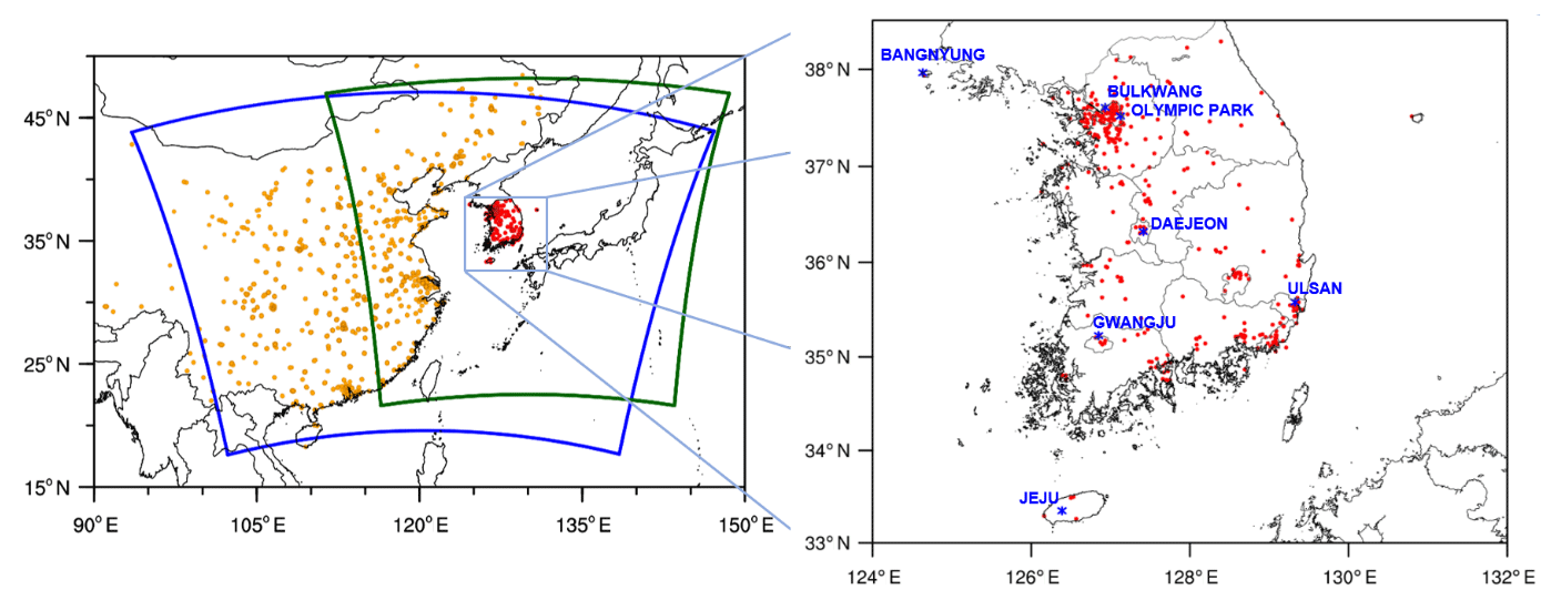
Figure 1Domains of GOCI sensor (dark green line) and CMAQ model simulations (blue line). Red-colored dots denote the locations of Air Korea sites in South Korea. Orange-colored dots represent the locations of ground-based observation stations in China. Blue stars show the locations of seven supersites in South Korea. During the KORUS-AQ campaign, observation data were obtained from 1514 stations in China as well as 264 Air Korea and seven supersite stations in South Korea. NCL (2019) was used to draw this figure.
2.1.2 CMAQ model simulations
The CMAQ v5.1 model was used to estimate the concentrations of the atmospheric chemical species over the domain, as shown in Fig. 1. The CMAQ domain has 204 latitudinal and 273 longitudinal grid cells in total and also has a 15 km×15 km horizontal resolution and 27 vertical layers. The CMAQv5.1 model was configured to use. Chemical and physical configurations for the CMAQ model simulations were selected as follows: SAPRC07tc for the gas-phase chemical mechanism (Hutzell et al., 2012); AERO6 for aerosol thermodynamics (Appel et al., 2013); Euler Backward Iterative (EBI) chemistry solver (Hertel et al., 1993), which is a numerically optimized photochemistry mechanism solver; M3DRY for dry deposition velocity (Pleim and Xiu, 2003; Xiu and Pleim, 2001); global mass-conserving scheme (Yamartino and WRF) for horizontal and vertical advection (Colella and Woodward, 1984); MULTISCALE (Louis, 1979), which is a simple first-order eddy diffusion scheme for horizontal diffusion; and the Asymmetric Convective Model, version 2 (ACM2; Pleim, 2007a, b), for vertical diffusion.
For anthropogenic emissions, KORUS v1.0 emissions (Woo et al., 2012) were used. The emissions cover almost all of Asia and are based on three emission inventories: the Comprehensive Regional Emissions inventory for Atmospheric Transport Experiment (CREATE) for East Asia excluding Japan; the Model Inter-Comparison Study for Asia (MICS-Asia) for Japan; and the Studies of Emissions and Atmospheric Composition, Clouds and Climate Coupling by Regional Surveys (SEAC4RS) for South and Southeast Asia.
Biogenic emissions were prepared by running the Model of Emissions of Gases and Aerosols from Nature (MEGAN v2.1; Guenther et al., 2006, 2012) with a grid size identical to that of the CMAQ model simulations. For the MEGAN simulations, the MODIS land cover data (Friedl et al., 2010) and improved leaf area index (LAI) based on MODIS datasets (Yuan et al., 2011) were utilized. Pyrogenic emissions were obtained from the Fire Inventory from NCAR (FINN; Wiedinmyer et al., 2006, 2011). The lateral BCs for the CMAQ model simulations were prepared using the global model results of the Model for Ozone and Related chemical Tracers, version 4 (MOZART-4; Emmons et al., 2010) at every 6 h. The mapping and regridding of the MOZART-4 data were conducted by matching the CMAQ grid information.
2.2 Observation data
2.2.1 Satellite-based observations
A Korean geostationary satellite of Communication, Ocean and Meteorological Satellite (COMS) was launched on 26 June in 2010 over the Korean Peninsula. The COMS is a geostationary orbit satellite, and it is stationed at an altitude of approximately 36 000 km at a latitude of 36∘ N and a longitude of 128.2∘ E, with a horizontal coverage of 2500 km×2500 km (refer to Fig. 1). Among the three payloads of the COMS, Geostationary Ocean Color Image (GOCI) is the first multichannel ocean color sensor with visible and near-infrared channels. The GOCI instrument provides hourly spectral images with a spatial resolution of 500 m×500 m from 00:30 to 07:30 coordinated universal time (UTC) for eight spectral (six visible and two near-infrared) channels at 412, 443, 490, 555, 660, 680, 745 and 865 nm.
The Yonsei aerosol retrieval (YAER) algorithm for the GOCI sensor was initially developed by Lee et al. (2010) to retrieve the aerosol optical properties (AOPs) over ocean areas and was then improved by expanding to consider nonspherical aerosol optical properties (Lee et al., 2012). Choi et al. (2016) further extended the algorithm for application to land surfaces, and the algorithm was referred to as the GOCI YAER version 1 algorithm. With the GOCI YAER algorithm, hourly aerosol optical depths (AODs) at 550 nm were produced over East Asia. Choi et al. (2016) compared the retrieved GOCI AODs with other satellite-retrieved and ground-based observations and found several errors in the cloud masking and surface reflectances. These errors were corrected in the recently updated second version of the GOCI YAER algorithm (Choi et al., 2018), which used the updated cloud masking and more accurate surface reflectances. In this study, the most recent GOCI AOD products from the GOCI YAER version 2 algorithm were used.
2.2.2 Ground-based observations
In addition to the satellite data, ground-based observations in South Korea and China were also collected for use in the air quality prediction system for PM and gas-phase pollutants. The orange, red and blue dots in Fig. 1 represent the ground-based observation sites in China, Air Korea and supersite stations in South Korea, respectively. These observations provide real-time concentrations of air quality criteria species such as PM10, PM2.5, CO, O3, SO2 and NO2.
Throughout the period of the KORUS-AQ campaign, ground-based observation data were obtained from 1514 stations in China, 264 Air Korea stations and seven supersite stations in South Korea. In this study, 80 % of the ground-based observations in China and Air Korea stations in South Korea were randomly selected for use in the prediction system. The other 20 % of the data and supersite observations were used to evaluate the performances of the developed air quality prediction system.
In addition, AErosol RObotic NETwork (AERONET) AODs were used to conduct an independent evaluation of the air quality prediction system. AERONET is a federated global ground-based sun photometer network (Holben et al., 1998). Cloud-screened and quality-assured level 2.0 AODs for the AERONET were used in this study.
2.3 Air quality prediction system
In the present study, the air quality prediction system was developed by adjusting the ICs for the CMAQ model simulations based on DA with satellite-retrieved and ground-measured observations. Two parallel WRF-CMAQ model runs were conducted. The first experiment that involved adjusting ICs via DA is referred to as DA RUN (see Fig. 2). In order to evaluate the prediction system, a second experiment, in which the ICs were originated from the previous CMAQ model simulations without assimilations, was also conducted. This CMAQ run is referred to as BASE RUN.
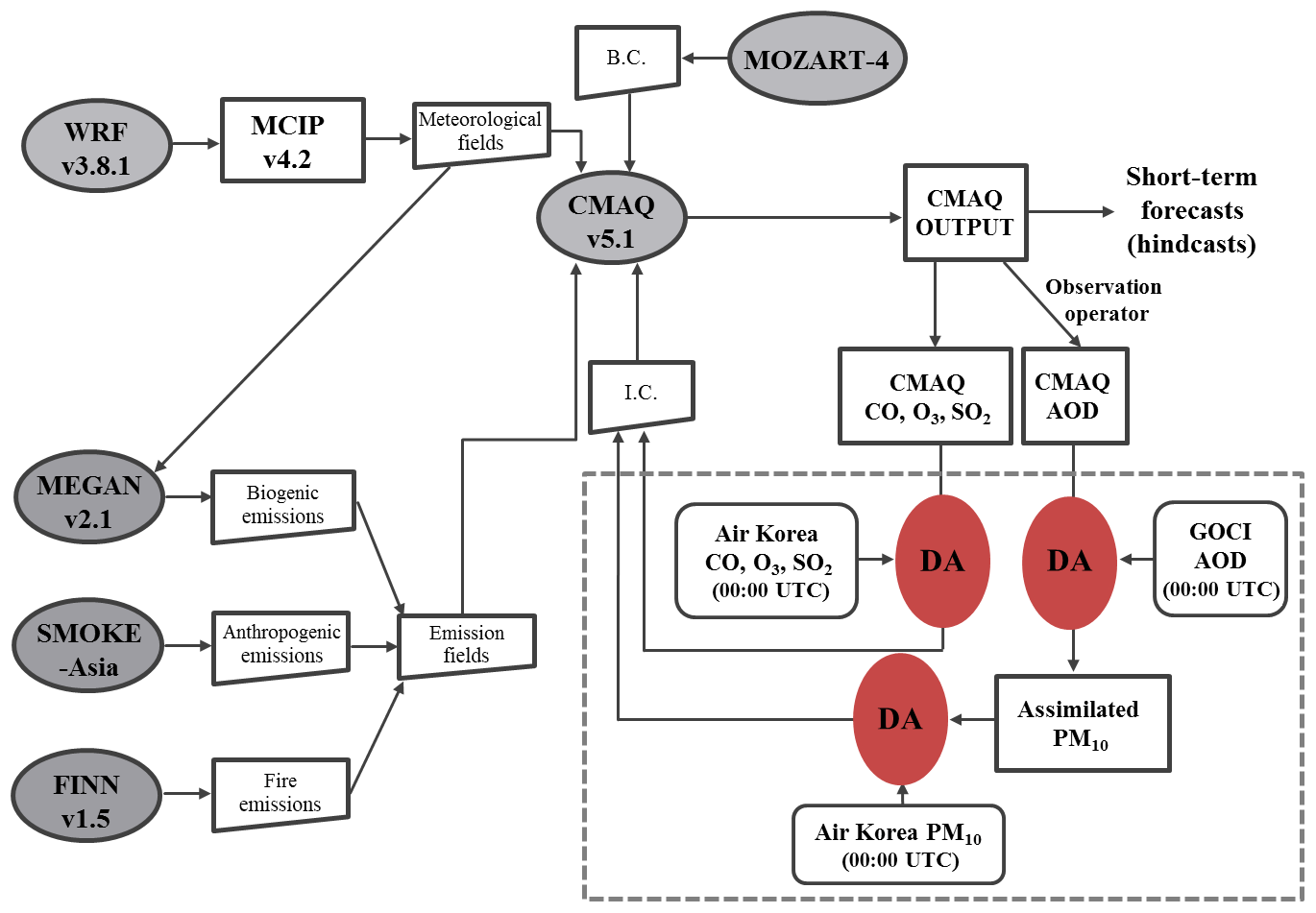
Figure 2Schematic diagram of the Korean air quality prediction system developed in this study. The initial conditions (ICs) of the CMAQ model simulations are prepared by assimilating CMAQ outputs with satellite-retrieved and ground-measured observations. The data process for preparing the ICs is shown in the box with dashed gray lines.
2.3.1 AOD calculations
CMAQ AODs are calculated by integrating the aerosol extinction coefficient (σext) using the following equation:
where z represents the vertical height; σext is defined as the sum of the absorption coefficient (σabs) and the scattering coefficient (σsca); and σabs and σsca can be estimated by Eqs. (3) and (4), respectively, as shown below.
where i and j denote the particulate species and size bin (or particle mode), respectively; ωij(λ) is the single scattering albedo; βij(λ) is the mass extinction efficiency (MEE) of particulate species i for the size bin or particle mode j; [C]ij is the concentration of particulate species including , black carbon, organic aerosols (OA), mineral dust and sea-salt aerosols; RH is the relative humidity; fij(RH) is the hygroscopic factor; and the single scattering albedo (ω) implies to the fraction (portion) of scattering in the total extinction.
Using Eqs. (2)–(4), AODs were calculated from the aerosol composition and RH. There have been intensive tests using different β and f(RH) values in the following three previous studies: (1) Chin et al.'s (2002) study with the Goddard Chemistry Aerosol Radiation and Transport (GOCART) model; (2) Martin et al.'s (2003) study with the GEOS-Chem model; and (3) Malm and Hand's (2007) study with the CMAQ model. Lee et al. (2016) tested these methods and then found that Chin et al.'s (2002) method reproduced the best results in estimating AODs at 550 nm over East Asia. On the basis of Lee et al.'s (2016) work, σext was estimated with the β and f(RH) values suggested by Chin et al. (2002). After that, σext was integrated with respect to altitude, in order to calculate the AODs. The calculated AODs were used in the air quality prediction system in order to prepare the ICs for the PM predictions.
2.3.2 Data assimilation (DA)
The ground-based observations, together with GOCI-derived AODs, were used to prepare the ICs for the air quality predictions with the CMAQ model simulations. In order to achieve this, the following steps were taken: (i) the CMAQ-calculated concentrations of CO, O3 and SO2 were combined with the concentrations of CO, O3 and SO2 obtained from ground-based observations in South Korea (Air Korea) and China; (ii) the CMAQ-calculated AODs were assimilated with the GOCI AODs; (iii) the assimilated AODs were converted into PM10; (iv) the converted PM10 was again assimilated at the surface in South Korea and China; and (v) after the DA at the surface, the ratios of the assimilated species concentrations to the original CMAQ-simulated concentrations were applied so as to the adjust vertical profiles of the chemical species above the surface. In the air quality prediction system, the DA cycle is 24 h, and the assimilation takes place every day at 00:00 UTC (refer to Fig. 3).
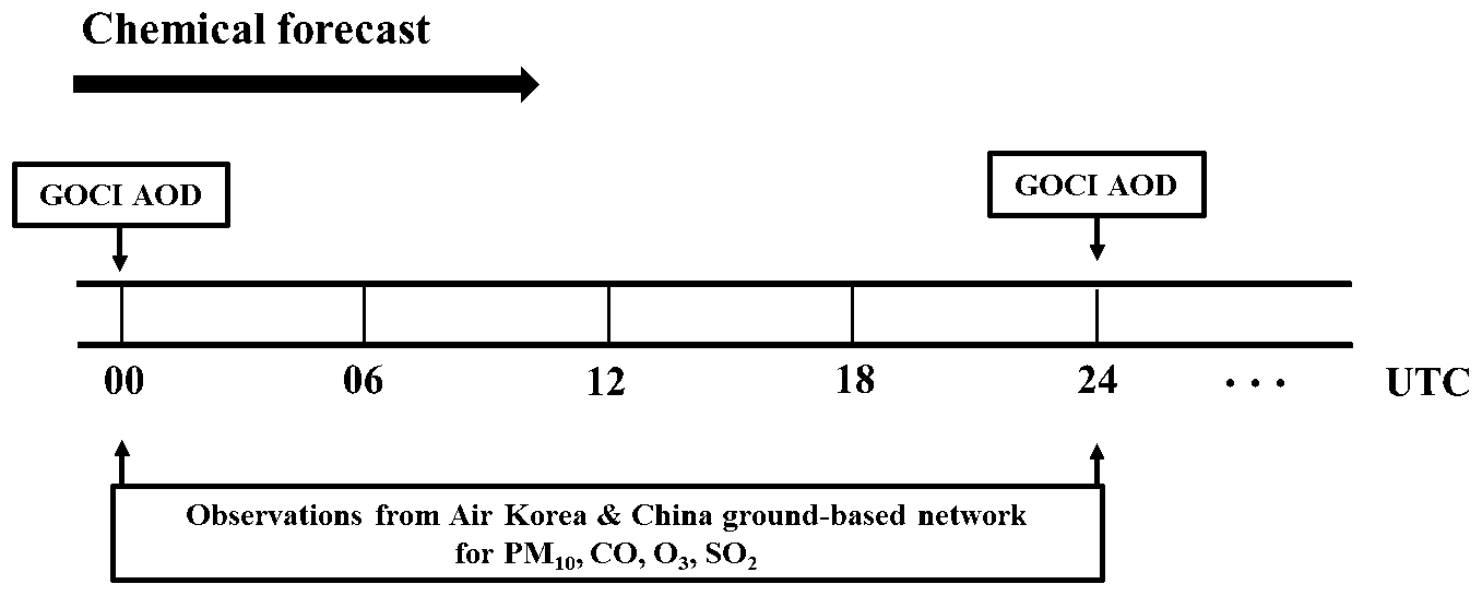
Figure 3Schematic diagram of the Korean air quality prediction system for particulate matter (PM) and gas-phase pollutants. The data assimilation (DA) cycle is 24 h for both PM and gas-phase pollutants such as CO, O3 and SO2. The DA of NO2 is excluded in the current study, the reason for which is discussed in the text.
The optimal interpolation (OI) method with the Kalman filter was chosen in the air quality prediction system. The OI method was originally used for meteorological applications (Lorenc, 1986) and has also been used in the assimilations for trace gases (Khattatov et al., 1999, 2000; Lamarque et al., 1999; Levelt et al., 1998). Recently, the OI technique has also been applied to aerosol fields (Collins et al., 2001; Yu et al., 2003; Generoso et al., 2007; Adhikary et al., 2008; Carmichael et al., 2009; Chung et al., 2010; Park et al., 2011, 2014; Tang et al., 2015, 2017).
Aerosol assimilation using the OI method was first applied by Collins et al. (2001) as follows:
where , τm and τo represent the assimilated products by the OI method, the modeled values and the observed values, respectively; K is the Kalman gain matrix; H is the observation operator (or forward operator), which is an interpolator from model to observation space; B and O are the background and observation error covariance matrices, respectively; (⋅)T denotes the transpose of a matrix; fo is the fractional error in the observation-retrieved value; εo is the minimum root-mean-square error in the observation-retrieved values; I denotes the unit matrix; fm is the fractional error in the model estimates; εm is the minimum root-mean-square error in the model estimates; dx is the horizontal distance between two model grid points; lmx is the horizontal correlation length scale for the errors in the model; dz is the vertical distance between two model grid points; and lmz is the vertical correlation length scale for the errors in the model. In this work, the OI technique was applied for the DA of atmospheric gaseous species as well as particulate species.
Six free parameters (fm, fo, εm, εo, lmx and lmz) were used to calculate the error covariance matrices of the observations and model, the mathematical formalisms of which are described in Eqs. (7) and (8), respectively. Several previous studies have used fixed values for free parameters (Collins et al., 2001; Yu et al., 2003; Adhikary et al., 2008; Chung et al., 2010). These runs are called “static” runs. In contrast to those previous studies, “non-static” free parameters were applied in this study by minimizing the differences between the assimilated values and observations via an iterative process at each assimilation time step. This non-static free-parameter scheme is possible due to the fact that the OI technique with the Kalman filter is much less costly in terms of computation time than other DA techniques, such as the 3D or 4D variational methods. This is another advantage of using the OI technique in this system. It typically takes less than 20 min with a workstation environment (dual Intel Xeon 2.40 GHz processor).
2.3.3 Allocation of the assimilated PM10 & PM2.5 to particulate composition
In the procedure of DA, PM10 was assimilated in this study, because the PM10 data were more plentiful than PM2.5. The assimilated PM10 then needs to be allocated to the PM composition for the CMAQ-model prediction runs. In order to achieve this, the differences between the assimilated PM10 and background PM10 (ΔPM10) were first calculated. Then, ΔPM2.5 was estimated using the ratios of PM2.5 to PM10 from the background CMAQ model runs (i.e., ΔPM2.5=ΔPM). ΔPM2.5 was then allocated to the PM2.5 composition according to the comparison between two PM2.5 compositions observed at the seven supersites and simulated from the CMAQ model runs over South Korea. Both of the compositions are shown in Fig. 4. In Fig. 4, the PM “OTHERS” indicates the remaining particulate matter species after excluding sulfate, nitrate, ammonium, organic aerosol (OA) and elementary carbon (EC). The PM OTHERS occupies 25 % of the total PM2.5 observed at supersites. The other fraction, ΔPM), was also distributed to the coarse-mode particles (PM2.5–10) as crustal elements.
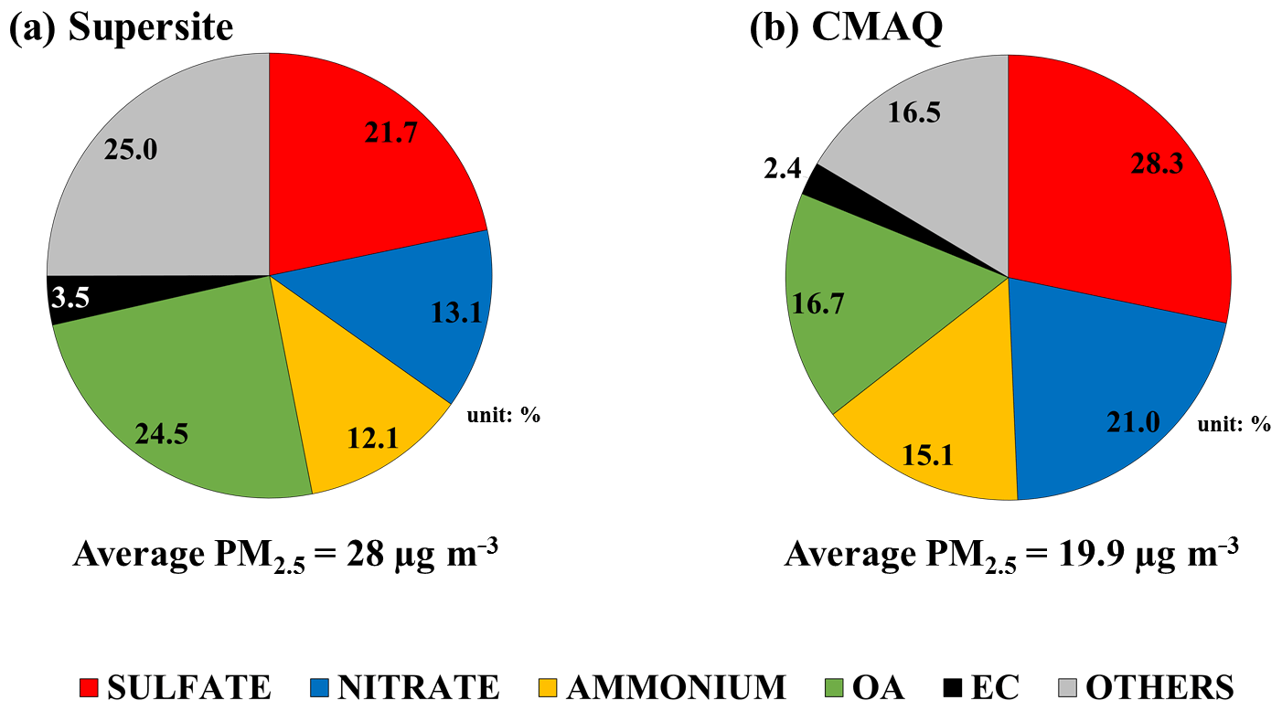
Figure 4Average PM2.5 composition (a) observed at the supersite stations and (b) simulated by the CMAQ model during the KORUS-AQ campaign. The averaged PM2.5 measured from the supersites and calculated from the CMAQ model simulations over the period of the KORUS-AQ campaign are 28 and 19.9 µg m−3, respectively. The mass of organic aerosols (OAs) was calculated by multiplying organic carbon mass by 1.6.
The performances of the air quality prediction system were evaluated by comparing them with ground-based observations from the Air Korea network and supersite stations in South Korea. Several sensitivity analyses were also conducted in order to assess the influences of the DA time intervals on the accuracy of the air quality prediction.
3.1 Evaluation of the air quality prediction system
3.1.1 Time-series analysis
Figure 5 shows the time-series plots of PM10, PM2.5, CO, O3 and SO2 concentrations from the BASE RUN and the DA RUN. Here, the observation data (OBS) obtained from the Air Korea network were compared with the results of the two sets of the CMAQ model simulations, i.e., (1) BASE RUN and (2) DA RUN. As mentioned previously, 20 % of the Air Korea observations used in the evaluation were randomly selected during the period of the KORUS-AQ campaign. The other 80 % of the Air Korea data were used in the DA at 00:00 UTC. For the forecast hours from 01:00 to 23:00 UTC, all of the ground observations (254 Air Korea and seven supersite stations) were used to evaluate the performances of the developed air quality prediction system. As shown in Fig. 5, we achieved some improvements in the prediction performances by applying the ICs to the CMAQ model simulations. The BASE RUN significantly underpredicted PM10, PM2.5 and CO, while the DA RUN produced concentrations that were more consistent with the observations than those of the BASE RUN.
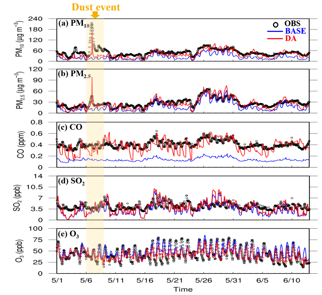
Figure 5Time-series plots of hourly (a) PM10, (b) PM2.5, (c) CO, (d) SO2 and (e) O3 concentrations at 264 Air Korea stations. Open black circles (OBS) represent the observed concentrations. Blue and red lines show the results simulated from the BASE RUN and DA RUN over South Korea, respectively.
In the case of CO, the observed CO mixing ratios were about 3 times higher than those from the BASE RUN. These large differences are well known and have been attributed to the underestimated emissions of CO (Heald et al., 2004). However, when the DA was applied, the predictions of the CO mixing ratios improved. Similarly, the performances of the PM10 and PM2.5 predictions improved with the application of the DA. Unlike PM10, PM2.5 and CO, the O3 mixing ratios and its diurnal trends from both the BASE RUN and DA RUN tend to be well matched with the observations. By contrast, the poorest performances of the BASE RUN and the DA RUN were shown for SO2.
In addition, a dust event took place between 6 and 8 May. This event is captured by the DA RUN (check red peaks in Fig. 5a and b), while the BASE RUN cannot capture this dust event. This demonstrates the capability of the current system to possibly predict dust events in South Korea. In the DA RUN, dust information is provided to the CMAQ model runs through both/either GOCI AOD and/or ground PM observations measured along the dust plume tracks.
The effectiveness of the DA with respect to prediction time was also analyzed by calculating the aggregated average concentrations of atmospheric species (see Figs. 6, 7 and 9). Figure 6 depicts the CMAQ-calculated average concentrations of PM10, PM2.5, CO and SO2 against the Air Korea observations. Our air quality prediction system regenerated relatively well-matched concentrations for PM10, PM2.5 and CO from the DA RUN.

Figure 6Aggregated average concentrations of (a) PM10, (b) PM2.5, (c) CO and (d) SO2 at 264 Air Korea stations over the KORUS-AQ campaign period. Open black circles denote the observations obtained from 264 Air Korea stations in South Korea. Blue and red lines represent the predicted concentrations from the BASE RUN and DA RUN, respectively. The DA was conducted at 00:00 UTC every day throughout the KORUS-AQ campaign period.
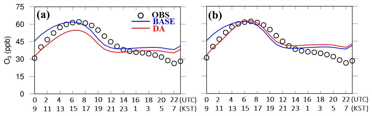
Figure 7Comparison of CMAQ-simulated O3 mixing ratios (BASE RUN with blue lines and DA RUN with red lines) with O3 mixing ratios from Air Korea stations (open black circles). DA RUN was carried out by assimilating CMAQ outputs with Air Korea observations using (a) only O3 mixing ratios and (b) both O3 and NO2 mixing ratios.
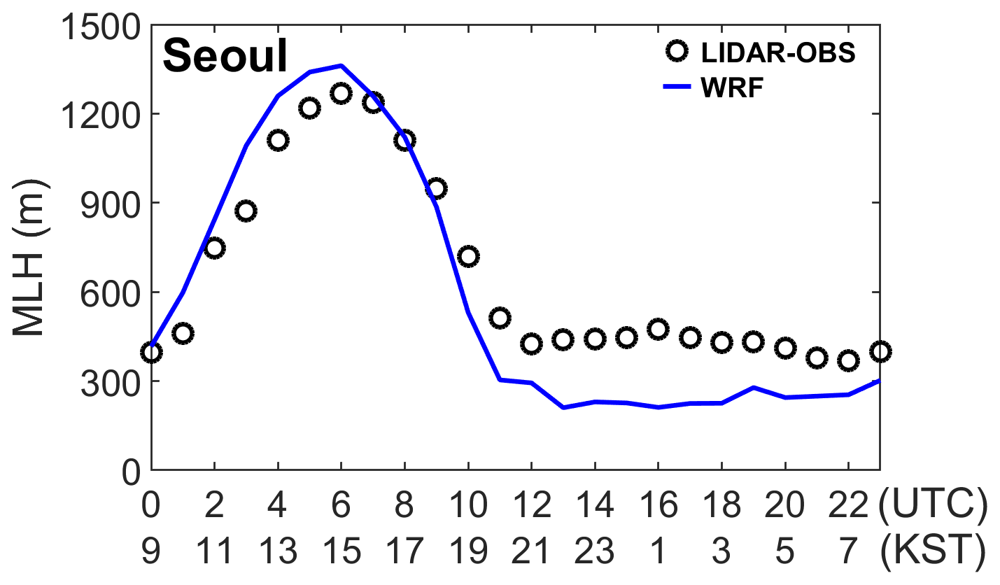
Figure 8Comparison of WRF-simulated mixing layer height (MLH) (denoted by dashed blue line) with lidar-measured MLH (denoted by open black circles) at Seoul National University (SNU) in Seoul. KST stands for Korean standard time.
Figure 7 shows the case of ozone from the DA RUN by assimilating CMAQ outputs with Air Korea-observed (a) O3 mixing ratios and (b) both O3 and NO2 mixing ratios for a preliminary test run. The ozone mixing ratios from the DA RUN in Fig. 7a were reasonably consistent with the observations at 00:00 UTC but disagreed with those between 04:00 and 09:00 UTC (13:00 and 18:00 KST), when solar insolation is the most intense. This may be attributed to the chemical imbalances between ozone production and ozone destruction (or titration). However, if CMAQ NO2 was assimilated with ground-based observations in South Korea (Air Korea) and China, the predicted ozone mixing ratios became substantially closer to the observations, as shown in Fig. 7b. This is clearly due to the fact that NOx is an important precursor of ozone. In the prediction of the ozone mixing ratios, both 1 h peak ozone (around 15:00 KST) and 8 h averaged ozone mixing ratios (between 09:00 and 17:00 KST) are important. Figure 7 clearly shows that the prediction accuracies of both the ozone mixing ratios were improved after the DA of NO2 mixing ratios.
Although the DA for NO2 provided better ozone predictions, one should take caution in using the NO2 observations. The NO2 mixing ratios measured at Air Korea sites are known to be contaminated by other nitrogen gases such as nitric acid (HNO3), peroxyacetyl nitrates (PANs) and alkyl nitrates (ANs), since the Air Korea NO2 mixing ratios are measured through a chemiluminescent method with catalysts of gold or molybdenum oxide at high temperatures. These are known to be “NO2 measurement artifacts” (Jung et al., 2017), which is one of the reasons that the DA of NO2 was not shown in Fig. 6. The NO2 mixing ratios are corrected from the Air Korea NO2 data and are then used to prepare the ICs via the DA for more accurate ozone and NO2 predictions. Currently, such corrections of the observed NO2 mixing ratios are being standardized with more sophisticated year-long NO2 measurements. After the corrections of the NO2 measurement artifacts, more evolved schemes of ozone and NO2 predictions will be possible in the future. As shown in Fig. 7, about a 20 % reduction (average fraction of non-NO2 mixing ratios in the observed NO2 mixing ratios) was made for these demonstration runs (Jung et al., 2017).
Another practical issue is now discussed. Although the assimilation with the observed NO2 mixing ratios can enhance the accuracy of the predictions of the daytime ozone mixing ratios, the nighttime ozone mixing ratios tend to be consistently overpredicted in the aggregated plot of the ozone mixing ratios at the observation sites (see Fig. 7). This can be caused by underestimated NO2 mixing ratios and thus not enough nighttime ozone titration. As mentioned before, reliable NO2 prediction via the correction of the NO2 measurement artifacts will be made in the future. Another possible reason of the overpredicted ozone mixing ratios during the nighttime can be underestimation of the mixing layer height (MLH). Figure 8 shows a comparison between lidar-measured MLH (black dashed line) and WRF-calculated MLH (with the option of the Yonsei University planetary boundary layer scheme by Hong et al., 2006; see red line). As shown in Fig. 8, the nocturnal lidar-measured MLH is about 2 times higher than the nocturnal WRF-calculated MLH as measured at a lidar site inside the campus of Seoul National University (SNU) in Seoul. Such underestimated MLH in the model tends to compress the ozone molecules within the mixing layer during the nighttime, which leads to consistently overpredicted nocturnal ozone mixing ratios. Based on this discrepancy shown in Fig. 8, more intensive comparison study is being carried out by comparing lidar-measured MLH with model-calculated MLH at multiple sites in South Korea.
In this work, the aerosol composition (including EC, OA, sulfate, nitrate and ammonium) was further compared with the composition observed at the supersites shown in Fig. 9. As shown in Fig. 9, agreement was observed between the DA RUN and observations for all of the major PM constituents. Again, a strong capability of our DA system is to improve the predictions of the aerosol composition.
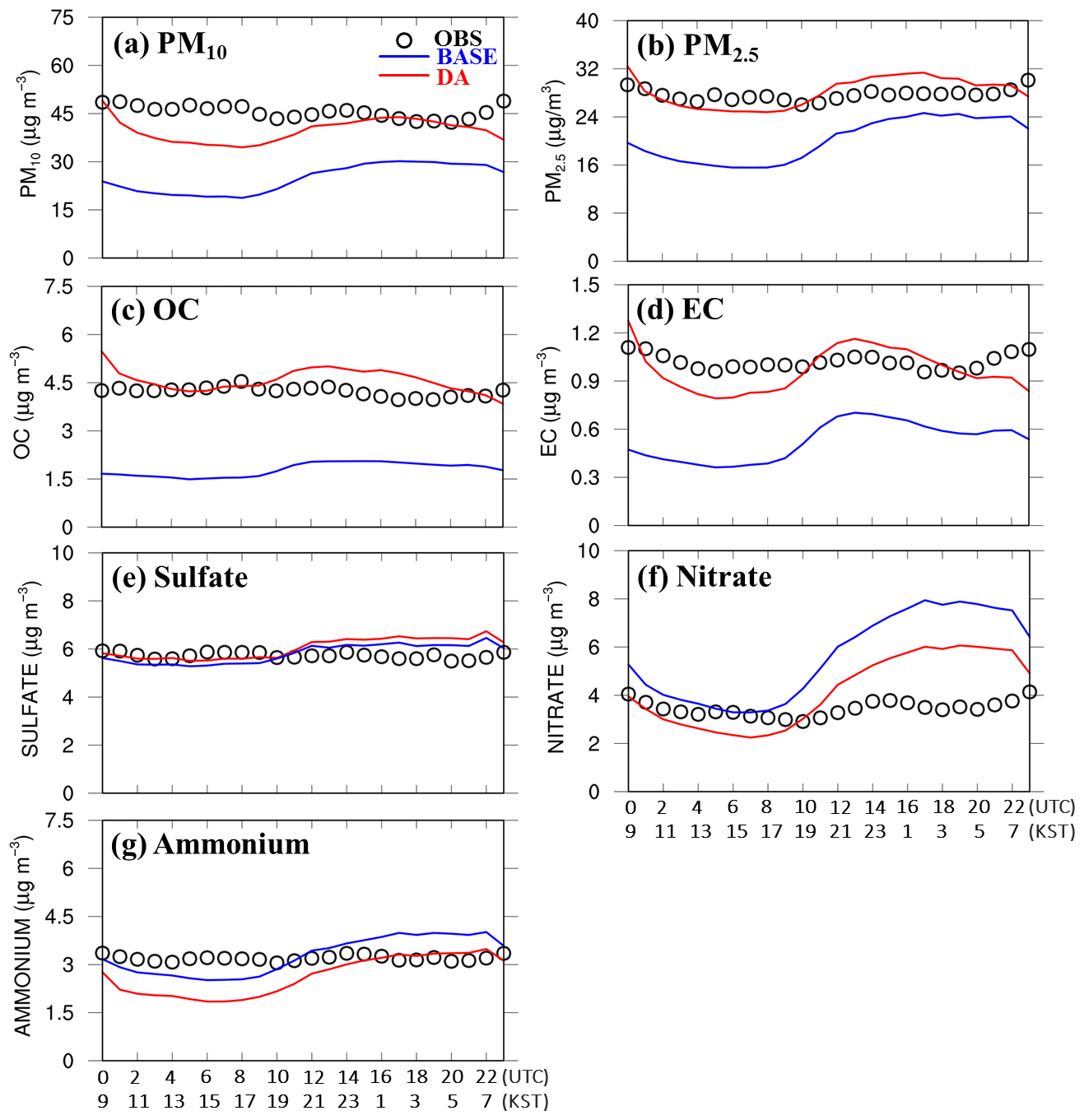
Figure 9Aggregated average concentrations of (a) PM10, (b) PM2.5, (c) OC, (d) EC, (e) sulfate, (f) nitrate and (g) ammonium as predicted by CMAQ model during the period of the KORUS-AQ campaign. The others are the same as those shown in Fig. 7, except for the fact that the observation data used here were obtained from the seven supersite stations in South Korea.
3.1.2 Spatial distribution
Figure 10 shows the spatial distributions and bias of PM and chemical species throughout the entire period of the KORUS-AQ campaign over the Seoul metropolitan area (SMA). Noticeable improvements are observed to have been achieved in the spatial distributions by applying the ICs to the CMAQ model simulations, particularly for PM10 (Fig. 10a), PM2.5 (Fig. 10b) and CO (Fig. 10c). As shown in Fig. 10, the underpredicted concentrations of PM10, PM2.5 and CO were adjusted to concentrations closer to the observations. In the case of SO2 (see Fig. 10d), the DA RUN produced better agreement with the observations than the BASE RUN, but there were still underpredicted SO2 concentrations over the northeastern part of the SMA.
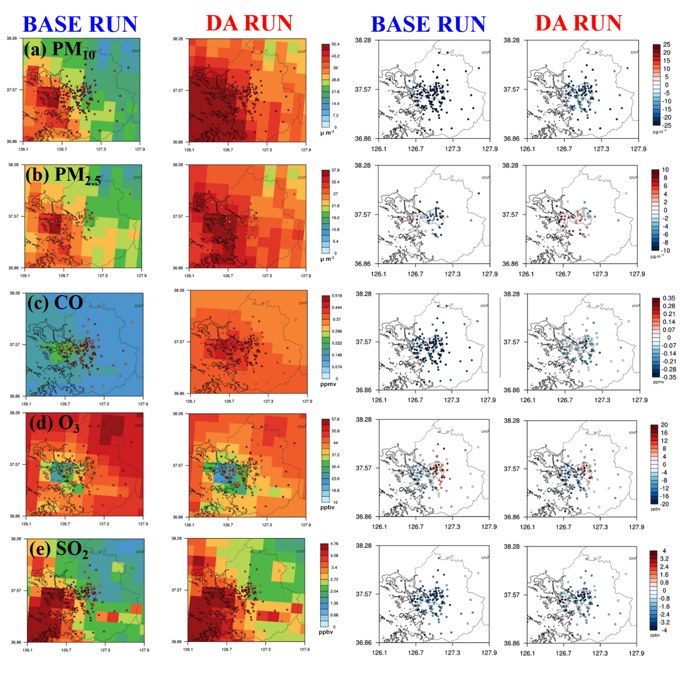
Figure 10Spatial distributions (first and second columns) and bias (third and fourth columns) of (a) PM10, (b) PM2.5, (c) CO, (d) O3 and (e) SO2 over Seoul metropolitan area (SMA) for the entire period of the KORUS-AQ campaign. Colored circles of first and second columns represent the concentrations of the air pollutants observed at the Air Korea stations in the SMA.
By contrast, relatively lower ozone mixing ratios from the DA RUN against the BASE RUN were found in the southwestern part of the SMA (see Fig. 10e). Due to the nonlinear relationship between NOx and O3, high mixing ratios (or emissions) of NOx in the SMA can lead to depletion of ozone. In these runs, the precursors of ozone such as NOx and volatile organic compounds (VOCs) were excluded in the preparation of the ICs for CMAQ model simulations. Again, this is because the Air Korea NO2 mixing ratios are contaminated by several reactive nitrogen species, so the data cannot be directly used in the assimilation procedures. In the case of VOCs, a limited number of datasets are available in South Korea for the DA. Improvements in the prediction of ozone mixing ratios can be achieved when the NO2 mixing ratios are corrected and a sufficient amount of VOC data (possibly from satellite data in the future) are available.
3.1.3 Statistical analysis
In order to achieve a better understanding of the performances of the DA RUN, analyses of statistical variables such as index of agreement (IOA), Pearson's correlation coefficient (R), root-mean-square error (RMSE) and mean bias (MB) were conducted using observations from the Air Korea stations for PM10, PM2.5, CO, SO2 and O3 (see Fig. 11). Definitions of the statistical variables are given in Appendix A.
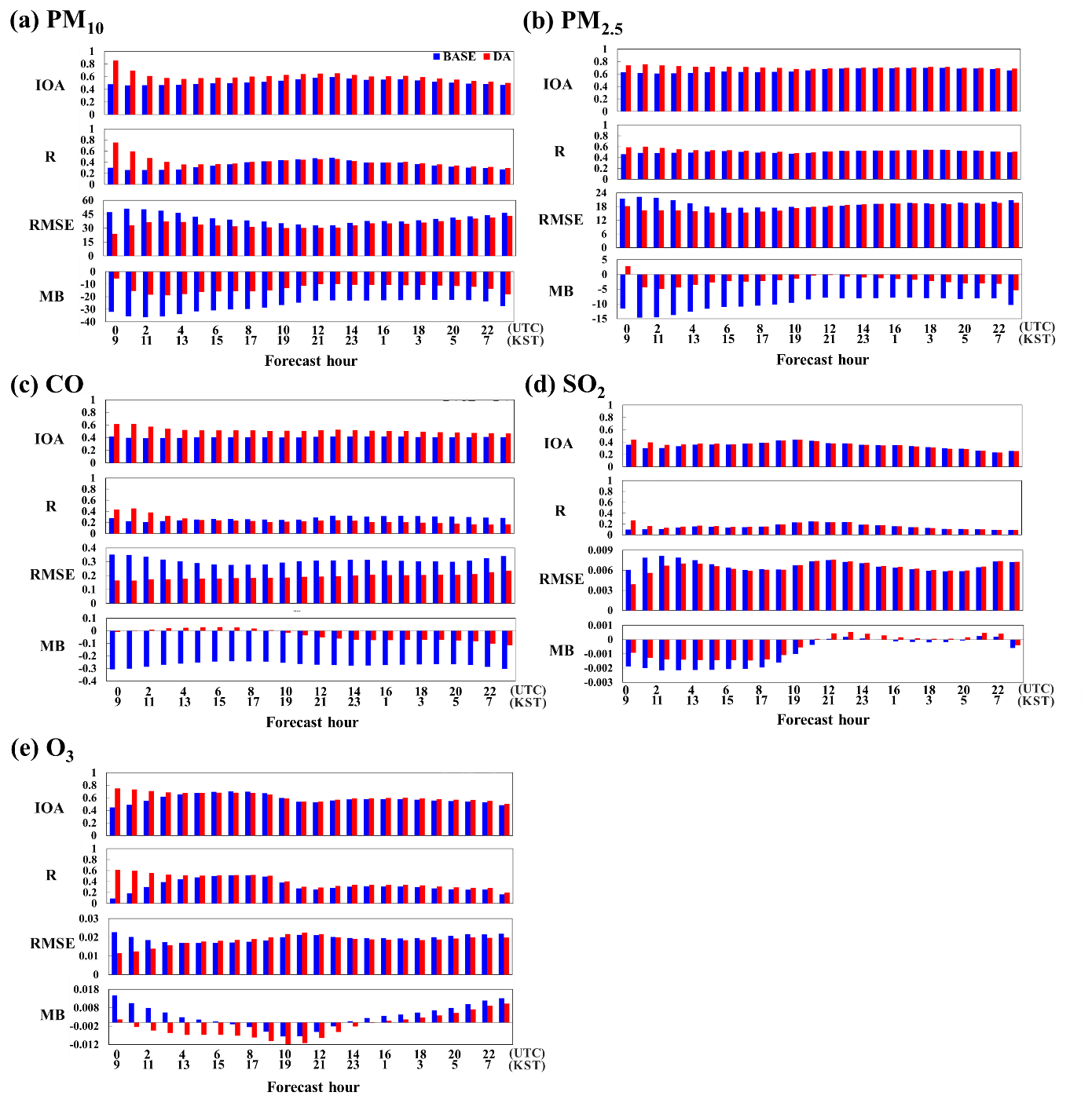
Figure 11Time-series plots of four performance metrics (IOA, R, RMSE and MB) for (a) PM10, (b) PM2.5, (c) CO, (d) SO2 and (e) O3 forecasts. The DA was conducted at 00:00 UTC. The units of RMSE and MB are micrograms per cubic meter and parts per million by volume for PM concentrations and for gaseous species, respectively. The definitions of the four performance metrics are shown in Appendix A.
After the applications of the ICs, both RMSE and MB became lower, while the correlation coefficient became higher for the entire set of predictions. In addition, it was found that the differences between the BASE RUN and the DA RUN tended to diminish as the prediction time progressed. The results of the statistical analysis are listed in Table 1. The results of the DA RUN were reasonably consistent with the observations for PM10 (IOA =0.60; R=0.40; RMSE =34.87; MB ) and PM2.5 (IOA =0.71; R=0.53; RMSE =17.83; MB ), as compared to the BASE RUN for PM10 (IOA =0.51; R=0.34; RMSE =40.84; MB ) and PM2.5 (IOA =0.67; R=0.51; RMSE =19.24; MB ). In terms of bias, an improvement was found for C, with MB = -0.036 for the DA RUN and MB for the BASE RUN. Regarding O3 and SO2, the DA RUN showed slightly better performances than the BASE RUN.
Table 1Statistical metrics from BASE RUN and DA RUN with Air Korea observations over the entire period of the KORUS-AQ campaign.
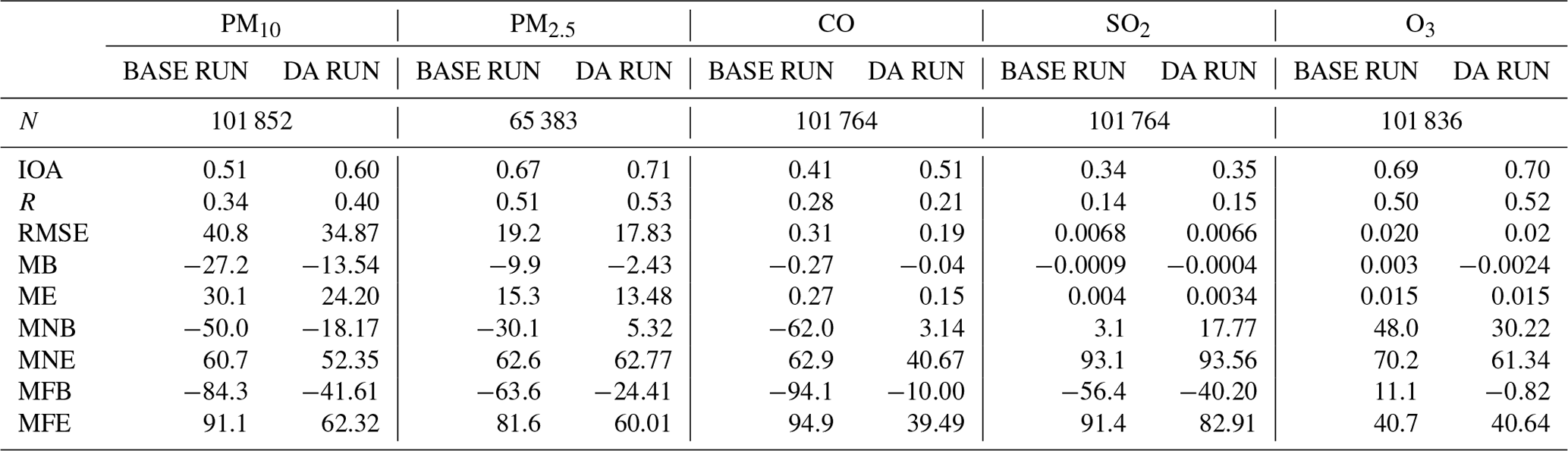
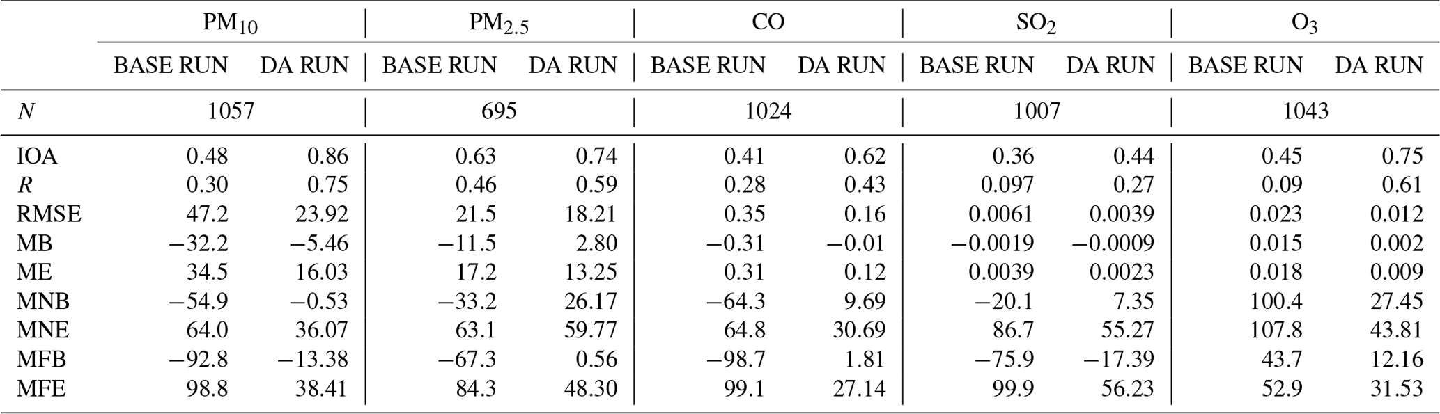
Table 2 presents the results of the statistical analysis at 00:00 UTC when the DA was conducted, with the results clearly showing how much closer the DA makes the CMAQ-calculated chemical concentrations to the observed concentrations. Collectively, the DA improved model accuracy by a large degree in terms of R, particularly for PM10 (R: 0.3→0.75; slope: 0.17→0.66) and O3 (R: 0.09→0.61; slope: 0.07→0.42). In addition, for all species, MB and RMSE decreased significantly with the DA RUN as compared with the BASE RUN.
Table 2Statistical metrics from BASE RUN and DA RUN with Air Korea observations at 00:00 UTC when the DA was conducted during the KORUS-AQ campaign.
3.2 Sensitivity test of DA time interval
3.2.1 AOD
In this section, a sensitivity analysis was conducted with different implementation time intervals of the DA (i.e., 24, 6 and 3 h) for AOD (refer to Fig. 12). As shown in Fig. 12, more frequent implementation of the DA is expected to make the predicted results closer to the observations. Although the DA RUN with a shorter assimilation time interval tends to produce a better prediction, it is not always the most appropriate choice, since the shorter assimilation time interval results in increased computational cost. Therefore, an optimized assimilation time interval should be found to achieve the best performances from the given DA system with the consideration of its own computational ability.
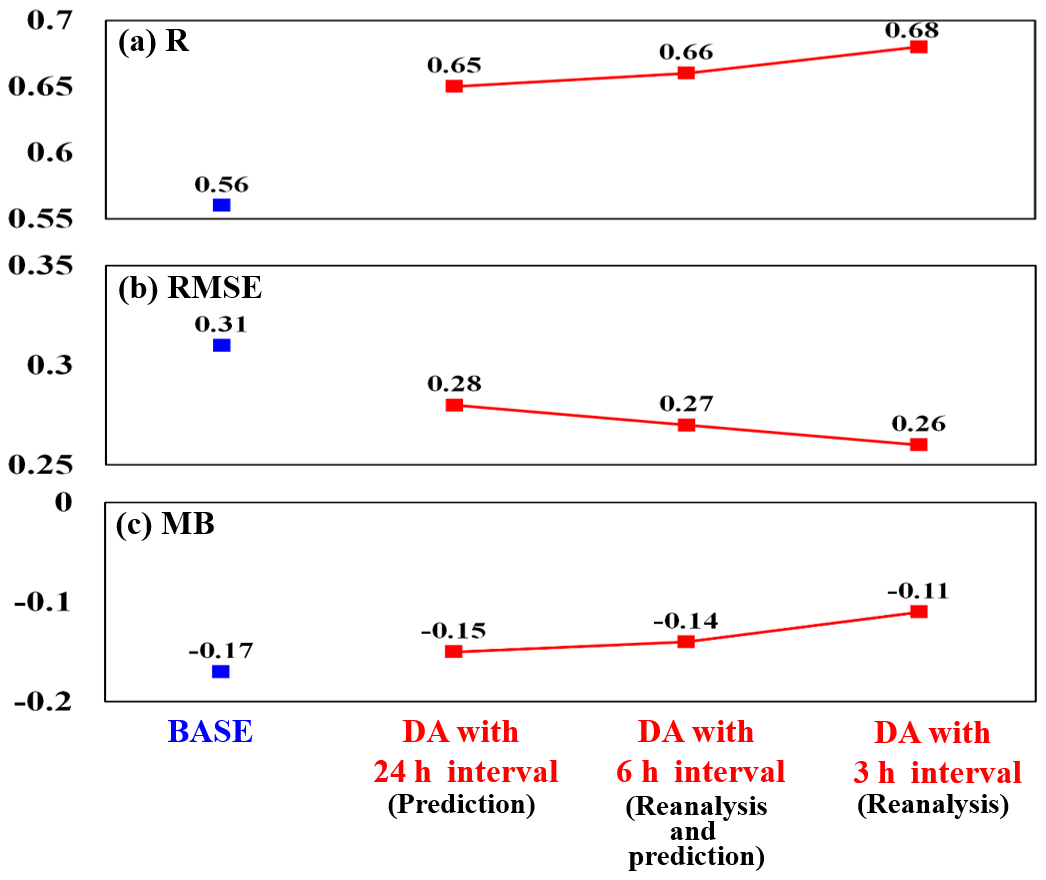
Figure 12Variations in three performance metrics (R, RMSE and MB) with time intervals of data assimilations. For these tests, the GOCI AODs were used in the DA to update the initial conditions of the CMAQ model simulations. The results from the three CMAQ model simulations were compared with AERONET AODs (“ground truth”). The blue squares represent the performances from the BASE RUNs and the red squares indicate the performances from the DA RUNs. The three experiments were carried out with the assimilation time intervals of 24, 6 and 3 h, respectively. Here, the DA RUN with the 24 h time interval is referred to as “air quality prediction”, and the DA RUNs with the 6 and 3 h time interval are referred to as “air quality reanalysis”.
3.2.2 PM and gases
In addition, sensitivity analyses of the developed air quality prediction system applied to multiple implementations of the DA with different time intervals were also investigated for (a) PM10, (b) PM2.5, (c) CO, (d) SO2 and (e) O3, shown in Fig. 13. Figure 13 shows a soccer plot analysis for BASE RUN (blue crosses) and DA RUNs with different DA time intervals of 24 h (OI; red circles), 2 h (2 h OI; black diamonds) and 1 h (1 h OI; dark-green triangles). This set of testing was designed based on the fact that the performances are expected to improve if the DAs are implemented multiple times prior to the actual predictions at 00:00 UTC. Here, for the 2 h OI run, the DA was implemented three times a day at 20:00, 22:00 and 00:00 UTC, while for the 1 h OI run, the DA was implemented at 22:00, 23:00 and 00:00 UTC. The performances of all of the chemical species excluding ozone improved, as expected, with DA RUNs with more frequent and longer DA time intervals (i.e., three-time implementation with a 2 h time interval in our cases). In the case of ozone, the best performance was found for the air quality prediction system with the DA time interval of 24 h.
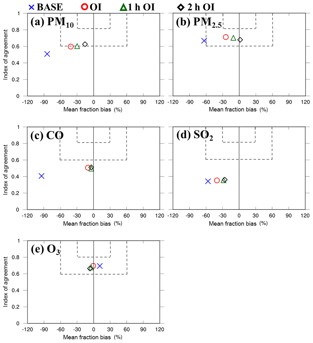
Figure 13Soccer plot analyses for (a) PM10, (b) PM2.5, (c) CO, (d) SO2 and (e) O3. The CMAQ-predicted concentrations were compared with the Air Korea observations. Blue crosses, red circles, dark-green triangles and black diamonds represent the performances calculated from the BASE RUN, the DA RUNs with the OI system, the 1 h OI system and the 2 h OI system, respectively.
Unsurprisingly, more frequent DAs prior to the actual prediction mode (i.e., before 00:00 UTC in our system) with a longer time interval (such as 2 h) will be computationally costly. There will certainly be a tradeoff between the precision of air quality prediction and the computational cost. The system should be designed under the consideration of these two factors.
In this study, the air quality prediction system was developed by preparing the ICs for CMAQ model simulations using GOCI AODs and ground-based observations of PM10, CO, ozone and SO2 during the period of the KORUS-AQ campaign (1 May–12 June 2016) in South Korea. The major advantages of the developed air quality prediction system are its comprehensiveness in predicting the ambient concentrations of both gaseous and particulate species (including PM composition) and its powerfulness in terms of computational cost. The performances of the developed prediction system were evaluated using near-surface in situ observation data. The CMAQ model runs with the ICs (DA RUN) showed higher consistency with the observations of almost all of the chemical species, including PM composition (sulfate, nitrate, ammonium, OA and EC) and atmospheric gases (CO, ozone and SO2), than the CMAQ model runs without the ICs (BASE RUN). Particularly for CO, the DA was able to remarkably improve the model performances, while the BASE RUN significantly underpredicted the CO concentrations (predicting about one-third of the observed values). In the case of ozone, both the BASE RUN and DA RUN were in close agreement with observations. More reliable predictions of ozone mixing ratios will be achieved via the DA of the observed NO2 mixing ratios and the corrections of model-simulated mixing layer height (MLH). For SO2, the performances of both the BASE RUN and the DA RUN were somewhat poor. Regarding this issue, more accurate SO2 emissions are required to achieve better SO2 predictions, and these can be estimated through inverse modeling using satellite data (e.g., Lee et al., 2011). The adjustments of both ICs and emissions may be able to improve the performances of the air quality prediction system, and this will be examined in future studies.
Moreover, the developed air quality prediction system will be upgraded by using the new observation data that will be retrieved after 2020 from the Geostationary Environment Monitoring Spectrometer (GEMS) with a high spatial resolution of 7 km×8 km as well as a high temporal resolution of 1 h over a large part of Asia. In addition, the current DA technique of the OI with the Kalman filter can also be upgraded with the use of more advanced DA methods such as variational techniques of 3DVAR and 4DVAR methods, as well as with the ensemble Kalman filter (EnK) method. These research endeavors are currently underway.
In conjunction with improving the air quality modeling system, artificial intelligence (AI)-based air quality prediction systems are also currently being developed in several ways (e.g., Kim et al., 2019). Actually, Kim et al. (2019) developed an AI-based PM prediction system based on a deep recurrent neural network (RNN) in South Korea. The AI-based prediction system was optimized by iterative model trainings with the inputs of ground-observed PM10, PM2.5, and meteorological fields including wind speed, wind direction, relative humidity, and precipitation. The AI-based prediction system showed better performances at several sites than the CMAQ model simulations. However, it works only for the observation sites in South Korea where ground-based observations are available. By taking advantage of both the CTM-based air quality prediction and the AI-based prediction systems, both systems will be eventually combined so as to create a more accurate hybrid air quality prediction system over South Korea. This will be the ultimate goal of the series of our research work.
The formulas used to evaluate the performances of the air quality prediction system are defined as follows:
In Eqs. (A1)–(A8), M and O represent the model and observation data, respectively. N is the number of data points, and σ means the standard deviation. The overbars in the equations indicate the arithmetic mean of the data. The units of RMSE and MB are the same as the unit of data, while IOA and R are dimensionless statistical parameters.
WRF v3.8.1 (https://doi.org/10.5065/D6MK6B4K, Skamarock et al., 2008) and CMAQ v5.1 (https://doi.org/10.5281/zenodo.1079909, US EPA Office of Research and Development, 2015) models are both open source and publicly available. Source codes for WRF and CMAQ can be downloaded at http://www2.mmm.ucar.edu/wrf/users/downloads.html (Skamarock et al., 2008) and https://github.com/USEPA/CMAQ (US EPA, 2020), respectively. Data from the KORUS-AQ field campaign can be downloaded from the KORUS-AQ data archive (http://www-air.larc.nasa.gov/missions/korus-aq, NASA, 2020a). Other data were acquired as follows. Ground-based observation data were downloaded from the Air Korea website (http://www.airkorea.or.kr, Korea Environment Corporation of the Ministry of Environment, 2020) for South Korea and from https://pm25.in (CNEMC, 2020) for China. AERONET data were downloaded from https://aeronet.gsfc.nasa.gov (NASA, 2020b). The KAQPS v1 (https://doi.org/10.5281/zenodo.3659551, Lee, 2020) code can be obtained by contacting Kyunghwa Lee (lkh1515@gmail.com) or from https://github.com/AIR-Codes/KAQPSv1 (Lee, 2020). NCL (2019; https://doi.org/10.5065/D6WD3XH5) was used to draw the figures.
KL developed the model code, performed the simulations and analyzed the results. CHS directed the experiments. JY contributed to shaping the research and analysis. SL, MP, HH and SYP helped analyze the results. MC, JK, YK, JH and SK provided and analyzed data applied in the experiments. KL prepared the paper with contributions from all coauthors.
The authors declare that they have no conflict of interest.
Special thanks go to the entire KORUS-AQ science team for their considerable efforts in conducting the campaign. Our thanks also go to the editor and anonymous reviewers for their constructive comments.
This research was supported by the National Strategic Project-Fine Particle of the National Research Foundation of Korea (NRF) of the Ministry of Science and ICT (MSIT), the Ministry of Environment (MOE), and the Ministry of Health and Welfare (MOHW) (grant no. NRF-2017M3D8A1092022). This work was also funded by the GEMS program of the MOE of the Republic of Korea as part of the Eco-Innovation Program of KEITI (grant no. 2012000160004) and was supported by a grant from the National Institute of Environment Research (NIER), funded by the MOE of the Republic of Korea (grant no. NIER-2019-01-01-028).
This paper was edited by Havala Pye and reviewed by two anonymous referees.
Adhikary, B., Kulkarni, S., Dallura, A., Tang, Y., Chai, T., Leung, L. R., Qian, Y., Chung, C. E., Ramanathan, V., and Carmichael, G. R.: A regional scale chemical transport modeling of Asian aerosols with data assimilation of AOD observations using optimal interpolation technique, Atmos. Environ., 42, 8600–8615, https://doi.org/10.1016/j.atmosenv.2008.08.031, 2008.
Appel, K. W., Roselle, S. J., Gilliam, R. C., and Pleim, J. E.: Sensitivity of the Community Multiscale Air Quality (CMAQ) model v4.7 results for the eastern United States to MM5 and WRF meteorological drivers, Geosci. Model Dev., 3, 169–188, https://doi.org/10.5194/gmd-3-169-2010, 2010.
Appel, K. W., Pouliot, G. A., Simon, H., Sarwar, G., Pye, H. O. T., Napelenok, S. L., Akhtar, F., and Roselle, S. J.: Evaluation of dust and trace metal estimates from the Community Multiscale Air Quality (CMAQ) model version 5.0, Geosci. Model Dev., 6, 883–899, https://doi.org/10.5194/gmd-6-883-2013, 2013.
Bellouin, N., Boucher, O., Haywood, J., and Reddy, M. S.: Global estimate of aerosol direct radiative forcing from satellite measurements, Nature, 438, 1138–1141, https://doi.org/10.1038/nature04348, 2005.
Breon, F.-M., Tanre, D., and Generoso, S.: Aerosol Effect on Cloud Droplet Size Monitored from Satellite, Science, 295, 834–838, https://doi.org/10.1126/science.1066434, 2002.
Byun, D. and Schere, K. L.: Review of the Governing Equations, Computational Algorithms, and Other Components of the Models-3 Community Multiscale Air Quality (CMAQ) Modeling System, Appl. Mech. Rev, 59, 51–77, https://doi.org/10.1115/1.2128636, 2006.
Byun, D. W. and Ching, J. K. S.: Science algorithms of the EPA models-3 community multiscale air quality (CMAQ) modeling system, U.S. Environmental Protection Agency, EPA/600/R-99/030 (NTIS PB2000-100561), 1999.
Carmichael, G. R., Sakurai, T., Streets, D., Hozumi, Y., Ueda, H., Park, S. U., Fung, C., Han, Z., Kajino, M., Engardt, M., Bennet, C., Hayami, H., Sartelet, K., Holloway, T., Wang, Z., Kannari, A., Fu, J., Matsuda, K., Thongboonchoo, N., and Amann, M.: MICS-Asia II: The model intercomparison study for Asia Phase II methodology and overview of findings, Atmos. Environ., 42, 3468–3490, https://doi.org/10.1016/j.atmosenv.2007.04.007, 2008.
Carmichael, G. R., Adhikary, B., Kulkarni, S., D'Allura, A., Tang, Y., Streets, D., Zhang, Q., Bond, T. C., Ramanathan, V., Jamroensan, A., and Marrapu, P.: Asian Aerosols: Current and Year 2030 Distributions and Implications to Human Health and Regional Climate Change, Environ. Sci. Technol., 43, 5811–5817, https://doi.org/10.1021/es8036803, 2009.
Chemel, C., Sokhi, R. S., Yu, Y., Hayman, G. D., Vincent, K. J., Dore, A. J., Tang, Y. S., Prain, H. D., and Fisher, B. E. A.: Evaluation of a CMAQ simulation at high resolution over the UK for the calendar year 2003, Atmos. Environ., 44, 2927–2939, https://doi.org/10.1016/j.atmosenv.2010.03.029, 2010.
Chin, M., Ginoux, P., Kinne, S., Torres, O., Holben, B. N., Duncan, B. N., Martin, R. V., Logan, J. A., Higurashi, A., and Nakajima, T.: Tropospheric Aerosol Optical Thickness from the GOCART Model and Comparisons with Satellite and Sun Photometer Measurements, J. Atmos. Sci., 59, 461–483, https://doi.org/10.1175/1520-0469(2002)059<0461:TAOTFT>2.0.CO;2, 2002.
Chinese monitoring network of the China National Environmental Monitoring Center (CNEMC): PM2.5 in China, available at: https://pm25.in, last access: 8 March 2020.
Choi, M., Kim, J., Lee, J., Kim, M., Park, Y.-J., Jeong, U., Kim, W., Hong, H., Holben, B., Eck, T. F., Song, C. H., Lim, J.-H., and Song, C.-K.: GOCI Yonsei Aerosol Retrieval (YAER) algorithm and validation during the DRAGON-NE Asia 2012 campaign, Atmos. Meas. Tech., 9, 1377–1398, https://doi.org/10.5194/amt-9-1377-2016, 2016.
Choi, M., Kim, J., Lee, J., Kim, M., Park, Y.-J., Holben, B., Eck, T. F., Li, Z., and Song, C. H.: GOCI Yonsei aerosol retrieval version 2 products: an improved algorithm and error analysis with uncertainty estimation from 5-year validation over East Asia, Atmos. Meas. Tech., 11, 385–408, https://doi.org/10.5194/amt-11-385-2018, 2018.
Chung, C. E., Ramanathan, V., Carmichael, G., Kulkarni, S., Tang, Y., Adhikary, B., Leung, L. R., and Qian, Y.: Anthropogenic aerosol radiative forcing in Asia derived from regional models with atmospheric and aerosol data assimilation, Atmos. Chem. Phys., 10, 6007–6024, https://doi.org/10.5194/acp-10-6007-2010, 2010.
Colella, P. and Woodward, P. R.: The Piecewise Parabolic Method (PPM) for gas-dynamical simulations, J. Comput. Phys., 54, 174–201, https://doi.org/10.1016/0021-9991(84)90143-8, 1984.
Collins, W. D., Rasch, P. J., Eaton, B. E., Khattatov, B. V., Lamarque, J.-F., and Zender, C. S.: Simulating aerosols using a chemical transport model with assimilation of satellite aerosol retrievals: Methodology for INDOEX, J. Geophys. Res., 106, 7313–7336, https://doi.org/10.1029/2000JD900507, 2001.
Cressman, G. P.: An operational objective analysis system, Mon. Weather Rev., 87, 367–374, 1959.
Dehghani, M., Keshtgar, L., Javaheri, M. R., Derakhshan, Z., Conti, O., Gea, Zuccarello, P., and Ferrante, M.: The effects of air pollutants on the mortality rate of lung cancer and leukemia, Mol. Med. Rep., 15, 3390–3397, 2017.
Emmons, L. K., Walters, S., Hess, P. G., Lamarque, J.-F., Pfister, G. G., Fillmore, D., Granier, C., Guenther, A., Kinnison, D., Laepple, T., Orlando, J., Tie, X., Tyndall, G., Wiedinmyer, C., Baughcum, S. L., and Kloster, S.: Description and evaluation of the Model for Ozone and Related chemical Tracers, version 4 (MOZART-4), Geosci. Model Dev., 3, 43–67, https://doi.org/10.5194/gmd-3-43-2010, 2010.
Foley, K. M., Roselle, S. J., Appel, K. W., Bhave, P. V., Pleim, J. E., Otte, T. L., Mathur, R., Sarwar, G., Young, J. O., Gilliam, R. C., Nolte, C. G., Kelly, J. T., Gilliland, A. B., and Bash, J. O.: Incremental testing of the Community Multiscale Air Quality (CMAQ) modeling system version 4.7, Geosci. Model Dev., 3, 205–226, https://doi.org/10.5194/gmd-3-205-2010, 2010.
Friedl, M. A., Sulla-Menashe, D., Tan, B., Schneider, A., Ramankutty, N., Sibley, A., and Huang, X.: MODIS Collection 5 global land cover: Algorithm refinements and characterization of new datasets, Remote Sens. Environ., 114, 168–182, https://doi.org/10.1016/j.rse.2009.08.016, 2010.
Generoso, S., Breon, F.-M., Chevallier, F., Balkanski, Y., Schulz, M., and Bey, I.: Assimilation of POLDER aerosol optical thickness into the LMDz-INCA model: Implications for the Arctic aerosol burden, J. Geophys. Res., 112, D02311, https://doi.org/10.1029/2005JD006954, 2007.
Grell, G. A. and Freitas, S. R.: A scale and aerosol aware stochastic convective parameterization for weather and air quality modeling, Atmos. Chem. Phys., 14, 5233–5250, https://doi.org/10.5194/acp-14-5233-2014, 2014.
Guenther, A., Karl, T., Harley, P., Wiedinmyer, C., Palmer, P. I., and Geron, C.: Estimates of global terrestrial isoprene emissions using MEGAN (Model of Emissions of Gases and Aerosols from Nature), Atmos. Chem. Phys., 6, 3181–3210, https://doi.org/10.5194/acp-6-3181-2006, 2006.
Guenther, A. B., Jiang, X., Heald, C. L., Sakulyanontvittaya, T., Duhl, T., Emmons, L. K., and Wang, X.: The Model of Emissions of Gases and Aerosols from Nature version 2.1 (MEGAN2.1): an extended and updated framework for modeling biogenic emissions, Geosci. Model Dev., 5, 1471–1492, https://doi.org/10.5194/gmd-5-1471-2012, 2012.
Heald, C. L., Jacob, D. J., Jones, D. B. A., Palmer, P. I., Logan, J. A., Streets, D. G., Sachse, G. W., Gille, J. C., Hoffman, R. N., and Nehrkorn, T.: Comparative inverse analysis of satellite (MOPITT) and aircraft (TRACE-P) observations to estimate Asian sources of carbon monoxide: Comparative inverse analysis, J. Geophys. Res.-Atmos., 109, D23306, https://doi.org/10.1029/2004JD005185, 2004.
Hertel, O., Berkowicz, R., Christensen, J. and Hov, Ø.: Test of two numerical schemes for use in atmospheric transport-chemistry models, Atmos. Environ., 27, 2591–2611, https://doi.org/10.1016/0960-1686(93)90032-T, 1993.
Holben, B. N., Eck, T. F., Slutsker, I., Tanre, D., Buis, J. P., Setzer, A., Vermote, E., Reagan, J. A., Kaufman, Y. J., Nakajima, T., Lavenu, F., Jankowiak, I., and Smirnov, A.: AERONET – A Federated Instrument Network and Data Archive for Aerosol Characterization, Remote Sens. Environ., 66, 1–16, https://doi.org/10.1016/S0034-4257(98)00031-5, 1998.
Hong, S.-Y. and Lim, J.-O. J.: The WRF single-moment 6-class microphysics scheme (WSM6), J. Korean Meteor. Soc., 42, 129–151, 2006.
Hong, S.-Y., Noh, Y., and Dudhia, J.: A New Vertical Diffusion Package with an Explicit Treatment of Entrainment Processes, Mon. Weather Rev., 134, 2318–2341, https://doi.org/10.1175/MWR3199.1, 2006.
Hutzell, W. T., Luecken, D. J., Appel, K. W., and Carter, W. P. L.: Interpreting predictions from the SAPRC07 mechanism based on regional and continental simulations, Atmos. Environ., 46, 417–429, https://doi.org/10.1016/j.atmosenv.2011.09.030, 2012.
Iacono, M. J., Delamere, J. S., Mlawer, E. J., Shephard, M. W., Clough, S. A., and Collins, W. D.: Radiative forcing by long-lived greenhouse gases: Calculations with the AER radiative transfer models, J. Geophys. Res., 113, D13103, https://doi.org/10.1029/2008JD009944, 2008.
IPCC: Climate Change 2013: The Physical Science Basis. The Fifth Assessment Report of the Intergovernmental Panel on Climate Change, Cambridge University Press, Cambridge, United Kingdom and New York, NY, USA, 2013.
Jimenez, P. A., Dudhia, J., Gonzalez-Rouco, J. F., Navarro, J., Montavez, J. P., and Garcia-Bustamante, E.: A Revised Scheme for the WRF Surface Layer Formulation, Mon. Weather Rev., 140, 898–918, 2012.
Jung, J., Lee, J., Kim, B., and Oh, S.: Seasonal variations in the NO2 artifact from chemiluminescence measurements with a molybdenum converter at a suburban site in Korea (downwind of the Asian continental outflow) during 2015–2016, Atmos. Environ., 165, 290–300, https://doi.org/10.1016/j.atmosenv.2017.07.010, 2017.
Khaniabadi, Y. O., Goudarzi, G., Daryanoosh, S. M., Borgini, A., Tittarelli, A., and De Marco, A.: Exposure to PM10, NO2, and O3 and impacts on human health, Environ. Sci. Pollut. Res., 24, 2781–2789, https://doi.org/10.1007/s11356-016-8038-6, 2017.
Khattatov, B. V., Gille, J. C., Lyjak, L. V., Brasseur, G. P., Dvortsov, V. L., Roche, A. E., and Waters, J. W.: Assimilation of photochemically active species and a case analysis of UARS data, J. Geophys. Res., 104, 18715–18737, https://doi.org/10.1029/1999JD900225, 1999.
Khattatov, B. V., Lamarque, J.-F., Lyjak, L. V., Menard, R., Levelt, P., Tie, X., Brasseur, G. P., and Gille, J. C.: Assimilation of satellite observations of long-lived chemical species in global chemistry transport models, J. Geophys. Res., 105, 29135–29144, https://doi.org/10.1029/2000JD900466, 2000.
Kim, H. S., Park, I., Song, C. H., Lee, K., Yun, J. W., Kim, H. K., Jeon, M., Lee, J., and Han, K. M.: Development of a daily PM10 and PM2.5 prediction system using a deep long short-term memory neural network model, Atmos. Chem. Phys., 19, 12935–12951, https://doi.org/10.5194/acp-19-12935-2019, 2019.
Korea Environment Corporation of the Ministry of Environment: Air Korea, available at: http://www.airkorea.or.kr, last access: 8 March 2020.
Lamarque, J.-F., Khattatov, B. V., Gille, J. C., and Brasseur, G. P.: Assimilation of Measurement of Air Pollution from Space (MAPS) CO in a global three-dimensional model, J. Geophys. Res., 104, 26209–26218, https://doi.org/10.1029/1999JD900807, 1999.
Lee, C., Martin, R. V., Donkelaar, A. van, Lee, H., Dickerson, R. R., Hains, J. C., Krotkov, N., Richter, A., Vinnikov, K., and Schwab, J. J.: SO2 emissions and lifetimes: Estimates from inverse modeling using in situ and global, space-based (SCIAMACHY and OMI) observations, J. Geophys. Res.-Atmos., 116, D06304, https://doi.org/10.1029/2010JD014758, 2011.
Lee, J., Kim, J., Song, C. H., Ryu, J.-H., Ahn, Y.-H., and Song, C. K.: Algorithm for retrieval of aerosol optical properties over the ocean from the Geostationary Ocean Color Imager, Remote Sens. Environ., 114, 1077–1088, https://doi.org/10.1016/j.rse.2009.12.021, 2010.
Lee, J., Kim, J., Yang, P., and Hsu, N. C.: Improvement of aerosol optical depth retrieval from MODIS spectral reflectance over the global ocean using new aerosol models archived from AERONET inversion data and tri-axial ellipsoidal dust database, Atmos. Chem. Phys., 12, 7087–7102, https://doi.org/10.5194/acp-12-7087-2012, 2012.
Lee, K.: AIR-Codes/KAQPS: Korean Air Quality Prediction System (Version v1.0), Zenodo, https://doi.org/10.5281/zenodo.3659551, 2020.
Lee, S., Song, C. H., Park, R. S., Park, M. E., Han, K. M., Kim, J., Choi, M., Ghim, Y. S., and Woo, J.-H.: GIST-PM-Asia v1: development of a numerical system to improve particulate matter forecasts in South Korea using geostationary satellite-retrieved aerosol optical data over Northeast Asia, Geosci. Model Dev., 9, 17–39, https://doi.org/10.5194/gmd-9-17-2016, 2016.
Levelt, P. F., Khattatov, B. V., Gille, J. C., Brasseur, G. P., Tie, X. X., and Waters, J. W.: Assimilation of MLS ozone measurements in the global three-dimensional chemistry transport model ROSE, Geophys. Res. Lett., 25, 4493–4496, https://doi.org/10.1029/1998GL900152, 1998.
Lorenc, A. C.: Analysis methods for numerical weather prediction, Q. J. Roy. Meteor. Soc., 112, 1177–1194, https://doi.org/10.1002/qj.49711247414, 1986.
Louis, J.-F.: A parametric model of vertical eddy fluxes in the atmosphere, Bound.-Lay. Meteorol., 17, 187–202, https://doi.org/10.1007/BF00117978, 1979.
Malm, W. C. and Hand, J. L.: An examination of the physical and optical properties of aerosols collected in the IMPROVE program, Atmos. Environ., 41, 3407–3427, https://doi.org/10.1016/j.atmosenv.2006.12.012, 2007.
Martin, R. V., Jacob, D. J., Yantosca, R. M., Chin, M., and Ginoux, P.: Global and regional decreases in tropospheric oxidants from photochemical effects of aerosols, J. Geophys. Res., 108, 4097, https://doi.org/10.1029/2002JD002622, 2003.
NASA: KORUS-AQ, available at: http://www-air.larc.nasa.gov/missions/korus-aq, last access: 8 March 2020a.
NASA: AERONET, available at: https://aeronet.gsfc.nasa.gov, last access: 8 March 2020b.
NCL: The NCAR Command Language (Version 6.6.2) [Software], Boulder, Colorado, UCAR/NCAR/CISL/TDD, https://doi.org/10.5065/D6WD3XH5, 2019.
Niu, G.-Y., Yang, Z.-L., Mitchell, Kenneth. E., Chen, F., Ek, M. B., Barlage, M., Kumar, A., Manning, K., Niyogi, D., Rosero, E., Tewari, M., and Xia, Y.: The community Noah land surface model with multiparameterization options (Noah-MP): 1. Model description and evaluation with local-scale measurements, J. Geophys. Res., 116, D12109, https://doi.org/10.1029/2010JD015140, 2011.
Otte, T. L. and Pleim, J. E.: The Meteorology-Chemistry Interface Processor (MCIP) for the CMAQ modeling system: updates through MCIPv3.4.1, Geosci. Model Dev., 3, 243–256, https://doi.org/10.5194/gmd-3-243-2010, 2010.
Park, M. E., Song, C. H., Park, R. S., Lee, J., Kim, J., Lee, S., Woo, J.-H., Carmichael, G. R., Eck, T. F., Holben, B. N., Lee, S.-S., Song, C. K., and Hong, Y. D.: New approach to monitor transboundary particulate pollution over Northeast Asia, Atmos. Chem. Phys., 14, 659–674, https://doi.org/10.5194/acp-14-659-2014, 2014.
Park, R. S., Song, C. H., Han, K. M., Park, M. E., Lee, S.-S., Kim, S.-B., and Shimizu, A.: A study on the aerosol optical properties over East Asia using a combination of CMAQ-simulated aerosol optical properties and remote-sensing data via a data assimilation technique, Atmos. Chem. Phys., 11, 12275–12296, https://doi.org/10.5194/acp-11-12275-2011, 2011.
Penner, J. E., Dong, X., and Chen, Y.: Observational evidence of a change in radiative forcing due to the indirect aerosol effect, Nature, 427, 231–234, https://doi.org/10.1038/nature02234, 2004.
Pleim, J. E.: A Combined Local and Nonlocal Closure Model for the Atmospheric Boundary Layer, Part I: Model Description and Testing, J. Appl. Meteorol. Clim., 46, 1383–1395, https://doi.org/10.1175/JAM2539.1, 2007a.
Pleim, J. E.: A Combined Local and Nonlocal Closure Model for the Atmospheric Boundary Layer. Part II: Application and Evaluation in a Mesoscale Meteorological Model, J. Appl. Meteorol. Clim., 46, 1396–1409, https://doi.org/10.1175/JAM2534.1, 2007b.
Pleim, J. E. and Xiu, A.: Development of a Land Surface Model. Part II: Data Assimilation, J. Appl. Meteorol., 42, 1811–1822, https://doi.org/10.1175/1520-0450(2003)042<1811:DOALSM>2.0.CO;2, 2003.
Scott, C. E., Rap, A., Spracklen, D. V., Forster, P. M., Carslaw, K. S., Mann, G. W., Pringle, K. J., Kivekäs, N., Kulmala, M., Lihavainen, H., and Tunved, P.: The direct and indirect radiative effects of biogenic secondary organic aerosol, Atmos. Chem. Phys., 14, 447–470, https://doi.org/10.5194/acp-14-447-2014, 2014.
Skamarock, C., Klemp, B., Dudhia, J., Gill, O., Barker, D., Duda, G., Huang, X., Wang, W., and Powers, G.: A Description of the Advanced Research WRF Version 3, https://doi.org/10.5065/D68S4MVH, 2008.
Tang, Y., Chai, T., Pan, L., Lee, P., Tong, D., Kim, H.-C., and Chen, W.: Using optimal interpolation to assimilate surface measurements and satellite AOD for ozone and PM2.5: A case study for July 2011, J. Air Waste Manage., 65, 1206–1216, https://doi.org/10.1080/10962247.2015.1062439, 2015.
Tang, Y., Pagowski, M., Chai, T., Pan, L., Lee, P., Baker, B., Kumar, R., Delle Monache, L., Tong, D., and Kim, H.-C.: A case study of aerosol data assimilation with the Community Multi-scale Air Quality Model over the contiguous United States using 3D-Var and optimal interpolation methods, Geosci. Model Dev., 10, 4743–4758, https://doi.org/10.5194/gmd-10-4743-2017, 2017.
US EPA: CMAQ Download, available at: https://github.com/USEPA/CMAQ, last access: 8 March 2020.
US EPA Office of Research and Development: CMAQv5.1 (Version 5.1), Zenodo, https://doi.org/10.5281/zenodo.1079909, 2015.
Wiedinmyer, C., Quayle, B., Geron, C., Belote, A., McKenzie, D., Zhang, X., O'Neill, S., and Wynne, K. K.: Estimating emissions from fires in North America for air quality modeling, Atmos. Environ., 40, 3419–3432, https://doi.org/10.1016/j.atmosenv.2006.02.010, 2006.
Wiedinmyer, C., Akagi, S. K., Yokelson, R. J., Emmons, L. K., Al-Saadi, J. A., Orlando, J. J., and Soja, A. J.: The Fire INventory from NCAR (FINN): a high resolution global model to estimate the emissions from open burning, Geosci. Model Dev., 4, 625–641, https://doi.org/10.5194/gmd-4-625-2011, 2011.
Woo, J.-H., Choi, K.-C., Kim, H. K., Baek, B. H., Jang, M., Eum, J.-H., Song, C. H., Ma, Y.-I., Sunwoo, Y., Chang, L.-S., and Yoo, S. H.: Development of an anthropogenic emissions processing system for Asia using SMOKE, Atmos. Environ., 58, 5–13, https://doi.org/10.1016/j.atmosenv.2011.10.042, 2012.
Xiu, A. and Pleim, J. E.: Development of a Land Surface Model, Part I: Application in a Mesoscale Meteorological Model, J. Appl. Meteorol., 40, 192–209, https://doi.org/10.1175/1520-0450(2001)040<0192:DOALSM>2.0.CO;2, 2001.
Yang, Z.-L., Niu, G.-Y., Mitchell, K. E., Chen, F., Ek, M. B., Barlage, M., Longuevergne, L., Manning, K., Niyogi, D., Tewari, M., and Xia, Y.: The community Noah land surface model with multiparameterization options (Noah-MP): 2. Evaluation over global river basins, J. Geophys. Res., 116, D12110, https://doi.org/10.1029/2010JD015139, 2011.
Yu, H., Dickinson, R. E., Chin, M., Kaufman, Y. J., Holben, B. N., Geogdzhayev, I. V., and Mishchenko, M. I.: Annual cycle of global distributions of aerosol optical depth from integration of MODIS retrievals and GOCART model simulations, J. Geophys. Res., 108, 4128, https://doi.org/10.1029/2002JD002717, 2003.
Yuan, H., Dai, Y., Xiao, Z., Ji, D., and Shangguan, W.: Reprocessing the MODIS Leaf Area Index products for land surface and climate modelling, Remote Sens. Environ., 115, 1171–1187, https://doi.org/10.1016/j.rse.2011.01.001, 2011.