the Creative Commons Attribution 4.0 License.
the Creative Commons Attribution 4.0 License.
 | 12 Mar 2019
ATAT 1.1, the Automated Timing Accordance Tool for comparing ice-sheet model output with geochronological data
Chris D. Clark
David Small
Richard C. A. Hindmarsh
Earth's extant ice sheets are of great societal importance given their ongoing and potential future contributions to sea-level rise. Numerical models of ice sheets are designed to simulate ice-sheet behaviour in response to climate changes but to be improved require validation against observations. The direct observational record of extant ice sheets is limited to a few recent decades, but there is a large and growing body of geochronological evidence spanning millennia constraining the behaviour of palaeo-ice sheets. Hindcasts can be used to improve model formulations and study interactions between ice sheets, the climate system and landscape. However, ice-sheet modelling results have inherent quantitative errors stemming from parameter uncertainty and their internal dynamics, leading many modellers to perform ensemble simulations, while uncertainty in geochronological evidence necessitates expert interpretation. Quantitative tools are essential to examine which members of an ice-sheet model ensemble best fit the constraints provided by geochronological data. We present the Automated Timing Accordance Tool (ATAT version 1.1) used to quantify differences between model results and geochronological data on the timing of ice-sheet advance and/or retreat. To demonstrate its utility, we perform three simplified ice-sheet modelling experiments of the former British–Irish ice sheet. These illustrate how ATAT can be used to quantify model performance, either by using the discrete locations where the data originated together with dating constraints or by comparing model outputs with empirically derived reconstructions that have used these data along with wider expert knowledge. The ATAT code is made available and can be used by ice-sheet modellers to quantify the goodness of fit of hindcasts. ATAT may also be useful for highlighting data inconsistent with glaciological principles or reconstructions that cannot be replicated by an ice-sheet model.
- Article
(8395 KB) - Full-text XML
-
Supplement
(72 KB) - BibTeX
- EndNote


Numerical models have been developed which simulate ice sheets under a given climate forcing (e.g. Greve and Hutter, 1995; Rutt et al., 2009; Pollard and DeConto, 2009; Winkelmann et al., 2011; Gudmundsson et al., 2012; Cornford et al., 2013; Pattyn, 2017). When driven by future climate scenarios, these models are used to forecast the fate of the Antarctic and Greenland ice sheets (e.g. Seddik et al., 2012; DeConto and Pollard, 2016), providing predictions of their potential contribution to future sea-level rise. However, incomplete knowledge of ice physics, boundary conditions (e.g. basal topography) and parameterisations of physical processes (e.g. basal sliding, calving), as well as the difficulty of predicting future climate, lead to model-based uncertainty in these predictions (Applegate et al., 2012; Briggs et al., 2014; Ritz et al., 2015). Observations of ice-marginal fluctuations (decades) and the processes of ice calving, flow or melting (subaerial or submarine) that facilitate or drive such variations, provide a powerful means to understand the processes leading to the possibility of deriving new formulations that improve the realism of modelling. However, the short time span (decades) of these observations limits their use to constrain, initialise or validate modelling experiments (Bamber and Aspinall, 2013). Conversely, palaeo-ice sheets, especially from the last glaciation (∼21 000 years ago), left behind evidence which provides the opportunity to study ice-sheet variations across timescales of centuries to millennia, albeit with increased uncertainty in exact timing.
Numerous modelling studies have aimed to simulate the growth and decay of palaeo-ice sheets, producing hindcasts of ice-sheet behaviour (e.g. Boulton and Hagdorn, 2006; Hubbard et al., 2009; Tarasov et al., 2012; Gasson et al., 2016; Patton et al., 2016). Results from these hindcasts may be compared with empirical data recording ice-sheet activity, so as to discern which parameter combinations produce results that best replicate the evidence of palaeo-ice-sheet activity. Three classes of data are of particular use for constraining palaeo-ice sheets: (i) geomorphological data, (ii) geophysical data and (iii) geochronological data. Ideally, all three classes of data should be used to quantify the goodness of fit of a hindcast.
Geomorphological evidence comprises the landforms created by the action of ice upon the landscape and can typically provide data on ice extent, recorded by moraines and other ice-marginal landforms and on ice-flow directions recorded by subglacial landforms such as drumlins. Such landforms can be used to decipher the pattern of glaciation (e.g. Kleman et al., 2006; Clark et al., 2012; Hughes et al., 2014). Two tools, namely automated proximity and conformity analysis (APCA) and automated flow direction analysis (AFDA), have already been developed which can compare modelled ice margins (APCA) and flow directions (AFDA) to the geomorphological evidence base (Napieralski et al., 2007).
Geophysical data, in the form of relative sea-level measurements and present-day uplift rates, provide information regarding the mass-loading history of an ice sheet. Palaeo-ice-sheet model output is often evaluated against such data by use of glacio-isostatic adjustment models (e.g. Tushingham and Peltier, 1992; Simpson et al., 2009; Tarasov et al., 2012; Auriac et al., 2016).
Geochronological evidence attempts to ascertain the absolute timing of ice advance and retreat using dated material (e.g. organic remains dated by radiocarbon measurement) found in sedimentary contexts interpreted as indicating ice presence or absence nearby. It enables reconstruction of the chronology of palaeo-ice-sheet growth and decay (Small et al., 2017) and is the underpinning basis for empirically based ice-sheet margin reconstructions (e.g. Dyke, 2004; Clark et al., 2012; Hughes et al., 2016). Although widely used in empirical reconstruction of palaeo-ice sheets, geochronological data have rarely been directly compared with ice-sheet model output (although, see Briggs and Tarasov, 2013). Such a comparison could be useful both for constraining ice-sheet model uncertainty and for identifying problems with the geochronological record. For example, a poor fit between model output and empirical data on timing could inform on the validity of a numerical model (or its parameterisation), or it could provide a physical basis for questioning the plausibility of empirically driven interpretations or specific lines/data points of evidence given that they are associated with inherent uncertainties. In order maximise the benefit to all users, any comparisons between palaeo-ice-sheet model output and empirical data should ideally consider the inherent uncertainties of both.
Given the wide availability of compilations of geochronological data (e.g. Dyke, 2004; Hughes et al., 2011, 2016), as well as the proliferation of ice-sheet models (e.g. Greve and Hutter, 1995; Rutt et al., 2009; Pollard and DeConto, 2009; Winkelmann et al., 2011; Gudmundsson et al., 2012; Cornford et al., 2013; Pattyn, 2017), a convenient, reproducible and consistent procedure for comparison should be of great utility to the palaeo-ice-sheet community. The typical volume of geochronological constraints (several thousands) for a palaeo-ice sheet and the number of ensemble runs (several hundreds) from an ice-sheet model make a visual matching of data and model output nearly impossible to accomplish, which is likely to explain the rarity of such comparisons. Here, we present the Automated Timing Accordance Tool (ATAT, version 1.1). ATAT is a systematic means for comparing ice-sheet model output with geochronological data, which quantifies the degree of fit between the two. To separate model uncertainty from data error, a single run of ATAT focuses on the error in geochronological data. This is achieved by comparing geochronological data and their associated error to predictions of ice cover from individual ice-sheet model simulations. However, through multiple comparisons against all members from an ensemble ice-sheet modelling experiment, parameter uncertainty can be considered by assessing the degree of fit to the various input parameter combinations. Therefore, ATAT could be used as a basis for examining whether model–data mismatch is a consequence of inadequacies in either the model or data. The tool is in the form of a Python script and requires the installation of open-source libraries. ATAT is written to handle NetCDF data as an input, a format commonly used in ice-sheet modelling and is also accessible from many Geographic Information System (GIS) packages in which geochronological data can be stored and manipulated.
Geochronological evidence and ice-sheet model outputs are often independently used to reconstruct the timing of glaciological events. The two approaches are fundamentally different in nature and consequently produce contrasting data outputs. Thus, before describing our approach to comparing the two sets of data (ATAT), we first briefly consider the nature of both geochronological data and ice-sheet model output to highlight the issues and potential difficulties associated with comparing the two and conceptualise a comparison procedure. More extensive descriptions of the nature, uncertainties and limitations of glacial geochronological (Hughes et al., 2016; Small et al., 2017) and model-based (Rougier, 2007; Tarasov et al., 2012; Briggs and Tarasov, 2013) data are considered elsewhere. Given the complex nature of both, those seeking to compare geochronological data and ice-sheet model output should ideally collaborate with those who understand the limitations and uncertainties involved with both forms of data.
2.1 Geochronological data
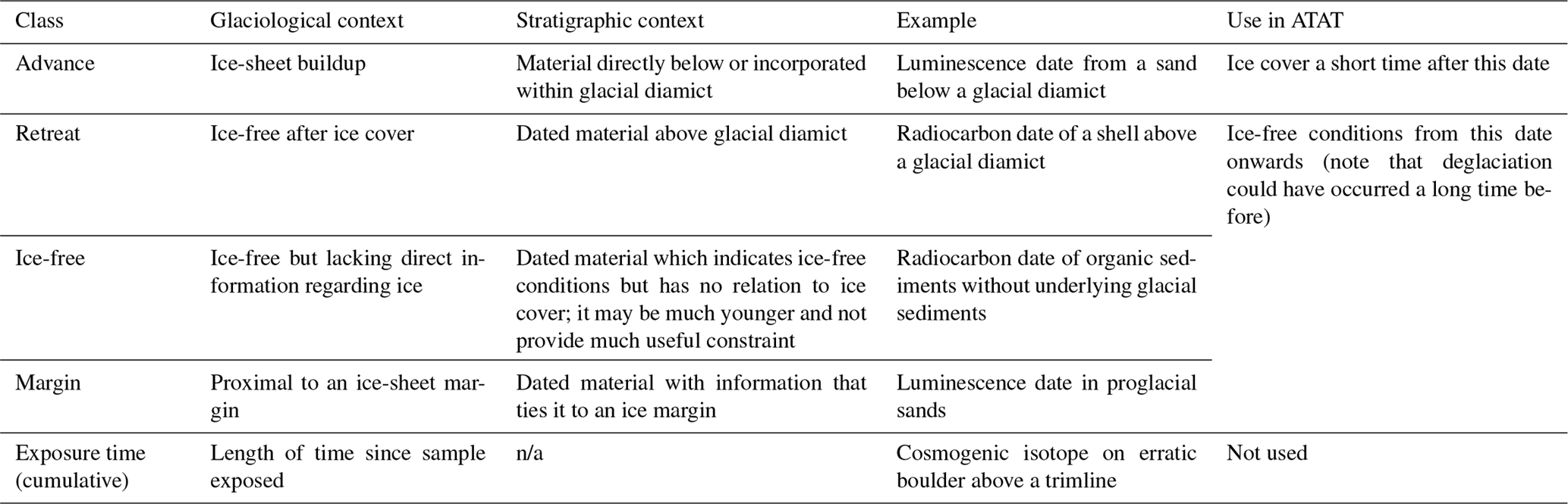
The timing of palaeo-ice-sheet activity has primarily been dated using three techniques: (i) radiocarbon dating, (ii) cosmogenic nuclide exposure dating and (iii) luminescence dating (Fig. 1). The utility of each method for determining the timing of palaeo-ice-sheet activity has been extensively reviewed elsewhere (e.g. Fuchs and Owen, 2008; Balco, 2011; Small et al., 2017) and only a brief description is provided here. Radiocarbon dating uses the known rate of the radioactive decay of 14C to determine the time elapsed since the death of organic material (Libby et al., 1949; Arnold and Libby, 1951; Fig. 1). For palaeo-glaciological purposes, the dated organic material (e.g. shells, mosses, plant remains) is usually taken from basal sediments overlying and closely associated with a glacial deposit in order to determine a minimum deglaciation age (e.g. Heroy and Anderson, 2007; Lowell et al., 2009); ice is interpreted to have retreated from this site some short time prior to this age. Where organic matter is either reworked within or is located directly beneath a glacial deposit, it can be used to constrain the maximum age of glacial advance (e.g. Brown et al., 2007; Ó Cofaigh and Evans, 2007); advance happened sometime after this age. Cosmogenic nuclides (e.g. 10Be, 26Al and 36Cl) are produced by the interaction of secondary cosmic radiation in minerals, such as quartz, within materials exposed at the Earth's surface (Fig. 1). Samples are generally taken from glacially transported boulders, morainic boulders and glacially modified bedrock, all of which have ideally had signals from any previous exposure history removed by glacial erosion. Cosmogenic nuclide dating is thus used to determine the duration of time a sample has been exposed at the Earth's surface by determination of the concentration of cosmogenic nuclides within that sample. Luminescence dating can determine the age of a deposit by measuring the charge accumulated within minerals. This charge accumulates in light-sensitive traps within the crystal lattice due to ionising radiation produced by naturally occurring radioactive elements (e.g. U, Th, K). Luminescence dating determines the time elapsed since the last exposure of the mineral to sunlight; this exposure acts to reset the signal (Fig. 1). As subglacial deposits are unlikely to have been exposed to light before burial and therefore contain signals accumulated prior to deposition, luminescence dating within palaeo-glaciology is typically applied to ice-marginal sediments or those which overly glacial sediments (e.g. Duller, 2006; Smedley et al., 2016; Bateman et al., 2018). All geochronological techniques record the absence of grounded ice. They therefore provide either maximum or minimum ages of a glaciological event, depending upon the stratigraphic setting. Table 1 outlines a commonly used system used to classify geochronological data by stratigraphic setting (Hughes et al., 2011, 2016).
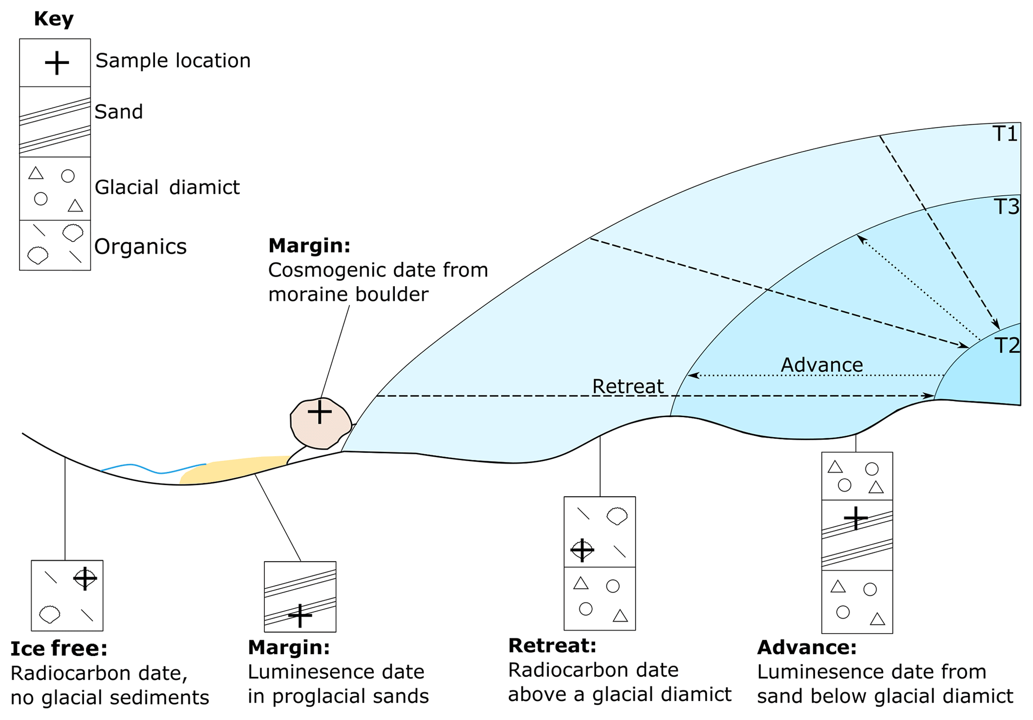
Figure 1Schematic illustration of stratigraphic and inferred glaciological context of geochronological data. Note that at T1 the ice sheet is at its most advanced. It then retreats to a minimum at T2, before readvancing to T3.
Table 1Classification of geochronological data (after Hughes et al., 2011) and their use in ATAT. “n/a” means “not applicable”.
The retreat/advance (ice-free) ages provided by the three geochronometric techniques are all affected by systematic and geological uncertainties (Small et al., 2017). Systematic uncertainties originate from the tools and techniques used to derive the date, such as laboratory instruments and sample preparation, and are accounted for in the quoted errors that accompany a date. Geological uncertainties are caused by the geological history of a sample before, during and after a glacial event (e.g. Lowe and Walker, 2000; Lukas et al., 2007; Heyman et al., 2011). Such influences may leave little or no evidence of their effect upon a sample and are thus hard to quantify. The relationship between a dated sample and the glacial event it indicates is the largest potential source of uncertainty in geochronological data and is primarily bounded by the ability of the investigator to find and associate dateable material to the glacial event of interest. Since all geochronological techniques measure the absence of ice, expert inferences must be made and are influenced by the availability of information (stratigraphic or otherwise) at a study site; they may be open to change (e.g. new radiocarbon calibrations, new cosmogenic isotope production rates). Furthermore, in the cases of luminescence and radiocarbon dating, there can be an unknown duration since the glacial occupation of an area and the deposition of dateable material. These factors mean it is necessary to consider the quality of dates for ascertaining the timing of the glacial event in question (Small et al., 2017).
Numerous geochronological studies have sought to ascertain the timing of palaeo-ice-sheet activity at sites, leading to compilations of geochronological data which bring together hundreds to thousands of published dates (e.g. Dyke, 2004; Livingstone et al., 2012; Hughes et al., 2011, 2016). Despite the growing number of reported dates, they are still insufficient in number and spatial spread to define, on their own, the time–space envelope of the shrinking ice sheet. Techniques to interpolate geochronological information between sites are required. The most commonly used technique is empirical ice-sheet reconstruction (e.g. Dyke, 2004; Clark et al., 2012), whereby expert assessments of the geochronological and geomorphological record are used together to create ice-sheet-wide isochrones of ice-sheet margin position and flow configuration. A recent advance in this method has been the inclusion of confidence envelopes for each isochrone, documenting possible maximum, likely and minimum extents (Hughes et al., 2016). Further techniques for spatiotemporally interpolating geochronological data include Bayesian sequence modelling (e.g. Chiverrell et al., 2013; Smedley et al., 2017), in which collections of deglacial ages are arranged in spatial order determined by a priori knowledge of geomorphologically informed ice-flow and retreat patterns (e.g. Gowan, 2013). Such techniques provide viable methods for producing ice-sheet-wide chronologies, filling in information in locations where geochronological data may be sparse.
2.2 Ice-sheet model output
Ice-sheet models solve equations for ice flow over a computational domain, for a given set of input parameters and boundary conditions, to determine the likely flow geometry and extent of an ice sheet. Typically, ice-sheet models run using finite difference techniques on regular grids (e.g. Rutt et al., 2009; Winkelmann et al., 2011). Ice-sheet models that utilise adaptive meshes (e.g. Cornford et al., 2013) and unstructured meshes also exist (e.g. Larour et al., 2012) and the results from such models can be interpolated onto spatially regular grids. The spatial resolution of an ice-sheet model depends upon the computational resources available and the spatial resolution of available boundary conditions. Continental-scale models of palaeo-ice sheets have typical spatial resolution of tens of kilometres (e.g. Briggs and Tarasov, 2013; DeConto and Pollard, 2016; Patton et al., 2016), though parallel, high-performance computing means higher resolutions are possible (e.g. 5 km in Golledge et al., 2013; Seguinot et al., 2016). The temporal resolution of ice-sheet model output is ultimately limited by the time steps imposed by the stability properties of the numerical schemes solving the ice-flow equations. Given that these stable time steps can be sub-annual, output frequency is mostly predetermined by the user (typically decades to centuries) and as such is constrained by available disk storage. Ice-sheet models therefore produce spatially connected predictions of ice-sheet behaviour such as advance and deglaciation (e.g. Table 1) across gridded domains at various temporal and spatial resolutions.
The stress fields imposed upon ice can be fully described by solving the Stokes equations. Indeed, “full Stokes” models which do so have been tested (Pattyn et al., 2008) and used to simulate ice sheets (e.g. Seddik et al., 2012). However, fully solving the Stokes equations over the spatiotemporal scales relevant to palaeo-ice-sheet researchers remains beyond the limit of currently available computational power. This problem is exacerbated by the need to run multi-parameter-valued ensemble simulations to account for model uncertainty over multi-millennial and continental-scale domains. This means that palaeo-ice-sheet modelling experiments rely upon approximations of the Stokes equations (see Kirchner et al., 2011 for a discussion), such as the shallow ice approximation (SIA) and shallow shelf approximation (SSA). The choice of ice-flow approximation used within a model has implications for the capability of models to realistically capture aspects of ice-sheet flow (Hindmarsh, 2009; Kirchner et al., 2011, 2016) and in turn influences the nature of the model output produced. For instance, the SIA is not applicable for ice shelves; therefore, SIA-based models do not produce modelled ice shelves (e.g. Glimmer; Rutt et al., 2009). Therefore, the timing of deglaciation in a SIA model can be determined as the point at which ice thickness in a cell becomes zero or thinner than the flotation thickness, whereas in a SSA or higher-order model the location and movement of the grounding line must be determined.
Though ice-sheet models produce output which is consistent with model physics, like all numerical models of physical systems (e.g. Rougier, 2007), there are many sources of uncertainty involved with ice-sheet modelling. Three broad sources of model-based uncertainty can be distinguished: (i) downscaling; (ii) parametric uncertainty; (iii) structural uncertainty. These are defined and discussed below.
Downscaling uncertainties arise due to an ice-sheet model's computation over space which has a coarser resolution than reality. This means that a characteristic which can be measured to a high level of accuracy and precision for a real ice sheet (e.g. the position of a calving front) has a larger uncertainty in an ice-sheet model. This is especially pertinent for data–model comparisons, as most observations of ice-sheet activity have a sub-model resolution.
Parametric uncertainty has two main sources: (i) parameterisations and (ii) boundary conditions. Where a process is too complex (e.g. calving) or occurs at too small a scale (e.g. regelation) to be captured by an ice-sheet model, it is often simplified and parameterised. Associated with each parameterisation is a set of parameters, the values of which are either unknown or thought to vary within some plausible bounds, and which can either be constant or spatially and temporally variable across a domain. An example of a process which is often parameterised is basal sliding. This parameterisation is often done through the implementation of a sliding law (e.g. Fowler, 1986; Bueler and Brown, 2009; Schoof, 2010), which relates the basal shear stress to the basal velocity (Fowler, 1986). Parameters used to determine this relationship are often assigned or incorporated within a parameter, or prescribed by another model parameterisation (e.g. a subglacial hydrology model). Adding to the uncertainty in the absence of a single preferable sliding law, ice-sheet models often allow the user to choose between different sliding law implementations.
Boundary conditions, the values prescribed at the edge of the modelled domain, also introduce uncertainty into ice-sheet models. For contemporary ice sheets, there is a large uncertainty in the basal topography (e.g. Fretwell et al., 2013). This is less of a problem for the more accessible beds of palaeo-ice sheets. However, accurately accounting for the evolution of this bed topography over the course of a glaciation requires a model of isostatic adjustment (Lingle and Clark, 1985; Gomez et al., 2013).
A very large source of uncertainty for modelling palaeo-ice sheets is the climate used to drive them (Stokes et al., 2015), as indeed is the case for forecasts of contemporary ice sheets (e.g. Edwards et al., 2014). Due to the computational resources required and technical challenges, few palaeo-ice-sheet models are coupled with climate models. This uncertainty over past climate is reflected in the large range of outputs produced by global circulation models which have tried to simulate the last glacial cycle (e.g. Braconnot et al., 2012). Palaeo-ice-sheet modellers have used a range of methods to force their models, including simple parameterisations (Boulton and Hagdorn, 2006), applying offsets derived from ice-core records to contemporary climate (e.g. Huybrechts, 1990; Hubbard et al., 2009) and scaling between present-day conditions and uncoupled global-circulation-model simulations at maximum glacial conditions (e.g. Greve et al., 1999; Gregoire et al., 2012; Gasson et al., 2016). Each approach is associated with an inherent uncertainty. When this uncertainty is accounted for in an ensemble experiment, the range of possible climates produces numerous ice-sheet outputs.
Structural uncertainty is related to parametric uncertainty, but has a broader remit, and is defined as uncertainty which occurs due to differences in model coding and design (Collins, 2007; Tebaldi and Knutti, 2007). This encompasses differences in which processes are included in different models and also the manner in which they are implemented. Structural uncertainty is difficult to quantify but can be explored by multi-model comparison (Murphy et al., 2004; Collins et al., 2011). Such comparisons are not currently routine in palaeo-ice-sheet modelling. Differences in model coding (i.e. structural uncertainty) arise due to a lack of understanding regarding the physical system in question. This points to a broader uncertainty with a similar remit that no models can include processes that are as yet unknown to science. Reducing this source of uncertainty is an ongoing challenge for glaciology.
There is another uncertainty which hinders ice-sheet models from being able to accurately predict the evolution of ice sheets, which is the presence of instabilities – we use this term in the technical sense of a small perturbation that leads to the whole ice-sheet system amplifying this small perturbation to the extent it can leave a mark in the geological record. A classic example of this in ice-sheet dynamics is the marine ice-sheet instability (MISI), first discussed in the 1970s (Hughes, 1973; Weertman, 1974; Mercer, 1978) and more recently put on a sounder mathematical footing (Schoof, 2007, 2012).
The MISI actually refers to an instability in grounding-line (GL) position on a reverse slope, where the water depth is shallowing in the direction of ice flow. Since ice flux increases with ice thickness, a straightforward argument leads to the conclusion that if the GL advances into shallower water, the efflux will decrease, the ice sheet will gain mass and the advance continue. If, on the other hand, the GL retreats, the flux will increase, the ice sheet will lose mass and the retreat continue. In principle, given the right parameterisations and basal topography, ice-sheet models should be able to predict the “trajectory” of GL migration arising as a consequence of the MISI. However, the MISI is one of the class of instabilities that lead to poor predictability; certain small variations of parameters and specifications will lead to large-scale changes in the “trajectory”, in this case the retreat history. A well-known analogy is the “butterfly effect”, which originated in atmospheric modelling work (Lorenz, 1963); the butterfly effect is concerned with the consequences of the statement “small causes can have larger effects”. Recent work has also shown that additional physical processes, such as ice-shelf buttressing (Gudmundsson, 2013) and the effect that the gravitational pull of ice sheets has on sea level (Gomez et al., 2012), have additional effects on grounding-line stability. Given that most of the palaeo-ice sheets during the last glacial cycle had extensive marine margins and over-deepened basins, with isostatic adjustment creating further zones of reverse slope, capturing grounding-line processes is important for simulating these ice sheets.
2.3 Considerations when comparing geochronological data and ice-sheet model output
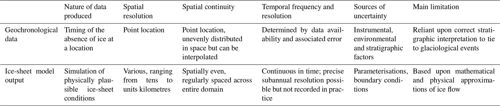
Section 2.1 and 2.2 make it clear that several factors must be considered in order to satisfactorily compare geochronological data and ice-sheet model output (Table 2). Most critically, the two datasets involved in any comparison have varying spatial properties. Raw geochronological data are unevenly distributed and located at specific points, with horizontal position accurate to a metre or so; such data may be used to plot ice-margin fluctuations of the order of tens of kilometres (Fig. 2c). Ice-sheet models typically produce results on evenly spaced points (at ∼5 to 20 km resolution) that are distributed over and beyond the maximum area of the palaeo-ice sheet (Table 2; Fig. 2b). Consequently, in comparing the two, a choice must be made; either geochronological data should be gridded (coarsened) to the resolution of the ice-sheet model, or the ice-sheet model results must be interpolated to a higher resolution. Both options have drawbacks, as the former removes spatial accuracy from geochronological data, while the latter relies upon interpolation beyond model resolution and, more seriously, model physics. A second problem lies in the spatial organisation of the data (Table 2). Ice-sheet models produce a regular grid of data (Fig. 2b), meaning that no location is more significant than any other when comparing the modelled deglacial chronology with that inferred from geological data. Conversely, due to the uneven distribution of raw geochronological data, some regions of a palaeo-ice sheet may be better constrained than others (Fig. 2c). As noted by Briggs and Tarasov (2013), any comparison that does not treat the uneven spatial distribution of geochronological data may favour sites where numerous dates exist over more isolated locations. One approach to overcoming these disparities is to use an interpolation scheme (e.g. empirical reconstruction, Bayesian sequence) on the raw geochronological data. This produces a geochronological framework by combining evidence on pattern and timing to yield a distribution that is spatially more uniform and a spatial resolution similar to that of palaeo-ice-sheet model output (Fig. 2d).

Figure 2Schematic of geochronological data and ice-sheet model output. (a) A deglaciated landscape, demonstrating some of the features used by palaeo-glaciologists when empirically reconstructing an ice sheet. (b) Ice-sheet model output, displaying modelled ice-sheet thickness, in this case at a specific time. (c) Geochronological data. (d) Empirical reconstruction. Note how the nature of these data varies between sources.
Table 2Comparison of attributes between geochronological data and ice-sheet model output.
The temporal intervals between and precision of geochronological data and ice-sheet model output also vary (Table 2). The time intervals between geochronometric data are determined by the number of available observations and precision determined by sources of uncertainty. Conversely, ice-sheet models produce output at regular intervals and are temporally exact, which is to be contrasted with “correct”. Since the output interval of an ice-sheet model is generally determined by the user (see Sect. 2.2), it is pertinent to consider an appropriate time interval of ice-sheet model output for comparison with geochronological data. For example, radiocarbon dates have precision typically on the order of hundreds of years but do not directly constrain ice extent, whilst empirically reconstructed isochrones are typically produced for 1000-year time slices (e.g. Hughes et al., 2016). In reality, ice sheets may respond to events at faster timescales than this but in the absence of internal instabilities (e.g. MISI) palaeo-ice-sheet models are ultimately limited by the temporal resolution of the available climate forcing data. Thus, to gain insight into controls on palaeo-ice-sheet behaviour, it may be necessary to create model output with a greater (centurial) temporal resolution than the uncertainty associated with geochronology.
Both geochronological data and ice-sheet model output have sources of uncertainty which must also be considered when comparing the two. For geochronological data, uncertainty is typically expressed as a standard deviation from the reported age and is therefore easy to consider when comparing to an ice-sheet model. For ice-sheet models, individual model runs do not currently express uncertainty, and it is only when multiple (ensemble) runs which systematically vary parameters and boundary conditions are conducted that uncertainty in all output variables can be expressed. Therefore, any comparison between geochronological data and model simulations must either compare to all members of an ensemble experiment in turn or against amalgamated output from an ensemble which considers model uncertainty. Having said this, statistical techniques exist to derive probability distribution functions for individual quantities (e.g. Ritz et al., 2015). Such ensemble runs typical comprise hundreds to thousands of individual runs (Tarasov and Peltier, 2004; Robinson et al., 2011). Given the volume of data this produces, one appealing application of a quantitative comparison between geochronological data and ice-sheet model output would be to act as a filter for scoring ice-sheet model runs and reducing predictive uncertainty by only using the parameter combinations that were successful. However, if all possible parameters have been modelled (i.e. the full “phase-space” of the model has been explored (see Briggs and Tarasov, 2013)), and very few (or no) model runs conform to a certain set of geochronological data or an empirical reconstruction, this may provide a basis to question aspects of the evidence (e.g. re-examining the stratigraphic context of a dated sample site or questioning the basis of the reconstructed isochrone). Of course, a third possibility that both data and model are incorrect cannot be excluded.
We therefore suggest that any comparison between ice-sheet model experiments and geochronological data should consider the following:
- (i)
Both ice-sheet models and geochronological data have inherent uncertainties.
- (ii)
Geochronological data typically provide a constraint on just the absence of ice, such that ice must have withdrawn from a site sometime (50 years? 500 years? 5000 years?) prior to the date (which can be any point within the full range of the stated uncertainty). It is thus a limit in time and not a direct measure of glacial activity. Figure 3 illustrates this for advance and retreat constraints. It is most often the case that dated material is taken close to the stratigraphic boundary or landform representing ice presence, in which case a date might be considered as a “tight constraint” (e.g. the ice withdrew and very soon afterwards (50 years) marine fauna colonised the area and deposited the shells used in dating). Sometimes, however, there may have been a large (centuries to millennia) interval of time between the withdrawal and the age of the shell chosen as a sample, in which case the date will provide a “loose” limiting constraint; it might be much younger than ice retreat (Fig. 3).
- (iii)
There is inherent value to the expert interpretation of stratigraphic and geomorphological information, meaning an ice-free age reported for a site is likely as close as possible (tight constraint) to a glacial event. However, this interpretation could be subject to change.
- (iv)
Geochronological data exist as spatially distributed dated sites (e.g. Fig. 2c) which can be built into a spatially coherent reconstruction (e.g. Fig. 2d).
- (v)
A great input uncertainty in a palaeo-ice-sheet model is the climate, which can lead to changes in the spatial extent and timing of ice-sheet activity.
- (vi)
A factor which requires further investigation is the relationship between the operation of a physical instability (e.g. MISI) and the practical ability of models to predict retreat or advance rates; the presence of an instability can result in extreme sensitivity to parameter ignorance or oversimplified model physics.
- (vii)
Other uncertainties can also lead to variations in ice-sheet model results; these can be accounted for in an ensemble of hundreds to thousands of simulations.
Given the above, it is unlikely that a single procedure could capture model–data conformity. ATAT therefore implements several ways of measuring data–model discrepancies and produces output maps (described in the following two sections) to help a user assess which model runs best agree with the available geochronological data. One approach is to transform the geochronological data points (x, y, t) to a gridded field (raster) that defines age constraints of ice advance and another grid for retreat. Both of these data types also require an associated grid that reports the uncertainty range as error (Fig. 4). These age grids may then be quantitatively compared to equivalent grids (age of advance grid and age of retreat grid) derived from the ice-sheet model outputs. Alternatively, one might prefer to compare model runs against the geochronological data (points) combined with expert-sourced interpretive geomorphological and geological data, in which age constraints from dated sites have been spatially extrapolated using moraines and the wider retreat pattern. In this case, ATAT allows the model outputs to be compared to the “lines on maps” type of reconstruction subsequent to conversion from age isolines to a grid of ages (Fig. 4).
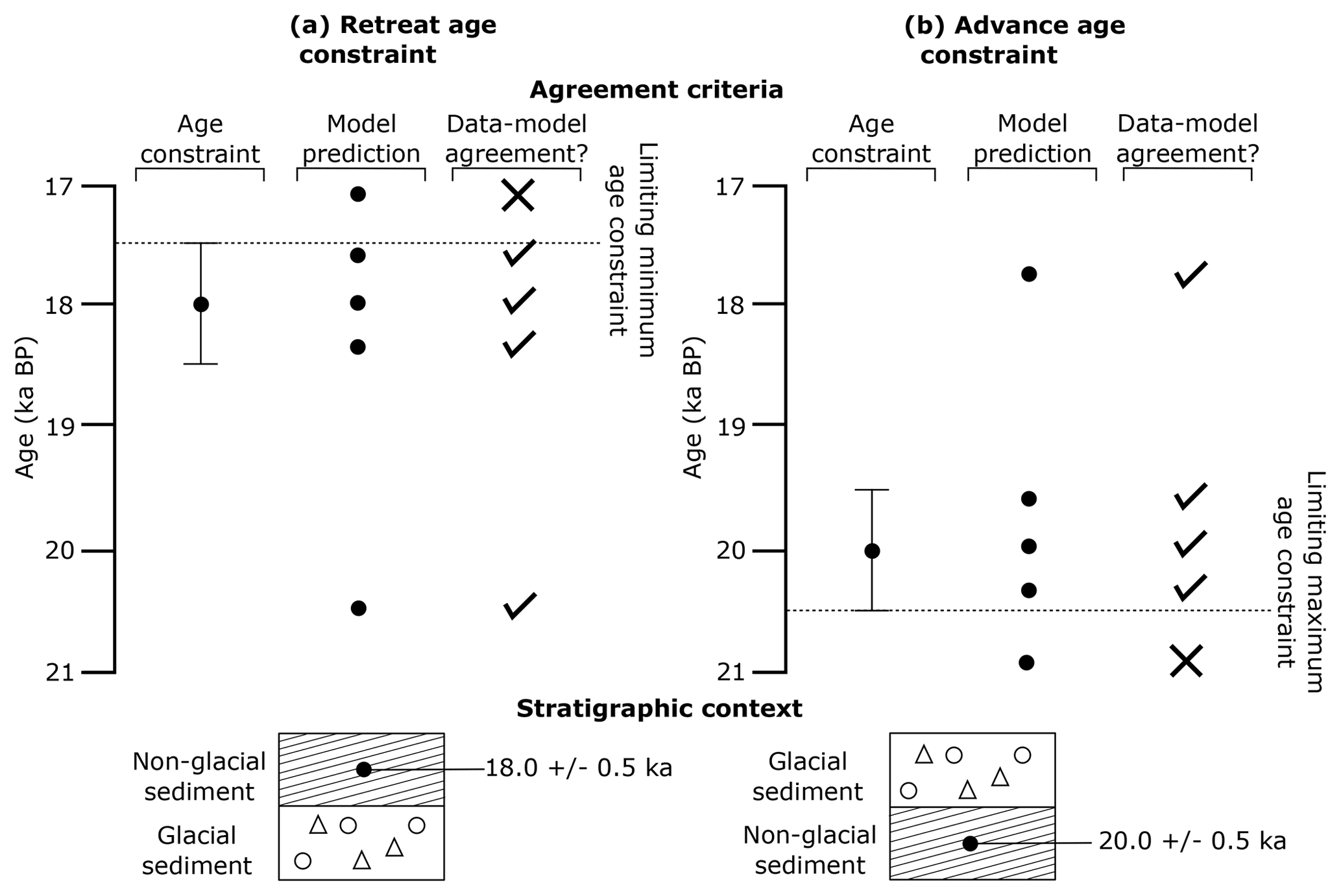
Figure 3Schematic of the identification of data–model agreement with consideration of error by ATAT for retreat (a) and advance (b) data. If a model predicts ice-free conditions before an ice-free age, or during the associated error, there is data–model agreement. If deglaciation occurs at this location after the error, the model disagrees with the data. If a model predicts ice advance and cover before the advance age and its associated error, there is model–data disagreement. Agreement between the model and data occurs if ice advances over the location after the date or before the date within the range of the error. This is used by ATAT to categorise sites as to whether agreement or disagreement between the model and data occurs.
ATAT is written in Python and utilises several freely available modules. Access to these modules may require a Python package manager, such as “pip” or “anaconda”. ATAT can therefore be run from the command line on any operating system, or by using a Python interface such as IDLE.
3.1 Required data and processing
ATAT requires two datasets as an input: (i) an ice-sheet model output and (ii) gridded geochronological data. Table 3 provides the required variables and standard names for each dataset. In order to determine the advance age or deglacial age predicted by the ice-sheet model, ATAT requires either an ice thickness (where the model does not produce ice shelves) or a grounded ice-mask variable (where ice shelves are modelled). In the latter case, the user is asked to define the value which represents grounded ice.

Empirical advance and deglacial geochronological data (Table 1) require separate input files (NetCDF format), as model–data comparisons for these two scenarios are run separately in ATAT. Table 1 and further references (Hughes et al., 2011, 2016; Small et al., 2017) provide information regarding identification of the stratigraphic setting of these two glaciological events as considered by ATAT. ATAT requires that geochronological data (advance or deglacial) are interpolated onto the same grid projection and resolution as the ice-sheet model before use. Though an imperfect solution to the problem of comparing grids of different resolution (Sect. 2.3; Table 2), this was preferred to the alternative solution of regridding an ice-sheet model onto a higher-resolution grid, as this may introduce the false impression of high-resolution modelling sensitive to boundary conditions (e.g. topography) beyond the actual model resolution.
Preparation of the geochronological data to be the same format and grid resolution as the ice-sheet model output requires use of a GIS software package such as ESRI ArcMap or QGIS. Users must define deglacial/advance ages based either upon the availability of geochronological data in a cell or based upon an empirical reconstruction (Fig. 4). These ages must be calibrated to a calendar which is the same as that output by the ice-sheet model (in our case the 365-day calendar in units of seconds since 1–1–1). Where there are no data (i.e. outside the ice-sheet limit), the grid value must be kept at 0. When multiple dates are contained within a cell, expert judgement is required to ascertain which date is most representative of the deglaciation of a region. This assessment should be based upon the quality of sample taken; criteria for establishing this quality are considered in Small et al. (2017). In the case where a profile of dates has been collected (for example, up a vertical section at the side of a valley, or from multiple depths of a marine core), the date which most closely defines the timing of final deglaciation of an area should be chosen, as this is the focus of ATAT. The assembly of this geochronological database input into ATAT should consider the reliability of ages, removing outliers and unreliable ages (see Small et al., 2017 for a discussion of this issue). In particular, loose constraints, such as cosmogenic dates which display inheritance or radiocarbon dates effected by a depositional hiatus, should be removed, as these have the potential to bias results. In a comparable manner, the attribution of error to each cell is also reliant upon expert interpretation. The magnitude of error may vary between the source of geochronological data (radiocarbon, cosmogenic nuclide or luminescence) and user choice for experimental design (e.g. 1, 2 or 3σ). A single error value must be given for each dated cell, corresponding to the maximum threshold beyond which the user deems it is unacceptable for a model prediction to occur (Fig. 3). Given that creating these input data may involve many expert decisions (e.g. which date has the relevant stratigraphic setting, which date(s) are most reliable), this part of the process is not yet automated within ATAT. This data preparation stage is therefore the most time-consuming and user-intensive part of the process. However, users only need to define the data-based advance/deglacial grid once to compare to multiple model outputs. Future work should consider alternatives means of choosing dates and identifying outliers, such as Bayesian age modelling (e.g. Chiverrell et al., 2013). The input data NetCDF file should also contain the variables' latitude, longitude, base topography (the topography that the ice-sheet modelling is conducted on) and the elevation of the geochronological sample (Table 3).
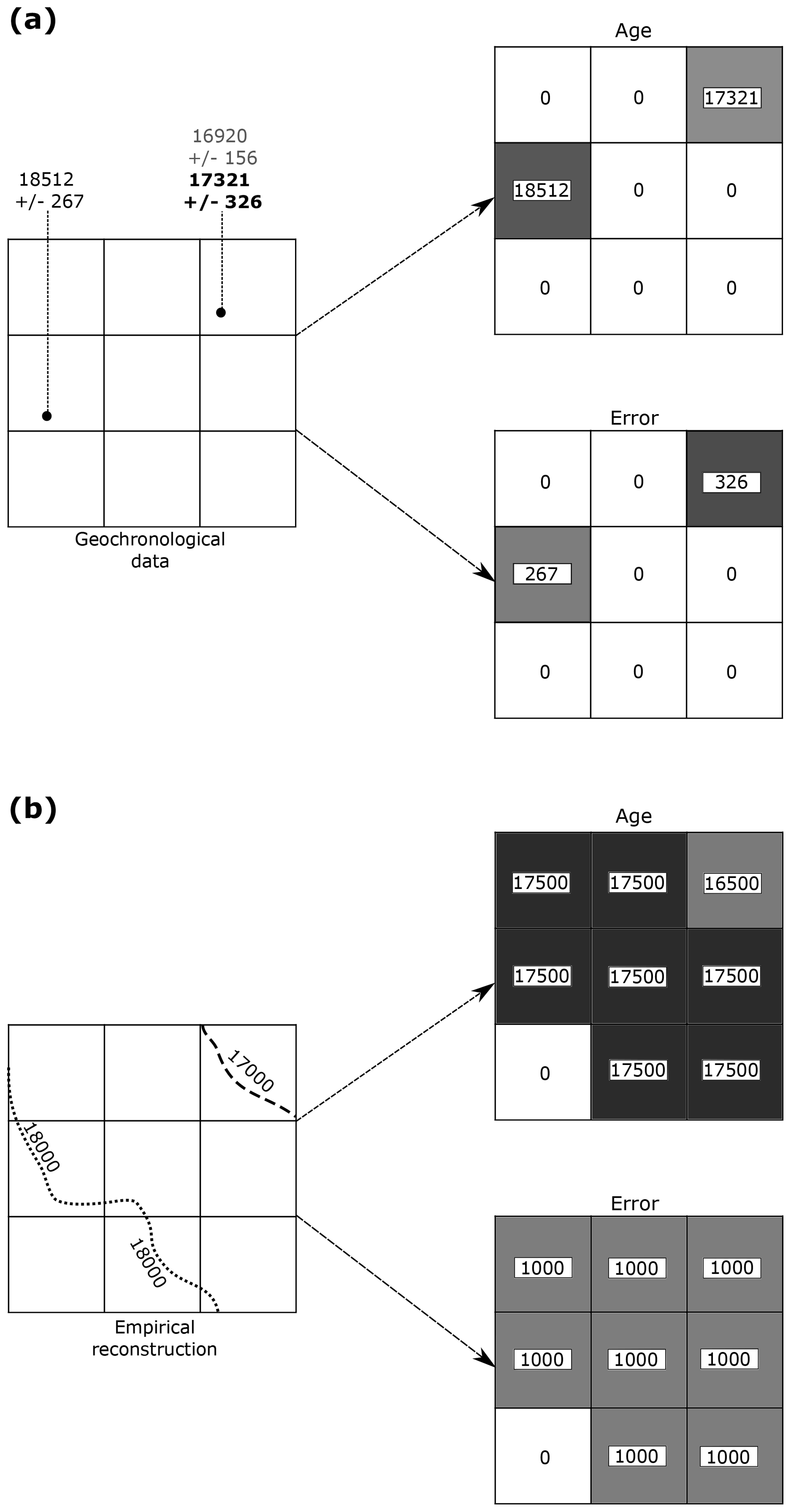
Figure 4Examples of empirical data preparation for ATAT. (a) Conversion of geochronological data into a grid for ATAT. In this example, the user has made a judgement based on a priori knowledge that the date of 17 321±326 is most representative of the event of interest. Note that age and error are split into separate grids and that no data regions are assigned a value of 0. (b) Conversion of an empirical reconstruction (margin isochrones) into a grid for ATAT. Here, we simply assume that the area between isochrones became deglaciated at the age between the two isochrones and that associated error is 1000 years. More complex reconstructions (e.g. Hughes et al., 2016) may require different user-defined rules.
ATAT is called from a suitable Python command-line environment, using several system arguments to define input variables (Table 1; Fig. 5). Users must define whether they are testing a deglacial or advance scenario. ATAT only considers the last time that ice advanced over an area. Therefore, caution must be undertaken when defining advance data in regions where multiple readvances occur, and users should consider limiting the time interval of the ice-sheet model tested when examining specific events (e.g. a well-dated readvance or ice-sheet buildup). The location of the file containing the geochronological data grid (e.g. Fig. 5) is then required. From this file, the age and error grids are converted to arrays. For the age data, null values are masked out using NumPy's masked array function. A second array that accounts for error is then created, the properties of which depend upon whether a deglacial or advance scenario is being tested. For a deglacial scenario, a model prediction will be unacceptable if the cell is ice covered after the range of the date error is accounted for, but the cell may become deglaciated any time before this. Therefore, the associated error value is added onto the cell date to create a maximum age at which a cell must be deglaciated by to conform to the ice-sheet model (Fig. 3). The opposite is true for advance ages; ice can cover a cell any time after the date and associated error but cannot cover the cell before the date of the advance. In order to allow for advances which occur after the date and its error, associated error is therefore subtracted from the date cell (Fig. 3). To account for the uneven spatial distribution of dates, a weighting for each date is then calculated based upon their spatial proximity. This weighting is used later when comparing the data to the model output. To calculate this weighting (wi), ATAT defines a local spatial density of dated values based upon a kernel search of 10 neighbouring cells.
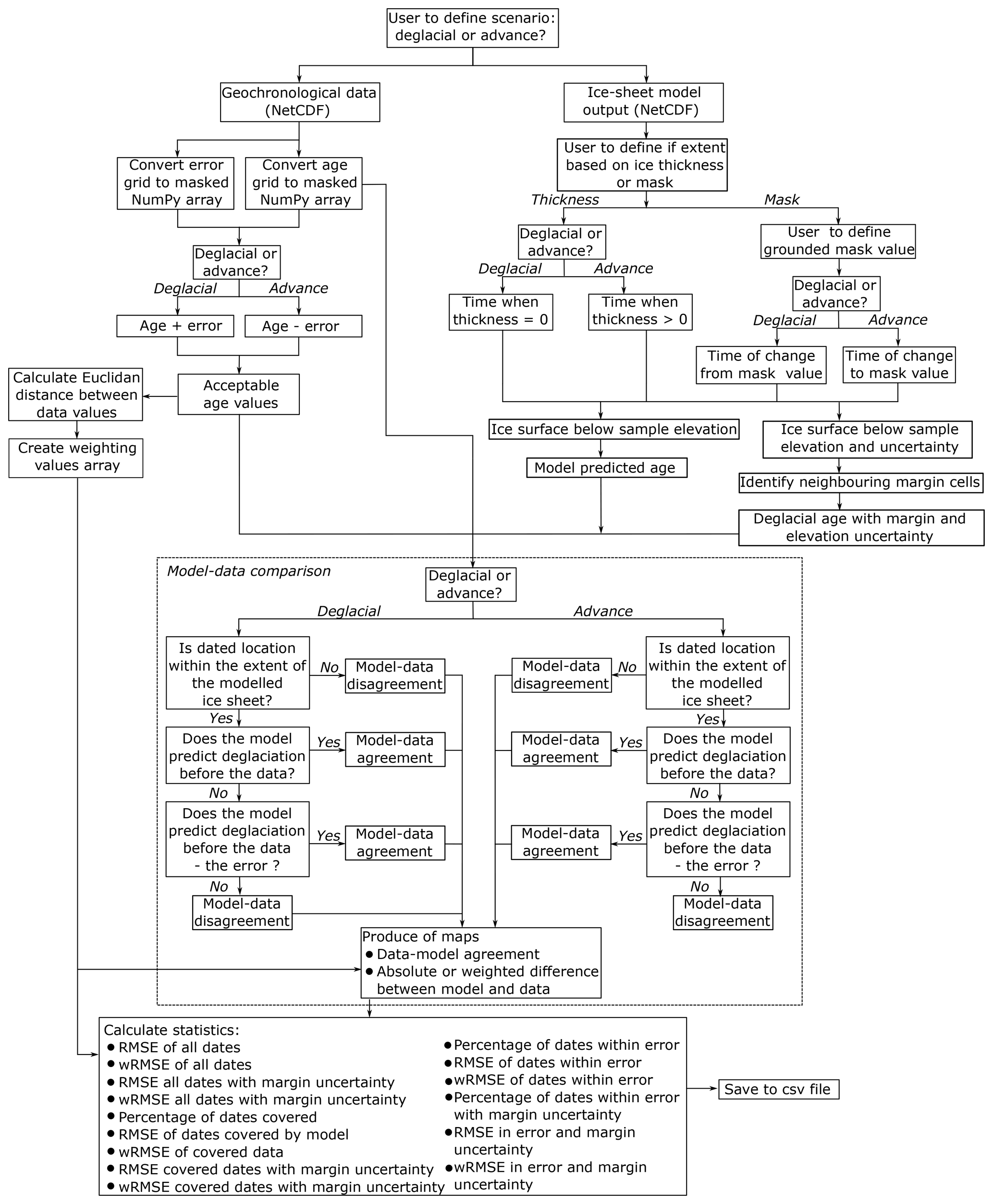
The user must define the path to the ice-sheet model output, from which the modelled deglacial age will be calculated and eventually compared to the data (Fig. 4). The user must also define whether to base deglacial timing on an ice thickness or grounded extent mask variable (Table 2). If the user selects thickness, the margin is defined by an increase from 0 ice thickness. For the mask, the user is also asked to supply the number which refers to grounded ice extent. The timing of advance is then determined by the change of a cell to this number (Fig. 5). The margin position recreated by the ice-sheet model has a spatial uncertainty due to downscaling issues and fluctuations which may occur between recorded outputs. To account for this, ATAT calculates a second set of modelled deglacial ages, whereby the deglaciated region at each modelled time output is expanded to all cells which neighbour the originally identified deglaciated or advanced over cells. Furthermore, the spatial resolution of ice-sheet models typically means that the emergence of ice-free topography at the edge or within an ice-sheet (e.g. in situations such as steep-sided valleys or nunataks) is poorly represented. To account for this, ATAT firstly calculates the modelled ice-sheet surface at each time output by adding ice thickness to the input base topography. Where the modelled surface elevation is below that of the sample elevation, these cells are identified as being deglaciated (Fig. 5). The downscaling of topography onto ice-sheet model grids also introduces a vertical uncertainty. This is accounted for in ATAT through calculating the difference between sample elevation and the reference elevation. A second metric which identifies cells as having been deglaciated if they are also within this vertical uncertainty is also calculated (Fig. 5).
3.2 Model–data comparison
Once the required variables have been retrieved from the NetCDF data and manipulated, ATAT compares the geochronological age and modelled age at each location (Fig. 4). Firstly, the grid cells which have data are categorised as to whether there is model–data agreement, based on the criteria shown in Fig. 3. Since all dating techniques only record the absence of ice, geochronological data provide only a one-way constraint on palaeo-ice-sheet activity. For deglacial ages, deglaciation could occur any time before the geochronological data provided and within the error of the date (i.e. deglacial ages are minimum constraints), but deglaciation must not occur after the error of the date is considered (Fig. 3). For advance ages, advance must have happened after the date or within error beforehand (i.e. advance ages are maximum constraints), but palaeo-ice-sheet advance cannot occur in the time period before that dated error (Fig. 3). Once ATAT has determined whether each cell conforms to these criteria, a map is produced identifying at which locations the ice-sheet model agrees with the geochronological data.
Though the criteria described above and illustrated in Fig. 3 allow for the identification of dates which conform to the predictions of an ice-sheet model, they provide little insight into how close the timing of the model prediction is to the geochronological data. If these were the only criteria on which a model–data comparison was made, it could prove problematic. In an extreme case, one could envisage that all retreat dates are adhered to by a model run that deglaciates from a maximum extent implausibly rapidly (say 50 years!), and given that we only have one-way (minimum) constraints on deglaciation (Fig. 3), this model run would conform to all modelled dates. Whilst the nature of geochronological data (being only able to determine the absence of ice) does not preclude such a scenario, this assumes that there is no inherent value to the expert judgement and stratigraphic interpretation of each date as being close to palaeo-ice-sheet timing (see Small et al., 2017). Therefore, ATAT also determines the temporal proximity of the geochronological data and the model prediction. Firstly, a map of the difference between modelled and empirical ages is created (Fig. 5). This enables the identification of dates which are a large distance away from the model prediction. Secondly, the root mean square error (RMSE) is calculated using Eq. (1):
where n is the number of cells which contain empirical geochronological information, gi is the associated geochronological date, and mi is the model-predicted age. The RMSE works well when the geochronological data are evenly spatially distributed, either from a reconstruction (i.e. isochrones) or a wealth of dates. ATAT also calculates a weighted RMSE (wRMSE), for situations where this is not the case (i.e. there is a paucity of dates that are not distributed evenly across the domain) using Eq. (2):
where wi is the spatial weighting factor. Results of the RMSE and wRMSE calculations are separated by the degree to which included dates agree with model output. This creates an array of metrics with varying levels of consideration of model and data uncertainty (Fig. 5). Both the RMSE and wRMSE are calculated for all dates to create a metric that does not account for dating error but may give an indication of how close a model run gets to dated cells. Dated locations are also categorised according to whether model–data agreement occurs within dating error, and whether the addition of horizontal (ice-margin) and vertical (ice-surface) downscaling uncertainty means that model–data agreement occurs. The RMSE and wRMSE are calculated for these categories to create a metric which accounts for data and model uncertainty (Fig. 5). ATAT then produces a .csv file containing all calculated statistics per ice-sheet model output file. We suggest that the most rigorous metric, the wRMSE of dates which conform within geochronological data and model downscaling uncertainty (Fig. 5), should most frequently used. However, other metrics, such as the RMSE of all dates, may give an indication of performance earlier in the modelling process. For example, initial results may reveal that no or very few dates conform to a set of model simulations within model and data uncertainty, but the RMSE of all dates may give an indication of models and associated parameters to be explored further. Given the complexity of data–model comparison, different statistics may have different uses. For instance, the percentage of covered dates may prove useful to identify the worst-performing model runs (i.e. the bottom 50 %), whilst the wRMSE of dates within error may be more convenient for choosing between model runs. However, given the uncertainty in ice-sheet modelling, it is likely that in an ensemble there will be no single model run which has significantly better metrics than others, so ATAT may best be used to choose members which pass a user-defined threshold of combined metrics.
Pragmatically, we envisage that ATAT could be used in the following ways, though others may exist. In sensitivity experiments (e.g. Huybrechts, 1990; Hubbard et al., 2009; Patton et al., 2016), ATAT could be used to quantify how the alteration of a parameter influences the fit of a model to geochronological data. In ensemble experiments, ATAT could be used to rank the performance of individual ensemble member simulations with respect to geochronological constraints, either as a means of ruling out simulations with the poorest performance (e.g. Gregoire et al., 2012) or calibrating input parameters for further experiments (e.g. Tarasov et al., 2012). Where the results of an ensemble experiment have been amalgamated (i.e. where each cell has a distribution of ice-free ages), ATAT could be compared to measures of average modelled deglaciation/advance age and against standard deviations of these. Such comparisons could reveal areas of persistent model–data mismatch. If this is the case, this may form the basis of identifying regions of significant model uncertainty (does this site not match due to poor implementation of processes in the model?) or form the basis for re-examination of the geological evidence (are there reasons why this site is consistently an outlier?). Furthermore, ATAT could be used to explore how incorporating additional processes into a model alter the fit to data. Here, we envisage two sets of model experiments, one which includes a new implementation of a process in a model and another which does not implement this process, whilst holding all other things equal between the two experiments. ATAT could then be used to distinguish whether a better fit to geochronological data can be made when the new process is accounted for.
4.1 Ice-sheet model
To trial ATAT, we used geochronological data and ice-sheet modelling experiments from the former British–Irish ice sheet (BIIS). A vast quantity of previous research has produced a high density of dates (Hughes et al., 2011) which are being substantially augmented by the BRITICE-CHRONO project (http://www.britice-chrono.group.shef.ac.uk/, last access: 8 October 2018). Along with an abundance of well-documented landforms (Clark et al., 2018), this makes the BIIS a data-rich study area for empirical reconstructions and ice-sheet modelling. Ongoing modelling work aims to capture the behaviour of the BIIS inferred from the geomorphological and geochronological record (see Clark et al., 2012 for a recent reconstruction). We do not expect our model to capture these specific details. Instead, the purpose of modelling in this paper is merely to illustrate the use of ATAT. We therefore restrict ourselves to simplified modelling experiments and show only three model runs (Experiments A, B and C), whereas a full ensemble experiment would contain hundreds or thousands of simulations.
Ice-sheet modelling experiments were conducted using the Parallel Ice Sheet Model (PISM; Winkelmann et al., 2011). This is a hybrid SIA–SSA model, with an implementation of grounding-line physics. It is therefore suited to modelling both the marine-based portions of the BIIS and the terrestrial realm. The model simulates the history of the BIIS from 40 ka to the present. The model is run at 5 km resolution, with basal topography derived from the General Bathymetric chart of the Oceans (https://www.gebco.net/, last access: 8 October 2018). This is updated to account for isostatic adjustment using a viscoelastic Earth model (Bueler et al., 2007) and a scalar eustatic sea-level offset based on the SPECMAP data (Imbrie et al., 1984). All three model runs, labelled A–C, had the same input parameters and boundary conditions, apart from climate forcing. We take a similar approach to Seguinot et al. (2016) in computing a climate forcing. Modern values of temperature and precipitation are perturbed by a proxy temperature record, in this case the GRIP ice-core record (Johnsen et al., 1995). These are input into a positive-degree-day model to calculate mass balance (Calov and Greve, 2005). Input precipitation values are the same between experiments. To introduce variation between the experiments, temperature varies such that Experiment A is the equivalent of modern-day values, Experiment B has values uniformly reduced by 1 ∘C, and Experiment C has values uniformly reduced by 2 ∘C. All other parameters and forcings are equal between experiments. This simple approach to climate forcing here was used for demonstration purposes only and does not capture the changes to atmospheric and oceanic circulation patterns that occur during a glacial cycle.
The maximum extent of ice for each experiment is shown in Fig. 6 and the timing of advance and retreat is shown in Fig. 7. Potentially unrealistic ice sheets occur in the North Sea, perhaps due to the choice of domain not including the influence of the Fennoscandian ice sheet in this area. As noted above, we do not expect these model runs to fully replicate the reconstructed characteristics of the BIIS (e.g. Clark et al., 2012). However, it is worth noting general, visually derived observations regarding the outputs shown in Fig. 6. For larger temperature offsets, the ice sheet gets bigger, the timing of maximum extent gets progressively later and the modelled ice sheet gets thicker (Fig. 6). In all experiments, there is generally a gradual advance toward the maximum extent followed by retreat (Fig. 7). This pattern is interrupted by a later readvance that corresponds to the timing of the Younger Dryas in the GRIP record; this causes ice to regrow over high elevation areas such as Scotland and central Wales. The extent of this readvance increases with decreased temperature offsets between experiments (Fig. 7). Smaller readvances, occurring around 16.5 ka, also occur (Fig. 7).
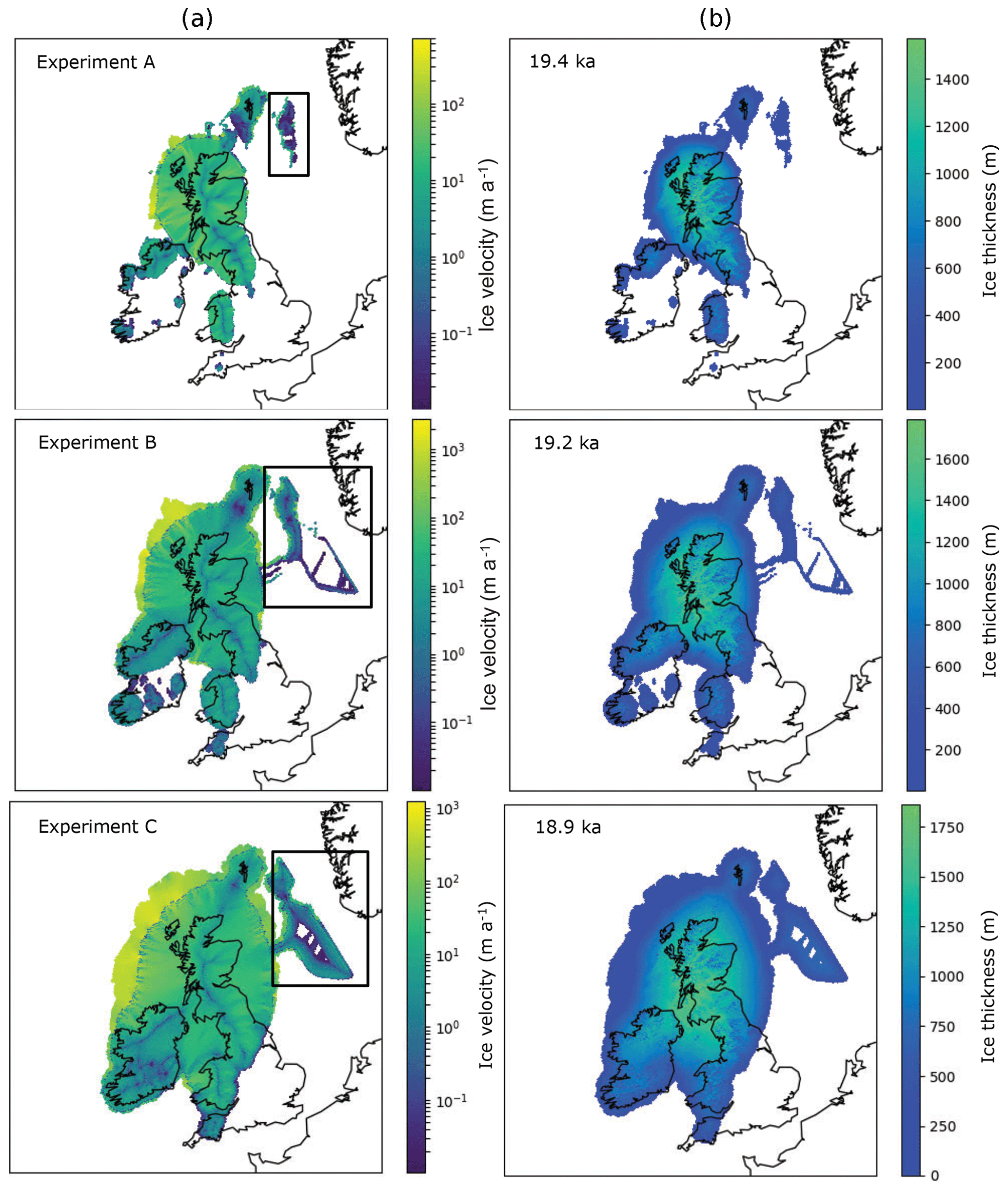
Figure 6Maximum extent of produced ice sheet for the three experiments. Experiment B is 1 ∘C colder than A, and Experiment C is 2 ∘C colder than A. Panel (a) shows ice velocity; panel (b) shows ice thickness. The boxes in the left panel (a) highlight likely erroneous output in the North Sea, likely a consequence of model domain, discussed further in the text.
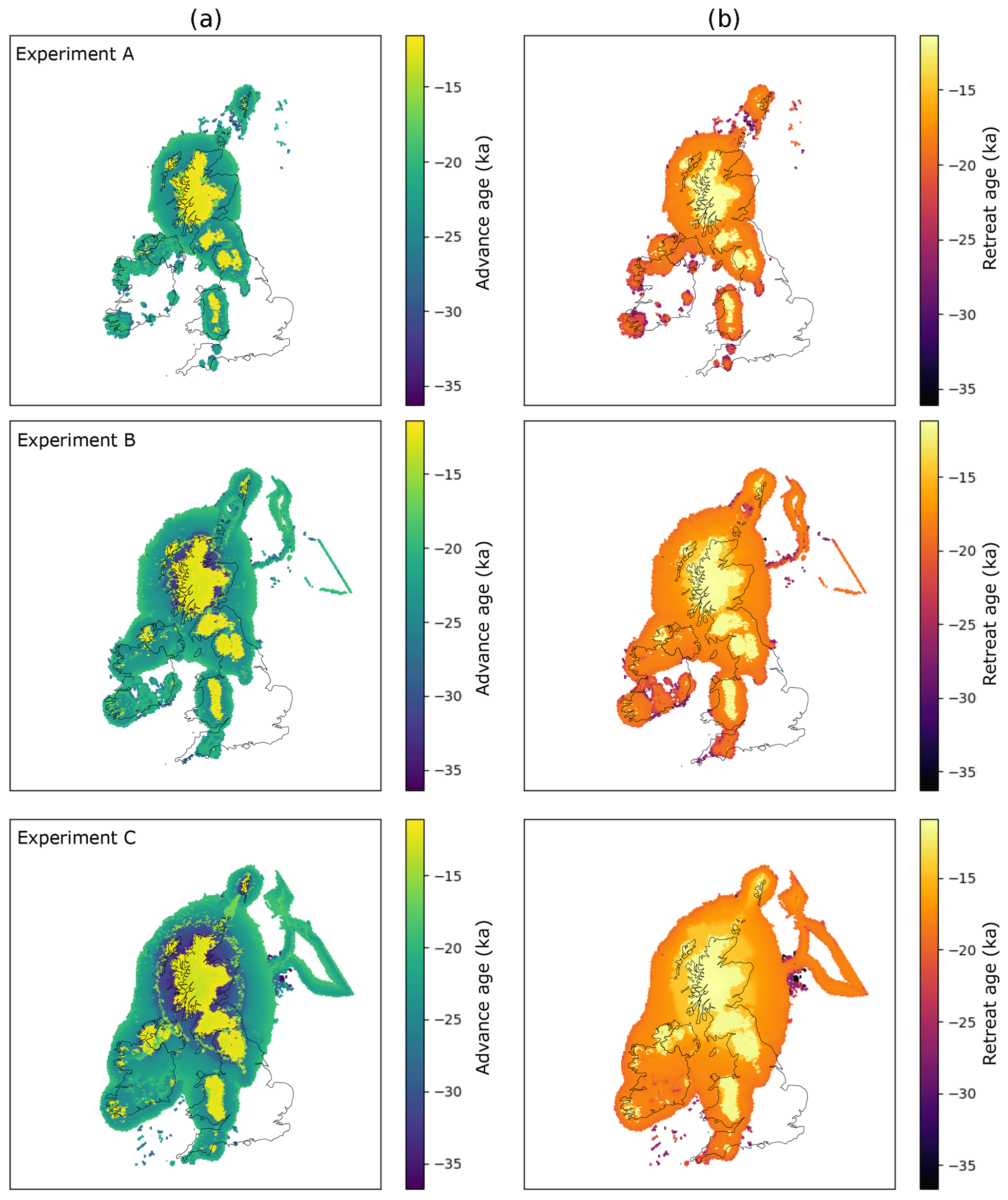
Figure 7Timing of advance (a) and retreat (b) from the three ice-sheet modelling experiments. Experiments are the same as in Fig. 6. The early ages toward the centre of the model, and centred over higher topography, represent the modelled extent of the Younger Dryas readvance.
4.2 Geochronological data
Ice-sheet advance dates were taken from the compilation of Hughes et al. (2016) and gridded to the ice-sheet model domain (Fig. 4). In total, 61 cells were represented with advance dates (Fig. 8a). Considering now ice-sheet retreat (Fig. 8b), dates deemed reliable or probably reliable by Small et al. (2017) were used (i.e. those given a “traffic light rating” of green or amber). For the dated advance and retreat locations, the geochronological data in each cell were assigned an error corresponding to that which was reported in the literature. We also compared our results to the “likely” empirical reconstruction of Hughes et al. (2016), based on that of Clark et al. (2012) (Fig. 8c), using the minimum and maximum bounding envelopes to assign an error to each cell of the ice-sheet grid (Fig. 8d). The largest errors occur in the North Sea region, where there is a lack of empirical data (e.g. Fig. 8a and b).
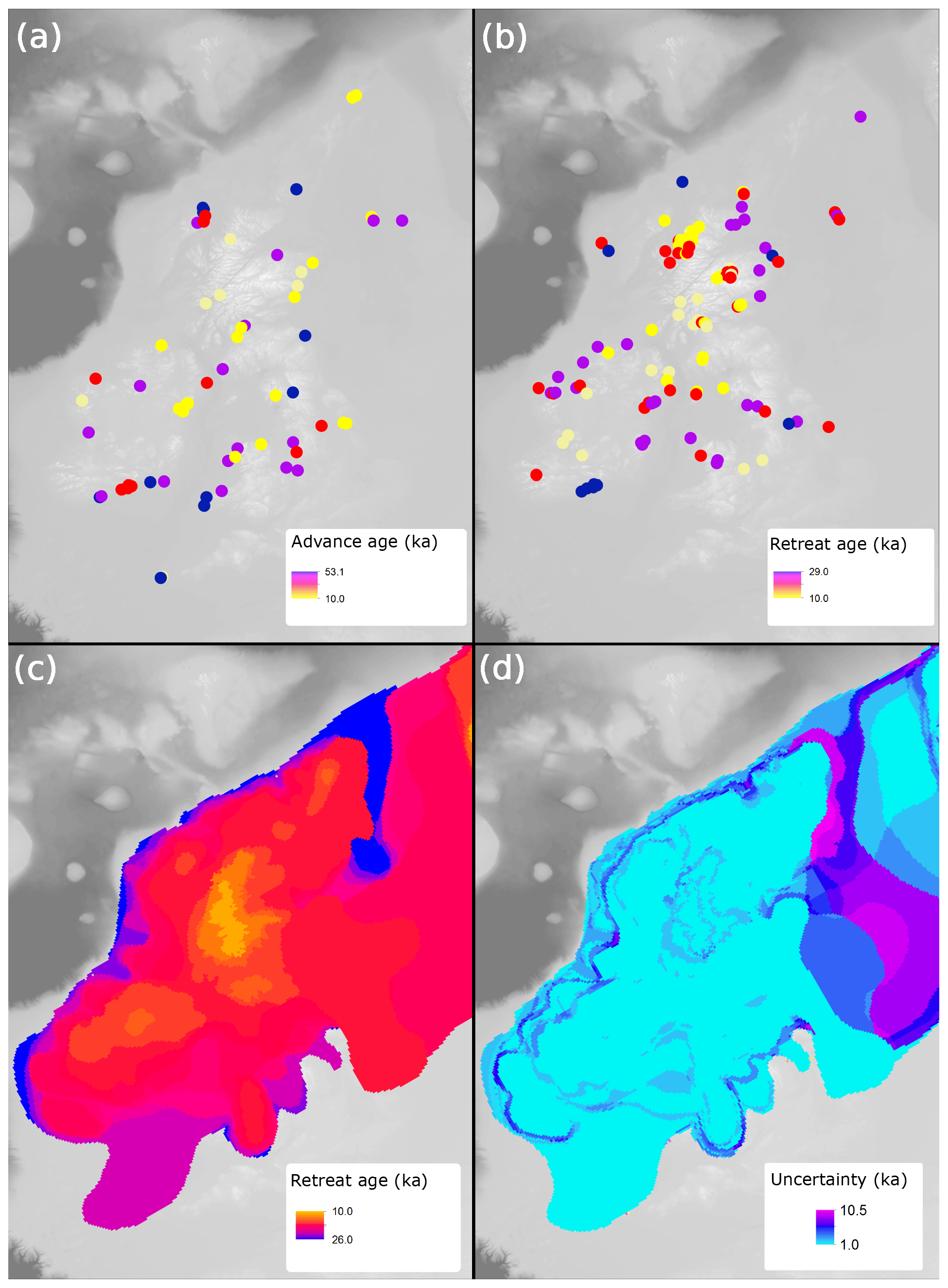
Figure 8Example of geochronological data projected onto model raster grids, as point data in panels (a) and (b), and from an empirical reconstruction in panels (c) and (d). (a) Advance ages from Hughes et al. (2016). (b) Retreat ages from Small et al. (2017). (c) Retreat age derived from DATED isochrone reconstruction (Hughes et al., 2016). (d) Error associated with reconstruction in panel (c).
4.3 Results
Table 4 shows selected statistics derived by ATAT when comparing the three ice-sheet modelling experiments (Figs. 6 and 7) against the three categories of data (advance, retreat, isochrones; Fig. 8). wRMSE was not calculated for the DATED isochrone reconstruction, as grid points are distributed evenly and therefore have equal spatial weighting (Table 4). Experiment C produces modelled ice sheets with the greatest areal extent and therefore performs best at correctly covering the dated areas (Table 4). However, none of the three experiments perform particularly well when compared with the data or the empirical reconstruction regarding timing and results in high (>2000-year) RMSEs (Table 4). The application of ATAT and the results from these simplified experiments allow us to suggest directions for analysing future experiments.
Table 4Example statistics from ATAT. Note that the RMSE is often altered by applying the spatial weighting to create wRMSE. “n/a” means “not applicable”.
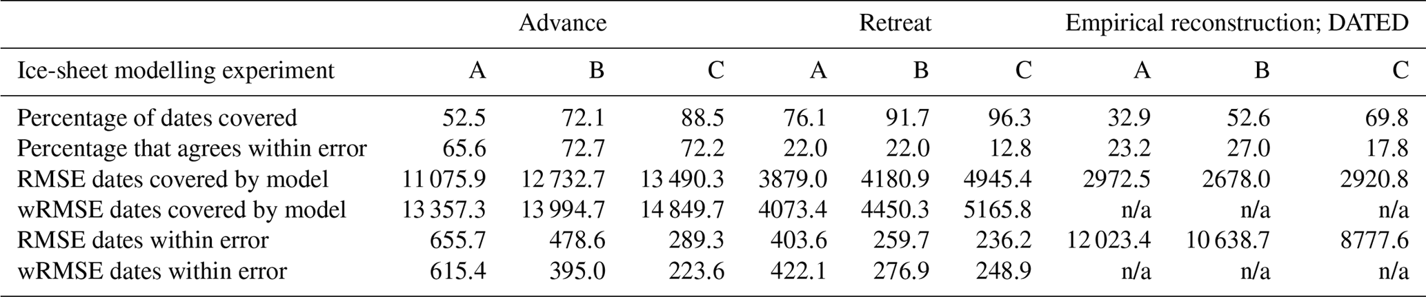
All three experiments produced large RMSEs, on the order of thousands of years, when compared to all three categories of data (Table 4). For advance ages, the three simulations conform to a large number of dated locations (e.g. 72 % of ages in Experiments B and C; Table 4). However, the RMSEs of advance ages are high (Table 4). This shows that, while the models perform well at matching the constraint of covering an area in ice after an advance age (Fig. 3), the models often glaciate a region much later than required. Advance dates are particularly difficult to obtain from the stratigraphic record, and often there may be a long hiatus between the initial deposition of dateable material and the subsequent advance of a glacier. Future experiments with large ensembles should therefore consider the number of advance dates conformed to (rather than the RMSE) as a more robust guide for model performance during ice advance.
For the retreat comparisons, the three modelling experiments conform to a larger percentage of sites, seemingly outperforming the empirically derived DATED reconstruction (Table 4). However, where model–data agreement occurs, the RMSEs produced are much higher when the model is compared to the DATED reconstruction. This is due to the reconstruction containing large uncertainties in regions which lack geochronological control (for example, in the North Sea; Fig. 8). These uncertainties, a product of spatial interpolation across regions with sparse information, are much greater than those associated with individual dates. Figure 9a shows examples of output maps from ATAT which display the spatial pattern of agreement and the magnitude of the difference between Experiment C and the DATED reconstruction. This shows that due to the uncertainty associated with North Sea glaciation, even where the model produces an unrealistic artefact, there is data–model agreement. Furthermore, ATAT produces a map which displays the number of years between data-based and modelled retreat and/or advance (e.g. Fig. 9b). Figure 9b, which compares Experiment C to the DATED isochrones, shows that the timing of model–data disagreement is spatially variable. If more modelling simulations were conducted, such maps may reveal regions of reconstruction or particular dates which are difficult to simulate in the model. In such cases, data or model re-evaluation may be required, and herein lies the potential utility of this ATAT tool in making sense of ensemble model runs. However, such model–data comparison awaits a full-ensemble simulation which accounts for model uncertainty (e.g. Hubbard et al., 2009).
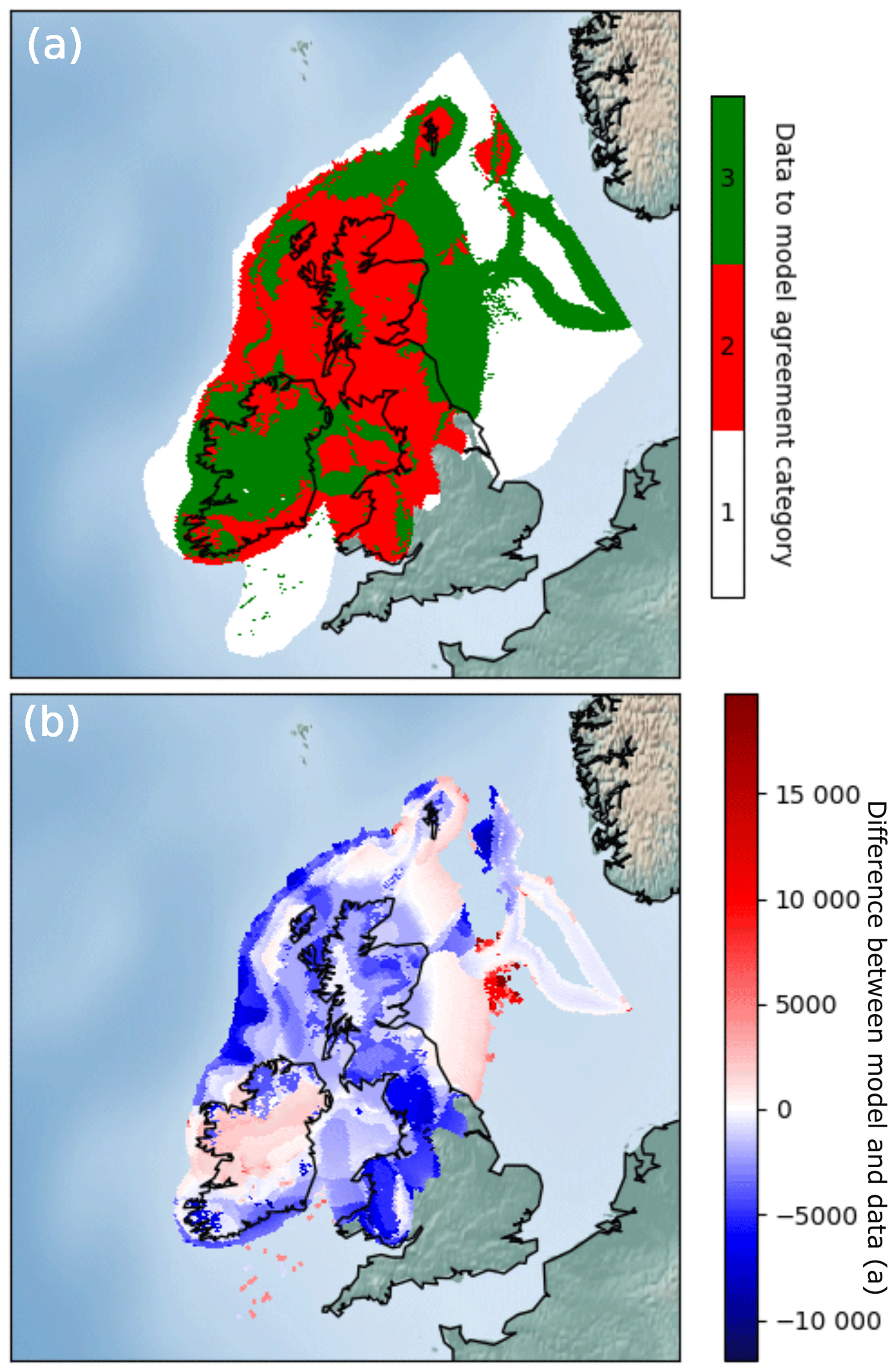
Figure 9Example mapped outputs from ATAT. In this case, Experiment C was compared with the DATED reconstruction. Panel (a) (cumulative agreement) shows categories of data–model agreement across the domain, where 1 indicates areas not covered by model, 2 indicates no agreement and 3 indicates data–model agreement within error. Panel (b) (model–data offset) shows magnitude of difference between model and data; negative values show a modelled retreat of ice later than the DATED isochrones, and positive values show a modelled retreat of ice before the DATED isochrones.
Here, we present ATAT, an automated timing accordance tool for comparing ice-sheet model output with geochronological data and empirical ice-sheet reconstructions. We demonstrate the utility of ATAT through three simplified simulations of the former British–Irish ice sheet. Note that a larger ensemble model of hundreds to thousands of runs is required for model evaluation (e.g. Hubbard et al., 2009). ATAT enables users to quantify the difference between the simulated timing of ice-sheet advance and retreat and those from a chosen dataset, and allows production of cumulative ice coverage agreement maps that should help distinguish between less and more promising runs. We envisage that this tool will be especially useful for ice-sheet modellers through justifying model choice from an ensemble, quantifying error and tuning ice-sheet model experiments to fit geochronological data. Ideally, this tool should be used in combination with other evaluation methods, such as fit to relative sea-level records. In the case where locations or regions of data cannot be fit by a model, and all model uncertainty has been accounted for in an ensemble simulation, the comparisons made in ATAT may also highlight that data re-evaluation is necessary. ATAT is supplied as the Supplement to this article.
ATAT 1.1 source code is freely distributed under a GNU GPL licence as the Supplement to this paper. It can also be downloaded with example input grids from https://doi.org/10.15131/shef.data.7172243 (Ely et al., 2019b). An example geochronological data grid and ice-sheet model grid can also be downloaded from this link. The ice-sheet modelling experiments shown here were conducted using the Parallel Ice Sheet Model (http://pism-docs.org/, last access: 8 October 2018). Development of PISM is supported by NASA grant NNX17AG65G and NSF grants PLR-1603799 and PLR-1644277. The geochronological data used are freely available from https://www.sciencedirect.com/science/article/pii/S0012825216304408\#s0105 (last access: 8 October 2018) and https://doi.org/10.1594/PANGAEA.848117 (Hughes et al., 2015).
General instructions: ATAT is written in Python and distributed as both .py script, for use in Python 2, and a .py3 script, for use with Python 3. The tool requires instillation of Python and the following freely available Python packages:
-
NetCDF4 (https://pypi.python.org/pypi/netCDF4, last access: 8 October 2018),
-
NumPy (http://www.numpy.org/, last access: 8 October 2018),
-
SciPy (https://www.scipy.org/, last access: 8 October 2018),
-
Matplotlib (https://matplotlib.org/, last access: 8 October 2018) and
-
Matplotlib toolkit basemap (https://matplotlib.org/basemap/, last access: 8 October 2018).
ATAT can be run from any Python-enabled environment (e.g. IDLE, BASH). Here, we provide the following simple instructions for running ATAT in a BASH shell. For numerous runs, a shell script should be created.
From the command line, launch the ATAT script using Python (“python ATATv1.1.py”). Eight command-line arguments (A1–A8), separated by a space should then follow.
-
A1 dictates whether deglacial or advance ages are being tested. Type “DEGLACIAL” or “ADVANCE” accordingly.
-
A2 is the path to the geochronological data file (e.g. “/home/ATAT/geochron.nc”).
-
A3 defines whether the model extent is based on thickness or a mask. Type THK or MSK accordingly.
-
A4 is the path to the ice-sheet model output file (e.g. “/home/ATAT/icesheetmodel1.nc”).
-
A5 is the value of the ice-sheet output mask. A value is required even if A3 = THK but can be any value as it will be ignored.
-
A6 to A8 control output maps. A6 defines whether the output map should consider margin uncertainty, with a value of BORDER or NONE.
-
A7 defines whether the model–data offset map displaces RMSE (option “NONE”) or wRMSE (“WEIGHTED”).
-
A8 specifies which dates are plotted on the difference map and can be “ALL” for all dates, “COVERED” for those which at some point where covered by ice and “INERROR” to display only those dates where model–data agreement within dating error occurred.
An example command would be “python ATATv1.1.py DEGLACIAL /home/ATAT/dated_recon.nc MSK /home/ATAT/experiment1.nc 2 BORDER WEIGHTED INERROR”. ATAT then outputs the two maps and a .csv table containing all derived statistics.
Input geochronological data can be created in a GIS environment such as ArcMap or QGIS. Here, the user must discern the appropriate geochronological data for each grid cell. Since geochronological data are usually stored as point data, these must be gridded to single grid points as positive values, with surrounding areas of no data assigned a value of 0. When comparing to a reconstruction (e.g. Hughes et al., 2016), cells outside the reconstruction should be assigned a value of 0. Those within the reconstruction should be assigned a value corresponding to the reconstructed age of retreat. The gridded data must be converted to NetCDF format, the details of which are shown in Table 3. We emphasise that the quality of geochronological data used must be considered, and an example of how to filter geochronological data is documented in Small et al. (2017). Ice thickness grids can be created using ice-sheet modelling software such as PISM (Winkelmann et al., 2011). The two grids (data and model) must be aligned and have the same size dimensions for use in ATAT. Examples are included as the Supplement, including a model output from Ely et al. (2019a).
The supplement related to this article is available online at: https://doi.org/10.5194/gmd-12-933-2019-supplement.
JCE led the preparation of the manuscript, designed the model experiments and wrote the ATAT code under the supervision of CDC and RCAH. DS provided advice on geochronology. All authors contributed to the writing of the manuscript.
The authors declare that they have no conflict of interest.
This work was supported by the Natural Environment Research Council
consortium grant; BRITICE-CHRONO NE/J009768/1. Development of PISM is
supported by NASA grant NNX17AG65G and NSF grants PLR-1603799 and
PLR-1644277. We thank Evan Gowan and Lev Tarasov for their constructive
reviews which improved the manuscript.
Edited by: Didier Roche
Reviewed by: Evan Gowan and Lev Tarasov
Applegate, P. J., Kirchner, N., Stone, E. J., Keller, K., and Greve, R.: An assessment of key model parametric uncertainties in projections of Greenland Ice Sheet behavior, The Cryosphere, 6, 589–606, https://doi.org/10.5194/tc-6-589-2012, 2012.
Arnold, J. R. and Libby, W. F.: Radiocarbon dates, Science, 113, 111–120, 1951.
Auriac, A., Whitehouse, P. L., Bentley, M. J., Patton, H., Lloyd, J. M., and Hubbard, A.: Glacial isostatic adjustment associated with the Barents Sea ice sheet: a modelling inter-comparison, Quaternary Sci. Rev., 147, 122–135, 2016.
Balco, G.: Contributions and unrealized potential contributions of cosmogenic-nuclide exposure dating to glacier chronology, 1990–2010, Quaternary Sci. Rev., 30, 3–27, 2011.
Bamber, J. L. and Aspinall, W. P.: An expert judgement assessment of future sea level rise from the ice sheets, Nat. Clim. Change, 3, 424–427, 2013.
Bateman, M. D., Evans, D. J., Roberts, D. H., Medialdea, A., Ely, J., and Clark, C. D.: The timing and consequences of the blockage of the Humber Gap by the last British-Irish Ice Sheet, Boreas, 47, 41–61, 2018.
Boulton, G. and Hagdorn, M.: Glaciology of the British Isles Ice Sheet during the last glacial cycle: form, flow, streams and lobes, Quaternary Sci. Rev., 25, 3359–3390, 2006.
Braconnot, P., Harrison, S. P., Kageyama, M., Bartlein, P. J., Masson-Delmotte, V., Abe-Ouchi, A., Otto-Bliesner, B., and Zhao, Y.: Evaluation of climate models using palaeoclimatic data, Nat. Clim. Change, 2, 417–424, 2012.
Briggs, R. D. and Tarasov, L.: How to evaluate model-derived deglaciation chronologies: a case study using Antarctica, Quaternary Sci. Rev., 63, 109–127, 2013.
Briggs, R. D., Pollard, D., and Tarasov, L.: A data-constrained large ensemble analysis of Antarctic evolution since the Eemian, Quaternary Sci. Rev., 103, 91–115, 2014.
Brown, E. J., Rose, J., Coope, R. G., and Lowe, J. J.: An MIS 3 age organic deposit from Balglass Burn, central Scotland: palaeoenvironmental significance and implications for the timing of the onset of the LGM ice sheet in the vicinity of the British Isles, J. Quaternary Sci., 22, 295–308, 2007.
Bueler, E. and Brown, J.: Shallow shelf approximation as a “sliding law” in a thermomechanically coupled ice sheet model, J. Geophys. Res.-Earth, 114, F03008, https://doi.org/10.1029/2008JF001179, 2009.
Bueler, E. D., Lingle, C. S., and Brown, J.: Fast computation of a viscoelastic deformable Earth model for ice-sheet simulations, Ann. Glaciol., 46, 97–105, 2007.
Calov, R. and Greve, R.: A semi-analytical solution for the positive degree-day model with stochastic temperature variations, J. Glaciol., 51, 173–175, 2005.
Chiverrell, R. C., Thrasher, I. M., Thomas, G. S., Lang, A., Scourse, J. D., van Landeghem, K. J., Mccarroll, D., Clark, C. D., Cofaigh, C.Ó., Evans, D. J., and Ballantyne, C. K.: Bayesian modelling the retreat of the Irish Sea Ice Stream, J. Quaternary Sci., 28, 200–209, 2013.
Clark, C. D., Hughes, A. L., Greenwood, S. L., Jordan, C., and Sejrup, H. P.: Pattern and timing of retreat of the last British-Irish Ice Sheet, Quaternary Sci. Rev., 44, 112–146, 2012.
Clark, C. D., Ely, J. C., Greenwood, S. L., Hughes, A. L. C., Meehan, R., Barr, I. D., Bateman, M. D., Bradwell, T., Doole, J., Evans, D. J. A., Joran, C. J., Monteys, X., Pellicier, X. M., and Sheehy, M.: BRITICE Glacial Map, version 2: a map and GIS database of glacial landforms of the last British-Irish Ice Sheet, Boreas, 47, 11–27, 2018.
Collins, M.: Ensembles and probabilities: a new era in the prediction of climate change, Philos. T. R. Soc. A, 365, 1957–1970, 2007.
Collins, M., Booth, B. B., Bhaskaran, B., Harris, G. R., Murphy, J. M., Sexton, D. M., and Webb, M. J.: Climate model errors, feedbacks and forcings: a comparison of perturbed physics and multi-model ensembles, Clim. Dynam., 36, 1737–1766, 2011.
Cornford, S. L., Martin, D. F., Graves, D. T., Ranken, D. F., Le Brocq, A. M., Gladstone, R. M., Payne, A. J., Ng, E. G., and Lipscomb, W. H.: Adaptive mesh, finite volume modeling of marine ice sheets, J. Comput. Phys., 232, 529–549, 2013.
DeConto, R. M. and Pollard, D.: Contribution of Antarctica to past and future sea-level rise, Nature, 531, 591–597, 2016.
Duller, G. A. T.: Single grain optical dating of glacigenic deposits, Quaternary Geochr., 1, 296–304, 2006.
Dyke, A. S.: An outline of North American deglaciation with emphasis on central and northern Canada, Dev. Quaternary Sci., 2, 373–424, 2004.
Edwards, T. L., Fettweis, X., Gagliardini, O., Gillet-Chaulet, F., Goelzer, H., Gregory, J. M., Hoffman, M., Huybrechts, P., Payne, A. J., Perego, M., Price, S., Quiquet, A., and Ritz, C.: Effect of uncertainty in surface mass balance-elevation feedback on projections of the future sea level contribution of the Greenland ice sheet, The Cryosphere, 8, 195–208, https://doi.org/10.5194/tc-8-195-2014, 2014.
Ely, J. C., Clark, C. D., Hindmarsh, R. C. A., Hughes, A. L. C., Greenwood, S. L., Bradley, S. L., Gasson, E., Gregoire, L., Gandy, N., Stokes, C. R., and Small, D.: An approach to combining geomorphological and geochronological data with ice sheet modelling, demonstrated using the last British-Irish Ice Sheet, J. Quaternary Sci., accepted, 2019a.
Ely, J. C., Clark, C. D., Small, D., and Hindmarsh, R. C. A.: ATAT code and example, data set, https://doi.org/10.15131/shef.data.7172243, 2019b.
Fowler, A. C.: A sliding law for glaciers of constant viscosity in the presence of subglacial cavitation, Proc. Roy. Soc. London A, 407, 147–170, 1986.
Fretwell, P., Pritchard, H. D., Vaughan, D. G., Bamber, J. L., Barrand, N. E., Bell, R., Bianchi, C., Bingham, R. G., Blankenship, D. D., Casassa, G., Catania, G., Callens, D., Conway, H., Cook, A. J., Corr, H. F. J., Damaske, D., Damm, V., Ferraccioli, F., Forsberg, R., Fujita, S., Gim, Y., Gogineni, P., Griggs, J. A., Hindmarsh, R. C. A., Holmlund, P., Holt, J. W., Jacobel, R. W., Jenkins, A., Jokat, W., Jordan, T., King, E. C., Kohler, J., Krabill, W., Riger-Kusk, M., Langley, K. A., Leitchenkov, G., Leuschen, C., Luyendyk, B. P., Matsuoka, K., Mouginot, J., Nitsche, F. O., Nogi, Y., Nost, O. A., Popov, S. V., Rignot, E., Rippin, D. M., Rivera, A., Roberts, J., Ross, N., Siegert, M. J., Smith, A. M., Steinhage, D., Studinger, M., Sun, B., Tinto, B. K., Welch, B. C., Wilson, D., Young, D. A., Xiangbin, C., and Zirizzotti, A.: Bedmap2: improved ice bed, surface and thickness datasets for Antarctica, The Cryosphere, 7, 375–393, https://doi.org/10.5194/tc-7-375-2013, 2013.
Fuchs, M. and Owen, L. A.: Luminescence dating of glacial and associated sediments: review, recommendations and future directions, Boreas, 37, 636–659, 2008.
Gasson, E., DeConto, R. M., Pollard, D., and Levy, R. H.: Dynamic Antarctic ice sheet during the early to mid-Miocene, P. Natl. Acad. Sci. USA, 113, 3459–3464, 2016.
Golledge, N. R., Levy, R. H., McKay, R. M., Fogwill, C. J., White, D. A., Graham, A. G., Smith, J. A., Hillenbrand, C. D., Licht, K. J., Denton, G. H., and Ackert, R. P.: Glaciology and geological signature of the Last Glacial Maximum Antarctic ice sheet, Quaternary Sci. Rev., 78, 225–247, 2013.
Gomez, N., Pollard, D., Mitrovica, J. X., Huybers, P., and Clark, P. U.: Evolution of a coupled marine ice sheet-sea level model, J. Geophys. Res., 117, F01013, https://doi.org/10.1029/2011JF002128, 2012.
Gomez, N., Pollard, D., and Mitrovica, J. X.: A 3-D coupled ice sheet–sea level model applied to Antarctica through the last 40 ky, Earth Planet Sci. Lett., 384, 88–99, 2013.
Gowan, E. J.: An assessment of the minimum timing of ice free conditions of the western Laurentide Ice Sheet, Quaternary Sci. Rev., 75, 100–113, 2013.
Gregoire, L. J., Payne, A. J., and Valdes, P. J.: Deglacial rapid sea level rises caused by ice-sheet saddle collapses, Nature, 487, 219–222, 2012.
Greve, R. and Hutter, K.: Polythermal three-dimensional modelling of the Greenland ice sheet with varied geothermal heat flux, Ann. Glaciol., 21, 8–12, 1995.
Greve, R., Wyrwoll, K. H., and Eisenhauer, A.: Deglaciation of the Northern Hemisphere at the onset of the Eemian and Holocene, Ann. Glaciol., 28, 1–8, 1999.
Gudmundsson, G. H.: Ice-shelf buttressing and the stability of marine ice sheets, The Cryosphere, 7, 647–655, https://doi.org/10.5194/tc-7-647-2013, 2013.
Gudmundsson, G. H., Krug, J., Durand, G., Favier, L., and Gagliardini, O.: The stability of grounding lines on retrograde slopes, The Cryosphere, 6, 1497–1505, https://doi.org/10.5194/tc-6-1497-2012, 2012.
Heroy, D. C. and Anderson, J. B.: Radiocarbon constraints on Antarctic Peninsula ice sheet retreat following the Last Glacial Maximum (LGM), Quaternary Sci. Rev., 26, 3286–3297, 2007.
Heyman, J., Stroeven, A. P., Harbor, J. M., and Caffee, M. W.: Too young or too old: evaluating cosmogenic exposure dating based on an analysis of compiled boulder exposure ages, Earth Planet Sci. Lett., 302, 71–80, 2011.
Hindmarsh, R. C.: Consistent generation of ice-streams via thermo-viscous instabilities modulated by membrane stresses, Geophys. Res. Lett., 36, L06502, https://doi.org/10.1029/2008GL036877, 2009.
Hubbard, A., Bradwell, T., Golledge, N., Hall, A., Patton, H., Sugden, D., Cooper, R., and Stoker, M.: Dynamic cycles, ice streams and their impact on the extent, chronology and deglaciation of the British–Irish ice sheet, Quaternary Sci. Rev., 28, 758–776, 2009.
Hughes, A. L., Greenwood, S. L., and Clark, C. D.: Dating constraints on the last British-Irish Ice Sheet: a map and database, J Maps, 7, 156–184, 2011.
Hughes, A. L., Clark, C. D., and Jordan, C. J.: Flow-pattern evolution of the last British Ice Sheet, Quaternary Sci. Rev., 89, 148–168, 2014.
Hughes, A. L., Gyllencreutz, R., Lohne, Ø. S., Mangerud, J., Svendsen, J. I.: DATED-1: compilation of dates and time-slice reconstruction of the build-up and retreat of the last Eurasian (British-Irish, Scandinavian, Svalbard-Barents-Kara Seas) Ice Sheets 40–10 ka. Department of Earth Science, University of Bergen and Bjerknes Centre for Climate Research, PANGAEA, https://doi.org/10.1594/PANGAEA.848117, 2015.
Hughes, A. L., Gyllencreutz, R., Lohne, Ø. S., Mangerud, J., and Svendsen, J. I.: The last Eurasian ice sheets–a chronological database and time-slice reconstruction, DATED-1, Boreas, 45, 1–45, 2016.
Hughes, T. J.: Is the West Antarctic ice sheet disintegrating?, J. Geophys. Res., 78, 7884–7910, 1973.
Huybrechts, P.: The Antarctic ice sheet during the last glacial-interglacial cycle: a three-dimensional experiment, Ann. Glaciol., 14, 115–119, 1990.
Imbrie, J., Hays, J. D., Martinson, D. G., McIntyre, A., Mix, A. C., Morley, J. J., Pisias, N. G., Prell, W. L., and Shackleton, N. J.: The orbital theory of Pleistocene climate: support from a revised chronology of the marine δ18O record, edited by: Berger, A., Imbrie, J., Hays, H., Kukla, G., and Saltzman, B., in: Milankovitch and Climate, Part I. D. Reidel Publishing, Dordrecht, 269–305, 1984.
Johnsen, S. J., Dahl-Jensen, D., Dansgaard, W., and Gundestrup, N.: Greenland palaeotemperatures derived from GRIP bore hole temperature and ice core isotope profiles, Tellus B, 47, 624–629, 1995.
Kirchner, N., Hutter, K., Jakobsson, M., and Gyllencreutz, R.: Capabilities and limitations of numerical ice sheet models: a discussion for Earth-scientists and modelers, Quaternary Sci. Rev., 30, 3691–3704, 2011.
Kirchner, N., Ahlkrona, J., Gowan, E. J., Lötstedt, P., Lea, J. M., Noormets, R., von Sydow, L., Dowdeswell, J. A., and Benham, T.: Shallow ice approximation, second order shallow ice approximation, and full Stokes models: A discussion of their roles in palaeo-ice sheet modelling and development, Quaternary Sci. Rev., 147, 136–147, 2016.
Kleman, J., Hättestrand, C., Stroeven, A. P., Jansson, K. N., De Angelis, H., and Borgström, I.: Reconstruction of Palaeo-Ice Sheets-Inversion of their Glacial Geomorphological Record, in: Glacier science and environmental change, edited by: Knight, P. G., 192–198, 2006.
Larour, E., Seroussi, H., Morlighem, M., and Rignot, E.: Continental scale, high order, high spatial resolution, ice sheet modeling using the Ice Sheet System Model (ISSM), J. Geophys. Res.-Earth, 117, F01022, https://doi.org/10.1029/2011JF002140, 2012.
Libby, W. F., Anderson, E. C., and Arnold, J. R.: Age determination by radiocarbon content: world-wide assay of natural radiocarbon, Science, 109, 227–228, 1949.
Lingle, C. S. and Clark, J. A.: A numerical model of interactions between a marine ice sheet and the solid earth: Application to a West Antarctic ice stream, J. Geophys. Res.-Oceans, 90, 1100–1114, 1985.
Livingstone, S. J., Cofaigh, C. Ó., Stokes, C. R., Hillenbrand, C. D., Vieli, A., and Jamieson, S. S.: Antarctic palaeo-ice streams, Earth-Sci. Rev., 111, 90–128, 2012.
Lorenz, E. N.: Deterministic Nonperiodic Flow, J. Atmos. Sci., 20, 130–141, 1963.
Lowe, J. J. and Walker, M. J.: Radiocarbon Dating the Last Glacial-Interglacial Transition (Ca. 14–9 14C Ka Bp) in Terrestrial and Marine Records: The Need for New Quality Assurance Protocols, Radiocarbon, 42, 53–68, 2000.
Lowell, T. V., Fisher, T. G., Hajdas, I., Glover, K., Loope, H., and Henry, T.: Radiocarbon deglaciation chronology of the Thunder Bay, Ontario area and implications for ice sheet retreat patterns, Quaternary Sci. Rev., 28, 1597–1607, 2009.
Lukas, S., Spencer, J. Q., Robinson, R. A., and Benn, D. I.: Problems associated with luminescence dating of Late Quaternary glacial sediments in the NW Scottish Highlands, Quaternary Geochron., 2, 243–248, 2007.
Mercer, J. H.: West Antarctic ice sheet and CO2 greenhouse effect: a threat of disaster, Nature, 271, 321–325, 1978.
Murphy, J. M., Sexton, D. M., Barnett, D. N., Jones, G. S., Webb, M. J., Collins, M., and Stainforth, D. A.: Quantification of modelling uncertainties in a large ensemble of climate change simulations, Nature, 430, 768–771, 2004.
Napieralski, J., Harbor, J., and Li, Y.: Glacial geomorphology and geographic information systems, Earth-Sci. Rev., 85, 1–22, 2007.
Ó Cofaigh, C. Ó. and Evans, D. J.: Radiocarbon constraints on the age of the maximum advance of the British–Irish Ice Sheet in the Celtic Sea, Quaternary Sci. Rev., 26, 1197–1203, 2007.
Patton, H., Hubbard, A., Andreassen, K., Winsborrow, M., and Stroeven, A. P.: The build-up, configuration, and dynamical sensitivity of the Eurasian ice-sheet complex to Late Weichselian climatic and oceanic forcing, Quaternary Sci. Rev., 153, 97–121, 2016.
Pattyn, F.: Sea-level response to melting of Antarctic ice shelves on multi-centennial timescales with the fast Elementary Thermomechanical Ice Sheet model (f.ETISh v1.0), The Cryosphere, 11, 1851–1878, https://doi.org/10.5194/tc-11-1851-2017, 2017.
Pattyn, F., Perichon, L., Aschwanden, A., Breuer, B., de Smedt, B., Gagliardini, O., Gudmundsson, G. H., Hindmarsh, R. C. A., Hubbard, A., Johnson, J. V., Kleiner, T., Konovalov, Y., Martin, C., Payne, A. J., Pollard, D., Price, S., Rückamp, M., Saito, F., Soucek, O., Sugiyama, S., and Zwinger, T.: Benchmark experiments for higher-order and full-Stokes ice sheet models (ISMIP-HOM), The Cryosphere, 2, 95–108, https://doi.org/10.5194/tc-2-95-2008, 2008.
Pollard, D. and DeConto, R. M.: Modelling West Antarctic ice sheet growth and collapse through the past five million years, Nature, 458, 329–332, 2009.
Ritz, C., Edwards, T. L., Durand, G., Payne, A. J., Peyaud, V., and Hindmarsh, R. C.: Potential sea-level rise from Antarctic ice-sheet instability constrained by observations, Nature, 528, 115–118, 2015.
Robinson, A., Calov, R., and Ganopolski, A.: Greenland ice sheet model parameters constrained using simulations of the Eemian Interglacial, Clim. Past, 7, 381–396, https://doi.org/10.5194/cp-7-381-2011, 2011.
Rougier, J.: Probabilistic inference for future climate using an ensemble of climate model evaluations, Clim. Change, 81, 247–264, 2007.
Rutt, I. C., Hagdorn, M., Hulton, N. R. J., and Payne, A. J.: The Glimmer community ice sheet model, J. Geophys. Res.-Earth, 114, F02004, https://doi.org/10.1029/2008JF001015, 2009.
Schoof, C. S.: Ice sheet grounding line dynamics: steady states, stability and hysteresis, J. Geophys. Res.-Earth Surf., 112, F03S28, https://doi.org/10.1029/2006JF000664, 2007.
Schoof, C.: Coulomb friction and other sliding laws in a higher-order glacier flow model, Math. Mod. Meth. Appl. S, 20, 157–189, 2010.
Schoof, C.: Marine ice sheet stability, J. Fluid Mech., 698, 62–72, 2012.
Seddik, H., Greve, R., Zwinger, T., Gillet-Chaulet, F., and Gagliardini, O.: Simulations of the Greenland ice sheet 100 years into the future with the full Stokes model Elmer/Ice, J. Glaciol., 58, 427–440, 2012.
Seguinot, J., Rogozhina, I., Stroeven, A. P., Margold, M., and Kleman, J.: Numerical simulations of the Cordilleran ice sheet through the last glacial cycle, The Cryosphere, 10, 639–664, https://doi.org/10.5194/tc-10-639-2016, 2016.
Simpson, M. J., Milne, G. A., Huybrechts, P., and Long, A. J.: Calibrating a glaciological model of the Greenland ice sheet from the Last Glacial Maximum to present-day using field observations of relative sea level and ice extent, Quaternary Sci. Rev., 28, 1631–1657, 2009.
Small, D., Clark, C. D., Chiverrell, R. C., Smedley, R. K., Bateman, M. D., Duller, G. A., Ely, J. C., Fabel, D., Medialdea, A., and Moreton, S. G.: Devising quality assurance procedures for assessment of legacy geochronological data relating to deglaciation of the last British-Irish Ice Sheet, Earth-Sci. Rev., 164, 232–250, 2017.
Smedley, R. K., Glasser, N. F., and Duller, G. A. T.: Luminescence dating of glacial advances at Lago Buenos Aires (∼46∘S), Patagonia, Quaternary Sci. Rev., 134, 59–73, 2016.
Smedley, R. K., Chiverrell, R. C., Ballantyne, C. K., Burke, M. J., Clark, C. D., Duller, G. A. T., Fabel, D., McCarroll, D., Scourse, J. D., Small, D., and Thomas, G. S. P.: Internal dynamics condition centennial-scale oscillations in marine-based ice-stream retreat, Geology, 45, 787–790, 2017.
Stokes, C. R., Tarasov, L., Blomdin, R., Cronin, T. M., Fisher, T. G., Gyllencreutz, R., Hättestrand, C., Heyman, J., Hindmarsh, R. C., Hughes, A. L., and Jakobsson, M.: On the reconstruction of palaeo-ice sheets: recent advances and future challenges, Quaternary Sci. Rev., 125, 15–49, 2015.
Tarasov, L. and Peltier, W. R.: A geophysically constrained large ensemble analysis of the deglacial history of the North American ice-sheet complex, Quaternary Sci. Rev., 23, 359–388, 2004.
Tarasov, L., Dyke, A. S., Neal, R. M., and Peltier, W. R.: A data-calibrated distribution of deglacial chronologies for the North American ice complex from glaciological modeling, Earth Planet Sci. Lett., 315, 30–40, 2012.
Tebaldi, C. and Knutti, R.: The use of the multi-model ensemble in probabilistic climate projections, Philos. T. R. Soc. A, 365, 2053–2075, 2007.
Tushingham, A. M. and Peltier, W. R.: Validation of the ICE-3G Model of Würm-Wisconsin Deglaciation using a global data base of relative sea level histories, J. Geophys. Res.-Solid Earth, 97, 3285–3304, 1992.
Weertman, J.: Stability of the junction of an ice-sheet and an ice-shelf, J. Glaciol., 13, 3–11, 1974.
Winkelmann, R., Martin, M. A., Haseloff, M., Albrecht, T., Bueler, E., Khroulev, C., and Levermann, A.: The Potsdam Parallel Ice Sheet Model (PISM-PIK) – Part 1: Model description, The Cryosphere, 5, 715–726, https://doi.org/10.5194/tc-5-715-2011, 2011.