the Creative Commons Attribution 4.0 License.
the Creative Commons Attribution 4.0 License.
 | 13 Dec 2019
Sensitivity studies with the regional climate model COSMO-CLM 5.0 over the CORDEX Central Asia Domain
Emmanuele Russo
Ingo Kirchner
Stephan Pfahl
Martijn Schaap
Ulrich Cubasch
Due to its extension, geography and the presence of several underdeveloped or developing economies, the Central Asia domain of the Coordinated Regional Climate Downscaling Experiment (CORDEX) is one of the most vulnerable regions on Earth to the effects of climate changes. Reliable information on potential future changes with high spatial resolution acquire significant importance for the development of effective adaptation and mitigation strategies for the region. In this context, regional climate models (RCMs) play a fundamental role.
In this paper, the results of a set of sensitivity experiments with the regional climate model COSMO-CLM version 5.0, for the Central Asia CORDEX domain, are presented. Starting from a reference model setup, general model performance is evaluated for the present day, testing the effects of singular changes in the model physical configuration and their mutual interaction with the simulation of monthly and seasonal values of three variables that are important for impact studies: near-surface temperature, precipitation and diurnal temperature range. The final goal of this study is two-fold: having a general overview of model performance and its uncertainties for the considered region and determining at the same time an optimal model configuration.
Results show that the model presents remarkable deficiencies over different areas of the domain. The combined change of the albedo, taking into consideration the ratio of forest fractions, and the soil conductivity, taking into account the ratio of liquid water and ice in the soil, allows one to achieve the best improvements in model performance in terms of climatological means. Importantly, the model seems to be particularly sensitive to those parameterizations that deal with soil and surface features, and that could positively affect the repartition of incoming radiation. The analyses also show that improvements in model performance are not achievable for all domain subregions and variables, and they are the result of a compensation effect in the different cases. The proposed better performing configuration in terms of mean climate leads to similar positive improvements when considering different observational data sets and boundary data employed to force the simulations. On the other hand, due to the large uncertainties in the variability estimates from observations, the use of different boundaries and the model internal variability, it has not been possible to rank the different simulations according to their representation of the monthly variability.
This work is the first ever sensitivity study of an RCM for the CORDEX Central Asia domain and its results are of fundamental importance for further model development and for future climate projections over the area.
- Article
(9866 KB) - Full-text XML
-
Supplement
(2385 KB) - BibTeX
- EndNote


Regional climate models (RCMs) are a fundamental tool for the study of climate change, allowing one to reproduce the climate system with a high quality of details and to provide information at a regional scale. Their use for future climate projections constitutes indeed a vital resource for policy makers in decision making facing the threat of future global warming (Kim et al., 2014).
The Coordinated Regional Climate Downscaling Experiment (CORDEX; Giorgi et al., 2009) is an initiative sponsored by the World Climate Research Programme, aiming to coordinate international regional climate downscaling experiments. CORDEX sets a number of directives, including predefined resolution, regions, output variables and formats, to facilitate analysis of possible future climate changes (Nikulin et al., 2012).
Among the different CORDEX regions, Central Asia represents one of the largest domains, covering parts of Europe, Africa and almost the entire Asian continent. The domain extends from eastern Europe to the eastern part of China and from the northern part of India and the Arabian Peninsula in the south, to Siberia and the Arctic Ocean (Barents and Kara seas) in the north. It includes, almost entirely, two of the most important and populous countries: China and Russia. The region, despite being mainly characterized by arid and semi-arid climatic conditions, presents a wide variety of climatic zones, from the desert zones of the Gobi and the Arabian Peninsula, to the cold and dry areas of Siberia and the wet Northern Indian Monsoon region (Ozturk et al., 2017). Therefore, it offers the unique opportunity to test the model sensitivity to different climatic conditions at once.
Beside its importance from a modeling perspective, the extension, geography and the presence of several underdeveloped or developing economies makes the CORDEX Central Asia domain one of the most vulnerable regions on Earth to the effects of climate changes. Even small changes in climate conditions could dramatically affect ecosystems, agricultural crops, water resources, human health and livelihood of the region (Siegfried et al., 2012; Lioubimtseva et al., 2005; Lioubimtseva and Henebry, 2009; Liu et al., 2013; Yong-Jian et al., 2013; Zhen-Feng et al., 2013; Wang et al., 2017; Chuluunkhuyag, 2008; Diniega, 2012; Macias-Fauria et al., 2012). In this context, reliable information on potential future changes with high spatial resolution acquire significant importance for the development of effective adaptation and mitigation strategies.
The recognized prerequisite that every climate model has to satisfy in order to provide reliable future climate projections is the ability of realistically simulating present-day climate (Kim et al., 2014; Nature-Editorial-Board, 2010; Kim and Lee, 2003). Assessing the ability of a climate model to simulate the current climate is defined as model evaluation (Airey and Hulme, 1995). Model evaluation consists of an assessment of model quality and deficiencies originating from different modeling assumptions, conducted through the comparison of model outputs and observations (Kim et al., 2014; Kim and Lee, 2003; Flato et al., 2013; Lenderink, 2010; Overpeck et al., 2011; Bellprat et al., 2012a, b). Evaluation experiments normally consist of a set of present-day simulations conducted in a perfect boundary setting, i.e., using reanalysis products as lateral boundary forcings. This “modus operandi” allows for the separation of possible model biases from biases due to erroneous large-scale forcings, thus highlighting specific model deficiencies (Kotlarski et al., 2014). These may be related to the model formulation and to choices in model configuration (Awan et al., 2011; Bellprat et al., 2012a, b; de Elía et al., 2008; Evans et al., 2012). In the second case, it should be possible to improve model performance by testing different model configuration setups and choosing the one that better agrees with observations. This approach might be conceived as an optimization step. Nevertheless, it is important to emphasize the fact that a specific model configuration could produce better results by simply compensating for some deficiencies in the model formulation (Hourdin et al., 2017).
In climate models, the complexity and small spatial scales of the physical processes involved requires the so-called parameterization of many of these processes: this basically consists of summarizing physical phenomena and their interaction across different spatial and temporal scales (Fernández et al., 2007; Rummukainen, 2010; McFarlane, 2011; Hourdin et al., 2017), which is associated with substantial uncertainties. The same processes may be described through different parameterizations, with a different degree of complexity and infinitive parameter values. Consequently, the outcomes of a climate model might largely differ, depending on the parameterizations used and the selected parameters inputs. Additionally, the use of different forcings data sets, for example for greenhouse gases, aerosols or land cover changes, might have a significant effect on the results. Further, other details that need to be considered when configuring a climate model simulation for a defined domain are the configuration and spatial resolution of the model grid (both horizontally and vertically) and the coupling with different models representative of other components of the climate system. For regional climate models, all these aspects are domain dependent (Jacob et al., 2007, 2012; Rockel et al., 2008). This means that a regional climate modeler should always evaluate different model configurations, isolating the one that leads to a better agreement with observations, for each investigated region and employed model. In doing so, several sources of uncertainties should be taken into consideration: the fact that performance of the RCM for a specific region might vary according to the boundary conditions, the model internal variability and observational data sets should be acknowledged when evaluating model performance.
RCMs evaluation and configuration have been the subject of a large number of studies, for different regions, such as in Kotlarski et al. (2014), Umakanth and Kesarkar (2018), Borge et al. (2008), García-Díez et al. (2013), Crétat et al. (2012), Rajeevan et al. (2010), Diro et al. (2012), Giorgi et al. (2012), Reboita et al. (2014), Li et al. (2018) and Huang et al. (2015). For the RCM considered in this study, the COSMO-CLM (Rockel et al., 2008), Europe has received greater attention. Bellprat et al. (2012b) applied a quadratic metamodel on a subsample of model parameters in order to objectively tune the model for the region. Their method is considered the reference for COSMO-CLM for determining optimal parameters values and has been further developed and applied to the Mediterranean region by Avgoustoglou et al. (2017) and for higher resolution for the Alpine region by Voudouri et al. (2018). Bellprat et al. (2016) additionally used the same method for the European and the North American domain, finding quite similar values of optimal model parameters for the two regions. Using a more subjective approach, Montesarchio et al. (2012) conducted a set of sensitivity studies in order to determine the best model setup for the simulation of near-surface temperature and precipitation over northern and central Italy, at a spatial resolution of ∼8 km. Despite several important findings, they were not able to determine an optimal model configuration with respect to these variables. The alpine region was the subject of a study with COSMO-CLM by Suklitsch et al. (2008), where they found that changes in model resolution has a greater impact on model simulation than modifying dynamical and numerical schemes. Bachner et al. (2008) conducted a similar work for Germany, focusing on model performance for summer precipitation, concluding that the model uncertainty due to the modified physical parameterizations is considerable and highlighting the need for conducting evaluation and sensitivity studies prior to the application of a model for climate change projections. Studies investigating COSMO-CLM sensitivity for regions outside of Europe are more rare. Lange et al. (2015) tested model performance regarding different convection and non-precipitating subgrid-scale clouds parameterizations for South America. Through this work they managed to reduce long-standing model biases in precipitation for the region, by using the Integrated Forecasting System (IFS, Bechtold et al., 2008) of the European Centre for Medium-range Weather Forecasts (ECMWF) convection scheme and statistical schemes for subgrid-scale clouds. Bucchignani et al. (2016) compared the performance of 26 different model configurations for the Middle East–North Africa (MENA) CORDEX domain. They found that the model is particularly sensitive to changes in physical and tuning parameters for the region. In particular, they obtained best model performance with the representation of the albedo based on Moderate Resolution Imaging Spectroradiometer (MODIS, Lawrence and Chase, 2007) data, and a parameterization of aerosol based on the NASA-GISS Aerosol Optical Depth distributions (Tegen et al., 1997). Finally, Bucchignani et al. (2012) evaluated several configurations for northwestern China at a spatial resolution of approximately ∼8 km, even though they did not propose an optimal configuration for the region.
So far, neither an evaluation nor a sensitivity study on the impact of different configurations of an RCM have been documented for the CORDEX Central Asia domain. Such analyses are required to guide further model development and applications for the region: if we want to produce future climate projections for the region, we need to investigate model performance and deficiencies for the area and propose optimal model configurations.
In the light of the upcoming phase of the CORDEX initiative, denominated CORDEX – Coordinated Output for Regional Evaluations (CORE; Gutowski Jr. et al., 2016), in this paper the results of a set of sensitivity experiments with the regional climate model COSMO-CLM version 5.0, for the Central Asia CORDEX domain, are presented. From this perspective, this work represents the first step for the production of climate projections for the Central Asia domain using COSMO-CLM, evaluating general model performance, isolating the effects of different uncertainty sources on model results and determining an optimal model configuration for a region for which almost no reference exists. Starting from a reference model setup, general model performance is evaluated, testing the effects of a set of singular physical options and their mutual interaction, as well as two different forcing data sets on the simulation of monthly and seasonal values of three variables that are important for impact studies. These are near-surface temperature (T2M), precipitation (PRE) and diurnal temperature range (DTR), the third representing the daily excursion between maximum and minimum temperature, which is particularly important in terms of human body adaptability and stress. The final goal of this study is two-fold: having a general overview of model performance and its uncertainties for the considered region and determining at the same time a “best” suitable model configuration.
In Sect. 2 of this paper, the model, the different data sets and the methods employed in this study are described. Then, in Sect. 3, the results are presented. Finally, conclusions are outlined, with a general discussion of model performance and the proposal of a final optimal model configuration for the area of study.
In this section the research methods are described, including details on the model and the different simulation setups, the observational data sets used for the evaluation of model results and the employed metrics.
2.1 Model and experiment description
The Consortium for Small-Scale Modeling in Climate Mode (COSMO-CLM) is a non-hydrostatic regional climate model developed by the CLM community, an open international network of scientists. The model version employed in this study is the COSMO-CLM 5.0_clm9. Many studies have been conducted in recent years over different CORDEX regions, using COSMO-CLM (Panitz et al., 2014; Dobler and Ahrens, 2010; Bucchignani et al., 2016; Smiatek et al., 2016; Jacob et al., 2014; Kotlarski et al., 2014; Zhou et al., 2016).
The simulations presented in this study are performed with a spatial resolution of 0.22∘, as specified in the new CORDEX-CORE directives (Gutowski Jr. et al., 2016), on a rotated geographical grid. The initial simulation domain extends from ∼3 to ∼145∘ longitude and from ∼16 to ∼73∘ latitude. The domain includes a model relaxation zone of ∼250 km on each domain side, used to “relax” the model variables towards the driving data (Køltzow, 2012; Davies, 1976). Results of the simulation for this area are excluded from the analysis, with the final domain extent shown in Fig. 1. If not otherwise specified, all the simulations are run over a 15-year period from 1991 to 2005, with the first 5 years excluded from the analysis and considered as spinup time.
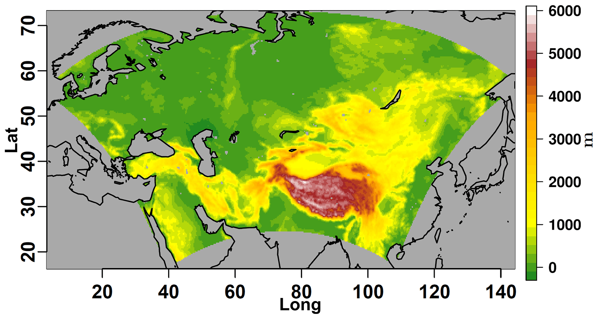
Figure 1Orography map of the Central Asia simulation domain at a spatial resolution of 0.22∘. Terrain height information is derived from the Global Land One-kilometer Base Elevation (GLOBE; GLOBE Task Team and others, 1999) data set.
In a set of sensitivity experiments labeled from a to q in the first section of Table 1, the effects on model performance of different changes in the model configuration are tested, first individually and then combining them with each other. The setup of experiment a is the reference from which the other experiments are configured, by implementing the modifications specified in the table. The model configuration used for the reference simulation is the same used for the CORDEX East Asia domain for the COSMO-CLM model version 5.0. This was considered as a good reference for the purposes of this study since the two regions share a large part of their domains. A general description of the setup of the reference simulation is provided in Table 2.
(Kinne et al., 2005)Table 1List of performed experiments and their corresponding configuration.
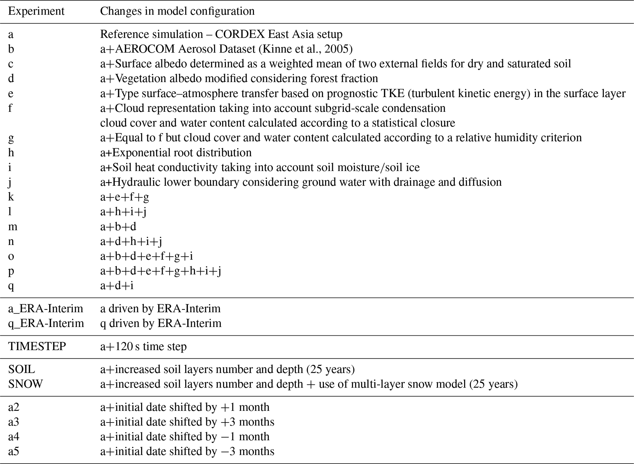
Table 2General description of model setup of the reference simulation a.

All the performed simulations are driven by the NCEP version 2 reanalysis data (Kanamitsu et al., 2002), provided as boundary and initial conditions. The boundaries have a temporal resolution of 6 h and a spectral resolution of T62 (∼1.89∘). NCEP2 data have been selected as boundary data, instead of commonly employed ERA-Interim reanalyses (Dee et al., 2011), since their resolution is closer to the resolution of the three global circulation models (GCMs) that are used for CORDEX-CORE simulations in the CLM community: MPI-ESM (Giorgetta et al., 2013), HadGEM (The HadGEM2 Development Team, 2011) and NorESM (Bentsen et al., 2013; Iversen et al., 2013), with a spatial resolution of, respectively, , and km. Thus, using NCEP2 as drivers allows one to reproduce a resolution jump more similar to the one present when using the considered GCMs.
Acknowledging the fact that ERA-Interim reanalysis data, which have a spectral resolution of T255 (∼0.7∘), are normally employed for the evaluation of RCMs, two additional simulations are performed, driven by ERA-Interim (second section of Table 1). This allows one to estimate the effects of the two different driving data on the simulations results and to support possible conclusions on an optimal setup, verifying how significantly the results differ in the two cases.
In order to better discriminate different sources of uncertainties in the model simulations, a run covering the period 1991–2005 is also performed (third section of Table 1), using a time step of 120 s, instead of that of the reference simulation of 150 s.
Two 25-year simulations, covering the period 1991–2015, are performed for testing different configurations that could help in reducing model biases over areas characterized by the presence of permafrost in winter. The two simulations, labeled SOIL and SNOW in the fourth section of Table 1, are performed increasing in both the number of soil layers from 10 to 13, together with their total depth from approximately 15 m to more than 130 m, and, only for SNOW, additionally using the multi-layer snow model of COSMO-CLM (Machulskaya, 2015). These simulations cover a longer period than the others since a longer spinup time is necessary in order to account for more and deeper soil layers. Their results, excluded from the direct comparison with the other simulations, are discussed in the results and concluding sections of this paper.
Finally, a set of four simulations are additionally performed for the investigation of the model internal variability (last section of Table 1). These simulations have the same setup as the reference simulation a, but are initialized at four different dates, shifted by ±1 and ±3 months with respect to the reference one.
All the proposed simulations are designed with the goal of better understanding main model limitations for the area and to which degree they can be reduced by properly configuring the model, isolating the effects of different sources of uncertainties.
2.2 Observations
Gridded observational data sets are used to compare model results against observational data on a similar scale. These gridded data sets are obtained through statistical extrapolations of surface observations. In addition to uncertainties related to the original measurements, these data sets also contain important uncertainties due to the statistical extrapolation procedure (Flaounas et al., 2012; Gómez-Navarro et al., 2012). For climate model evaluation studies, these uncertainties are usually taken into account by using a range of different data sets (Collins et al., 2013; Gómez-Navarro et al., 2012; Bellprat et al., 2012a, b; Flaounas et al., 2012; Lange et al., 2015; Zhou et al., 2016; Solman et al., 2013).
In this study, the issue of observational uncertainties is addressed by considering three different data sets for each of the investigated variables. The data sets include both observations and reanalysis data. For all three considered variables, information is retrieved from the CRU TS4.1 observational data set (Harris and Jones, 2017). Information on T2M and PRE is also retrieved from the University of Delaware (UDEL) gridded data set (Willmott, 2000), provided by the NOAA/OAR/ESRL PSD (Physical Science Division), Boulder, Colorado, USA. For T2M and DTR, in addition, the Modern-Era Retrospective analysis for Research and Applications, version 2 (MERRA2; Gelaro et al., 2017) is employed. For precipitation, the third considered data set is the Global Precipitation Climatology Centre data set (GPCC; Becker et al., 2011), while the ERA-Interim reanalysis data set (Dee et al., 2011) is used in addition to MERRA2 and to CRU for the evaluation of DTR.
All the data sets are retrieved on a grid with the same spatial resolution of 0.5∘. The ERA-Interim data, that originally have a horizontal resolution of approximately 80 km, are interpolated to the same grid resolution. The output of the simulations is upscaled to the same 0.5∘ grid of the observations. For temperature and diurnal temperature range, a bilinear remapping method is used for the upscaling, while for precipitation a conservative remapping method is employed.
Figure 2 shows the spread of the different observational data sets for each variable, for yearly, winter and summer climatological means over the period 1996–2005. As evident, large differences emerge among the different data sets, in particular for regions characterized by complex topography and lower observational stations density, such as the Tibetan Plateau and Siberia. The given spread could make it hard to quantify model biases over certain regions. In the case of T2M and DTR, the spread is certainly influenced by the fact that some of the data sets are reanalyses. Nevertheless, for T2M, differences exceeding 8∘ are present, in particular in winter, even between the CRU and the UDEL, over regions where the interpolation is highly affected by the low number of stations (Matsuura and Wilmott, 2012; Bucchignani et al., 2014). For PRE, the spread in the different observations (expressed in percentage with respect to the GPCC values) is remarkable in winter over the Tibetan Plateau and in summer over particularly dry areas. Despite the face that the differences might likely be influenced by the employed interpolation methods in each case, the spatial coverage of observation is still considered their main driver (Dong and Sun, 2018; Matsuura and Wilmott, 2012; Sun et al., 2018; Naumann et al., 2014).
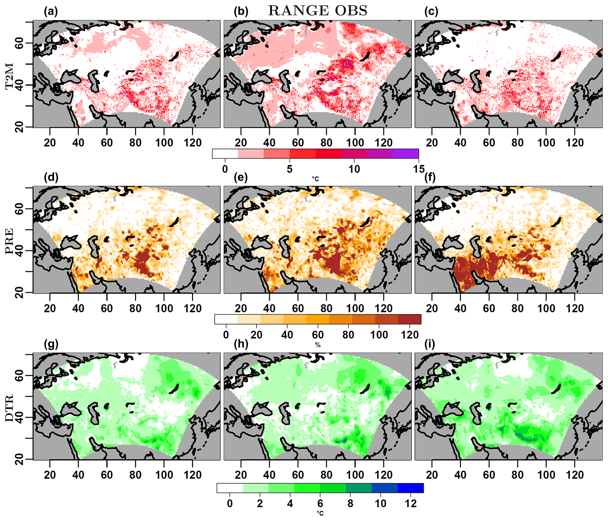
Figure 2Maps of the spread calculated among different observational data sets, for each considered variable, for the annual (a, d, g), winter (b, e, h) and summer means (c, f, i). From top to bottom, the values for near-surface temperature (T2M, ∘C), relative precipitation (PRE, %) and diurnal temperature range (DTR, ∘C, bottom panel) are respectively represented.
2.3 Analysis details and evaluation metrics
In order to rank different model configurations according to their skills in simulating the three considered variables over the region, their performance is evaluated with respect to those of the reference simulation (a, Table 2).
Since in the context of CORDEX simulations the main interest is often in the comparison of the mean climate between two different periods in time, the primary focus of the proposed analyses is on climatological monthly values of the considered variables: monthly values of daily means of T2M and DTR are considered, while for PRE integrated values are used. In addition, the results are supported by the investigation of the simulated monthly variability.
In the latter case, since the model is not expected to exactly match the observed temporal evolution of the investigated variables point by point (Gleckler et al., 2008; Wilks, 2006), regional mean anomalies are considered. For each grid point in the domain, monthly anomalies are first calculated by subtracting the climatological mean from each monthly value. The variability is then analyzed based on these anomalies averaged over subregions characterized by similar climate conditions.
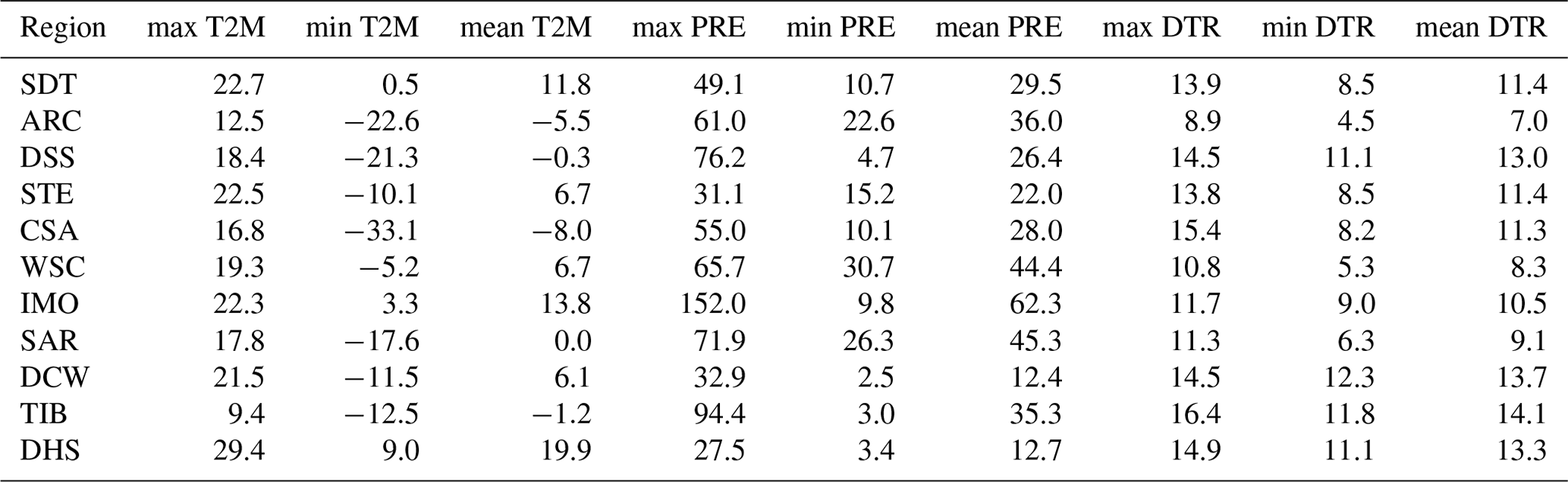
The decomposition of the domain into a set of subregions is obtained by means of a k-means clustering (Steinhaus, 1956; Ball and Hall Dj, 1965; MacQueen, 1967; Lloyd, 1982; Jain, 2010) of quantile-normalized (q-normalized) monthly climatologies of the investigated variables. K-means is a clustering technique using the concept of Euclidean distance from the centroids of a pre-determined group of clusters, for separating similar data into groups. For the purposes of this paper, following several tests and the results of other studies (Mannig et al., 2013), a total number of 11 clusters is selected. The k-means clustering algorithm is reiterated over 3000 times in order to achieve the presented results, using q-normalized values of monthly climatologies of T2M and DTR derived from the CRU data set and PRE values derived from the GPCC as input. Figure 3 shows the results of the k-means clustering. The mean climatologies of the considered regions for the three investigated variables are also reported in Table 3.
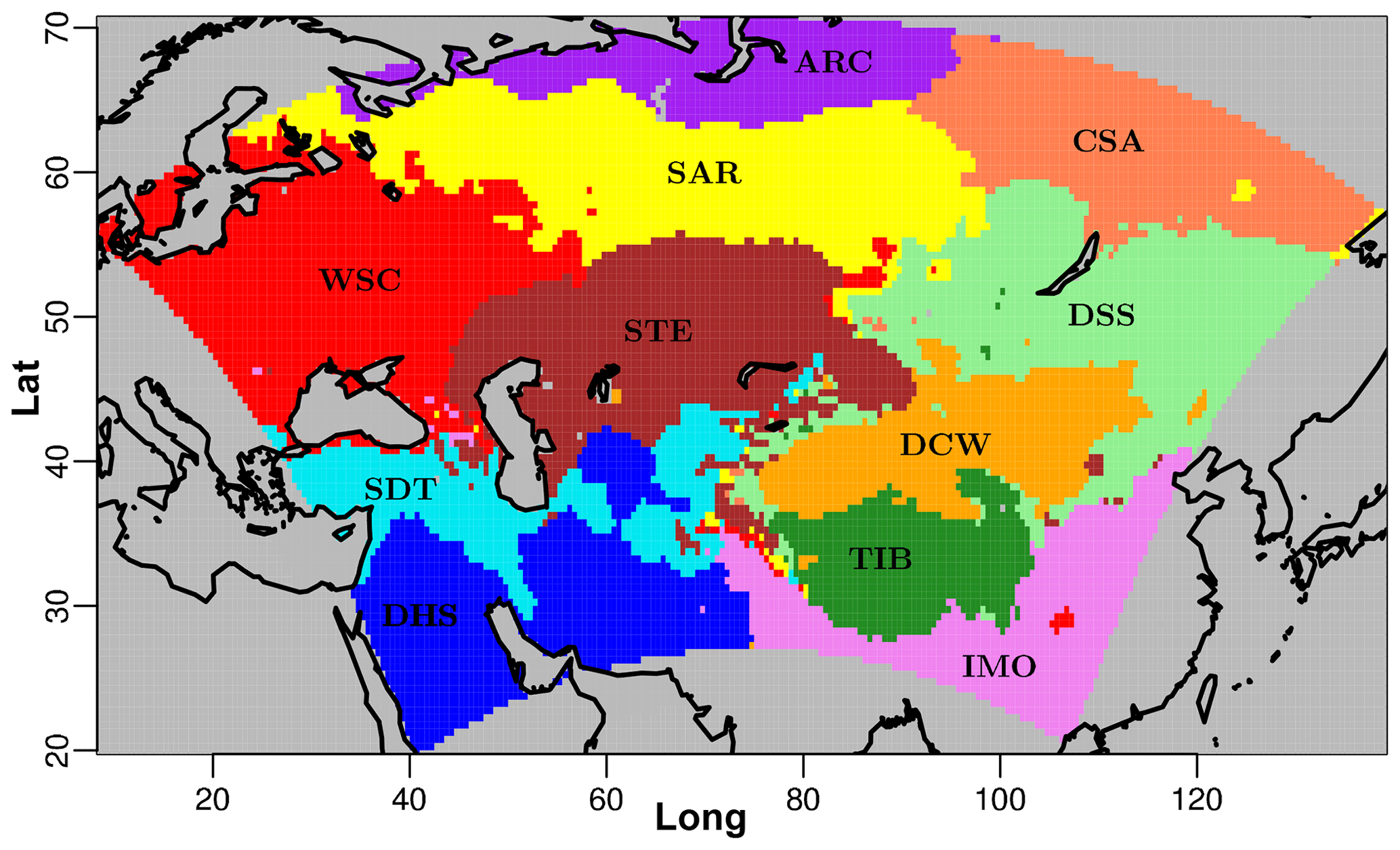
Figure 3Map of the 11 subdomains obtained through k-means clustering of the q-normalized monthly climatologies of the three considered variables over the period 1996–2005.
Table 3Subregions resulting from the k-means clustering based on climatological monthly means of near-surface temperature (T2M, CRU), precipitation (PRE, GPCC) and diurnal temperature range (DTR, CRU) for CORDEX Central Asia. Abbreviations are assigned to the different regions corresponding to their main climatic characteristics. Together with the names, mean climatic information is provided for each area. The regions illustrate the wide range of climate zones of the Central Asia domain.
For both the analyses of mean climate and variability, metrics adapted from Gleckler et al. (2008) are used. In the following subsections, we provide more details on the employed metrics.
2.3.1 Climatology
For the evaluation of the climatological means, we employ a skill score (SS) metrics expressed as
where the mean absolute error (MAE) is given by
where sim and obs are the monthly climatological means of, respectively, the considered simulation and observational data set. The indices i, j and m vary, respectively, over longitudes, latitudes and months of a year. W is the sum of the weights wijm, taking into account the different lengths of the months and the grid boxes effective area. The SS is calculated with respect to a reference simulation. Positive values indicate an improvement of the considered simulation exp with respect to the reference ref, while negative values indicate worse performance. The analyses of MAE for the mean seasonal cycle are conducted for the entire domain and single subregions. Additionally, the same metrics are applied for the analysis of single seasons for the entire area.
2.3.2 Variability
The analysis of the model performance in simulating the mean climate is complemented by the investigation of simulated variability.
There is no reason to expect models and observations to agree on the phasing of internal (unforced) variations. Hence metrics such as MAE are not appropriate for characterizing the model performance for interannual variability (Gleckler et al., 2008). Here, for an overall evaluation of the simulated variance in the different cases, the ratio of simulated to observed variance is considered
It is important to mention that correctly matching the observed variance does not guarantee correct representation of the modes of variability associated with this variance.
For taking into account observational uncertainties, all the proposed analyses are conducted separately for each observational data set. Changes in model performance for a given configuration is considered relevant only when consistent among the different observations.
In this section the results of the conducted analyses are presented, starting from the consideration of climatological means and followed by the analyses of simulated-to-observed variability.
3.1 Mean climate
In order to characterize the general performance of the model over the region, for the three considered variables, maps of the yearly, winter and summer mean biases of the reference model simulation a with respect to the different observational data sets are first presented.
Figure 4 shows that for T2M, the largest biases are evident in winter (central panels), with warmer simulated conditions over the northeastern part of the domain, where the bias in some cases exceeds 15 ∘C. These exaggerated biases are mainly relative to the UDEL data set and, in general, particularly large biases are limited to a few points characterized by complex topography and lower stations density, where the gridded data sets are less reliable. When the CRU data set is considered, the values of the bias rarely exceed (are below) 10 ∘C (−10 ∘C), for really few points. Beside these points, there are still some remarkable biases present but these are well within the ranges of other CORDEX simulations for the area (Wang et al., 2013; Bucchignani et al., 2014; Ozturk et al., 2012). In summer (Fig. 4, right panels), a positive bias (ranging from +5 to +10 ∘C) is present over the central and southwestern part of the domain, in arid and desert areas such as the Arabian Peninsula and the Taklamakan Desert. Conversely, a cold bias is present over Siberia in this case, with values rarely below −5 ∘C. Biases of annual mean values (Fig. 4, left panels) are smaller than the seasonal ones, except for the Tibetan Plateau. Here a similar particularly pronounced cold bias is evident, for all seasons, with respect to all observational data sets, with values sometimes less than −10 ∘C. In this case the observations are likely less reliable. In general, the simulation results are in better agreement with the MERRA2 data set than with the CRU and the UDEL. Nevertheless, despite the evinced differences in the magnitude of the model biases against different observational data sets, their spatial patterns are very similar in all the cases.
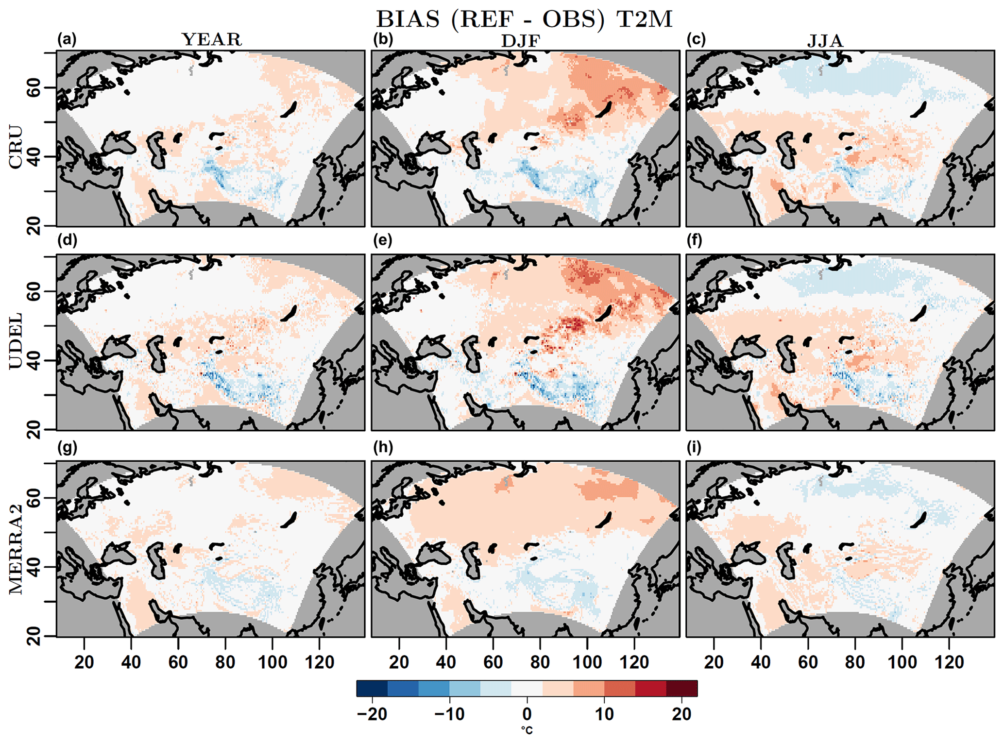
Figure 4Mean bias of annual mean (a, d, g), winter mean (b, e, h) and summer mean (c, f, i) near-surface temperature (T2M, ∘C), of the reference COSMO-CLM simulation (a) with respect to three observational data sets (from top to bottom: CRU, UDEL and MERRA2), for the period 1995–2005.
Concerning PRE (Fig. 5), remarkable biases are present in the winter and summer as well as in the annual mean for all the observational data sets. The biases in this case are expressed as a percentage with respect to the values of the corresponding observational estimates. In summer (Fig. 5, right panels), a particularly pronounced negative bias, with values down to −100 %, is visible over arid regions and the monsoon area. This is of the same order as the spread of the observational data sets for the area (Fig. 2). Over the Tibetan Plateau the bias in summer is positive, with values greater than 100 %. In winter (Fig. 5, central panels), this positive bias becomes even larger (but again of the order of the spread of observations), and extends further over adjacent regions. Over the central part of the domain, a different behavior is evident between winter and summer, while in winter the model simulates wetter conditions (+20 % to +100 %), summers are drier ( %) than in observations. In the annual mean (Fig. 5, left panels), the simulated climate is wetter over a large part of the eastern domain (with values exceeding +100 %) and drier over desert zones (with rare values smaller than −80 %). In this case, over the central part of the domain, winter and summer biases compensate each other.

Figure 5Mean bias of annual (a, d, g), winter (b, e, h) and summer mean (c, f, i) relative precipitation (PRE, %), of the reference COSMO-CLM simulation a with respect to three observational data sets (from top to bottom: CRU, UDEL and GPCC), for the period 1995–2005.
In all the cases, the simulated DTRs are smaller than the observed ones over almost the entire domain (Fig. 6). A positive bias in DTR, rarely exceeding +5 ∘C, is evident only over isolated parts of the southern domain, in particular over the southern borders of the Tibetan Plateau. The differences arising from the comparison with CRU observations are more pronounced than those with reanalysis data, with biases lower than −10 ∘C in some cases. The pattern of the bias is quite similar for all three considered data sets, with some larger differences in summer. Over the northernmost part of the domain, characterized by particularly cold conditions (minimum temperature under −30 ∘C in winter, see Table 3), a strong negative bias is evident only with respect to the CRU in all seasons. The smaller bias over this area arising from the comparison against reanalysis data is most likely due to the nature of these data sets, which combine model predictions and observations.
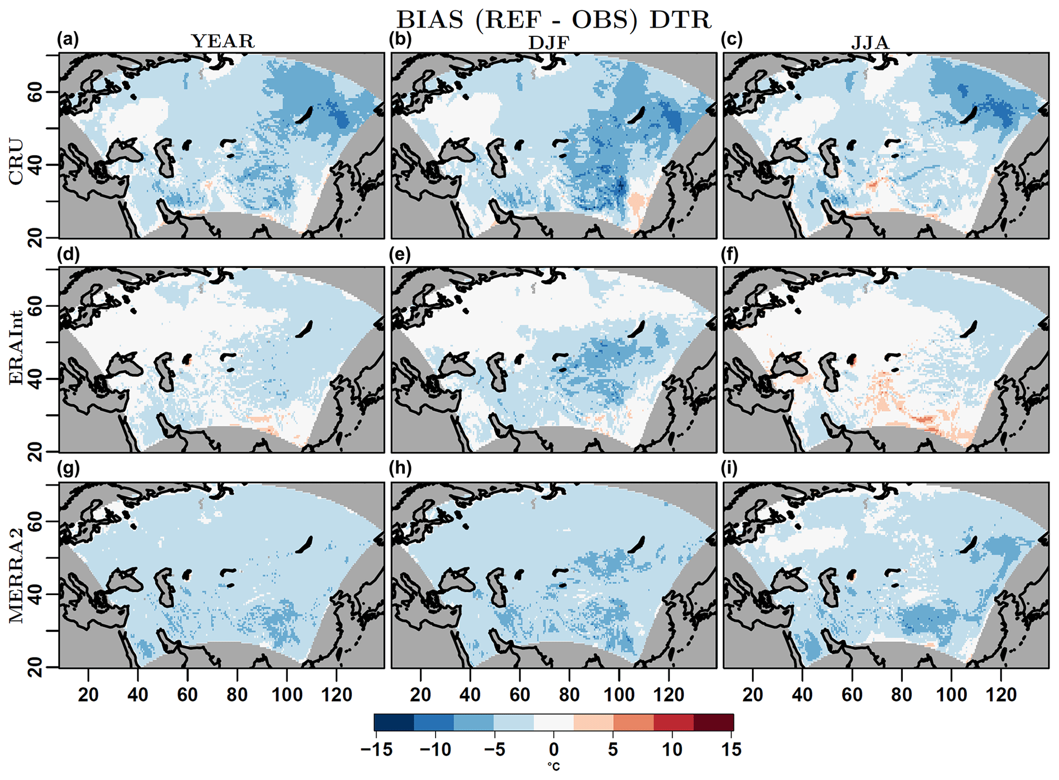
Figure 6Mean bias of annual (a, d, g), winter (b, e, h) and summer mean (c, f, i) diurnal temperature range (DTR, ∘C), of the reference COSMO-CLM simulation a with respect to three observational data sets (from top to bottom: CRU, MERRA2 and ERA-Interim), for the period 1995–2005.
The additional simulations performed with the same reference setup but with a different time step (TIMESTEP, Table 1) and driven by ERA-Interim instead of NCEP2 (a_ERA-Interim, Table 1), lead to very similar biases, for all variables (see Supplement). This suggests that evinced biases are likely inherent to the model formulation itself.
3.1.1 SS – seasonal cycle
In this section, the results of the skill score (SS) derived from the MAE calculated over the mean seasonal cycle and all the points of the domain are presented.
Figure 7a shows that for T2M, among the experiments for which single changes are applied to the reference model configuration (left side of the dotted vertical line), those with changes in the albedo treatment (c+d) lead to a noticeable improvement of the results (ranging between +4.5 % and +7 %). Nevertheless, in this case, the largest improvements (greater than 5 % for all the observational data sets) are obtained for experiment j, in which the type of the hydraulic lower boundary accounts for ground water with drainage and diffusion. Combining the configuration changes of different experiments (right side of Fig. 7) the results for temperature are considerably improved whenever either one of the setup changes of experiments d or j are used, with values of SS larger than 4 % in almost all the cases. Other “combined” experiments do not have an important effect on the results.
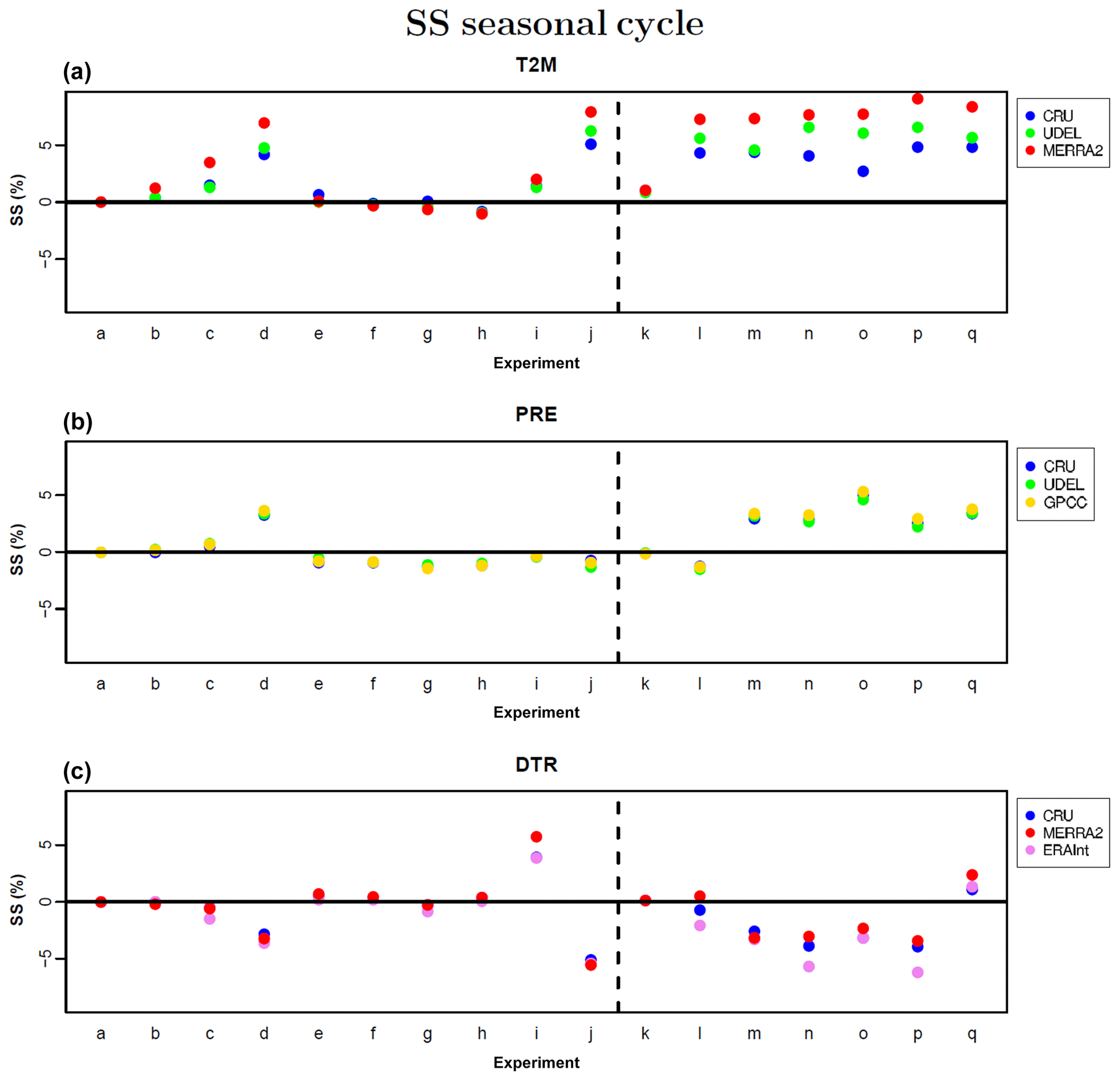
Figure 7Skill score (SS) derived from the MAE calculated over the monthly climatological values of the seasonal cycle of different COSMO-CLM simulations and observational data sets. From top to bottom, the SS for near-surface temperature (T2M), precipitation (PRE) and diurnal temperature range (DTR) is respectively displayed. The dotted vertical black line divides the simulations with the same configuration of the reference simulation plus a single change in the model setup (left) and those obtained through the combinations of the previous ones (right). Positive (negative) values indicate better (worse) performance of the considered simulations compared to the reference one.
For PRE (Fig. 7b), only the results of one experiment, among those with single changes in the model configuration, are improved compared to the reference: experiment d (SS %), in which the albedo is modified considering the forest fraction. The positive effect of this change is slightly enhanced when used jointly with other configuration choices (experiments m, n, o, p, q), having indeed an important effect on precipitation.
As for PRE, also for DTR (Fig. 7c) only one experiment seems to sensibly improve over the results of the reference simulation: experiment i (SS ranging between +4 % and +5 %). In this experiment, the soil heat conductivity takes into account the ratio of soil moisture to soil ice. For DTR two experiments, d and j, lead to particularly negative skills (SS between −4 % and −5 %), which also affect the combined experiments including their configuration changes. The unique exception is the combined experiment q in this case: the negative effects on the simulation of DTR of experiment d seem to be compensated by the positive ones of experiment i, resulting in positive values of SS, varying between +1 % and +2 %.
In summary, the presented analyses show that the combined representation of surface albedo (taking into account forest fraction) and soil heat conductivity (accounting for the ratio between ice and moisture in the soil), as configured in experiment q, has the best positive effects on the representation of the mean seasonal cycle of all three considered variables, among all the tested configurations.
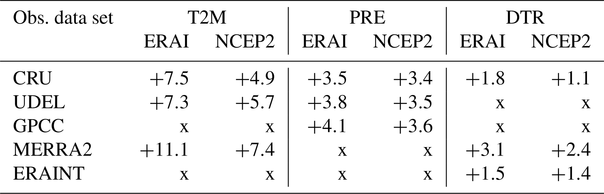
Although some differences in the results of the SS calculated based on the different observational data sets are evident, experiment q shows the same positive sign of improvement in all the cases. This is also true when comparing the results obtained driving the same simulations q and a with NCEP2 and ERA-Interim reanalysis data (Table 4). This confirms the potential of experiment q in improving model performance for the area.
Table 4Changes of the SS calculated for experiment q with respect to reference simulation a, when both simulations are driven by ERA-Interim (left) and NCEP2 (right) reanalysis data.
3.1.2 SS – subdomains
The same SS analyses for the mean seasonal cycle are conducted for subregions characterized by similar climate conditions. This allows one to test the model sensitivity for regions where different physical processes might play a different role. The analyses presented in Fig. 8 are conducted, as in the case of the entire domain, separately for different observational data sets. Here, for visualization reasons, the magnitude of changes in the SS is only reported for a reference data set for each variable, being the CRU for T2M and DTR and the GPCC for PRE. At the same time, for each experiment and subregion where the sign of changes in SS is the same among the different observations, a point is drawn.
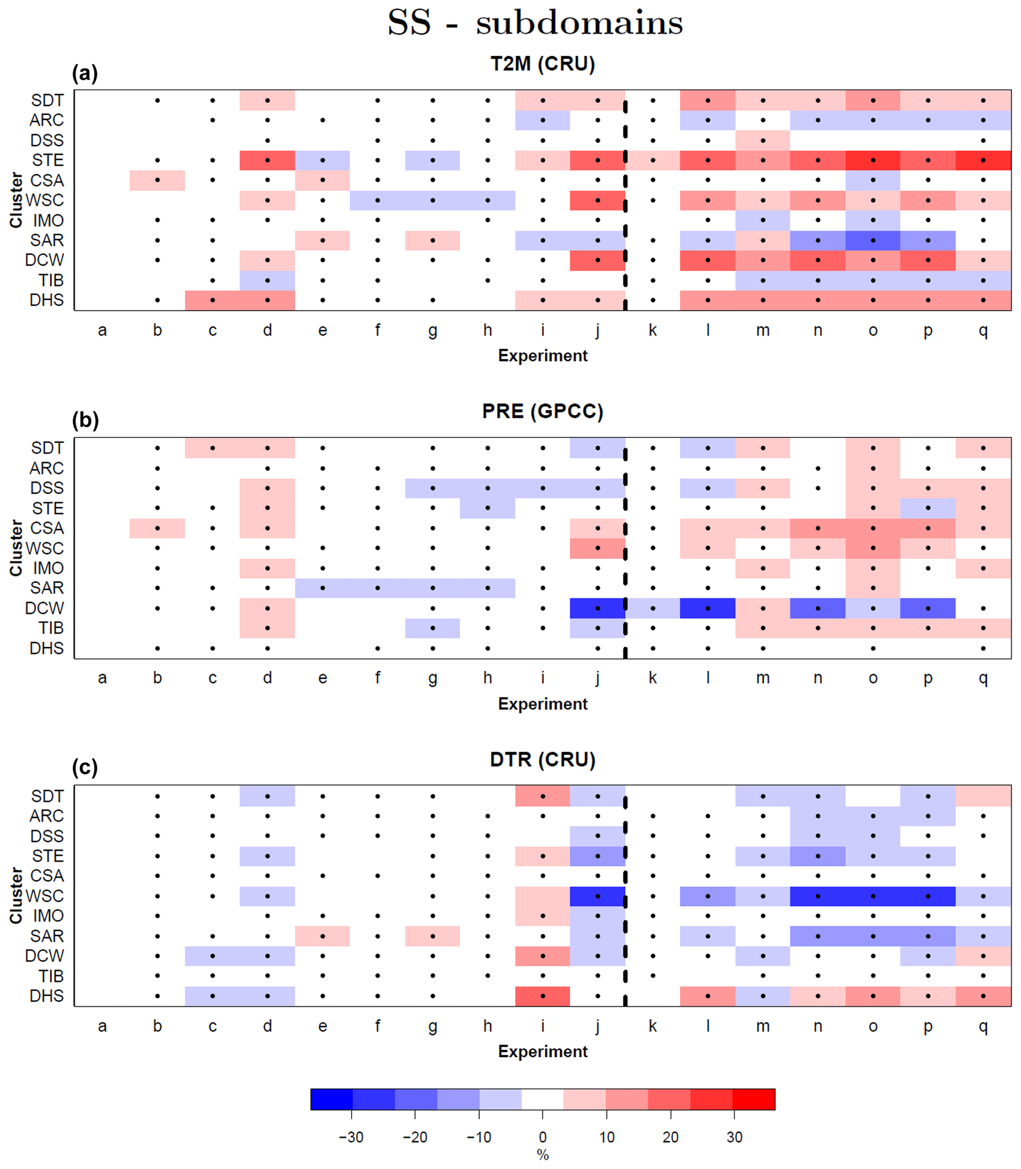
Figure 8Skill score (SS) derived from the MAE calculated for each domain subregion over the monthly climatological values of the seasonal cycle of different COSMO-CLM simulations and observational data sets. From top to bottom, each panel represents the results obtained for near-surface temperature (T2M) using the CRU, for precipitation (PRE) using the GPCC and for diurnal temperature range (DTR) using the CRU as observational data sets. Positive (negative) values indicate better (worse) performance of the considered simulations compared to the reference one. The points in correspondence of different clusters and experiments indicate that the change is the SS is the same in sign among the three observational data sets considered for each variable.
Figure 8 basically confirms the results of the SS calculated for the entire domain. For the experiments with single changes in the reference model configuration it is possible to see that for T2M (upper panel), the most relevant SS changes are obtained for experiment d and j, with improvements exceeding 30 % over a given region. For PRE (middle panel), improvements over all the clusters are obtained only for experiment d, and positive SS values are evident only for a few other experiments for specific subdomains. In this case, changes in SS are smaller than for T2M, rarely exceeding 10 %. For DTR, experiment i allows one to improve model performance by up to 25 % with respect to the reference simulation, not visible in the other cases, for almost all the subdomains.
Among the combined experiments (right side of each panel of Fig. 8), it is possible to affirm that experiments m and q present similar performance for T2M and PRE. Conversely, only experiment q shows an important improvement in model performance on more than one subdomain for DTR.
Figure 8 shows that it is almost impossible to achieve an improvement in model performance for all regions and variables. Despite experiment q presenting positive SS values for a large majority of subdomains, some negative values are also evident for specific subregions. This also happens when considering different variables. For example, for experiment d, improvements over the entire domain are evident for T2M and PRE, while the same setup leads to worse model performance in terms of DTR, for almost the entire domain. Therefore, even though important improvements are obtained in different cases, it is crucial to highlight the fact that these might be the product of a compensation effect over different variables and domain subregions.
3.1.3 SS – single seasons
The same SS analyses are additionally conducted for the monthly climatologies of each season, over the entire domain. Seasonal analyses could help in determining simulations presenting good and coherent performance over more periods of the year. The results, reported in the Supplement of this paper, show that the largest changes in the seasonal values of SS are obtained for summer, for processes related to the representation of surface and soil properties. On the other hand, in winter the changes in model performance among the different experiments are substantially smaller than in the other seasons. Overall, for single seasons, the most important and consistent improvements in the simulated climatological mean of the considered variables with respect to the reference simulation are obtained for experiment q, confirming the results obtained for the seasonal cycle.
3.1.4 Effects of soil depth and snow model on mean winter temperatures
The two simulations (SOIL and SNOW) specifically designed for testing the effects of changes in soil depth and the use of a multi-layer snow model on the COSMO-CLM simulation of T2M over areas characterized by the presence of permafrost and snow in winter do not present significantly different results than the reference simulation (Fig. 9). In particular, they do not allow one to reduce the warm bias in T2M present for the reference simulation in winter over the western Siberia part of the domain, with even warmer conditions simulated by experiment SNOW (Fig. 9, left).
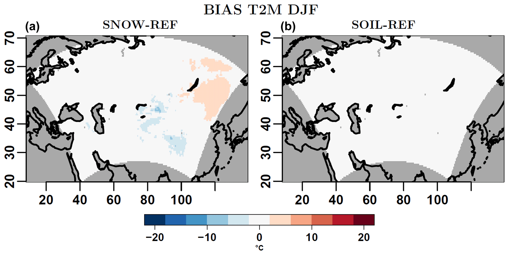
Figure 9Near-surface temperature (T2M, ∘C) winter mean bias calculated with respect to the reference simulation over the period 2006–2015, for the simulations SNOW (a) and SOIL (b).
3.2 Variability
In this section, the results of the analysis of simulated variance is presented, with the goal of complementing the analyses of the mean climate of Sect. 3.1. First, a general overview of the model skill in simulating observational variability is described, followed by a discussion of the different uncertainties affecting this metrics.
Figure 10 shows the ratio of variance of the different COSMO-CLM experiments with respect to that of the observations. The variances are calculated from monthly anomaly values of the three considered variables averaged over the subregions shown in Fig. 3 (see also Sect. 2.3). For visualization reasons, a single observational data set is used for each of the considered variables in this case: CRU for T2M and DTR, and GPCC for PRE. The results of the comparison against other observational data sets are considered when discussing different sources of uncertainties in Sect. 3.2.1.
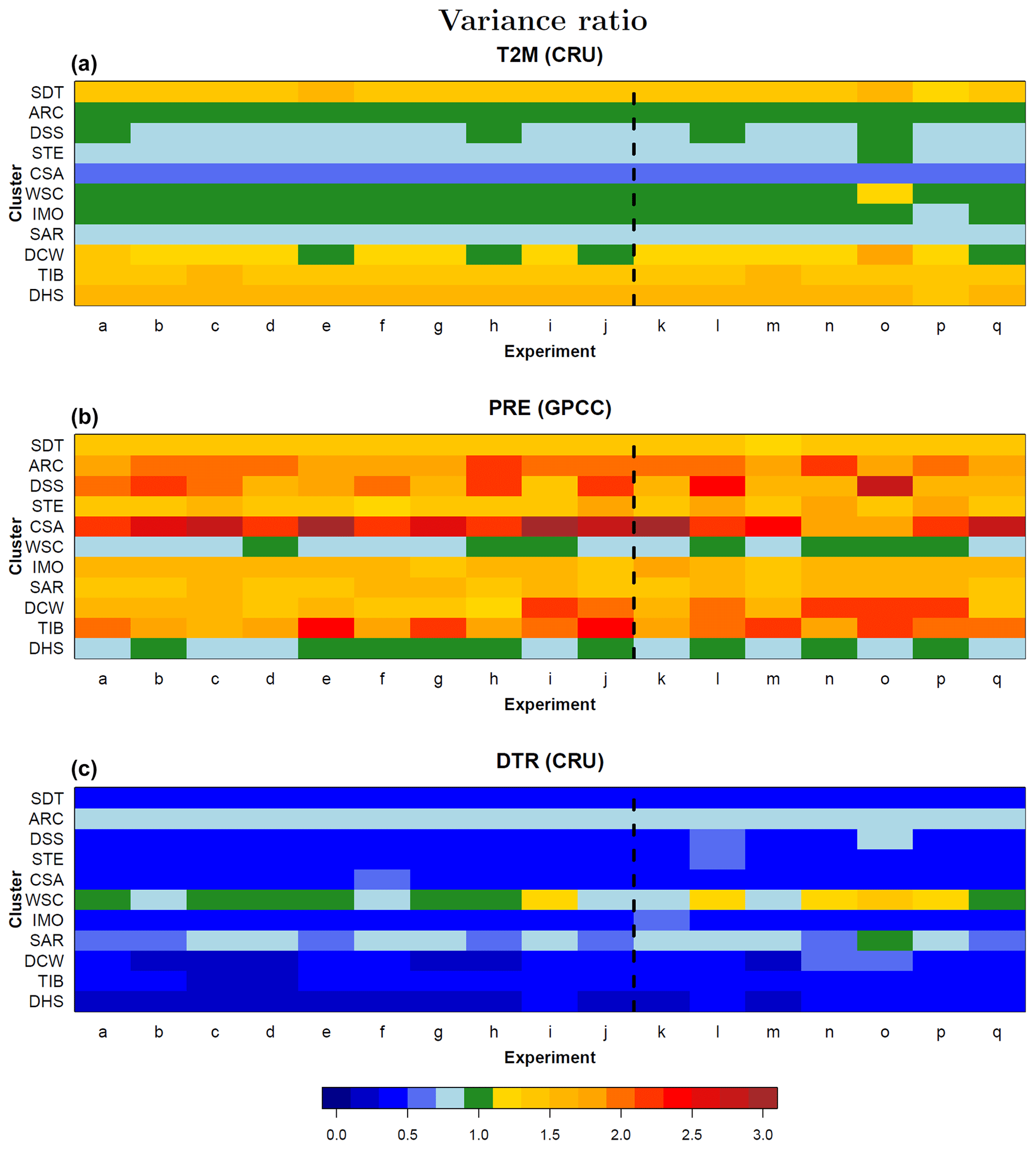
Figure 10Fraction of variance calculated between the monthly anomalies over the period 1996–2005 derived from the different COSMO-CLM simulations and a single observational data set, for (top to bottom) near-surface temperature (T2M) using the CRU, precipitation (PRE) using the GPCC and diurnal temperature range (DTR) using the CRU as observational data sets, for each of the 11 subregions obtained by k-means clustering. The dotted vertical black line divides the simulations with the same configuration of the reference simulation plus a single change in the model setup (left) and those obtained through the combinations of the previous ones (right). Values of more (less) than 1 indicate better (worse) performance of the considered simulations with respect to the reference one, in the representation of observed variability.
In general, for DTR and T2M, there are no large differences in the variance ratios of all the experiments, except for a few subregions. For PRE, conditions are more heterogeneous, with relatively large differences among all the simulations. Nevertheless, the most pronounced changes are still limited to a few clusters.
For T2M, the best results in terms of simulated variance are obtained: the model is able to reproduce the interannual variability of the observations particularly well. In particular, a good agreement between simulated data and observations is evident for subregions WSC, IMO and ARC. The largest underestimation of the observed variance of T2M is obtained for cluster CSA. Therefore, the model is not only unable to simulate the mean temperatures of particularly cold areas, as demonstrated in Sect. 3.1, but it also shows a very low variability for the same variable, over these regions, when compared to observations. A particularly small value of the variance ratio is also evident for T2M for the subdomains DSS, SAR and STE throughout almost all the experiments. These regions are all characterized by a large range between minimum and maximum monthly temperatures (see Table 3).
For PRE, in general, the values of the ratio of simulated-to-observed variance are considerably greater than 1 for almost all the experiments and subdomains. Values are closer to 1 only for the domains WSC and DHS throughout all the experiments. In the domains CSA, DSS and TIB, variance ratios are particularly remarkable, reaching a value of 3 for a given experiment. Over these domains, characterized by complex topography, the results from Sect. 3.1 have shown that the model simulates significantly wetter conditions. Hence, for mountainous areas of the domain the model overestimates both mean values and variability of precipitation.
Values of variance ratios for DTR are smaller than 1 over almost all the subdomains and simulations. This indicates that the model, beside underestimating climatological values of the observed temperature diurnal cycle over the entire Central Asia domain as demonstrated in Sect. 3.1, also underestimates the amplitude of variations in the monthly means.
3.2.1 Uncertainties in the investigation of simulated variability
In this section, the influence of uncertainties associated with the observational data sets, boundary data and internal variability on the evaluation of simulated variability are quantified. To investigate the effect of the model internal variability, four additional simulations have been conducted using the setup of the reference simulation, but shifting the initial date by ±1 and ±3 months.
The left columns of each panel of Fig. 11 show the absolute differences in the variance ratio of experiment a calculated, for each variable, with respect to different observational data sets. In addition, the right columns of the same figure show the absolute differences in the variance ratio between experiment a and the other experiments. The range of changes in the two cases is comparable for almost all clusters and variables. In many cases, the changes resulting from the use of different observations are larger than the differences between the experiments. In these cases, the observational uncertainty is thus too large to allow for a classification of the different experiments in terms of their skill in reproducing the observed variance. The influence of the observational data sets on the variance ratios is larger for PRE and DTR than for T2M.

Figure 11Absolute differences in variance ratio. The left column of each panel shows the absolute differences in the variance ratio of the same experiment, a, when considering different observational data sets. The right column of each panel shows the range of absolute differences between the variance ratio of experiment a and that of the other experiments, from b to q, when using a single observational data set for each variable. From left to right, the panels respectively present the results of the comparison for near-surface temperature (T2M), precipitation (PRE) and diurnal temperature range (DTR). The different rows show the results obtained for each of the clusters.
Despite the fact that variations in the boundary data and in the simulated internal variability (as quantified in the additional experiments with shifted initial dates) do not have the same strong effect on the simulated variance ratio as the observational uncertainties, for some regions their values are still comparable to the differences between the simulations (not shown).
In conclusion, the fact that different uncertainties are of the same order of magnitude as the differences between the simulations prevents a classification of the different experiments with respect to their skill in representing the observed variability.
The main goal of this work is to evaluate a set of different configuration setups of the regional climate model COSMO-CLM over the CORDEX Central Asia domain, and to isolate different sources of uncertainties, in order to quantify general model performance and to provide a basis for possible improvements of the model simulations for this region. The results of this study are of fundamental importance in the light of the next phase of the CORDEX initiative, in particular considering the vulnerability of the region to the possible effects of climate change.
Concerning the simulation of the mean climate, the model shows remarkable deficiencies in simulating the three considered variables (near-surface temperature, precipitation and diurnal temperature range) over different areas of Central Asia and different seasons. Even though over specific areas of the domain these biases are hard to be quantitatively assessed, due to high uncertainties in the considered observational data sets, their spatial pattern is similar in all the cases.
For temperature, large positive model biases are present in winter over Siberia, with remarkable values exceeding +10 ∘C in some cases. There are two likely reasons for these biases: unsatisfactory representation of snow cover and of soil permafrost. In fact, both these factors have a significant impact on heat transport within the soil and heat flux between soil and atmosphere, with important effects on near-surface temperatures (Frauenfeld et al., 2004; Lachenbruch and Marshall, 1986; Saito et al., 2007; Klehmet, 2014). Siberian permafrost often exceeds a depth of 100 m, reaching values of up to 1 km (Yershov, 2004). Therefore, many studies (Alexeev et al., 2007; Dankers et al., 2011; Nicolsky et al., 2007; Lawrence et al., 2008; Saito et al., 2007; Klehmet, 2014) highlight the importance of an adequate depth of model soil layers for the proper representation of processes related to permafrost. At the same time, other studies (Saito et al., 2007; Waliser et al., 2011; Klehmet, 2014) suggest that a better representation of the vertical stratification of the snow pack could have a significant effect on the simulated energy budget and, consequently, on near-surface temperatures over the area. Following these hypotheses, two additional, 25-year simulations have been conducted during this study, with an increase of the total model soil depth and with the use of a multi-layer snow model. Results indicate that, for the part of Siberia included in the domain of study, no significant changes are evident in the two cases. This further demarcates model limitations, pointing to a structural problem in the model formulation and to the need for new parameterizations for the simulation of processes related to snow cover and permafrost in COSMO-CLM. Importantly, an additional cold bias, in some cases lower than −10 ∘C, is present for every season over the Tibetan Plateau. Other regional climate models suffer from a similar bias (Guo et al., 2018; Meng et al., 2018). Acknowledging the fact that for this area the observational uncertainty is particularly high, the evinced biases could partly be related to a bad representation of the albedo for highly complex topographies. In fact, a study by Meng et al. (2018) showed that changes in the albedo over the region have led to an important improvement of the results of an RCM. Another possible explanation for this cold bias might be the parametrization of surface fluxes (Zhuo et al., 2016). Consequently, further analyses should focus on improving the mode representation of these processes.
For precipitation, particularly wet conditions are simulated by the COSMO-CLM over the Tibetan Plateau. This bias seems to be common to several RCMs for areas characterized by complex topography (Guo et al., 2018; Gao et al., 2015; Feng and Fu, 2006) and is likely related to an overestimation of orographic precipitation enhancement in the models (Gerber et al., 2018) and/or to an incorrect simulation of the planetary boundary layer (Xu et al., 2016). Additionally, in the COSMO-CLM simulations a significant dry bias occurs over arid and desert regions, especially in summer. A similar COSMO-CLM bias has already been seen for other semi-arid and dry regions of the world, such as the Mediterranean region. In this case, it was connected with an incorrect simulation of soil–atmosphere interactions by the model (Fischer et al., 2007; Seneviratne et al., 2010; Russo and Cubasch, 2016), which is likely the case also for Central Asia. For both the Tibetan Plateau and arid summer areas, it is important to note that the biases are of the same order of the spread of the observations.
The model underestimates the climatological mean of the diurnal cycle of temperatures, for all the seasons and subregions of the domain. This bias is relatively homogeneous over the entire domain of study. Several studies have shown that RCMs typically underestimate diurnal temperature ranges over different parts of the world (Kyselỳ and Plavcová, 2012; Mearns et al., 1995; Laprise et al., 2003). The main factors responsible for these deficiencies seem to be errors in the simulation of the atmospheric circulation, cloud cover and heat and moisture fluxes between surface and atmosphere.
The evinced model limitations for the mean climate do not seem to differ significantly when considering ERA-Interim as driving data and a different time step.
In order to test whether it is possible to reduce the determined model biases, and to which degree, sensitivity experiments have been performed to study the effect of different changes in the configuration of COSMO-CLM and their mutual interaction. After considering different sources of uncertainties, the combined change of the albedo, taking into consideration the ratio of forest fractions, and the soil conductivity, taking into account the ratio of liquid water and ice in the soil, leads to the best results in simulated climatological means of the three considered variables (experiment q). Importantly, the model seems to be particularly sensitive to those parameterizations that deal with soil and surface features, and that could positively affect the repartition of incoming radiation.
An analysis of model performance in simulating climatological means per subregions characterized by similar physical processes shows that different model configurations may lead to improvements exceeding 30 % over a given region. The analysis for subregions is coherent with the SS analyses conducted over the entire domain, with experiment q presenting the best performance over the largest majority of regions, for all variables, in the two cases. Nevertheless, subregion analyses show that improvements in model performance are not homogeneous among all the subregions and variables, but they are the result of a given compensation effect in the different cases.
The investigation of model performance for the simulation of seasonal climatologies confirms the results obtained for the seasonal cycle, with experiment q leading to the best and most consistent results among all the seasons. For all the analyzed variables, winter is the season for which no substantial improvements in model results can be achieved with the set of investigated configurations. This suggests that other factors, playing a crucial role in the simulation of Central Asia winter climate, are not properly considered in COSMO-CLM.
The model improvements in the simulation of climatological means, with the same optimal configuration, are very similar when considering different observational data sets, and ERA-Interim instead of NCEP2 as drivers.
Finally, the observed variability of temperature is relatively well represented in the model simulations for different subregions of the domain. For precipitation, the model overestimates the variability of observations. On the contrary, the model underestimates the variability in the diurnal cycle of temperatures over the entire region. Among the three investigated variables, only for precipitation are there significant changes in the simulated variance throughout all conducted experiments. However, due to the large uncertainties in the variability estimates from observations, the use of different boundaries and the model internal variability, it has not been possible to rank the different simulations according to their representation of monthly variability.
All the data upon which this research is based are available through personal communication with the authors. The codes used for the postprocessing of model results are available at the following links: https://doi.org/10.5281/zenodo.3469945 (Russo, 2019a), https://doi.org/10.5281/zenodo.3516622 (Russo, 2019b).
The model configuration files of the performed sensitivity tests can be reviewed at: https://doi.org/10.5281/zenodo.3516676 (Russo, 2019c).
The data derived from the model outputs and on which all the presented analyses are based, can be downloaded at: https://doi.org/10.5281/zenodo.3516708 (Russo, 2019d).
The supplement related to this article is available online at: https://doi.org/10.5194/gmd-12-5229-2019-supplement.
The simulations of this research were performed by ER. All the authors equally contributed to the discussion of the results. The paper structure and most of the presented experiments were designed by ER and IK. All authors substantially contributed to the revision of the text and to the formatting of the paper.
The authors declare that they have no conflict of interest.
The computational resources necessary for conducting the experiments presented in this research were made available by the German Climate Computing Center (DKRZ).
The authors are also particularly grateful to the CLM community for all their efforts in developing COSMO-CLM and making its code available.
This study was funded by the Federal Ministry of Education and Research of
Germany (BMBF) as part of the CAME II project (Central Asia: Climatic Tipping
Points & Their Consequences), project no. 03G0863G.
We acknowledge support
from the Open Access Publication
Initiative of Freie
Universität Berlin.
This paper was edited by Leena Järvi and reviewed by two anonymous referees.
Airey, M. and Hulme, M.: Evaluating climate model simulations of precipitation: methods, problems and performance, Prog. Phys. Geog., 19, 427–448, 1995. a
Alexeev, V., Nicolsky, D., Romanovsky, V., and Lawrence, D.: An evaluation of deep soil configurations in the CLM3 for improved representation of permafrost, Geophys. Res. Lett., 34, L09502, https://doi.org/10.1029/2007GL029536, 2007. a
Avgoustoglou, E., Voudouri, A., Khain, P., Grazzini, F., and Bettems, J.: Design and Evaluation of Sensitivity Tests of COSMO Model Over the Mediterranean Area, in: Perspectives on Atmospheric Sciences, Springer, 49–54, 2017. a
Awan, N., Truhetz, H., and Gobiet, A.: Parameterization-induced error characteristics of MM5 and WRF operated in climate mode over the Alpine region: an ensemble-based analysis, J. Climate, 24, 3107–3123, 2011. a
Bachner, S., Kapala, A., and Simmer, C.: Evaluation of daily precipitation characteristics in the CLM and their sensitivity to parameterizations, Meteorol. Z., 17, 407–419, 2008. a
Ball, G. and Hall Dj, I.: A novel method of data analysis and pattern classification, Isodata, A novel method of data analysis and pattern classification, Tch. Report 5RI, Project 5533, 1965. a
Bechtold, P., Köhler, M., Jung, T., Doblas-Reyes, F., Leutbecher, M., Rodwell, M., Vitart, F., and Balsamo, G.: Advances in simulating atmospheric variability with the ECMWF model: From synoptic to decadal time-scales, Q. J. Roy. Meteor. Soc., 134, 1337–1351, 2008. a
Becker, A., Finger, P., Meyer-Christoffer, A., Rudolf, B., and Ziese, M.: GPCC Full Data Reanalysis Version 7.0: Monthly Land-Surface Precipitation from Rain Gauges built on GTS based and Historic Data. Research Data Archive at the National Center for Atmospheric Research, Computational and Information Systems Laboratory, https://doi.org/10.5065/D6000072, 2011. a
Bellprat, O., Kotlarski, S., Lüthi, D., and Schär, C.: Exploring perturbed physics ensembles in a regional climate model, J. Climate, 25, 4582–4599, 2012a. a, b, c
Bellprat, O., Kotlarski, S., Lüthi, D., and Schär, C.: Objective calibration of regional climate models, J. Geophys. Res.-Atmos., 117, D23115, https://doi.org/10.1029/2012JD018262, 2012b. a, b, c, d
Bellprat, O., Kotlarski, S., Lüthi, D., De Elía, R., Frigon, A., Laprise, R., and Schär, C.: Objective calibration of regional climate models: application over Europe and North America, J. Climate, 29, 819–838, 2016. a
Bentsen, M., Bethke, I., Debernard, J. B., Iversen, T., Kirkevåg, A., Seland, Ø., Drange, H., Roelandt, C., Seierstad, I. A., Hoose, C., and Kristjánsson, J. E.: The Norwegian Earth System Model, NorESM1-M – Part 1: Description and basic evaluation of the physical climate, Geosci. Model Dev., 6, 687–720, https://doi.org/10.5194/gmd-6-687-2013, 2013. a
Borge, R., Alexandrov, V., Del Vas, J., Lumbreras, J., and Rodriguez, E.: A comprehensive sensitivity analysis of the WRF model for air quality applications over the Iberian Peninsula, Atmos. Environ., 42, 8560–8574, 2008. a
Bucchignani, E., Mercogliano, P., Montesarchio, M., Zollo, A., and Manzi, M.: Prearrangement of the COSMO-CLM Model on the Chinese region and sensitivity analysis, CMCC Research Paper, 2012. a
Bucchignani, E., Montesarchio, M., Cattaneo, L., Manzi, M. P., and Mercogliano, P.: Regional climate modeling over China with COSMO-CLM: Performance assessment and climate projections, J. Geophys. Res.-Atmos., 119, 12–151, 2014. a, b
Bucchignani, E., Cattaneo, L., Panitz, H., and Mercogliano, P.: Sensitivity analysis with the regional climate model COSMO-CLM over the CORDEX-MENA domain, Meteorol. Atmos. Phys., 128, 73–95, 2016. a, b
Chuluunkhuyag, S.: The impact of climate change and human activity on Mongolian water resources, in: International water conference paper, 2008. a
Collins, M., AchutaRao, K., Ashok, K., Bhandari, S., Mitra, A., Prakash, S., Srivastava, R., and Turner, A.: Observational challenges in evaluating climate models, Nat. Clim. Change, 3, 940–941, https://doi.org/10.1038/nclimate2012, 2013. a
Crétat, J., Pohl, B., Richard, Y., and Drobinski, P.: Uncertainties in simulating regional climate of Southern Africa: sensitivity to physical parameterizations using WRF, Clim. Dynam., 38, 613–634, 2012. a
Dankers, R., Burke, E. J., and Price, J.: Simulation of permafrost and seasonal thaw depth in the JULES land surface scheme, The Cryosphere, 5, 773–790, https://doi.org/10.5194/tc-5-773-2011, 2011. a
Davies, H.: A lateral boundary formulation for multi-level prediction models, Q. J. Roy. Meteor. Soc., 102, 405–418, 1976. a
Dee, D. P., Uppala, S. M., Simmons, A. J., Berrisford, P., Poli, P., Kobayashi, S., Andrae, U., Balmaseda, M. A., Balsamo, G., Bauer, P., Bechtold, P., Beljaars, A. C. M., van de Berg, L., Bidlot, J., Bormann, N., Delsol, C., Dragani, R., Fuentes, M., Geer, A. J., Haimberger, L., Healy, S. B., Hersbach, H., Hólm, E. V., Isaksen, L., Kållberg, P., Köhler, M., Matricardi, M., McNally, A. P., Monge-Sanz, B. M., Morcrette, J.-J., Park, B.-K., Peubey, C., de Rosnay, P., Tavolato, C., Thépaut, J.-N., and Vitart, F.: The ERA-Interim reanalysis: Configuration and performance of the data assimilation system, Q. J. Roy. Meteor. Soc., 137, 553–597, 2011. a, b
de Elía, R., Caya, D., Côté, H., Frigon, A., Biner, S., Giguère, M., Paquin, D., Harvey, R., and Plummer, D.: Evaluation of uncertainties in the CRCM-simulated North American climate, Clim. Dynam., 30, 113–132, 2008. a
Diniega, R.: The Effect of Climate Change on Mongolian Herding Communities: Investigating the Current Prevalence of Ecomigration and Community Perceptions of and Responses to Migration in the Countryside, 2012. a
Diro, G., Rauscher, S., Giorgi, F., and Tompkins, A.: Sensitivity of seasonal climate and diurnal precipitation over Central America to land and sea surface schemes in RegCM4, Clim. Res., 52, 31–48, 2012. a
Dobler, A. and Ahrens, B.: Analysis of the Indian summer monsoon system in the regional climate model COSMO-CLM, J. Geophys. Res.-Atmos., 115, D16101, https://doi.org/10.1029/2009JD013497, 2010. a
Dong, S. and Sun, Y.: Comparisons of observational data sets for evaluating the CMIP5 precipitation extreme simulations over Asia, Clim. Res., 76, 161–176, 2018. a
Evans, J., Ekström, M., and Ji, F.: Evaluating the performance of a WRF physics ensemble over South-East Australia, Clim. Dynam., 39, 1241–1258, 2012. a
Feng, J. and Fu, C.: Inter-comparison of 10-year precipitation simulated by several RCMs for Asia, Adv. Atmos. Sci., 23, 531–542, 2006. a
Fernández, J., Montávez, J., Sáenz, J., González-Rouco, J., and Zorita, E.: Sensitivity of the MM5 mesoscale model to physical parameterizations for regional climate studies: Annual cycle, J. Geophys. Res.-Atmos., 112, D04101, https://doi.org/10.1029/2005JD006649, 2007. a
Fischer, E., Seneviratne, S., Lüthi, D., and Schär, C.: Contribution of land-atmosphere coupling to recent European summer heat waves, Geophys. Res. Lett., 34, L06707, https://doi.org/10.1029/2006GL029068, 2007. a
Flaounas, E., Drobinski, P., Borga, M., Calvet, J., Delrieu, G., Morin, E., Tartari, G., and Toffolon, R.: Assessment of gridded observations used for climate model validation in the Mediterranean region: the HyMeX and MED-CORDEX framework, Environ. Res. Lett., 7, 024017, https://doi.org/10.1088/1748-9326/7/2/024017, 2012. a, b
Flato, G., Marotzke, J., Abiodun, B., Braconnot, P., Chou, S. C., Collins, W. J., Cox, P., Driouech, F., Emori, S., Eyring, V., Forest, C., Gleckler, P., Guilyardi, E., Jakob, C., Kattsov, V., Reason, C., and Rummukainen, M.: Evaluation of climate models. In: climate change 2013: the physical science basis. Contribution of working group I to the fifth assessment report of the intergovernmental panel on climate change, Climate Change, 5, 741–866, 2013. a
Frauenfeld, O., Zhang, T., Barry, R., and Gilichinsky, D.: Interdecadal changes in seasonal freeze and thaw depths in Russia, J. Geophys. Res.-Atmos., 109, D05101, https://doi.org/10.1029/2003JD004245, 2004. a
Gao, Y., Xu, J., and Chen, D.: Evaluation of WRF mesoscale climate simulations over the Tibetan Plateau during 1979–2011, J. Climate, 28, 2823–2841, 2015. a
García-Díez, M., Fernández, J., Fita, L., and Yagüe, C.: Seasonal dependence of WRF model biases and sensitivity to PBL schemes over Europe, Q. J. Roy. Meteor. Soc., 139, 501–514, 2013. a
Gelaro, R., McCarty, W., Suárez, M., Todling, R., Molod, A., Takacs, L., Randles, C., Darmenov, A., Bosilovich, M., Reichle, R., Wargan, K., Coy, L., Cullather, R., Draper, C., Akella, S., Buchard, V., Conaty, A., da Silva, A. M., Gu, W., Kim, G., Koster, R., Lucchesi, R., Merkova, D., Nielsen, J. E., Partyka, G., Pawson, S., Putman, W., Rienecker, M., Schubert, S. D., Sienkiewicz, M., and Zhao, B.: The modern-era retrospective analysis for research and applications, version 2 (MERRA-2), J. Climate, 30, 5419–5454, 2017. a
Gerber, F., Besic, N., Sharma, V., Mott, R., Daniels, M., Gabella, M., Berne, A., Germann, U., and Lehning, M.: Spatial variability in snow precipitation and accumulation in COSMO–WRF simulations and radar estimations over complex terrain, The Cryosphere, 12, 3137–3160, https://doi.org/10.5194/tc-12-3137-2018, 2018. a
Giorgetta, M., Jungclaus, J., Reick, C., Legutke, S., Bader, J., Böttinger, M., Brovkin, V., Crueger, T., Esch, M., Fieg, K., Glushak, K., Gayler, V., Haak, H., Hollweg, H. D., Ilyina, T., Kinne, S., Kornblueh, L., Matei, D., Mauritsen, T., Mikolajewicz, U., Mueller, W., Notz, D., Pithan, F., Raddatz, T., Rast, S., Redler, R., Roeckner, E., Schmidt, H., Schnur, R., Segschneider, J., Six, K. D., Stockhause, M., Timmreck, C., Wegner, J., Widmann, H., Wieners, K. H., Claussen, M., Marotzke, J., and Stevens, B.: Climate and carbon cycle changes from 1850 to 2100 in MPI-ESM simulations for the Coupled Model Intercomparison Project phase 5, J. Adv. Model. Earth Sy., 5, 572–597, 2013. a
Giorgi, F., Jones, C., and Asrar, G.: Addressing climate information needs at the regional level: the CORDEX framework, World Meteorological Organization (WMO) Bulletin, 58, 175–183, 2009. a
Giorgi, F., Coppola, E., Solmon, F., Mariotti, L., Sylla, M., Bi, X., Elguindi, N., Diro, G., Nair, V., Giuliani, G., Turuncoglu, U. U., Cozzini, S., Güttler, I., O'Brien, T. A., Tawfik, A. B., Shalaby, A. A., Zakey, S., Steiner, A. L., Stordal, F., Sloan, L. C., and Brankovic, C.: RegCM4: model description and preliminary tests over multiple CORDEX domains, Clim. Res., 52, 7–29, 2012. a
Gleckler, P. J., Taylor, K. E., and Doutriaux, C.: Performance metrics for climate models, J. Geophys. Res.-Atmos., 113, D06104, https://doi.org/10.1029/2007JD008972, 2008. a, b, c
GLOBE Task Team and others (Hastings, D. A., Dunbar, P. K., Elphingstone, G. M., Bootz, M., Murakami, H., Maruyama, H., Masaharu, H., Holland, P., Payne, J., Bryant, N. A., Logan, T. L., Muller, J. P., Schreier, G., MacDonald, J. S., Eds.): The Global Land One-kilometer Base Elevation (GLOBE) Digital Elevation Model, Version 1.0. National Oceanic and Atmospheric Administration, National Geophysical Data Center, 325 Broadway, Boulder, Colorado 80305-3328, USA, available at: http://www.ngdc.noaa.gov/mgg/topo/globe.html (last access: 8 December 2019), 1999. a
Gómez-Navarro, J., Montávez, J., Jerez, S., Jiménez-Guerrero, P., and Zorita, E.: What is the role of the observational dataset in the evaluation and scoring of climate models?, Geophys. Res. Lett., 39, L24701, https://doi.org/10.1029/2012GL054206, 2012. a, b
Guo, D., Sun, J., and Yu, E.: Evaluation of CORDEX regional climate models in simulating temperature and precipitation over the Tibetan Plateau, Atmospheric and Oceanic Science Letters, 11, 219–227, https://doi.org/10.1080/16742834.2018.1451725, 2018. a, b
Gutowski Jr., W. J., Giorgi, F., Timbal, B., Frigon, A., Jacob, D., Kang, H.-S., Raghavan, K., Lee, B., Lennard, C., Nikulin, G., O'Rourke, E., Rixen, M., Solman, S., Stephenson, T., and Tangang, F.: WCRP COordinated Regional Downscaling EXperiment (CORDEX): a diagnostic MIP for CMIP6, Geosci. Model Dev., 9, 4087–4095, https://doi.org/10.5194/gmd-9-4087-2016, 2016. a, b
Harris, I. and Jones, P.: CRU TS4.01: Climatic Research Unit (CRU) Time-Series (TS) version 4.01 of high-resolution gridded data of month-by-month variation in climate (Jan. 1901–Dec. 2016), available at: http://catalogue.ceda.ac.uk/uuid/58a8802721c94c66ae45c3baa4d814d0 (last access: 10 March 2018), 2017. a
Hourdin, F., Mauritsen, T., Gettelman, A., Golaz, J.-C., Balaji, V., Duan, Q., Folini, D., Ji, D., Klocke, D., Qian, Y., Rauser, F., Rio, C., Tomassini, L., Watanabe, M., and Williamson, D.: The art and science of climate model tuning, B. Am. Meteorol. Soc., 98, 589–602, 2017. a, b
Huang, B., Polanski, S., and Cubasch, U.: Assessment of precipitation climatology in an ensemble of CORDEX-East Asia regional climate simulations, Clim. Res., 64, 141–158, 2015. a
Iversen, T., Bentsen, M., Bethke, I., Debernard, J. B., Kirkevåg, A., Seland, Ø., Drange, H., Kristjansson, J. E., Medhaug, I., Sand, M., and Seierstad, I. A.: The Norwegian Earth System Model, NorESM1-M – Part 2: Climate response and scenario projections, Geosci. Model Dev., 6, 389–415, https://doi.org/10.5194/gmd-6-389-2013, 2013. a
Jacob, D., Bärring, L., Christensen, O., Christensen, J., De Castro, M., Deque, M., Giorgi, F., Hagemann, S., Hirschi, M., Jones, R., Kjellström, E., Lenderink, G., Rockel, B., Sánchez, E., Schär, C., Seneviratne, S. I., Somot, S., van Ulden, A., and van den Hurk, B.: An inter-comparison of regional climate models for Europe: model performance in present-day climate, Climatic Change, 81, 31–52, 2007. a
Jacob, D., Elizalde, A., Haensler, A., Hagemann, S., Kumar, P., Podzun, R., Rechid, D., Remedio, A., Saeed, F., Sieck, K., Teichmann, C., and Wilhelm, C.: Assessing the transferability of the regional climate model REMO to different coordinated regional climate downscaling experiment (CORDEX) regions, Atmosphere, 3, 181–199, 2012. a
Jacob, D., Petersen, J., Eggert, B., Alias, A., Christensen, O. B., Bouwer, L. M., Braun, A., Colette, A., Déqué, M., Georgievski, G., Georgopoulou, E., Gobiet, A., Menut, L., Nikulin, G., Haensler, A., Hempelmann, N., Jones, C., Keuler, K., Kovats, S., Kröner, N., Kotlarski, S., Kriegsmann, A., Martin, E., van Meijgaard, E., Moseley, C., Pfeifer, S., Preuschmann, S., Radermacher, C., Radtke, K., Rechid, D., Rounsevell, M., Samuelsson, P., Somot, S., Soussana, J. F., Teichmann, C., Valentini, R., Vautard, R., Weber, B., and Yiou, P.: EURO-CORDEX: new high-resolution climate change projections for European impact research, Reg. Environ. Change, 14, 563–578, 2014. a
Jain, A. K.: Data clustering: 50 years beyond K-means, Pattern Recogn. Lett., 31, 651–666, 2010. a
Kanamitsu, M., Ebisuzaki, W., Woollen, J., Yang, S., Hnilo, J., Fiorino, M., and Potter, G.: Ncep–doe amip-ii reanalysis (r-2), B. Am. Meteorol. Soc., 83, 1631–1643, 2002. a
Kim, J. and Lee, J.-E.: A multiyear regional climate hindcast for the Western United States using the mesoscale atmospheric simulation model, J. Hydrometeorol., 4, 878–890, 2003. a, b
Kim, J., Waliser, D. E., Mattmann, C. A., Goodale, C. E., Hart, A. F., Zimdars, P. A., Crichton, D. J., Jones, C., Nikulin, G., Hewitson, B., Jack, C., Lennard, C., and Favre, A.: Evaluation of the CORDEX-Africa multi-RCM hindcast: systematic model errors, Clim. Dynam., 42, 1189–1202, 2014. a, b, c
Kinne, S., Schulz, M., Textor, C., Guibert, S., Balkanski, Y., Bauer, S. E., Berntsen, T., Berglen, T. F., Boucher, O., Chin, M., Collins, W., Dentener, F., Diehl, T., Easter, R., Feichter, J., Fillmore, D., Ghan, S., Ginoux, P., Gong, S., Grini, A., Hendricks, J., Herzog, M., Horowitz, L., Isaksen, I., Iversen, T., Kirkevåg, A., Kloster, S., Koch, D., Kristjansson, J. E., Krol, M., Lauer, A., Lamarque, J. F., Lesins, G., Liu, X., Lohmann, U., Montanaro, V., Myhre, G., Penner, J., Pitari, G., Reddy, S., Seland, O., Stier, P., Takemura, T., and Tie, X.: An AeroCom initial assessment – optical properties in aerosol component modules of global models, Atmos. Chem. Phys., 6, 1815–1834, https://doi.org/10.5194/acp-6-1815-2006, 2006. a
Klehmet, K.: A model-based reconstruction of recent Siberian climate-focusing on snow cover, PhD thesis, Universität Hamburg Hamburg, 2014. a, b, c
Køltzow, M. A. Ø.: Abilities and limitations in the use of Regional Climate Models, PhD Thesis, Department of Geosciences, University of Oslo, Norway, 104 pp., 2012. a
Kotlarski, S., Keuler, K., Christensen, O. B., Colette, A., Déqué, M., Gobiet, A., Goergen, K., Jacob, D., Lüthi, D., van Meijgaard, E., Nikulin, G., Schär, C., Teichmann, C., Vautard, R., Warrach-Sagi, K., and Wulfmeyer, V.: Regional climate modeling on European scales: a joint standard evaluation of the EURO-CORDEX RCM ensemble, Geosci. Model Dev., 7, 1297–1333, https://doi.org/10.5194/gmd-7-1297-2014, 2014. a, b, c
Kyselỳ, J. and Plavcová, E.: Biases in the diurnal temperature range in Central Europe in an ensemble of regional climate models and their possible causes, Clima. Dynam., 39, 1275–1286, 2012. a
Lachenbruch, A. and Marshall, B.: Changing climate: geothermal evidence from permafrost in the Alaskan Arctic, Science, 234, 689–696, 1986. a
Lange, S., Rockel, B., Volkholz, J., and Bookhagen, B.: Regional climate model sensitivities to parametrizations of convection and non-precipitating subgrid-scale clouds over South America, Clim. Dynam., 44, 2839–2857, 2015. a, b
Laprise, R., Caya, D., Frigon, A., and Paquin, D.: Current and perturbed climate as simulated by the second-generation Canadian Regional Climate Model (CRCM-II) over northwestern North America, Clim. Dynam., 21, 405–421, 2003. a
Lawrence, D., Slater, A., Romanovsky, V., and Nicolsky, D.: Sensitivity of a model projection of near-surface permafrost degradation to soil column depth and representation of soil organic matter, J. Geophys. Res.-Earth, 113, F02011, https://doi.org/10.1029/2007JF000883, 2008. a
Lawrence, P. and Chase, T.: Representing a new MODIS consistent land surface in the Community Land Model (CLM 3.0), J. Geophys. Res.-Biogeo., 112, G01023, https://doi.org/10.1029/2006JG000168, 2007. a
Lenderink, G.: Exploring metrics of extreme daily precipitation in a large ensemble of regional climate model simulations, Clim. Res., 44, 151–166, 2010. a
Li, D., Yin, B., Feng, J., Dosio, A., Geyer, B., Qi, J., Shi, H., and Xu, Z.: Present Climate Evaluation and Added Value Analysis of Dynamically Downscaled Simulations of CORDEX–East Asia, J. Appl. Meteorol. Clim., 57, 2317–2341, 2018. a
Lioubimtseva, E. and Henebry, G.: Climate and environmental change in arid Central Asia: Impacts, vulnerability, and adaptations, J. Arid Environ., 73, 963–977, 2009. a
Lioubimtseva, E., Cole, R., Adams, J., and Kapustin, G.: Impacts of climate and land-cover changes in arid lands of Central Asia, J. Arid Environ., 62, 285–308, 2005. a
Liu, H., Park Williams, A., Allen, C. D., Guo, D., Wu, X., Anenkhonov, O. A., Liang, E., Sandanov, D. V., Yin, Y., Qi, Z., and Badmaeva, N. K.: Rapid warming accelerates tree growth decline in semi-arid forests of Inner Asia, Glob. Change Biol., 19, 2500–2510, 2013. a
Lloyd, S.: Least squares quantization in PCM, IEEE T. Inform. Theory, 28, 129–137, 1982. a
Machulskaya, E.: Description of the multi-layer snow parameterization scheme for ICON and COSMO, Technical Note, 2015. a
Macias-Fauria, M., Forbes, B., Zetterberg, P., and Kumpula, T.: Eurasian Arctic greening reveals teleconnections and the potential for structurally novel ecosystems, Nat. Clim. Change, 2, 613–618, https://doi.org/10.1038/nclimate1558, 2012. a
MacQueen, J.: Some methods for classification and analysis of multivariate observations, in: Proceedings of the fifth Berkeley symposium on mathematical statistics and probability, vol. 1, Oakland, CA, USA, 281–297, 1967. a
Mannig, B., Müller, M., Starke, E., Merkenschlager, C., Mao, W., Zhi, X., Podzun, R., Jacob, D., and Paeth, H.: Dynamical downscaling of climate change in Central Asia, Global Planet. Change, 110, 26–39, 2013. a
Matsuura, K. and Wilmott, C.: The Climate Data Guide: Global (land) precipitation and temperature: Willmott & Matsuura, University of Delaware, The Climate Data Guide, 2012. a, b
McFarlane, N.: Parameterizations: representing key processes in climate models without resolving them, Wires Clim. Change, 2, 482–497, 2011. a
Mearns, L., Giorgi, F., McDaniel, L., and Shields, C.: Analysis of variability and diurnal range of daily temperature in a nested regional climate model: Comparison with observations and doubled CO2 results, Clim. Dynam., 11, 193–209, 1995. a
Meng, X., Lyu, S., Zhang, T., Zhao, L., Li, Z., Han, B., Li, S., Ma, D., Chen, H., Ao, Y., Luo, S., Shen, Y., Guo, J., and Wen, L.: Simulated cold bias being improved by using MODIS time-varying albedo in the Tibetan Plateau in WRF model, Environ. Res. Lett., 13, 044028, https://doi.org/10.1088/1748-9326/aab44a, 2018. a, b
Montesarchio, M., Mercogliano, P., Manzi, M., and Bucchignani, E.: A sensitivity study with the RCM COSMO CLM over the north and center Italy, CMCC Research Paper, 2012. a
Nature-Editorial-Board: Validation Required, Nature, 463, 849, https://doi.org/10.1038/463849a,2010. a
Naumann, G., Dutra, E., Barbosa, P., Pappenberger, F., Wetterhall, F., and Vogt, J. V.: Comparison of drought indicators derived from multiple data sets over Africa, Hydrol. Earth Syst. Sci., 18, 1625–1640, https://doi.org/10.5194/hess-18-1625-2014, 2014. a
Nicolsky, D., Romanovsky, V., Alexeev, V., and Lawrence, D.: Improved modeling of permafrost dynamics in a GCM land-surface scheme, Geophys. Res. Lett., 34, L08501, https://doi.org/10.1029/2007GL029525, 2007. a
Nikulin, G., Jones, C., Giorgi, F., Asrar, G., Büchner, M., Cerezo-Mota, R., Christensen, O., Déqué, M., Fernandez, J., Hänsler, A., van Meijgaardj, E., Samuelssona, P., Bamba, M. S., and Sushama, L.: Precipitation climatology in an ensemble of CORDEX-Africa regional climate simulations, J. Climate, 25, 6057–6078, 2012. a
Overpeck, J. T., Meehl, G. A., Bony, S., and Easterling, D. R.: Climate data challenges in the 21st century, Science, 331, 700–702, 2011. a
Ozturk, T., Altinsoy, H., Türkeş, M., and Kurnaz, M.: Simulation of temperature and precipitation climatology for the Central Asia CORDEX domain using RegCM 4.0, Clim. Res., 52, 63–76, 2012. a
Ozturk, T., Turp, M., Türkeş, M., and Kurnaz, M.: Projected changes in temperature and precipitation climatology of Central Asia CORDEX Region 8 by using RegCM4.3.5, Atmos. Res., 183, 296–307, 2017. a
Panitz, H., Dosio, A., Büchner, M., Lüthi, D., and Keuler, K.: COSMO-CLM (CCLM) climate simulations over CORDEX-Africa domain: analysis of the ERA-Interim driven simulations at 0.44 and 0.22 resolution, Clim. Dynam., 42, 3015–3038, 2014. a
Rajeevan, M., Kesarkar, A., Thampi, S. B., Rao, T. N., Radhakrishna, B., and Rajasekhar, M.: Sensitivity of WRF cloud microphysics to simulations of a severe thunderstorm event over Southeast India, Ann. Geophys., 28, 603–619, https://doi.org/10.5194/angeo-28-603-2010, 2010. a
Reboita, M., Fernandez, J., Llopart, M., da Rocha, R., Pampuch, L., and Cruz, F.: Assessment of RegCM4.3 over the CORDEX South America domain: sensitivity analysis for physical parameterization schemes, Clim. Res., 60, 215–234, 2014. a
Rockel, B., Will, A., and Hense, A.: The regional climate model COSMO-CLM (CCLM), Meteorol. Z., 17, 347–348, 2008. a, b
Rummukainen, M.: State-of-the-art with regional climate models, Wires Clim. Change, 1, 82–96, 2010. a
Russo, E.: Bash Scripts Posprocessing COSMO-CLM outputs Central Asia Russo et al. 2019, Zenodo, https://doi.org/10.5281/zenodo.3469945, 2019a. a
Russo, E.: R Scripts Posprocessing COSMO-CLM outputs Central Asia Russo et al. 2019, Zenodo, https://doi.org/10.5281/zenodo.3516622, 2019b. a
Russo, E.: Namelist Inputs COSMO-CLM Simulation CORDEX Central Asia domain Russo et al. 2019, Zenodo, https://doi.org/10.5281/zenodo.3516676, 2019c. a
Russo, E.: COSMO-CLM outputs Central Asia Russo et al. 2019 [Data set], Zenodo, https://doi.org/10.5281/zenodo.3516708, 2019d. a
Russo, E. and Cubasch, U.: Mid-to-late Holocene temperature evolution and atmospheric dynamics over Europe in regional model simulations, Clim. Past, 12, 1645–1662, https://doi.org/10.5194/cp-12-1645-2016, 2016. a
Saito, K., Kimoto, M., Zhang, T., Takata, K., and Emori, S.: Evaluating a high-resolution climate model: Simulated hydrothermal regimes in frozen ground regions and their change under the global warming scenario, J. Geophys. Res.-Earth, 112, 02S11, https://doi.org/10.1029/2006JF000577, 2007. a, b, c
Seneviratne, S., Corti, T., Davin, E., Hirschi, M., Jaeger, E., Lehner, I., Orlowsky, B., and Teuling, A.: Investigating soil moisture–climate interactions in a changing climate: A review, Earth-Sci. Rev., 99, 125–161, 2010. a
Siegfried, T., Bernauer, T., Guiennet, R., Sellars, S., Robertson, A., Mankin, J., Bauer-Gottwein, P., and Yakovlev, A.: Will climate change exacerbate water stress in Central Asia?, Climatic Change, 112, 881–899, 2012. a
Smiatek, G., Helmert, J., and Gerstner, E.: Impact of land use and soil data specifications on COSMO-CLM simulations in the CORDEX-MED area, Meteorol. Z., 25, 215–230, 2016. a
Solman, S., Sanchez, E., Samuelsson, P., da Rocha, R., Li, L., Marengo, J., Pessacg, N., Remedio, A., Chou, S., Berbery, H., Le Treut, H., de Castro, M., and Jacob, D.: Evaluation of an ensemble of regional climate model simulations over South America driven by the ERA-Interim reanalysis: model performance and uncertainties, Clim. Dynam., 41, 1139–1157, 2013. a
Steinhaus, H.: Sur la division des corp materiels en parties, Bull. Acad. Pol. Sci., 1, 801 pp., 1956. a
Suklitsch, M., Gobiet, A., Leuprecht, A., and Frei, C.: High resolution sensitivity studies with the regional climate model CCLM in the Alpine Region, Meteorol. Z., 17, 467–476, 2008. a
Sun, Q., Miao, C., Duan, Q., Ashouri, H., Sorooshian, S., and Hsu, K.: A review of global precipitation data sets: Data sources, estimation, and intercomparisons, Rev. Geophys., 56, 79–107, 2018. a
Tegen, I., Hollrig, P., Chin, M., Fung, I., Jacob, D., and Penner, J.: Contribution of different aerosol species to the global aerosol extinction optical thickness: Estimates from model results, J. Geophys. Res.-Atmos., 102, 23895–23915, 1997. a, b
The HadGEM2 Development Team: Martin, G. M., Bellouin, N., Collins, W. J., Culverwell, I. D., Halloran, P. R., Hardiman, S. C., Hinton, T. J., Jones, C. D., McDonald, R. E., McLaren, A. J., O'Connor, F. M., Roberts, M. J., Rodriguez, J. M., Woodward, S., Best, M. J., Brooks, M. E., Brown, A. R., Butchart, N., Dearden, C., Derbyshire, S. H., Dharssi, I., Doutriaux-Boucher, M., Edwards, J. M., Falloon, P. D., Gedney, N., Gray, L. J., Hewitt, H. T., Hobson, M., Huddleston, M. R., Hughes, J., Ineson, S., Ingram, W. J., James, P. M., Johns, T. C., Johnson, C. E., Jones, A., Jones, C. P., Joshi, M. M., Keen, A. B., Liddicoat, S., Lock, A. P., Maidens, A. V., Manners, J. C., Milton, S. F., Rae, J. G. L., Ridley, J. K., Sellar, A., Senior, C. A., Totterdell, I. J., Verhoef, A., Vidale, P. L., and Wiltshire, A.: The HadGEM2 family of Met Office Unified Model climate configurations, Geosci. Model Dev., 4, 723–757, https://doi.org/10.5194/gmd-4-723-2011, 2011. a
Umakanth, U. and Kesarkar, A.: Performance evaluation of regional climate model to simulate sub-seasonal variability of Indian Summer Monsoon, Clim. Dynam., 50, 3595–3612, 2018. a
Voudouri, A., Khain, P., Carmona, I., Avgoustoglou, E., Kaufmann, P., Grazzini, F., and Bettems, J.: Optimization of high resolution COSMO model performance over Switzerland and Northern Italy, Atmos. Res., 213, 70–85, 2018. a
Waliser, D., Kim, J., Xue, Y., Chao, Y., Eldering, A., Fovell, R., Hall, A., Li, Q., Liou, K., McWilliams, J., Kapnick, S., Vasic, R., De Sale, F., and Yu, Y.: Simulating cold season snowpack: Impacts of snow albedo and multi-layer snow physics, Climatic Change, 109, 95–117, 2011. a
Wang, D., Menz, C., Simon, T., Simmer, C., and Ohlwein, C.: Regional dynamical downscaling with CCLM over East Asia, Meteorol. Atmos. Phys., 121, 39–53, 2013. a
Wang, L., Zeng, Y., and Zhong, L.: Impact of climate change on tourism on the qinghai-tibetan plateau: Research based on a literature review, Sustainability, 9, 1539, https://doi.org/10.3390/su9091539, 2017. a
Wilks, D.: Statistical Methods in the Atmospheric Sciences, International Geophysics Series, V. 91, Academic Press, 2006. a
Willmott, C. J.: Terrestrial air temperature and precipitation: Monthly and annual time series (1950–1996), available at: http://climate.geog.udel.edu/~climate/html_pages/README.ghcn_ts.html (last access: 10 March 2018), 2000. a
Xu, G., Xie, Y., Cui, C., Zhou, Z., Li, W., and Xu, J.: Sensitivity of the summer precipitation simulated with WRF model to planetary boundary layer parameterization over the Tibetan Plateau and its downstream areas, J. Geol. Geophys., 5, https://doi.org/10.4172/2381-8719.1000249, 2016. a
Yershov, E. D.: General geocryology, Cambridge university press, 2004. a
Yong-Jian, R., Jiang-Xue, C., Su-Qin, W., Min, L., Zheng-Hong, C., Yu-Fang, L., and Ji-Jun, W.: Climate change impacts on central China and adaptation measures, Advances in Climate Change Research, 4, 215–222, 2013. a
Zhen-Feng, M., Jia, L., Shun-Qian, Z., Wen-Xiu, C., and Shu-Qun, Y.: Observed climate changes in southwest China during 1961–2010, Advances in Climate Change Research, 4, 30–40, 2013. a
Zhou, W., Tang, J., Wang, X., Wang, S., Niu, X., and Wang, Y.: Evaluation of regional climate simulations over the CORDEX-EA-II domain using the COSMO-CLM model, Asia-Pac. J. Atmos. Sci., 52, 107–127, 2016. a, b
Zhuo, H., Liu, Y., and Jin, J.: Improvement of land surface temperature simulation over the Tibetan Plateau and the associated impact on circulation in East Asia, Atmos. Sci. Lett., 17, 162–168, 2016. a