the Creative Commons Attribution 4.0 License.
the Creative Commons Attribution 4.0 License.
 | 05 Dec 2019
Weakly coupled atmosphere–ocean data assimilation in the Canadian global prediction system (v1)
Mark Buehner
Stéphane Laroche
Ervig Lapalme
Gregory Smith
François Roy
Dorina Surcel-Colan
Jean-Marc Bélanger
Louis Garand
A fully coupled atmosphere–ocean–ice model has been used to produce global weather forecasts at Environment and Climate Change Canada (ECCC) since November 2017. Currently, the system relies on four uncoupled data assimilation (DA) components for initializing the fully coupled global atmosphere–ocean–ice forecast model: atmosphere, ocean, sea ice and sea surface temperature (SST). The goal of the present study is to implement a weakly coupled data assimilation (WCDA) between the atmosphere and ocean components and evaluate its performance against uncoupled DA. The WCDA system uses coupled atmosphere–ocean–ice short-term forecasts as background states for the atmospheric and the ocean DA components that independently compute atmospheric and ocean analyses. This system leads to better agreement between the coupled atmosphere–ocean analyses and the coupled atmosphere–ocean–ice forecasts than between the uncoupled analyses and the coupled forecasts. The use of WCDA improves the atmospheric forecast score near the surface, but a slight increase in the atmospheric temperature bias is observed. A small positive impact from using the short-term SST forecast on the satellite radiance observation-minus-forecast statistics is noted. Ocean temperature and salinity forecasts are also improved near the surface. The next steps toward stronger DA coupling are highlighted.
- Article
(5936 KB) - Full-text XML
- BibTeX
- EndNote


The works published in this journal are distributed under the Creative Commons Attribution 4.0 License.
This license does not affect the Crown copyright work, which is reusable under the Open Government Licence (OGL).
The Creative Commons Attribution 4.0 License and the OGL are interoperable and do not conflict with, reduce or limit each other.
© Crown copyright 2019
Until recently, separate systems for atmospheric and ocean prediction have been used in the generation of operational forecast products at Environment and Climate Change Canada (ECCC). The numerical weather prediction (NWP) system used a prescribed sea surface temperature (SST), while the ocean prediction system used the atmospheric forcing from the NWP system. However, it is established that coupled models can produce improved forecasts on various timescales (Neelin et al., 1994). At this time, several operational centers use coupled models to generate forecasts (e.g. ECCC, Smith et al., 2016; Met Office, Williams et al., 2018; ECMWF, Bauer and Richardson, 2014). At ECCC, the fully coupled atmosphere–ocean–ice model has been used operationally to produce weather forecasts since November 2017.
Since coupled models have been shown to provide significant improvements versus uncoupled models for NWP systems, research leading to the implementation of various coupled data assimilation (CDA) strategies has started to potentially further improve the forecast skill. A review of current activities on coupled prediction systems and CDA may be found in Brassington et al. (2015). The World Meteorological Organization (WMO) meeting on CDA (Penny and Hamill, 2017) defined the classification of weakly and strongly coupled data assimilation as well as their variations. In this article, we follow the WMO definitions of CDA-related terminology.
Many CDA studies have already considered the coupled forecast initialization on timescales from seasonal to decadal (e.g. the Japan Agency for Marine-Earth Science and Technology (JAMSTEC), Sugiura et al., 2008; Mochizuki et al., 2016; the National Oceanic and Atmospheric Administration Geophysical Fluid Dynamics Laboratory (NOAA/GFDL), Yang et al., 2013; Zhang et al., 2014). At the Met Office, a weakly coupled data assimilation (WCDA) system has been developed (Lea et al., 2015) to improve the forecast skill from short range to seasonal timescales, though this system is not yet operational. It is based on using a coupled atmosphere–land–ocean–ice model to compute the background states for separate atmosphere and ocean analyses in a 6 h assimilation window. Generally speaking, WCDA at the Met Office performed reasonably well, providing results very similar to the uncoupled DA. In that study, the authors identified two main problems in their implementation of WCDA: the ocean SST diurnal cycle issue and an erroneous coupled river runoff. The latter issue led to degradation in the salinity fields around some river basins. These results are nevertheless encouraging considering that the CDA system is new and neither the atmospheric nor ocean data assimilation systems were adjusted as part of implementing CDA.
A CDA system was developed at the European Centre for Medium-Range Weather Forecasts (ECMWF) (Laloyaux et al., 2016) to be used for the global coupled reanalysis of the recent climate. Their system consists of quasi-strongly coupled atmospheric and ocean DA using the coupled atmosphere–ocean model to compute updated short-term coupled forecasts during each outer-loop iteration for the 4D-Var atmospheric and 3D-Var ocean DA systems. They performed realistic CDA experiments and compared them with an uncoupled system. The results of CDA were similar to the uncoupled DA, with a small positive impact on the ocean temperature and slightly improved atmospheric temperature near the surface, especially in the tropics. The 10 d forecast skill scores for coupled atmospheric–ocean forecasts were mostly neutral, with a small improvement in the eastern tropical Pacific. The authors concluded that such a coupled system was a promising tool for investigating CDA methodology. They also pointed out further potential improvements of the CDA system. First, they stated that direct assimilation of SST and sea ice observations may improve the use of these data as well as that of other near-surface observations. Second, coupled background error statistics with realistic representations of covariances between the atmosphere and ocean are needed.
To explore the latter issue, Laloyaux et al. (2018) examined aspects of strongly coupled DA by using explicit cross-correlations between the atmosphere and ocean background error estimated from an ensemble of coupled ocean–atmosphere models. In comparison to their system with the coupled outer loop, the use of explicit cross-correlations provides similar results. In addition, the authors estimated that when a fully coupled ocean–atmosphere model is used in the outer loop, 6 to 12 h of model integration are needed to synchronize the uncoupled ocean and atmospheric increments from the inner loops. The authors pointed out that a shorter time with strongly coupled DA, around 6 h, is needed to synchronize ocean increments in the regions where the cross-correlations are large, including the tropical and northern tropical Pacific and shallow mixed layer regions. The required time is, however, longer at around 12 h in the midlatitudes or where the mixed layer is deep. The shorter synchronization time may potentially play a positive role in CDA systems with comparable DA windows, introducing fewer initialization shocks into DA.
Storto et al. (2018) also developed a strongly coupled DA system using linearized atmosphere–ocean balance operators in a simplified framework. This work showed a positive impact on forecast skill, especially in the tropics. Recently, Browne et al. (2019) developed another CDA implementation to be used for the purposes of NWP at ECMWF. They showed that an NWP system may be degraded by model biases in the ocean component of the coupled atmosphere–ocean model. This is why they have chosen a weaker form of CDA than the system used for the coupled reanalysis described above. The chosen method was similar to WCDA, wherein the atmosphere and the ocean are coupled implicitly at a frequency of 24 h. The interaction between the two components is not performed using a coupled model but by using the analysis in one component to specify boundary conditions in another component for the next 24 h cycle. This system resulted in smaller errors of atmospheric temperature and humidity in the regions from the surface up to 700 hPa. The WCDA also resulted in smaller errors for SST in the tropics compared to uncoupled analyses. However, the analysis increments within WCDA were significantly smaller than those within the uncoupled system in the northern extratropics, while in the southern extratropics the two systems behaved very similarly.
At ECCC, a WCDA between the atmosphere and land surface systems has been running for many years (Bélair et al., 2003), whereas the ocean–ice and atmospheric components have remained uncoupled. The present study reports the development of a WCDA prototype between the atmospheric and ocean DA components. The chosen first prototype of WCDA at ECCC employs the same fully coupled atmosphere–ocean–ice model that is used operationally for medium-range forecasts to compute coupled background states for the atmosphere and ocean DA systems. The aim of this approach is to investigate the impact of the evolving ocean temperature on the atmospheric DA using existing independent DA components and with no additional tuning of the models. The new WCDA system is assessed using realistic experiments based on systems very similar to those used operationally at ECCC. The results of the new WCDA system are compared with the current uncoupled DA system.
The next section describes the individual DA and forecast components used in this study. The ways these individual systems are linked together within the complete forecast–analysis cycle are described for the uncoupled and WCDA approaches in Sect. 3.1 and 3.2, respectively. In Sect. 4, results from DA experiments are presented and analyzed. Conclusions are given in Sect. 5.
In this section, we describe the DA schemes for the atmosphere, ocean, SST and sea ice, followed by a description of the fully coupled NWP forecast model used at ECCC. All DA components as well as the NWP models, coupled and uncoupled, have already been validated and reported in numerous studies. Here we briefly describe only the parameters related to the present study.
2.1 Atmospheric data assimilation
The atmospheric DA component used in this study is the same as the Global Deterministic Prediction System (GDPS: Buehner et al., 2015; Charron et al., 2012) developed and used operationally at ECCC. The computation of the background state during the analysis cycle is performed using the Global Environmental Multiscale (GEM) atmospheric model (Côté et al., 1998a, b; Zadra et al., 2014) with a horizontal grid spacing of 25 km and 80 vertical terrain-following levels with the model top at 0.1 hPa. The turbulent surface heat and momentum fluxes are parameterized using stability functions described in Delage and Girard (1992) and Delage (1997).
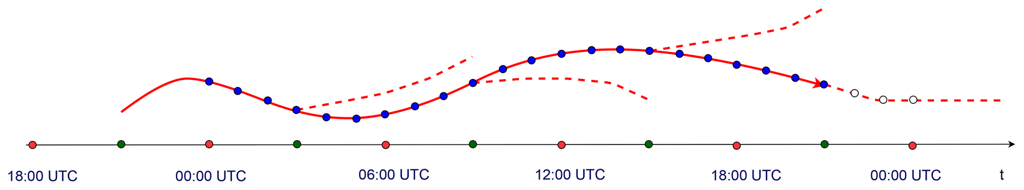
Figure 1Graphical representation of 4D-EnVar analysis cycle during 24 h using IAU initialization. The 4D-EnVar analyses are computed using a 6 h assimilation window centered at 00:00, 06:00, 12:00 and 18:00 UTC (red dots on the timescale). The GEM model (in coupled or uncoupled mode) 6 h integration using an IAU initialization of the analysis increments (solid lines) starts at 21:00, 03:00, 09:00 and 15:00 UTC (green dots on the timescale), followed by 6 h computation of the background states for the next analysis (dotted lines). The 21 blue dots show the atmospheric states, available hourly, used as atmospheric forcing at 1 h frequency for the NEMO–CICE model to compute coupled 24 h ocean background within WCDA (see text). The last three forcing states of every 24 h cycle are taken from the computation of the background fields (white dots).
The DA method is a hybrid four-dimensional ensemble-variational (4D-EnVar) (Buehner et al., 2013, 2015) using incremental analysis update (IAU) initialization (Bloom et al., 1996). The IAU implementation used with the GDPS system is illustrated in Fig. 1. The hybrid approach combines four-dimensional ensemble covariances with the static error covariances computed with so-called National Meteorological Center (NMC) method (Parrish and Derber, 1992) to estimate the full spatio-temporal background error covariances over the 6 h assimilation time window. The ensemble and static covariances are averaged with equal weights in the resulting full background error covariances. The ensemble covariances are estimated from the ensemble of 256 uncoupled background states, available hourly within the 6 h assimilation window, obtained from the global ensemble Kalman filter (EnKF) being used operationally at ECCC (Houtekamer et al., 2014) since 2005. The EnKF version used in this study (4.1.1) is the one that was operational at the time of the experiments. This version was replaced by an updated version in September 2018. The 4D-EnVar analysis increments are computed on a grid with a horizontal grid spacing of 50 km, as in the EnKF system, on all 80 vertical levels.
In the current version of the GDPS, the operationally assimilated data consist of those from microwave and infrared satellite sounders and imagers, scatterometers, radiosondes, aircrafts, wind profilers, land stations, near-surface observations from ships and buoys, atmospheric motion vectors, ground-based GPS sensors, and satellite-based radio occultation instruments. More details about the assimilated data may be found in Buehner et al. (2015).
The GEM model has been designed to be coupled with a land surface model; it is called ISBA: the Interactions between Soil–Biosphere–Atmosphere scheme (Noilhan and Planton, 1989). ISBA computes the surface heat and momentum fluxes over four surface types: land, glacier, water and sea ice. The prognostic surface variables of the current surface model are computed for the land surface only, which has its own DA system (Bélair et al., 2003). The land surface model and DA in both uncoupled and coupled DA experiments of this study are similar to what is currently used operationally. The definition of water and sea ice surfaces requires information from the external SST and sea ice DA components, as described in Sect. 2.3 and 2.4, respectively.
2.2 Ocean data assimilation
The ocean DA component used in this study is the same as the current operational Global Ice–Ocean Prediction System (GIOPS: Smith et al., 2016). The numerical model used is the NEMO–CICE coupled ocean–ice model based on NEMO (Nucleus for European Modelling of the Ocean) version 3.1.3 (Madec, 2008; Smith et al., 2018) and CICE (Community Ice CodE) version 4.0 (Hunke and Dukowicz, 1997; Hunke et al., 2010). The NEMO version used here has a global horizontal ORCA grid and 50 vertical levels ranging from the ocean surface to the ocean bottom with spacing increasing from 1 m at the surface to 500 m near the bottom. The thermodynamic component of CICE computes the growth and melt of snow and ice as well as the vertical temperature profile using four ice layers and one snow layer. The ocean upper boundary conditions are the turbulent surface latent, sensible, incoming and outgoing longwave and shortwave radiation fluxes.
The ocean DA system used is the Système d'Assimilation Mercator version 2 (SAM2) (Lellouche et al., 2013). The SAM2 DA algorithm is the singular evolutive extended Kalman (SEEK) filter derived from the Kalman filter (Pham et al., 1998). The background error covariances are estimated using an ensemble of multivariate three-dimensional anomalies derived from a multiyear hindcast simulation (Lellouche et al., 2013). The version used in this study is GIOPS v2.2.3, corresponding to the currently operational system.
The SAM2 DA consists of two successive DA cycles. First, in a weekly cycle, in situ data, SST and satellite altimetry data are assimilated. The in situ data are derived from multiple sources including the Argo floats (Gould, 2005), as well as ships, moorings and instrumentation on sea mammals. The satellite altimetry data are obtained from a product combining anomalies of the sea level with a mean dynamic topography. The sea level anomalies are provided by Archiving, Validation and Interpretation of Satellite Oceanographic data (AVISO), SSALTO/DUACS near-real-time data including Jason-2, and CryoSat-2 and SARAL/AltiKa satellite data. The CNES-CLS09 mean dynamic topography used is from Rio et al. (2011).
Second, in a daily assimilation cycle, only SST data are assimilated. The assimilated SST is itself a gridded analysis computed within the operational SST DA based on optimal interpolation (OI) as described in Sect. 2.3. It is designed to reduce initialization shocks for coupled forecasts by imposing consistent surface conditions on the atmosphere and ocean during their separate assimilation cycles. The assimilation of an SST OI analysis by an ocean analysis system is also fairly commonplace within the operational oceanographic community (e.g. by the Global Ocean Forecasting system within the Copernicus Marine Environmental Monitoring System; Lellouche et al., 2013). This approach has the benefit that it provides a pretreatment (or superobbing) of high-resolution SST observations, allowing for the assimilation of more satellite SST datasets. Since the coverage of satellite SST data is quite complete, data gaps do not produce a significant problem compared to the advantages of this approach. Within this second DA cycle, the sea ice analysis produced by the system described in Sect. 2.4 is also used to reinitialize the model ice concentration each day.
2.3 Sea surface temperature data assimilation
The SST DA system is described in detail in Brasnett (2008) and Brasnett and Colan (2016). The version used in this study is the operational SSTv1.2.2, which is currently employed in the operational implementation of the atmospheric GDPS system (see Sect. 2.1). The DA approach used in the system is the OI method producing daily analyses considered to be valid at 00:00 UTC. The assimilated data are collected during the period of 24 h before this valid time. The SST OI assimilates data from multiple in situ platforms (drifting and moored buoys, ships) and Advanced Very High Resolution Radiometer data provided by the US Naval Oceanographic Office that are derived following the multichannel SST (MCSST) approach (May et al., 1998; McClain et al., 1985). The SST DA system does not employ a numerical forecast model. Instead, it uses the previous analysis state computed 24 h earlier as the background state for the assimilation.
The assimilation of the SST data from multiple satellite instruments along with the in situ data is discussed in detail in Donlon et al. (2007). An important aspect of the system is the estimation and removal of observation biases. Indeed, the infrared radiometer measures the temperature within the conductive diffusion layer at a depth of ∼10–20 µm, or the so-called skin temperature. The microwave radiometer retrieves the sub-skin temperature at the base of the laminar layer at around 1 mm of depth. All these data need to be reconciled with the in situ temperature usually measured at a depth of ∼2 m. On the other hand, the current weather prediction system requires an SST field to be kept fixed through 24 h. To this end, the SST at a depth at which the effect of the diurnal cycle is negligible was required. Since the in situ observations are located sufficiently deep, the data from different satellite instruments are adjusted to the in situ data first. Second, a so-called foundation SST, the temperature at a depth without a diurnal cycle, is estimated. The estimation is performed in two stages. First, the background state, which is the anomaly field of the foundation SST, is computed by subtracting from the analysis of a previous state a precomputed monthly mean climatology interpolated in time. After the analysis state of the foundation SST anomaly has been computed, the climatological field interpolated to the current day is added to it to obtain the SST analysis state. The output of this system is a daily analysis of the foundation SST field on an uniform latitude–longitude grid. This field is used within both the GDPS (Sect. 2.1) and GIOPS (Sect. 2.2) DA components.
2.4 Sea ice data assimilation
The sea ice concentration DA system is based on the 3D-Var DA method (Buehner et al., 2016) implemented on a global domain at ∼10 km resolution. As for the atmospheric DA component described in Sect. 2.1, the sea ice analyses are computed every 6 h at 00:00, 06:00, 12:00 and 18:00 UTC. Similar to the SST analysis, the sea ice analysis system was originally developed using various sources of satellite data that generally have good combined spatial coverage globally every 6 h. This system was developed before our center became active in using sea ice models, and therefore it was for practical reasons that it does not use a model within the assimilation cycle but instead uses the previous analysis produced 6 h earlier as the background state for the assimilation. The 3D-Var sea ice analysis assimilates passive microwave satellite observations from the Special Sensor Microwave Imager (SSM/I), the Special Sensor Microwave Imager/Sounder (SSMIS) and the Canadian Ice Service (CIS) manual analyses (Carrieres et al., 1996; Buehner et al., 2016). Details about how these datasets were treated within the 3D-Var DA may be found in Buehner et al. (2016). The sea ice concentration analyses are used to initialize the atmospheric (see Sect. 2.1) and the ice–ocean (Sect. 2.2) forecast models to compute the background states for both uncoupled and coupled DA systems described in Sect. 3.
2.5 Coupled weather forecast model
In this section, the model used to produce medium-range forecasts in both the uncoupled and WCDA systems (see Sect. 3.1 and 3.2, respectively) is described. The system used in this study is the fully coupled atmosphere–ocean–ice GEM–NEMO–CICE model that was operationally implemented at ECCC for global NWP in November 2017 (Smith et al., 2018). This system is used to produce 10 d coupled atmosphere–ocean–ice forecasts initiated at 00:00 and 12:00 UTC. The atmospheric GEM model initial conditions are the corresponding 00:00 and 12:00 UTC atmospheric analyses (see Sect. 2.1) using the IAU initialization. The GEM model version used in this study is similar to the model described in Sect. 2.1 except for the modified ocean interface whereby the contributions from the ice–ocean model are transferred to the atmospheric model every model time step.
The coupled NEMO version is 3.1.3 and CICE is 4.0 as described in Sect. 2.2. However, the models are launched in a coupled mode that consists of a flux coupling approach described in detail in Roy et al. (2015) and Smith et al. (2018). This approach aims to simulate the interactive and consistent transfer of heat, moisture and momentum between the atmospheric and ocean–ice models. It is based on common atmospheric, oceanic and sea ice state variables. First, the atmospheric model computes downward radiative fluxes and state variables and then transfers this information to the ocean–ice model. Second, these fluxes and variables are used by the ocean model to compute turbulent upward surface atmospheric fluxes using the same formulation as used within the atmospheric GEM model (Delage and Girard, 1992; Delage, 1997). The turbulent surface fluxes over the ice-covered areas are computed within the CICE model using stability functions described in Jordan et al. (1999). Finally, the surface fluxes are transferred to the atmospheric model along with the SST and sea ice at every model time step of 15 min. The time stepping of the coupled atmosphere–ocean–ice model is implemented such that the atmospheric model moves forward one step ahead of the ocean–ice model prior to sending its variables.
The initial conditions for the NEMO ocean model are obtained from the daily SAM2 analyses at 00:00 UTC (Sect. 2, 2.2) for both forecasts launched at 00:00 and 12:00 UTC. The 00:00 and 12:00 UTC initial conditions for the CICE ice model are obtained from the 3D-Var DA (Sect. 2.4) computed at 18:00 UTC of the previous day, which normally assimilates more data than the analyses computed at 00:00, 06:00 and 12:00 UTC.
In the present section, the uncoupled DA (referred to as UNCPL) and WCDA (referred to as CPL) configurations of the complete forecast–analysis cycles are discussed. UNCPL is similar to the combined set of uncoupled systems currently used at ECCC for the operational production of forecasts. This system will be used in this study as a reference to evaluate the performance of the new CPL system. Both systems use the DA and model components described in Sect. 2. The differences in design between UNCPL and CPL are in the assimilation cycles, whereas initial conditions from both UNCPL and CPL are used to initialize fully coupled atmosphere–ocean–ice 10 d forecasts (Sect. 2.5).
3.1 Uncoupled data assimilation
The graphical scheme of the uncoupled DA cycle is shown in Fig. 2. The atmospheric 4D-EnVar (Sect. 2.1) analyses are computed four times per day at 00:00, 06:00, 12:00 and 18:00 UTC. The uncoupled atmospheric GEM model is initialized using IAU during 6 h integration centered at the analysis time, followed by the 6 h GEM model integration to compute the background state for the next atmospheric DA (see Fig. 1). The GEM model forecast is computed using the SST and sea ice fields specified by the separate DA systems described in Sect. 2.3 and 2.4, respectively. The GEM model version used in this system is the same as described in Sect. 2.1.
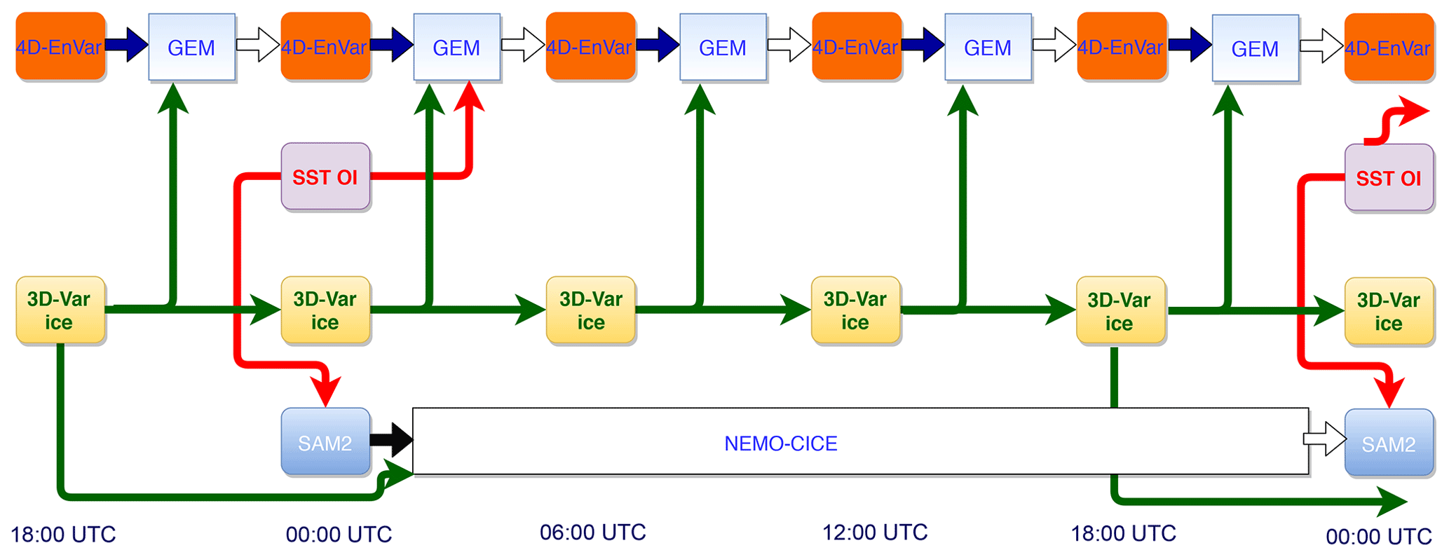
Figure 2The uncoupled DA system (UNCPL) scheme. The atmospheric 4D-EnVar DA component computes analyses every 6 h. The SST OI DA component computes daily analyses valid at 00:00 UTC, which initialize the atmospheric GEM model and are assimilated using the daily SAM2 ocean DA component at 00:00 UTC. The 3D-Var ice analyses are computed every 6 h and are used to initialize the uncoupled 6 h atmospheric and 24 h oceanic uncoupled forecasts. The uncoupled atmospheric analyses are propagated in space and time using the GEM model. The uncoupled ocean analyses are propagated using the NEMO–CICE model.
The weekly SAM2 ocean DA system for in situ data and satellite altimetry is used in the same way in both UNCPL and CPL systems and is not shown. The daily ocean SAM2 DA (Sect. 2.2), assimilating only SST daily mean data, is computed at 00:00 UTC. The ocean–ice NEMO–CICE model is initialized using IAU during a 24 h model integration starting 24 h before the current analysis time, followed by another 24 h NEMO–CICE model integration (see Sect. 2.2) to compute the background state for the next daily ocean DA. The ocean–ice NEMO–CICE model forecast during 24 h is run in uncoupled mode using the atmospheric forcing fields from the GEM model forecast at 3 h frequency started at 00:00 UTC.
The 3D-Var sea ice DA (Sect. 2.4) computes analyses every 6 h, providing the ice concentration field used for the short-term forecasts used to produce the atmospheric background state. The 3D-Var sea ice analysis computed at 18:00 UTC is used for initializing the 24 h ocean–ice forecast used as the background state for the following day. The SST OI analysis (Sect. 2.3) computed at 00:00 UTC provides the static SST field used for the following four 6 h atmospheric forecasts used as the background states during 24 h. The same SST analysis is also assimilated into the SAM2 daily ocean DA system (see Sect. 2.2).
3.2 Weakly coupled data assimilation
The graphical scheme of the CPL cycle, combining coupled 6 h atmospheric and 24 h ocean DA systems, is shown in Fig. 3. The atmospheric 4D-EnVar analyses (Sect. 2.1) are computed every 6 h (see Fig. 1) exactly as in the UNCPL system described in the previous section. However, the fully coupled atmosphere–ocean–ice model (see Sect. 2.5) is used within CPL to compute the coupled atmospheric background states for the atmospheric DA.

Figure 3WCDA system (CPL) scheme. The atmospheric 4D-EnVar DA component computes analyses every 6 h. The SST OI DA component computes daily analyses valid at 00:00 UTC, which are assimilated using the daily SAM2 ocean DA component at 00:00 UTC. The 3D-Var sea ice analyses are computed every 6 h. The 3D-Var sea ice analysis computed at 18:00 UTC provides the initial condition for the computation of fully coupled atmosphere–ocean background states at 00:00, 06:00, 12:00 and 18:00 UTC. The separate atmospheric and ocean analyses are propagated in space and time using the fully coupled GEM–NEMO–CICE model.
Only the atmospheric DA component of the CPL system explicitly uses the fully coupled atmospheric–ocean–ice model to compute the background states. To compute the observation-minus-background difference, the SAM2 ocean DA component directly uses the ocean–ice model launched in a forced mode, i.e. using precomputed atmospheric forcing fields. However, by saving the atmospheric fields from the 6 h coupled forecasts and using these to force the ocean model, this is equivalent to the explicit use of the fully coupled atmosphere–ocean–ice model. Using the precomputed atmospheric forcing fields from the coupled ocean–atmosphere forecasts allows us to implicitly compute coupled ocean background states without modifying the SAM2 code. Preliminary experiments showed that the use of the precomputed atmospheric forcing from the fully coupled model every hour gives results similar to the forcing changing every model time step (the ocean–ice model time step is 15 min in our experiments). So the frequency of the atmospheric forcing has been set to 1 h.
Hence, in order to compute coupled 24 h background states for the ocean DA, the CPL system first performs four atmospheric 6 h DA cycles as shown in Fig. 1. The coupled atmospheric states from the coupled atmosphere–ocean–ice model integrations during the application of IAU are stored every 1 h during this stage. To cover the whole 24 h cycle, the last three states are taken from the coupled background fields because the states during the use of IAU at 22:00, 23:00 and 00:00 UTC are not yet available in the current 24 h DA cycle.
Once the entire 24 h period of atmospheric forcing (following the approach just described) is available, the ocean DA starts by integrating the ocean–ice model over the 24 h period to compute the observation-minus-background differences for SST. From these differences, the daily SAM2 ocean DA then computes analysis increments. The ocean analysis increment is then used to rerun the ocean–ice model over the same 24 h period using the same atmospheric forcing. This provides the initial conditions for the next 24 h cycle.
As in UNCPL, the 3D-Var sea ice analysis (Sect. 2.4) is computed every 6 h. However, only the analysis at 18:00 UTC is used to initialize the computation of four 6 h fully coupled atmosphere–ocean forecasts used as background states during 24 h exactly as it is implemented in the coupled weather forecast model (see Sect. 2.5). The SST OI analysis (Sect. 2.3) is computed at 00:00 UTC and assimilated by the daily ocean SAM2 DA component as in the UNCPL system.
The experiments are conducted for the period of August–September 2017. The verification statistics shown in this section are computed between 15 August and 20 September during which a series of tropical Atlantic hurricanes occurred. Two 5 d forecasts per day at 00:00 and 12:00 UTC are carried out over this period. The atmospheric and ocean–ice initial conditions for all experiments are taken from the DA systems described in Sect. 3.1 and 3.2. The comparison study focuses on the differences in the atmospheric and ocean forecasts and the analyses produced by the CPL and UNCPL systems. Differences between these two systems are expected for the forecasts of SST and near-surface layers in both atmosphere and ocean models.
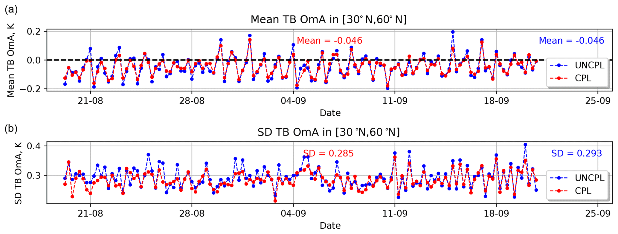
Figure 4(a) Observation-minus-analysis (OmA) statistics: mean (a) and standard deviation (b) using 6 h forecasts. Mean and standard deviation for the brightness temperature (K) as seen by the AQUA AIRS channel 950. The statistics are computed for UNCPL (blue) and CPL (red) in the northern extratropics region between 30 and 60∘ N.
The use of a coupled model between the atmosphere and the ocean–ice to compute the background state may lead to changes in both atmosphere and ocean DA. Concerning the atmosphere, these changes may be seen, for example, using satellite radiances that are sensitive to the temperature of the ocean. Such instruments measure radiance within the atmospheric window; i.e. the sensitivity to the atmospheric temperature and humidity is low, which allows the emission from the ocean surface temperature to be measured. In order to illustrate the impact of the evolving ocean surface temperature on the atmospheric DA, the evolution of the observation-minus-analysis (OmA) and the observation-minus-forecast (OmF) biases as well as the standard deviation are computed for the brightness temperature (TB) of the AQUA AIRS channel 950 (see Figs. 4 and 5, respectively). 6 h forecasts are used to compute the OmF biases and standard deviation. Generally, both OmA and OmF biases for this atmospheric window channel for UNCPL and CPL are similar. However, the CPL experiment results in smaller OmA and OmF standard deviations than UNCPL. Overall relative to UNCPL, the CPL standard deviations are reduced by 2.7 % for OmA and 1.9 % for OmF. For the OmA and OmF biases, we clearly see a 24 h period, so it is likely related to the diurnal cycle. However, for the standard deviation, it looks like a 12 h variation, so it is not due to the diurnal cycle. This effect is probably related to the data coverage.

Figure 5Observation-minus-forecast (OmF) statistics: mean (a) and standard deviation (b) using 6 h forecasts. Mean and standard deviation for the brightness temperature (K) as seen by the AQUA AIRS channel 950. The statistics are computed for UNCPL (blue) and CPL (red) in the northern extratropics region between 30 and 60∘ N.
Such improvements in the OmF–OmA statistics for atmospheric window channel radiances may also be reflected in improvements of the medium-range atmospheric forecast. Figure 6 shows the difference in the standard deviation of the forecasted atmospheric temperature against the mean analysis (mean between the two experiments: CPL and UNCPL) for different pressure levels between 1000 and 10 hPa as a function of the forecast lead time. Red shows the lead times and pressure levels at which CPL performs better (i.e. has a lower standard deviation) than UNCPL, and blue shows the converse. The score shown in the figure is computed in the northern extratropics region in the latitude band between 20 and 60∘ N. In most cases, CPL performs slightly better than UNCPL. A statistically significant difference with confidence above 90 % is only observed for the near-surface air temperature at around 1000 hPa for the 12 and 36 h forecasts (the difference is statistically insignificant elsewhere). Similar forecast scores computed for the geopotential height and specific humidity also show slightly better performance for CPL but with no areas in which the improvement is statistically significant (not shown). The impact of CDA on forecast scores computed for the wind field is rather neutral (not shown). Similar results were also obtained when the ERA5 reanalysis is used instead of the mean analysis (also not shown).
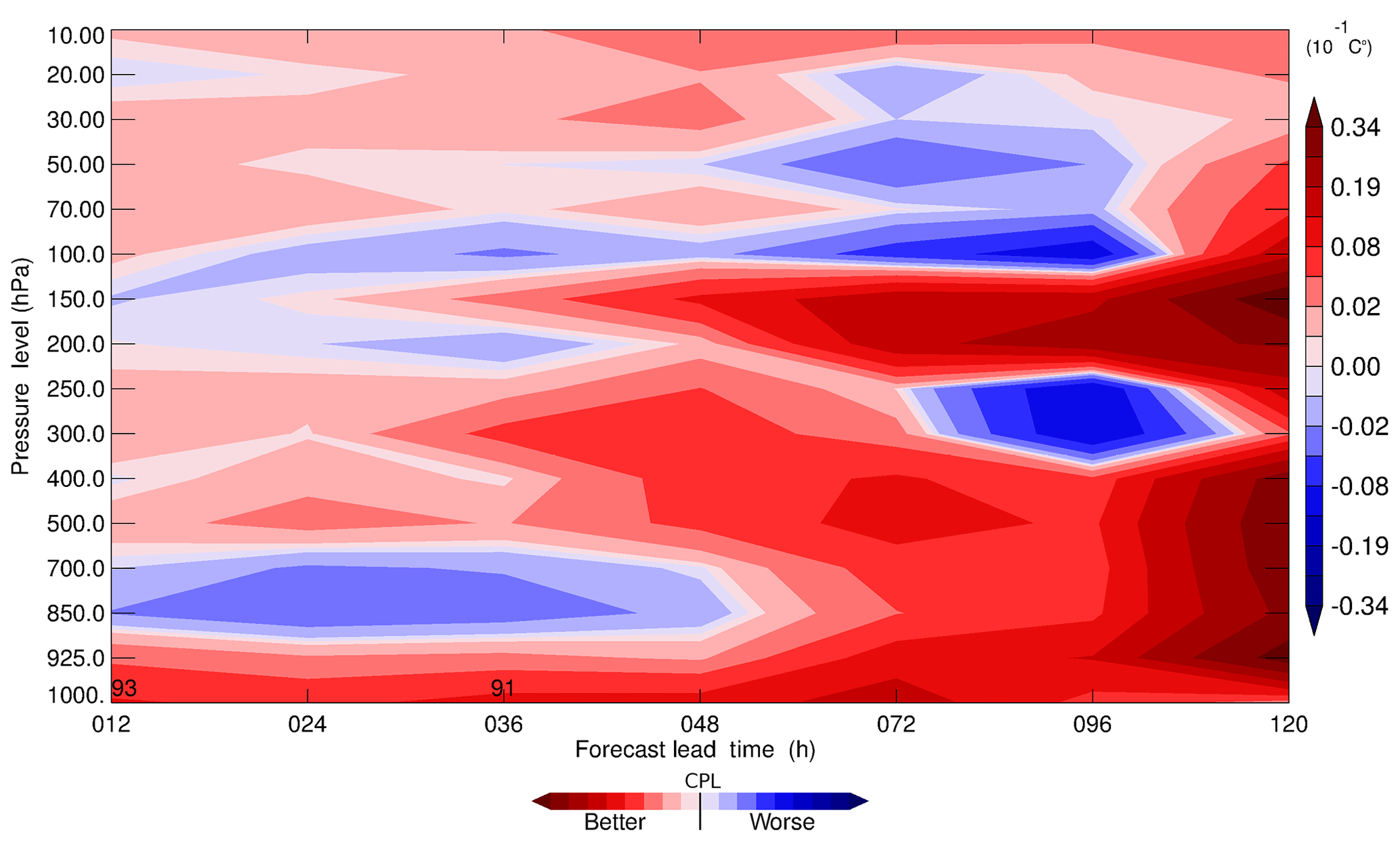
Figure 6Difference in the standard deviation of the air temperature (∘C) against the mean analysis as a function of forecast lead time. The statistics are computed for CPL and UNCPL in the northern extratropics region between 20 and 60∘ N. Positive values (red) mean that the standard deviation produced by CPL is smaller, whereas negative values (blue) mean the converse. Numbers show the areas where the difference between CPL and UNCPL is statistically significant with a confidence level above 90 %.
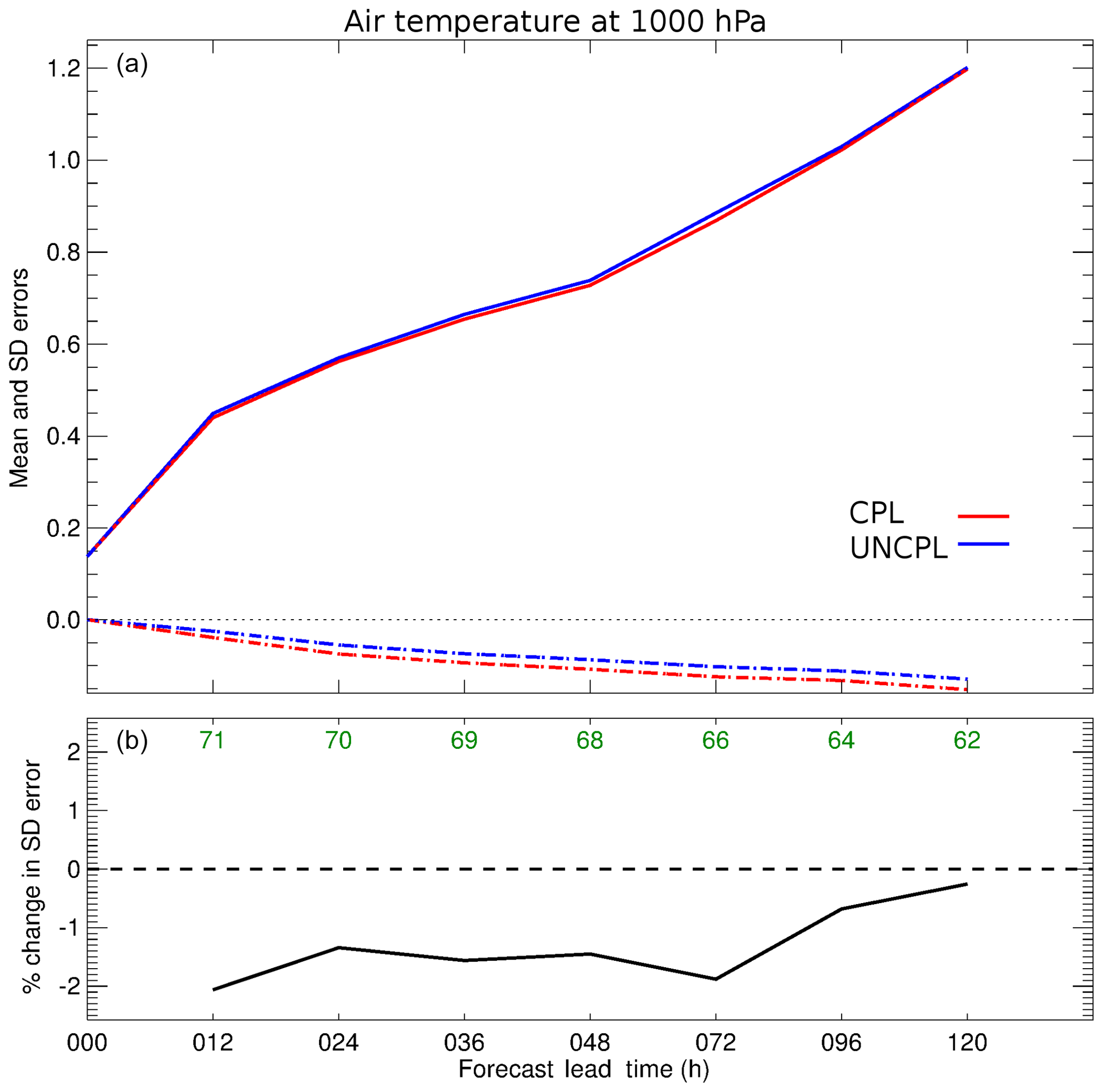
Figure 7(a) Standard deviation (solid curves) and bias (dashed curves) growth (∘C) as a function of forecast lead time for the air temperature at 1000 hPa. The statistics are computed for the CPL (red) and UNCPL (blue) against the mean analysis in the northern extratropics region between 20 and 60∘ N. (b) The difference in the standard deviation error in percent between CPL and UNCPL. Green indicates the number of samples used to compute the statistics.
Figure 7 helps to highlight the better performance of CPL for the forecast of near-surface air temperature over the same northern extratropics region. Figure 7a shows the standard deviation and bias of the air temperature at 1000 hPa against the mean analysis as a function of the forecast lead time. Figure 7b shows the difference between the standard deviations of the CPL and UNCPL. The CPL experiment results in a standard deviation which is about 2 % smaller than the corresponding value from the UNCPL experiment. However, CPL results in a larger negative bias in the same area.
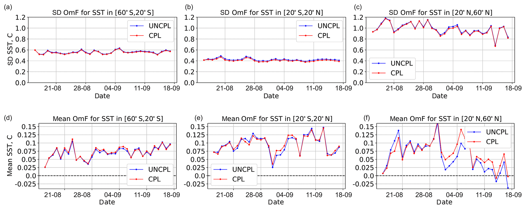
Figure 8Evolution of sea surface temperature OmF standard deviation (a, b, c) and mean OmF (d, e, f) (∘C) with respect to SST data assimilated within the separate SST DA component. The statistics are computed for UNCPL (blue curves) and CPL (red curves) in three latitude bands: southern extratropics between 20 and 60∘ S (a, d), tropics, between 20 and 20∘ N (b, e), and northern extratropics between 20 and 60∘ N (c, f). The statistics are computed for the 12 h forecast and the corresponding data.
Let us now examine the quality of SST forecasts from the CPL and UNCPL experiments. Figure 8 shows the evolution of OmF standard deviation and mean OmF for SST computed with respect to the original satellite and in situ observations that were used within the SST DA system described in Sect. 2.3. The OmF statistics are computed for the 12 h coupled forecasts produced using the CPL and UNCPL initial conditions in three different latitude bands: southern extratropics between 20 and 60∘ S, tropics between 20∘ S and 20∘ N, and northern extratropics between 20 and 60∘ N. The OmF standard deviations produced by CPL are systematically lower than those produced by UNCPL in all three regions, whereas the mean OmF produced by CPL is sometimes larger. The differences for the mean OmF are small and also not systematically in favor of one experiment over the other (as opposed to the difference for the standard deviation of OmF). Due to this variation in the differences for the mean OmF and the relatively short length of the experiments, we are not confident in the statistical significance of the differences.
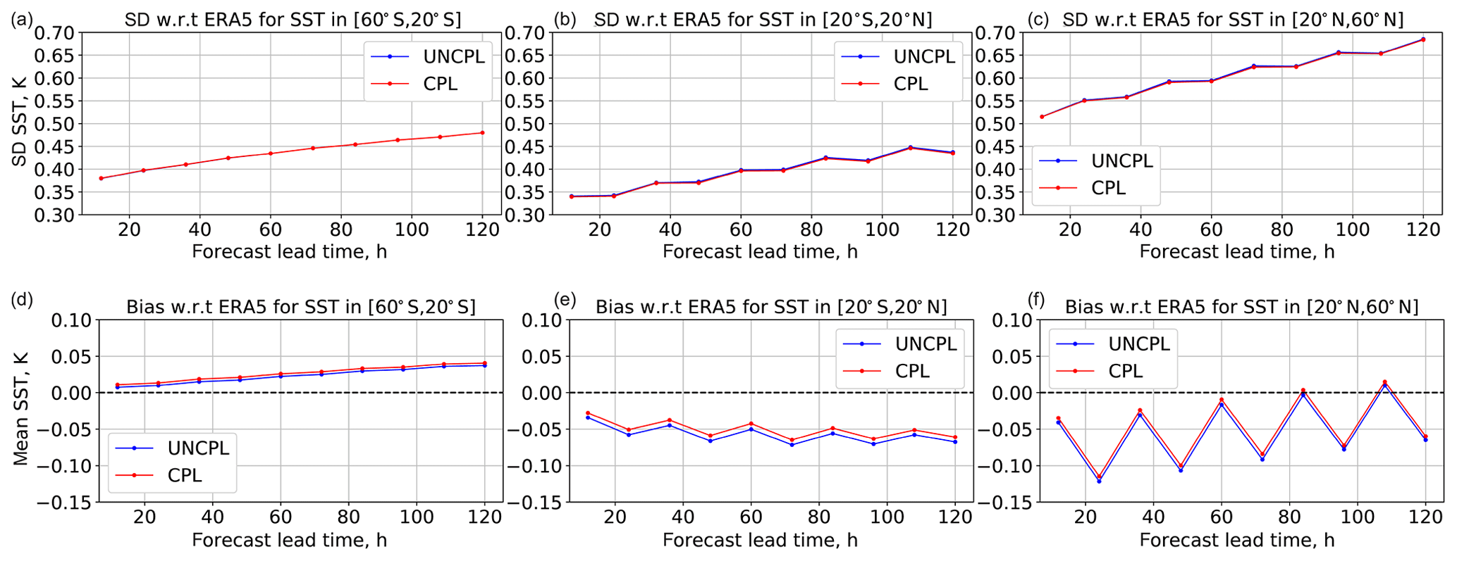
Figure 9Standard deviation (a, b, c) and bias (d, e, f) (K) with respect to the ERA5 reanalysis daily mean SST fields as a function of forecast lead time. The statistics are computed for UNCPL (blue curves) and CPL (red curves) in three latitude bands: southern extratropics between 20 and 60∘ S (a, d), tropics between 20∘ S and 20∘ N (b, e), and northern extratropics between 20 and 60∘ N (c, f).
Figure 9 shows the SST standard deviation and bias from the coupled medium-range forecasts produced using the CPL and UNCPL initial conditions in the same three latitude bands as in the previous figure. The standard deviation and bias are computed as a function of the forecast lead time with respect to the daily mean OSTIA product (Donlon et al., 2012) used in the ECMWF ERA5 reanalysis generated using Copernicus Climate Change Service information. This product was chosen to evaluate the forecasts from our experiments because it can be considered an independent dataset. Another high-quality SST product, the Group for High Resolution SST (GHRSST) Multi-Product Ensemble (GMPE) system (Martin et al., 2012), was not chosen because it partially uses the same SST analyses from ECCC as described in Sect. 2.3. The standard deviations are similar for both experiments in all three latitude bands, with slightly smaller values in the tropics for CPL. The bias produced by CPL is smaller in the tropics and northern extratropics and slightly bigger in the southern extratropics. The coupled forecasts represent the diurnal cycle to some extent for the SST, which is not captured in the ERA5 SST analyses (since it is a foundation SST). Therefore, for the northern extratropics the mean difference in SST has a strong daily cycle since the Pacific Ocean dominates the oceanic surface area at these latitudes, which is mostly day at 00:00 and night at 12:00 UTC. In contrast, the other regions have more even oceanic coverage at all longitudes (especially for the southern extratropics) and therefore have a more even coverage of day and night at both 00:00 and 12:00 UTC.

Figure 10OmF standard deviation (a) and mean (b) with respect to the gridded foundation SST field from the ocean SAM2 DA component for the Puerto Rico XBT region situated within the latitude–longitude box defined by [35, 65∘ W] and [25, 35∘ N]. The statistics are computed using 24 h forecasts.
Similar error statistics for SST can be computed within the ocean DA system described in Sect. 2.2. Figures 10 and 11 compare the SST OmF standard deviation and bias computed using 24 h forecasts within the CPL and UNCPL experiments. The error statistics are computed relative to the gridded foundation SST field obtained from the SST DA that was assimilated by the daily SAM2 ocean DA as explained in Sect. 2.2. The use of the analysis field to compute the standard deviation and biases affects the spatial sampling compared to OmF statistics against the SST satellite and in situ data shown in Fig. 8. The figures show two typical OmF plots computed in the Puerto Rico XBT region, showing the performance in the western tropical and northern extratropical Atlantic Ocean, and the Niño3 region in the tropical Pacific Ocean. The CPL results in generally smaller OmF biases and standard deviation errors in most regions.
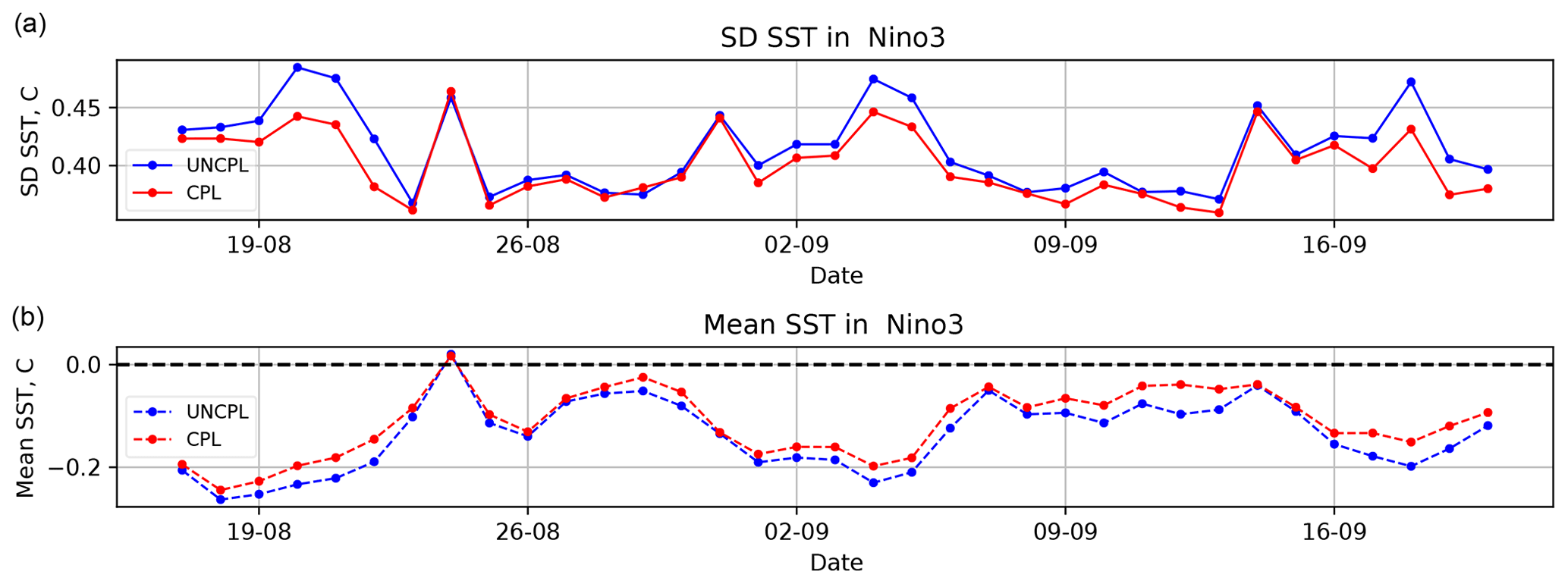
Figure 11OmF standard deviation (a) and mean (b) with respect to the gridded foundation SST field from the ocean SAM2 DA component for the Niño3 region situated within the latitude–longitude box defined by [150, 90∘ W] and [5∘ S, 5∘ N]. The statistics are computed using 24 h forecasts.
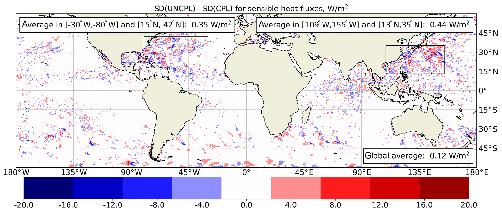
Figure 12Difference (W m−2) between the standard deviation of UNCPL and CPL for the turbulent surface sensible heat flux computed using 12 h coupled forecasts during September 2017.
The changes in the SST may modify the turbulent surface heat flux forecasts. To qualitatively evaluate the impact of CDA on the fluxes, the standard deviations for the turbulent surface sensible heat flux were computed using short 12 h coupled forecasts produced with the UNCPL and CPL initial conditions during September 2017. Figure 12 shows the difference between the two standard deviation fields. Positive values (red) mean that the standard deviation of the flux from the UNCPL experiment is bigger than the standard deviation from the CPL experiment, whereas negative values (blue) mean the converse. The decrease in the standard deviations of the surface sensible heat flux reflects a better accordance between the near-surface atmospheric temperature and the SST. While the same gridded SST OI analysis is assimilated in the ocean and used for the surface boundary condition in UNCPL, differences remain between the SST of the ocean analysis and the OI analysis. The OI analysis is assimilated with a 0.3 ∘C observation error by the ocean analysis, and thus differences of up to 1.0 ∘C can be found. These differences are especially apparent in energetically active areas of the ocean (due to small-scale eddies not captured in the OI analysis) as well as due to the presence of cyclones (e.g. due to cold wakes). As a result, surface fluxes in UNCPL forecasts will reflect this imbalance in initial conditions. In most regions, the impact of CDA on the surface sensible heat flux is neutral except the northern extratropical Atlantic, where a series of tropical Atlantic hurricanes occurred, as well as in the northern extratropical Pacific. In these regions, positive differences of 8–16 W m−2 and negative differences of 4–8 W m−2 are observed, though the number of positive differences is bigger. Similar spatial structures but with smaller values are observed when the same quantities are computed for the surface latent heat flux (not shown). It was noted during the evaluation of the fully coupled atmosphere–ocean–ice model (Smith et al., 2018) that interactions on the surface interface resulted in a reduced latent heat flux due to the formation of cold wakes associated with cyclones, leading to reduced intensification. Inclusion of the fully coupled atmosphere–ocean–ice model in the computation of background states improves the representation of these interactions in the analysis, resulting in a further decrease in the variance of fluxes (i.e. likely due to the reduced intensification of cyclones).

Figure 13Difference between the UNCPL and CPL (24 h forecasts) RMSE (∘C) with respect to the Argo ocean temperature measurements in September 2017. Positive values (red) indicate that the RMSE produced by CPL is smaller, whereas negative values (blue) mean the converse. (a) The RMSE difference for ocean temperature at 2.5 m of depth. The grey areas show the regions where Argo measurements were not taken. (b) The temperature vertical section through 1.5∘ N latitude in the eastern tropical Pacific Ocean between 120 and 100∘ W.
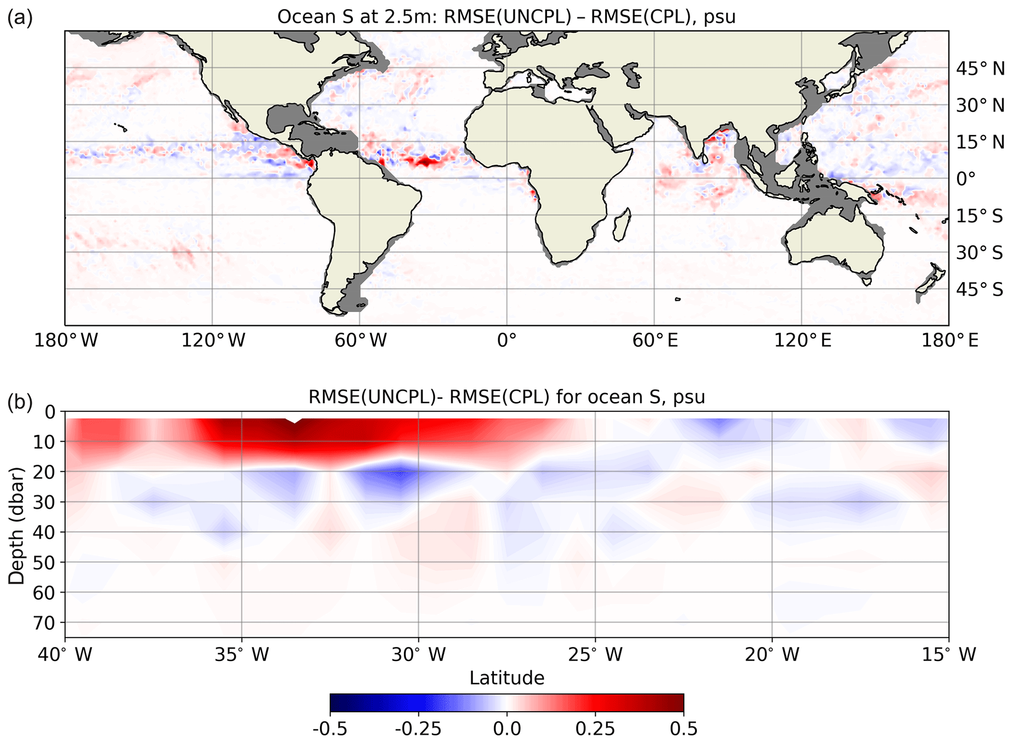
Figure 14Difference between the UNCPL and CPL (24 h forecasts) RMSE (psu) with respect to the Argo ocean salinity measurements in September 2017. Positive values (red) indicate that the RMSE produced by CPL is smaller, whereas negative values (blue) mean the converse. (a) The RMSE difference for ocean salinity at 2.5 m of depth. The grey areas show the regions where Argo measurements were not taken. (a) The salinity vertical section through 6.5∘ N latitude in the tropical Atlantic Ocean between 40 and 15∘ W.
Finally, let us examine the impact of the WCDA on the subsurface ocean circulation. Figures 13 and 14 show the difference between the root mean square error (RMSE) for the monthly mean 24 h forecasts produced using UNCPL and CPL initial conditions relative to the Argo ocean temperature and salinity, respectively. The data used for the comparison are gridded fields using a global horizontal grid and 58 vertical levels obtained from the “Monthly mean datasets of the mean and annual cycle of temperature, salinity, and steric height in the global ocean from the Argo Program” (Roemmich and Gilson, 2009) downloaded from http://sio-argo.ucsd.edu/RG_Climatology.html (last access: 23 January 2019). Positive values (red) indicate that the RMSE of CPL is smaller, whereas negative values (blue) mean the converse. Figures 13a and 14a show the RMSE differences for ocean temperature and salinity at 2.5 m of depth, respectively. Figures 13b and 14b show vertical sections of the differences between the RMSE from the UNCPL and CPL experiments. The vertical section for temperature is plotted through 1.5∘ N latitude between 120 and 100∘ W. In most areas, CPL results in smaller temperature errors than UNCPL. The biggest differences for ocean temperature between the UNCPL and CPL experiments are observed in the eastern tropical Pacific, where the biggest positive differences of about 0.45 ∘C form a front with the biggest negative values of about −0.5 ∘C. Also for the vertical section, the errors produced by CPL are generally smaller in most areas between the ocean surface and 80 m of depth. Below this depth, the difference between the CPL and UNCPL experiments is negligible. For ocean salinity (Fig. 14), both CPL and UNCPL result in a similar RMSE except in the tropics, where CPL produces a lower RMSE than UNCPL. The biggest values of the RMSE differences, around 0.55 psu, are observed in the tropical Atlantic, where the vertical section of the RMSE differences for ocean salinity is shown through 6.5∘ N latitude between 40 and 15∘ W (Fig. 14b). In this area CPL produces a lower RMSE for salinity between the surface and 20 m of depth. The differences in salinity between the UNCPL and CPL experiments are negligible below 70 m of depth.
A WCDA system between the atmosphere and ocean DA components is implemented and evaluated in this study. The first prototype of the WCDA is built on the existing components of the NWP and operational ocean–ice prediction systems that have been previously run as independent uncoupled DA systems. As the NWP system requires SST and ice concentration fields and the quality of ocean–ice prediction depends on atmospheric forcing, the transition from uncoupled to strongly coupled DA should be smooth and gradual in order to not degrade the quality of the existing atmospheric and ocean–ice prediction systems.
The first step towards CDA was to replace the uncoupled models used to compute the background state for each DA with the fully coupled atmosphere–ocean–ice model within separate atmosphere and ocean DA components. The ocean community model NEMO has already been coupled with atmospheric models to perform WCDA in multiple studies. However, the atmospheric GEM model and the 4D-EnVar DA were never tested before in a coupled framework. The present study showed that the use of the coupled atmosphere–ocean–ice model to compute the background states for separate atmospheric and ocean DA systems has a generally neutral to positive effect on the 5 d atmospheric forecasts. However, the verification scores from WCDA are significantly better up to day 4 in the near-surface atmospheric layers in the tropics and northern extratropics. WCDA also leads to better agreement between the near-surface atmospheric temperature and the SST, locally decreasing the variability of turbulent surface heat fluxes compared to uncoupled DA. Such encouraging results are obtained using the same configuration of the fully coupled atmosphere–ocean–ice model that was used operationally within the NWP system with no additional tuning of the model and allows one to explore further aspects of stronger coupling.
The improvement in the OmF standard deviation error for the near-surface air temperature is accompanied by a slight increase in the bias for the same forecast lead times and pressure levels. It may be related to the current formulation of the error covariances that do not include cross-correlation terms between different DA components.
Another positive result is that the quality of ocean forecasts for SST and salinity with respect to both standard deviation errors and biases is improved when using the coupled background states for the ocean DA. This is noted by smaller verification errors for the ocean temperature and salinity, especially in the tropics. This result is obtained despite the fact that the ocean DA, as the atmospheric DA, does not employ the cross-correlation error covariances. Longer experiments are needed to further explore this issue. The test period of 2 months used here might also be too short to see major changes in the ocean component. Thus, the results presented here should be viewed in this context.
As for the different impacts of WCDA in experiments carried out by the ECMWF and Met Office, there could be multiple reasons for starting from the most obvious, such as differences in coupling strategies, models, data assimilation methods and assimilated observations. However, what is clearly different in our system with respect to others is the ocean data assimilation system that uses two DA cycles, one with a weekly assimilation time window and the other with a daily window. As stated in the paper, the weekly DA cycle is not affected by the coupling process and will therefore prevent the deep ocean state from diverging between the UNCPL and CPL systems. In fact, every 7 d, the ocean is restarted from the same uncoupled initial conditions in both the UNCPL and CPL systems. This certainly affects the results, especially in the ocean, keeping it relatively close to the uncoupled solution. The small positive impact of WCDA on the ocean forecast that we observe is likely attributed to the better consistency between the ocean and atmosphere when using the coupled analysis, which reduces the initial shocks in the coupled forecasts.
In the current design of this first WCDA prototype, the daily ocean DA is mainly constrained by uncoupled SST and ice concentration analyses that do not rely on numerical models to compute background states. This weakens the degree of coupling because the daily initial condition for the whole atmosphere–ocean–ice system remains close to the uncoupled trajectory, and a certain time is needed to synchronize such initial conditions with the coupled model trajectory. The next step towards a stronger coupling would be to modify the SST and sea ice concentration analyses such that they operate within a 6 h cycle and use coupled background states. The transition from a daily to the 6 h SST analysis will require a new bias correction scheme for the SST data in order to properly estimate the ocean temperature diurnal cycle. In addition, the purely technical step of using integrated software for the atmosphere, SST and sea ice analysis will be necessary as an initial step before exploring stronger coupling by introducing background error cross-covariances between atmosphere and ocean components. This system may also be extended to perform the analysis for the whole ocean mixed layer, not only SST, every 6 h. These 6 h analyses may replace the current daily ocean DA system. This is the general orientation of future work.
The codes, scripts and data used in this paper are available for the topical editor and anonymous reviewers.
SS, MB, SL and GS were responsible for the concept. SS contributed to writing and original draft preparation. MB, LG and SL contributed to writing, review and editing. SS, EL, FR, DS-C and J-MB were responsible for software.
The authors declare that they have no conflict of interest.
The authors would like to acknowledge Pierre Pellerin, Pierre Koclas, Nicolas Gasset, Jean-François Caron, Kristjan Onu, Mateusz Reszka, Kamel Chikar, Sylvain Heilliette, Charles Creese, Richard Ménard and many others for fruitful discussions and collaborative work on common software tools. The authors also wish to thank the topical editor, Sophie Valcke, and two anonymous referees for the constructive review.
This paper was edited by Sophie Valcke and reviewed by two anonymous referees.
Bauer, P. and Richardson, D.: New model cycle 40r1, ECMWF Newsletter, available at: https://www.ecmwf.int/node/14581 (last access: 30 September 2019), 2014. a
Bélair, S., Crevier, L.-P., Mailhot, J., Bilodeau, B., and Delage, Y.: Operational Implementation of the ISBA Land Surface Scheme in the Canadian Regional Weather Forecast Model. Part I: Warm Season Results, J. Hydrometeorol., 4, 352–370, https://doi.org/10.1175/1525-7541(2003)4<352:OIOTIL>2.0.CO;2, 2003. a, b
Bloom, S. C., Takacs, L. L., da Silva, A. M., and Ledvina, D.: Data Assimilation Using Incremental Analysis Updates, Mon. Weather Rev., 124, 1256–1271, https://doi.org/10.1175/1520-0493(1996)124<1256:DAUIAU>2.0.CO;2, 1996. a
Brasnett, B.: The impact of satellite retrievals in a global sea-surface-temperature analysis, Q. J. Roy. Meteor. Soc., 134, 1745–1760, https://doi.org/10.1002/qj.319, 2008. a
Brasnett, B. and Colan, D. S.: Assimilating Retrievals of Sea Surface Temperature from VIIRS and AMSR2, J. Atmos. Ocean. Tech., 33, 361–375, https://doi.org/10.1175/JTECH-D-15-0093.1, 2016. a
Brassington, G., Martin, M., Tolman, H., Akella, S., Balmeseda, M., Chambers, C., Chassignet, E., Cummings, J., Drillet, Y., Jansen, P., Laloyaux, P., Lea, D., Mehra, A., Mirouze, I., Ritchie, H., Samson, G., Sandery, P., Smith, G., Suarez, M., and Todling, R.: Progress and challenges in short- to medium-range coupled prediction, J. Oper. Oceanogr., 8, s239–s258, https://doi.org/10.1080/1755876X.2015.1049875, 2015. a
Browne, P. A., de Rosnay, P., Zuo, H., Bennett, A., and Dawson, A.: Weakly Coupled Ocean–Atmosphere Data Assimilation in the ECMWF NWP System, Remote Sensing, 11, https://doi.org/10.3390/rs11030234, 2019. a
Buehner, M., Morneau, J., and Charette, C.: Four-dimensional ensemble-variational data assimilation for global deterministic weather prediction, Nonlin. Processes Geophys., 20, 669–682, https://doi.org/10.5194/npg-20-669-2013, 2013. a
Buehner, M., McTaggart-Cowan, R., Beaulne, A., Charette, C., Garand, L., Heilliette, S., Lapalme, E., Laroche, S., Macpherson, S. R., Morneau, J., and Zadra, A.: Implementation of Deterministic Weather Forecasting Systems Based on Ensemble–Variational Data Assimilation at Environment Canada. Part I: The Global System, Mon. Weather Rev., 143, 2532–2559, https://doi.org/10.1175/MWR-D-14-00354.1, 2015. a, b, c
Buehner, M., Caya, A., Carrieres, T., and Pogson, L.: Assimilation of SSMIS and ASCAT data and the replacement of highly uncertain estimates in the Environment Canada Regional Ice Prediction System, Q. J. Roy. Meteor. Soc., 142, 562–573, https://doi.org/10.1002/qj.2408, 2016. a, b, c
Carrieres, T., Greenan, B., Prinsenberg, S., and Peterson, I.: Comparison of Canadian daily ice charts with surface observations off Newfoundland, winter 1992, Atmos.-Ocean, 34, 207–226, https://doi.org/10.1080/07055900.1996.9649563, 1996. a
Charron, M., Polavarapu, S., Buehner, M., Vaillancourt, P. A., Charette, C., Roch, M., Morneau, J., Garand, L., Aparicio, J. M., MacPherson, S., Pellerin, S., St-James, J., and Heilliette, S.: The Stratospheric Extension of the Canadian Global Deterministic Medium-Range Weather Forecasting System and Its Impact on Tropospheric Forecasts, Mon. Weather Rev., 140, 1924–1944, https://doi.org/10.1175/MWR-D-11-00097.1, 2012. a
Côté, J., Desmarais, J.-G., Gravel, S., Méthot, A., Patoine, A., Roch, M., and Staniforth, A.: The Operational CMC–MRB Global Environmental Multiscale (GEM) Model. Part II: Results, Mon. Weather Rev., 126, 1397–1418, https://doi.org/10.1175/1520-0493(1998)126<1397:TOCMGE>2.0.CO;2, 1998a. a
Côté, J., Gravel, S., Méthot, A., Patoine, A., Roch, M., and Staniforth, A.: The Operational CMC–MRB Global Environmental Multiscale (GEM) Model. Part I: Design Considerations and Formulation, Mon. Weather Rev., 126, 1373–1395, https://doi.org/10.1175/1520-0493(1998)126<1373:TOCMGE>2.0.CO;2, 1998b. a
Delage, Y.: Parameterizing sub-grid scale vertical transport in atmospheric models under statically stable conditions, Bound.-Lay. Meteorol., 82, 23–48, https://doi.org/10.1023/A:1000132524077, 1997. a, b
Delage, Y. and Girard, C.: Stability function correct at the free convective limit and consistent for both the surface and Ekman layers, Bound.-Lay. Meteorol., 58, 19–31, https://doi.org/10.1007/BF00120749, 1992. a, b
Donlon, C., Robinson, I., Casey, K. S., Vazquez-Cuervo, J., Armstrong, E., Arino, O., Gentemann, C., May, D., LeBorgne, P., Piollé, J., Barton, I., Beggs, H., Poulter, D. J. S., Merchant, C. J., Bingham, A., Heinz, S., Harris, A., Wick, G., Emery, B., Minnett, P., Evans, R., Llewellyn-Jones, D., Mutlow, C., Reynolds, R. W., Kawamura, H., and Rayner, N.: The Global Ocean Data Assimilation Experiment High-resolution Sea Surface Temperature Pilot Project, B. Am. Meteorol. Soc., 88, 1197–1214, https://doi.org/10.1175/BAMS-88-8-1197, 2007. a
Donlon, C. J., Martin, M., Stark, J., Roberts-Jones, J., Fiedler, E., and Wimmer, W.: The Operational Sea Surface Temperature and Sea Ice Analysis (OSTIA) system, Remote Sens. Environ., 116, 140–158, https://doi.org/10.1016/j.rse.2010.10.017, 2012. a
Gould, W. J.: From Swallow floats to Argo–the development of neutrally buoyant floats, Deep-Sea Res. Pt. II, 52, 529–543, https://doi.org/10.1016/j.dsr2.2004.12.005, 2005. a
Houtekamer, P. L., Deng, X., Mitchell, H. L., Baek, S.-J., and Gagnon, N.: Higher Resolution in an Operational Ensemble Kalman Filter, Mon. Weather Rev., 142, 1143–1162, https://doi.org/10.1175/MWR-D-13-00138.1, 2014. a
Hunke, E. C. and Dukowicz, J. K.: An Elastic–Viscous–Plastic Model for Sea Ice Dynamics, J. Phys. Oceanogr. 27, 1849–1867, https://doi.org/10.1175/1520-0485(1997)027<1849:AEVPMF>2.0.CO;2, 1997. a
Hunke, E. C., Lipscomb, W. H., and Turner, A. K.: Sea-ice models for climate study: retrospective and new directions, J. Glaciol., 56, 1162–1172, https://doi.org/10.3189/002214311796406095, 2010. a
Jordan, R. E., Andreas, E. L., and Makshtas, A. P.: Heat budget of snow-covered sea ice at North Pole 4, J. Geophys. Res.-Oceans, 104, 7785–7806, https://doi.org/10.1029/1999JC900011, 1999. a
Laloyaux, P., Balmaseda, M., Dee, D., Mogensen, K., and Janssen, P.: A coupled data assimilation system for climate reanalysis, Q. J. Roy. Meteor. Soc., 142, 65–78, https://doi.org/10.1002/qj.2629, 2016. a
Laloyaux, P., Frolov, S., Ménétrier, B., and Bonavita, M.: Implicit and explicit cross-correlations in coupled data assimilation, Q. J. Roy. Meteor. Soc., 144, 1851–1863, https://doi.org/10.1002/qj.3373, 2018. a
Lea, D. J., Mirouze, I., Martin, M. J., King, R. R., Hines, A., Walters, D., and Thurlow, M.: Assessing a New Coupled Data Assimilation System Based on the Met Office Coupled Atmosphere–Land–Ocean–Sea Ice Model, Mon. Weather Rev., 143, 4678–4694, https://doi.org/10.1175/MWR-D-15-0174.1, 2015. a
Lellouche, J.-M., Le Galloudec, O., Drévillon, M., Régnier, C., Greiner, E., Garric, G., Ferry, N., Desportes, C., Testut, C.-E., Bricaud, C., Bourdallé-Badie, R., Tranchant, B., Benkiran, M., Drillet, Y., Daudin, A., and De Nicola, C.: Evaluation of global monitoring and forecasting systems at Mercator Océan, Ocean Sci., 9, 57–81, https://doi.org/10.5194/os-9-57-2013, 2013. a, b, c
Madec, G.: NEMO ocean engine, Note du Pôle de modélisation, Institut Pierre-Simon Laplace (IPSL), France, 1288–1619, 2008. a
Martin, M., Dash, P., Ignatov, A., Banzon, V., Beggs, H., Brasnett, B., Cayula, J.-F., Cummings, J., Donlon, C., Gentemann, C., Grumbine, R., Ishizaki, S., Maturi, E., Reynolds, R. W., and Roberts-Jones, J.: Group for High Resolution Sea Surface temperature (GHRSST) analysis fields inter-comparisons. Part 1: A GHRSST multi-product ensemble (GMPE), Deep-Sea Res. Pt. II, 77–80, 21–30, https://doi.org/10.1016/j.dsr2.2012.04.013, 2012. a
May, D. A., Parmeter, M. M., Olszewski, D. S., and McKenzie, B. D.: Operational Processing of Satellite Sea Surface Temperature Retrievals at the Naval Oceanographic Office, B. Am. Meteorol. Soc., 79, 397–407, 1998. a
McClain, E. P., Pichel, W. G., and Walton, C. C.: Comparative performance of AVHRR-based multichannel sea surface temperatures, J. Geophys. Res.-Oceans, 90, 11587–11601, https://doi.org/10.1029/JC090iC06p11587, 1985. a
Mochizuki, T., Masuda, S., Ishikawa, Y., and Awaji, T.: Multiyear climate prediction with initialization based on 4D-Var data assimilation, Geophys. Res. Lett., 43, 3903–3910, https://doi.org/10.1002/2016GL067895, 2016. a
Neelin, J. D., Latif, M., and Jin, F.: Dynamics of Coupled Ocean-Atmosphere Models: The Tropical Problem, Annu. Rev. Fluid Mech., 26, 617–659, https://doi.org/10.1146/annurev.fl.26.010194.003153, 1994. a
Noilhan, J. and Planton, S.: A Simple Parameterization of Land Surface Processes for Meteorological Models, Mon. Weather Rev., 117, 536–549, https://doi.org/10.1175/1520-0493(1989)117<0536:ASPOLS>2.0.CO;2, 1989. a
Parrish, D. F. and Derber, J. C.: The National Meteorological Center's Spectral Statistical-Interpolation Analysis System, Mon. Weather Rev., 120, 1747–1763, https://doi.org/10.1175/1520-0493(1992)120<1747:TNMCSS>2.0.CO;2, 1992. a
Penny, S. G. and Hamill, T. M.: Coupled Data Assimilation for Integrated Earth System Analysis and Prediction, B. Am. Meteorol. Soc., 98, ES169–ES172, https://doi.org/10.1175/BAMS-D-17-0036.1, 2017. a
Pham, D. T., Verron, J., and Roubaud, M. C.: A singular evolutive extended Kalman filter for data assimilation in oceanography, J. Mar. Syst., 16, 323–340, https://doi.org/10.1016/S0924-7963(97)00109-7, 1998. a
Rio, M. H., Guinehut, S., and Larnicol, G.: New CNES-CLS09 global mean dynamic topography computed from the combination of GRACE data, altimetry, and in situ measurements, J. Geophys. Res.-Oceans, 116, C7, https://doi.org/10.1029/2010JC006505, 2011. a
Roemmich, D. and Gilson, J.: The 2004–2008 mean and annual cycle of temperature, salinity, and steric height in the global ocean from the Argo Program, Prog. Oceanogr., 82, 81–100, https://doi.org/10.1016/j.pocean.2009.03.004, 2009. a
Roy, F., Chevallier, M., Smith, G. C., Dupont, F., Garric, G., Lemieux, J.-F., Lu, Y., and Davidson, F.: Arctic sea ice and freshwater sensitivity to the treatment of the atmosphere-ice-ocean surface layer, J. Geophys. Res.-Oceans, 120, 4392–4417, https://doi.org/10.1002/2014JC010677, 2015. a
Smith, G. C., Roy, F., Reszka, M., Surcel Colan, D., He, Z., Deacu, D., Belanger, J.-M., Skachko, S., Liu, Y., Dupont, F., Lemieux, J.-F., Beaudoin, C., Tranchant, B., Drévillon, M., Garric, G., Testut, C.-E., Lellouche, J.-M., Pellerin, P., Ritchie, H., Lu, Y., Davidson, F., Buehner, M., Caya, A., and Lajoie, M.: Sea ice forecast verification in the Canadian Global Ice Ocean Prediction System, Q. J. Roy. Meteor. Soc., 142, 659–671, https://doi.org/10.1002/qj.2555, 2016. a, b
Smith, G. C., Bélanger, J.-M., Roy, F., Pellerin, P., Ritchie, H., Onu, K., Roch, M., Zadra, A., Colan, D. S., Winter, B., Fontecilla, J.-S., and Deacu, D.: Impact of Coupling with an Ice–Ocean Model on Global Medium-Range NWP Forecast Skill, Mon. Weather Rev., 146, 1157–1180, https://doi.org/10.1175/MWR-D-17-0157.1, 2018. a, b, c, d
Storto, A., Martin, M. J., Deremble, B., and Masina, S.: Strongly Coupled Data Assimilation Experiments with Linearized Ocean–Atmosphere Balance Relationships, Mon. Weather Rev., 146, 1233–1257, https://doi.org/10.1175/MWR-D-17-0222.1, 2018. a
Sugiura, N., Awaji, T., Masuda, S., Mochizuki, T., Toyoda, T., Miyama, T., Igarashi, H., and Ishikawa, Y.: Development of a four-dimensional variational coupled data assimilation system for enhanced analysis and prediction of seasonal to interannual climate variations, J. Geophys. Res.-Oceans, 113, C10, https://doi.org/10.1029/2008JC004741, 2008. a
Williams, K. D., Copsey, D., Blockley, E. W., Bodas-Salcedo, A., Calvert, D., Comer, R., Davis, P., Graham, T., Hewitt, H. T., Hill, R., Hyder, P., Ineson, S., Johns, T. C., Keen, A. B., Lee, R. W., Megann, A., Milton, S. F., Rae, J. G. L., Roberts, M. J., Scaife, A. A., Schiemann, R., Storkey, D., Thorpe, L., Watterson, I. G., Walters, D. N., West, A., Wood, R. A., Woollings, T., and Xavier, P. K.: The Met Office Global Coupled Model 3.0 and 3.1 (GC3.0 and GC3.1) Configurations, J. Adv. Model. Earth Syst., 10, 357–380, https://doi.org/10.1002/2017MS001115, 2018. a
Yang, X., Rosati, A., Zhang, S., Delworth, T. L., Gudgel, R. G., Zhang, R., Vecchi, G., Anderson, W., Chang, Y.-S., DelSole, T., Dixon, K., Msadek, R., Stern, W. F., Wittenberg, A., and Zeng, F.: A Predictable AMO-Like Pattern in the GFDL Fully Coupled Ensemble Initialization and Decadal Forecasting System, J. Climate, 26, 650–661, https://doi.org/10.1175/JCLI-D-12-00231.1, 2013. a
Zadra, A., McTaggart-Cowan, R., Vaillancourt, P. A., Roch, M., Bélair, S., and Leduc, A.-M.: Evaluation of Tropical Cyclones in the Canadian Global Modeling System: Sensitivity to Moist Process Parameterization, Mon. Weather Rev., 142, 1197–1220, https://doi.org/10.1175/MWR-D-13-00124.1, 2014. a
Zhang, S., Chang, Y.-S., Yang, X., and Rosati, A.: Balanced and Coherent Climate Estimation by Combining Data with a Biased Coupled Model, J. Climate, 27, 1302–1314, https://doi.org/10.1175/JCLI-D-13-00260.1, 2014. a
- Abstract
- Copyright statement
- Introduction
- Description of the ECCC atmospheric and ocean prediction components
- Description of the complete forecast–analysis cycles
- Comparison experiments
- Conclusions
- Code and data availability
- Author contributions
- Competing interests
- Acknowledgements
- Review statement
- References