the Creative Commons Attribution 4.0 License.
the Creative Commons Attribution 4.0 License.
 | 04 Dec 2019
SELEN4 (SELEN version 4.0): a Fortran program for solving the gravitationally and topographically self-consistent sea-level equation in glacial isostatic adjustment modeling
Daniele Melini
We present SELEN4 (SealEveL EquatioN solver), an open-source program written in
Fortran 90 that simulates the glacial isostatic adjustment (GIA) process in response
to the melting of the Late Pleistocene ice sheets. Using a pseudo-spectral approach complemented
by a spatial discretization on an icosahedron-based spherical geodesic grid, SELEN4 solves a
generalized sea-level equation (SLE) for a spherically symmetric Earth with linear viscoelastic
rheology, taking the migration of the shorelines and the rotational feedback on sea level into
account. The approach is gravitationally and topographically self-consistent, since it considers
the gravitational interactions between the solid Earth, the cryosphere, and the oceans, and
it accounts for the evolution of the Earth's topography in response to changes in sea level.
The SELEN4 program can be employed to study a broad range of geophysical effects of GIA,
including past relative sea-level variations induced by the melting of the Late Pleistocene ice
sheets, the time evolution of paleogeography and of the ocean function since the Last Glacial
Maximum, the history of the Earth's rotational variations, present-day geodetic signals observed
by Global Navigation Satellite Systems, and gravity field variations detected by satellite gravity
missions like GRACE (the Gravity Recovery and Climate Experiment). The “GIA fingerprints”
constitute a standard output of SELEN4. Along with the source code, we provide a supplementary
document with a full account of the theory, some numerical results obtained from a standard run,
and a user guide. Originally, the SELEN program was conceived by Giorgio Spada (GS) in 2005 as a tool for students eager
to learn about GIA, and it has been the first SLE solver made available to the
community.
- Article
(9753 KB) - Full-text XML
-
Supplement
(6575 KB) - BibTeX
- EndNote


In the last few decades, glacial isostatic adjustment (GIA) modeling has progressively gained a central role in the study of
contemporary sea-level change. Sea-level variations observed at the tide gauges
deployed along the world's coastlines need to be corrected for the effect of GIA
to assess the impact of global warming. As discussed in the review of
Spada and Galassi (2012), a precise estimate of global sea-level rise has been possible only
after Peltier and Tushingham (1989) first solved the sea-level equation (SLE) using an appropriate spatial resolution,
building upon the seminal papers of Farrell and Clark (1976) and Clark et al. (1978). Since then, a number of GIA models
characterized by different assumptions about the Earth's rheological profile and the history of
the Late Pleistocene ice sheets have been proposed, constrained by sea-level proxies
dating from the Last Glacial Maximum (LGM, 21 000 years ago).
For a
review of the development of GIA modeling, the reader is referred to Whitehouse (2009),
Spada (2017), and Whitehouse (2018).
GIA models have provided increasingly
accurate estimates of global mean secular sea-level rise (a summary is given in Table 1 of Spada and Galassi, 2012) but also have the potential of describing the patterns of future trends of sea level
in a global change scenario (see, e.g., Bamber et al., 2009; Spada et al., 2013).
Since the beginning of the “altimetry era” (1992–today) and the launch of the Gravity
Recovery and Climate Experiment (GRACE; see Wahr et al., 1998) in 2002, GIA modeling has
regained momentum, providing the tools for isolating the effects of global warming (i) from
absolute sea-level data (Nerem et al., 2010; Cazenave and Llovel, 2010) and (ii) from the
Stokes coefficients of the gravity field (see Leuliette and Miller, 2009; Cazenave et al., 2009; Chambers et al., 2010; WCRP, 2018)
to infer the ocean mass variation. Despite the GIA phenomenon now being tightly integrated into the science of global
change (Church et al., 2013), few efforts have been devoted so far to the development of open-source
codes for the solution of the SLE, although several post-glacial rebound simulators
(e.g., TABOO; see Spada et al., 2004, 2011)
and Love number calculators have been made available to the
community (Spada, 2008; Melini et al., 2015; Bevis et al., 2016; Kachuck and Cathles, 2019).
As far as we know, the only publicly available and open-source
program in which the SLE is solved in its complete form is SELEN (SealEveL EquatioN solver).
The SLE solver ISSM-SESAW v1.0 (Ice Sheet System Model – Solid Earth and Sea-level
Adjustment Workbench; Adhikari et al., 2016), being oriented to short-term cryosphere and
climate changes, only accounts for the elastic deformation of the Earth.
The open-source SLE solver giapy (Kachuck, 2017; Martinec et al., 2018),
available from https://github.com/skachuck/giapy (last access: 26 November 2019), can deal with
complex ice models and viscoelastic rheology but does not take rotational
effects into account.
SELEN was first presented to the GIA modeling community by Spada and Stocchi (2007),
who numerically implemented the SLE theory reviewed in Spada and Stocchi (2006).
SELEN was fully based on the classical formulation of Farrell and Clark (1976); hence, the fixed-shoreline
approximation was assumed, and no account was given for rotational effects on sea-level variations. SELEN
used the Love number calculator TABOO (see Spada et al., 2011) as a subroutine
and was tied to the Generic Mapping Tools (GMT; see Wessel and Smith, 1998) for the construction
of the present-day ocean function. In SELEN and in all its subsequent versions, the
numerical integration of the SLE over the sphere takes advantage of the icosahedron-based pixelization
proposed by Tegmark (1996). Similarly, all the versions are based upon the pseudo-spectral method
of Mitrovica and Peltier (1991) and Mitrovica et al. (1994) for the solution of the SLE.
Originally, SELEN came without a user guide, and it was disseminated via email by the authors. After SELEN
was first published in 2007, a number of improvements were made in terms of computational efficiency, portability,
and versatility but left the physical ingredients of the original code unaltered. This led to a new version of
the program, named SELEN 2.9 and announced by Spada et al. (2012). Since 2015,
the Computational Infrastructure for Geodynamics (CIG; http://www.geodynamics.org/, last access: 26 November 2019) has been hosting
SELEN 2.9 in its
short-term crustal dynamics section (see http://geodynamics.org/cig/software/selen, last access: 26 November 2019), from
where it can be freely downloaded along with a theory booklet and a fully detailed user
guide (Spada and Melini, 2015). Since
the year 2012, with the aid of Florence Colleoni and thanks to the feedback of a number of colleagues and
students, Giorgio Spada (GS)
and Daniele Melini (DM) have implemented new modules aimed at solving the SLE in the presence of rotational
effects and taking the migration of the shorelines into account. This has progressively led to several interim versions
of the program (SELEN 3.x), which have been tested intensively and validated during the years but never
officially released. We note that building upon SELEN, some colleagues have independently developed
other versions of the code aimed at specific tasks, such as the study of the coupling between the SLE and ice
dynamics (de Boer et al., 2017).
Taking advantage of the experience developed since SELEN was first
designed, we are now publishing a new version of the code named SELEN4 (SELEN version 4.0).
With respect to previous versions, SELEN4 has been improved in several
aspects. (i) The underlying SLE theory has been fully revised and now it
accounts both for horizontal migration of shorelines and for rotational
effects, resulting in a more realistic description of the GIA processes.
(ii) The package has been streamlined and reorganized into two
independent modules: a solver, which obtains a numerical
solution of the SLE in the spectral domain, and a
post-processor, which computes a full suite of observable
quantities through a spherical harmonic synthesis. This new structure facilitates
code portability, reusability, and customization, enabling the adaptation of SELEN4
to new use cases. (iii) The SELEN4 modules have been completely
rewritten using symbol names that closely match those of the variables introduced in this
paper for the ease of code readability. Particular attention has been
paid to the optimization of the SLE solver, resulting in a large extent
of shared-memory parallelism, which allows for an efficient scaling to high
resolutions on multi-core systems.
(iv) SELEN4 has been
decoupled from the GMT software package, which
is no longer strictly required to run a GIA simulation, thus facilitating
code portability on high-performance systems where GMT may not be
available. SELEN4 still takes advantage of GMT (version 4) to produce various
graphical outputs through plotting scripts included in the distribution
package. (v) SELEN4 no longer calls the post-glacial rebound solver TABOO as an internal
subroutine to compute the viscoelastic loading and tidal Love numbers, which are instead
supplied by the user through a data file. In this way, any set of Love
numbers can be used in SELEN4,
possibly overcoming some of the intrinsic limitations of
existing Love number calculators like TABOO.
(vi) Recently, a prototype version of SELEN4 has been
successfully validated in a community benchmark of independently developed GIA codes
(Martinec et al., 2018). In the benchmark tests, simplified surface
loads have been employed, and the rotational effects have been ignored. In a further
benchmark effort, we are planning to adopt a realistic description
of the surface load and the contribution from the Earth's rotation.
The paper is organized into three main sections. In Sect. 2, we present a condensed theory background for the SLE. In Sect. 3, we describe the outputs obtained by a standard, intermediate-resolution run of SELEN4. In Sect. 4, we draw our conclusions.
Here, we obtain the SLE from first principles, leaving a number of details of the theory to the supplementary material, hereafter referred to as SSM19. The focus is on the various forms the SLE takes, which are characterized by increasing complexity; the goal is to obtain a formulation suitable for numerical discretization, which is given and analyzed in SSM19 and implemented in SELEN4. In an attempt to simplify the presentation, and to obtain compact expressions for all the quantities involved, we are not exactly following the traditional notation adopted in the literature since the seminal paper by Farrell and Clark (1976), hereafter referred to as FC76. The number of definitions and variables involved in the construction of the SLE is remarkable and some derivations are cumbersome; to facilitate the readers – especially those who are approaching the GIA problem for the first time – we refer to the synopsis presented in SSM19 (see Table S8). The SELEN4 program is written in a plain way, adopting constants and variables names that follow the same notation employed in this theory section and in SSM19, with the aim of facilitating code readability.
2.1 Surface loads
We consider the system composed by the ice and the water in the oceans at a given time t. Its mass can be expressed as
where L(γ,t) is the surface load; γ stands for (θ,λ), where θ and λ are the geocentric colatitude and longitude, respectively; the integral is over the whole Earth's surface; and dA=a2sin θdθdλ is the area element, a being the average radius of the Earth. According to Eq. (1), L represents the mass per unit area distributed over the Earth's surface:
with , where Mi and Mw are the mass of the ice and the water at time t. By obtaining explicit expressions for Mi and Mw, in SSM19, we show that L can be expressed as the sum of two contributions, which account (i) for the load exerted by the grounded ice and (ii) for the load of water on the oceans' floors, respectively:
where ρi and ρw are the ice and ocean water densities, I is the ice thickness, B is sea level (i.e., the offset between the sea surface and the surface of the solid Earth), is the continent function (CF), where the ocean function (OF) is
Following Kendall et al. (2005) (see their Eq. 2), we have defined bedrock topography T as the negative of the globally defined sea level:
We remark that due to the horizontal migration of the shorelines and to the transition between floating and grounded ice, O and C are, in general, time dependent.
In the following, we are concerned with time variations of the fields involved in the SLE, which shall be denoted by calligraphic capital letters. These variations are relative to a reference equilibrium state, established for , during which all fields have a constant value. Conventionally, time t=t0 denotes the time at which the surface load changes (see, e.g., Kendall et al., 2005). Accordingly, using Eq. (3) in Eq. (1), the mass variation of the system composed by ice and water is
where subscript 0 denotes reference quantities (i.e., constant values attained for t≤0), and the first term on the right-hand side represents the mass variation of the grounded ice, which we denote by μ(t). Since mass must be conserved, we have
where
is the surface load variation. From Eq. (7), it follows immediately that an equivalent form of the mass conservation constraint is
where indicates the average over the whole Earth's surface. Hereinafter, we shall consider only plausible surface loads, which we define here as those loads for which the mass is conserved. A discussion on how these surface loads can be realized is given by Bevis et al. (2016), who however have adopted ad hoc assumptions on how the mass lost from the ice sheets is redistributed. The SLE, however, does not rely upon such assumptions, since it defines a gravitationally self-consistent and non-uniform mass distribution over the oceans.
In SSM19, a suitable decomposition is found for ℒ, namely
where the first term,
is associated with the ice thickness variation:
the second,
is associated with sea-level change:
and the third,
is associated with OF variations:
where ρr is an arbitrary reference density and Q a time-invariant auxiliary variable. We note that, by the same definition of OF, its variation 𝒪(γ,t) can only take the values .
2.2 The sea-level equation
The sea-level equation expresses the relationship between sea-level change, the sea surface variation, and the vertical displacement of the solid Earth. In this section, various forms of this relationship are described.
Above, sea level B has been qualitatively defined as the offset between the sea surface and the surface of the solid Earth. More specifically, denoting by rss(γ,t) and rse(γ,t) the radii of the sea surface and of the Earth's solid surface in a geocentric reference frame, respectively, sea level can be equivalently expressed as
and in the reference state,
So, introducing the sea surface variation,
and the vertical displacement of the solid surface of the Earth,
using Eq. (14), we obtain the SLE in its most basic form:
expressing the variation of the height of the water column bounded by the sea surface and the ocean floor.
The sea surface variation is tightly associated with variations in the Earth's gravity field. Indeed, FC76 have shown that
where the displacement of the geoid is obtained by the Bruns formula:
(Heiskanen and Moritz, 1967) where Φ is gravity potential, which includes both the effects of surface loading and those from rotational variations (Martinec and Hagedoorn, 2014), g is the reference gravity acceleration at the Earth's surface, and c is a spatially invariant term introduced by FC76 to ensure mass conservation. The c term is known within the GIA community as the FC76 constant, and its physical origin is explained in detail by Tamisiea (2011). Note that as a consequence of Eq. (22), the change in the sea surface elevation does not coincide with the variation of the geoid elevation. Hence, using Eq. (22), the SLE (21) becomes
where
shall be referred to as sea-level response function.
We now assume that the responses to surface loading and to changes in the centrifugal potential can be combined linearly. Accordingly, the SLE (Eq. 24) can be further rearranged as
where
and
are the surface and the rotation sea-level response functions, whereas
and
are the geoid and the vertical displacement response functions, respectively.
By the constraint of mass conservation given by Eq. (7), the FC76 constant is easily determined. Using the expression found in SSM19 (see, in particular, Eq. S52 in the Supplement), the SLE (Eq. 26) becomes
where indicates the average over the (time-dependent) ocean surface defined by O=1, and
where 𝒮equ and 𝒮ofu are two spatially invariant terms. The first, referred to as equivalent sea-level change, is
where μ is the mass variation of the grounded ice and Ao is the area of the oceans. The second,
depends explicitly upon variations of the OF, either due to the horizontal migration of the shorelines or to transitions from grounded to floating ice (or vice versa). It is important to note that 𝒮equ(t) and 𝒮ofu(t) are both model dependent via Ao and 𝒪. Evaluating the ocean average of both sides of Eq. (31), and observing that and , it is easily verified that 𝒮ave simply represents the ocean-averaged relative sea-level change:
As a consequence of that, from Eq. (31), we see that the regional imprint of GIA on relative sea-level change is totally determined by the response functions ℛsur and ℛrot. We note that according to the analysis of Mitrovica and Milne (2002), the ocean-averaged terms in Eq. (31) largely incorporate the far-field “ocean syphoning” effect, which describes the flux of water away from the equatorial regions to fill the space left by the collapse of forebulges at the periphery of previously glaciated regions.
In the classical FC76 framework, a constant OF is assumed and the effects arising from the Earth's rotation are neglected. Hence, ℛrot=0 and 𝒪=0, with the latter condition implying 𝒮ofu=0 because of Eq. (34). In this context, the SLE simply reduces to
where
is often referred to as “eustatic sea-level change”, and Aop represents the present-day area of the surface of the oceans. Hence, for a rigid and non-gravitating Earth (for which ℛsur=0), 𝒮eus would represent the (spatially invariant) relative sea-level change. Note that 𝒮eus, which only depends on the history of the past grounded ice volume (Milne and Mitrovica, 2008), should not be confused with 𝒮ave, given by Eq. (32), since the latter is dynamically dependent upon the Earth's response through Ao(t) and 𝒪(t) (e.g., Spada, 2017). We note that in the current terminology for sea level (Gregory et al., 2019), the term “barystatic” should be preferred to “eustatic”, a term originally attributed to Suess (1906) and that has since then received many qualifications (see FC76, p. 648). Hence, it would be more correct to write
Following, e.g., Milne and Mitrovica (1998), the surface response function ℛsur in Eq. (31) is obtained by a 3-D spatiotemporal convolution:
where Γs(γ,t) is the surface sea-level Green function. The details of the expansion of ℛsur in series of spherical harmonics are somewhat cumbersome and can be found in SSM19. Here, we only note that using Eq. (10) we have , where the three terms are obtained by convolving Γs with ℒa, ℒb, and ℒc, respectively. Contrary to ℛsur, the harmonic coefficients of the rotational response ℛrot(γ,t) are directly obtained by a 1-D time convolution:
where is the rotation sea-level Green function and Λlm(t) is the coefficients of degree l and order m of the expansion of the variation of centrifugal potential Λ(γ,t) associated with changes in the Earth's angular velocity (Milne and Mitrovica, 1998). In SSM19, it is shown that Λ(γ,t) is essentially a spherical harmonic function of degree l=2 and order , with the other degree l=2 terms and the degree l=0 in the expansion of Λ(γ,t) being negligible (see also Martinec and Hagedoorn, 2014).
Thus, the SLE (31) can be rearranged as
where the primed response functions are
We note that ℛ′ b depends on O𝒮 through the surface load variation ℒb (see Eq. 13); in SSM19, it is shown that this holds for ℛrot as well. Following Mitrovica and Peltier (1991), in view of the numerical solution of the SLE, it is therefore convenient to transform Eq. (41) in such a way that O𝒮 becomes the unknown in lieu of 𝒮. This is accomplished by projecting Eq. (41) on the OF (i.e., multiplying both sides of the SLE by O), which provides the final form of the SLE:
where
and
The dependence of 𝒦b and 𝒦rot upon 𝒵 in Eq. (44) manifests the implicit nature of the SLE, which is a 3-D non-linear integral equation, similar, in some respect, to an inhomogeneous and non-linear Fredholm equation of the second kind (e.g., Jerri, 1999; Spada, 2017). For the spectral discretization of Eq. (44) and for a detailed illustration of the scheme adopted to solve the SLE, the reader is referred to Sects. S7 and S8.7 of SSM19. Here, it is only worth mentioning that the SLE is solved by a pseudo-spectral iterative approach (Mitrovica and Peltier, 1991; Mitrovica and Milne, 2003) complemented by a spatial discretization on an icosahedron-based spherical geodesic grid (Tegmark, 1996). Two nested iterations are adopted, where the external one refines the topography progressively using the solution of the SLE obtained in the internal one.
In the following, we illustrate some of the outputs of a standard SELEN4 run in which the resolution of the Tegmark grid is set to R=44 (see Sect. S8.6 in the Supplement), while the maximum harmonic degree of the spectral decomposition is . Note that condition , where is the number of pixels in the grid for a given R value, must be necessarily met to preserve the properties of the spherical harmonics on the grid as discussed in Sect. S8.6 and in Tegmark (1996). In the test run, we solve the SLE by three external and three internal iterations (; see Sect. S8.7), as customarily adopted in GIA studies as in Kendall et al. (2005). Henceforth, the notation R44/L128/I3 shall be employed to denote these fundamental SELEN4 settings. Of course, with increasing values of parameters (R, lmax, next, nint), more accurate results are expected, which however might come with a substantial increase in the computational burden. In the SELEN4 test run, we account for both loading and rotational effects.
We assume that the user has installed and executed the program following the indications given in the user guide of SELEN4. Most of the program outputs discussed in this section have been obtained using the same configuration file that comes with the SELEN4 package. However, some results shall be based on different settings, in order to appreciate the sensitivity of the outputs on key configuration parameters. We first describe the GIA model adopted in the test run, which consists of three elements, i.e., an ice melting history, a description of the present-day global relief, and a 1-D rheological model of the Earth's mantle. Then, browsing the output folders of SELEN4, we illustrate and discuss two distinct output sets, pertaining to the past and present effects of GIA on sea-level change and on geodetic variations, respectively. The features of the test run are summarized in Table 1. For reference, on a 12-core mid-2012 Mac Pro, the execution time of this test run of SELEN4 is 1 h and 15 min.
Spada et al. (2011)Spada et al. (2011)Spada et al. (2011)Table 1Configuration details of the SELEN4 test run whose results are considered in Sect. 3, with notes and links to text and figures.
3.1 GIA model
In principle, there are no restrictions on the spatial and temporal features of the ice melting history that can be employed in SELEN4, provided that the model is properly discretized according to the scheme outlined in Sect. S8.7. Similarly, any linear rheological profile is a priori acceptable for the mantle and for the lithosphere, as long as the Love numbers can be cast in a normal-mode multi-exponential form (Peltier, 1974). Due to its central role in the context of contemporary GIA studies, in our test run, we have implemented an ad hoc realization of the GIA model known as ICE-6G_C (VM5a), originally introduced by Peltier et al. (2015).
3.1.1 Ice melting history
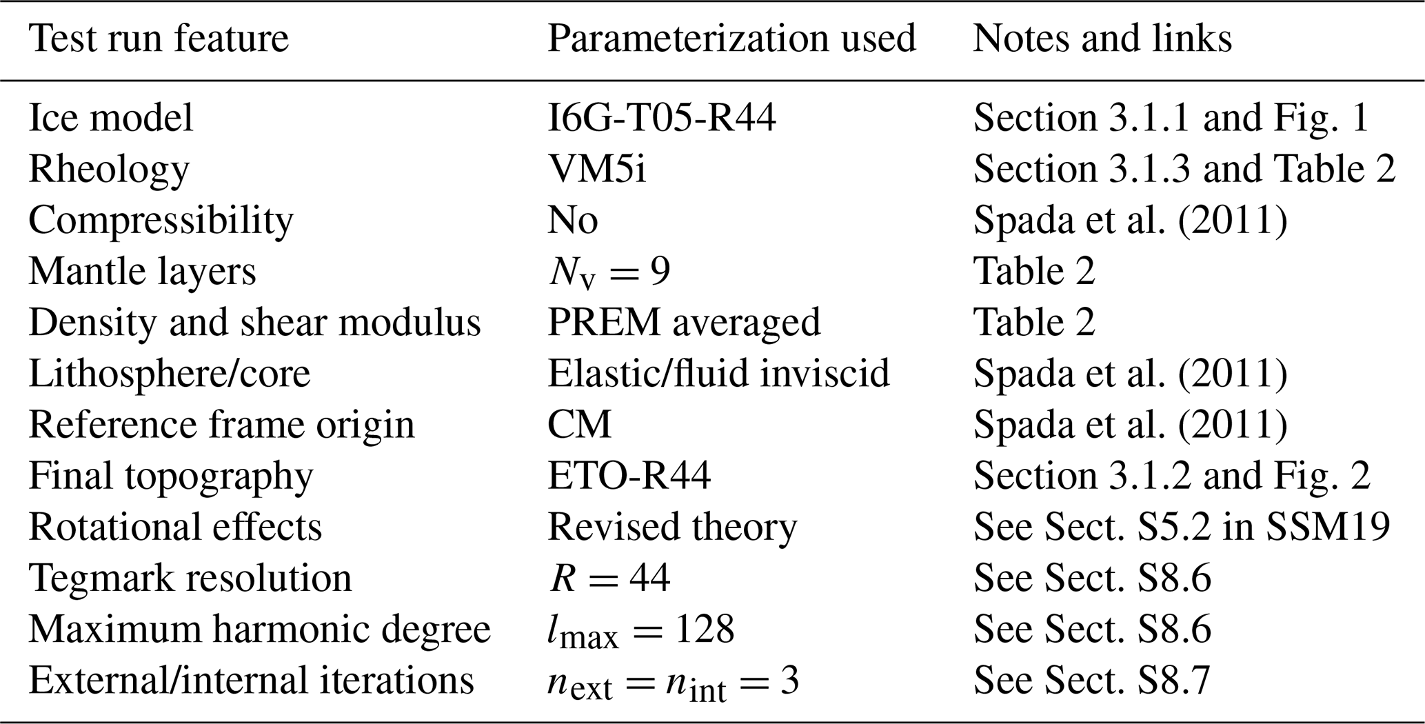
Ice thickness data for model ICE-6G_C have been downloaded from the home page of William R. Peltier in August 2016. The data span the last 26 000 years and are provided on a global latitude–longitude grid (the number of grid points is thus 64 800). In each of the grid cells, the time history of ice thickness is assumed to evolve in a piecewise linear manner, with variable increments of 1.0 or 0.5 kyr. Thus, to fit the SELEN4 default input format, we have first mapped the original thickness data on a spherical equal-area Tegmark grid described in Sect. S8.6 of SSM19. In doing that, we have chosen a resolution parameter R=44, so that the grid consists of P=75 692 pixels (or cells), each with a radius of ∼46 km. The cells' number is thus a bit larger than the number of cells in the original grid. In addition, we have transformed the original time history in a piecewise constant form with a uniform spacing of 0.5 kyr, assuming no glaciation phase prior to deglaciation. Because of the adaptations we have made, the ice model obtained is not an exact replica of ICE-6G_C but a particular realization of it. Hence, to avoid any ambiguity, in the following, it shall be referred to as I6G-T05-R44. Assuming an ice density ρw=931 kg m−3 and that the area of the oceans is fixed to the present value, I6G-T05-R44 holds 206.5 m of equivalent sea level at 26 ka and 75.1 m at present, corresponding to a total eustatic sea-level rise of 131.4 m since the inception of melting (26 ka). The ice thickness of I6G-T05-R44 for a few time frames is shown in Fig. 1.
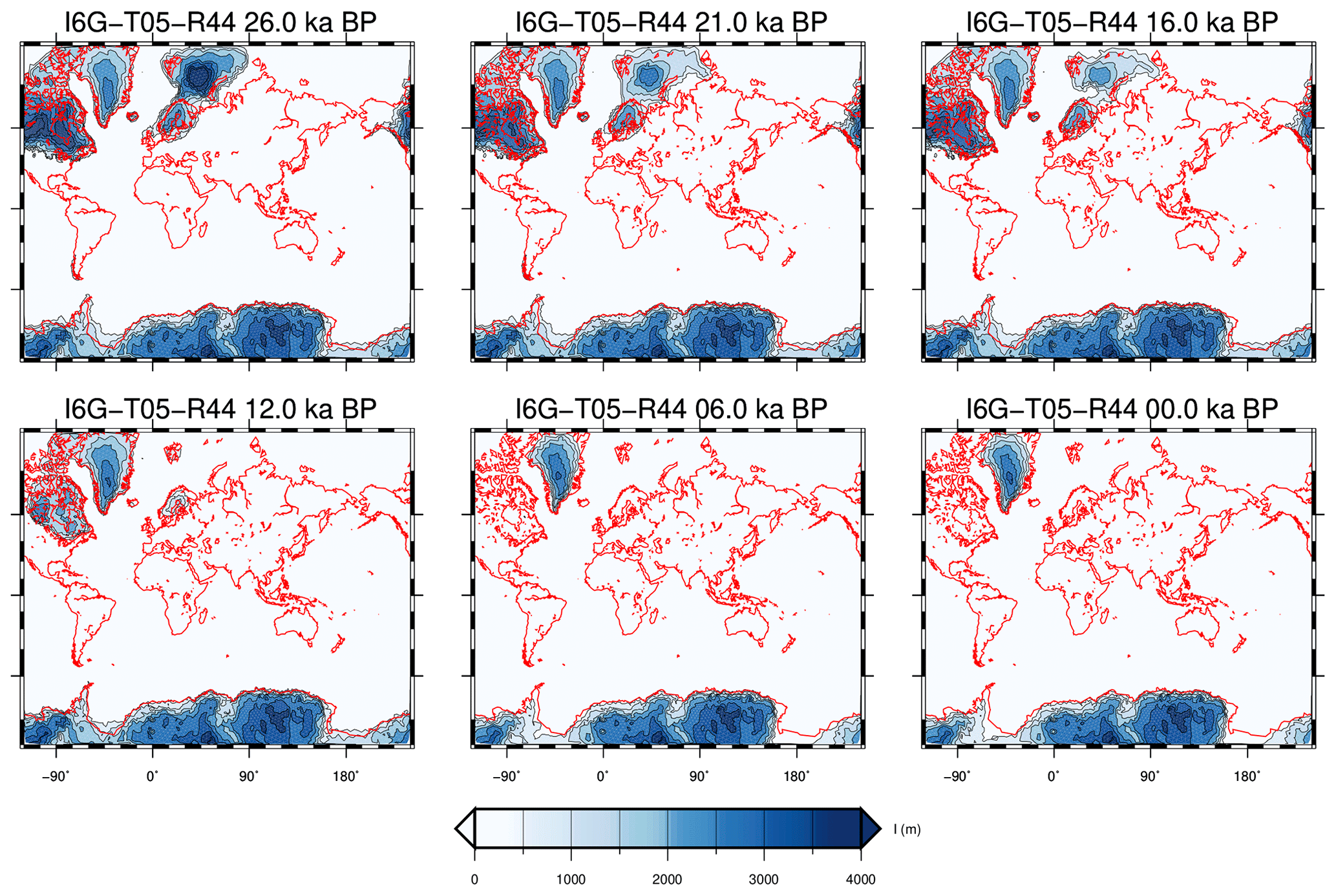
Figure 1Ice distribution according to model I6G-T05-R44, at six different epochs since 26 ka.
The maps are obtained by direct triangulation of the pixelized ice thickness data using the GMT
program pscontour. This and the following figures are drawn using GMT scripts adapted
from those which are available in the output folders of SELEN4 after execution.
3.1.2 Present-day topography
In order to reconstruct the whole history of the Earth's topography and of relative sea level (RSL) since the inception of deglaciation, it is necessary to impose the present relief as a final condition for the sea-level equation (see Peltier, 1994). In this test run, we have utilized the “bedrock version” of the global ETOPO1 dataset (Amante and Eakins, 2009; Eakins and Sharman, 2012) as the final condition, whereas the final condition for the ice thickness is given by the last time frame of I6G-T05-R44. ETOPO1 is distributed on a longitude–latitude grid with a resolution of 1 arcmin (), so that an interpolation of topography on the Tegmark grid has been performed. Note that in regions where small-scale topographic features are present, such as ocean trenches, interpolating a high-resolution relief model on a coarse Tegmark grid may yield inaccurate results. In this case, a different approach should be adopted for the realization of topography, for instance, based on a binning algorithm. Other choices of the final topography are of course possible. For example, in order to ensure the maximum accuracy in Antarctica, the original model, ICE-6G_C (VM5a), employs the Bedmap2 dataset of Fretwell et al. (2013) south of 60∘ S latitude. In SELEN4, there are no restrictions on the choice of the final relief, which is left to the user. In Fig. 2, we show the realization of the modern bathymetry that we have obtained by interpolating ETOPO1 on the same Tegmark grid that we have used for the ice sheets in this test run, which shall be referred to as model ETO-R44 in the following. With SELEN4, other versions of this elevation model are made available, characterized by different spatial resolutions.
Figure 2Present-day relief according to model ETO-R44 used in the test run, obtained from model ETOPO1
by bilinear interpolation on the pixels of the Tegmark grid with resolution R=44, using the GMT
program grdtrack.
3.1.3 Rheological profile
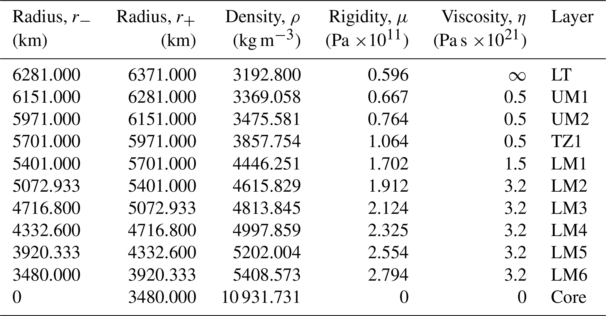
The 11-layer Maxwell rheological profile of the 1-D Earth employed in the test run is shown in
Table 2. For each layer, values of density and of rigidity are obtained by volume averaging the PREM
(Preliminary Reference Earth Model) of
Dziewonski and Anderson (1981), while the viscosity profile is reproduced using the data available in the
Supplement in Peltier et al. (2015). The 90 km thick lithosphere is elastic and the core
is fluid, homogeneous, and
inviscid. Note that the original VM5a profile includes elastic compressibility and reproduces the finely layered PREM
structure (Peltier et al., 2015); since we are employing an incompressible
rheology, in the following, we shall refer to the model in Table 2 as VM5i.
As it includes Nv=9 distinct Maxwell layers in the mantle, for any
given harmonic degree l, the loading Love numbers
(LLNs) and tidal Love numbers (TLNs) for the VM5i model are described
by a spectrum of 4Nv=36 viscoelastic normal modes (see, e.g., Spada et al., 2011).
Since we are not aware of published, community-agreed sets of Love
numbers for a multi-layered compressible viscoelastic model, in the test run we rest on an
incompressible profile, for which agreed results have been obtained by Spada et al. (2011). We remark,
however, that SELEN4 can work with compressible or transient rheologies as well,
provided that LLNs and TLNs in normal-mode form (Wu and Peltier, 1982) are accessible to the user.
Figure 3a and b show the elastic
and fluid values of the LLNs in the range of harmonic degrees for the VM5i model.
The Love numbers are given in a geocentric reference frame
with the origin in the Earth’s
center of mass (CM).
Numerical values of a few relevant LLNs and TLNs are listed in Table 3
and in its caption.
They have been computed by the Love number calculator TABOO (see Spada et al., 2011)
in a multi-precision environment (Smith, 1991; Spada, 2008).

Figure 3Elastic (a) and fluid (b) LLNs as a function of harmonic degree l for the 11-layer rheological VM5i model employed in the test run (see Table 2). It is apparent that for this model asymptotic values are reached, in both cases, for l exceeding values of several hundred. Note that in panel (b), where the fluid LLN for vertical displacement is normalized by (2l+1), the relationship is apparent.
Table 2Density, rigidity, and viscosity profiles adopted in the rheological VM5i model, where abbreviations LT, UM, TZ, and LM stand for lithosphere, upper mantle, transition zone, and lower mantle, respectively. The radii r− and r+ indicate the lower and upper radii of each layer. Some spectral properties of the VM5i model are given in Fig. 3 and Table 3.
3.2 GIA in the past
This section is devoted to the description of some outputs of the SELEN4 test run, concerning the effects of GIA during the whole period after the LGM. These include (i) the predictions of the history of RSL at specific sites, (ii) the time evolution of paleotopography in some regions of interest, and (iii) the excursions of the Earth's pole of rotation forced by GIA.
3.2.1 Relative sea-level curves
Figure 4 shows data (with error bars) and SELEN4 predictions for a small subset of the 392 sites contained in the RSL database of Tushingham and Peltier (1993), hereafter referred to as TP93. In view of its historical importance in the development of GIA studies (e.g., Tushingham and Peltier, 1991, 1992; Melini and Spada, 2019), the TP93 database is available with the SELEN4 package; however, there are no restrictions on the use of other datasets, or simply individual RSL records, if available to the user. Note that ages given in the TP93 database included with SELEN4 are expressed in radiocarbon years and have not been calibrated to calendar years. In Fig. 4, three different configurations, i.e., combinations of parameters R, lmax, next, and nint have been adopted, always assuming next=nint. Results obtained for the three configurations are shown by different colors. The black curves have been obtained using the GIA model described in Sect. 3.1, characterized by the settings R44/L128/I3 (R=44, lmax=128, ). Blue curves have been obtained by configuring SELEN4 with the combination of parameters R100/L512/I5, i.e., increasing the spatial resolution and the number of internal and external iterations in a significant way (a truncation degree is often employed in GIA modeling; see, e.g., Kendall et al., 2005). With this configuration, the pixel radius is reduced to ∼20 km (see Sect. S8.6 and Table S6). Of course, the execution time of SELEN4 increases significantly with respect to the test run, requiring 2.5 d (∼60 h) on a 56-core Intel Xeon E7 Broadwell system. It is apparent that this high-resolution case is providing results substantially matching those of the standard run with R44/L128/I3. Minor differences can be noted in the early stages of deglaciation, which however do not exceed the typical uncertainty on the observed RSL values. These differences are likely to be caused by the significant changes that the topography undergoes in this early phase in the polar regions, which are better captured by increasing the model resolution. Finally, red curves have been obtained for a low-resolution run with R30/L64/I2, whose execution time is 15 min on a 12-core mid-2012 Mac Pro. The curves clearly indicate that computationally inexpensive runs can provide reliable results in the far field of the previously glaciated areas (e.g., at sites 639 and 525), but in the near field (e.g., site 283) they can diverge significantly from both high- and intermediate-resolution results.
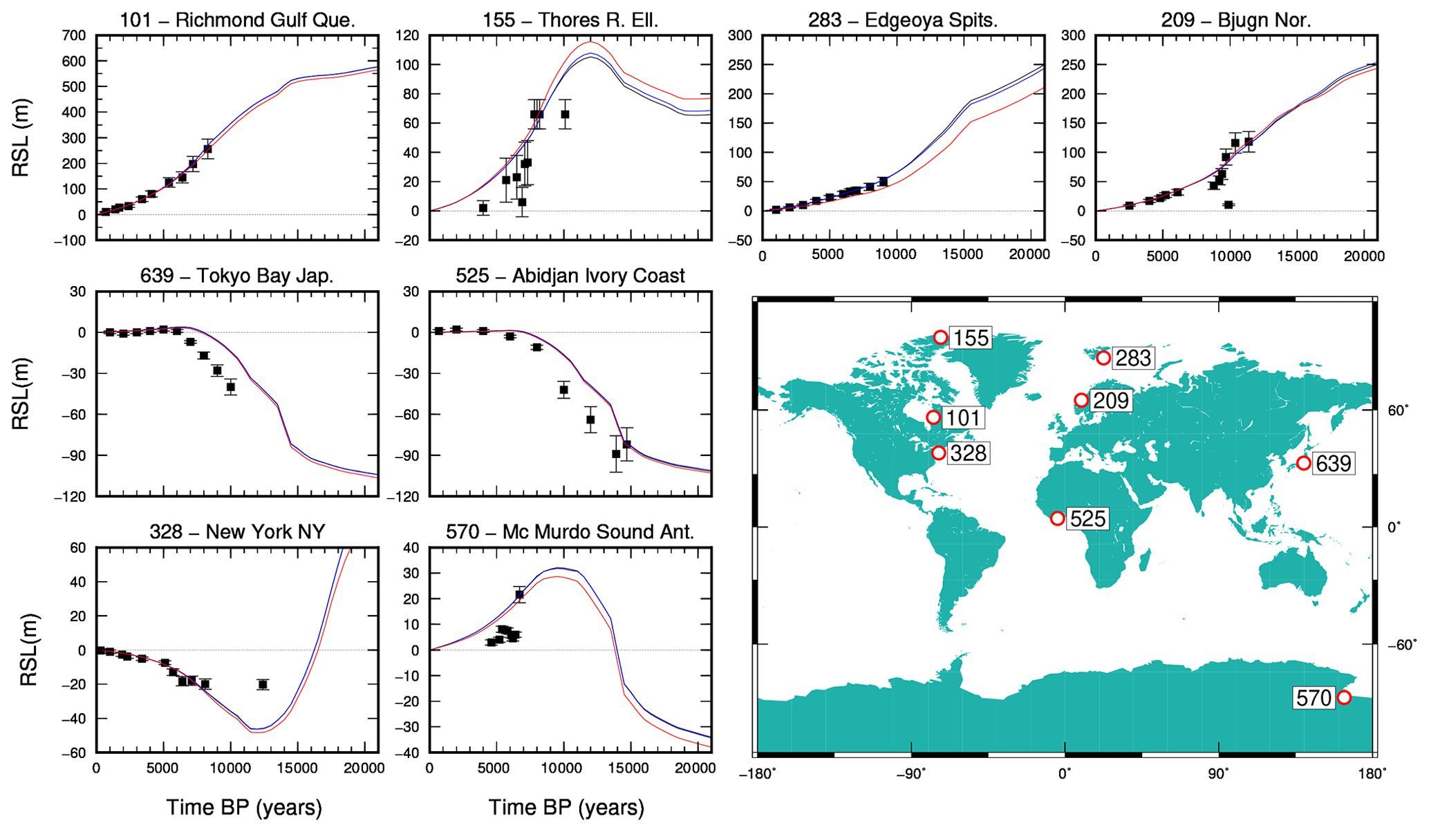
Figure 4RSL data (with error bars) at eight of the 392 sites of the TP93 RSL database. Black curves show the results of the standard test run with configuration R44/L128/I3, the blue ones are for the high-resolution run with R100/L512/I5, while those in red are for a low-resolution configuration with R30/L64/I2. The map shows the location of the RSL sites.
From a visual inspection of Fig. 4, it is apparent that at some sites the best GIA predictions fit very well the observations, like at sites 101 and 283. For others, the trend of the RSL data is captured satisfactorily (see sites 155, 209, and 328), while in some others the fit is quite poor (sites 639, 525, and 570). The identification of the possible sources of the evidenced misfits, which should be measured using rigorous statistical methods after a proper calibration of the ages, is not the purpose of this work. We only note that they do not necessarily stem from limitations of the GIA model adopted, since it is well known that at a specific site tectonic deformations can have an important role (see, e.g., Antonioli et al., 2009, for a significant example), and these are not taken into account when solving the SLE. Similarly, in our formulation of the SLE, we are neglecting the possible effects from the loads exerted by sediments (Dalca et al., 2013). Since the SELEN4 program is open source, the users can modify the code to account for non-glacial loads and change the configuration to determine more suitable combinations of the basic ingredients of GIA modeling, i.e., the history of deglaciation and the rheological layering of the mantle, in order to improve the fit between model predictions and any preferred RSL dataset.
3.2.2 Paleotopography
SELEN4 allows for a gravitationally and topographically self-consistent description of the evolution of sea level along the route highlighted by Peltier (1994) and Lambeck (2004). This implies that SELEN4 can iteratively reconstruct the time evolution of the coastlines and of the OF, in a fashion that is consistent with the gravitational, rotational, and deformational effects induced by deglaciation (for a full account of the theory, the reader is referred to SSM19). These features make the SLE an integral 3-D non-linear equation (Spada, 2017). The importance of the evolution of paleotopography for the development of human culture since the LGM has been pointed out in a number of works (see, e.g., Cavalli-Sforza et al., 1993; Peltier, 1994; Lambeck, 2004; Dobson, 2014, and references therein). Recently, in the context of GIA modeling, Spada and Galassi (2017) have faced the problem of the dynamic evolution of aquaterra, i.e., the land that has been inundated and exposed during the last glacial cycle (Dobson, 1999, 2014), using the same approach adopted in this work.
A standard SELEN4 output is shown in Fig. 5, where the Earth's relief at the LGM is reconstructed in the post-processing phase of SELEN4, according to the solution of the SLE. Note that the figure only shows the bedrock relief at the LGM, which is not what Peltier (1994) has called true paleotopography (PT), which also includes the contribution of ice elevation. The user can easily obtain maps of the full PT merging maps like that shown in Fig. 5 with those of Fig. 1. Light blue areas across the polar regions covered by thick ice at the LGM correspond to places where the ice was grounded below sea level in that epoch. In SELEN4, it is also possible to visualize the full time evolution of the OF in order to better appreciate, for example, the spatiotemporal distribution of the ice shelves, which cannot be seen in this paleotopography map. At the global scale, the major land masses that were exposed at the LGM are clearly visible, as evidenced by the low-elevation green areas; these include Beringia, Sundaland, Patagonia, Sahul, Doggerland, and the East Siberian Arctic Shelf. Using GIA models, the time evolution of these land masses has been investigated in an a number of papers, also in view of the important implications on the dispersal of modern humans. For specific case studies, the reader is referred to the works of Peltier and Drummond (2002), Lambeck (2004), Klemann et al. (2015), Spada and Galassi (2017), and references therein.
Figure 5Sample SELEN4 output of the global relief at the LGM (21 ka), according to the test run with R44/L128/I3, where topography ETO-R44 of Fig. 2 has been used as a final condition for the SLE.
By increasing the spatial resolution, SELEN4 can also be employed to resolve the past sea-level variations on a regional scale. As a specific case study, we consider the Mediterranean Sea. The history of RSL in the Mediterranean Sea has been the subject of various investigations, stimulated by the amount of high-quality geological, geomorphological, and archeological indicators in the region (see, e.g., Lambeck and Purcell, 2005; Antonioli et al., 2009; Evelpidou et al., 2012; Vacchi et al., 2016; Roy and Peltier, 2018, and references therein). Since on the global scale of Fig. 5 the details of the paleotopography in this area are difficult to visualize, we have used the outputs of the high-resolution run with settings R100/L512/I5, already exploited in Sect. 3.2.1. The results are shown in the map of Fig. 6, where paleotopography is shown at 26 ka. The vastly exposed continental shelf of Tunisia (Mauz et al., 2015) and the northern Adriatic Sea (Lambeck and Purcell, 2005) are now clearly visible, along with other smaller-scale regions where the topography has seen significant changes during the last deglaciation (Lambeck, 2004; Purcell and Lambeck, 2007).
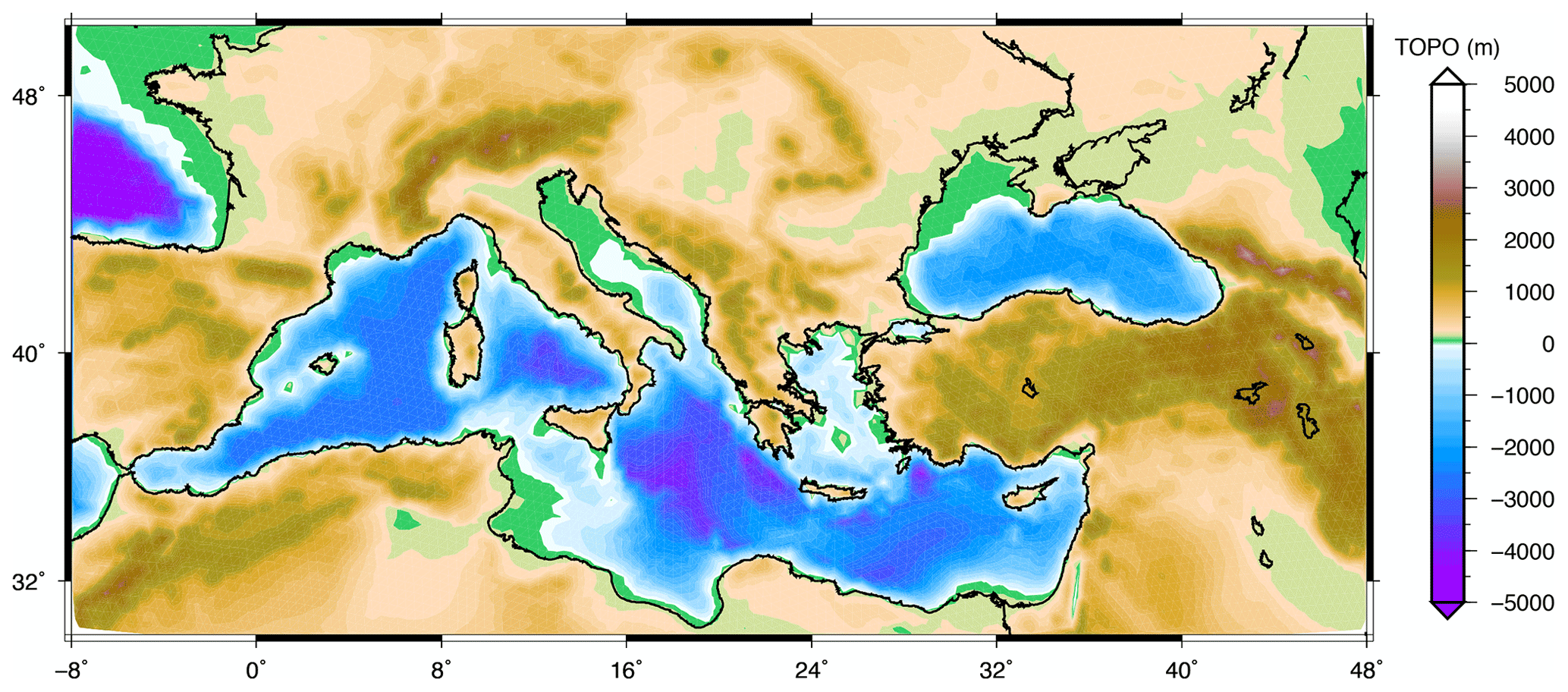
Figure 6Paleotopography of the Mediterranean Sea and the Black Sea at 26 ka, obtained by a high-resolution SELEN4 run with configuration R100/L512/I5, in order to highlight the exposed lands in detail.
3.2.3 Polar motion
With SELEN4, three configurations are possible in which rotational effects on GIA are dealt with in different manners. First, these effects can be simply ignored, as it is done in the classical FC76 GIA theory. However, when rotational effects are taken into consideration, this can be done in two different ways, i.e., either following the traditional rotation theory (Milne and Mitrovica, 1998; Spada et al., 2011) or a revised rotation theory proposed by Mitrovica et al. (2005) and Mitrovica and Wahr (2011). The reader is referred to the literature for a detailed presentation of the two theories and to Sect. S5.2 for a brief account. We also refer to Martinec and Hagedoorn (2014) for a general formulation dealing with rotational effects in GIA modeling. Here, it is useful to mention that in the traditional treatment the long-term response of the Earth is evaluated assuming that the lithosphere is characterized by a finite elastic strength, while in the revised theory the equilibrium rotational shape is, more realistically, only based on the viscous properties of the planet. Furthermore, the long-term extra flattening due to mantle dynamics is properly accounted for. We remark that in both cases the fast Chandler wobble component of polar motion is filtered out from the Liouville equations, because the timescales of GIA largely exceed the Chandler wobble period (∼14 months; see, e.g., Lambeck, 1980). The implications for the GIA response of the new theory are quite significant, as illustrated in detail by Mitrovica et al. (2005) and Mitrovica and Wahr (2011) and shown in Fig. 7.
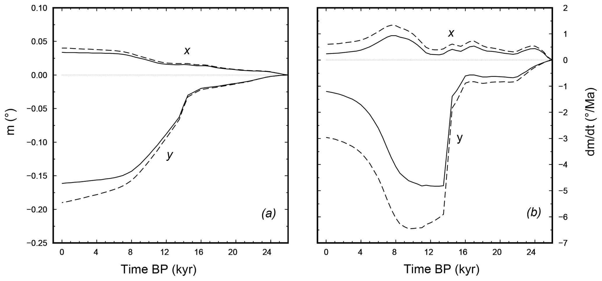
Figure 7Cartesian components of polar motion along the axes x and y (a) and their time derivatives (b) as a function of time since the beginning of deglaciation for the test run with configuration R44/L128/I3. The x axis points along the prime meridian and the y points to 90∘ E. Dashed and solid curves show results for the traditional and for the revised rotational theories, respectively. The steep change in the y components at ∼14 ka is forced by the inertia variations due to the occurrence of the meltwater pulse 1A (MWP-1A).
Solid curves in Fig. 7 show the evolution of the polar motion components (mx,my) and their rates of change in response to GIA, obtained by solving the Liouville equations in the test run, in which the revised rotation theory is employed. Dashed curves show results obtained with the traditional theory. As the x and y components of polar motion are conventionally measured along the Greenwich meridian and 90∘ E, respectively, Fig. 7a indicates that since the inception of deglaciation, the displacement of the pole has been roughly in the direction of the Hudson Bay, consistent with the seminal results of Sabadini and Peltier (1981). The two theories predict similar evolutions of the pole of rotation, which according to Fig. 7a has been displaced by ∼18 km on the Earth's surface by the glacial readjustment process since 26 ka. We note that at the time of the rapid melting episode known as meltwater pulse 1A (MWP-1A, between 14.3 and 12.8 ka; see, e.g., Blanchon, 2011), a sudden variation in the my component of polar motion had occurred but no changes could be observed on mx. When the rates of polar motion are considered in Fig. 7b, differences between the predictions of the two rotations theories are more apparent. In particular, the present-day (0 ka) rates of polar motion are found to be ∼1 and ∼3∘ Ma−1 for the revised and the traditional theories, respectively, which fits the predictions of Mitrovica and Wahr (2011) and confirms that the traditional theory largely overestimates the effects of GIA on polar motion. We note also that MWP-1A has caused a remarkable acceleration of polar motion, with a rate as large of ∼5∘ Ma−1 near the end of the pulse; this value exceeds the rate of polar motion observed since the year 1900 by a factor of ∼5 (see, e.g., Dickman, 1977).
3.3 GIA at present
In this section, we describe further outputs of the SELEN4 test run, focusing on the effects of GIA at the present time. In particular, we consider (i) the global pattern of the so-called GIA fingerprints, (ii) predictions of the rate of sea-level change at tide gauges, and (iii) the time variations of the Stokes coefficients of the Earth's gravity field induced by GIA.
3.3.1 GIA fingerprints
Figure 8 shows another standard output of SELEN4, i.e., the present-day rates of variation of four fundamental quantities associated with GIA, obtained for the test run. These are relative sea-level change (; Fig. 8a), vertical displacement of the crust (; Fig. 8b), absolute sea level (; Fig. 8c), and geoid height (; Fig. 8d). Generalizing the definition of sea-level fingerprint introduced by Plag and Jüettner (2001) in the context of contemporary ice mass changes, these have been referred to as GIA fingerprints by Spada and Melini (2019). The spatial variability of the GIA fingerprints reflect the effects of deformation, gravitational attraction, and rotation within the system composed by the solid Earth, the oceans, and the ice sheets (Clark et al., 1978; Mitrovica and Milne, 2002). In view of their importance on the interpretation of ground-based (King et al., 2010) or satellite geodetic observations (Peltier, 2004) and of tide gauge secular trends (e.g., Spada and Galassi, 2012; Wöppelmann and Marcos, 2016), their properties have been the subject of various investigations during last decade (see, e.g., Mitrovica et al., 2011; Tamisiea, 2011; Spada and Galassi, 2015; Spada, 2017; Husson et al., 2018; Melini and Spada, 2019; Spada and Melini, 2019).
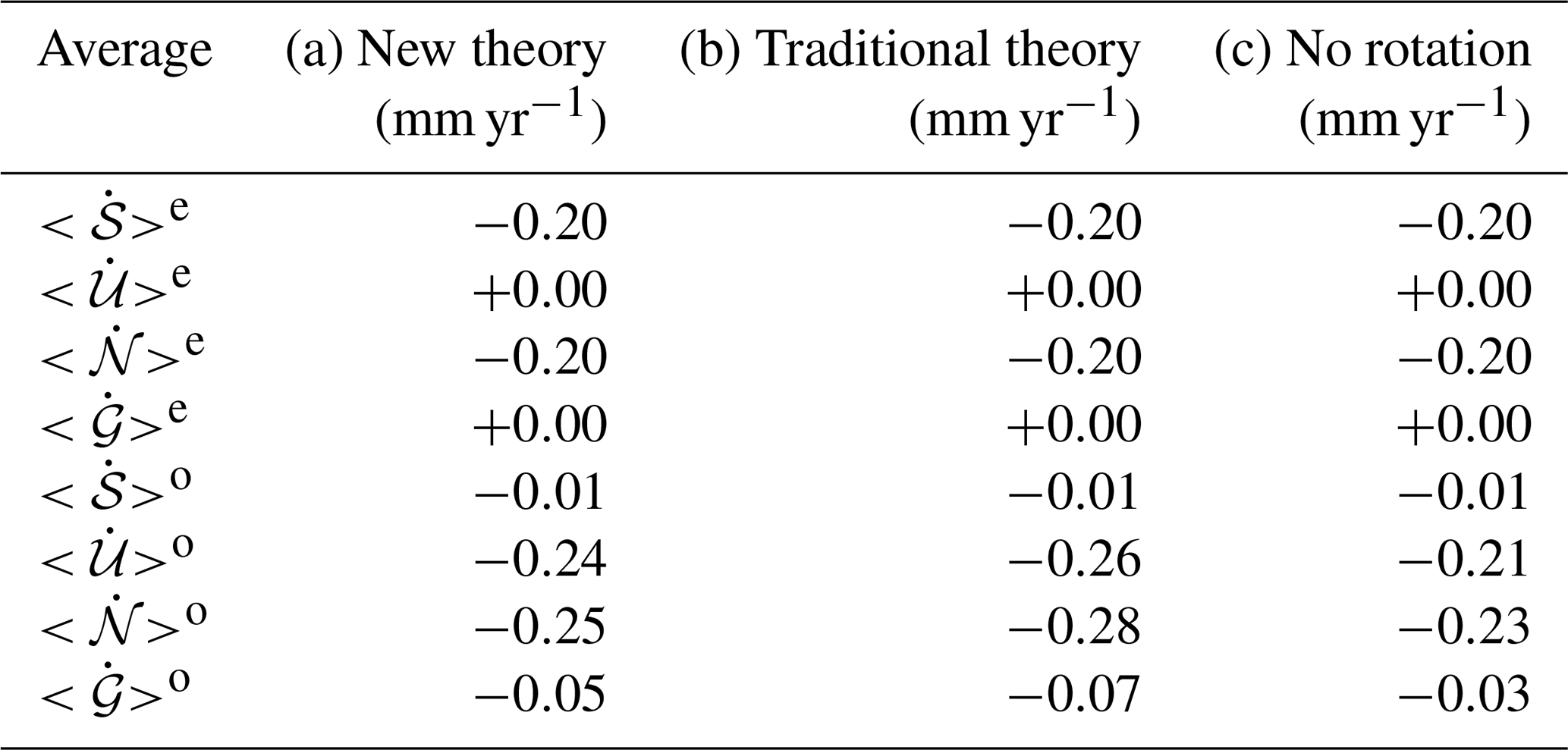
It should be remarked that the four fingerprints shown in Fig. 8 are not independent of one another. In particular, the SLE gives according to Eq. (21). Furthermore, , where c is the FC76 constant (see Sect. S2.4 in SSM19). The two relationships above hold, regardless of the particular combination of rheology and ice model employed, and the preferred rotation theory adopted. However, the patterns of the GIA fingerprints and the numerical value of are model dependent. Other interesting results hold for the spatial averages of the fingerprints, which reflect some physical aspects of GIA (Spada, 2017; Spada and Melini, 2019) and are useful to correct geodetic observations from the effects of deglaciation (e.g., Spada and Galassi, 2015). In Table 4, we summarize the numerical values of whole Earth surface averages (denoted by the symbol ) and ocean averages () of the GIA fingerprints in the test run. In addition, we have also executed SELEN4 adopting the traditional rotation theory and neglecting rotational effects, and the corresponding averages are shown in Table 4 as well. We note that by virtue of mass conservation, (see Sects. S4.3 and S6.2), regardless of the rotation theory adopted, and as a consequence . We also note that the numerical value of , commonly employed to correct the altimetry observations of absolute sea-level change for the effects of GIA, is in fair agreement with predictions from state-of-the-art GIA models (e.g., Church et al., 2013; Spada and Galassi, 2015; Spada, 2017). Notably, is not very sensitive to the choice of the rotation theory. Since model I6G-T05-R44 assumes that melting of the major ice sheets ceased ∼4000 years ago, the small value of only reflects ongoing changes in the area of the oceans due to GIA. In the FC76 fixed-shoreline approximation, would be identically zero by virtue of the mass conservation principle (see, e.g., Spada, 2017; Spada and Melini, 2019).
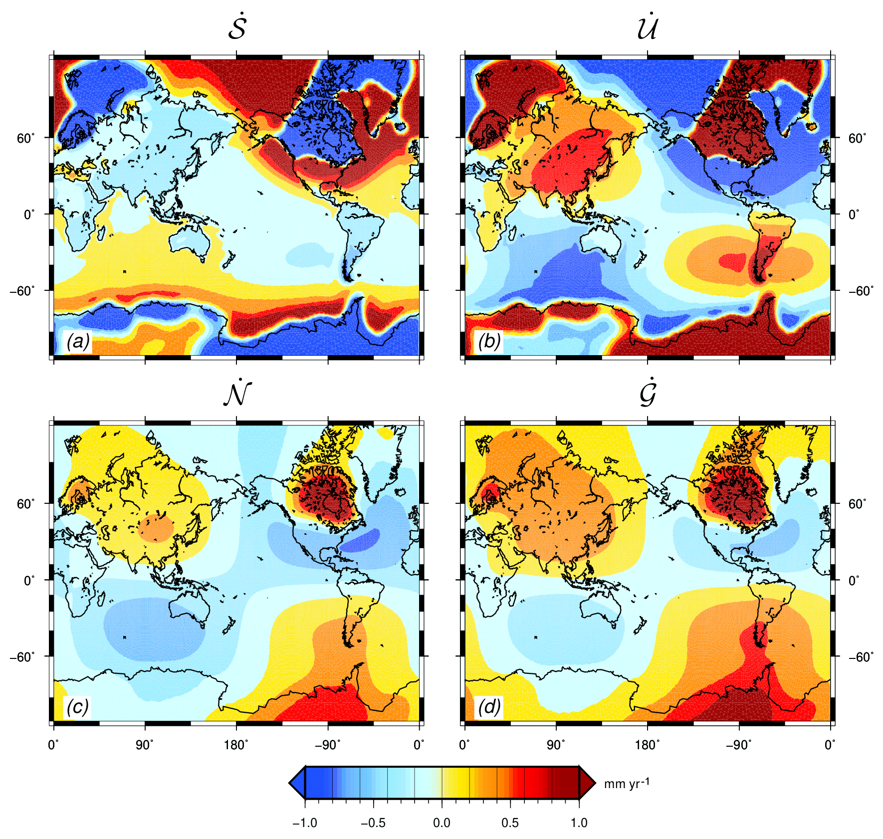
Figure 8Present-day GIA fingerprints obtained for the test run with R44/L128/I3. Note that the color table is saturated in a narrow interval. The effects of Earth rotation, evaluated according to the revised rotation theory, can be well discerned for and , with the characteristic high-amplitude lobes with a harmonic degree l=2 and order m=1 symmetry (Spada and Galassi, 2015). Spatial averages of these maps are given in Table 4. Min/max values for , , , and , after rounding the SELEN4 outputs to one decimal figure, are , , , and in units of mm yr−1, respectively.
Table 3Numerical values of the LLNs for the VM5i rheological model (see Table 2) for some harmonic degrees l. Here xe and xe are abbreviations for x×10e and , respectively. Note that, for this model, the elastic TLNs of degree l=2 are , while the fluid values are = .
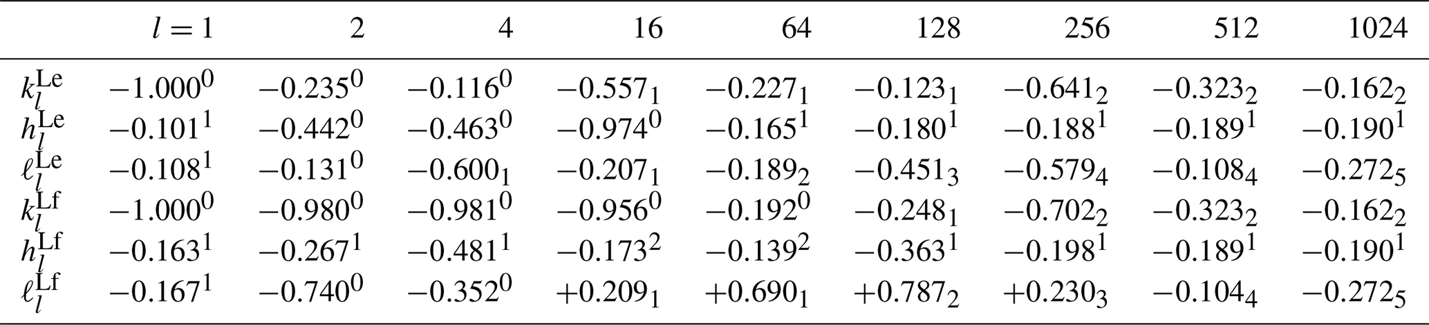
Table 4Whole Earth and ocean averages of the GIA fingerprints according to the test run based upon the new rotation theory (column a), and the traditional theory (column b). In column (c), we also consider the case when no rotational effects are taken into account. In all the computations, we have adopted the combination R44/L128/I3. Note that , where c is the FC76 constant. In this table, the SELEN4 outputs are rounded to two significant figures.
3.3.2 GIA at tide gauges
Estimating global mean sea-level rise in response to climate change requires correcting tide gauge records for the effects of GIA. Since the late 1980s, with the awareness of global warming and the availability of numerical solutions of the SLE (Peltier and Tushingham, 1989), GIA corrections have been routinely applied to the observed trends of sea level (for a review, see Spada and Galassi, 2012; Spada et al., 2015; Wöppelmann and Marcos, 2016). However, since GIA models are progressively improved to provide a better description of reality, corrections at tide gauges are not given once and for all (Kendall et al., 2006; Tamisiea, 2011; Melini and Spada, 2019). Furthermore, new constraints from past sea level or modern geodetic observations have permitted gradual refinements (either by formal inverse methods or simply by trial and error) of the two basic ingredients of GIA modeling, i.e., the Earth rheological profile and the history of deglaciation since the LGM. Uncertainties in modeling are significant (Melini and Spada, 2019), which constitutes an additional motivation to improve the approach to GIA.
In Table 5, we show SELEN4 predictions for at a few tide gauges for the test run and other possible configurations as well. Here, we only show results for the 23 sites that have been considered by Douglas (1997) in his redetermination of global sea-level rise, which obey specific criteria that make them suitable to represent the trend of secular sea-level rise. The sites chosen by Douglas (1997) are located in the periphery of the regions covered by thick ice sheets at the LGM, since GIA predictions at sites formerly beneath the ice sheets are expected to be more affected by uncertainties in GIA modeling. This has been recently confirmed by Melini and Spada (2019). The post-processing phase of SELEN4 can be configured to handle any properly formatted input dataset with coordinates of geodetic points of interest, where all the variables considered in Fig. 8 can be evaluated. This can be useful, for instance, to estimate the effects of GIA on vertical movements at specific GPS points (Serpelloni et al., 2013). Modules for the computation of horizontal displacements shall be included in future releases. Comparing column (d) with (b) and (c) (all these runs are characterized by the intermediate-resolution configuration R44/L128/I3), we note that rotational effects are important at tide gauges; however, from columns (b) and (c), we also note that differences between the revised and the traditional rotation theories generally do not exceed the 0.1 mm yr−1 level at the tide gauges considered here. Comparing outputs in column (b) with the high-resolution run in column (a), we note maximum differences of 0.03 mm yr−1, which further confirms the reliability of the test run.
Table 5Present-day rates of sea-level change at the 23 Douglas (1997) tide gauges for the test run of SELEN4 (column b) and for other configurations. Results based upon the original implementation of model ICE-6G_C (VM5a) are reproduced in column (e). The average rate is also shown in the bottom line. The SELEN4 outputs have been rounded to two significant figures.
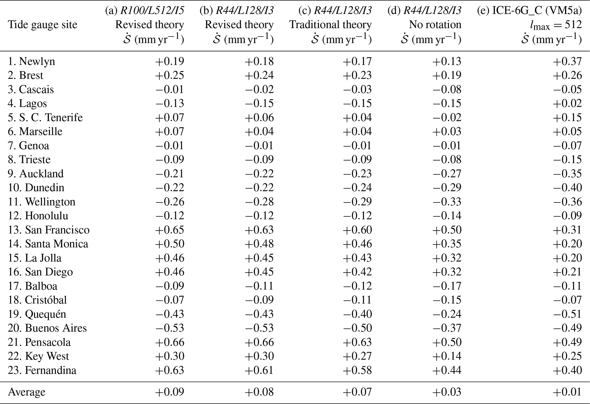
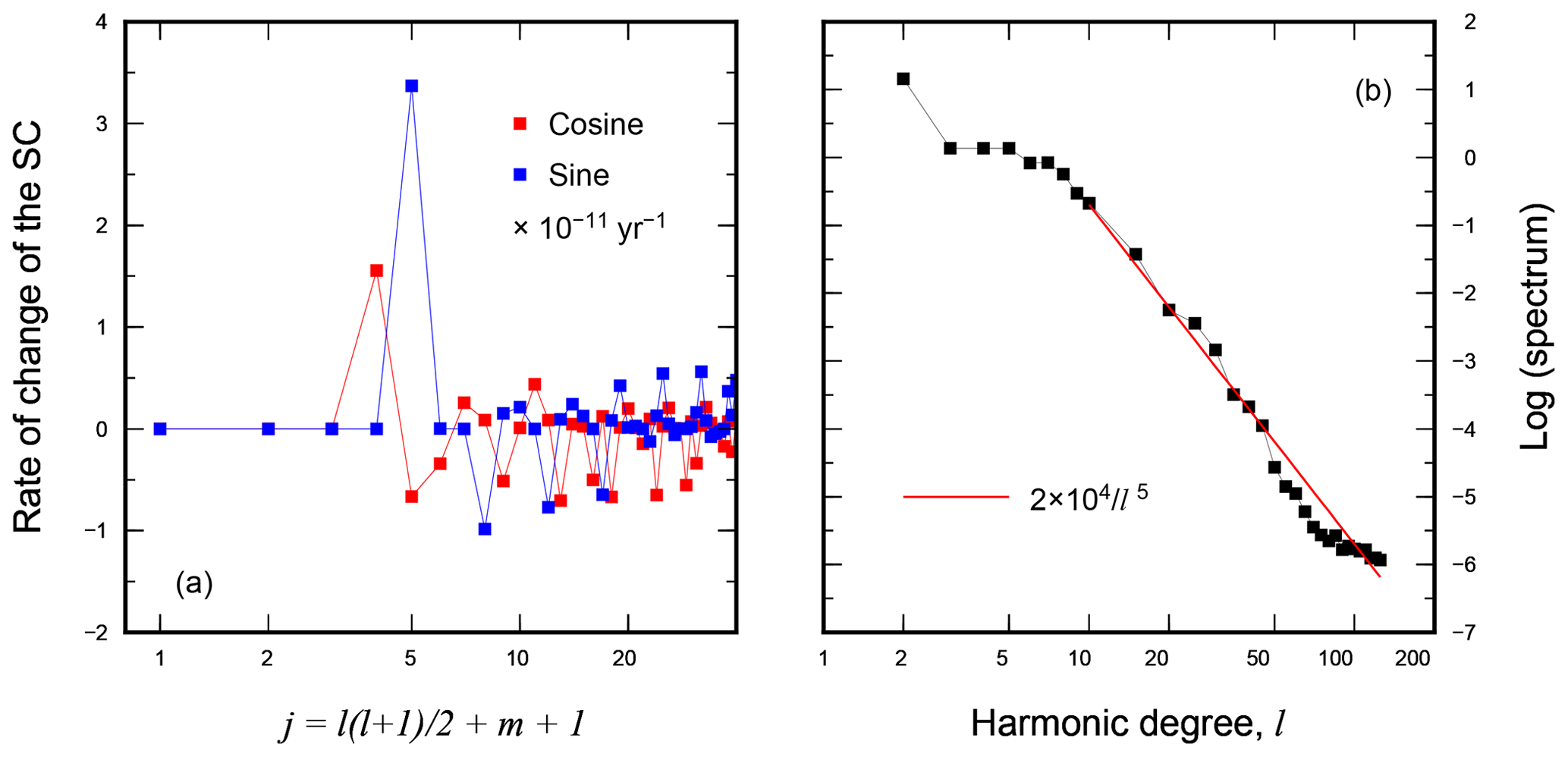
Figure 9Present-day rate of change of the low harmonic degree (l≤6) Stokes coefficients obtained for the test run of SELEN4 (a) and their full spectrum extended to harmonic degree (b). The solid line in panel (b) represents the power law that best fits the spectrum, in the least squares sense, for l≥10.
Comparing the high-resolution results in Table 5 (R100/L512/I5, column a) with those obtained using the ICE-6G_C (VM5a) model in the original implementation of W. R. Peltier (see http://www.atmosp.physics.utoronto.ca/~peltier/data.php, last access: 6 June 2019), reported in column (e), we note a fair agreement between the two model predictions. The two sets of predictions have the same sign with the only exception of Lagos. The differences between the values obtained with R100/L512/I5 and the original implementation, ICE-6G_C (VM5a), are generally close to 0.2 mm yr−1 or slightly larger. The values of averaged over the tide gauges differ, but they are both <0.1 mm yr−1. More significant differences in the values are however apparent when we compare model predictions for sites located in the polar regions beneath the former ice sheets, which are not considered in Table 5. At these locations, the expected values are of the order of several mm yr−1, due to the large isostatic disequilibrium still associated with ice unloading. For example, at the tide gauge of Stockholm, we obtain a rate of −4.44 mm yr−1 for the high-resolution run R100/L512/I5, while in the original ICE-6G_C (VM5a) implementation, the rate is −3.75 mm yr−1. To better evaluate the meaning of these differences, it is worth noting that they largely exceed the typical 2σ uncertainty in the observed rates, which according to Spada and Galassi (2012) is never larger than 0.3 mm yr−1 (see their Table 2). We have also ascertained that misfits of the order of 1 mm yr−1 are not uncommon in other high-latitude sites of both hemispheres. Tracing the origin of the discrepancies in the two sets of GIA predictions (and therefore in the whole set of the GIA geodetic fingerprints considered in Fig. 8) is not easy at this stage and would demand a detailed model intercomparison study like those performed in the GIA community by Spada et al. (2011) and Martinec et al. (2018). We can, however, guess that the misfit between the two sets of GIA predictions stems from the different discretizations of the ice time histories, from the effects of mantle compressibility, and possibly from the different rotation theories adopted.
3.3.3 Stokes coefficients of the gravity field
In Fig. 9, we study the present-day rates of change of the variations of Stokes coefficients () induced by GIA, computed in the test run with R44/L128/I3. These quantities represent the coefficients of the expansion of the gravity potential variation in series of spherical harmonics; hence, they contain information upon the response of the Earth to surface loading and to movements of the axis of rotation. In SELEN4, we use a real, fully normalized representation for the Stokes coefficients, following GRACE conventions for spherical harmonics (see, in particular, Bettadpur, 2018 and Sect. S8.9 in SSM19). However, it is important to note that in Fig. 9, the Stokes coefficients also include the direct effect of the Earth's rotation, associated with the change in centrifugal potential, on the TLNs of harmonic degree l=2 (i.e., they account for the “δ(t)” term in “”; see Eq. S173); hence, the rates we have computed are not directly comparable with the GRACE rates. In fact, since in its orbit GRACE is not physically connected with the Earth, it cannot be influenced by the direct rotational effect (the whole issue has been the subject of discussion a few years ago; see Chambers et al., 2010; Peltier et al., 2012; Chambers et al., 2012). The user of SELEN4, however, can supply the program with a rotation response function (𝒢rot) that does not include the direct term in order to produce GRACE-compliant Stokes coefficients which are only indirectly affected by the Earth's rotation.
The fully normalized cosine (squares) and sine (circles) coefficients () are shown in Fig. 9a only for harmonics with degree l≤6. The dominance of the degree 2 coefficients is apparent, which reflect the symmetries of the fingerprint in Fig. 8d. We note that since , where is the absolute sea-level fingerprint in Fig. 8c and c is the FC76 constant (see Eq. 22), the Stokes coefficients for and for coincide for l≥2. For reference, the numerical values of the degree l=2 coefficients obtained in the test run are , , , , and in units of 10−11 yr−1; the modulus of all other coefficients is <1 in these units. To better visualize the decay of the Stokes coefficients with increasing l, in the diagram of Fig. 9b, we show the harmonic spectrum defined in Sect. S8.9 (see Eq. S477). By inspection of the spectrum plot, it is now apparent that the energy contained in the degree l=2 harmonic component exceeds by at least 1 order of magnitude all those with l≥3. After a plateau that indicates a substantial power equipartition in the range of harmonic degrees , the spectrum clearly shows a red character and decays very rapidly, closely following a power law (solid line). This result is consistent with those obtained by Spada and Galassi (2015), although they have used a simplified GIA model with fixed shorelines and the traditional rotation theory. They confirm that, for l≥3, the power contained in the GIA-induced regional variations in absolute sea level is negligible when compared with the spectrum observed during the altimetry era.
We have presented an updated version of the SLE solver SELEN, which was
originally introduced by Spada and Stocchi (2007) and principally meant as a tool for students.
Along with a condensed theory background and the basic features of the new program,
we have provided a step-by-step description of the outcomes of a medium-resolution test
run that requires modest computing resources. However, the run
accounts for an up-to-date description of the time history of melting since the LGM and a realistic rheological profile,
being based upon a realization of the ICE-6G_C (VM5a) model of Peltier et al. (2015).
The outputs of the test run, which cover different temporal scales, have been briefly discussed
in order to appreciate some of the possible geodynamical implications. Outputs of
a high-resolution test run have been also presented to illustrate the effects of spatial
and harmonic resolution on some GIA predictions.
With respect to the original version of the code, two major improvements have been made in SELEN4. The first is represented by an increased realism in the description of the GIA process. Indeed, now the program accounts for the migration of the shorelines and for the rotational feedback on sea-level change, which enable a fully topographically and gravitationally self-consistent modelization, in the sense defined by Peltier (1994). Furthermore, SELEN4 can be configured assuming two different rotation theories or even excluding rotational effects. The second improvement is in terms of usability, efficiency, and versatility, and covers various aspects. First, the solution of the SLE is now performed by a single Fortran program unit, leaving to a flexible and customizable post-processor the computation of various outputs encompassing the broad spectrum of the GIA phenomenology. Second, on modern multi-core systems, SELEN4 can take advantage of multi-threaded parallelism to speed up the most computationally intensive portions of the code. The reader can find details about computational aspects as execution time and code parallelism in Sect. S8.7 of SSM19. Third, the user can easily customize the time evolution of the surface load and the rheological layering of the Earth providing precomputed loading and tidal Love numbers. Last, SELEN4 comes with a user guide and with a fully detailed theory background in a supplement, which is particularly meant to illustrate the basic concepts of GIA to young scientists or colleagues and to allow transparency and reproducibility.
In the framework of a recent benchmarking initiative (Martinec et al., 2018), a preliminary version of the new program has been successfully tested against other independently developed SLE solvers, in the particular case in which rotational effects are not taken into account and assuming simplified surface loads. The version of SELEN4 that is distributed with the present work reproduces the numerical results published in Martinec et al. (2018), if the code is configured with the parameters employed in the benchmark exercise. After it was progressively developed in various interim versions, SELEN4 has now been released to the GIA and to the global geodynamics community as an open-source tool.
SELEN4 is available from Zenodo at https://zenodo.org/record/3520451 (https://doi.org/10.5281/zenodo.3520451; Spada and Melini, 2019) and from the Computational Infrastructure for Geodynamics (CIG) at http://geodynamics.org/cig/software/selen (Spada and Melini, 2015). SELEN4 is released under a three-clause BSD license (for details, see https://opensource.org/licenses/BSD-3-Clause, last access: 26 November 2019). The ice history data for ICE-6G (VM5a) were downloaded from http://www.atmosp.physics.utoronto.ca/~peltier/data.php (last access: 20 April 2019). The ETOPO1 model was obtained from https://www.ngdc.noaa.gov/mgg/global/ (last access: 26 February 2019).
The supplement related to this article is available online at: https://doi.org/10.5194/gmd-12-5055-2019-supplement.
GS and DM both contributed to the design and implementation of the research, to the analysis of the results, and to the writing of the manuscript. The Supplement was written by GS, with the support of DM. The code was progressively developed by GS and DM, who edited the user guide and the online version of the code.
The authors declare that they have no conflict of interest.
We thank Daniela Riposati from the INGV Laboratorio Grafica e Immagini for drawing the SELEN logo.
We thank Max Tegmark for having made available his pixelization routines, which have had
an essential role in the development of SELEN
(see https://space.mit.edu/ home/ tegmark/ isosahedron.html, last access: 26 November 2019).
We also thank Mark Wieczorek for distributing the SHTOOLS (Spherical Harmonics Tools)
to the community (https://shtools.oca.eu/shtools, last access: 26 November 2019).
Some of the figures have been drawn using the Generic Mapping Tools (GMT)
of Wessel and Smith (1998).
We are indebted to all the colleagues who
participated in the various stages of the glacial isostatic adjustment and sea-level
equation benchmark activities, namely Valentina Barletta, Paolo Gasperini, Thomas James,
Matt King, Samuel Kachuck, Volker Klemann, Björn Lund, Zdenek Martinec, Riccardo Riva, Karen Simon, Yu Sun,
Bert Vermeersen, Wouter van der Wal, and Detlef Wolf; (see Spada et al., 2011; Martinec et al., 2018).
A special acknowledgement goes to Florence Colleoni for help in the code implementation and to Francesco Mainardi
for advice on the theory of linear viscoelasticity.
We are also indebted to Michael Bevis and Erik Ivins for
encouragement and advice. We thank Glenn Milne for discussion about the meaning of the
GIA fingerprints.
We are grateful to Volker Klemann, Samuel Kachuck, and Geruo A for their constructive review and advice, and Meike Bagge and
Evan Gowan for
their very helpful comments. We have greatly benefitted from the discussion, advice, and encouragement from all the teachers and
students of the 2019 GIA Training School (26–30 August 2019, Lantmäteriet, Gävle, Sweden).
Raffaello Mascetti
has patiently revised the manuscript during various stages of its development,
also providing invaluable inspiration.
Giorgio Spada is funded by a FFABR (Finanziamento delle Attività Base di Ricerca) grant of MIUR (Ministero dell'Istruzione, dell'Università e della Ricerca) and by a research grant of DiSPeA (Dipartimento di Scienze Pure e Applicate) of the Urbino University “Carlo Bo”.
This paper was edited by Steven Phipps and reviewed by Volker Klemann, Geruo A, and Samuel Kachuck.
Adhikari, S., Ivins, E. R., and Larour, E.: ISSM-SESAW v1.0: mesh-based computation of gravitationally consistent sea-level and geodetic signatures caused by cryosphere and climate driven mass change, Geosci. Model Dev., 9, 1087–1109, https://doi.org/10.5194/gmd-9-1087-2016, 2016. a
Amante, C. and Eakins, B.: ETOPO1 Arc-Minute Global Relief Model: Procedures, Data Source and Analysis, Tech. rep., 2009. a
Antonioli, F., Ferranti, L., Fontana, A., Amorosi, A., Bondesan, A., Braitenberg, C., Dutton, A., Fontolan, G., Furlani, S., Lambeck, K., Mastronuzzi, G., Monaco, G., Spada, G. and Stocchi, P.: Holocene relative sea-level changes and vertical movements along the Italian and Istrian coastlines, Quatern. Int., 206, 102–133, 2009. a, b
Bamber, J., Riva, R., Vermeersen, B., and LeBrocq, A.: Reassessment of the potential sea-level rise from a collapse of the West Antarctic Ice Sheet, Science, 324, 901–903, 2009. a
Bettadpur, S.: Level-2 gravity field product user handbook, The GRACE Project, Jet Propulsion Laboratory, Pasadena, CA, 2003, available at: https://podaac-tools.jpl.nasa.gov/drive/files/allData/grace/docs/L2-UserHandbook_v4.0.pdf (last access: 26 November 2019), 2018. a
Bevis, M., Melini, D., and Spada, G.: On computing the geoelastic response to a disk load, Geophys. J. Int., 205, 1804–1812, 2016. a, b
Blanchon, P.: Meltwater pulses, in: Encyclopedia of Modern Coral Reefs: Structure, form and process, Encyclopedia of Earth Science Series, Springer, 683–690, available at: http://unam.academia.edu/PaulBlanchon/Papers (last access: 26 November 2019), 2011. a
Cavalli-Sforza, L. L., Menozzi, P., and Piazza, A.: Demic expansions and human evolution, Science, 259, 639–639, 1993. a
Cazenave, A. and Llovel, W.: Contemporary sea level rise, Annu. Rev. Mar. Sci., 2, 145–173, 2010. a
Cazenave, A., Dominh, K., Guinehut, S., Berthier, E., Llovel, W., Ramillien, G., Ablain, M., and Larnicol, G.: Sea level budget over 2003–2008: A reevaluation from GRACE space gravimetry, satellite altimetry and Argo, Global Planet. Change, 65, 83–88, 2009. a
Chambers, D., Wahr, J., Tamisiea, M., and Nerem, R.: Ocean mass from GRACE and glacial isostatic adjustment, J. Geophys. Res., 115, B11415, https://doi.org/10.1029/2010JB007530, 2010. a, b
Chambers, D. P., Wahr, J., Tamisiea, M. E., and Nerem, R. S.: Reply to comment by WR Peltier et al. on Ocean mass from GRACE and glacial isostatic adjustment, J. Geophys. Res.-Sol. Ea., 117, B11404, https://doi.org/10.1029/2012JB009441, 2012. a
Church, J., Clark, P., Cazenave, A., Gregory, J., Jevrejeva, S., Levermann, A., Merrifield, M., Milne, G., Nerem, R., Nunn, P., Payne, A., Pfeffer, W., Stammer, D., and Unnikrishnan, A.: Sea Level Change, in: Climate Change 2013: The Physical Science Basis. Contribution of Working Group I to the Fifth Assessment Report of the Intergovernmental Panel on Climate Change, edited by: Stocker, T., Qin, D., Plattner, G.-K., Tignor, M., Allen, S., Boschung, J., Nauels, A., Xia, Y., Bex, V., and Midgley, P., Cambridge University Press, Cambridge, 1138–1191, 2013. a, b
Clark, J. A., Farrell, W. E., and Peltier, W. R.: Global changes in postglacial sea level: a numerical calculation, Quaternary Res., 9, 265–287, 1978. a, b
Dalca, A., Ferrier, K., Mitrovica, J., Perron, J., Milne, G., and Creveling, J.: On postglacial sea level III. Incorporating sediment redistribution, Geophys. J. Int., 194, 45–60, 2013. a
de Boer, I., Stocchi, P., Whitehouse, P., and van de Wal, R. S. W.: Current state and future perspectives on coupled ice-sheet–sea-level modelling, Quaternary Sci. Rev., 169, 13–28, 2017. a
Dickman, S.: Secular trend of the Earth's rotation pole: consideration of motion of the latitude observatories, Geophys. J. Roy. Astr. S., 51, 229–244, 1977. a
Dobson, J. E.: Explore Aquaterra-Lost Land Beneath the Sea, Geo World, 12, 30–31, 1999. a
Dobson, J. E.: Aquaterra Incognita: Lost Land Beneath The Sea, Geogr. Rev., 104, 123–138, 2014. a, b
Douglas, B.: Global sea leve rise: a redetermination, Surv. Geophys., 18, 279–292, 1997. a, b, c
Dziewonski, A. M. and Anderson, D. L.: Preliminary reference Earth model, Phys. Earth Planet. In., 25, 297–356, 1981. a
Eakins, B. and Sharman, G.: Hypsographic curve of Earth's surface from ETOPO1, NOAA National Geophysical Data Center, Boulder, CO, 2012. a
Evelpidou, N., Pirazzoli, P., Vassilopoulos, A., Spada, G., Ruggieri, G., and A, T.: Late Holocene Sea Level Reconstructions Based on Observations of Roman Fish Tanks, Tyrrhenian Coast of Italy, Geoarchaeology, 27, 259–277, 2012. a
Farrell, W. and Clark, J.: On postglacial sea-level, Geophys. J. Roy. Astr. S., 46, 647–667, 1976. a, b, c
Fretwell, P., Pritchard, H. D., Vaughan, D. G., Bamber, J. L., Barrand, N. E., Bell, R., Bianchi, C., Bingham, R. G., Blankenship, D. D., Casassa, G., Catania, G., Callens, D., Conway, H., Cook, A. J., Corr, H. F. J., Damaske, D., Damm, V., Ferraccioli, F., Forsberg, R., Fujita, S., Gim, Y., Gogineni, P., Griggs, J. A., Hindmarsh, R. C. A., Holmlund, P., Holt, J. W., Jacobel, R. W., Jenkins, A., Jokat, W., Jordan, T., King, E. C., Kohler, J., Krabill, W., Riger-Kusk, M., Langley, K. A., Leitchenkov, G., Leuschen, C., Luyendyk, B. P., Matsuoka, K., Mouginot, J., Nitsche, F. O., Nogi, Y., Nost, O. A., Popov, S. V., Rignot, E., Rippin, D. M., Rivera, A., Roberts, J., Ross, N., Siegert, M. J., Smith, A. M., Steinhage, D., Studinger, M., Sun, B., Tinto, B. K., Welch, B. C., Wilson, D., Young, D. A., Xiangbin, C., and Zirizzotti, A.: Bedmap2: improved ice bed, surface and thickness datasets for Antarctica, The Cryosphere, 7, 375–393, https://doi.org/10.5194/tc-7-375-2013, 2013. a
Gregory, J. M., Griffies, S. M., Hughes, C. W., Lowe, J. A., Church, J. A., Fukimori, I., Gomez, N., Kopp, R. E., Landerer, F., Le Cozannet, G., Ponte, R., Stammer, D. Tamisiea, M., Roderik, S. and van de Wal, W.: Concepts and terminology for sea level: mean, variability and change, both local and global, Surv. Geophys., 40, 1289, https://doi.org/10.1007/s10712-019-09525-z, 2019. a
Heiskanen, W. A. and Moritz, H.: Physical geodesy, B. Geod., 86, 491–492, 1967. a
Husson, L., Bodin, T., Spada, G., Choblet, G., and Kreemer, C.: Bayesian surface reconstruction of geodetic uplift rates: Mapping the global fingerprint of Glacial Isostatic Adjustment, J. Geodyn., 122, 25–40, 2018. a
Jerri, A.: Introduction to integral equations with applications, John Wiley & Sons, 1999. a
Kachuck, S. B.: giapy: Glacial Isostatic Adjustment in PYthon (1.0.0), available at: https://github.com/skachuck/giapy (last access: 26 November 2019), 2017. a
Kachuck, S. B. and Cathles, L. M. I.: Benchmarked computation of time-domain viscoelastic Love numbers for adiabatic mantles, Geophys. J. Int., 218, 2136–2149, https://doi.org/10.1093/gji/ggz276, 2019. a
Kendall, R. A., Mitrovica, J. X., and Milne, G. A.: On post-glacial sea level–II. Numerical formulation and comparative results on spherically symmetric models, Geophys. J. Int., 161, 679–706, 2005. a, b, c, d
Kendall, R. A., Latychev, K., Mitrovica, J. X., Davis, J. E., and Tamisiea, M. E.: Decontaminating tide gauge records for the influence of glacial isostatic adjustment: The potential impact of 3-D Earth structure, Geophys. Res. Lett., 33, L24318, https://doi.org/10.1029/2006GL028448, 2006. a
King, M. A., Altamimi, Z., Boehm, J., Bos, M., Dach, R., Elosegui, P., Fund, F., Hernández-Pajares, M., Lavallee, D., Cerveira, P. J. M., Penna, N., Riva, R. E. M., Steigenberger, P., van Dam, T., Vittuari, L., Williams, S., and Willis, P.: Improved constraints on models of glacial isostatic adjustment: a review of the contribution of ground-based geodetic observations, Surv. Geophys., 31, 465–507, 2010. a
Klemann, V., Heim, B., Bauch, H. A., Wetterich, S., and Opel, T.: Sea-level evolution of the Laptev Sea and the East Siberian Sea since the last glacial maximum, Arktos, 1, https://doi.org/10.1007/s41063-015-0004-x, 2015. a
Lambeck, K.: The Earth's variable rotation: geophysical causes and consequences, Cambridge University Press, 1980. a
Lambeck, K.: Sea-level change through the last glacial cycle: geophysical, glaciological and palaeogeographic consequences, C. R. Geosci., 336, 677–689, 2004. a, b, c, d
Lambeck, K. and Purcell, A.: Sea-level change in the Mediterranean Sea since the LGM: model predictions for tectonically stable areas, Quaternary Sci. Rev., 24, 1969–1988, 2005. a, b
Leuliette, E. W. and Miller, L.: Closing the sea level rise budget with altimetry, Argo, and GRACE, Geophys. Res. Lett., 36, L04608, https://doi.org/10.1029/2008GL036010, 2009. a
Martinec, Z. and Hagedoorn, J.: The rotational feedback on linear-momentum balance in glacial isostatic adjustment, Geophys. J. Int., 199, 1823–1846, 2014. a, b, c
Martinec, Z., Klemann, V., van der Wal, W., Riva, R., Spada, G., Sun, Y., Melini, D., Kachuck, S., Barletta, V., and Simon, K.: A benchmark study of numerical implementations of the sea level equation in GIA modelling, Geophys. J. Int., 215, 389–414, 2018. a, b, c, d, e, f
Mauz, B., Ruggieri, G., and Spada, G.: Terminal Antarctic melting inferred from a far-field coastal site, Quaternary Sci. Rev., 116, 122–132, 2015. a
Melini, D. and Spada, G.: Some remarks on Glacial Isostatic Adjustment modelling uncertainties, Geophys. J. Int., 218, 401–413, https://doi.org/10.1093/gji/ggz158, 2019. a, b, c, d, e
Melini, D., Gegout, P., King, M., Marzeion, B., and Spada, G.: On the rebound: Modeling Earth's ever-changing shape, Eos T. Am. Geophys. Un., 96, https://doi.org/10.1029/2015EO033387, 2015. a
Milne, G. A. and Mitrovica, J. X.: Postglacial sea-level change on a rotating Earth, Geophys. J. Int., 133, 1–19, 1998. a, b, c
Milne, G. A. and Mitrovica, J. X.: Searching for eustasy in deglacial sea-level histories, Quaternary Sci. Rev., 27, 2292–2302, 2008. a
Mitrovica, J. and Milne, G.: On the origin of late Holocene sea-level highstands within equatorial ocean basins, Quaternary Sci. Rev., 21, 2179–2190, 2002. a, b
Mitrovica, J., Davis, J., and Shapiro, I.: A spectral formalism for computing three-dimensional deformations due to surface loads, J. Geophys. Res., 99, 7057–7073, 1994. a
Mitrovica, J., Gomez, N., Morrow, E., Hay, C., Latychev, K., and Tamisiea, M.: On the robustness of predictions of sea level fingerprints, Geophys. J. Int., 187, 729–742, 2011. a
Mitrovica, J. X. and Milne, G. A.: On post-glacial sea level: I. General theory, Geophys. J. Int., 154, 253–267, 2003. a
Mitrovica, J. X. and Peltier, W.: On postglacial geoid subsidence over the equatorial oceans, J. Geophys. Res.-Sol. Ea., 96, 20053–20071, 1991. a, b, c
Mitrovica, J. X. and Wahr, J.: Ice Age Earth Rotation, Annu. Rev. Earth Pl. Sc., 39, 577–616, 2011. a, b, c
Mitrovica, J. X., Wahr, J., Matsuyama, I., and Paulson, A.: The rotational stability of an ice-age earth, Geophys. J. Int., 161, 491–506, 2005. a, b
Nerem, R., Chambers, D., Choe, C., and Mitchum, G.: Estimating mean sea level change from the TOPEX and Jason altimeter missions, Mar. Geod., 33, 435–446, 2010. a
Peltier, W.: Global glacial isostasy and the surface of the ice-age Earth: the ICE-5G (VM2) Model and GRACE, Annu. Rev. Earth Pl. Sc., 32, 111–149, https://doi.org/10.1146/annurev.earth.32.082503.144359, 2004. a
Peltier, W. and Drummond, R.: A “broad-shelf effect” upon postglacial relative sea level history, Geophys. Res. Lett., 29, 8, https://doi.org/10.1029/2001GL014273, 2002. a
Peltier, W. and Tushingham, A.: Global sea level rise and the greenhouse effect: might they be connected?, Science, 244, 806–810, 1989. a, b
Peltier, W., Drummond, R., and Roy, K.: Comment on Ocean mass from GRACE and glacial isostatic adjustment by DP Chambers et al., J. Geophys. Res.-Sol. Ea., 117, B11403, https://doi.org/10.1029/2011JB008967, 2012. a
Peltier, W., Argus, D., and Drummond, R.: Space geodesy constrains ice age terminal deglaciation: The global ICE-6G_C (VM5a) model, J. Geophys. Res.-Sol. Ea., 120, 450–487, 2015. a, b, c, d
Peltier, W. R.: The impulse response of a Maxwell Earth, Rev. Geophys. Space Ge., 12, 649–669, 1974. a
Peltier, W. R.: Ice age paleotopography, Science, 265, 195–201, 1994. a, b, c, d, e
Plag, H.-P. and Jüettner, H.-U.: Inversion of global tide gauge data for present-day ice load changes (scientific paper), Memoirs of National Institute of Polar Research, Special issue, 54, 301–317, 2001. a
Purcell, A. and Lambeck, K.: Palaeogeographic reconstructions of the Aegean for the past 20,000 years: Was Atlantis on Athens' doorstep?, in: The Atlantis Hypothesis: Searching for a Lost Land, Heliotopos Publications, 2007. a
Roy, K. and Peltier, W.: Relative sea level in the Western Mediterranean basin: A regional test of the ICE-7G_NA (VM7) model and a constraint on late Holocene Antarctic deglaciation, Quaternary Sci. Rev., 183, 76–87, 2018. a
Sabadini, R. and Peltier, W.: Pleistocene deglaciation and the Earth's rotation: implications for mantle viscosity, Geophys. J. Int., 66, 553–578, 1981. a
Serpelloni, E., Faccenna, C., Spada, G., Dong, D., and Williams, S. D.: Vertical GPS ground motion rates in the Euro-Mediterranean region: New evidence of velocity gradients at different spatial scales along the Nubia-Eurasia plate boundary, J. Geophys. Res.-Sol. Ea., 118, 6003–6024, 2013. a
Smith, D. M.: A FORTRAN package for floating-point multiple-precision arithmetic, ACM T. Math. Software, 17, 273–283, 1991. a
Spada, G.: ALMA, a Fortran program for computing the viscoelastic Love numbers of a spherically symmetric planet, Comput. Geosci., 34, 667–687, 2008. a, b
Spada, G.: Glacial Isostatic Adjustment and Contemporary Sea Level Rise: An Overview, Surv. Geophys., 38, 1–33, 2017. a, b, c, d, e, f, g, h
Spada, G. and Galassi, G.: New estimates of secular sea level rise from tide gauge data and GIA modelling, Geophys. J. Int., 191, 1067–1094, 2012. a, b, c, d, e
Spada, G. and Galassi, G.: Spectral analysis of sea-level during the altimetry era, and evidence for GIA and glacial melting fingerprints, Global Planet. Change, 143, 34–49, 2015. a, b, c, d, e
Spada, G. and Galassi, G.: Extent and dynamic evolution of the lost land aquaterra since the Last Glacial Maximum, C. R. Geosci., 349, 151–158, 2017. a, b
Spada, G. and Melini, D.: SELEN: a program for solving the “Sea
Level Equation” – Manual version 1.2, December 2015, Computational
Infrastructure for Geodynamics (CIG), available at:
https://geodynamics.org/cig/software/selen/ (last access: 26 November 2019), 2015. a, b
Spada, G. and Melini, D.: On Some Properties of the Glacial Isostatic Adjustment Fingerprints, Water, 11, 1844, https://doi.org/10.3390/w11091844, 2019. a, b, c, d
Spada, G. and Stocchi, P.: The Sea Level Equation, Theory and Numerical Examples, Aracne, Roma, 2006. a
Spada, G. and Stocchi, P.: SELEN: a Fortran 90 program for solving the “Sea Level Equation”, Comput. Geosci., 33, 538–562, 2007. a, b
Spada, G., Antonioli, A., Boschi, L., Brandi, V., Cianetti, S., Galvani, G., Giunchi, C., Perniola, B., Piana Agostinetti, N., Piersanti, A., and Stocchi, P.: Modeling Earth post-glacial rebound, EOS T. Am. Geophys. Un., 85, 62–64, 2004. a
Spada, G., Barletta, V. R., Klemann, V., Riva, R., Martinec, Z., Gasperini, P., Lund, B., Wolf, D., Vermeersen, L., and King, M.: A benchmark study for glacial isostatic adjustment codes, Geophys. J. Int., 185, 106–132, 2011. a, b, c, d, e, f, g, h, i, j, k
Spada, G., Melini, D., Galassi, G., and Colleoni, F.: Modeling sea level changes and geodetic variations by glacial isostasy: the improved SELEN code, ArXiv e-prints, arXiv:1212.5061 [physics.geo-ph], 2012. a
Spada, G., Bamber, J., and Hurkmans, R.: The gravitationally consistent sea-level fingerprint of future terrestrial ice loss, Geophys. Res. Lett., 40, 482–486, 2013. a
Spada, G., Olivieri, M., and Galassi, G.: A heuristic evaluation of long-term global sea level acceleration, Geophys. Res. Lett., 42, 4166–4172, 2015. a
Suess, E.: Face of the Earth, Clarendon Press, Oxford, 1906. a
Tamisiea, M. E.: Ongoing glacial isostatic contributions to observations of sea level change, Geophys. J. Int., 186, 1036–1044, 2011. a, b, c
Tegmark, M.: An icosahedron-based method for pixelizing the celestial sphere, Astrophys. J., 470, L81–L85, https://doi.org/10.1086/310310, 1996. a, b, c
Tushingham, A. and Peltier, W.: ICE-3G – A new global model of late Pleistocene deglaciation based upon geophysical predictions of post-glacial relative sea level change, J. Geophys. Res., 96, 4497–4523, 1991. a
Tushingham, A. and Peltier, W.: Validation of the ICE-3G model of Würm-Wisconsin deglaciation using a global data base of relative sea level histories, J. Geophys. Res., 97, 3285–3304, 1992. a
Tushingham, A. and Peltier, W.: Relative Sea Level Database. IGPB PAGES/World Data Center-A for Paleoclimatology Data Contribution Series, Tech. Rep. 93–106, 1993. a
Vacchi, M., Marriner, N., Morhange, C., Spada, G., Fontana, A., and Rovere, A.: Multiproxy assessment of Holocene relative sea-level changes in the western Mediterranean: Sea-level variability and improvements in the definition of the isostatic signal, Earth-Sci. Rev., 155, 172–197, 2016. a
Wahr, J., Molenaar, M., and Bryan, F.: Time variability of the Earth's gravity field: Hydrological and oceanic effects and their possible detection using GRACE, J. Geophys. Res.-Sol. Ea., 103, 30205–30229, 1998. a
WCRP Global Sea Level Budget Group: Global sea-level budget 1993–present, Earth Syst. Sci. Data, 10, 1551–1590, https://doi.org/10.5194/essd-10-1551-2018, 2018. a
Wessel, P. and Smith, W. H. F.: New, improved version of Generic Mapping Tools released, Eos T. Am. Geophys. Un., 79, https://doi.org/10.1029/98EO00426, 1998. a, b
Whitehouse, P.: Glacial isostatic adjustment and sea-level change, State of the art report, Svensk Kärnbränslehantering AB, Swedish Nuclear Fuel and Waste Management Co., Stockholm, p. 105, 2009. a
Whitehouse, P. L.: Glacial isostatic adjustment modelling: historical perspectives, recent advances, and future directions, Earth Surf. Dynam., 6, 401–429, https://doi.org/10.5194/esurf-6-401-2018, 2018. a
Wöppelmann, G. and Marcos, M.: Vertical land motion as a key to understanding sea level change and variability, Rev. Geophys., 54, 64–92, 2016. a, b
Wu, P. and Peltier, W.: Viscous gravitational relaxation, Geophys. J. Int., 70, 435–485, 1982. a