The Lagrangian particle dispersion model FLEXPART version 10.4

The Lagrangian particle dispersion model FLEXPART in its original version in the mid-1990s was designed for calculating the long-range and mesoscale dispersion of hazardous substances from point sources, such as those released after an accident in a nuclear power plant. Over the past decades, the model has evolved into a comprehensive tool for multi-scale atmospheric transport modeling and analysis and has attracted a global user community. Its application fields have been extended to a large range of atmospheric gases and aerosols, e.g., greenhouse gases, short-lived climate forcers like black carbon and volcanic ash, and it has also been used to study the atmospheric branch of the water cycle. Given suitable meteorological input data, it can be used for scales from dozens of meters to global. In particular, inverse modeling based on source–receptor relationships from FLEXPART has become widely used. In this paper, we present FLEXPART version 10.4, which works with meteorological input data from the European Centre for Medium-Range Weather Forecasts (ECMWF) Integrated Forecast System (IFS) and data from the United States National Centers of Environmental Prediction (NCEP) Global Forecast System (GFS). Since the last publication of a detailed FLEXPART description (version 6.2), the model has been improved in different aspects such as performance, physicochemical parameterizations, input/output formats, and available preprocessing and post-processing software. The model code has also been parallelized using the Message Passing Interface (MPI). We demonstrate that the model scales well up to using 256 processors, with a parallel efficiency greater than 75 % for up to 64 processes on multiple nodes in runs with very large numbers of particles. The deviation from 100 % efficiency is almost entirely due to the remaining nonparallelized parts of the code, suggesting large potential for further speedup. A new turbulence scheme for the convective boundary layer has been developed that considers the skewness in the vertical velocity distribution (updrafts and downdrafts) and vertical gradients in air density. FLEXPART is the only model available considering both effects, making it highly accurate for small-scale applications, e.g., to quantify dispersion in the vicinity of a point source. The wet deposition scheme for aerosols has been completely rewritten and a new, more detailed gravitational settling parameterization for aerosols has also been implemented. FLEXPART has had the option of running backward in time from atmospheric concentrations at receptor locations for many years, but this has now been extended to also work for deposition values and may become useful, for instance, for the interpretation of ice core measurements. To our knowledge, to date FLEXPART is the only model with that capability. Furthermore, the temporal variation and temperature dependence of chemical reactions with the OH radical have been included, allowing for more accurate simulations for species with intermediate lifetimes against the reaction with OH, such as ethane. Finally, user settings can now be specified in a more flexible namelist format, and output files can be produced in NetCDF format instead of FLEXPART's customary binary format. In this paper, we describe these new developments. Moreover, we present some tools for the preparation of the meteorological input data and for processing FLEXPART output data, and we briefly report on alternative FLEXPART versions.

1 Introduction

Multi-scale offline Lagrangian particle dispersion models (LPDMs) are versatile tools for simulating the transport and turbulent mixing of gases and aerosols in the atmosphere. Examples of such models are the Numerical Atmospheric-dispersion Modelling Environment (NAME) (Jones et al., 2007), the Stochastic Time-Inverted Lagrangian Transport (STILT) model (Lin et al., 2003), the Hybrid Single-Particle Lagrangian Integrated Trajectory (HYSPLIT) model (Stein et al., 2015) and the FLEXible PARTicle (FLEXPART) model (Stohl et al., 1998, 2005). LPDMs are stochastic models that compute trajectories for a large number of notional particles that do not represent real aerosol particles but points moving with the ambient flow. The trajectories represent the transport by mean flow as well as turbulent, diffusive transport by unresolved parameterized subgrid-scale transport processes (e.g., turbulence, meandering, deep convection, etc.) and can also include gravitational settling. Each particle carries a certain mass, which can be affected by loss processes such as radioactive decay, chemical loss, or dry and wet deposition.

The theoretical basis for most currently used atmospheric particle models was laid down by Thomson (1987). He introduced the criterion to formulate Lagrangian stochastic models that produce particle trajectories consistent with predefined Eulerian probability density functions in physical and velocity space. Rodean (1996) and Wilson and Sawford (1996) provided detailed descriptions of the theory and formulation of LPDMs in constant density flows and under different atmospheric stability conditions. Stohl and Thomson (1999) extended this to flows with vertically variable air density. An important characteristic of LPDMs is their ability to run backward in time in a framework that is theoretically consistent with both the Eulerian flow field and LPDM forward calculations. This was discussed by Thomson (1987, 1990), further developed by Flesch et al. (1995), and extended to global-scale dispersion by Stohl et al. (2003) and Seibert and Frank (2004). The more practical aspects and efficiency of LPDMs were discussed by Zannetti (1992) and Uliasz (1994). A history of their development was provided by Thomson and Wilson (2013).

Lagrangian models exhibit much less numerical diffusion than Eulerian or semi-Lagrangian models (e.g., Reithmeier and Sausen, 2002; Cassiani et al., 2016), even though some numerical errors also arise in the discretization of their stochastic differential equations (Ramli and Esler, 2016). Due to their low level of numerical diffusion, tracer filaments generated by dispersion in the atmosphere (Ottino, 1989) are much better captured in Lagrangian models than in Eulerian models. It has been noticed, for instance, that Eulerian models have difficulties simulating the fine tracer structures created by intercontinental pollution transport (Rastigejev et al., 2010), while these are well preserved in LPDMs (e.g., Stohl et al., 2003). Furthermore, in Eulerian models a tracer released from a point source is instantaneously mixed within a grid box, whereas Lagrangian models are independent of a computational grid and can account for point or line sources with potentially infinitesimal spatial resolution. When combined with their capability to run backward in time, this means that LPDMs can also be used to investigate the history of air parcels affecting, for instance, an atmospheric measurement site (e.g., for in situ monitoring of atmospheric composition).

The computational efficiency of LPDMs depends on the type of application. One important aspect is that their computational cost does not increase substantially with the number of species transported (excluding aerosol particles with different gravitational settling, for which trajectories deviate from each other), making multispecies simulations efficient. On the other hand, the computational time scales linearly with the number of particles used, while the statistical error in the model output decreases only with the square root of the particle density. Thus, it can be computationally costly to reduce statistical errors, and data input/output can require substantial additional resources. Generally, a high particle density can be achieved with a small number of released particles in the vicinity of a release location, where statistical errors, relative to simulated concentrations, are typically small. However, particle density and thus the relative accuracy of the results decrease with distance from the source. Methods should therefore be used to reduce the statistical error (e.g., Heinz et al., 2003), such as kernels or particle splitting, and it is important to quantify the statistical error.

1.1 The Lagrangian particle dispersion model FLEXPART

One of the most widely used LPDMs is the open-source model FLEXPART, which simulates the transport, diffusion, dry and wet deposition, radioactive decay, and 1st-order chemical reactions (e.g., OH oxidation) of tracers released from point, line, area or volume sources, or filling the whole atmosphere (Stohl et al., 1998, 2005). FLEXPART development started more than 2 decades ago (Stohl et al., 1998) and the model has been free software ever since it was first released. The status as a free software is formally established by releasing the code under the GNU General Public License (GPL) Version 3. However, the last peer-reviewed publication describing FLEXPART (version 6.2) was published as a technical note about 14 years ago (Stohl et al., 2005). Since then, while updates of FLEXPART's source code and a manual were made available from the web page at https://flexpart.eu/ (last access: 30 October 2019), no citable reference was provided. In this paper, we describe FLEXPART developments since Stohl et al. (2005), which led to the current version 10.4 (subsequently abbreviated as v10.4).

FLEXPART can be run either forward or backward in time. For forward simulations, particles are released from one or more sources and concentrations (or mixing ratios) are determined on a regular latitude–longitude–altitude grid. In backward mode, the location where particles are released represents a receptor (e.g., a measurement site). Like in the forward mode, particles are sampled on a latitude–longitude–altitude grid, which in this case corresponds to potential sources. The functional values obtained represent the source–receptor relationship (SRR) (Seibert and Frank, 2004), also called source–receptor sensitivity (Wotawa et al., 2003) or simply emission sensitivity, and are related to the particles' residence time in the output grid cells. Backward modeling is more efficient than forward modeling for calculating SRRs if the number of receptors is smaller than the number of (potential) sources. Seibert and Frank (2004) explained in detail the theory of backward modeling, and Stohl et al. (2003) gave a concrete backward modeling example. FLEXPART can also be used in a domain-filling mode whereby the entire atmosphere is represented by (e.g., a few million) particles of equal mass (Stohl and James, 2004). The number of particles required for domain-filling simulations, not unlike those needed for other types of simulations, depends on the scientific question to be answered. For instance, a few million particles distributed globally are often enough to investigate the statistical properties of air mass transport (e.g., monthly average residence times in a particular area that is not too small) but would not be enough for a case study of airstreams related to a particular synoptic situation (e.g., describing flow in the warm conveyor belt of a particular cyclone).

FLEXPART is an offline model that uses meteorological fields (analyses or forecasts) as input. Such data are available from several different numerical weather prediction (NWP) models. For the model version described here, v10.4, data from the European Centre for Medium-Range Weather Forecasts (ECMWF) Integrated Forecast System (IFS) and data from the United States National Centers of Environmental Prediction (NCEP) Global Forecast System (GFS) can be used. Common spatial resolutions for IFS depending on the application include ${\mathrm{1}}^{\circ }\times {\mathrm{1}}^{\circ }$ at 3 h (standard for older products, e.g., ERA-Interim), ${\mathrm{0.5}}^{\circ }\times {\mathrm{0.5}}^{\circ }$ at 1 h (standard for newer products, e.g., ERA5) and ${\mathrm{0.1}}^{\circ }\times {\mathrm{0.1}}^{\circ }$ at 1 h (current ECMWF operational data). The ECMWF IFS model currently has 137 vertical levels. NCEP GFS input files are usually used at ${\mathrm{1}}^{\circ }\times {\mathrm{1}}^{\circ }$ horizontal resolution, with 64 vertical levels and 3 h time resolution. NCEP GFS input files are also available at ${\mathrm{0.5}}^{\circ }\times {\mathrm{0.5}}^{\circ }$ and ${\mathrm{0.25}}^{\circ }\times {\mathrm{0.25}}^{\circ }$ horizontal resolution. Other FLEXPART model branches have been developed for input data from various limited-area models, for example the Weather Research and Forecasting (WRF) meteorological model (Brioude et al., 2013) and the Consortium for Small-scale Modeling (COSMO) model (Oney, 2015), which extend the applicability of FLEXPART down to the meso-gamma scale. Notice that the turbulence parameterizations of FLEXPART are valid at even smaller scales. Another FLEXPART model version, FLEXPART–NorESM/CAM (Cassiani et al., 2016), uses the meteorological output data generated by the Norwegian Earth System Model (NorESM1-M) with its atmospheric component CAM (Community Atmosphere Model). The current paper does not document these other model branches, but most share many features with FLEXPART v10.4 and some are briefly described in Appendix C. A key aspect of these model branches is the ability to read meteorological input other than that from ECMWF or NCEP.

1.2 FLEXPART and its history

FLEXPART's first version (v1) was a further development of the trajectory model FLEXTRA (Stohl et al., 1995) and was coded in Fortran 77. It provided gridded output of concentrations of chemical species and radionuclides. Its meteorological input data were based on the ECMWF-specific GRIB-1 (gridded binary) format. The model was first applied in an extensive validation study using measurements from three large-scale tracer experiments (Stohl et al., 1998). A deposition module was added in version 2. Version 3 saw improvements in performance and the addition of a subgrid-scale terrain effects parameterization. In v3.1 the output format was optimized (sparse matrix) and mixing ratio output could optionally be produced. It also allowed for the output of particle positions. Furthermore, a density correction was added to account for decreasing air density with height in the boundary layer (Stohl and Thomson, 1999). Further v3 releases included the addition of a convection scheme (Seibert et al., 2001) based on Emanuel and Živković-Rothman (1999), the option to calculate mass fluxes across grid cell faces and age spectra, and free format input (v3.2). The preliminary convection scheme of v3.2 was revised in v4 (see Forster et al., 2007). In v5 the output unit of backward calculations was changed to seconds and improvements in the input/output handling were made. Comprehensive validation of these early FLEXPART versions was done during intercontinental air pollution transport studies at the end of the 1990s and early 2000s (Stohl and Trickl, 1999; Forster et al., 2001; Spichtinger et al., 2001; Stohl et al., 2002, 2003). Special developments were also made in order to extend FLEXPART's forecasting capabilities for large-scale field campaigns (Stohl et al., 2004). Version 6.0 saw corrections to the numerics in the convection scheme, the addition of a domain-filling option used, for instance, in water cycle studies (Stohl and James, 2004) and the possibility to use nested output. Version 6.2, which added the ability to model sources and receptors in both mass and mixing ratio units (Seibert and Frank, 2004), is currently the last version described in a publication (Stohl et al., 2005). A separate sister model branch (v6.4) was adapted to run with NCEP GFS meteorological input data. The current paper describes the most important model developments since v6.2 (for ECMWF) and v6.4 (for GFS).

Version 8.0 unified the model branches based on ECMWF IFS and NCEP GFS input data in one source package but still required the building of two different executables. Importantly, Fortran 90 constructs were introduced in parts of the code, such as initial support for dynamic memory allocation. Furthermore, a global land use inventory was added, allowing for more accurate dry deposition calculations everywhere on the globe (before, land use data were provided only for Europe). The reading of the – at the time – newly introduced GRIB-2 format with the ECMWF grib_api library was implemented in v8.2. An option to calculate the sensitivity to initial conditions in backward model runs (in addition to the emission sensitivity calculations) was also implemented in v8.2. Version 8 was also the first version that distinguished between in-cloud and below-cloud scavenging for washout, relying on simple diagnostics for clouds based on grid-scale relative humidity. With a growing number of parameters defining removal processes, each species was given its own definition file, whereas in previous versions the properties for all species were contained in a single file. The gravitational settling scheme was improved in v8.2.1 (Stohl et al., 2011), and this is briefly described in this paper in section 2.3.

For v9, the code was transformed to the Fortran 90 free-form source format. The option to read the run specifications from Fortran namelists instead of the standard input files was introduced, as described in Sect. 5 of this paper. This change was motivated by the resulting greater flexibility, in particular with regard to setting default values, optional arguments, when new developments require adding new parameters and when specifying parameter lists. In addition, an option to produce output in compressed NetCDF 4 format was provided (see Sect. 6.3). Another option to write some model output only for the first vertical layer to save storage space for inverse modeling applications was also introduced (Thompson and Stohl, 2014) (see Sect. 2.6).

1.3 FLEXPART version 10.4

For v10.4 of FLEXPART, described in this paper, several more changes and improvements were made. First, an optional new scheme applying more realistic skewed rather than Gaussian turbulence statistics in the convective atmospheric boundary layer (ABL) was developed (Sect. 2.1). Second, the wet deposition scheme for aerosols was totally revised (Grythe et al., 2017), introducing dependencies on aerosol size, precipitation type (rain or snow), and distinguishing between in-cloud and below-cloud scavenging (see Sect. 2.4). The code now also allows for the reading of three-dimensional (3-D) cloud water fields from meteorological input files. Third, a method to calculate the sensitivity of deposited quantities to sources in backward mode was developed (Sect. 2.5) Fourth, chemical reactions with the hydroxyl radical (OH) are now made dependent on the temperature and vary sub-monthly (Sect. 2.7). Fifth, large parts of the code were parallelized using the Message Passing Interface (MPI), thus facilitating a substantial speedup for certain applications (see Sect. 3), and the code was unified so that a single executable can now use both ECMWF and GFS input data. Sixth, a dust mobilization scheme that can be run as a FLEXPART preprocessor was developed (Sect. 2.8). Seventh, the software used to retrieve data from the ECMWF has been modernized and can now also be used by scientists from non-ECMWF member states (Sect. 5.2.1). Finally, a testing environment was created that allows users to verify their FLEXPART installation and compare results (Sect. 7).

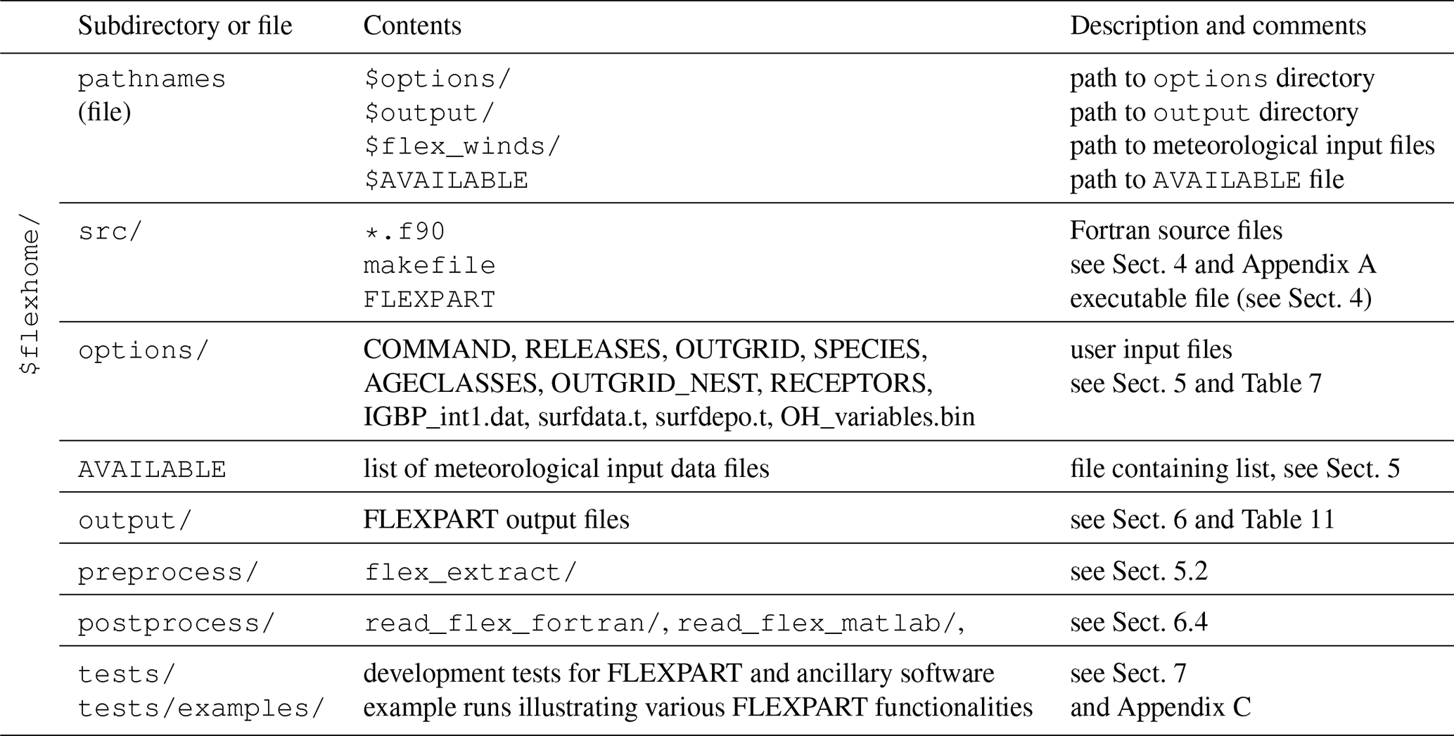
Despite the many changes and additions, in large part the operation of FLEXPART v10.4 still resembles the original version 1 design. Throughout this paper, we avoid repeating information on aspects of the model that have not changed since earlier model descriptions. The paper should therefore always be considered together with the publications of Stohl et al. (1998, 2005). To provide the necessary context for the rest of this paper, we provide a brief overview of the FLEXPART v10.4 directory structure in Table 1. The source code is contained in directory src. The pathnames of the input and output directories are stated in the file pathnames read by the FLEXPART executable. The directory options contains the parameters that define a run in files such as COMMAND (e.g., start and end times of the simulation, output frequency, etc.), RELEASES (definition of the particle releases), OUTGRID (output grid specifications) and others. All the output is written in a directory unique for each run. There are also other directories containing the model testing environment and example runs, as well as preprocessing and post-processing software (see Table 1).

Sensu stricto FLEXPART consists of the (Fortran) source files required to build an executable, not including external libraries such as those needed for input reading. The makefiles and the sample input as provided in the “options” may also be included under this term. However, in order to do real work with FLEXPART, one also needs to obtain meteorological input data (in the case of the ECMWF this is not trivial, so the flex_extract package is provided), and one needs to do post-processing. This is the reason why we include a selection of such tools here.

Table 1 Directory structure overview of the FLEXPART v10.4 software distribution. All listed directories are subdirectories of the installation root directory $flexhome/.

2 Updates of the model physics and chemistry

This section gives an overview of the main updates of the model physics and chemistry since the last published FLEXPART version, v6.2 (Stohl et al., 2005). Some developments have been published already separately, and in such cases we keep the description short, focusing on technical aspects of the implementation in FLEXPART that are important for model users or demonstrating applications not covered in the original papers.

2.1 Boundary layer turbulence

Subgrid-scale atmospheric motions unresolved by the meteorological input data need to be parameterized in FLEXPART. This is done by adding stochastic fluctuations based on Langevin equations for the particle velocity components (Stohl et al., 2005). In the ABL, the stochastic differential equations are formulated according to the well-mixed criteria proposed by Thomson (1987). Until FLEXPART version 9.2, the Eulerian probability density functions (PDFs) for the three velocity components were assumed to be three independent Gaussian PDFs. However, for the vertical velocity component, the Gaussian turbulence model is well suited only for stable and neutral conditions. In the convective ABL (CBL), turbulence is skewed since a larger area is occupied by downdrafts than by updrafts (e.g., Stull, 1988; Luhar and Britter, 1989). In such conditions, the Gaussian turbulence model is not appropriate for sources within the ABL, as it cannot reproduce the observed upward bending of plumes from near-ground sources or the rapid downward transport of plumes from elevated sources (Venkatram and Wyngaard, 1988). However, the Gaussian approximation has negligible influence once the tracer is mixed throughout the whole ABL.

Cassiani et al. (2015) developed an alternative Langevin equation model for the vertical particle velocity including both skewed turbulence and a vertical density gradient, which is now implemented in FLEXPART v10.4. This scheme can be activated by setting the switch CBL to 1 in the file COMMAND. In this case, the time step requirement for numerical stability is much more stringent than for the standard Gaussian turbulence model (typically, values of CTL=10 and IFINE=10 are required, also set in the file COMMAND). Therefore, also considering that the computation time required for each time step is about 2.5 times that of the standard Gaussian formulation, the CBL option is much more computationally demanding and not recommended for large-scale applications. However, for studies of tracer dispersion in the vicinity of individual point sources, the CBL option is essential to reproduce the characteristic features of CBL dispersion (Weil, 1985), while the additional computational burden remains tolerable.

Figure 1 shows a comparison between two simulations of dispersion from an elevated source, with the skewed and with the Gaussian turbulence model. It can be seen that the maximum time-averaged ground-level concentration is about 30 % higher for the skewed turbulence parameterization. This is the result of the plume centerline tilting downward to the surface in the vicinity of the source for the skewed turbulence case due to downdrafts being more frequent than updrafts. The plume also spreads faster in this case. These results are similar to those obtained by others (e.g., Luhar and Britter, 1989).

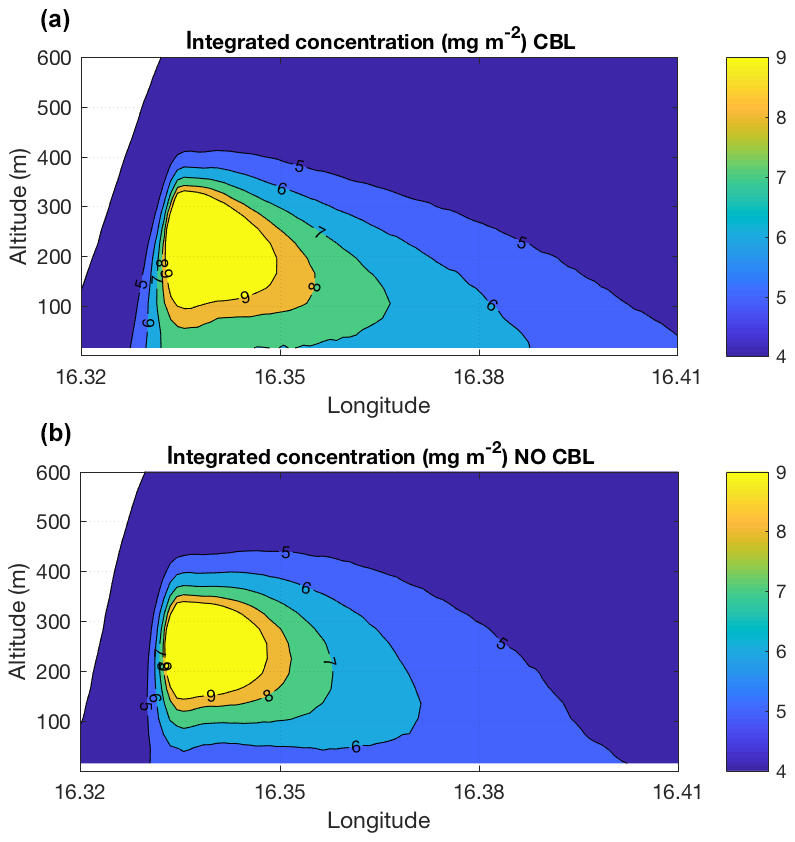
Figure 1 Comparison of FLEXPART results obtained with the skewed turbulence parameterization (a) and with the Gaussian turbulence parameterization (b). Shown are the tracer concentrations integrated over all latitudes as a function of altitude and longitude. The simulations used a point source emitting 100 kg of tracer per hour for a period starting on 1 July 2017 at 12:00 UTC and ending at 13:30 UTC. The source was located near Vienna (Austria) at 47.9157^∘ N and 16.3274^∘ E, 250 m above ground level. Results are averaged for the time period 12:40 to 13:00 UTC. Notice that the maximum ground-level concentration in panel (a) (ca. 7 mg m⁻²) is about 30 % higher than in panel (b) (5 mg m⁻²).

It is important to note that the CBL formulation smoothly transits to a standard Gaussian formulation when the stability changes towards neutral (Cassiani et al., 2015). However, the actual equation solved inside the model for the Gaussian condition is still different from the standard version as actual particle velocities rather than the scaled ones are advanced (see, e.g., Wilson et al., 1981; Rodean, 1996). Full details of the CBL implementation can be found in Cassiani et al. (2015).

To date, FLEXPART has mainly been used for large-scale applications. With this new CBL option, FLEXPART is now also well suited for the simulation of small-scale tracer dispersion or for the inverse modeling of point source emissions from near-field measurements – at least if the resolved winds are representative of the situation considered. In fact, to our knowledge FLEXPART is the only particle model considering both skewness in the vertical velocity distribution and vertical gradients in air density. Both these effects are particularly important in deep CBLs and can be additive with respect to simulated ground-level concentrations.

2.2 Turbulent diffusivity above the boundary layer

Above the atmospheric boundary layer, turbulent fluctuations can be represented with a turbulent diffusivity. The value of the diffusivity tensor controls the size and lifetimes of the filamentary structures caused by advection. Diffusivities are converted into velocity scales using ${\mathit{\sigma }}_{v_i}=\sqrt{\frac{\mathrm{2}{D}_i}{\mathrm{d}t}}$, where i is the direction. This corresponds to a mean diffusive displacement of ${\mathit{\sigma }}_{x_i}=\sqrt{\mathrm{2}{D}_i\mathrm{d}t}$, characteristic of Brownian motion. For i, only the vertical (v) and horizontal (h) directions are considered. The value of the vertical diffusivity D_z is related to the value of the horizontal diffusivity D_h by the square of the typical atmospheric aspect ratio for tracer structures κ≈100–250 (Haynes and Anglade, 1997).

FLEXPART uses by default a constant vertical diffusivity D_z=0.1 m² s⁻¹ in the stratosphere, following Legras et al. (2003), whereas a horizontal diffusivity D_h=50 m² s⁻¹ is used in the free troposphere. In general in the atmosphere, the values of the turbulent diffusivity depend on time and location, showing in particular seasonal, latitudinal and altitude variability: e.g., $D_{\mathrm{v}}={\mathrm{10}}^{-\mathrm{2}}$ m² s⁻¹ in the stratosphere (Balluch and Haynes, 1997) and D_h=10⁴ m² s⁻¹ (Pisso et al., 2009) in the troposphere. The values can be modified by the user in the COMMAND file (namelist variables d_trop and d_strat, in m² s⁻¹). As mentioned above, D_h≈κ²D_z, and therefore both values can be used interchangeably.

In FLEXPART version 6.2, the stratosphere and troposphere were distinguished based on a threshold of 2 pvu (potential vorticity units), with a maximal height of 18 km in the tropics and a minimal height of 5 km elsewhere. Such a threshold is well suited to midlatitudes, but it can differ from the thermal tropopause in the polar regions and close to the Equator. In FLEXPART 10.4, the thermal tropopause definition is used and is calculated using the lapse rate definition (Hoinka, 1997).

2.3 Gravitational settling

Gravitational settling of aerosols is implemented in FLEXPART as a process that changes the particle trajectories. The settling velocity is determined at each time step and added to the vertical wind velocity. In simulations in which a particle represents several species, all species are transported with the settling velocity of the first species. If this is not intended, simulations for the different species must be run separately. Gravitational settling velocities are also used in the calculation of dry deposition.

In older FLEXPART versions, gravitational settling was calculated using a single dynamic viscosity of air. With FLEXPART 8.2.1, the gravitational settling calculation was generalized to higher Reynolds numbers and it takes into account the temperature dependence of dynamic viscosity. This is done in subroutine get_settling.f90 in an iterative loop, wherein both the Reynolds number and the settling velocity are determined (Naeslund and Thaning, 1991). For initialization of the loop, Stokes' law and a constant viscosity estimate is used. The dynamic viscosity is calculated as a function of temperature using the formula of Sutherland (1893). A spherical shape of the particles is assumed in the settling calculation, which could be further extended in the future to allow for more complex particle shapes. For particle sizes of about 10 µm, settling velocities in the new FLEXPART version are not much different from earlier versions using the old settling calculation, typically less than 20 %. However, the differences are largest in the cold upper troposphere, implying, for instance, changes in the residence time of volcanic ash particles at heights relevant for aviation. The residence times in the upper troposphere are increased with the new scheme, but the effect is not particularly large, typically on the order of 20 %.

2.4 Wet deposition

In FLEXPART, the calculation of wet scavenging is divided into three parts. First, where scavenging occurs and which form it takes is determined (e.g., below- or within-cloud scavenging). Second, the scavenging coefficient is determined. Third, the actual removal of particle mass is calculated.

With respect to the first part, it is important to understand that wet scavenging occurs only in the presence of clouds and where precipitation occurs. In air columns without clouds, above the top of the clouds, and where neither the large-scale nor the convective precipitation rate exceeds 0.01 mm h⁻¹, no scavenging occurs. To quickly know where a particle is located relative to the clouds, in subroutines verttransform_ecmwf.f90 andverttransform_gfs.f90 each grid cell is categorized as being in a cloud-free column, above a cloud, inside a cloud or below a cloud. This cloud definition has been completely revised compared to earlier versions and is described in Sect. 2.4.1.

With respect to the second step, the scavenging coefficient Λ (s⁻¹) is determined in subroutine get_wetscav.f90. After a series of updates, in particular Grythe et al. (2017), FLEXPART now distinguishes between below-cloud and in-cloud scavenging and also has different parameterizations of Λ for gases and particles. For the latter, it also distinguishes between liquid-phase and ice-phase states. This yields in total six different parameterizations for Λ, described in Sect. 2.4.2 and 2.4.3.

In the third step, the removal of particle mass due to wet deposition is calculated. It takes the form of an exponential decay process (McMahon, 1979),

$$\begin{array}{}\text{(1)}& m(t+\mathrm{\Delta }t)=m\left(t\right)\exp (-\mathrm{\Lambda }\mathrm{\Delta }t),\end{array}$$

where m is the particle mass (kg) (it can also be a mass mixing ratio, depending on settings in file COMMAND). This removal of particle mass and corresponding accumulation of deposition at the surface is calculated in subroutine wetdepo.f90 and has not been changed since earlier versions.

2.4.1 Definition of clouds, cloud water content and precipitation

The location of clouds, the total cloud column water content and phase, and precipitation intensity and phase are needed in the calculation of the wet scavenging. Therefore, a three-dimensional cloud mask is defined in subroutine verttransform_ecmwf.f90 (or verttransform_gfs.f90 for GFS data). In previous FLEXPART versions, the cloud definition scheme was very simple and based on relative humidity (RH). In grid columns with precipitation, grid cells with RH >80 % were defined as in-cloud, and those with RH <80 % were set as below-cloud up to the bottom of the uppermost layer with RH >80 %. This was appropriate for the first version of FLEXPART, as the ECMWF had a similarly simple definition of clouds and more detailed information was not available from the ECMWF archives at the time.

If no cloud information is available from the meteorological data, the old RH-based scheme is still used in FLEXPART. However, nowadays, specific cloud liquid water content (CLWC; kg kg⁻¹) and specific cloud ice water content (CIWC; kg kg⁻¹) are available as 3-D fields in meteorological analyses from the ECMWF, and NCEP also provides the 3-D cloud water (liquid plus ice) mixing ratio (CLWMR; kg kg⁻¹), from here on referred to as q_c. A cloudy grid cell is defined when q_c>0. FLEXPART v10.4 can ingest the ECMWF CLWC and CIWC either separately or as a sum (q_c=CLWC+CIWC). However, to save storage space, we recommend retrieving only the sum, q_c, from the ECMWF, as the relative fractions of ice and liquid water can be parameterized quite accurately using Eq. (4).

The column cloud water (c_l; kg m⁻²), which is needed for the in-cloud scavenging parameterization, is calculated by integrating q_c over all vertical z levels:

$$\begin{array}{}\text{(2)}& c_{\mathrm{l}}=\sum _z{q}_{\mathrm{c}}\left(z\right){\mathit{\rho }}_{\mathrm{air}}\left(z\right)\mathrm{\Delta }z,\end{array}$$

where ρ_air(z) is the density of the air in the grid cell, and Δz is the vertical extent of the grid cell. In older FLEXPART versions, c_l was parameterized based on an empirical equation given in Hertel et al. (1995) using the subgrid (see below for a description of how subgrid is defined) surface precipitation rate I_s (mm h⁻¹). While such a parameterization is not needed anymore if q_c is available, it is still activated in the case that cloud water input data are missing. However, in order to ensure that c_l from the parameterization is statistically consistent with the cloud data, we derived the modified expression

$$\begin{array}{}\text{(3)}& c_{\mathrm{l}}=\mathrm{0.5}\times I_{\mathrm{s}}^{\mathrm{0.36}}\end{array}$$

using a regression analysis between existing cloud and precipitation data.

Precipitation is not uniform within a grid cell. To account for subgrid variability, it is assumed that precipitation is enhanced within a subgrid area and that no precipitation (and thus no scavenging) occurs outside this subgrid area. The subgrid area fraction and precipitation rate (I_s) are estimated from the grid-scale precipitation rate (I_t) based on values tabulated in Hertel et al. (1995). This parameterization of subgrid variability is used for all scavenging processes in FLEXPART and maintained from previous FLEXPART versions as described in Stohl et al. (2005).

The precipitation phase needed for the below-cloud scavenging scheme is simply based on ambient grid-scale temperature, with snow occurring below 0 ^∘C and rain above. For cloud water, c_l, we assume a temperature-dependent mixture of liquid and solid particles, for which the liquid fraction (α_L) is calculated based on the local temperature T,

$$\begin{array}{}\text{(4)}& {\mathit{\alpha }}_{\mathrm{L}}=({\displaystyle \frac{T-T_{\mathrm{I}}}{T_{\mathrm{L}}-T_{\mathrm{I}}}}{)}^{\mathrm{2}},\end{array}$$

where $T_{\mathrm{L}}={\mathrm{0}}^{\circ }$C and $T_{\mathrm{I}}=-\mathrm{20}$ ^∘C. For T>T_L, α_L=1 and for T<T_I, α_L=0. Even when CLWC and CIWC are available as separate fields, we derive the liquid fraction (α_L) of cloud water from the local temperature. The ice fraction α_I is 1−α_L. Comparisons have shown that CLWC is very accurately reproduced by α_Lq_c.

The cloud information should be linearly interpolated like the other variables, and situations in which the diagnosed cloud is incompatible with the precipitation rate (be it because of interpolation or because of convective precipitation accompanied by too shallow or lacking grid-scale clouds) need to receive special treatment. This is planned for a version upgrade in the near future in conjunction with a better interpolation scheme for precipitation (see Hittmeir et al., 2018). In certain cases, the deposition calculation of FLEXPART might be improved by using higher-resolution precipitation data from other sources such as from radar observations (Arnold et al., 2015); however, as the precipitation and ECMWF cloud data, and also the precipitation and wind fields, may not match, this does not guarantee better results.

2.4.2 Below-cloud scavenging

For gases, the scavenging coefficient, Λ, for below-cloud scavenging is calculated as described in Asman (1995),

$$\begin{array}{}\text{(5)}& \mathrm{\Lambda }=A{I}_{\mathrm{s}}^B,\end{array}$$

where the scavenging parameters A and B depend on the chemical properties of the gas and are specified in the SPECIES_nnn file as described in Sect. 5.1.3 (nnn represents the species number (0–999) used for the simulation). In older FLEXPART versions, this scheme was used also for aerosols; however, Grythe et al. (2017) developed a new aerosol scavenging scheme that is implemented in FLEXPART v10.4 and briefly summarized here.

The relevant processes of collision and attachment of ambient aerosol particles to falling precipitation depend mainly on the relationship between the aerosol and hydrometeor size and type (rain or snow) as well as to a lesser degree on the density and hygroscopicity of the aerosol. In FLEXPART v10.4, the dependence of scavenging on the sizes of both the aerosol and falling hydrometeors are taken into account by the schemes of Laakso et al. (2003) for rain and Kyrö et al. (2009) for snow. Both schemes follow the equation

$$\begin{array}{}\text{(6)}& \begin{array}{rl}{\log }_{\mathrm{10}}\left({\displaystyle \frac{\mathrm{\Lambda }}{{\mathrm{\Lambda }}_{\mathrm{0}}}}\right)=& C_{*}(a+b{D}_{\mathrm{p}}^{-\mathrm{4}}+c{D}_{\mathrm{p}}^{-\mathrm{3}}+d{D}_{\mathrm{p}}^{-\mathrm{2}}\\ & +e{D}_{\mathrm{p}}^{-\mathrm{1}}+f\left({\displaystyle \frac{I_{\mathrm{s}}}{I_{\mathrm{0}}}}{)}^{\mathrm{0.5}}\right),\end{array}\end{array}$$

where $D_{\mathrm{p}}={\log }_{\mathrm{10}}\frac{d_{\mathrm{p}}}{d_{\mathrm{p}\mathrm{0}}}$, d_p is the particle dry diameter provided in the SPECIES_nnn file, d_p0=1 m, Λ₀=1 s⁻¹ and I₀=1 mm h⁻¹. Coefficients for factors a–f are different for rain and snow scavenging and are given in Table 2. The C_* values are collection efficiencies that reflect the properties of the aerosol and must be given for both rain ($C_{*}=C_{\text{rain}}$) and snow scavenging ($C_{*}=C_{\text{snow}}$) in the SPECIES_nnn file. Notice that by setting C_snow=0, below-cloud scavenging by snowfall is switched off (similarly, C_rain=0 for rain).

Laakso et al. (2003)Kyrö et al. (2009)

Table 2 Parameters used in Eq. (6) for below-cloud scavenging.

2.4.3 In-cloud scavenging

For in-cloud scavenging of both aerosols and gases, Λ is calculated as described in Grythe et al. (2017):

$$\begin{array}{}\text{(7)}& \mathrm{\Lambda }=i_{{\mathrm{c}}_{\mathrm{r}}}{S}_i{I}_{\mathrm{s}},\end{array}$$

where $i_{{\mathrm{c}}_{\mathrm{r}}}=\mathrm{6.2}$ is the cloud water replenishment factor, which was determined empirically in Grythe et al. (2017) (there it was named ic_r), and S_i is proportional to the in-cloud scavenging ratio, which is derived differently for gases and aerosols.

For gases, $S_i=\frac{\mathrm{1}}{\frac{\mathrm{1}-c_{\mathrm{l}}}{HRT}+c_{\mathrm{l}}}$, where H is Henry's constant (describing the solubility of the gas and specified in the SPECIES_nnn file), R is the gas constant and T is temperature. Notice that this is applied for both liquid-phase and ice clouds.

For aerosols, the in-cloud scavenging is dominated by activated particles forming cloud droplets or ice nuclei. Those may eventually combine to form a hydrometeor that falls out of the cloud, thus removing all aerosol particles contained in it. Therefore, S_i depends on the nucleation efficiency (F_nuc) and c_l:

$$\begin{array}{}\text{(8)}& S_i={\displaystyle \frac{F_{\text{nuc}}}{c_{\mathrm{l}}}}.\end{array}$$

F_nuc describes how efficiently the aerosol particles are activated as cloud droplet condensation nuclei (CCN) or ice nuclei (IN):

$$\begin{array}{}\text{(9)}& F_{\text{nuc}}={\mathit{\alpha }}_{\mathrm{L}}{\mathrm{CCN}}_{\text{eff}}+{\mathit{\alpha }}_{\mathrm{I}}{\mathrm{IN}}_{\text{eff}},\end{array}$$

where the relative abundances of the liquid and ice phase are accounted for by the factor α_L. Values for the efficiencies, CCN_eff and IN_eff, are available from the literature for many different types of aerosols (e.g., black carbon, mineral dust particles or soluble particles) and some have been collected in SPECIES_nnn files distributed with FLEXPART (see Sect. 5.1.3). The CCN_eff and IN_eff values are set for an aerodynamic particle radius of 1 µm, but CCN and IN efficiencies increase with increasing particle size. The in-cloud parameterization takes this into account. For further details on the wet scavenging scheme used in FLEXPART, see Grythe et al. (2017).

2.4.4 Influence of wet scavenging on the aerosol lifetime

Aerosol wet scavenging controls the lifetime of most aerosols. In Fig. 2, we compare modeled e-folding lifetimes from a number of FLEXPART simulations using different model versions and switching off in-cloud and below-cloud scavenging in FLEXPART v10.4 with measured lifetimes. The parameter settings in FLEXPART used for these comparisons were the same as used by Grythe et al. (2017). To derive aerosol lifetimes in a consistent way from both measurements and model simulations, a radionuclide attached to ambient aerosol and a noble gas radionuclide were used. Kristiansen et al. (2016) used the same method to compare many different aerosol models, and we refer to their paper for more details on the method. For our model simulations, several size bins of aerosols were used, though total concentrations and lifetimes are largely controlled by 0.4 and 0.6 µm particles (see Grythe et al., 2017). E-folding lifetimes increase from 5.8 to 10.0 d between FLEXPART v9 and v10.4. A simulation performed with v10.4 but which emulated the in-cloud scavenging of v9 showed that the difference is mainly due to the decreased in-cloud scavenging in the new removal scheme compared to the old one. Notice that the lifetime obtained with v10.4 is much closer to the observation-based lifetimes. Turning off the below-cloud removal has a relatively small effect, increasing the lifetime to 11 d, whereas turning off the in-cloud removal extends the lifetime to the unrealistic value of 66 d (see bottom two panels in Fig. 2). This highlights the dominant role of in-cloud removal for accumulation-mode particles in FLEXPART.

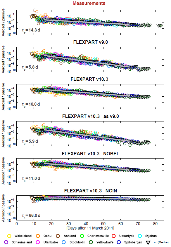
Figure 2 Aerosol lifetimes estimated from the decrease in radionuclide ratios (aerosol-bound ¹³⁷Cs and noble gas ¹³³Xe as a passive tracer) with time after the Fukushima nuclear accident, as measured and modeled at a number of global measurement stations. For details on the method, see Kristiansen et al. (2016). E-folding lifetimes, τ_e, are estimated based on fits to the data and reported in each panel. In the top panel, the observed values are shown and in subsequent panels from the top, modeled values are given for FLEXPART v9, FLEXPART v10.4, FLEXPART v10.4 with parameter settings to emulate removal as in v9, FLEXPART v10.4 with no below-cloud removal and FLEXPART v10.4 with no in-cloud removal.

Notice that compared to older versions of FLEXPART, the SPECIES_nnn files now include additional parameters related to the wet deposition scheme. Old input files, therefore, need to be updated for use with FLEXPART v10.4. The required format changes are detailed in Sect. 5.1.3.

2.5 Source–receptor matrix calculation of deposited mass backward in time

When running FLEXPART forward in time for a depositing species with a given emission flux (kilograms per release as specified in file RELEASES), the accumulated wet and dry deposition fluxes (ng m⁻²) are appended to the FLEXPART output files (grid_conc_date and/or grid_pptv_date, for which date represents the date and time in format YYYYMMDDhhmmss; see Sect. 6) containing the atmospheric concentration and/or volume mixing ratio output. The deposition is always given in mass units, even if atmospheric values are given in mixing ratio units. In contrast to concentration values, deposition quantities are accumulated over the time of the simulation, so the deposited quantities generally increase during a simulation (except when radioactive decay is activated, which also affects deposited quantities and can decrease them).

As discussed in Sect. 1, running FLEXPART backward in time for calculating SRRs is more efficient than running it forward if the number of (potential) sources is larger than the number of receptors. For atmospheric concentrations (or mixing ratios), the backward mode has been available from the very beginning and in an improved form since FLEXPART v5 (Stohl et al., 2003; Seibert and Frank, 2004). This has proven very useful for the interpretation of ground-based, shipborne or airborne observations (e.g., to characterize sources contributing to pollution plumes). Furthermore, the inversion scheme FLEXINVERT (Thompson and Stohl, 2014) that is used to determine the fluxes of greenhouse gases is based on backward simulations. However, there are also measurements of deposition on the ground, e.g., in precipitation samples or ice cores, and for this type of measurement no backward simulations were possible until recently. Therefore, Eckhardt et al. (2017) introduced the option to calculate SRR values in backward mode also for wet and dry deposition, and a first application to ice core data was presented by McConnell et al. (2018). It is anticipated that quantitative interpretation of ice core data will be a major application of the new backward mode, which is efficient enough to allow for the calculation of, for example, 100 years of seasonally resolved deposition data in less than 24 h of computation time.

We illustrate the different backward modes and explain the required settings with an example. The calculations were run for a single receptor location, Ny-Ålesund in Spitsbergen (78.93^∘ N, 11.92^∘ E) and for the 24 h period from 18 August 2013 at 20:00 UTC to 19 August 2013 at 20:00 UTC. SRR values are calculated for the atmospheric concentration averaged over the layer 0–100 m a.g.l., as well as for wet and dry deposition. The substance transported is black carbon (BC), which is subject to both dry and wet deposition. Backward simulations for wet and dry deposition must always be run separately. In order to obtain SRR values for total deposition, results for wet and dry deposition need to be summed.

The backward mode is activated by setting the simulation direction, LDIRECT in file COMMAND (see Sect. 5), to −1. The three simulations are obtained by consecutively setting IND_RECEPTOR to 1 (for concentration), 3 (wet deposition) and 4 (dry deposition). IND_SOURCE is always set to 1, meaning that the sensitivities (SRR values) are calculated with respect to physical emissions in mass units. A complete list of possible options is reported in Table 1 of Eckhardt et al. (2017).

Figure 3 shows the resulting SRR (i.e., emission sensitivity) fields for the concentration as well as dry and wet deposition at the receptor. Dry deposition occurs on the Earth's surface, and therefore particles are released in a shallow layer adjacent to the surface. Its height is consistent with the shallow depth over which dry deposition is calculated in forward mode (user settings for the release height are ignored for dry deposition backward calculations). Dry deposition rates are the product of the surface concentration and the deposition velocity. Therefore, the SRR fields for surface concentration (Fig. 3a) and dry deposition (Fig. 3b) show similar patterns, in this case indicating high sensitivity for sources over Scandinavia and northwestern Russia. The differences in the spatial patterns are mainly due to temporal variability in the dry deposition velocity at the receptor caused by varying meteorological conditions (e.g., stability) and surface conditions during the 24 h release interval.

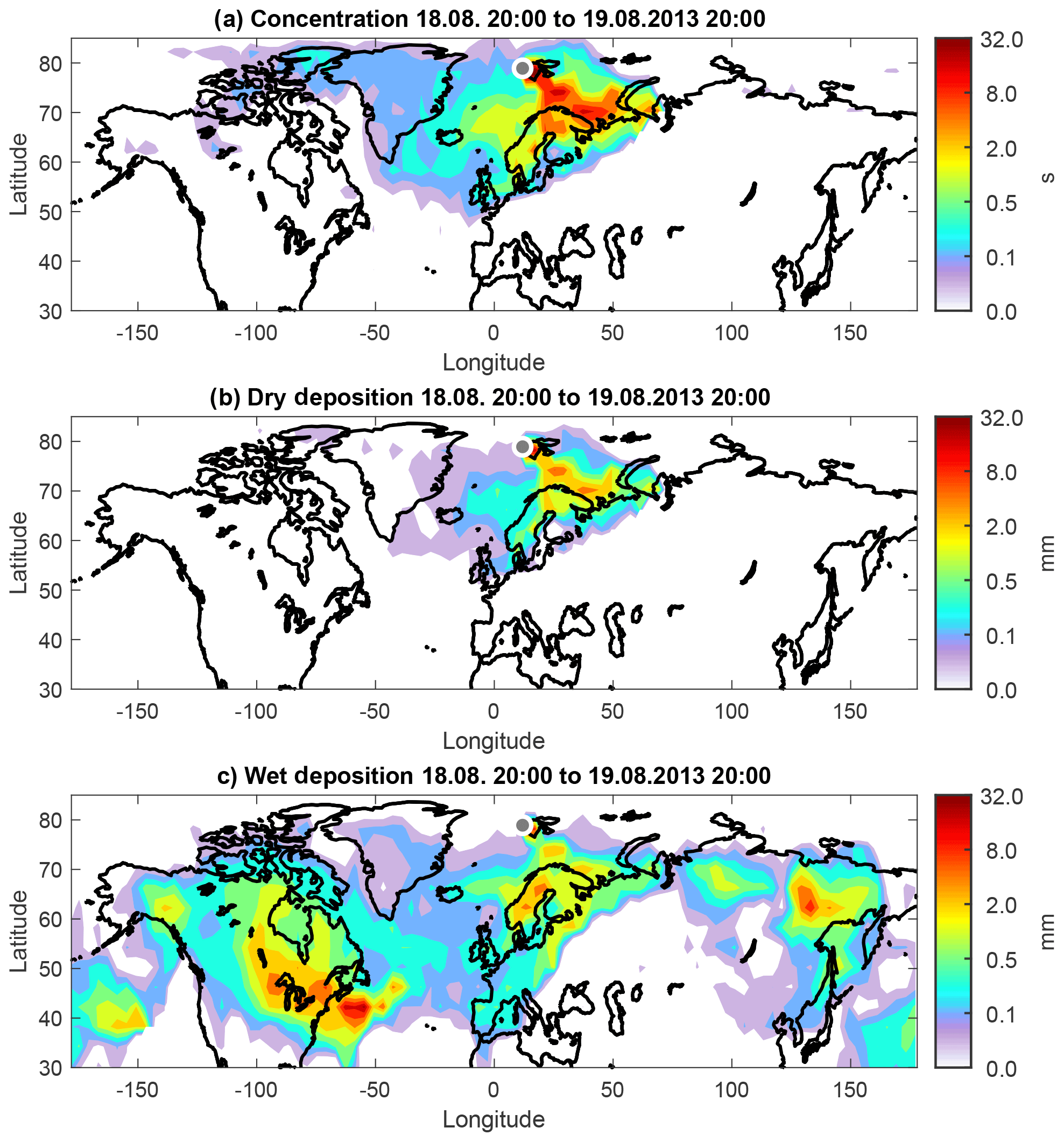
Figure 3 Source–receptor relationships (for emissions occurring in the lowest 100 m a.g.l.) for black carbon observed at Ny-Ålesund in Svalbard for a 24 h period starting on 18 August 2013 at 20:00 UTC. The sensitivities were calculated for (a) concentrations (s) in the layer 0–100 m a.g.l., (b) dry deposition (mm) and (c) wet deposition (mm).

Wet deposition, on the other hand, can occur anywhere in the atmospheric column from the surface to the top of the precipitating cloud. FLEXPART automatically releases particles in the whole atmospheric column (again, user settings for the release height are ignored), but particles for which no scavenging occurs (e.g., those above the cloud top or when no precipitation occurs) are immediately terminated. Therefore, and because of the vertical variability of the scavenging process, the sensitivity for the deposited mass can deviate significantly from the sensitivity corresponding to surface concentration. Here (Fig. 3c), the sensitivity is high over Scandinavia and northwestern Russia, as was already seen for surface air concentrations and dry deposition. However, in addition, sources located in North America and eastern Siberia also contribute strongly to wet deposition. The maximum over the ocean close to the North American east coast is likely due to lifting in a warm conveyor belt, followed by fast transport at high altitude.

Concentration, dry deposition and wet deposition at the receptor can be calculated from the SRR fields shown in Fig. 3 as follows.

$$\begin{array}{}\text{(10)}& \begin{array}{rl}c& ={\mathit{m}}_{\mathrm{c}}\cdot \mathit{q}\\ d_{\mathrm{d}}& ={\mathit{m}}_{\mathrm{d}}\cdot \mathit{q}\\ d_{\mathrm{w}}& ={\mathit{m}}_{\mathrm{w}}\cdot \mathit{q}\end{array}\end{array}$$

Here, c is the modeled concentration (in kg m⁻³), d_d the dry deposition rate and d_w the wet deposition rate (both in kg m⁻² s⁻¹). In this specific case with only a single scalar receptor, the source–receptor matrix degenerates to a vector of the SRR values, one for each of the three types of receptor (m_c for concentration in units of seconds, m_d for dry deposition and m_w for wet deposition, both in units of meters). In order to obtain the concentration or the deposition rates, these vectors need to be multiplied with the vector of emissions q (kg m⁻³ s⁻¹). If the total deposition is desired, the deposition rates d_d and d_w can be multiplied with the receptor time interval ΔT_r, in our case 86 400 s (24 h). Note that this is the period during which particles are released according to the specification of the RELEASES file. The emission fluxes must be volume averages over the output grid cells specified in the OUTGRID file, typically surface emission fluxes (in kg m⁻² s⁻¹) divided by the height of the lowermost model layer.

2.6 Sensitivity to initial conditions

Backward simulations with FLEXPART in the context of inverse modeling problems typically track particles for several days up to a few weeks. This is sufficient to estimate concentrations at the receptor only for species with atmospheric lifetimes shorter than this period. Many important species (e.g., greenhouse gases such as methane) have considerably longer lifetimes. For such long-lived species, most of the atmospheric concentration variability is still caused by emission and loss processes occurring within the last few days before a measurement because the impact of processes occurring at earlier times is smoothed out by atmospheric mixing. This leads to a relatively smooth “background” (in time series analyses sometimes also called a baseline) that is often a dominant fraction of the total concentration but that does not vary much with time, with short-term fluctuations on top of it. The signal of the regional emissions around the measurement site is mostly contained in the short-term concentration fluctuations but in order to use it in inverse modeling, the background still needs to be accounted for, as otherwise no direct comparison to measurements is possible.

One simple method is to estimate the background from the measurements as, e.g., in Stohl et al. (2009). A better approach is to use a concentration field taken from a long-term forward simulation with an Eulerian model or with FLEXPART itself, especially if nudged to observations (Groot Zwaaftink et al., 2018), as an initial condition for the backward simulation. This field needs to be interfaced with the FLEXPART backward simulation by calculating the receptor sensitivity to the initial conditions (see Eqs. 2–6 in Seibert and Frank, 2004). For instance, for a 10 d backward simulation, the concentration field needs to be sampled at those points in time and space when and where each particle trajectory terminates 10 d back in time. Furthermore, it is necessary to quantify the effects of deposition or chemical loss during the backward simulation on this background (the factor p(0) in Seibert and Frank, 2004). For example, chemical reactions with hydroxyl radicals will reduce initial concentrations of methane en route to the receptor, even though this is not much during a 10 d period.

Since version 8.2, FLEXPART has provided an option to quantify the influence of initial conditions on the receptor in backward simulations, which is activated with the switch LINIT_COND in file COMMAND. Then, gridded fields containing the sensitivities to background mixing ratios (or concentrations, depending on user settings for the switch LINIT_COND in file COMMAND) are produced and stored in the output files grid_initial_nnn (nnn stands for the species number) on the same 3-D grid as the regular output, defined in the files OUTGRID and OUTGRID_NEST. In this case, a concentration would be calculated as

$$\begin{array}{}\text{(11)}& c={\mathit{m}}_{\mathrm{i}}\cdot {\mathit{c}}_{\mathrm{b}}+{\mathit{m}}_{\mathrm{c}}\cdot \mathit{q},\end{array}$$

where m_i denotes the sensitivity to the initial condition and c_b the background concentration when and where particles are terminated.

Figure 4 shows an example of the use of the sensitivities of receptor mixing ratios (here, of methane) to both surface emissions and initial conditions. The panel (b) shows the sensitivity to surface emissions on one particular day, and the panels (c) and (d) show the sensitivity to initial conditions below and above 3000 m for the same day. Both results are from an 8 d backward simulation from one receptor site in Sweden. It can be seen that the sensitivity to emissions is highest close to the station, but there is also substantial sensitivity to emission uptake over large parts of central and eastern Europe. The particles terminated 8 d before arrival at the receptor in a roughly croissant-shaped area covering large parts of Europe and the North Atlantic, as indicated by the sensitivity to initial conditions. Most of the sensitivity is located below 3000 m but there is also some influence from higher levels. Notice that only two layers are shown in Fig. 4, whereas the real model output has much higher vertical resolution.

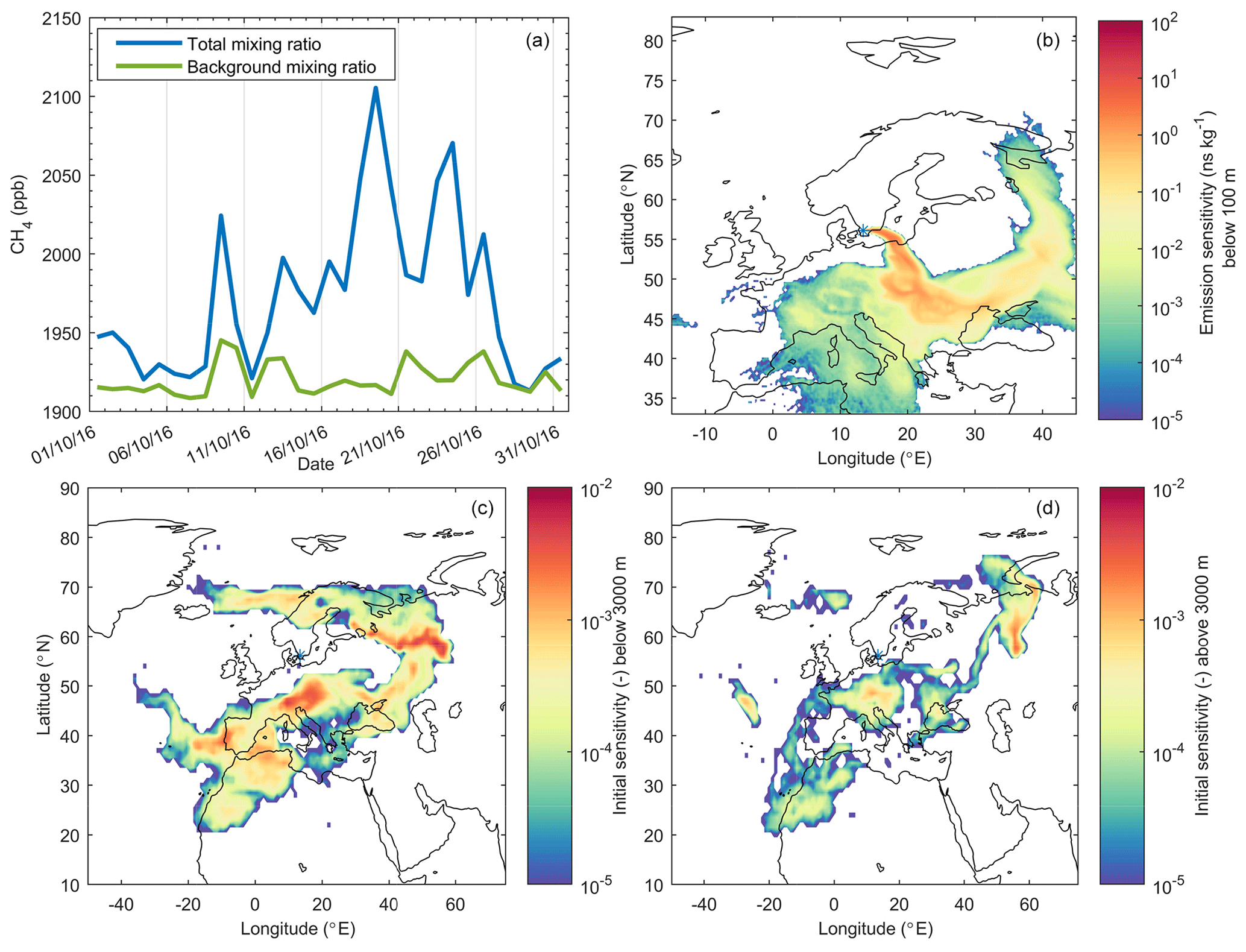
Figure 4 Example of FLEXPART 8 d backward runs for methane from a site in southern Sweden (Hyltemossa) demonstrating the combined use of sensitivities to emissions and initial conditions. (a) Time series of methane background mixing ratios and total mixing ratios in October 2016. (b) Sensitivity of the methane mixing ratio at Hyltemossa on 19 October 2016 to methane emissions at the surface. (c) Sensitivity of the methane mixing ratio at Hyltemossa on 19 October 2016 to methane initial conditions below 3000 m. (d) Sensitivity of the methane mixing ratio at Hyltemossa on 19 October 2016 to methane initial conditions above 3000 m. Blue asterisks on the maps mark the receptor location.

The sensitivity to initial conditions was interfaced with a domain-filling methane forward simulation as described in Groot Zwaaftink et al. (2018) (not shown), while the emission sensitivity was interfaced with an emission inventory for methane (not shown), as given by Eq. (11). This was done for daily simulations throughout 1 month, thus generating a time series of background mixing ratios (from the first term in Eq. 11 only) and total mixing ratios (Fig. 4a). The latter include the contributions from emissions during the 8 d backward simulation. It can be seen that the methane background advected from 8 d back varies relatively little between about 1910 and 1940 ppbv, while the emission contributions vary from 0 (on 29 October) to about 200 ppbv (on 19 October, the date for which the sensitivity plots are shown).

In practical applications for inverse modeling, source–receptor sensitivities are often only needed at the surface (as most emissions occur there), while sensitivities to the background are needed in 3-D. By setting the option SURF_ONLY to 1 in the COMMAND file, the regular output files grid_time_date_nnn containing the source–receptor sensitivities will include only the first vertical level as defined in the file OUTGRID, while the full vertical resolution is retained in grid_initial_nnn files containing the sensitivities to the initial conditions. Since the data amounts stored in the grid_time_date_nnn files can be much larger than in the grid_initial_nnn files, this is a highly efficient way to save storage space. This setup also interfaces directly with the inverse modeling package FLEXINVERT (Thompson and Stohl, 2014). An application can be found in Thompson et al. (2017) wherein initial conditions were taken from a gridded observation product. A further output option, which was also introduced for practical considerations of inverse modeling, is the LINVERSIONOUT option in the file COMMAND. If LINVERSIONOUT is set to 1, then the grid_time_date_nnn and grid_initial_nnn files are written per release with a time dimension of footprints instead of the default per footprint with a time dimension of releases. Since inverse modeling assimilates atmospheric observations and each observation is represented by a single release, it is computationally more efficient to read in the grid files separated by release. This output format also interfaces directly with FLEXINVERT.

2.7 Chemical reactions with the hydroxyl radical (OH)

The hydroxyl (OH) radical reacts with many gases and is the main cleansing agent in the atmosphere. While it is involved in highly nonlinear atmospheric chemistry, for many substances (e.g., methane) a simplified linear treatment of loss by OH is possible using prescribed OH fields. For this, monthly averaged ${\mathrm{3}}^{\circ }\times \mathrm{5}{}^{\circ }$ resolution OH fields for 17 atmospheric layers are used in FLEXPART. The fields were obtained from simulations with the GEOS-Chem model (Bey et al., 2001) and are read from the file OH_variables.bin by the subroutine readOHfield.f90.

Tracer mass is lost by reaction with OH if a positive value for the OH reaction rate is given in the file SPECIES_nnn. In FLEXPART v10.4, the OH reaction scheme was modified to account for (i) hourly variations in OH and (ii) the temperature dependence of the OH reaction rate (Thompson et al., 2015). This makes the chemical loss calculations more accurate, especially for substances with shorter lifetimes (of the order of weeks to months), for example ethane. Hourly OH fields are calculated from the stored monthly fields by correcting them with the photolysis rate of ozone calculated with a simple parameterization for cloud-free conditions based on the solar zenith angle (gethourlyOH.f90):

$$\begin{array}{}\text{(12)}& \text{OH}={\displaystyle \frac{j}{j^{*}}}{\text{OH}}^{*},\end{array}$$

where j represents the hourly photolysis rates calculated for all 3-D locations in the field, while j^* represents the corresponding monthly mean rates, precalculated and stored in file OH_variables.bin together with the monthly mean fields OH^* (see Sect. 5.1.8). The motivation for this is that OH production closely follows the production of O(¹D) by the photolysis of ozone, allowing for this simple parameterization of OH variability. At any time, two hourly OH fields are in memory and are interpolated to the current time step. Figure 5 shows the annual and daily variation of OH for two locations as obtained with this simple parameterization.

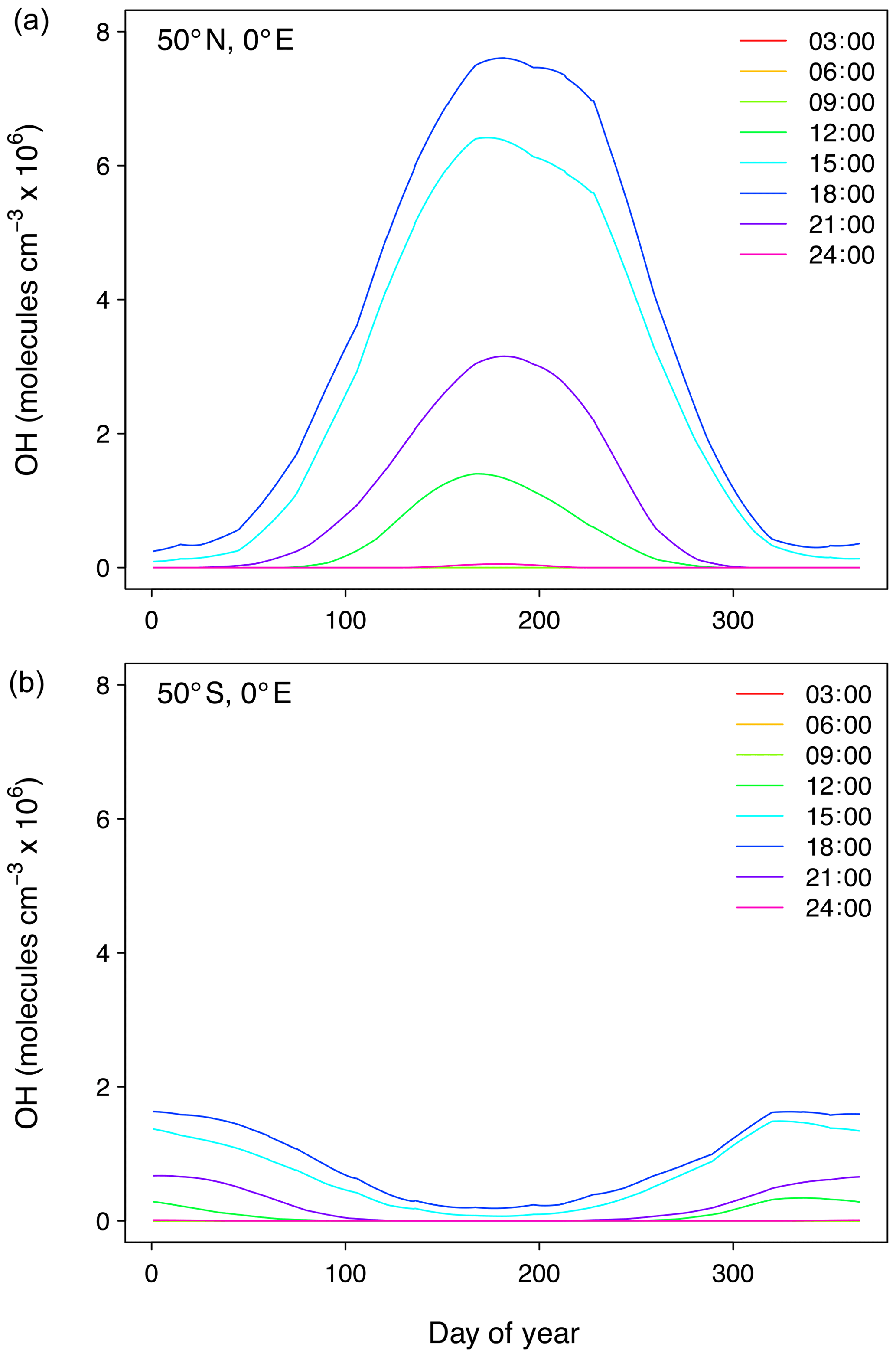
Figure 5 Annual and daily OH concentration variation as obtained with the simple parameterization based on photolysis rates of ozone for two locations, one in the Northern Hemisphere (a) and one in the Southern Hemisphere (b). Line labels correspond to the time of day.

The OH reaction rate κ (s⁻¹) is calculated in ohreaction.f90 using the temperature-dependent formulation

$$\begin{array}{}\text{(13)}& \mathit{\kappa }=C{T}^N{e}^{-D/T}\left[\mathrm{OH}\right],\end{array}$$

where C, N and D are species-specific constants (assigned in the SPECIES_nnn files), T is the absolute temperature, and [OH] the OH concentration (Atkinson, 1997). As the OH concentration in file OH_variables.bin is given in units of molecules per cubic centimeter, the unit of C needs to be in cubic centimeters per molecule per second (cm³ molecule⁻¹ s⁻¹). The mass m of a given species after reaction with OH is determined as

$$\begin{array}{}\text{(14)}& m(t+\mathrm{\Delta }{t}^{\prime })=m\left(t\right)e^{-\mathit{\kappa }\mathrm{\Delta }{t}^{\prime }},\end{array}$$

where Δt^′ is the reaction time step (given by lsynctime).

Backwards compatibility with the former temperature-independent specification of the OH reaction (version 9 and before) can be achieved by setting the constant N in the SPECIES_nnn file to zero. The constants C and D can be derived from the former parameters as follows:

$$\begin{array}{}\text{(15)}& C={\mathit{\kappa }}_{\mathrm{r}}{e}^{D/T_{\mathrm{r}}}\end{array}$$

and

$$\begin{array}{}\text{(16)}& D=A/\mathrm{R},\end{array}$$

where A is the activation energy, R is the gas constant and κ_r is the former OH reaction rate (referring to T_r=298 K), which were specified in the SPECIES_nnn file for earlier versions.

OH fields other than those provided with the model code have been tested in FLEXPART. These fields may have higher spatial and temporal resolution (e.g., Fang et al., 2016), which is important for chemical species with short lifetimes. Users are required to modify readOHfield.f90 and gethourlyOH.f90 to read in other OH fields and be aware that expressions of the OH reaction rate or reaction with OH might differ from those in the above equations. If this is the case users need to modify ohreaction.f90, too.

2.8 Dust mobilization scheme

Desert dust is a key natural aerosol with relevance for both climate and air quality. FLEXPART has been used earlier with preprocessors to initialize dust amounts from wind speed and surface properties following Tegen and Fung (1994) (Sodemann et al., 2015). Now a dust mobilization routine has been included as a preprocessing tool in FLEXPART v10.4. The scheme, called FLEXDUST, was developed to simulate mineral dust transport with FLEXPART in forward or backward simulations (Groot Zwaaftink et al., 2016). This module runs independently from FLEXPART and produces gridded output of mineral dust emissions as well as input files (RELEASES) that can be used for FLEXPART simulations of atmospheric transport. It can thus be considered a preprocessing (for forward simulations) or post-processing tool (for backward simulations) for FLEXPART v10.4.

In FLEXDUST, emission rates are estimated according to the emission scheme proposed by Marticorena and Bergametti (1995). We thereby assume that sandblasting occurs in the case that sand is present and a minimum threshold based on the size-dependent threshold friction velocity following Shao and Lu (2000) can be applied. The following are used as input for the model: ECMWF operational analysis or ERA-Interim reanalysis data, Global Land Cover by National Mapping Organizations version 2 (Tateishi et al., 2014), and and sand and clay fractions from the Global Soil Data Task (2014). Erodibility is enhanced in topographic depressions, and dust emissions are modified by soil moisture and snow cover. The module includes high-latitude dust sources in the Northern Hemisphere. These sources are rarely included in global dust models, even though they appear important for the climate system and substantially contribute to dust in the Arctic (Bullard et al., 2016; Groot Zwaaftink et al., 2016). Icelandic deserts in particular are known to be highly active, and a high-resolution surface type map for Iceland can therefore be included in FLEXDUST simulations (Arnalds et al., 2016; Groot Zwaaftink et al., 2017). Like in FLEXPART, nested meteorological fields can be used for specific regions of interest. The size distribution of emitted dust follows Kok (2011), is independent of friction velocity and is by default represented by 10 size bins. This can be changed depending on known properties or assumptions of dust sources. The dust particles are assumed to be spherical in FLEXPART. An example of annual mean dust emissions from 1990 to 2012 calculated with FLEXDUST driven with ERA-Interim meteorology is shown in Fig. 6. Further details on FLEXDUST, including model evaluation, are given by Groot Zwaaftink et al. (2016). The source code is available from the git repository: https://git.nilu.no/christine/flexdust.git (last access: 30 October 2019).

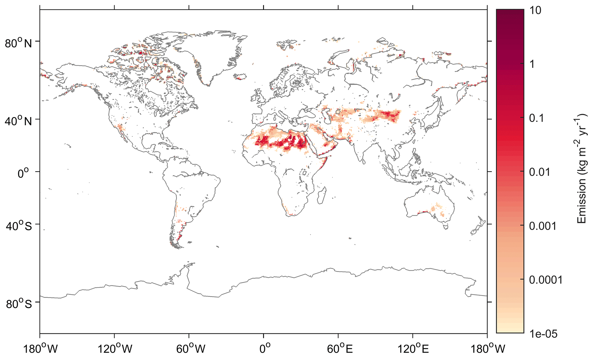
Figure 6 Average annual dust emission for the period 1990–2012 estimated with FLEXDUST driven with ERA-Interim meteorology.

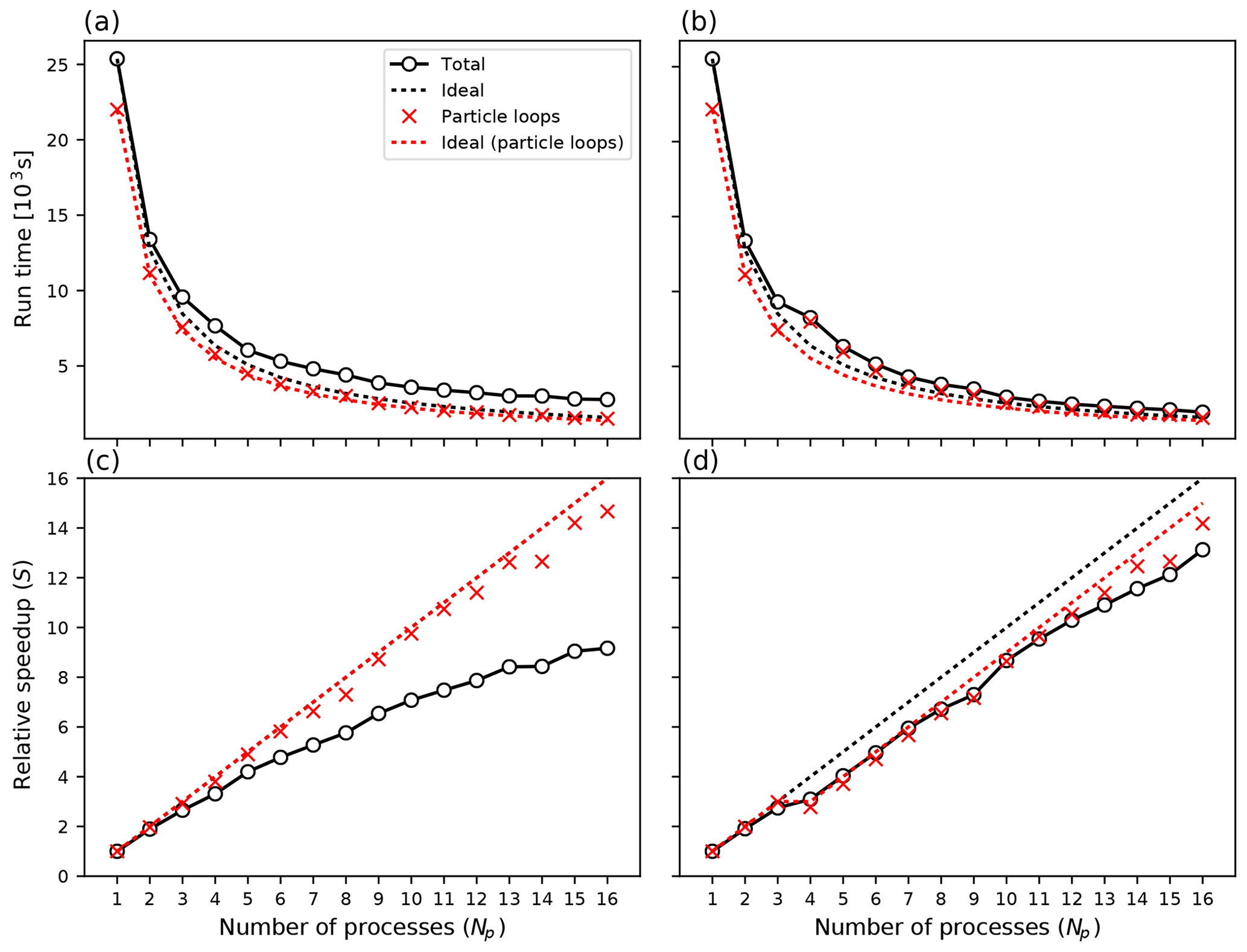
Figure 7 Computational time (a, b) and speedup (c, d) for up to 16 processes on a single node. In panels (a, c), all processes read meteorological input data, whereas in panels (b, d), a dedicated process reads and distributes input data for N_p≥4.

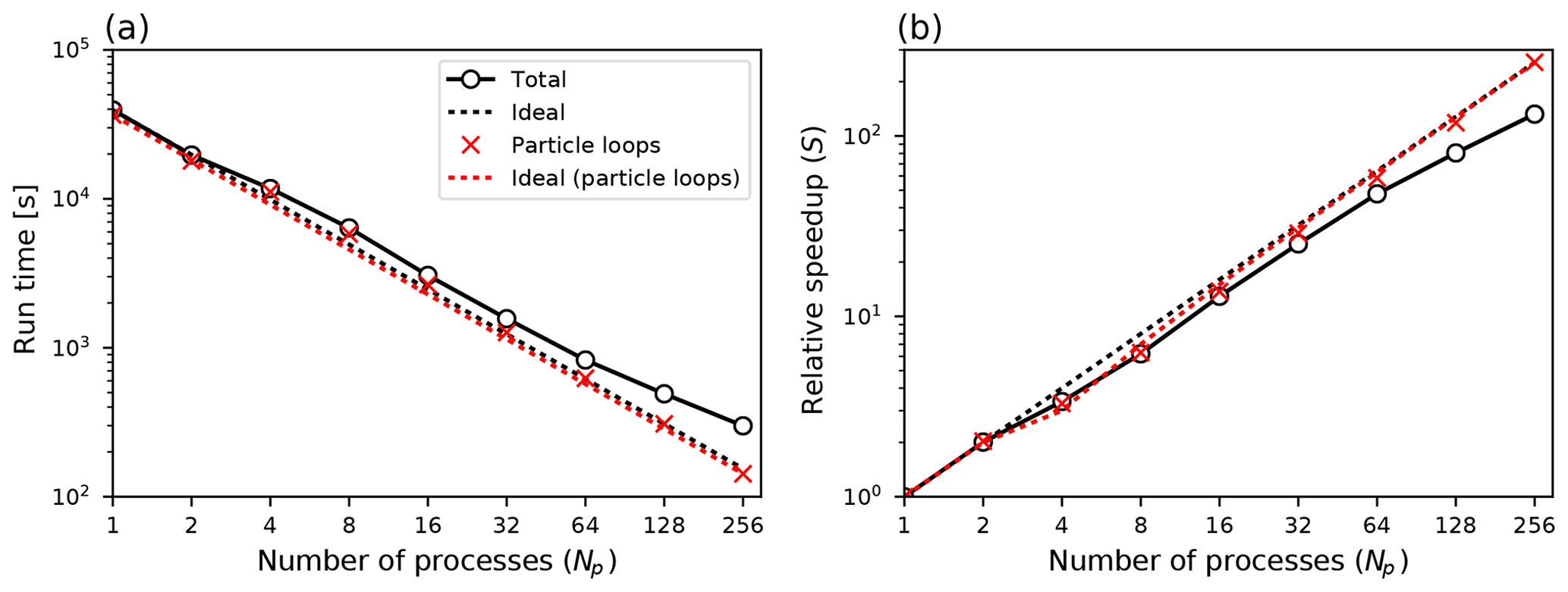
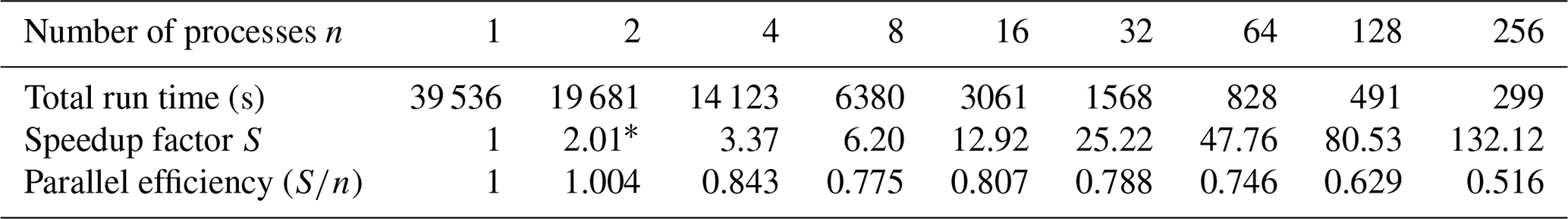
Figure 8 Computational time (a) and speedup (b) for up to 256 processes on 16 nodes. Logarithmic scaling along both axes. For n≥4 a dedicated process reads and distributes input data.

3 Parallelization

In a Lagrangian model like FLEXPART, particles move totally independently of each other. This facilitates efficient parallelization of the code. The most simple and often most effective way is running several instances of the model in parallel. For example, if the model is to be run backwards (for 10 d, for example) at regular intervals from a measurement site for a year, one could run the model separately, in parallel, for monthly subperiods. The total computation time of the 12 monthly processes together is nearly the same as if the model is run as one process for the whole year. Some overhead in processing input data occurs because, in the above example, 10 extra days of data per process are needed to calculate trajectories 10 d back into the preceding month. One disadvantage of that approach is that the memory needed for holding the meteorological input data and the model output fields is multiplied. However, this overhead is often small; thus, this approach has been used very often by FLEXPART users in the past.

Even if a task cannot easily be decomposed into runs for different periods or sources, trivial parallelization is still possible if a large number of particles is desired, for example in a domain-filling simulation for which tens of millions of particles may be used. The strategy in this case would be to assign a fraction of the particles to each run. Note that different random seeds should be used for each run, which requires a manual change and recompilation of the code.

As a user-friendly alternative, FLEXPART v10.4 has been parallelized using standard parallelization libraries. Common parallelization libraries are Open Multi-Processing (OpenMP; http://www.openmp.org/, last access: 30 October 2019), which is designed for multicore processors with shared memory, and Message Passing Interface (MPI, 2015) for distributed memory environments. Examples of other Lagrangian particle models that have been parallelized are NAME (Jones et al., 2007) and FLEXPART–WRF (Brioude et al., 2013), which use a hybrid approach (OpenMP+MPI). For FLEXPART v10.3 we decided to use a pure MPI approach for the following reasons.

• It is simpler to program than a hybrid model and more flexible than a pure OpenMP model.

• While OpenMP in principle may be more effective in a shared memory environment, MPI can often perform equally well or better provided there is not excessive communication between the processes.

• MPI offers good scalability and potentially low overhead when running with many processes.

3.1 Implementation

The FLEXPART code contains several computational loops over all the particles in the simulation, which is where most of the computational time is spent for simulations with many particles. The basic concept behind our parallel code closely resembles the “trivial parallelization” concept described above. When launched with a number of processes, N_p, each process will separately calculate how many particles to release per location, attempting to achieve an approximately even distribution of particles among the processes while keeping the total number of particles the same as for a simulation with the serial version. Each running process will generate an independent series of random numbers and separately calculate trajectories and output data for its set of particles. Explicit communications between processes are only used when the output fields are combined at the master process (MPI rank 0) using MPI_Reduce operations, before writing the output. Also, in the case in which the output of all individual particle properties is desired (option IPOUT1 = 1 or 2 in file COMMAND), we let each process append its data to the same file. We thus avoid the costly operation of transferring particle properties between processes. The performance of the implementation is discussed in Sect. 3.2 (see Fig. 7).

Some parts of the code are not simply loops over particles, most notably the routines for reading and transforming the input meteorological data. It follows that the performance gain of using parallel FLEXPART in general is better for simulations with a larger number of particles. We have, however, implemented a feature whereby instead of having each MPI process read and process the same input data, one dedicated MPI process is set aside for this purpose. When the simulation time t lies in the interval between wind field time T_i and T_i+1, all other processes calculate particle trajectories, while this dedicated process ingests input fields from time T_i+2. At simulation time $t=T_{i+\mathrm{1}}$ the dedicated “reader process” will distribute the newest data to the other processes and immediately start reading fields for time T_i+3, while the other processes continue doing trajectory calculations. A hard-coded integer (read_grp_min in file mpi_mod.f90) is used to set the minimum number of total MPI processes for which this separate process will be reserved for reading input data. For the examples shown in Sect. 3.2 a value of 4 was used (Figs. 7 and 8).

3.2 Performance aspects

To assess the performance of the parallel code we performed three scaling experiments of various size on different computational platforms.

3.2.1 40 million particles, single 16-core node

In the following we present the results from running the code on a machine equipped with an Opteron 6174 processor with 16 cores. Compilation was done using gfortran version 4.9.1 and OpenMPI version 1.8.3. For the experiment, 40 million particles were released and propagated 48 h forward in time. We ran with this setup with an increasing number of processes, from 1 to 16. All time measurements in the code were made with the MPI_wtime() subroutine.

For the first experiment, every process separately processed the meteorological input data. Figure 7a and c show the CPU time T_n used in the case of n processes and the relative speedup factor $S\left(n\right)=T_{\mathrm{1}}/T_n$. Time and speedup shown for “particle loops” includes the three most computationally demanding particle loops (integration of the Langevin equation, wet deposition and concentration calculations), but, in addition, FLEXPART contains a few smaller loops over particles that exhibit similar performance improvements. We see that for 40 million particles, the loops over particles take the largest share, at least 87 % of the total time when run with one process. Close-to-perfect speedup is expected and observed for these loops (compare results for “particle loops” and “ideal (particle loops)” in Fig. 7a and c). The major bottleneck for overall performance in this case is that each process reads the same input files from disk, thus forcing the others to wait. This bottleneck causes the speedup to deviate substantially from the ideal situation when more than a few processes are used (compare results for “total” and “ideal” in Fig. 7a and c).

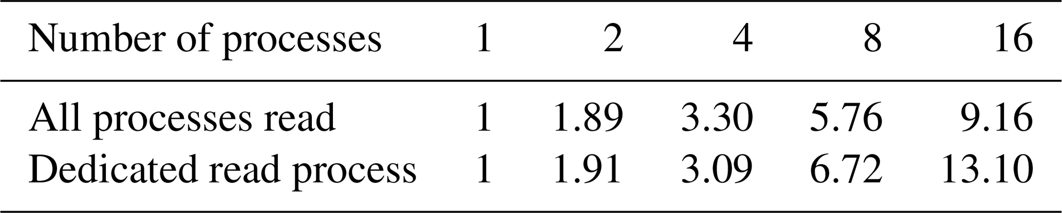
Next we repeated the experiment above but set aside a dedicated process for reading the meteorological data whenever n≥4. The results are shown in Fig. 7b and d. Numerical values for the speedup factors for selected numbers of processes are given in Table 3. We observed that with n≥7 there was consistently a benefit to setting aside the dedicated reader process, whereas for n<7 it was more effective to have all processes read data and thus an extra process available for doing the trajectory calculations. These results will of course vary with the resolution of the input data, the number of particles and the system on which the program is run.

Table 3 Computational speedup S for up to 16 processes (single-node experiment) for the two different MPI modes, with 40 million released particles.

3.2.2 500 million particles, multiple 16-core nodes

We performed a larger-scale experiment at the Abel computer cluster¹ using up to 256 cores on 16 nodes with Intel Xeon E5-2670 CPUs. For each node, up to 16 cores were used, and then the number of nodes was determined by the total number of processes launched. The FLEXPART setup was similar to the previous single-node experiment, but we increased the number of particles to 500 million and reduced the simulated time to 12 h. Compilation was done with Intel Fortran v16.0.1 and OpenMPI v1.10.2.

Run time and speedup factors are shown in Table 4 and Fig. 8. As before we see essentially perfect speedup of the computationally intensive parts (the particle loops), which is expected. Table 4 also gives the parallel efficiency, which is seen decreasing for larger N_p. This is partly due to the increased cost of MPI communications and also because the nonparallel parts of the code have relatively higher impact. With 256 processes there are only about 2 million particles per process and the CPU time is not as clearly dominated by the particle loops as when 500 million particles all run in one process. In addition, the initialization of the code (allocation of arrays, reading configuration files) takes around 20 s for this run, which is significant given a total run time of 299 s. Thus, parallel efficiency would increase for longer simulation times and/or for simulations with more particles per process, i.e., realistic cases that are more likely to be run with such a large number of processes.

Table 4 Run time and speedup for the multi-node experiment with 500 million particles. Up to 16 nodes in the Abel cluster (University of Oslo).

^* Superlinear speedup (efficiency greater than 100 %) as seen here is usually attributed to memory and/or cache effects.

3.2.3 900 000 particles, laptop and single 16-core node

Finally, we examined a small-scale experiment in which we released 900 000 particles and simulated 15 d of transport. The performance was tested on two systems; a ThinkPad P52s laptop (Intel i7-8550U CPU with four cores; results in Table 5) and a machine equipped with an AMD Opteron 6386 SE processor (16 cores; results in Table 6). With this relatively lower number of particles it is not surprising to see that the parallel efficiency is lower than in the preceding examples. Still, we see that a speedup of 2.38 on a 4-core laptop and 5.25 on a 16-core machine is attainable. We also note that for practical applications, users would likely use the serial version for applications with so few particles and, if there are many such runs to be done, use trivial parallelization by submitting many separate serial runs in parallel. The parallelization feature is most useful for cases with a very large number of particles that cannot so easily be split in many separate runs, such as domain-filling simulations.

Table 5 Run time and speedup using up to four cores on a ThinkPad P52s laptop (900 000 particles).

Table 6 Run time and speedup using up to 16 cores on a machine equipped with an AMD Opteron 6386 SE processor (900 000 particles).

3.3 Validation

In order to ensure that the parallel version produces results with the same accuracy as the serial version, we have performed a set of tests and validation experiments. A direct comparison between the versions can only be performed in statistical terms because FLEXPART uses Gaussian-distributed random numbers for calculating the turbulent velocities of the particles. For the parallel version we let each process independently calculate a set of random numbers, which leads to small numeric differences (arising from the random “noise”) between the versions.

To confirm that the only source of differences between the serial and parallel code is in the random number generation, we first observe that when the parallel executable is run using only one process, it produces results identical to the serial version. This is as expected, as the first MPI process (rank 0) always uses the same random number seeds as the serial version.

Next, we have done tests in which all random numbers are set to zero in both codes, corresponding to switching off the turbulent displacements, and we run the parallel version using multiple processes. The outputs from the serial and parallel versions of the code when run this way are identical except for small differences due to round-off errors (e.g., in concentration calculations – these round-off errors are typically larger in the serial version due to the larger number of particles).

4 Installation, compilation and execution

FLEXPART is usually used in a Linux environment, which we also assume for the following instructions. However, the model has also been implemented successfully under MacOS and MS Windows. The default Fortran compiler for FLEXPART v10.4 is gfortran, but ifort, Absoft and PGI compilers have been used as well.

4.1 Required libraries and FLEXPART download

As the meteorological data from numerical weather prediction models are usually distributed in GRIB format, a library for reading GRIB data is required. It is recommended to use ecCodes (https://software.ecmwf.int/wiki/display/ECC, last access: 30 October 2019), the primary GRIB encoding–decoding package used at the ECMWF (recent enough versions of its predecessor grib_api, no longer supported after 2018, can also be used). Data in GRIB-2 format can be compressed. If this is the case for the input data, the jasper library is needed². If it is desired to produce FLEXPART output in the NetCDF format, the NetCDF Fortran Library (https://www.unidata.ucar.edu/software/netcdf/, last access: 30 October 2019) is also required.

In order to obtain the FLEXPART source code, download the appropriate v10.4 tarball from the FLEXPART website³ and unpack it.

tar -xvf flexpart10.4.tar

To obtain the latest available model version, clone the FLEXPART git repository from the FLEXPART community website.

git clone https://www.flexpart.eu/
gitmob/flexpart

This repository mirrors https://transport.nilu.no (https://git.nilu.no/flexpart/flexpart/-/releases, last access: 18 November 2019). Additional mirrors exist, e.g., at GitHub (https://github.com/flexpart/flexpart, last access: 30 October 2019) and BitBucket (https://bitbucket.org/flexpart/flexpart, last access: 30 October 2019). See the “Code and data availability” section for additional information. After unpacking the tarball or cloning the repository, a local directory structure as shown in Table 1 is created.

The directory src contains the code and a makefile. The makefile needs to be adapted to the compiler and libraries present on the local system. Appendix A4 describes these steps in detail, including manual installation of the libraries. This was tested for Ubuntu 16.04.3 as well as 18.04.3 LTS Linux and MacOS (OS versions 14.5.0 and 18.6.0). Both a serial and a parallel executable can be built from the FLEXPART v10.4 source files.

4.2 Compiling and running the serial version

After correctly setting the library paths in the makefile, the command make produces the executable called FLEXPART. It can be executed from the command line by ./FLEXPART and then expects a file pathnames to exist in the current working directory. This file contains information on where input data are located and where output data shall be produced (see Sect. 5). Note that pathnames is expected in the directory from which FLEXPART is started, which can be different from where the executable file is located. A different name of a pathnames file can be also given as an argument. FLEXPART can thus be invoked according to the following generic syntax:

path_to_flexpart/flexpart_executable
path_to_pathnames/pathnames_file.

Using an optional argument, -v (verbose mode), will display additional information during the run. Even more information, including clock time between different program units, will be printed with -v2. Invoking FLEXPART with the flags -i and -i2 (info mode) will provide detailed run-specific information while reading input files. However, in this mode FLEXPART then stops before particle trajectories are calculated.

4.3 Compiling and running the parallel version

Most subroutines calling MPI functions are in a single module named mpi_mod.f90. Other FLEXPART source files that depend on this module are given the _mpi.f90 suffix to distinguish them from the serial version. During compilation the makefile selects the source files automatically depending on whether the parallel or serial version is built.

In order to compile and run the parallel version, an MPI library must be installed, either as a package from the distribution or built from source code. Both OpenMPI (http://www.open-mpi.org/software/ompi/v1.8/, last access: 30 October 2019) and mpich2 (http://www.mpich.org/downloads/, last access: 30 October 2019) work, but testing on some systems indicates slightly better performance with OpenMPI. As for the other libraries, the MPI library names and paths need to be adapted in the makefile. The MPIF90 variable sets the Fortran compiler wrapper (usually mpifort or mpif90; in the case of coexisting OpenMPI and mpich installations, wrappers called mpif90.openmpi or mpif90.mpich may be defined). Compilation of the parallel version should then be done by the following.

make mpi

This will produce an executable file FLEXPART_MPI. If executed, this will run on a single processor and should produce results identical to the serial version. To activate the parallel features, the executable must be run through an MPI launcher (here it is important to use the launcher corresponding to the MPI library that was used for the compilation).

mpirun -n <number> FLEXPART_MPI

In this example, <number> specifies the number of processes one wishes to launch. For some installations, mpirun is called mpiexec, or, in the case of coexisting OpenMPI and mpich2 installations, mpiexec.openmpi or mpiexec.mpich2, respectively. Many command-line options exist for mpirun that can be helpful for improving performance, e.g., processor binding. For a list of these options, see mpirun --help. In practice, the optimal number of cores for a given simulation will depend on the size of the problem and the hardware availability among other factors.

5 FLEXPART input

In this section, we describe the different FLEXPART input files and, where appropriate, changes that have occurred since the last publication (Stohl et al., 2005). FLEXPART needs the following three types of input files.

1. The text file pathnames is located by default in the directory where FLEXPART is executed. It must contain at least four lines: first, the path to the directories where run-defining input files are located (the so-called options directory); second, the path where output files are created; third, the path to the meteorological input GRIB files; and, fourth, the path to the so-called AVAILABLE file (see point 3). The last two lines can be repeated if nested input data shall be used. For each nesting level, one line for the GRIB data directory and one for the corresponding AVAILABLE file are needed.

2. The files containing the run-defining settings are located in a subdirectory (given in line 1 of pathnames) by default called options (see Table 1). The settings, which control FLEXPART's physics and program flow, are stored in different text files listed in Table 7 and described in Sect. 5.1. In addition, the options directory contains data files that are not usually changed by the user.

3. The meteorological input data, one file for each input time, are stored in GRIB format in a common directory (specified in line 3 of pathnames). To enable FLEXPART to find these files, a file usually named AVAILABLE (given in line 4 of pathnames) contains a list of all available meteorological input files and their corresponding time stamps. Additional files containing nested input data may also be provided. In this case, a separate file containing the input file names (e.g., named AVAILABLE_NESTED) must be given. Date and time entries in the AVAILABLE* files for mother and nested fields must be identical. Details on the meteorological input data are given in Sect. 5.2.

Table 7 Alphabetical list of the run-defining input files (upper part) and static input files (lower parts), usually contained in a directory called options. Processing of files marked with ^* depends on the run specifications. The other files are always read in.

5.1 Run-defining settings: the options directory

Here, we give an overview of the information provided in the run-defining FLEXPART user input files listed in Table 7. In previous versions of FLEXPART, these files were formatted text files (coming alternatively in a long and a short format). For backward compatibility, these plain text formats are still supported. However, FLEXPART v10.4 also allows for the use of namelists, a standard Fortran feature whereby values are provided in a list with elements of the form name=value. When FLEXPART is started, it tries to open the files as namelists, and if this is not working, it expects the files to be in one of the two old plain text formats. We encourage users to update their input files to namelists for two reasons. Firstly, FLEXPART now has default user options for all input settings so that users only need to set those options that they want to deviate from the defaults. Secondly, namelists make it easier to add new user options, which may be required in future versions of FLEXPART. Thus, plain text input files may not be supported in future versions of FLEXPART. Examples for all formats of the user input files are contained in the FLEXPART distribution.

To convert user input files of any format to namelist format, the switch nmlout=.TRUE. (in file com_mod.f90) must be set before compilation. Then, run-defining user input files are written out in namelist format in the output directory, with the appendix .namelist added to the input file name (e.g., COMMAND.namelist). This feature also improves the traceability of FLEXPART model results and makes simulations easily reproducible by documenting the settings used for the model run.

In the following, we provide reference tables of the run-defining user input files including default settings (in bold) when using the namelist format. Notice that the default values are appropriate for regional-scale simulations, but simulations on smaller scales or with higher accuracy may need adjustments (in particular, shorter time steps and the use of the new CBL scheme).

5.1.1 File COMMAND

The COMMAND file contains the user settings controlling the simulation and the behavior of the run. The default COMMAND file contains a namelist &COMMAND, for which Table 8 provides a complete listing of all settings with their meaning and preset default values. It is important that users of previous FLEXPART versions who choose to use plain text input files update their COMMAND file, since new parameters have been added. However, the cblflag (and any option added afterwards) must be provided in namelist format in any case.

Seibert and Frank (2004); Eckhardt et al. (2017)Seibert and Frank (2004); Eckhardt et al. (2017)

Table 8 Contents of the user input file COMMAND. Variable names with their meaning and all possible values are listed. Where appropriate, default values are given in bold. Note that not all input parameter combinations are allowed.

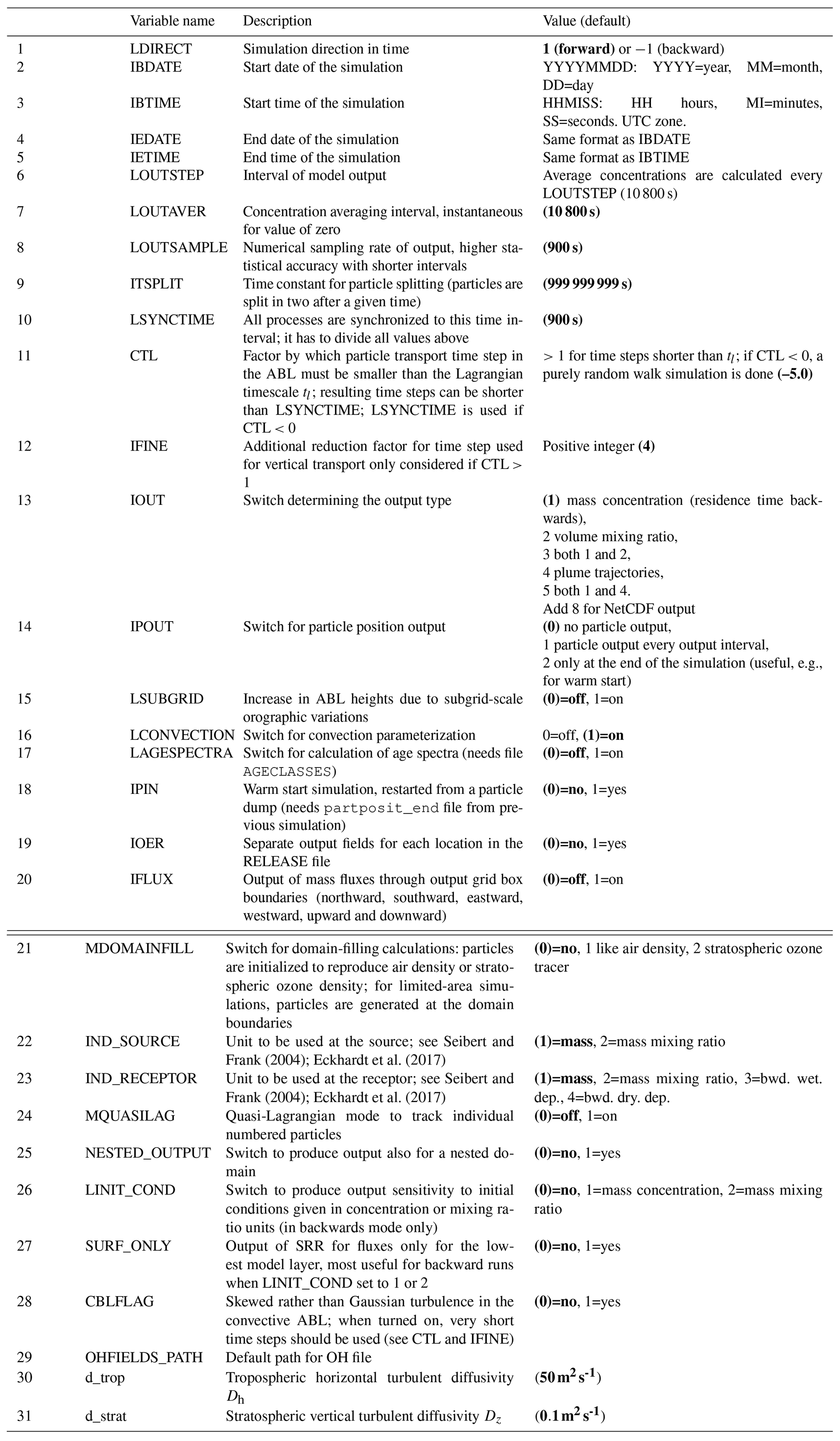
5.1.2 File RELEASES

The RELEASES file contains information related to when and where the particles are introduced in the simulation and other properties of the release points (e.g., the chemical species simulated). It consists of a namelist &RELEASES_CTRL that specifies header information. The header gives the total number of different species (i.e., different substances) to be released, followed by a corresponding list of the FLEXPART species numbers nnn, and SPECIES_nnn files define the species' physical properties (see Sect. 5.1.3). Following the header, there is an arbitrary number of namelists &RELEASE defining each release. For each such release, the following is given: the starting and ending time, the location and extension, the masses released (one value for each released species), and the number of particles to be released, as well as a comment string. The content of the RELEASES file is summarized in Table 9.

Table 9 Contents of the user input file RELEASES.

5.1.3 SPECIES files

The subdirectory options/SPECIES/ needs to contain one or more files named SPECIES_nnn. For each species nnn listed in the header section of the RELEASES file, such a SPECIES_nnn file must exist. The parameters in the SPECIES_nnn file, contained in the namelist &SPECIES_PARAMS, set the species name and define the physicochemical properties of the species; they are described in Table 10. These are important for simulating radioactive or chemical decay, wet deposition (scavenging) for gases and aerosols, dry deposition for gases and aerosols, particle settling, and chemical reaction with the OH radical. Some parameters are only necessary for gas tracers and some are only necessary for aerosol tracers; thus, a namelist does not need to contain all parameters for both gases and particles. Optionally, since FLEXPART version 6.0, information about temporal emission variations can be added at the end of the file.

Notice that the format of the SPECIES_nnn files has changed from previous FLEXPART versions and users need to update their files accordingly. The use of SPECIES_nnn files from older FLEXPART versions may lead to run time errors or erroneous results.

Table 10 FLEXPART variables set in the user input file SPECIES_nnn for species number nnn. Note that the variable names given in the input namelist are the same as used subsequently in FLEXPART but with a prepended letter p (for parameter). For instance, pspecies corresponds to species.

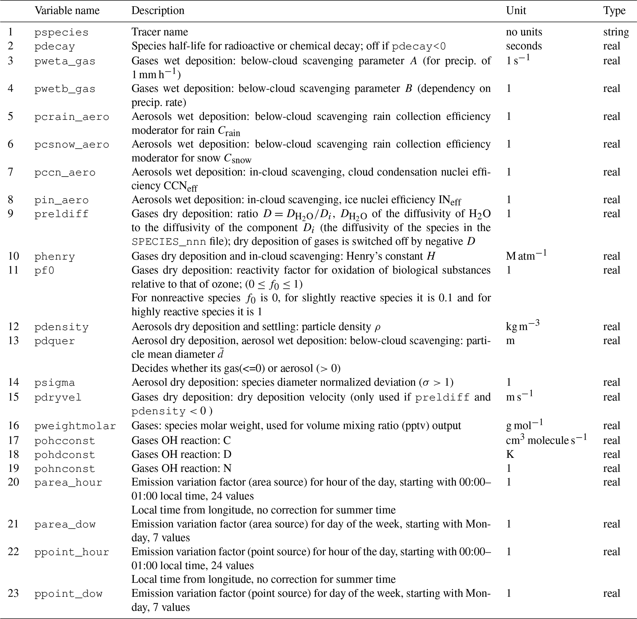
The following specifies the parameters associated with each physicochemical process simulated.

• Radioactive or chemical decay: set with pdecay; off if pdecay<0.

• Wet deposition for gases: set with pweta_gas, pwetb_gas (for below-cloud) and phenry (for in-cloud). Switch off for both in- and below-cloud if either pweta_gas or pwetb_gas is negative.

• Wet deposition for aerosols: set with pccn_aero, pin_aero for in-cloud scavenging and pcrain_aero, pcsnow_aero and pdquer for below-cloud scavenging.

• Dry deposition for aerosols: set with pdensity, pdquer and psigma; off if pdensity<0.

• Dry deposition for gases: set with phenry, pf0 and preldiff; off if preldiff<0. Alternatively, a constant dry deposition velocity pdryvel can be given.

• Settling of particles: set with pdensity and pdquer.

• OH reaction: chemical reaction with the OH radical can be turned on by giving parameter pohcconst (cm³ molecule⁻¹ s⁻¹), pohdconst (K) and pohnconst (no unit) positive values; defined by Eq. (13).

• Emission variation: emission variation during the hours (local time) of the day and during the days of the week can be specified. Factors should be 1.0 on average to obtain unbiased emissions overall. The area source factors (useful, e.g., for traffic emissions) are applied to emissions with a lower release height below 0.5 m above ground level (a.g.l.) and the point source factors (useful, e.g., for power plant emissions) to emissions with a lower release height than 0.5 m a.g.l. Default values are 1.0.

5.1.4 File OUTGRID

The OUTGRID file specifies the domain and grid spacing of the three-dimensional output grid. Note that in a Lagrangian model, the domain and resolution of the gridded output are totally independent from those of the meteorological input (apart from the fact that the output domain must be contained within the computational domain). The OUTGRID file contains a namelist &OUTGRID specifying all parameters. The variables read in for this file and all the following input files have not changed in recent FLEXPART versions; thus, for further explanation, see Stohl et al. (1995). Example files can be found in the options directory in the FLEXPART distribution.

5.1.5 File OUTGRID_NEST

Output can also be produced on one nested output grid with higher horizontal resolution, defined in the file OUTGRID_NEST, but with the same vertical resolution as given in OUTGRID. The OUTGRID_NEST file contains a namelist &OUTGRIDN specifying all parameters.

5.1.6 File AGECLASSES

The option to produce age class output can be activated in the COMMAND file. The file AGECLASSES then allows for the definition of a list of times (in seconds, in increasing order) that define the age classes used for model output. With this option, the model output (e.g., concentrations) is split into contributions from particles of different age, defined as the time passed since the particle release. Particles are dropped from the simulation once they exceed the maximum age, allowing their storage locations to be reused for new particles. This is an important technique to limit the memory usage for long-term simulations. Thus, even if the user is not interested in age information per se, it may often be useful to set one age class to define a maximum particle age.

5.1.7 File RECEPTORS

In addition to gridded model output, it is also possible to define receptor points. With this option output can be specifically produced for certain points at the surface in addition to gridded output. The RECEPTORS file contains a list with the definitions of the receptor name, longitude and latitude. If no such file is present, no receptors are written to output.

5.1.8 Static data input files

Several files contain static input data that are not usually modified by the user. These are (by default) also located in the options directory. If modeling a species requires calculating OH reactions, an OH field stored in file OH_variables.bin needs to be present. The file IGBP_int1.dat is a land cover inventory; file surfdata.t gives the roughness length and leaf area index of the different land cover types, and file surfdepo.t contains surface resistances for dry deposition calculations.

5.2 Meteorological data and preprocessing routines

FLEXPART can be run with meteorological input data for global domains or for smaller, limited-area domains. The FLEXPART computational domain always corresponds to this mother domain set by the input data, while the output domain can be smaller. FLEXPART can also ingest higher-resolution meteorological input data in subdomains of the mother domain. Such nested data must be available for the exact same times as those for the mother domain, checked by FLEXPART by comparing the time stamps in the two AVAILABLE(_NESTED) files. There is no nesting in the vertical direction and the poles must not be contained in any nest. To automatically produce the AVAILABLE(_NESTED) files, a Python script is available from the FLEXPART website (https://flexpart.eu/wiki/FpInputMetMkavail, last access: 25 June 2018) that checks which input files are present and then creates this file in the required format.

Compilation of FLEXPART v10.4 produces a single executable that automatically detects whether the meteorological input data come from the ECMWF IFS or NCEP GFS and whether they are in GRIB-1 or in GRIB-2 format. Nevertheless, certain parameters may need to be adapted in par_mod.f90 to the size of the meteorological input files (array dimensions), and the input grid may need to be shifted relative to the output grid (parameter nxshift). In the following, we describe how meteorological input data appropriate for FLEXPART can be retrieved from the ECMWF and NCEP.

5.2.1 ECMWF data retrieval

ECMWF data can be comprised of analysis and/or forecast data from the operational IFS data stream or specific reanalysis projects. For operational data, the meteorological fields can currently have a maximal temporal resolution of 1 h (more frequent data are not available), a vertical resolution of 137 model levels and $\mathrm{0.1}{}^{\circ }\times \mathrm{0.1}{}^{\circ }$ horizontal resolution on a regular latitude–longitude grid. Other ECMWF datasets are not available at such high horizontal resolution. For example, ERA-Interim reanalysis data (Dee et al., 2011) with $\mathrm{1}{}^{\circ }\times \mathrm{1}{}^{\circ }$ latitude–longitude resolution and 60 vertical levels can be retrieved 3-hourly by mixing 6-hourly analysis and 3 h forecast fields, but higher resolution is not available from the standard archive. The new Copernicus reanalysis ERA5 provides 1-hourly analysis fields with 137 model levels and a horizontal resolution of 31 km (0.28125^∘). Notice that access to some datasets, in particular the operational forecasts, is restricted and requires specific access (https://www.ecmwf.int/en/forecasts/accessing-forecasts, last access: 23 June 2018). However, reanalysis data (https://software.ecmwf.int/wiki/display/WEBAPI/Available+ECMWF+Public+Datasets, last access: 23 June 2018) are publicly available.

The IFS is a global model that uses spectral representation with spherical harmonics for the dynamical part and a grid-point representation on a reduced Gaussian grid for the physical part. However, FLEXPART needs the input data on a regular latitude–longitude grid, and thus IFS data have to be preprocessed. With respect to the vertical coordinate system, the data need to be on the native ECMWF model levels (η levels), which are subsequently transformed within FLEXPART to a terrain-following vertical coordinate system.

As explained above, each ECMWF dataset has its own specific temporal and spatial resolution, and the meteorological parameters provided can be different from dataset to dataset. To produce meteorological GRIB files suitable for FLEXPART input from these different datasets, a software called flex_extract (current version 7.0.4) has been developed specifically for this purpose. In order to prepare the GRIB files from the ECMWF Meteorological Archival and Retrieval System (MARS; https://software.ecmwf.int/wiki/download/attachments/45759146/mars.pdf, last access: 24 June 2018), several retrieval requests using the MARS command language and some further processing steps are needed. Since all ECMWF datasets need to be handled differently and some may not even contain all information needed for FLEXPART, flex_extract has a focus on some of the most important ones for driving FLEXPART. These are, in particular, the reanalysis datasets ERA-Interim (Dee et al., 2011), CERA-20C (the coupled climate reanalysis of the 20th century; Laloyaux et al., 2018) and the latest reanalysis ERA5, as well as data from the operational IFS stream. Each file (one for each time step) prepared by flex_extract for FLEXPART consists of a set of model-level and surface data as a combination of analysis and forecast fields depending on availability. For example, certain variables such as precipitation may only be available in forecast fields, whereas other data are also contained in analysis fields; flex_extract seeks an optimum combination of such data. Note that some parameters are stored as time-accumulated fields in the ECMWF archives and flex_extract calculates the instantaneous fluxes out of them (e.g., precipitation fluxes). For more details on this process of de-accumulation, see Hittmeir et al. (2018). Since FLEXPART needs the pressure hybrid coordinate vertical velocity as used in the ECMWF model, an important feature of flex_extract is the computation of this parameter from the horizontal wind field (see Stohl et al., 2001) for ERA-Interim and for the years when it was not operationally archived in MARS (before 2009).

The ECMWF is a European intergovernmental organization that grants full access to its multi-petabyte MARS archive for their member and cooperating states. Users with a full-access account can run flex_extract v7.0.4 directly on ECMWF servers or via a local gateway server. This mode is also required to retrieve the most recent operational data from the ECMWF. Users from member or cooperating states interested in this mode should contact the computing representative from their national meteorological service to obtain an account. Users from other countries worldwide can self-register at the ECMWF for a public account to be able to retrieve the public datasets (i.e., most reanalysis products); flex_extract v7.0.4 makes use of the WebAPI (https://software.ecmwf.int/wiki/display/WEBAPI/ECMWF+Web+API+Home, last access: 24 June 2018) tool provided by the ECMWF to access the data from outside their systems. This tool can distinguish between public and member state users. Therefore, it is also a convenient option for member and cooperating state users who only need data older than a few days from the operational stream or reanalysis data. A full-access account to ECMWF servers is no longer needed in this case.

The flex_extract software v7.0.4 is a set of Python routines combined with a Fortran program for faster computation of grid transformations and vertical velocity calculation. A Python 2.7 interpreter with several common modules, such as NumPy and date–time, are required and usually included in the Anaconda distribution (https://www.anaconda.com/download/, last access: 25 June 2018). Additionally, a Fortran compiler, the ECMWF WebAPI tool, the GRIB-API or ecCodes module, and the Emoslib interpolation library have to be available. Note that the GRIB-API (or ecCodes) module has to be available for Python as well as for Fortran. Installation instructions can be found at ECMWF websites directly or in the Software Installation Plan for flex_extract. Knowledge of Python, although helpful, is not necessary for using the retrieval scripts. A certain knowledge of the ECMWF dataset to be retrieved is useful to understand the composition of retrievals, but many basic examples of CONTROL files are provided in the flex_extract distribution. These CONTROL files determine the key parameters for the flex_extract MARS retrievals and can be adapted to change domain as well as spatial and temporal resolution. Even for these few parameters the user should check for availability upfront. For example, ERA-Interim data have a maximum grid resolution of $\mathrm{0.75}{}^{\circ }\times \mathrm{0.75}{}^{\circ }$ and 6-hourly temporal resolution for the public dataset.

The flex_extract v7.0.4 software is included in the FLEXPART v10.4 file tree under the directory preprocess (see Table 1). It can also be downloaded from https://flexpart.eu/ (last access: 30 October 2019) (https://flexpart.eu/downloads/62, last access: 30 October 2019) as a tarball. For more details the reader is referred to the flex_extract v7.0.4 user documentation (e.g., the Software Installation Plan – SIP.pdf – and the Software User Tutorial – SUT.pdf) in preprocess/flex_extract.

5.2.2 NCEP data retrieval

Meteorological data from the NCEP GFS are freely available, easily accessible and ingested by FLEXPART on pressure levels, unlike ECMWF data. These pressure-level data have lower resolution than model-level data but offer the advantage of great consistency between different datasets. Therefore, preprocessing NCEP data is much simpler than ECMWF data and limited to precipitation data, which are available only in forecast fields.

Both operational analysis data and several reanalysis datasets are available. Notice that NCEP also provides forecast data for free, which are not available from the ECMWF even for member state users except for national meteorological services or users with a special contract. The data retrieval from NCEP is described in a wiki page on the FLEXPART website (https://flexpart.eu/wiki/FpInputMetGfs, last access: 8 July 2018), where a script for downloading NCEP data can also be found. Operational GFS data can be downloaded by simple FTP or wget from a rolling archive of the meteorological forecast and analysis data (http://www.ftp.ncep.noaa.gov/data/nccf/com/gfs/prod/, last access: 8 July 2018) under the catalog gfs.YYYYMMDDHH, which contains fields in GRIB-2 format. Six-hourly NCEP FNL (Final) Operational Model Global Tropospheric Analyses (http://rda.ucar.edu/datasets/ds083.2/, last access: 30 October 2019) are available in near-real time since July 1999. These data are similar to the operational analyses, but NCEP also ingests late-incoming observation data for their production. Archived reanalysis datasets are also available from NCEP, e.g., the Climate Forecast System Reanalysis (CFSR) Selected Hourly Time-Series Products (http://rda.ucar.edu/datasets/ds093.1/, last access: 30 October 2019) for the period January 1979 to March 2011.

6 FLEXPART output

6.1 Output files overview

In the following we describe the FLEXPART output files together with changes made since the last documented FLEXPART version (Stohl et al., 2005). An overview of all possible output files is provided in Table 11. Notice that not all these files are written out in every model run; the user settings control which files are produced. At the beginning of a run, FLEXPART records descriptive metadata in the binary file header. This information is also written into the plain text files header_txt (with the exception of the orography data and release information). The release information is written in header_txt_releases. Corresponding files header_nest are produced if nested output is selected.

Table 11 List of FLEXPART output files and for which user settings (“switches”) they are produced. See Table 12 for details on the units in the gridded output.

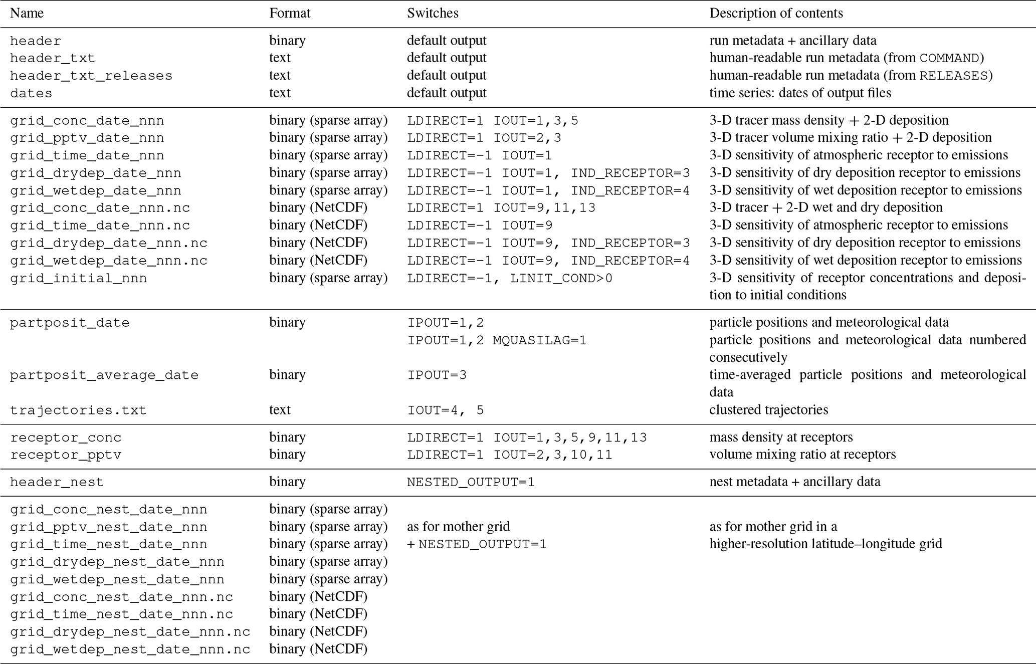
At each output time, FLEXPART produces files containing the gridded output. Separate files are created for every species and domain (mother and, if requested, nest). The naming convention for these files is grid_type_date_nnn. For forward runs, type can be conc or pptv for concentrations and mixing ratios or flux for 3-D mass fluxes across the grid cell faces (Stohl et al., 2005, Sect. 8.5). For backward runs, type can be time for the sensitivity of receptor concentrations to emission fluxes, drydep for the sensitivity of receptor dry deposition to emissions or wetdep for the sensitivity of receptor wet deposition to emissions. For backward runs, there can also be an output file grid_initial_nnn, which gives the receptor sensitivity to initial conditions; date denotes the date and time for which the output is valid, and nnn is the species number as specified in RELEASES. The list of the output times is progressively written to the text file dates. For the nested output, grid is replaced by grid_nest.

Wet and dry deposition fields in forward runs are calculated on the same horizontal output grid and are appended to grid_conc_date_nnn and grid_pptv_date_nnn files. The deposited matter is accumulated over the course of a model run. It generally increases with model time, but for species with radioactive decay, losses are possible. As for long simulations small deposition amounts may be added to already large deposited quantities, the default precision of the deposition fields was changed from single (in older FLEXPART versions) to double precision to avoid numerical inaccuracies when deriving instantaneous fluxes from accumulated quantities.

For a list of points at the surface, concentrations or mixing ratios in forward simulations can also be calculated independently from the grid using a kernel method and recorded in the files receptor_conc and/or receptor_pptv.

If the particle dump option is activated, in addition to the gridded output, the particle coordinates together with additional variables such as pressure, humidity, density, tropopause height, ABL height and orography height are recorded in the binary files partposit_date. These data can be useful for a variety of different purposes, for instance diagnostics of the water cycle (Stohl and James, 2004). FLEXPART version 10.4 also has the new option to write out time-averaged particle positions and meteorological data. These are recorded in the files partposit_average_date. Such output may be useful to obtain, for instance, more representative heights for particles in the boundary layer, where particle positions change rapidly and this is not sampled sufficiently with instantaneous output. If plume trajectory mode is activated, for every release the positions of trajectory clusters representing the centers of mass of all released particles are recorded in the file trajectories.txt (Stohl et al., 2002, 2005, Sect. 10).

The physical unit used for the output data in the files grid_conc_date_nnn and grid_time_date_nnn depends on the settings of the switches ind_source and ind_receptor, following Table 12. It is noteworthy that the unit of mass mixing ratio can also be used in grid_conc_date_nnn. For forward runs, additional files grid_pptv_date_nnn can be created (setting IOUT to values of 2 or 3), which contain data such as volume mixing ratios (requires molar weight in SPECIES_nnn file). Source–receptor relationships (i.e., emission sensitivities) in backward mode for atmospheric receptors are written out in grid_time_date_nnn files; those for deposited mass are recorded in files grid_wetdep_date_nnn and grid_drydep_date_nnn (see Seibert and Frank (2004), Eckhardt et al. (2017), Sect. 2.5, and Table 12 for output units). Notice that the user can also provide different input units. For instance, if emissions in a forward run are specified in Becquerels (Bq), the output would be in nanobecquerels per cubic meter (nBq m⁻³) with ind_source=1 and ind_receptor=1. Notice further that all gridded output quantities in FLEXPART are grid cell averages, not point values.

Table 12 Physical units of the input (in file RELEASES) and output data for forward (files grid_conc_date_nnn) and backward (files grid_time_date_nnn) runs for the various settings of the unit switches ind_source and ind_receptor (for both switches, 1 refers to mass units, 2 to mass mixing ratio units). IOUT is 1 (or 9 for NetCDF output) except where indicated; “(dep.)” in lines 5 and 6 of the table refer to the deposition output provided in addition to the atmospheric output in files grid_conc_date_nnn.

6.2 Sparse matrix output

Depending on the type of model run, the gridded output can contain many grid cells with zero values (e.g., dispersion from a point source, backward run from a single receptor). The output is therefore written in a sparse matrix format, which is specific to FLEXPART. The array containing the data to be written out is scanned for sequences of nonzero values. The number of sequences found is stored in an integer variable sp_count_i, and the field positions at which each sequence begins are stored in a 1-D integer array, sparse_dump_i, using a one-dimensional representation of the output field. The total number of nonzero values is stored in sp_count_r and the nonzero values themselves in the real vector sparse_dump_r. Since all physical output quantities of FLEXPART are greater than or equal to zero, nonzero sequences are stored in sparse_dump_r with alternating signs, which allows for the separation of different sequences upon reading. Finally, all four variables are written out to the unformatted output file. This format replaces the compression used up to version 7 (the smallest of a full dump and a simple sparse matrix format), saving up to 60 % of disk space. The sparse matrix data can be read, for example, with the functions readgrid.f (Fortran) and flex_read.m (MATLAB) described in Sect. 6.4

6.3 NetCDF output

FLEXPART v10.4 can also support output in NetCDF format if the NetCDF libraries are available. To activate NetCDF support, append ncf=yes to the make command. If FLEXPART is compiled and linked to the NetCDF libraries, output files in NetCDF format can be produced by adding 8 to the IOUT parameter in the input file COMMAND, e.g., IOUT=9 corresponds to IOUT=1 with the standard binary output; see Table 11 and Sect. 5.1.1. In the NetCDF module netcdf_output_mod.f90 a parameter write_releases determines at compile time if the information on the releases should also be written to the NetCDF file. Only one NetCDF file is written that contains all species and all time steps. Both mother and nested output (if present) are contained in that file. Since the NetCDF output is specified in the climate and forecast (CF) format, any standard software can be used for displaying and processing the output (e.g., panoply, ncview). NetCDF output data files are compressed.

The NetCDF output file contains information on the run settings and the simulation grid from the COMMAND and OUTGRID* files. It also contains additional information in the header on the producing center, as listed in Table 13. The content of these attributes can be adapted in the file netcdf_output_mod.f90 before compilation.

Table 13 Additional information in the NetCDF output file as attributes.

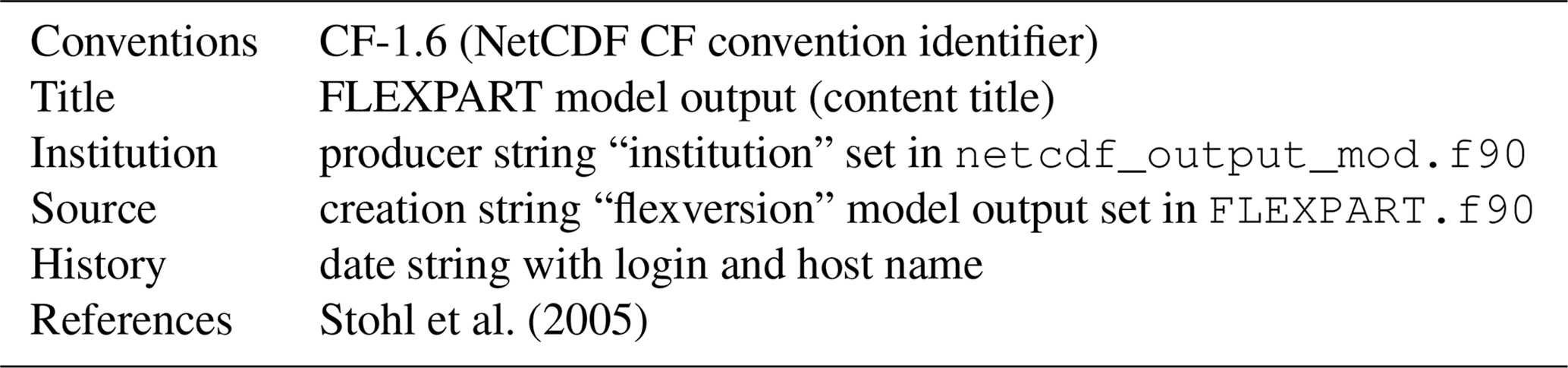
6.4 Post-processing routines

For the NetCDF output of FLEXPART, standard visualization tools, for example Panoply, can be used. For the sparse matrix binary output, several post-processing routines (MATLAB, Fortran, R, Python and IDL) have been developed in order to assist in the usage and analysis of these data. A number of post-processing tools are available online (https://flexpart.eu/wiki/FpOutput, last access: 16 August 2018). Note that some of these tools require reading a text string containing the model version. Since the length of this string changed in FLEXPART v9.2, the post-processing routines now require the allocation of a longer string.

Fortran routines are available for download on the FLEXPART website with the subroutines readheader.f for reading the header and readgrid.f for reading the gridded binary fields. Analysis or plotting programs written in Fortran can call these subroutines.

There are also MATLAB tools working in a similar way as the Fortran routines, with flex_header.m for reading the header and flex_read.m for reading the data fields. If particle dumps were made, the MATLAB function readpart.m reads the corresponding data files (a similar Fortran code is also available).

The R programs available for post-processing FLEXPART output include routines to read the binary output in the grid_conc (or grid_pptv) and grid_time files and to plot maps. Routines are also available to plot trajectories on a map from the file trajectories.txt and to plot time series of concentrations (or mixing ratios) from the file receptor_conc (or receptor_pptv).

Several Python tools are available for reading FLEXPART data from release 8.0 and above. The module reflexible, available from the FLEXPART website and also at https://github.com/spectraphilic/reflexible (last access: 6 August 2018), enables the user to easily read and access the header and grid output data of the FLEXPART model runs. It provides a simple tool that facilitates consistent reading of both the original sparse matrix output files and the NetCDF output. Some basic plotting functionality is provided to quickly assess and validate runs or to look at the input parameters. An alternative Python tool is Quicklook that can be also downloaded from the https://flexpart.eu website.

7 Application examples

In this section we provide 38 examples of the FLEXPART model that serve three purposes: (1) verification of a new FLEXPART installation; (2) demonstration of the model capabilities for new users; and (3) confirmation of consistency in the model output when code changes are made that should not change the results. These examples do not represent an exhaustive set of all possible model uses, but they are designed to demonstrate and test different widely used functionalities of the model.

All examples are variations of a default example case, which uses the settings in the user input files as distributed with the FLEXPART v10.4 code package. These default input files are located in the directory options (Sect. 5) and are consistent with the default meteorological data retrieved from the ECMWF by the flex_extract package (Appendices A5 and B1). An AVAILABLE file fitting with these input data is also distributed with FLEXPART. These default settings are described in detail in Appendix B2.

Using the default example as a basis, the different functionalities of the model can be activated by adequately changing certain parameters in the user input files, thereby generating 36 other example runs. We have categorized these examples into 10 different groups; each group explores different capabilities of the model. Table 14 lists all examples and the parameter changes needed to produce them. The first group includes the default example and explores the different options for producing gridded model output (e.g., output units, output formats) for a simple forward model run with a single starting point over the North Atlantic. The second group of examples introduces FLEXPART's backward simulation capability. The third group demonstrates different usages of the particle dump output. The fourth group gives examples for the use of mass vs. mass mixing ratio units at both the source and the receptor and for both forward and backward simulations to establish source–receptor relationships as in Seibert and Frank (2004). The fifth group produces output for different chemical species and aerosols. The sixth group illustrates the use of nested output fields. Group seven is constituted by a single domain-filling run, as used, for instance, in Stohl and James (2004). Group eight contains settings for a backward run providing 2-D sensitivities to gridded surface fluxes and 3-D sensitivities to initial conditions, as they are typically required for the inverse modeling of greenhouse gases (e.g., Thompson et al., 2017). Group nine shows the use of the new skewed turbulence parameterization (Cassiani et al., 2015). Group 10 shows the use of the new backward deposition (Eckhardt et al., 2017). Group 11 contains a forward 2 d run simulating instantaneous emissions from a hypothetical Grímsvötn eruption (Fig. 9).

Table 14 List of the test cases for FLEXPART 10.4.

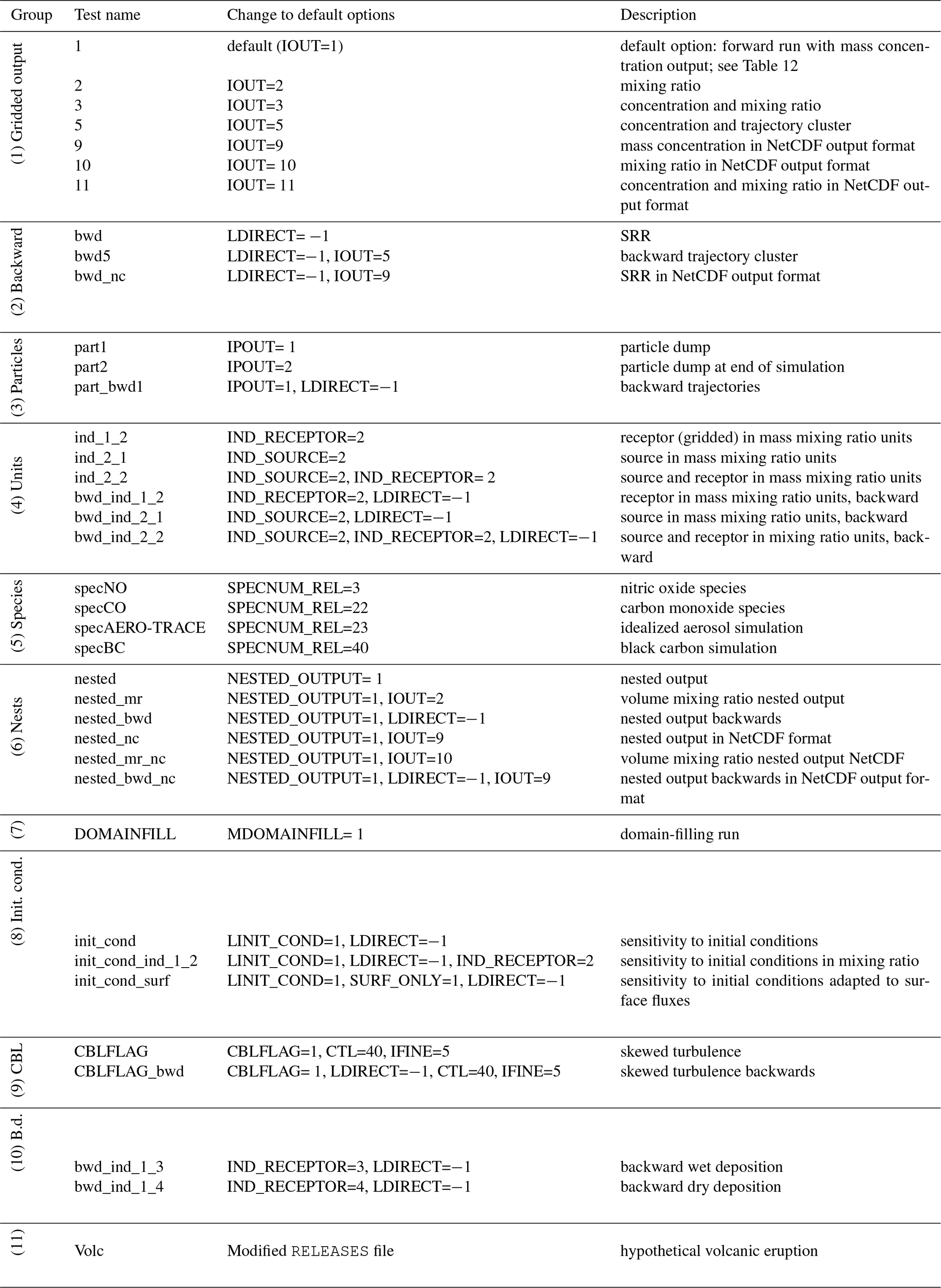
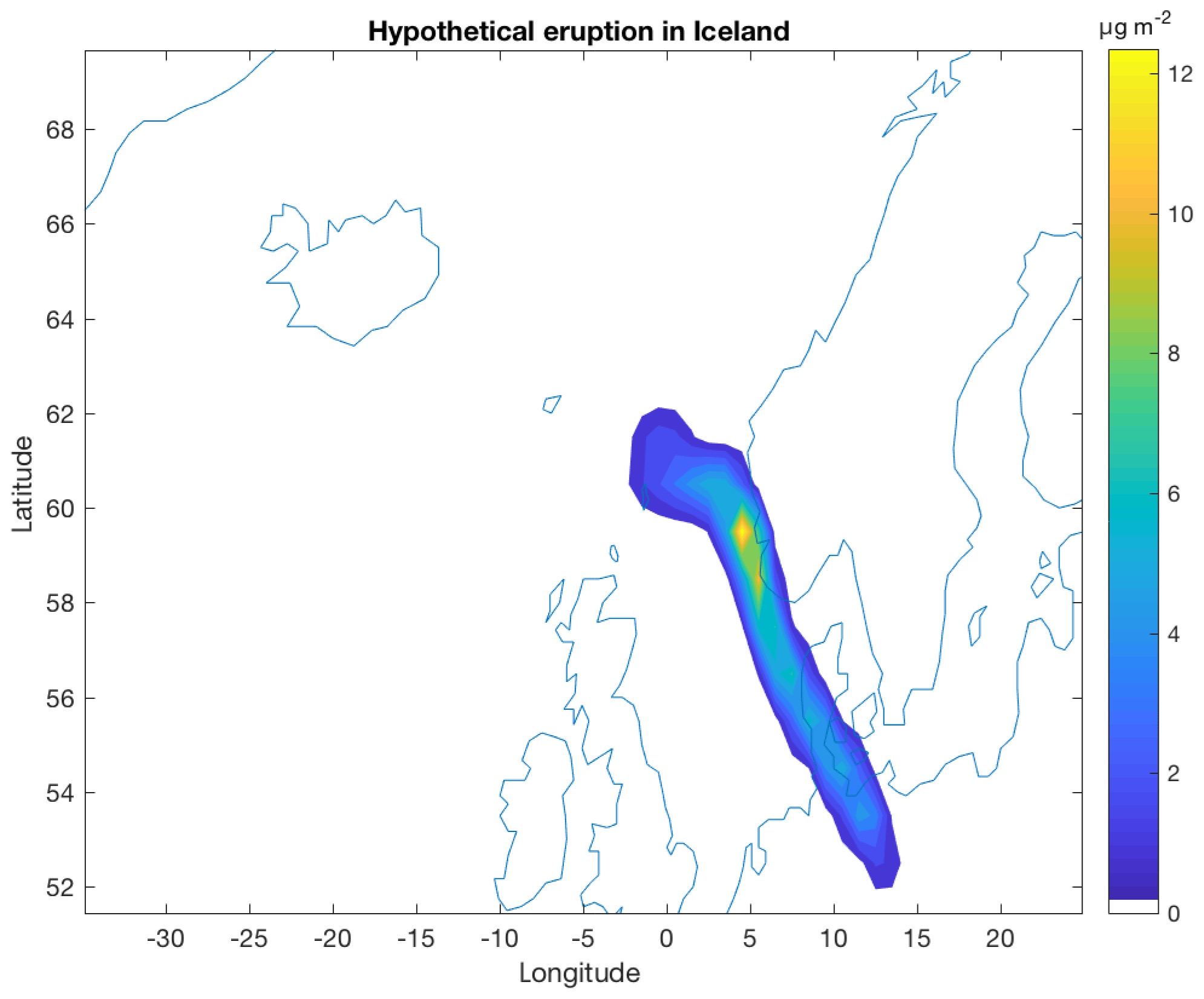
Figure 9 Hypothetical Grímsvötn eruption on 1 April 2015 at 00:00 UTC (instantaneous release). Total column concentrations are shown (µg m⁻²) 18 h after the eruption.

The list of examples may be extended in the future to allow for the testing of even more model features and to provide a reference archive to see how FLEXPART results may change as the code is being developed further. The user can get these reference results from https://flexpart.eu. A quick reference containing mean and maximum grid values for every example is also referenced in Appendix B5.

The directory tests/examples/ contains scripts that generate all the files necessary to run the examples. These scripts, described in Appendix B3, generate the input files by modifying the namelists in the default options directory provided with the distribution. This is done by the bash script gen_options_all.sh. For instance, the example “bwd” is generated by changing the line containing the parameter LDIRECT to −1 in the file COMMAND.

After the input data files are generated, all examples can be executed interactively from the command line. Alternatively, the script gen_batch_jobs_cl.sh generates a batch script for each case (to be run from the command line or using a workload manager such as SLURM). This procedure automates the sample output generation. Once the output files are created, they can be read using the tools in the directory postprocess. They can be plotted and analyzed with, e.g., the reading routines described in Sect. 6.4. In addition, some testing capabilities have been added. These are presented in Appendix B.

8 Final remarks, outlook and future code development

In this paper, we have described the Lagrangian particle dispersion model FLEXPART v10.4; 2 decades ago, the model code was developed mainly by one person, with specific code input from a few other researchers. At that time, no specific measures were needed to ensure code consistency, track code changes or identify coding bugs. However, as the number of FLEXPART users has grown substantially in recent years, more and more people have started to develop the code, contributed code snippets, and reported or identified bugs. The resulting code changes range from the adaptation of more modern coding standards, parallelization and efficiency enhancements, the improvement of the model functionality, and the addition of output options, to revisions and extensions of the model physics. All this has been documented in this paper. Integration of all these changes into a single stable model version represents a growing challenge in itself, and efforts to address this challenge (e.g., model website and repository, version control, testing environment) have also been documented here.

As FLEXPART is developed further, updates will continue to be made available on the FLEXPART website at https://flexpart.eu. We encourage established and new users to contribute to FLEXPART development by providing their code changes, as well as a description of these changes, as new feature branches of the latest commits in the FLEXPART git repository. New code should pass all test cases provided in the FLEXPART distribution and provide consistent output, unless there are specific reasons why output should be different, such as improvements in the model physics. This will expedite the integration of important new model features in the main development branch of the model.

Appendix A: Installing FLEXPART and flex_extract

Here, we provide step-by-step instructions on how to install FLEXPART on Linux from scratch. This has been tested on an Ubuntu 16.4 distribution running on a dedicated instance in the Amazon cloud. Notice that in most environments, some or all of the required libraries (e.g., a Fortran compiler) are already installed and an installation totally from scratch would thus not be needed. In such cases, we strongly recommend that these libraries are used instead of installing everything from scratch. However, sometimes it may be necessary to install them from source (e.g., to avoid incompatibilities between different compilers or different versions of the same compiler). In the following, we assume that the user has root privileges in the system, but it is also possible for normal users to install the libraries in nonstandard locations. It is possible to ask for help by writing to the FLEXPART user email list (registration needed) or by creating a ticket on the community website at https://flexpart.eu.

A1 System requirements

To begin, ensure that the latest packages are being used. This section is for completeness only, and most users (if not starting from a new system installation) can skip it and jump to Sect. A2.

sudo apt-get update

FLEXPART is developed using gfortran.

sudo apt-get install g++ gfortran

Some libraries (e.g., grib_api, jasper-1.900.1) require the GNU autotools suite in order to configure, build and install.

sudo apt-get install autoconf libtool
 automake flex bison

Newer packages (e.g., ecCodes) use CMake instead.

sudo apt-get install cmake

Python is not required for FLEXPART itself but is necessary for some preprocessing and post-processing tools, in particular flex_extract for retrieving ECMWF wind fields. Git is recommended to access the code repositories. An editor (e.g., vim) is usually also necessary.

sudo apt-get install python-dev
 python-pip git-core vim

A2 Installing GRIB libraries

If JPG compression is needed to decode the input meteorological winds, download the jasper library from the jasper project page (http://www.ece.uvic.ca/~mdadams/jasper/, last access: 30 October 2019) and install it.

curl https://www.ece.uvic.ca/~frodo/jasper/
software/jasper-1.900.1.zip
 --output jasper-1.900.1.zip
sudo apt install unzip
unzip jasper-1.900.1.zip
cd jasper-1.900.1
./configure
make
make check
sudo make install

Download the grib_api library from the ECMWF website (https://software.ecmwf.int/wiki/display/GRIB/Home, last access: 30 October 2019) and install it.

gunzip grib_api-X.X.X.tar.gz
tar -xf grib_api-X.X.X.tar
./configure [--prefix=grib_api_dir]
 [--with_jasper=<jasper installation
  path>]
make
make check
make install

If you have no root privileges in your system, give the full path of grib_api_dir to the prefix option. If jasper is in a nonstandard location, is has to be passed to the grib_api configuration script. Please note that GRIB-API is no longer maintained. The primary GRIB encoding–decoding package used at the ECMWF is currently ecCodes. Any new features for the handling of GRIB files will only be developed in ecCodes. However, for FLEXPART v10.4 grib_api is sufficient. We keep the grib_api instructions for backward consistency.

For future versions, ensure that the path /usr/local/lib/ is in the environment variable $PATH; otherwise, ecCodes may not find it. Obtain and unpack ecCodes.

curl https://software.ecmwf.int/wiki/
download/attachments/45757960/
eccodes-2.7.3-Source.tar.gz \
--output eccodes-2.7.3-Source.tar.gz
tar -xvf eccodes-2.7.3-Source.tar.gz

The ecCodes requires CMake. The installation procedure is described on the ECMWF ecCodes web page.

A3 Installing NetCDF libraries

NetCDF output is optional. In order to enable NetCDF output, the NetCDF library has to be available in the system. For building the NetCDF library it is recommended to first build HDF5 with support for compression (zlib). For this, download zlib (version 1.2.8) from the zlib website (https://www.zlib.net/, last access: 30 October 2019) and install it.

tar -xzvf zlib-1.2.8.tar.gz
cd zlib-1.2.8/
./configure [--prefix=<installation path>]
make
make install

Download HDF5 from the HDF Group website (https://www.hdfgroup.org/HDF5/release/obtainsrc.html, last access: 30 October 2019) and install it.

tar -xzvf hdf5-1.8.17.tar.gz
cd hdf5-1.8.17/
./configure --with-zlib=<path to zlib>
 [--prefix=<installation path>]
make
make check
make install

Download the latest stable version of NetCDF–C from the Unidata website (https://www.unidata.ucar.edu/downloads/netcdf/, last access: 30 October 2019) and install it.

tar -xzvf netcdf-4.4.1.tar.gz
cd netcdf-4.4.1/
./configure --enable-netcdf-4
 [--prefix=<installation path>]
make
make check
make install

Download the latest stable version of NetCDF–Fortran from the Unidata website (https://www.unidata.ucar.edu/downloads/netcdf/, last access: 30 October 2019) and install it.

tar -xzvf netcdf-fortran-4.4.4.tar.gz
cd netcdf-fortran-4.4.4/
./configure [--prefix=<installation path>]
make
make check
make install

A4 Installing FLEXPART

Download the latest release of the FLEXPART source from the FLEXPART community website (https://flexpart.eu/wiki/FpDownloads, last access: 14 November 2019) or from https://transport.nilu.no (last access: 14 November 2019) and untar it.

tar -xvf flexpart10.4.tar.gz

Alternatively, clone the FLEXPART repository directly from the FLEXPART community site git.

git clone https://www.flexpart.eu/gitmob/
flexpart

This mirrors https://git.nilu.no/flexpart/flexpart. Additional mirrors exist, e.g., at Bitbucket (https://bitbucket.org/flexpart/flexpart, last access 30 October 2019) and GitHub (https://github.com/flexpart/flexpart, last access 30 October 2019). Edit the library path variable in the makefile according to the position of libeccodes (or libgrib_api) and libjasper. Optionally, edit the file par_mod.f90 to set parameters for the meteorological data, grid dimension and maximum particle number (maxpart, maxspec, nxmax, nymax, nuvzmax, nwzmax, nzmax, nxshift). The default values are set to work with the test cases in Sect. 7 but may be too small for large simulations or too large for the available system resources. Then type

make

in order to create the executable. Invoking the executable FLEXPART should now print in the standard output.

Welcome to FLEXPART Version 10.4
FLEXPART is free software released under
 the GNU General Public License.

However, without access to valid input data, the program will issue an error. Appendix C explains how to generate valid output with the standard meteorological fields from the ECMWF that can be obtained following the procedure described in Sect. A5. The makefile also allows the following command.

make clean

This can be used to safely remove all object and module files, e.g., if one wants to recompile after compiler option changes.

A5 Installing flex_extract

A short description of the installation steps for this software is given for the public user mode (other modes are described in the flex_extract documentation). For this mode, the user does not need to be a member state user (https://www.ecmwf.int/en/about/who-we-are/member-states, last access: 13 October 2018) but can simply register at the ECMWF website. For the other operating modes and a more detailed explanation, see the README.md file of the python directory in the flex_extract distribution or the documentation files SIP.pdf and SUT_ondemand.pdf.

First of all, the user should register at the ECMWF website (https://www.ecmwf.int/en/forecasts/accessing-forecasts/order-historical-datasets, last access: 13 October 2018). To access public datasets each dataset license has to be accepted separately before the account can be used for retrieval of these data. This can be done at the following website: https://software.ecmwf.int/wiki/display/WEBAPI/Available+ECMWF+Public+Datasets (last access: 13 October 2018).

A5.1 System preparation for flex_extract

flex_extract requires a Python environment and a Fortran compiler. See Sect. A1 for installation instructions. To prepare the environment for the flex_extract installation, it is advisable to consider the official documentation and information from the ECMWF websites. We recommend the following steps.

1. For important information read the Emoslib (https://software.ecmwf.int/wiki/display/EMOS/Emoslib, last access: 13 October 2018) installation instructions first.

2. Read the ECMWF blog about gfortran (https://software.ecmwf.int/wiki/display/SUP/2015/05/11/Building+ECMWF+software+with+gfortran, last access: 13 October 2018) for details on the installation process of the libraries.

3. Install FFTW (http://www.fftw.org, last access: 13 October 2018) for Fortran, which is a library for computing the discrete Fourier transformation. This library is necessary for Emoslib. (Note: apply make twice! Once without any options and once with single precision option; see the information on the Emoslib website).

4. Install the interpolation library Emoslib for Fortran.

5. Install ecCodes (https://software.ecmwf.int/wiki/display/ECC, last access: 13 October 2018) or grib_api (https://software.ecmwf.int/wiki/display/GRIB/Home, last access: 13 October 2018) (for Python and Fortran). The grib_api support will be discontinued at the end of 2018 but ecCodes is downward compatible with grib_api.

6. Install the ECMWF WebAPI (https://confluence.ecmwf.int//display/WEBAPI/Access+MARS, last access: 13 October 2018) client by following the instructions on the website. It is a Python library to provide external access to the ECMWF servers.

7. Check whether LD_LIBRARY_PATH and PATH environment variables contain all paths to the previously installed libraries. The user should modify the .bashrc or .tcshrc file to guarantee that the variables contain the paths every time a new console is used.

8. Install the python package numpy via pip (https://scipy.org/install.html, last access: 13 October 2018).

9. Check the availability of Python packages (e.g., check the Python console for the following commands: import eccodes, import grib_api, import ecmwfapi)

10. Start a simple test retrieval (following the instructions on the ECMWF WebAPI website).

11. Install flex_extract (see the next section).

It is important to use the same compiler and compiler version for all libraries and the Fortran program CONVERT2.

A5.2 Building flex_extract

To install flex_extract a script install.py was prepared. The user can find it in the python directory of the flex_extract distribution.

The public user mode requires a local installation of flex_extract. Hence, we recommend adapting the paths to ecCodes, Emoslib or grib_api in one of the prepared makefiles, such as Makefile.local.gfortran, which can be found in the src directory. If a different compiler is used, this must also be adapted in the makefile. Then the installation script can be called as follows.

./install.py --target=local
 --makefile=Makefile.local.gfortran

With this setting flex_extract is installed within the current flex_extract directory. To install it in a different place, e. g. within a FLEXPART distribution, the user can set the path with the parameter flexpart_root_scripts. The installation was successful if the compilation of the Fortran program (CONVERT2) did not fail and is displayed at the end in the terminal.

A5.3 Running flex_extract

flex_extract is controlled by providing CONTROL files that contain a list of parameter settings. These parameters are described in detail in the Software User Tutorial (SUT.pdf) in the docs directory. The CONTROL files specify which ECMWF dataset is to be retrieved, the time and spatial resolution, the format of the GRIB file, and other options. In the Python directory are some example CONTROL files for the different datasets and access modes. They can be used as templates. CONTROL files with a .public ending are usable for the public access mode. The main difference is the parameter dataset, which explicitly specifies the public datasets. Note that not all meteorological fields, times and parameters were archived in the public datasets. This is already considered in the public CONTROL files.

To run flex_extract, the main program submit.py must be called. It retrieves the ECMWF data and generates the FLEXPART input files. To show all possible parameter options one can use the -h option. The script must be called from the python directory of the flex_extract distribution. From the -h output it is clear that most parameters have default values or were already set via a CONTROL file parameter, except for the date. To retrieve just one day, one only needs to provide the start date. The rest will be done by flex_extract. This leads to the following script call for an arbitrary date.

./submit.py --controlfile=CONTROL_EI.public \
            --start_date=20120101 \
            --public=1

The program now displays each MARS request and some messages for the preparation of the FLEXPART input files. Eventually, the program will finish with a Done! message if there was no error. Output will be stored in the default directory work, which is a subdirectory of the distribution directory (flex_extract_v7.0.4). The produced files can serve as input to FLEXPART.

Appendix B: Running and testing FLEXPART

After a working FLEXPART executable is built (Appendix A), the next step is running the model and generating valid output. This requires consistent meteorological input data and user input files. In this section we describe the following: how to obtain the necessary wind fields (1), how to test run the executable with a default example (2), how to generate other examples (3), and how to run these examples and compare them with a reference output (4). In the following, $flexhome indicates the path to the root FLEXPART directory (e.g., $HOME/flexpart/) and $flex_extracthome indicates the path to the flex_extract root directory (e.g., $flexhome/preprocess/flex_extract/).

B1 Meteorological input for the examples

Appendix A describes how to build the flex_extract version included in the source code. Here, we describe the settings to produce the meteorological input data required for running the default (Sect. B2) and derived (Sect. B3) cases. The instructions are for ECMWF ERA5 reanalysis, which is a publicly available dataset (https://confluence.ecmwf.int/display/WEBAPI/Access+ECMWF+Public+Datasets, last access: 30 October 2019). Therefore, the data can be obtained via ecmwfapi and no special access rights to the ECMWF are needed. However, in order to retrieve the data the user needs to register, obtain a personal Secure Shell (SSH) key and properly configure the file .ecmwfapirc. The execution of the retrieval requires the Python packages ecmwfapi (for access) and grib_api or eccodes (for processing). To retrieve the data, execute the following commands.

export PYTHONPATH=path/to/ecmwfapi:path/to/
 grib_api
$flex_extracthome/Python>./submit.py
 --start_date 20170102  --controlfile
   CONTROL_EA5

This should generate the files EA170102?? in the following directory.

$flex_extracthome/work/

An AVAILABLE consistent with these wind fields is shipped together with the FLEXPART distribution.

$flexhome/AVAILABLE

B2 Running the default example: installation verification

With the input files, which are included in the FLEXPART distribution and described in Sect. 5, a first test case to verify that FLEXPART was installed correctly can be run. To start the model run, the meteorological data have to be in  $flex_extracthome/work/ (see Sect. B1), the file pathnames in $flexhome, and the executable in $flexhome/src/ in the $flexhome directory type.

$flexhome>./src/FLEXPART

The results created by this run are stored, e.g., in a directory $flexhome/output (as defined in pathnames). The run should end with the following message.

 CONGRATULATIONS: YOU HAVE SUCCESSFULLY
  COMPLETED A FLEXPART MODEL RUN!

If this message is received, the model has completed the simulation, which confirms that FLEXPART and all required libraries are installed correctly. However, it does not guarantee valid output. To verify that the results obtained are valid, see Sect. B5.

B3 Generating variations of the default example

To demonstrate more functionalities, a set of shell scripts generating different FLEXPART setups are provided in $flexhome/tests/examples. The script set_default_example.sh takes the content of the options directory and pathnames file from Sect. B2 as a basis, and then gen_options_all.sh creates new options_suffix directories for all of the cases described in Table 14. Here, the suffix corresponds to the example name as given in column 2 in Table 14. Finally, the script gen_pathnames.sh generates corresponding pathnames_suffix files pointing to all the options_suffix directories. With this, all example cases in Table 14 are ready to run.

B4 Running the examples

The examples can be run interactively one by one by invoking FLEXPART with the corresponding pathnames_suffix file. Alternatively, the script gen_batch_jobs_cl.sh generates a one-line script for each example case containing a call of FLEXPART and the appropriate pathnames_suffix file as a command-line parameter. All example scripts can then be run sequentially with run_batch_cl.sh, which creates output_suffix directories with the results, as well as log files batch_job_pathnames_suffix.stdout for each run. The examples described above can now be read and plotted with the tools included in the distribution. These steps are also automated in a makefile. All of the files and directories created by executing the scripts from Sects. B2 to B4 can be removed again with the command make clean.

B5 Comparing the results

To verify that FLEXPART is producing valid output, it is useful to compare the output of a new installation with existing model output. It is also useful to repeat such a comparison after code changes to make sure the output is not affected, except for model simulations in which changes in the results are intended. While comprehensive comparisons of model results are possible, here we provide only a very simple way of checking the model results. The directory included in the FLEXPART distribution $flexhome/tests/examples_reference/ contains the output of the examples described in Table 14. The file read_examples_output.txt contains, for the relevant examples that produce gridded output, the mean and the maximum value that occurs in the gridded output files. This shall serve as a reference to which users can compare their results and thus verify that the model produces output as expected. In addition, the directory compare_examples contains the script compare_grids.sh that allows for the partial automation of this task (output in compare_examples_output.txt).

Appendix C: FLEXPART model versions

In addition to the reference version of FLEXPART described in this paper, there are many different model branches that were developed either for special purposes or to ingest other meteorological input data. This Appendix provides an incomplete list and a short description of some of these other versions. Further contributions are welcome in order to keep this list up to date.

C1 FLEXPART–NorESM/CAM

Recently, the FLEXPART model version FLEXPART–NorESM/CAM was developed, which is tailored to run with the meteorological output data generated by the CMIP5 version of NorESM1-M (the Norwegian Earth System Model) with 1.89^∘ × 2.5^∘ horizontal resolution and 26 vertical levels. The standard time resolution of the NorESM/CAM meteorological data is 3 h. FLEXPART–NorESM/CAM is based on FLEXPART v9, and the atmospheric component of NorESM1-M is based on CAM4 (the Community Atmosphere Model). The adaptation of FLEXPART to NorESM required new routines to read meteorological fields, new post-processing routines to obtain the vertical velocity in the FLEXPART coordinate system and other changes, as detailed by Cassiani et al. (2016). The code can be downloaded from https://www.flexpart.eu/wiki/FpClimateNorESM (last access: 30 October 2019).

C2 FLEXPART–WRF

This FLEXPART version uses output from the Weather Research and Forecasting (WRF) mesoscale meteorological model (Brioude et al., 2013). Originally it was developed at the PNNL (Pacific Northwest National Laboratory) and named PILT (PNNL Integrated Lagrangian Transport). Compared to PILT, the further developed FLEXPART–WRF can use both instantaneous and time-averaged meteorological output of the WRF model. The latest version also includes the skewed turbulence scheme that was subsequently ported to the standard FLEXPART version 10.4. FLEXPART–WRF output can either be in binary or Network Common Data Form (NetCDF) format, both of which have efficient data compression. FLEXPART–WRF also offers effective parallelization with OpenMP in shared memory and an MPI library in distributed memory. Released versions of the code can be downloaded from https://www.flexpart.eu/wiki/ (last access: 30 October 2019) or cloned from the open repository git@git.nilu.no:flexpart/flexpart-wrf.git.

C3 FLEXPART–COSMO

In Europe several national weather services and research groups cooperate to develop and operate the non-hydrostatic limited-area atmospheric model COSMO (Consortium for Small-scale Modeling). At MeteoSwiss COSMO is operationally run with data assimilation on two grids with approximately 7×7 km² and 2×2 km² horizontal resolution centered over Switzerland. This enables the study of atmospheric transport over complex terrain on a long-term basis. To this end, we have developed a new version of FLEXPART that is offline coupled to COSMO output (FLEXPART–COSMO hereafter) and supports output from multiple COSMO nests. Particles are internally referenced against the native vertical coordinate system used in COSMO and not, as in standard FLEXPART, in a terrain-following z system. This eliminates the need for an additional interpolation step. A new flux de-accumulation scheme was introduced that removes the need for additional preprocessing of the input files. In addition to the existing Emanuel-based convection parameterization, a convection parameterization based on the Tiedtke scheme, which is identical to the one implemented in COSMO itself, was introduced. A possibility for offline nesting of a FLEXPART–COSMO run into a FLEXPART–ECMWF run for backward simulations was developed that only requires minor modifications of the FLEXPART–ECMWF version and allows particles to leave the limited COSMO domain. The OpenMP shared memory parallelization to the model allows for asynchronous reading of input data. The code is available on request from dominik.brunner@empa.ch and stephan.henne@empa.ch.

C4 FLEXPART–AROME

The Applications of Research to Operations at Mesoscale (AROME) numerical weather prediction model is run operationally by Météo-France at the mesoscale. AROME forecasts for Europe exist at a resolution ranging from 0.5 to 2.5 km. The standard time resolution of the AROME meteorological data is 1 h. Based on FLEXPART–WRF, a coupling between FLEXPART and AROME was developed at Laboratoire de l'Atmosphère et des Cyclones (LACy, a joint institute between CNRS, Météo-France and the University of Reunion Island) using AROME high-resolution (2.5×2.5 km²) forecasts over the southwest Indian Ocean. The FLEXPART–AROME branch (Verreyken et al., 2019b) simulates turbulent transport using the Thomson turbulent scheme (Thomson, 1987) already implemented by Lin et al. (2003) in the Stochastic Time-Inverted Lagrangian Transport (STILT) model. This method constrains mass transport between different turbulent regions to conserve mass locally for a passive well-mixed tracer. Turbulent kinetic energy profiles are taken directly from AROME model outputs. Such treatment of turbulent motion ensures consistency between the turbulence in the meteorological fields calculated by the NWP model and turbulence computed in the offline Lagrangian transport model. It has been noticed that the use of a dedicated ABL scheme such as Hanna in the FLEXPART model may generate inconsistency between the ABL turbulent domain and the resolved wind fields used to drive FLEXPART. Simulations using the Thomson scheme show a better representation of the turbulent mixing between boundary layer air and free tropospheric air.

C5 TRACZILLA

This branch-off from FLEXPART version 5 was originally developed for studies of transport and mixing in the upper troposphere–lower stratosphere region (e.g., Legras et al., 2003; Pisso and Legras, 2008). The modifications from the FLEXPART advection scheme consist mainly of discarding the intermediate terrain-following coordinate system and performing a direct vertical interpolation of winds, linear in log pressure, from hybrid levels. The vertical velocities are computed by the FLEXPART preprocessor using a mass-conserving scheme in the hybrid ECMWF coordinates. Alternatively, the vertical velocities can be computed from the rates of diabatic heating from ECMWF winds. In addition to the reanalyses from the ECMWF, the current version can use MERRA (Modern-Era Retrospective analysis for Research and Applications) from NASA and JRA-55 (the Japanese 55-year Reanalysis) from the Japanese Meteorological Agency (JMA). The parallelization uses the OMP version of PGI. All arrays are allocated dynamically. The code can be obtained from https://github.com/bernard-legras/traczilla (last access: 30 October 2019).