Assessment of the Finite-volumE Sea ice-Ocean Model (FESOM2.0) – Part 1: Description of selected key model elements and comparison to its predecessor version

The evaluation and model element description of the second version of the unstructured-mesh Finite-volumE Sea ice-Ocean Model (FESOM2.0) are presented. The new version of the model takes advantage of the finite-volume approach, whereas its predecessor version, FESOM1.4 was based on the finite-element approach. The model sensitivity to arbitrary Lagrangian–Eulerian (ALE) linear and nonlinear free-surface formulation, Gent–McWilliams eddy parameterization, isoneutral Redi diffusion and different vertical mixing schemes is documented. The hydrographic biases, large-scale circulation, numerical performance and scalability of FESOM2.0 are compared with its predecessor, FESOM1.4. FESOM2.0 shows biases with a magnitude comparable to FESOM1.4 and simulates a more realistic Atlantic meridional overturning circulation (AMOC). Compared to its predecessor, FESOM2.0 provides clearly defined fluxes and a 3 times higher throughput in terms of simulated years per day (SYPD). It is thus the first mature global unstructured-mesh ocean model with computational efficiency comparable to state-of-the-art structured-mesh ocean models. Other key elements of the model and new development will be described in follow-up papers.

1 Introduction

Ocean general circulation models that work on unstructured meshes were established in the coastal ocean modeling community a long time ago, offering the multi-resolution functionality without grid-nesting techniques required by regular-grid models. Unstructured meshes provide an opportunity to increase spatial resolution in dynamically active regions to locally resolve small-scale processes (for example, mesoscale eddies) or geometric features instead of parameterizing their effects while keeping a coarse resolution elsewhere.

In recent years, unstructured-mesh models have become well-established tools to study the global ocean and climate. The Finite-Element Sea ice-Ocean Model version 1.4 (FESOM1.4; Wang et al., 2014), the first mature global multi-resolution unstructured-mesh model intended for simulating the global ocean general circulation for climate research, set a milestone in the development of this new generation of ocean models. The success of FESOM1.4 was based on the experience gained with its predecessor versions (Danilov et al., 2004; Wang et al., 2008; Timmermann et al., 2009). The studies performed with FESOM1.4 proved the value of global multi-resolution unstructured meshes for simulating local ocean dynamics (Wang et al., 2016a, 2018; Wekerle et al., 2017) and exploring their global effects (Rackow et al., 2016; Scholz et al., 2014; Sein et al., 2018; Sidorenko et al., 2011, 2018) with acceptable computational costs. In the meantime, other global unstructured-mesh models have emerged, with promising performance (Ringler et al., 2013; Korn, 2017).

Although FESOM1.4 was optimized to have throughput (in terms of simulated years per day) comparable to structured-grid models in massively parallel applications, it requires more than 3 times the computational resources (in terms of CPU time per grid point per time step) of a typical ocean model using structured meshes (Biastoch et al., 2018). In recent years, with global mesoscale eddy-resolving configurations becoming a focus of climate research, the limits of FESOM1.4 set by its high demand of computational resources became more and more obvious (Sein et al., 2017, 2018). This motivated the development of the new model version, FESOM2.0 (Danilov et al., 2017).

FESOM2.0 builds on the framework of its predecessor, FESOM1.4, using its sea ice component Finite-Element Sea Ice Model (FESIM; Danilov et al., 2015), general user interface and code structure. Both model versions work on unstructured triangular meshes, although the horizontal location of quantities and vertical discretization are different. FESOM2.0 uses a B-grid-like horizontal discretization, with scalar quantities at triangle vertices and horizontal velocities at triangle centroids, while in FESOM1.4 all quantities were located at the vertices. In the vertical, FESOM2.0 uses a prismatic discretization where all the variables, except the vertical velocity, are located at mid-depth levels, while in FESOM1.4 each triangular prism is split into three tetrahedral elements and variables are located at full depth levels. In addition, in FESOM2.0, the interfaces for data input and output are further modularized and generalized to facilitate massively parallel applications.

The new numerical core of FESOM2.0 is based on the finite-volume method (Danilov et al., 2017). Its boost in numerical efficiency comes largely from the more efficient data structure, that is, the use of two-dimensional storage for three-dimensional variables. Due to the use of prismatic elements and vertical mesh alignment, the horizontal neighborhood pattern is preserved in the vertical (see Fig. S4 in the Supplement). In FESOM1.4, three-dimensional variables are stored as one-dimensional arrays, which requires more fetching time. More importantly, the vertices of tetrahedral elements and derivatives on these elements need to be assessed for each tetrahedron separately, thus resulting in lower model efficiency. Other major advantages of using finite volume are the clearly defined fluxes through the faces of the control volume and the availability of various transport algorithms, whose choice was very limited for the continuous Galerkin linear discretization of FESOM1.4 (Danilov et al., 2017). Arbitrary Lagrangian–Eulerian (ALE; Petersen et al., 2015; Ringler et al., 2013; White et al., 2008; Danilov et al., 2017) vertical coordinates became an essential part of the numerical core of FESOM2.0. In principle, ALE allows a choice of different vertical discretizations such as geopotential, terrain-following and hybrid coordinates, as well as the usage of a linear free-surface or full free-surface and generalized vertical layer displacement within the same code.

After the release of FESOM2.0 (Danilov et al., 2017), substantial efforts have been invested into the improvement of the model parameterizations, adding different options of numerical and physical schemes, assessing and tuning the model using a few standard FESOM configurations. The model development efforts will continue in the future. This paper is the first in a series of publications that documents part of the progress to date.

The motivation of the paper is two-fold. First, we describe a number of key elements of the model that were added or adjusted recently. We focus on the linear free-surface and full free-surface treatment, the effect of eddy stirring (Gent–McWilliams parameterization) and Redi diffusion, as well as the effect of different diapycnal mixing schemes on the modeled ocean state. Second, a comparison between FESOM1.4 and the latest tuned version of FESOM2.0 is presented, considering hydrography, meridional overturning circulation, scalability and mesh applicability. All simulations used to describe model elements and compare the model versions are carried out on a relatively coarse reference mesh, while the simulations for the scalability test are performed on a medium-sized mesh.

Our planned upcoming model development and assessment papers will deal with the following aspects: the influence of horizontal and vertical advection schemes of different orders as well as the flux-corrected transport (FCT) limiter on the model performance and the simulated ocean state, the effect of split explicit–implicit vertical advection (Shchepetkin, 2015) in our model discretization, the effect of partial bottom cells and floating sea ice, the implementation of the Community Ocean Vertical Mixing (CVMIX) library and the new vertical mixing protocol for Internal Wave Dissipation, Energy and Mixing (IDEMIX; Olbers et al., 2017; Eden et al., 2017; Pollman et al., 2017), the influence of different schemes for background diffusivities, tests of different surface-forcing reanalysis data sets in FESOM2.0 and their associated climatological biases, and the implementation of terrain-following coordinates using vanishing quasi-sigma coordinates.

The paper is structured as follows: in Sect. 2, we will describe the mesh configurations used in the simulations. The description of key model elements and comparison between two model versions are presented in Sects. 3 and 4, respectively. A summary is given in Sect. 5.

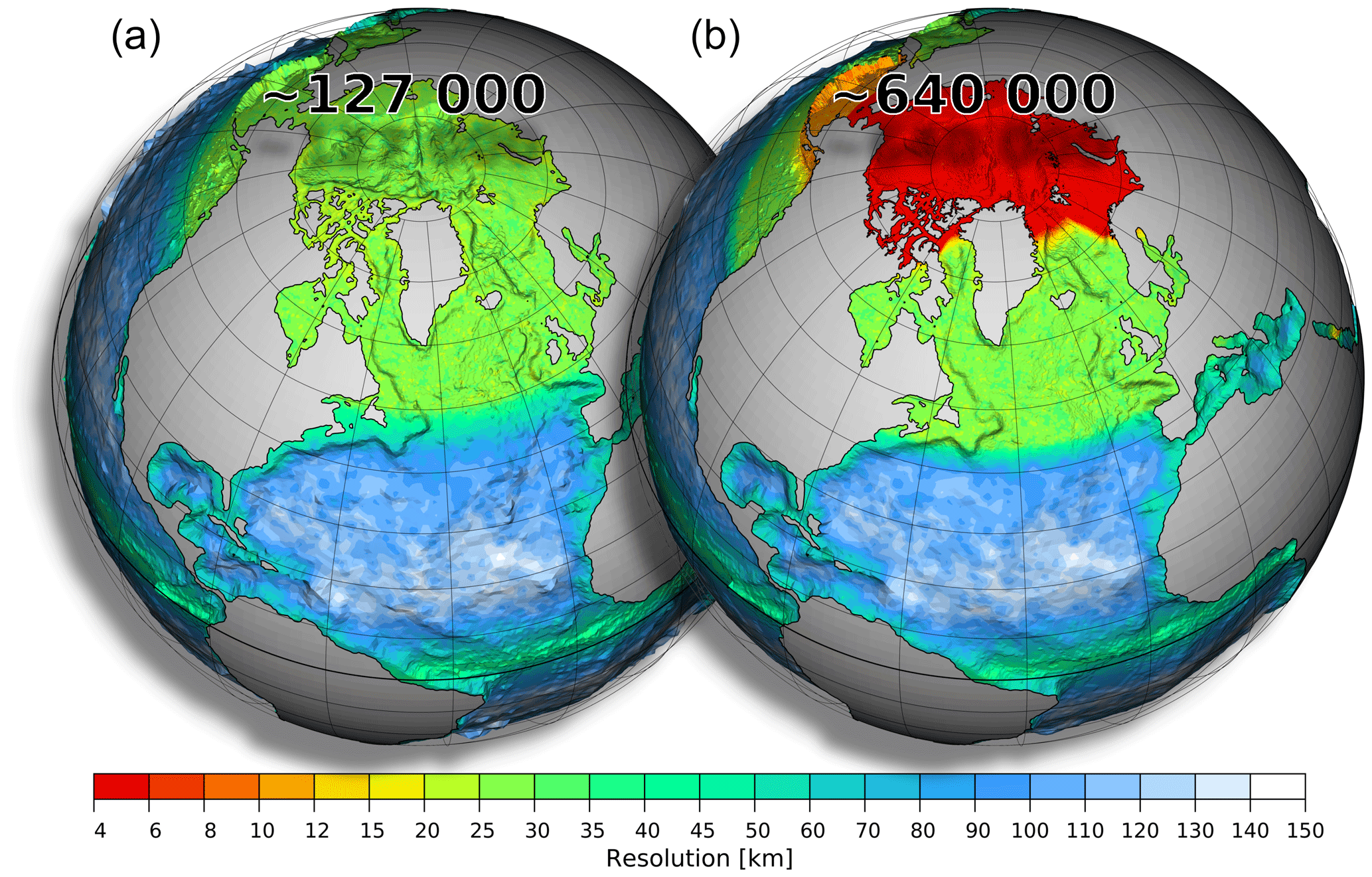
Figure 1 Horizontal resolution of mesh configurations used in this study: smaller reference (a, ∼ 127 000 surface vertices) and larger medium-sized (b, ∼ 640 000 surface vertices) meshes. The two meshes have the same resolution (nominal resolution of 1^∘ in most parts of the global ocean, ∼ 25 km north of 50^∘ N, ∼ 1/3^∘ at the Equator) except for the Arctic Ocean and Bering Sea. There, the medium-sized mesh has an increased resolution of 4.5 km and 10 km for the Arctic Ocean and Bering Sea, respectively.

2 Model configurations

For the general evaluation of FESOM2.0 and the comparison between FESOM1.4 and FESOM2.0, we use a relatively coarse resolution reference mesh consisting of ∼ 0.13 M surface vertices (Fig. 1a). The mesh has a nominal resolution (given by the mean side length of a triangle) of 1^∘ in most parts of the global ocean, except north of 50^∘ N, where resolution is set to ∼ 25 km, and in the equatorial belt, where resolution is increased to 1∕3^∘. The resolution in the coastal regions is also slightly increased. The mesh has 48 unevenly distributed layers, with a top layer of 5 m, increasing stepwise to 250 m towards the bottom. The same mesh has already been used in a variety of studies carried out with FESOM1.4, such as in the model intercomparison project of the Coordinated Ocean Ice Reference Experiment – phase II (CORE2), which proved that FESOM1.4 performs well compared to structured-mesh ocean models (see, e.g., Wang et al., 2016c, and other papers of the same virtual issue).

The computational performance and scaling estimates of FESOM2.0 and FESOM1.4 in Sect. 4 are conducted on a medium-sized mesh (Fig. 1b, 0.64 M surface vertices) that shares the same resolution with the reference mesh, except for the Arctic Ocean (including the Arctic gateways) and Bering Sea, where the resolution is refined to ∼ 4.5 and ∼ 10 km, respectively. All model setups are initialized with the Polar Science Center Hydrographic winter Climatology (PHC3.0, updated from Steele et al., 2001) and forced by the CORE interannually varying atmospheric forcing fields (Large and Yeager, 2008) for the period of 1948–2009.

3 Model elements: options and sensitivity studies

3.1 Linear free-surface and full free-surface formulations

FESOM1.4 supports two options for the free-surface formulation. One option is the linear free surface whereby the sea surface height equation is solved assuming a fixed mesh for tracer and momentum, and consequently tracers cannot be diluted or concentrated by ocean volume changes. With this option, to account for the impact of surface freshwater fluxes on salinity, a virtual salt flux is added to the salinity equation through the surface boundary condition. Although the formulation of a virtual salt flux mimics the effects of surface freshwater flux on the surface salinity, it has the potential to change local salinity with certain biases and affect model integrity on long timescales (Wang et al., 2014). This leads to the fact that modern ocean climate models, like the ones used in Danabasoglu et al. (2014), tend to abandon the fixed volume formulation in favor of a full free-surface formalism. This option was also implemented in FESOM1.4 but not widely used. The full free-surface formulation in FESOM1.4 uses the ALE framework in a finite-element sense where, due to costly updates of matrices and derivatives, only the surface grid points are allowed to move (Wang et al., 2014).

The ALE vertical coordinate formulation is also used in FESOM2.0 but in a finite-volume sense (see Donea and Huerta, 2003; Ringler et al., 2013; Adcroft and Hallberg, 2006; Danilov et al., 2017). It ensures a similar functionality between FESOM1.4 and FESOM2.0 with respect to geopotential and terrain-following coordinates and linear and full free-surface formulations. In FESOM2.0, the ALE formalism became an essential and elementary integrated part of the numerical core, unlike in FESOM1.4, where it was only an additional feature to allow the surface to move in the full free-surface formulation. FESOM2.0 also offers the possibility to move all vertical layers, later referred to as zstar (Adcroft and Campin, 2004), which becomes a more frequently used option, since the associated computational cost in FESOM2.0 is strongly reduced compared to FESOM1.4.

The adaptations that are made to the numerical code of FESOM2.0 in the course of the ALE implementation are discussed in detail in Danilov et al. (2017). The main part of the ALE implementation is to introduce the thickness of model ocean layers as an additional 3-D variable that is allowed to vary in space and time. Thus, the ALE approach in FESOM2.0 not only allows one to relatively easily implement different vertical discretizations by manually assigning different initial layer thicknesses but also supports time-varying vertical grids, including the full nonlinear free surface and meshes following isopycnals. This means that the vertical grid can be fully Eulerian, fully Lagrangian or something in between (see also Petersen et al., 2015).

For the linear free-surface (hereafter called linfs) option in FESOM2.0, the 3-D layer thicknesses are fixed in time and the bottom-to-top volume of each vertical grid cell is kept constant during the simulation. This requires, like in FESOM1.4, the introduction of a virtual salinity flux as an additional surface boundary condition in the salinity equation to account for changes in salinity through surface freshwater fluxes (rain, evaporation, river runoff, freshwater fluxes from ice melting/freezing).

In the full nonlinear free-surface option, the total water column thickness is allowed to vary over time following the change in sea surface height (SSH). Freshwater fluxes can be directly applied to the surface layer thicknesses of the thickness equation, which then modifies the surface salinity by changing the volume of the upper grid cells. The ocean heat content change associated with surface water fluxes is added to the ocean temperature equation as the surface boundary condition. For the full free-surface case in FESOM2.0, we distinguish between two options. The first one is called zlevel, where only the thickness of the surface layer is varied following the change of SSH, while all other layers are kept fixed (Adcroft and Campin, 2004; Petersen et al., 2015; Danilov et al., 2017). This is equivalent to the only full free-surface option available in FESOM1.4. The second option is zstar, where the total change in SSH is distributed equally over all layers, except the layer that touches the bottom. This allows all layers above the bottom layer to move vertically with time. In this case, each layer only moves by a fraction of the total change of water column thickness. With the zlevel option, the upper layer thickness can be altered more than with the zstar case, so it is recommended to use zstar in the full free-surface formulation for the sake of stability.

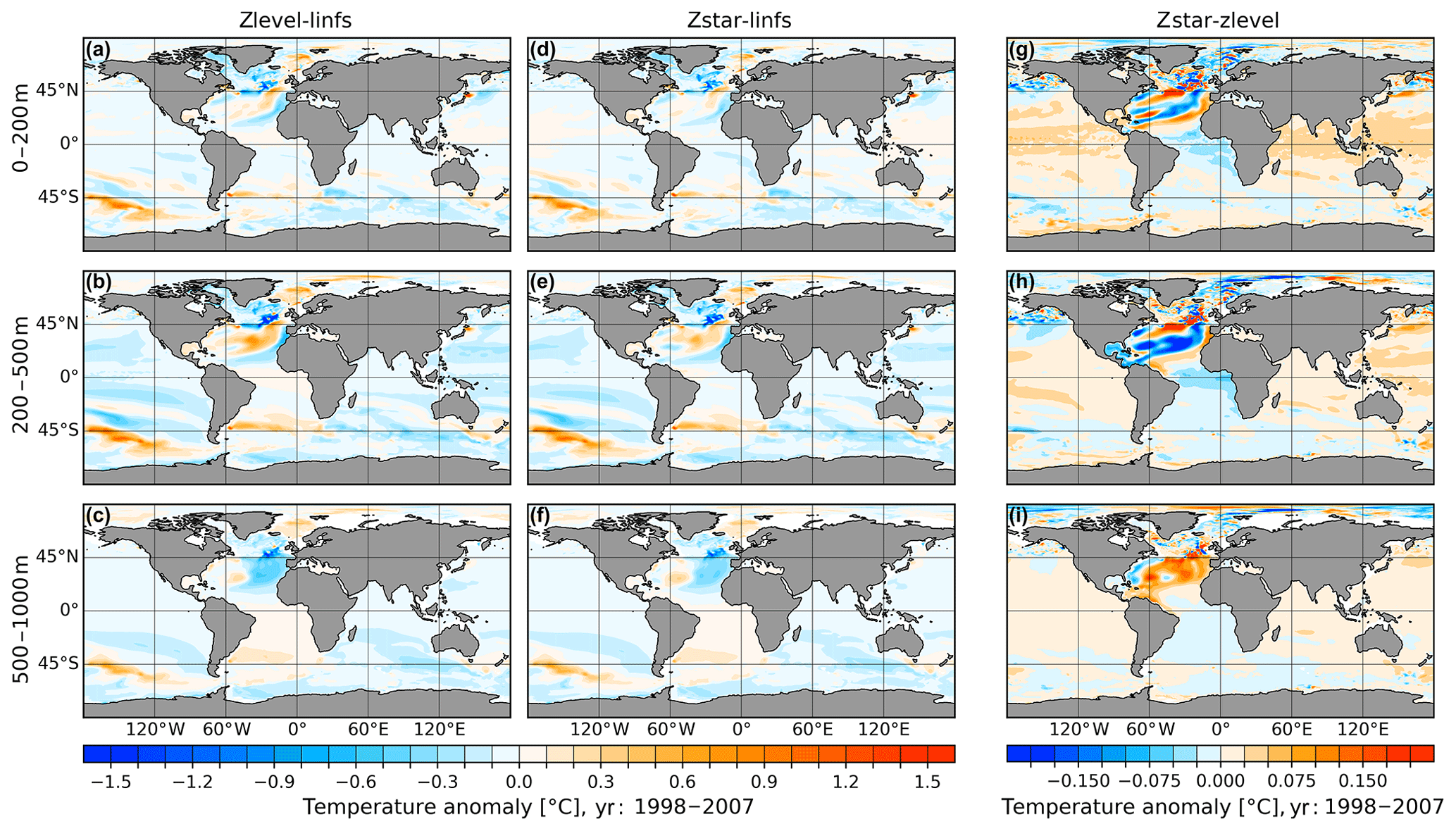
Figure 2 Temperature anomalies of the full free-surface simulations with respect to the linear free-surface simulation: zlevel minus linfs (a–c) and zstar minus linfs (d–f). Panels (g–i) show the temperature difference between the two full free-surface simulations (zstar minus zlevel). From top to bottom, the three rows show the results for three different depth ranges: 0–200, 200–500 and 500–1000 m. Averages over the time period of 1998–2007 are shown. Note that different color scales are used.

Figure 3 Same as Fig. 2 but for salinity.

In order to understand the effect of the linear free-surface and the two full free-surface options on the simulated ocean state, three model simulations were conducted using the linfs, zlevel and zstar configurations. Figure 2 compares the temperature anomalies of zlevel and zstar with respect to linfs (first and second columns) and the temperature difference between zlevel and zstar (third column, zstar minus zlevel) over three different depth ranges. All presented model results are averaged over the same time period of 1998–2007 as in Danilov et al. (2017) to emphasize the improvements that have been achieved and to keep the here-presented results qualitatively comparable to the results shown there.

The overall patterns of temperature anomalies of zlevel and zstar with respect to linfs are very similar for all three depth ranges, since the difference between zlevel and zstar is smaller by nearly 1 order of magnitude. Compared to linfs, both zlevel and zstar show a strong cooling signal along the pathway of the North Atlantic Current (NAC), Irminger Current (IC) as well as the Canary Current (CC) and Atlantic Northern Equatorial Current (NEC) that reaches from the surface to the depth range of 500–1000. The surface and intermediate depth range shows positive temperature anomalies in the center of the subtropical gyre, Greenland–Iceland–Norwegian (GIN) seas and western Southern Ocean (SO). The deep depth range is dominated by a cooling anomaly in the eastern North Atlantic. The direct comparison between zlevel and zstar (Fig. 2, third column) shows that the zstar in the surface and intermediate depth ranges is around 0.2 ^∘C warmer along the path way of the NAC, CC and NEC but colder by up to −0.2 ^∘C in the GIN seas, Arctic Ocean (AO), central North Atlantic (NA) and northeastern Pacific. In the depth range of 500–1000 m, zstar shows a warming of up to 0.15 ^∘C in the central NA accompanied by colder anomalies along the pathway of the deep western boundary current and AO. Overall, the temperature difference between the two full free-surface cases is much smaller than that caused by using the linear free surface.

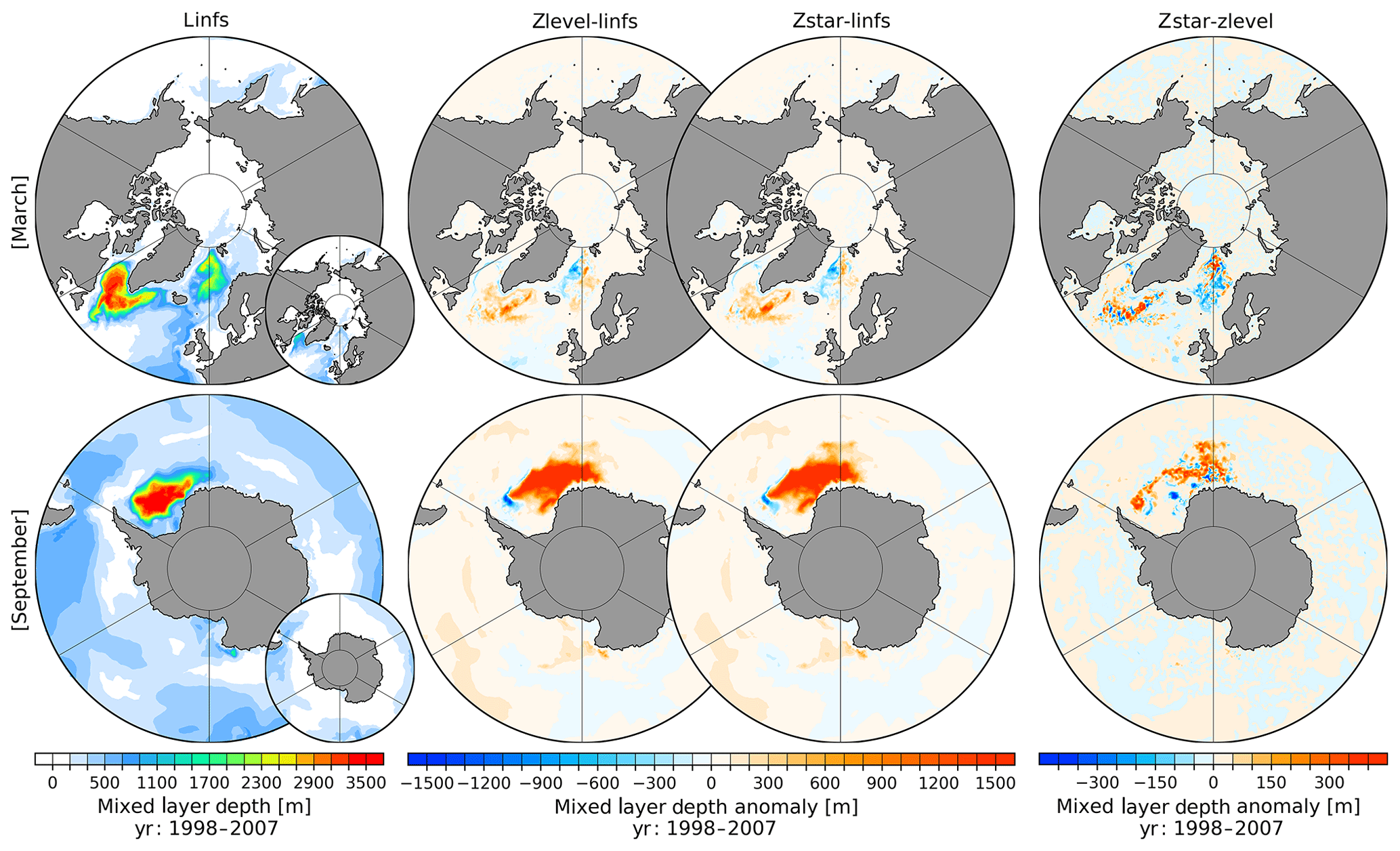
Figure 4 March (upper row) and September (lower row) mixed layer depth after the definition of Monterey and Levitus (1997, MLD1) for the linear free-surface case (linfs, first column) averaged for the time interval of 1998–2007. The second and third columns show the anomalous MLD1 for the full free-surface modes zlevel (second column) and zstar (third column) with respect to the linfs mode. The fourth column presents the anomalous MLD1 between the two full free-surface modes (zstar minus zlevel). The small inset plot shows the mixed layer depth after the definition of Large et al. (1997, MLD2).

Figure 3 presents the same comparison as Fig. 2 but for salinity. The salinity of zlevel and zstar (Fig. 3, first and second columns) shows nearly the same anomalies with respect to linfs. Both zlevel and zstar indicate a salinification of up to 0.2 psu in the surface depth range of the AO, while the intermediate and deep depth ranges show some freshening. All considered depth ranges of the Labrador Sea (LS), Irminger Sea (IS), part of the eastern NA as well as the surface depth range of the GIN seas show a freshening of up to −0.2 psu. The surface and intermediate depth ranges of zlevel and zstar in the central NA, South Atlantic (SA) as well as parts of the SO show slight positive salinity anomalies with respect to linfs. The direct comparison of the salinity between zlevel and zstar (zstar–zlevel; Fig. 3, third column) indicates slight differences for the surface and intermediate depth ranges of the AO as well as central NA. The same as for temperature, the difference in salinity between the two free-surface options is much smaller than the difference between any of these and the linear free-surface option.

In FESOM2.0, we tried two different ways of computing the mixed layer depth (MLD). One way follows the definition of Monterey and Levitus (1997), who compute MLD as the depth at which the density over depth differs by 0.125 sigma units from the surface density (Griffies et al., 2009). This MLD definition was also supported in FESOM1.4 (hereafter referred to as MLD1). The other way follows Large et al. (1997), who suggest to compute MLD as the shallowest depth where the vertical derivative of buoyancy is equal to a local critical buoyancy gradient (Griffies et al., 2009) (hereafter referred to as MLD2). Both definitions reveal large MLD differences especially in the Southern Ocean. The first column in Fig. 4 shows the northern hemispheric March (upper row) and southern hemispheric September (lower row) mean MLD averaged over the period of 1998–2007 in the linfs option. The main plots show the absolute and anomalous values of MLD1, while the small insets show the absolute values of MLD2. In the Northern Hemisphere, March MLD1 indicates mixed depths of up to 3400 m in the entire Labrador Sea, together with a weaker MLD1 in parts of Irminger Sea and central GIN seas, while MLD2 shows only a maximum of ∼ 1600 m in the northwest Labrador Sea with a weaker MLD of ∼ 900 m in the Irminger Sea and ∼ 450 m along the pathway of the Norwegian boundary current. The southern hemispheric September MLD1 (linfs) shows high values for the entire Weddell Sea, while MLD2 indicates no large values in the entire Southern Ocean.

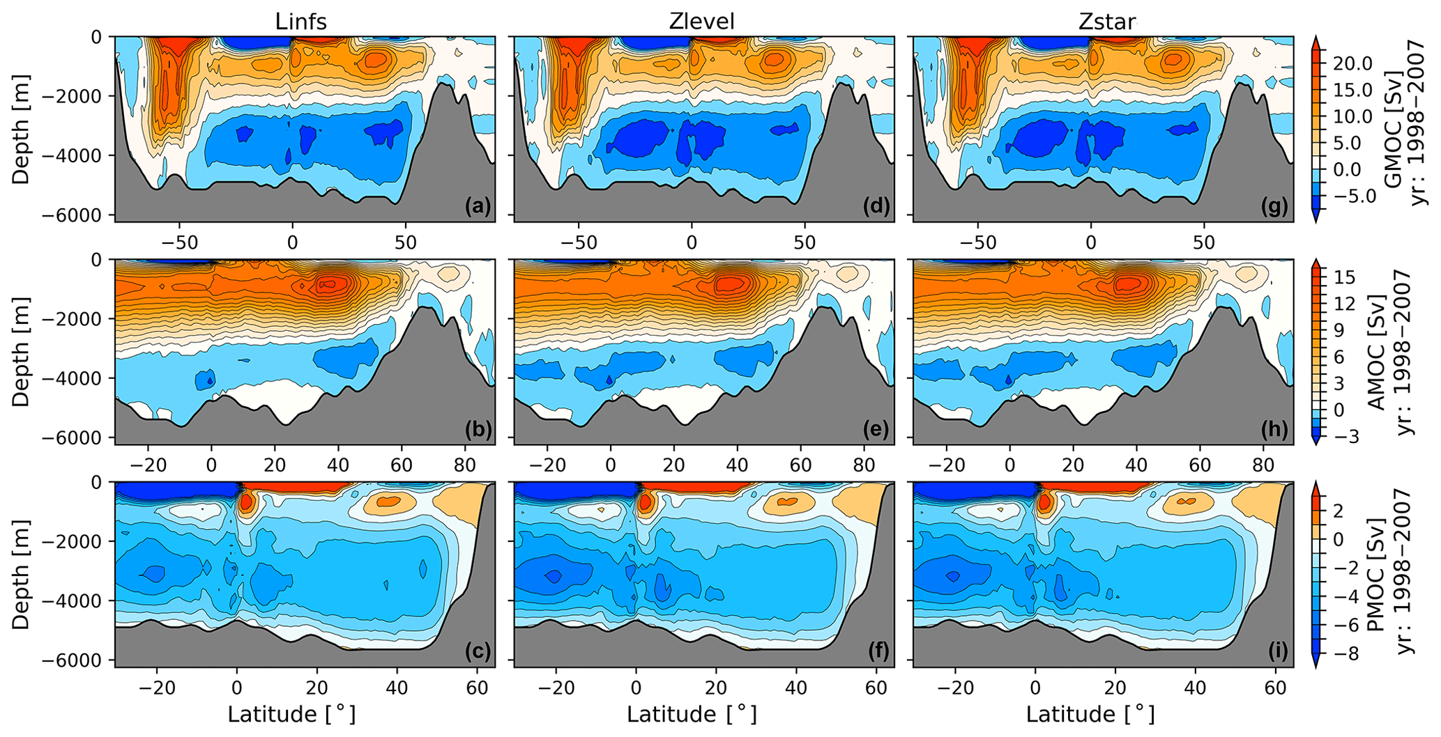
Figure 5 Global (GMOC, a, d, g), Atlantic (AMOC, b, e, h) and Indo-Pacific (PMOC, c, f, i) meridional overturning circulations for the linear free-surface formulation linfs (a–c) and the full free-surface zlevel option (d–f) and zstar option (g–i). The average over the time period of 1998–2007 is shown. Note that different color ranges are used.

The differences in MLD1 between zlevel and zstar with respect to linfs (Fig. 4, second and third columns) show almost identical patterns for March and September, with a gain of March MLD in the eastern LS, western IS and central GIN seas, accompanied by a reduction of MLD in the western GIN seas. The difference in September MLD1 between zlevel and zstar with respect to linfs, shows a strong gain in the MLD for the entire eastern Weddell Sea (WS) with a slight loss in MLD on its western side. The direct MLD comparison between zlevel and zstar (Fig. 4 fourth column, zstar minus zlevel) reveals a local heterogeneous anomaly pattern for March and September with a maximum amplitude of ∼ 300 m and with a tendency towards a slightly increased zstar March MLD in the LS and IS as well as a reduced MLD in the GIN seas, while the zstar September MLD reveals for the northern WS a general tendency towards a gain in MLD when compared to zlevel. Inspecting the spread in MLD patterns from these simulations, we conclude that (1) as a consequence of different stratification strength the MLD map is sensitive to the way of how it is computed. The largest discrepancies between two diagnostics used in this paper are in the SO. (2) Through altering the stratification, different model options can affect various MLD diagnostics in different ways.

To demonstrate the effect of the linear free surface and full free surface on large-scale ocean circulation, we show the streamfunction of the meridional overturning circulation (MOC) for the global (GMOC, upper row), Atlantic (AMOC, middle row) and Indo-Pacific meridional overturning circulations (PMOC, lower row) in Fig. 5 for the three simulations. The MOC contains the contribution from the Eulerian and eddy-induced circulation (bolus velocity). All three cases show similar shapes of the North Atlantic deep water (NADW) upper circulation cell as well as Antarctic Bottom Water (AABW) cell of the GMOC, AMOC and PMOC but with slight differences in their circulation strength. For the GMOC, linfs obtains a stronger NADW upper circulation cell with maximum transport of ∼ 16 Sv at ∼ 40^∘ N, while zlevel and zstar have a slightly weaker maximum transport of ∼ 15 Sv at 40^∘ N. The GMOC AABW cell in linfs reveals that north of 40^∘ N there is 0.2 Sv stronger transport and south of 0^∘ up to 2.0 Sv weaker transport when compared to zlevel and zstar. The strength and structure of the Southern Ocean Deacon cell (Kuhlbrodt et al., 2007) look fairly the same for all three cases. All three simulations show no connection of the AABW cell to the upper circumpolar deep water (UCDW).

The NADW cell of the AMOC has a maximum strength of 15 and 14 Sv for linfs and the two full free-surface cases, respectively. For the AABW cell of the AMOC, the three simulations have similar strength and shape. The shape of the PMOC bottom cell is fairly the same for all three simulations. However, the PMOC in linfs shows an up to 1 Sv weaker AABW south of 0^∘ accompanied by a 0.3 Sv stronger PMOC north of 40^∘ N. For all the three diagnosed meridional overturning circulation streamfunctions (GMOC, AMOC and PMOC), the two full free-surface cases show negligible difference.

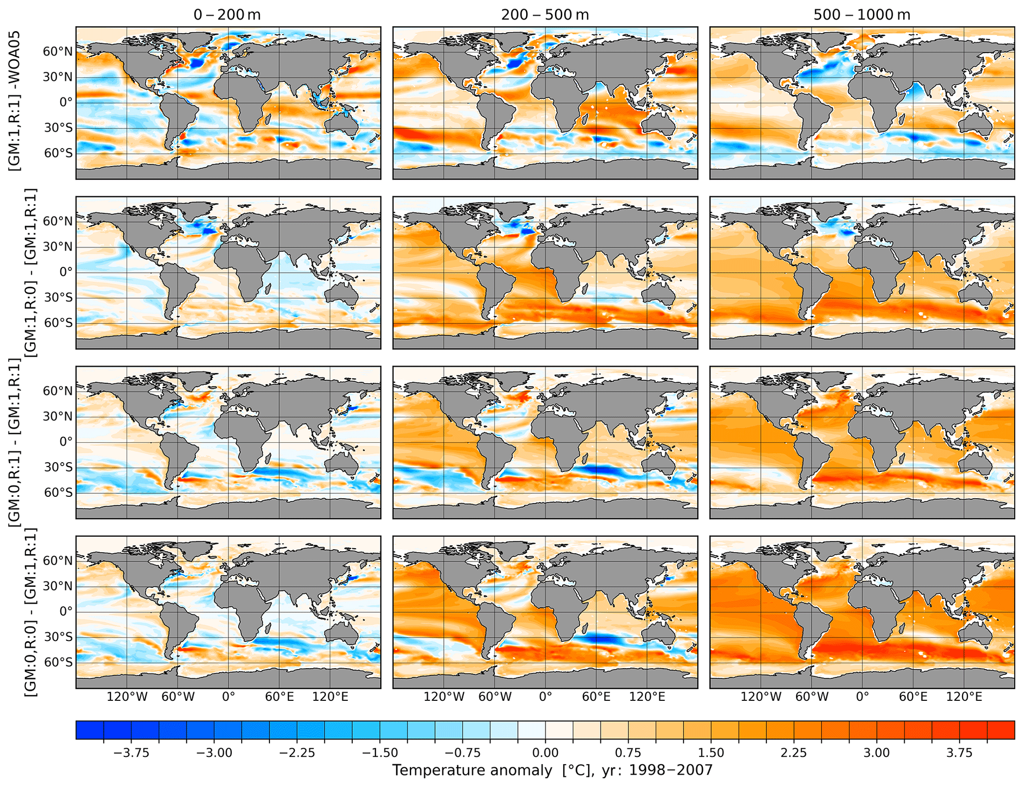
Figure 6 First row: temperature biases in the reference simulation with respect to the World Ocean Atlas 2005 (WOA05; Locarnini et al., 2006; Antonov et al., 2006) climatology for three different depth ranges: 0–200 m (left), 200–500 m (middle) and 500–1000 m (right). In the reference simulation, both the GM and Redi diffusion parameterizations are switched on (:1). Another three rows show the temperature differences between sensitivity runs and the reference run. The second row shows the impact when only the Redi diffusivity is switched off (:0), the third row when only GM is switched off and the fourth row when both of them are switched off. The average over the period of 1998–2007 is shown.

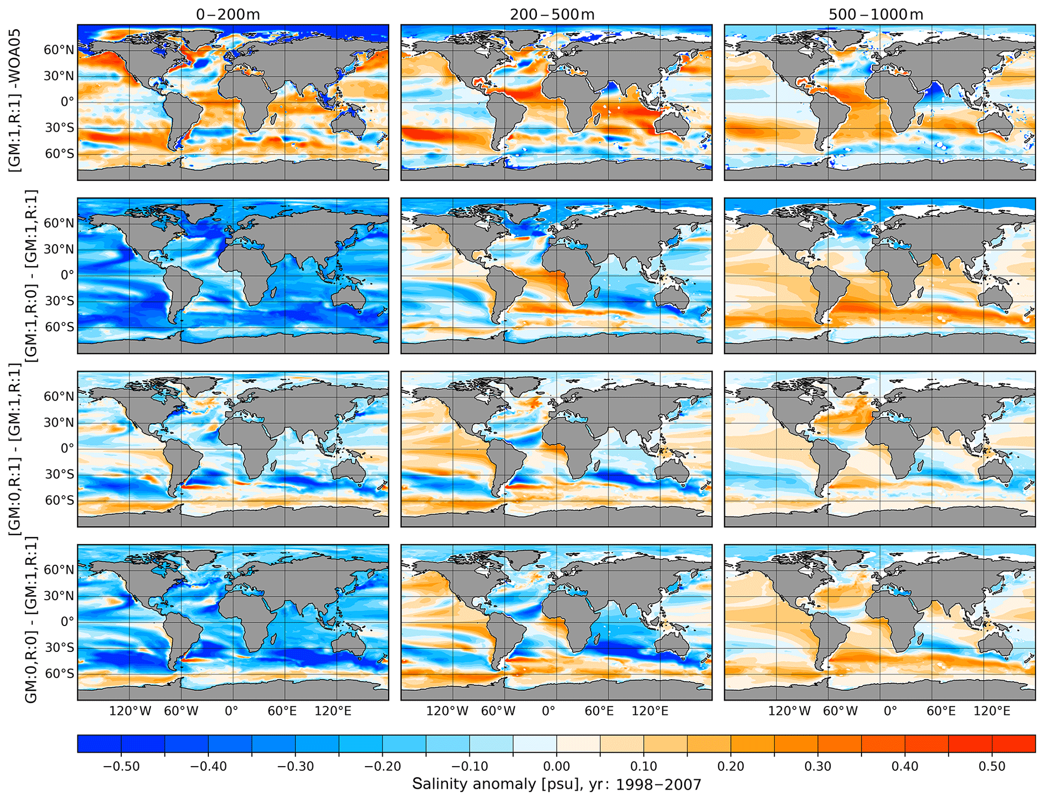
Figure 7 Same as Fig. 6 but for salinity.

Overall, the sensitivity tests indicate that the differences in ocean hydrography and circulation caused by using linear free-surface and full free-surface options are not negligible. However, the differences are less significant than those between different ocean models in the CORE-II model intercomparison project (e.g., Danabasoglu et al., 2014) and also less significant than the differences associated with tuning other model parameters as presented in the following subsections.

3.2 Parameterizations of eddy stirring and mixing

With the increase of computational resources, the ocean modeling community aims at resolving the mesoscale eddies in the ocean by increasing resolution of computational grids. As discussed in Hallberg (2013), the resolution of two grid points per Rossby radius of deformation should be the target in the near future. Considering that the Rossby radius can be as small as a few kilometers in high latitudes and even less than 1 km in high-latitude shelf regions, the size of the computational grid needed to resolve mesoscales globally is far larger than those which are currently employed in climate models. Moreover, there are indications that in some regions the threshold of two grid points per Rossby radius marks only the lower boundary of the desired grid resolution (Sein et al., 2017). Therefore, parameterizations for mesoscales are still required in state-of-the-art ocean models. In this section, we analyze how the Gent–McWilliams (GM) parameterization of eddy stirring (Gent and McWilliams, 1990; Gent et al., 1995) and the Redi isoneutral diffusion (Redi, 1982) of tracers impact the simulated ocean state.

The implementation of GM in FESOM2.0 (see Danilov et al., 2017, for more details) follows the algorithm proposed by Ferrari et al. (2010). It operates with explicitly defined eddy-induced velocity, which is different from that employed in FESOM1.4, where the skewness formulation of Griffies et al. (1998) is used. The scheme employed in FESOM2.0 allows for natural tapering through the vertical elliptic operator and does not require an extra diagnostic of eddy-induced velocities which are, in contrast to FESOM1.4, explicitly defined. All specifications applicable to the GM parameterization in FESOM1.4 have been ported to FESOM2.0. In the default model configuration, the thickness diffusivity coefficient is scaled vertically (see Ferreira et al., 2005; Wang et al., 2014) and also varies with horizontal resolution. The maximum thickness diffusivity is set to 2000 m² s⁻¹ and is gradually switched off starting from a resolution of 40 km until 30 km using a linear function. The Redi isoneutral diffusion is set equal to the thickness diffusivity following the tuning experience gained with FESOM1.4. In order to verify the related model code and understand the effects of the GM and isoneutral diffusion parameterizations newly implemented in FESOM2.0, we conducted four experiments where we sequentially switch these parameterizations on and off.

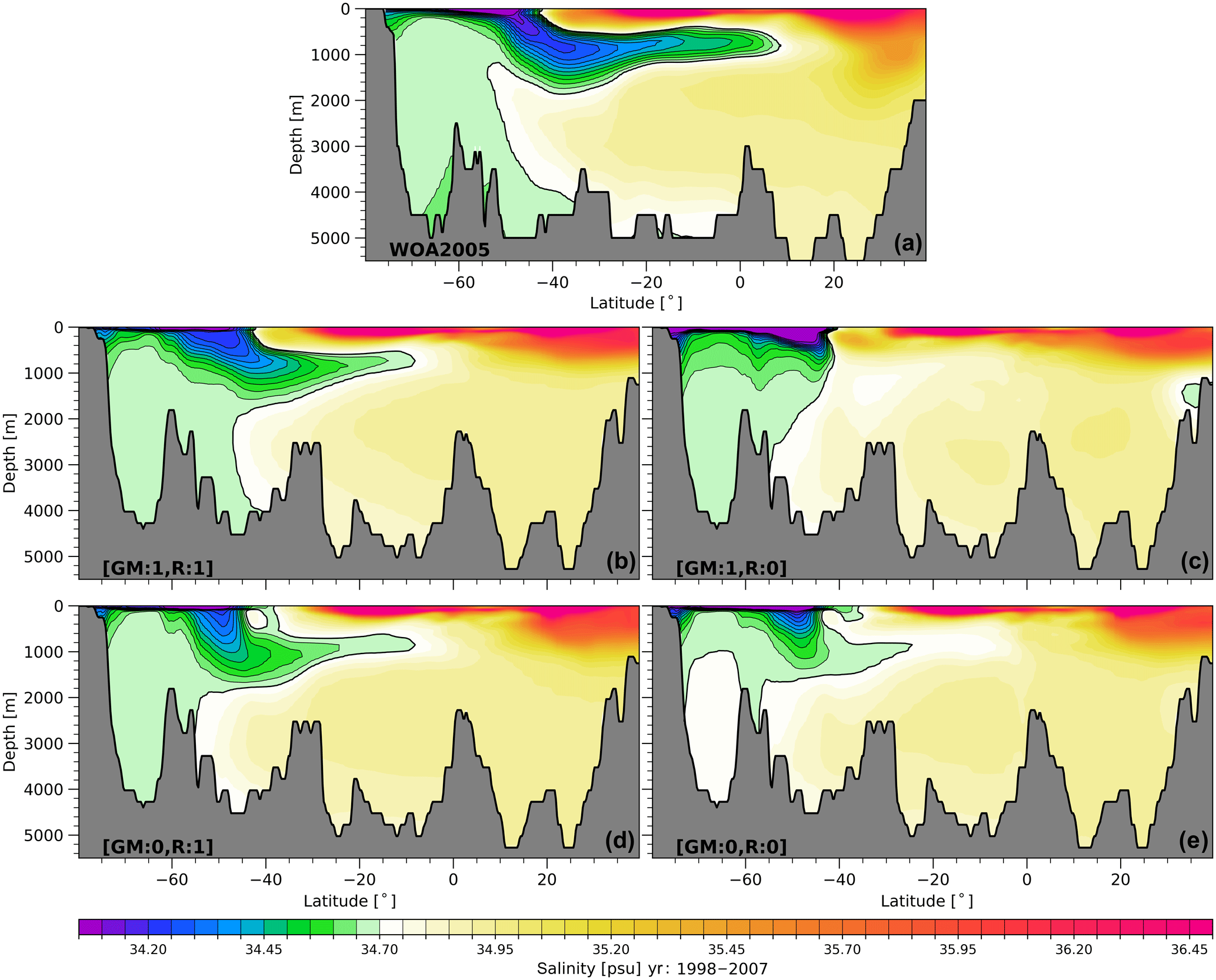
Figure 8 (a) Mean salinity in a vertical section from −80^∘ S, −30^∘ W, to 40^∘ N, −30^∘ W, derived from WOA05 (Locarnini et al., 2006; Antonov et al., 2006) annual climatology. The other four panels show the results from model simulations: (b) the reference run with switched on GM and Redi, (c) the run with Redi diffusivity set to zero, (d) the run with GM switched off and (f) both parameterizations switched off. Contour lines highlight the spreading of Antarctic Intermediate Water (< 34.70 psu) northward.

3.2.1 Changes in hydrography

In the reference simulation, we applied both the GM and Redi diffusion parameterizations. Then three sensitivity simulations were carried out. In the first one, we set the Redi diffusivity to zero; in the second, we zeroed the GM stirring coefficient; and in the third one, we switched off both parameterizations. The simulated temperature and salinity biases for the reference run and the differences between sensitivity and the reference simulations are shown in Figs. 6 and 7. Without Redi diffusivity, the modification of T and S within the same density classes can only be realized via the vertical turbulent closure or through the spurious mixing of the advection scheme (there is no explicit horizontal diffusion in FESOM2.0). In this case, there is no consistent way for the model to mix the water properties along isopycnals. Hence, it is not surprising that the absence of isoneutral mixing results in the overall fresher upper ocean in response to reduced mixing of salt between the deep and upper oceans. It is particularly visible in patterns of horizontal anomaly in the subpolar North Atlantic (SNA) and in the vicinity of the convection zones. In the Southern Ocean (SO), the change in position of the isopycnal slope is visualized in Fig. 8 via the meridional salinity section across 30^∘ W as practiced in previous climate studies (see, e.g., Armour et al., 2016). Although the slope of the Antarctic Intermediate Water (AAIW) in the SO is predominantly determined by the interplay between Ekman pumping and eddy transport, isoneutral diffusion shows pronounced impacts on the representation of water mass distribution. Without isoneutral diffusion, the subsurface AAIW becomes more saline, while excessive freshwater accumulates within the upper 500 m. The increased presence of the freshwater in the upper ocean strengthens the halocline and prevents the deep water production. Indeed, the corresponding reduction of MLD is shown in Fig. 9. Opposite to the upper ocean, except in the SNA, the deep ocean shows the overall increase in salinity simply as a consequence of the total salt conservation in these experiments (Fig. 7). As one might expect, the corresponding temperature change in the deep ocean in terms of buoyancy is opposite to that in salinity.

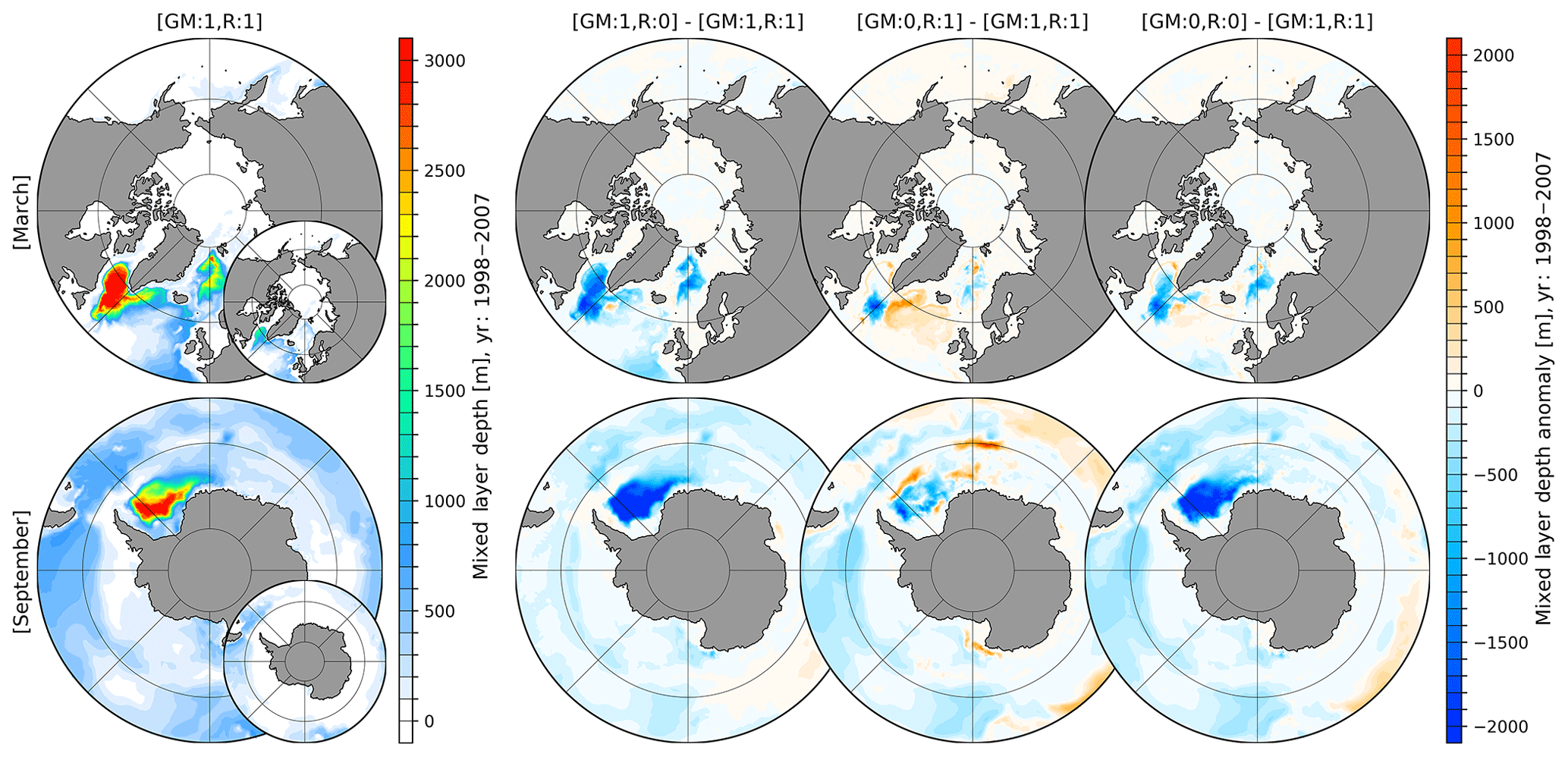
Figure 9 First column: March (upper row) and September (lower row) mean mixed layer depth (MLD, definition after Monterey and Levitus, 1997) for the simulation with switched on (:1) Gent–McWilliams (GM) parameterization and Redi (R) diffusion averaged over the period of 1998–2007. Second to fourth columns: anomalous MLD of simulations with either switched off (:0) GM or R, or both switched off with respect to the control simulation where GM and R are both switched on. The small inset plots show the MLD after the definition of Large et al. (1997).

In the experiment without the GM parameterization, the isopycnal slope induced by the winds along the main oceanic fronts increases until it becomes unphysically balanced by processes like diffusion and numerical mixing. In the absence of bolus overturning, the Deacon cell circulation in the SO is strengthened in this experiment, with stronger downwelling on the northern side of the Antarctic Circumpolar Current (ACC) and stronger upwelling on the southern side (see Sect. 3.2.2). As a consequence, the temperature and salinity show negative and positive anomalies on the northern and southern sides of the ACC, respectively. Although sharper isopycnal slopes are expected to support deep convection, the MLD in this experiment did not change much as compared to the reference configuration (see Fig. 9). Indeed, in contrast to the no-Redi experiment, the simulated slope of the AAIW isohalines in the SO becomes unrealistically steep. As a result, the surface freshwater penetrates along steep isopycnals to a deeper depth than in the reference experiment. We conclude that a delicate interplay between GM and Redi parameterizations is required in order to properly simulate the hydrographic properties in the global ocean using non-eddy-revolving numerical grids.

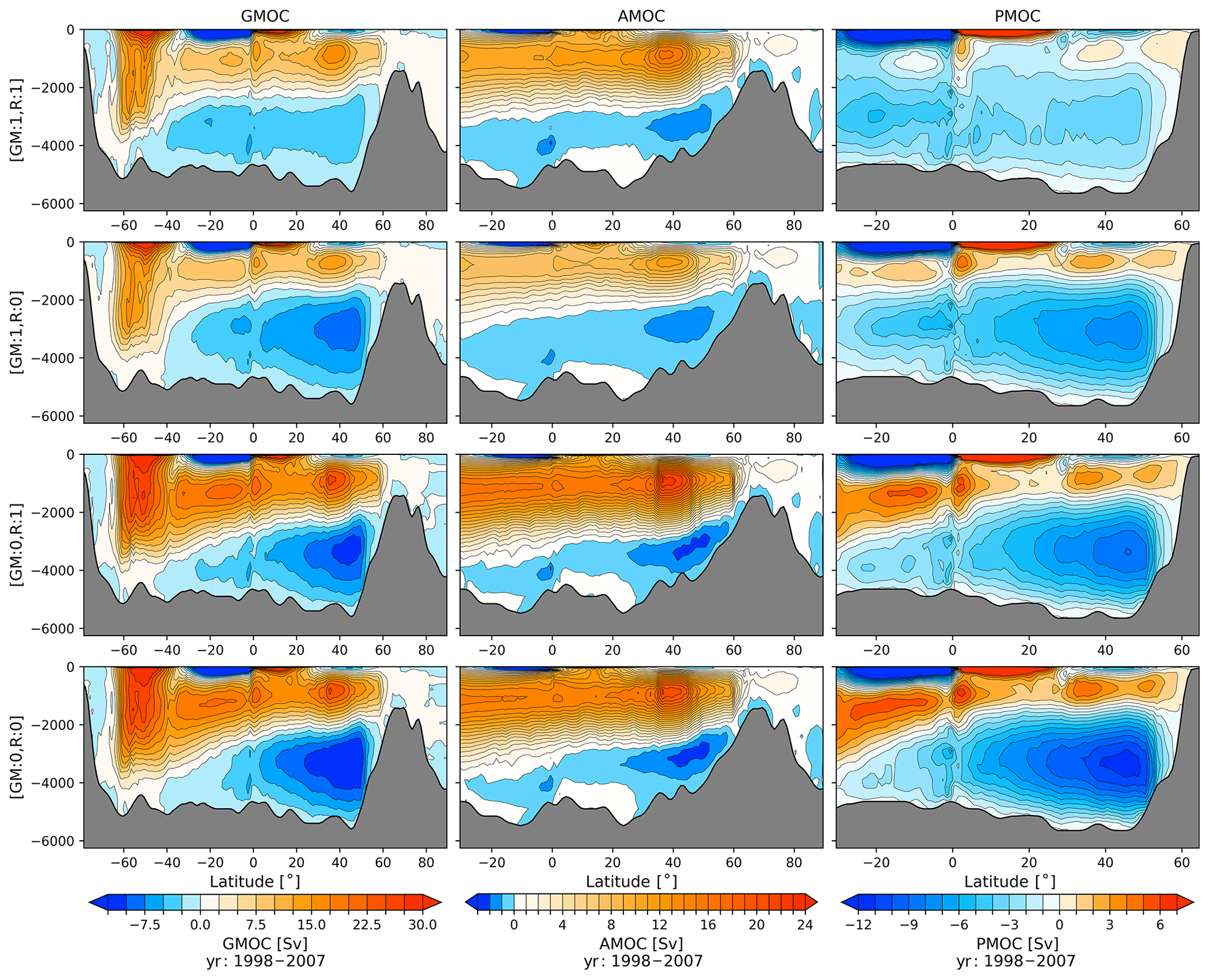
Figure 10 GMOC (first column), AMOC (second column) and PMOC (third column) averaged for the time period of 1998–2007 for (first row) the reference run with switched on GM and Redi (:1), (second row) the run with switched off Redi diffusivity (:0), (third row) GM switched off and (fourth row) both parameterizations switched off. Note different color ranges are used.

3.2.2 Changes in thermohaline circulation

The influence of GM and Redi parameterizations on the thermohaline circulation is illustrated by the MOC (Fig. 10). In runs without GM, it is computed using only Eulerian velocities. In runs using GM, MOC contains both the Eulerian and eddy-induced velocities. The latter ones are also shown separately in Fig. S1. For the reference run, the MOC streamfunction is plotted in the upper panels of Fig. 10. The upper cell originates primarily from the Atlantic Ocean with the maximum located at ∼ 1000 m depth. The maximum value is ∼ 15 Sv at 40^∘ N. The bottom cell for the AABW is contributed from both Atlantic and Pacific oceans and is also well reproduced with the maximum strength of ∼ 5 Sv.

The run with Redi diffusivity set to zero and switched on GM is characterized by the smallest AMOC among the sensitivity experiments. In contrast, the run without GM is characterized by the largest AMOC. This is also expected since without GM the isopycnal slopes become steeper and induce stronger boundary currents accompanied by stronger return flows at depths. The behavior aligns with findings by Marshall et al. (2017): the bottom cell in the Atlantic Ocean, which indicates the spread of the AABW, is larger in runs with GM. Interestingly, the bottom MOC cell for the global ocean is increased in all sensitivity experiments compared to the reference run. As shown in Fig. 10, this is primarily due to the contribution from the Pacific Ocean. Furthermore, it shows an extremum at ∼ 40^∘ N which is absent in the reference simulation.

3.3 Diapycnal mixing

Mixing across density surfaces is an essential part of the thermohaline circulation. It can control not only the circulation and heat budget of the global ocean but also the distribution of nutrients and biological agents in the ocean (Wunsch and Ferrari, 2004; De Lavergne et al., 2016). Therefore, a proper representation of diapycnal mixing in ocean models is essential. Mixing processes are not resolved in ocean models and have to be parameterized. Current climate models are often utilized with the Pacanowski and Philander (1981, hereafter referred to as PP) or the K-profile parameterization (KPP; Large et al., 1994) vertical mixing schemes, depending on the physical complexity they address. Both mixing schemes are implemented in FESOM2.0. During the tuning and parameter-testing phase, and based on our experience with FESOM1.4, we slightly modified both mixing schemes compared to the original implementation of Pacanowski and Philander (1981) and Large et al. (1994), by adjusting the background vertical diffusivity and adding vertical mixing depending on the diagnostically computed Monin–Obukhov length, to overcome certain biases especially in the Arctic region and Southern Ocean.

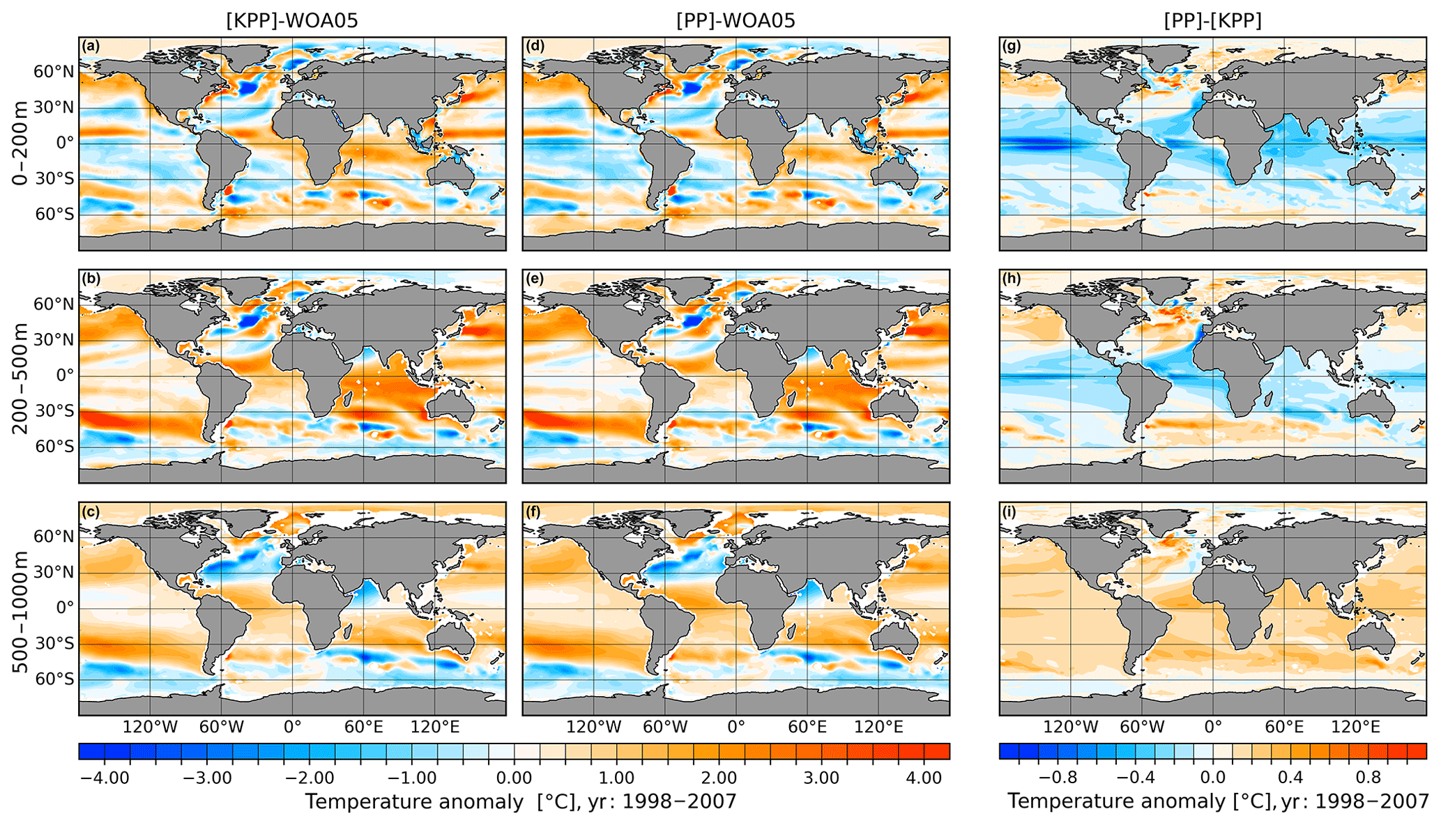
Figure 11 Temperature biases in model simulations referenced to WOA05 (Locarnini et al., 2006; Antonov et al., 2006) averaged over the period of 1998–2007 for (a–c) the simulation with the KPP vertical mixing scheme and (d–f) the simulation with the PP mixing scheme. Panels (g–i) show the difference between the two simulations. From top to bottom, the panels show the vertically averaged fields for the depth ranges of 0–200 m (a, d, g), 200–500 m (b, e, h) and 500–1000 m (c, f, i).

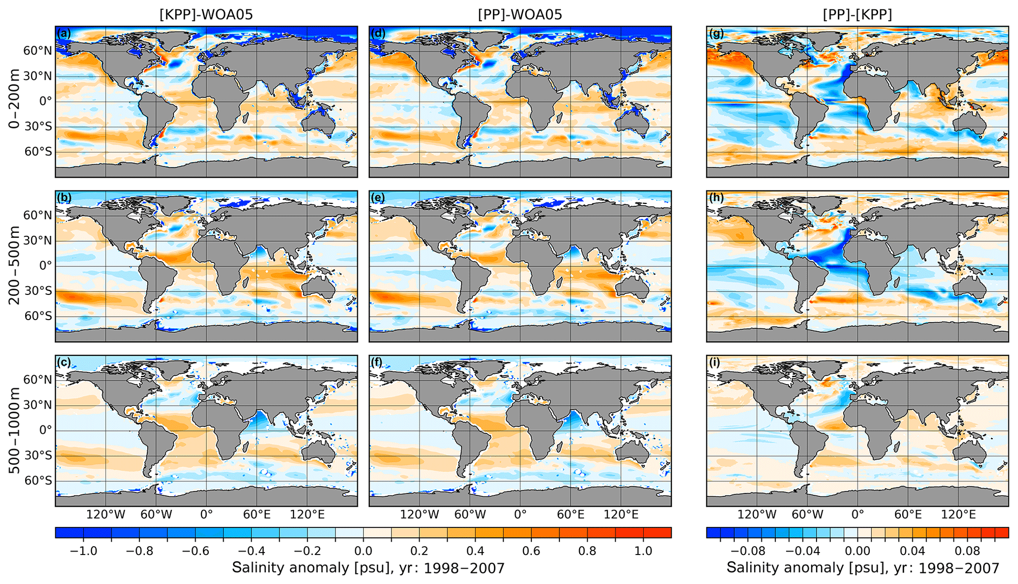
Figure 12 Same as Fig. 11 but for salinity.

The PP scheme used in FESOM2.0 computes the subgrid-scale turbulent vertical kinematic flux of tracer and momentum via the local Richardson number (Ri). The vertical background viscosity for momentum is set to 10⁻⁴ m² s⁻¹. For potential temperature and salinity, we deviate from the standard PP implementation and use a non-constant, depth- and latitude-dependent background diffusivity with values between 10⁻⁴ and 10⁻⁶ m² s⁻¹ (see Fig. S3). The original PP scheme, as well as the PP scheme used in FESOM1.4, used a constant background diffusivity here. For the convection case (Ri < 0), vertical diffusivity and viscosity are set to 0.1 m² s⁻¹ in order to remove static instability to ensure stable density profiles.

The original PP scheme is further augmented by the mixing scheme proposed by Timmermann et al. (2004). In this scheme, the vertical mixing within the diagnostically computed Monin–Obukhov length, which depends on surface friction velocity, the sea ice drift velocity and surface buoyancy flux, is increased to a value of 0.01 m² s⁻¹ to further stir the seasonal varying wind-mixed layer depth. This strongly reduced the hydrography biases, especially in the Southern Ocean (not shown).

In contrast to the PP scheme, the KPP scheme explicitly calculates diffusivity throughout the boundary layer and provides a smooth transition to the interior diffusivity. Within the boundary layer, scalar fields (temperature and salinity) obtain a counter-gradient transport term, provided that the net surface buoyancy forcing flux is unstable. In the current version of FESOM2.0, the background diffusivity in KPP uses the same non-constant latitude- and depth-dependent background diffusivities as in PP. Maximum diffusivity and viscosity due to shear instability are set to be $\mathrm{5.0}\times {\mathrm{10}}^{-\mathrm{2}}$ and $\mathrm{5.0}\times {\mathrm{10}}^{-\mathrm{3}}$, respectively. The magnitude of the tracer diffusivities is reduced by 1 order of magnitude between the equatorial belt of 5^∘ S and 5^∘ N following the observations of Gregg et al. (2003). Also, the KPP scheme is augmented by the same mixing scheme proposed by Timmermann et al. (2003) and that is used in PP.

In order to show the sensitivity to the choice of the vertical mixing schemes, two simulations with different vertical mixing schemes are conducted. The depth-integrated model biases of the surface, mid-ocean and deep ocean are shown for temperature and salinity in Figs. 11 and 12, respectively. Compared to WOA05, the KPP simulation generally overestimates ocean temperatures in the surface layers in the Kuroshio region, equatorial belt, Indian Ocean and Southern Ocean, and underestimates them in the subtropics and North Atlantic subpolar gyre region. In the mid-ocean and deep ocean, temperature is generally overestimated, except for the ACC and the North Atlantic.

Figure 13 March (a, b) and September (c, d) MLD for the simulation with KPP (a, c) and PP (b, d) vertical mixing averaged over the period of 1998–2007. Small inset plots show the MLD after the definition of Large et al. (1997).

Differences between PP and KPP experiments are very small in the open ocean, compared to the model bias with respect to WOA05. The largest differences in the surface layers occur in the equatorial Pacific, where temperature simulated with PP is colder than in the case of KPP. In the deep ocean, temperature is generally warmer in PP than in the KPP experiment. The relatively small differences between the two experiments might be related to the fact that the same background diffusivity and the same Monin–Obukhov length scale are applied. The salinity bias in different depth ranges is shown in Fig. 12. Notably, KPP and PP simulate similar departures from WOA05, particularly large in the surface waters of the Arctic Ocean and North Atlantic. Both experiments show much lower salinities than the climatology. The deep-ocean salinity bias might be caused by the wrong characteristics of Mediterranean plume entering into the Atlantic Ocean. Using the PP scheme in simulations leads to smaller salinity biases in the surface layers in the subpolar gyre region. Besides, in the mid-depth, KPP simulated a saltier tropical Atlantic compared to PP.

The KPP and PP vertical mixing schemes, in their current implementation, reproduce a very similar ocean state, where PP is slightly better at modeling the upper ocean until 500 m, while KPP is slightly better at modeling the deeper ocean > 500 m. In coupled climate model simulations, the KPP scheme was found to cause stronger open-ocean convection that leads to a stronger and stable AMOC compared to the PP scheme (Gutjahr et al., 2019). Our ocean-only simulations show (Fig. 13) that KPP favors increased northern hemispheric March MLD values in the southeastern LS, in the pathway of the West Greenland Current and Labrador Current, in the southern GIN seas, as well as deeper southern hemispheric September MLD values in the WS. In contrast, PP shows increased March MLD for the entire Irminger Sea and northern GIN seas. Both mixing schemes have a relatively small difference in the AMOC strength (see Fig. S2). This implies that the interaction between the ocean and active atmosphere might exaggerate the effect of different mixing schemes. The assessment of vertical mixing schemes in FESOM2.0 coupled model simulations will be carried out in the course of our coupled model development.

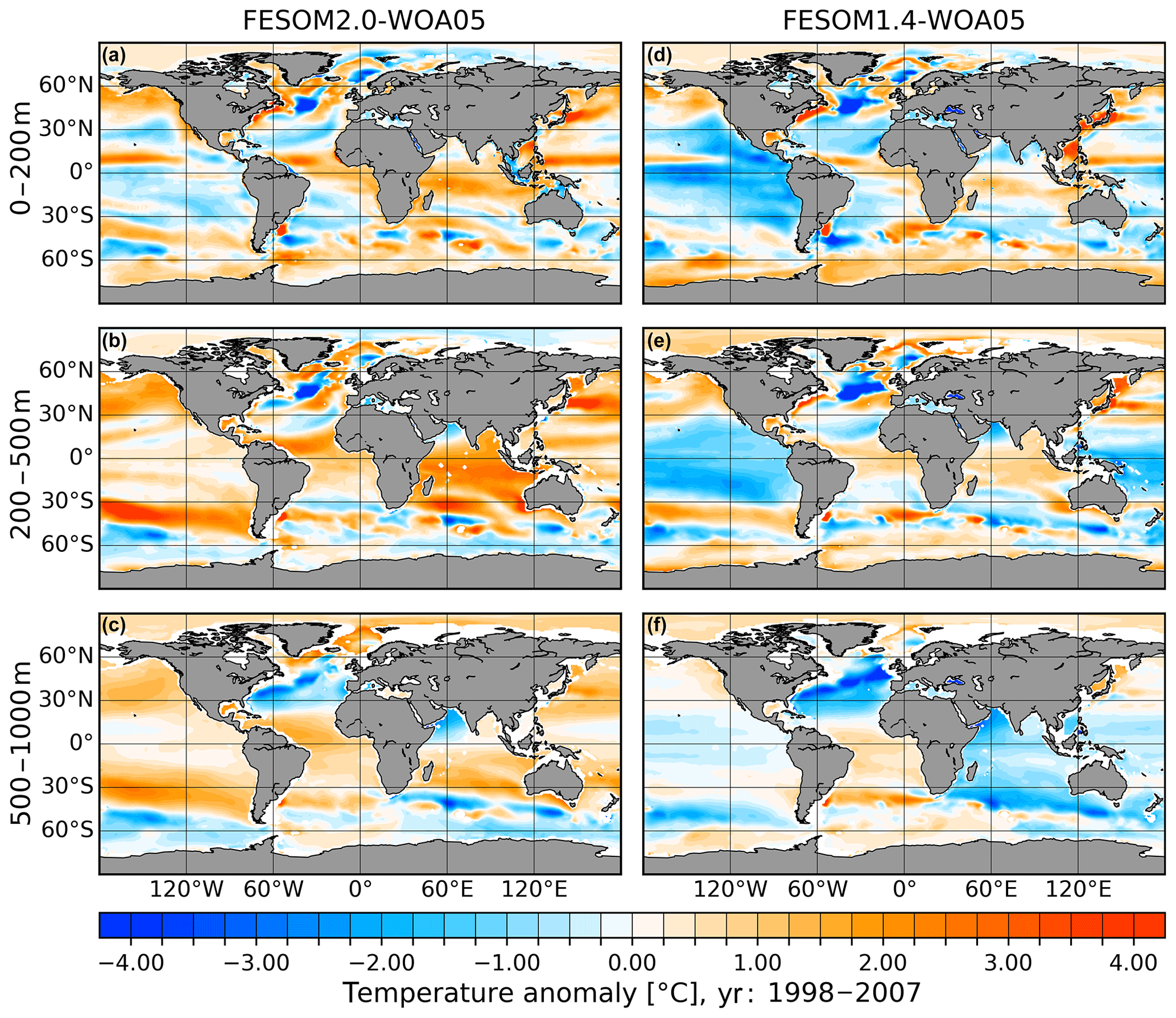
Figure 14 Temperature biases referenced to WOA05 (Locarnini et al., 2006; Antonov et al., 2006) climatology for FESOM2.0 (a–c) and FESOM1.4 (d–f). Model results are averaged over the period of 1998–2007. From top to bottom, averages over three depth ranges are shown: 0–200 m (a, d), 200–500 m (b, e) and 500–1000 m (c, f).

4 Comparison between FESOM1.4 and FESOM2.0

4.1 Differences in hydrography and thermohaline circulation

The purpose of this section is to show that FESOM2.0 has evolved to a point where it is able to reproduce a realistic ocean state that is comparable to its predecessor FESOM1.4. For this purpose, we run both model versions in the linfs configuration using the coarse reference mesh and CORE-II atmospheric forcing. This configuration is used here because it was employed for the systematic assessment of FESOM1.4 in the CORE-II model intercomparison project. Although we use the same 2-D mesh and vertical discretization in both models, it should be kept in mind that FESOM2.0 uses prismatic elements, while FESOM1.4 uses tetrahedral elements, and the numerical cores and the implementation of eddy parameterizations are different.

Figure 15 Same as Fig. 14 but for salinity.

Figure 14 shows the biases of the modeled ocean temperature with FESOM2.0 and FESOM1.4 in three different depth ranges averaged for the period of 1998–2007 and referenced to the WOA05 climatology. FESOM2.0 shows for the surface depth range a stronger warm bias in the area of the East and West Greenland currents and Labrador Current, together with a reduced North Atlantic cold bias. The cold bias in the eastern Pacific is particularly stronger in FESOM1.4. In addition, the surface depth range in FESOM2.0 features a slightly warmer equatorial ocean, North Pacific and Indian Ocean than FESOM1.4, while the situation in the Southern Ocean is reversed. The intermediate depth range simulated with FESOM2.0 shows in general higher warm biases in the northern and southern Pacific, Indian Ocean and in the region of the Kuroshio Current, while the intermediate depth range simulated with FESOM1.4 is dominated by a cool bias for the tropical and subtropical Pacific and North Atlantic. The depth range of 500–1000 m contains for FESOM2.0 a general warming bias except for the Southern Ocean and the North Atlantic. The deep depth range of FESOM1.4 is dominated by a particularly stronger cold bias for the North Atlantic and Indian Ocean, while the biases in the Pacific and Arctic Ocean seem to be smaller.

The salinity biases in the simulations are shown in Fig. 15. Both models indicate a freshening bias for the Arctic Ocean through all considered depth ranges, with the bias in FESOM2.0 being slightly stronger. Both models show quite similar bias patterns for the rest of the global ocean, where the saline biases are more pronounced in FESOM2.0, while the fresh biases are stronger in FESOM1.4.

Figure 16 March (a, b) and September (c, d) MLD (definition after Monterey and Levitus, 1997) averaged over the period of 1998–2007 of FESOM2.0 (a, c, GM, Redi and KPP) and FESOM1.4 (b, d, GM, Redi and KPP) reference simulations.

The northern hemispheric March and southern hemispheric September mean MLD (Monterey and Levitus, 1997) shown in Fig. 16 simulated with FESOM2.0 and FESOM1.4 reveal that FESOM2.0 tends to produce higher and spatially more extended March MLD values in the Labrador Sea and Irminger Sea but also in the GIN seas. In the Southern Hemisphere, the difference is even more pronounced; here, only FESOM2.0 produces significant MLD values in the Weddell Sea, while FESOM1.4 shows almost no MLD activity.

The streamfunctions of the meridional overturning circulation simulated with FESOM2.0 and FESOM1.4 are shown in Fig. 17, globally (upper row), for the Atlantic (middle row) and for the Indo-Pacific region (lower row). It is shown that globally FESOM2.0 tends to produce less AABW with a strength of up to ∼ 5 Sv, compared to FESOM1.4 with a strength of up to 10 Sv, which is at the upper boundary of acceptable values shown by other ocean models (Griffies et al., 2009; Danabasoglu et al., 2016). The FESOM2.0 simulation indicates a stronger northward extent of the AABW cell until ∼ 60^∘ N. The upper AMOC cell, which represents the formation of NADW, is clearly stronger in the FESOM2.0 model simulation, with a strength of 15 Sv compared to 10 Sv in FESOM1.4.

The salinity sections at −30^∘ W from −80^∘ S to 40^∘ N averaged for the period of 1998–2007 (Fig. 18) show that both models are good at reproducing the low-salinity tongue of AAIW that spreads northward. In FESOM2.0, the AAIW reaches slightly less far north than in FESOM1.4, which also does not reach the northward extend of AAIW that the WOA05 data suggest. FESOM2.0 reveals a weaker surface stratification south of −60^∘ S than FESOM1.4. The salinity values below 1000 m depth and south of −50^∘ S in the FESOM2.0 simulation are lower than in FESOM1.4, implying stronger influence from the fresh Antarctic Shelf Water.

In summary, one can say that FESOM2.0 and FESOM1.4 simulate the ocean with a comparable magnitude in the hydrographic biases, although FESOM2.0 tends to have warmer biases, while FESOM1.4 fields are dominated by colder biases. Nevertheless, it should be kept in mind that FESOM1.4 was optimized, improved and tuned over a period of 10 years, while with FESOM2.0 this process is just at the beginning.

4.2 Scaling and performance

Both model versions, FESOM2.0 and FEOSM1.4, are written in Fortran 90 with some C/C$++$ snippets for the binding of third-party libraries. The code of both model versions uses a distributed memory parallelization based on the Message Passing Interface (MPI). One of the main differences between FESOM2.0 and FESOM1.4, besides their finite-volume and finite-element numerical cores, is the treatment of 3-D variables. FESOM1.4 works with 3-D tetrahedral elements. Their vertices are not defined by surface vertices, which require full 3-D lookup tables to address the fields on tetrahedra and 3-D auxiliary arrays for computations of derivatives. FESOM2.0, on the other hand, performs computations in 3-D on prismatic elements, which preserve their horizontal connectivity over depth (see Fig. S4). In this case, 2-D lookup tables are used, which boosts the performance of the model. All simulations shown here were carried out on a Cray CS400 system with 308 compute nodes, where each compute node is equipped with 2x Intel Xeon Broadwell 18-core CPUs with 64 GB RAM (DDR4 2400 MHz), provided by the Alfred Wegener Institute – Helmholtz Centre for Polar and Marine Research. The performance of both model versions on this machine running for one simulated year were tested for a different number of cores and shown in Fig. 19.

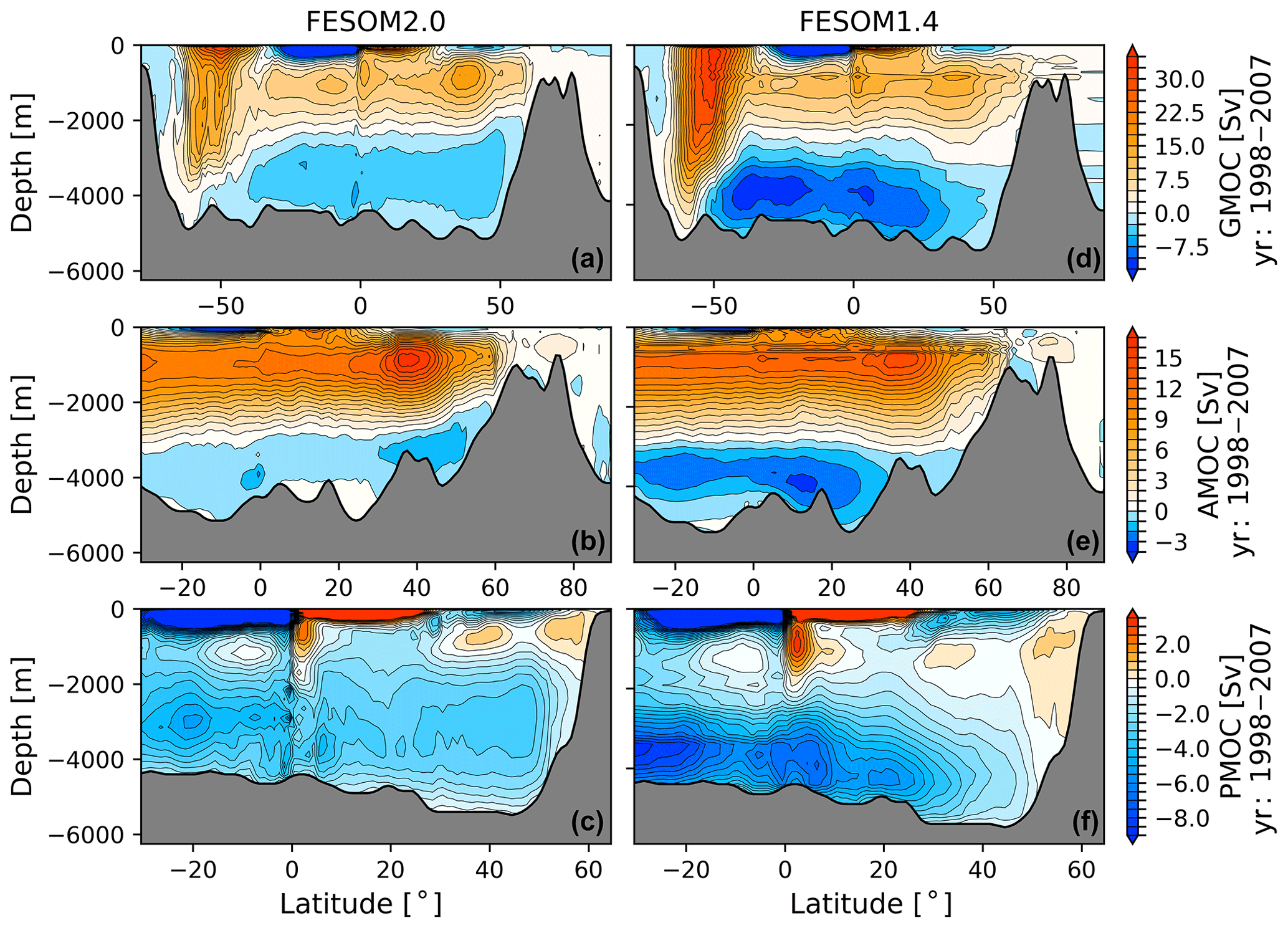
Figure 17 GMOC (a, d), AMOC (b, e) and PMOC (c, f) averaged for the time period of 1998–2007: FESOM2.0 (a–c) and FESOM1.4 (d–f).

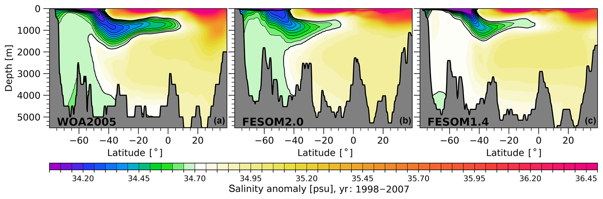
Figure 18 Mean salinity in the vertical section from −80^∘ S, −30^∘ W, to 40^∘ N, −30^∘ W: WOA05 (Locarnini et al., 2006; Antonov et al., 2006) annual climatology (a), FESOM2.0 (b) and FESOM1.4 (c). Model results are averaged for the period of 1998–2007. Contour lines highlight the spreading of Antarctic Intermediate Water (< 34.70 psu) northward.

For the scalability tests, a medium-sized mesh configuration was chosen (see Fig. 1b), which was already used in previous publications, with 638 387 surface vertices and a minimal resolution of 4.5 km in the Arctic (Wang et al., 2018). The performance results were obtained by using the nonlinear free-surface mode, GM and Redi parameterizations and the KPP vertical mixing and taking into account only the time the models require to solve the ocean and sea ice components, disregarding input/output and the initialization phase (setting up arrays, reading the mesh, etc.). Both model versions show a parallel total scalability until at least 2304 cores; beyond that, FESOM2.0 starts to saturate, while FESOM1.4 still reveals linear scalability at least until 4608 cores. The reduction in scalability of FESOM2.0 is partly caused by the sea ice component due to an extensive communication in the elastic–viscous–plastic sea ice solver of FESIM (Danilov et al., 2015). The other source of lacking scalability is the solver for the external mode in the ocean component. We use the parallel Algebraic Recursive Multilevel Solver (pARMS; Li et al., 2003) to iteratively solve for the elevation, which loses scalability towards a large number of cores (not shown). This issue will be addressed in a separate publication. Since the 3-D part of FESOM2.0 is much faster than that of FESOM1.4, the scalability of FESOM2.0 shows earlier saturation, which is limited by 2-D parts in both codes. A general rule of thumb, that holds across a variety of meshes and high-performance computers (HPCs), is that FESOM2.0 scales linearly until around 400 to 300 vertices per core; below that, the scalability starts to slowly deviate from the linear behavior (Koldunov et al., 2019).

Using the low-resolution reference mesh (127 000 surface vertices; Fig. 1a), on 432 cores of the aforementioned machine, neglecting the time for input and output, using a time step of 45 min, FESOM1.4 reaches a throughput of 62 simulated years per day (SYPD), spending 91.9 % and 8.1 % in the ocean step and ice step, respectively. Running the model on the same mesh, with the same computer resources and time step with FESOM2.0, a throughput of 191 SYPD is reached, with the model spending 74.7 % and 25.3 % of its runtime in the ocean step and ice step, respectively. In the ocean step, 16.4 % and 23.4 % of the time is used for the dynamical calculation of u, v, w and SSH, respectively; 39.4 % of the ocean step runtime is used to solve the equations for the temperature and salinity. The implementation of GM following Ferrari et al. (2010) and Redi diffusion accounts for 3.9 % of the ocean step runtime. With the medium-sized mesh configuration (638 387 surface vertices; Fig. 1b) used for the scalability tests, running on 2304 cores with a time steps of 15 min, FESOM1.4 and FESOM2.0 reach a throughput of 20 SYPD and 59 SYPD, respectively.

The numbers given in this section should only serve as a guideline for the performance of FESOM2.0; the details can vary depending on the machine that is used, the frequency of writing the output, the type of advection schemes, the type of mixing schemes and the number of subcycles used in the elastic–viscous–plastic sea ice solver. Nevertheless, a realistic performance estimate for FESOM2.0 is a speedup by a factor of 2.8 to 3.4 compared to FESOM1.4, depending on the aforementioned factors.

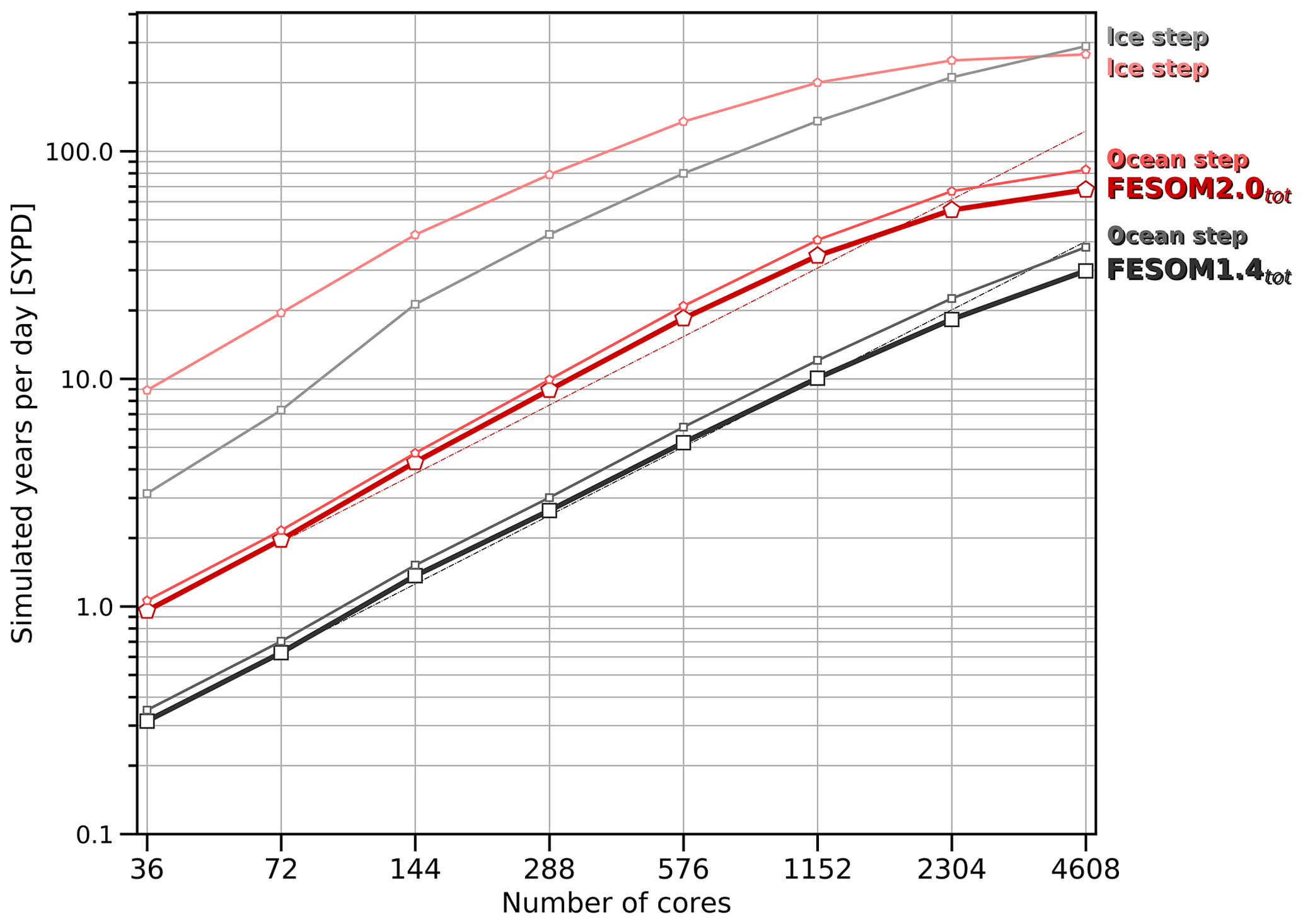
Figure 19 Scaling performance of FESOM1.4 and FESOM2.0 on different number of cores for the medium-sized mesh configuration (see Fig. 1b) with ∼ 0.64 M surface vertices.

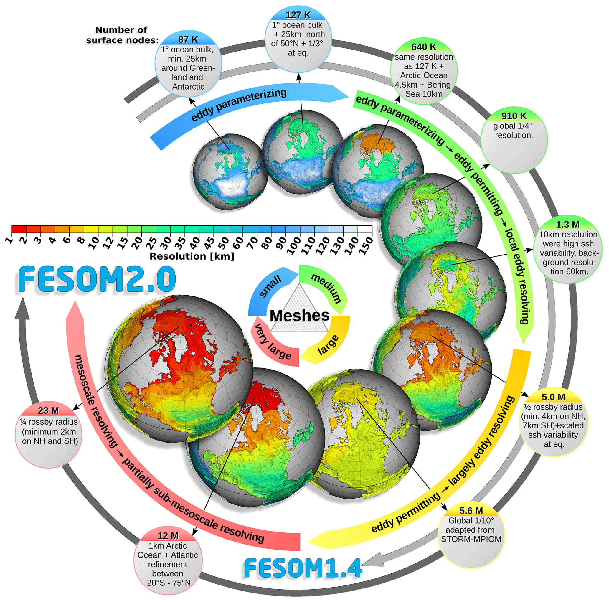
Figure 20 Schematic representation of mesh applicability of FESOM1.4 and FESOM2.0.

4.3 Meshes used

In recent years, as FESOM1.4 had matured from its early days, a large amount of FESOM-based studies had been carried out, covering a wide range of applications and scientific questions, using a large number of very different mesh configurations. Figure 20 gives a schematic of only a small collection of surface unstructured meshes from studies already published or in progress.

The range of available meshes shown in Fig. 20 starts at rather small mesh sizes with less than 250 K surface vertices. For comparison, we mention that a conventional 0.25^∘ (0.5^∘) quadrilateral mesh contains about 1 M (250 K) of wet vertices. These small meshes are used especially for testing and tuning purposes but also for long fully coupled present-day and scenario climate studies (Sidorenko et al., 2014, 2018; Rackow et al., 2016; Wang et al., 2014, 2019a; Sein et al., 2018) and paleo-applications (Shi et al., 2016) with AWI-CM. Using the coarse reference mesh configuration (∼ 127 K surface vertices, also shown in Fig. 1a), it has been shown that FESOM1.4 performs as well as a variety of coarse structured-mesh ocean models, in terms of modeled general ocean circulation (e.g., Danabasoglu et al., 2016; Wang et al., 2016b, c). The range of medium-sized meshes between 500 and 2000 K surface vertices includes the meshes with either globally increased resolution to a higher extent or locally strongly refined key regions of interest (Wang et al., 2016a, 2018a, b, 2019b; Wekerle et al., 2017; Sein et al., 2016, 2018). Using FESOM1.4, it was shown that this class of meshes is well suited for ocean-only simulations, as well as for fully coupled model simulations, which, however, require sufficiently large amounts of computational resources. Using FESOM1.4, Wekerle et al. (2017) and Wang et al. (2018a) have shown that by homogeneously increasing the resolution in the Arctic Ocean to 4.5 km (the mesh with ∼ 640 K surface vertices in Figs. 20 and 1b), the representation of Atlantic water in the Nordic Sea and the Arctic Basin can be significantly improved by only moderately increasing the computational costs. In Sein et al. (2016), FESOM1.4 was used to show that a mesh configuration with increased resolution in dynamically active regions (the mesh with ∼ 1.31 M surface vertices in Fig. 20, minimum resolution 10 km), determined by observed high sea surface height variability, can significantly improve simulated ocean variability and hydrography with respect to observations.

In order to appropriately simulate mesoscale eddies, the Rossby deformation radius needs to be resolved with several grid points (Hallberg, 2013). Sein et al. (2017) introduced a mesh where the Rossby radius is resolved by two grid cells with the minimum resolution set to 4 km in the Northern Hemisphere and 7 km in the Southern Hemisphere (the mesh with ∼ 5.01 M surface vertices; Fig. 20). Another mesh of similar size with a global homogeneous resolution of 1∕10^∘ adapted from the Max Planck Institute ocean model (MPIOM) STORM configuration (von Storch et al., 2012) (∼ 5.58 M surface vertices in Fig. 20) by splitting quads into triangles was also tested. While FESOM1.4 can still be used in these cases, it requires > 7000 cores to reach a throughput of 1.5 SYPD. It became obvious that at around 5 to 6 M surface nodes, FESOM1.4 reaches its practical limit in terms of routinely available computational resources. However, the increased computational performance of FESOM2.0 with 3 times the throughput of FESOM1.4 allows us to use larger meshes to address new research questions. Figure 20 shows two very large upcoming meshes (> 6 M surface vertices) created for FESOM2.0 that were already used in test simulations. One of them focuses on the Arctic Ocean. Since the Rossby deformation radius is latitude dependent, it becomes very small in polar regions, which makes mesoscale-resolving simulations for those regions a challenging task. This configuration consists of ∼ 11.83 M surface vertices, featuring a background resolution of ∼ 1^∘, a latitudinally increasing resolution for the entire Atlantic varying from 0.5 to 1∕15^∘ between −20^∘ S and 75^∘ N, and a mesoscale and partially submesoscale eddy-resolving resolution of 1 km for the entire Arctic Ocean. The other mesh configuration consists of ∼ 23.18 M surface vertices and resolves the Rossby deformation radius with four grid cells on a global scale with a cutoff resolution of 2 km for the Northern Hemisphere and Southern Hemisphere.

The upcoming version of AWI-CM using FESOM2.0 will allow us to also expand the mesh applicability for long climate simulations from small-sized towards medium- and large-sized mesh configurations.

5 Discussion and conclusions

Currently, FESOM2.0 possesses all the features available in FESOM1.4 and offers more flexibility, which results mainly from the ALE implementation of the vertical coordinate in the new model version. Although many features are common between the two versions, applying the same surface forcing and initial conditions leads to certain differences in modeled ocean states. These differences result in part from the slightly different implementation of parameterization schemes and consequently the different set of tuning parameters. This includes the implementation of GM after Ferrari et al. (2010) (i.e., solving a boundary-value problem on eddy-induced transport streamfunction) in FESOM2.0 and after Griffies et al. (1998) (i.e., using the skew flux formulation for eddy-induced transport) in FESOM1.4. Part of the differences can also originate from the implicit numerical mixing associated with different numerics in the two versions of the model. The analysis of the numerical mixing in FESOM2.0 associated with advection schemes will be described in another paper.

The comparison between FESOM1.4 and FESOM2.0 in terms of hydrography proved that FESOM2.0 is at a stage where it is ready to replace FESOM1.4. Both model versions show a similar magnitude of the biases in temperature and salinity. There are spatial differences, however, especially in the Pacific and Indian oceans, which can be attributed to general differences in the numerical cores as well as different implementation of schemes like the GM parameterization. The meridional overturning between FESOM1.4 and FESOM2.0 reveals some obvious differences, especially in the case of the AMOC. Here, FESOM2.0 simulates a significantly stronger upper AMOC cell, with a strength of ∼ 15 Sv, while FESOM1.4 is known to simulate a weaker upper AMOC cell (Sidorenko et al., 2011), with a strength of ∼ 10 Sv, which is at the lower range of acceptable values simulated by other ocean models (Griffith et al., 2009). Observational AMOC estimates suggest an AMOC strength of ∼ 17.5 Sv at 26^∘ N (Smeed et al., 2014; McCarthy et al., 2015), which is much closer to the simulated value of FESOM2.0.

It is worth mentioning that the analysis of transport is significantly simplified in FESOM2.0 as compared to that in FESOM1.4. In the continuous finite-element discretization of FESOM1.4, the interpretation of fluxes is ambiguous since the model equations are discretized in a weak sense through weighting with some test functions. This makes it difficult to perform the analysis of overturning circulation or even the volume fluxes from the computed velocities without the usage of additional techniques for the proper flux interpretation (see, e.g., Sidorenko et al., 2009). In FESOM2.0, the model fluxes are explicitly defined and their interpretation is straightforward.

FESOM1.4 had a throughput that is around 3 times lower compared to regular-grid models of similar complexity. With the 3-fold increase in computational performance of FESOM2.0, we are now able to offer for the first time an unstructured-mesh model that is able to run as fast as or even faster than regular-mesh models. For example, Prims et al. (2018) show that the state-of-the-art NEMO model in a 1∕4^∘ configuration is able to obtain around 3 SYPD using 512 cores; however, scalability is already lost when going to a higher number of cores. Using the same number of cores on the aforementioned machine, with a mesh that has a resolution of 1∕4^∘ (the mesh with ∼ 910 K surface vertices in Fig. 20), FESOM2.0 reaches a throughput of more than 5 SYPD.

FESOM2.0 can reach such a high throughput because the unstructured nature of its meshes is confined to the horizontal direction, while the vertical direction is structured and prismatic elements are used. In this case, lookup tables and the corresponding auxiliary arrays are only two-dimensional and need to be accessed just once and can then be used over the entire water column. This makes the cost of accessing them rather low compared to FESOM1.4. We suspect that unstructured-mesh models also benefit from the fact that only wet nodes are accessed, which could partly explain why FESOM2.0 outperforms some models using structured meshes.

Development of FESOM2 will continue during the next few years. The external vertical mixing library CVMIX will be added into FESOM2.0 and tested, including the new energy-consistent vertical mixing parameterization IDEMIX (Olbers and Eden, 2017; Eden and Olbers, 2017; Pollman et al., 2017). The development of the new coupled system AWI-CM using FESOM2.0 is finished in support for a variety of climate-scale applications with time frames from paleo- to future scenarios as required by the climate research community. The final tuning for the new AWI-CM is underway. The development team also works on new higher order advection schemes for tracer and momentum. Although for the moment only the usage of the linear free-surface and full free-surface options is implemented in the code with the ALE approach, the implementation of terrain-following and hybrid coordinates will follow.

Despite the existing remarkable computational performance of FESOM2.0, there is still potential for future improvements by tackling performance bottlenecks, such as by calling the sea ice step just every second or other ocean step, which could help to delay scalability saturation in the sea ice component due to the elastic–viscous–plastic (EVP) subcycling, as well as to explore the use of subcycling for the sea surface height solver. However, these potential performance improvements will be explored in a separate publication. Further improvements may include the use of hybrid meshes composed of triangles and quads (Danilov et al., 2014), which could reduce the number of edge cycles and further speed up the code performance.

This paper is the first in a series of papers to document the development and assessment of important key components of FESOM2.0 in realistic global model configurations. We described the implementation and associated simulation biases of some simple ALE options, that is, the linear free-surface and full free-surface formulations. Furthermore, we discussed the effect of GM parameterization, isoneutral Redi diffusion and KPP versus PP vertical mixing schemes. In particular, the relative roles of the GM and Redi diffusion parameterizations are assessed. The paper also shows that the results of FESOM2.0 compare well to FESOM1.4 in terms of model biases and ocean circulation but with a remarkable performance speedup by a factor of 3 mainly due to its superior data structure. In addition, FESOM2.0 shows a more realistic AMOC strength, combined with a convenient computation of transport.