Assessment of the Finite-VolumE Sea ice–Ocean Model (FESOM2.0) – Part 2: Partial bottom cells, embedded sea ice and vertical mixing library CVMix

The second part of the assessment and evaluation of the unstructured-mesh Finite-volumE Sea ice–Ocean Model version 2.0 (FESOM2.0) is presented. It focuses on the performance of partial cells and embedded sea ice and the effect of mixing parameterisations available through the Community Vertical Mixing (CVMix) package.

It is shown that partial cells and embedded sea ice lead to significant improvements in the representation of the Gulf Stream and North Atlantic Current and the circulation of the Arctic Ocean. In addition to the already existing Pacanowski and Phillander (fesom_PP) and K-profile (fesom_KPP) parameterisations for vertical mixing in FESOM2.0, we document the impact of several mixing parameterisations from the CVMix project library. Among them are the CVMix versions of Pacanowski and Phillander (cvmix_PP) and K-profile (cvmix_KPP) parameterisations; the tidal mixing parameterisation (cvmix_TIDAL); a vertical mixing parameterisation based on turbulent kinetic energy (cvmix_TKE); and a combination of cvmix_TKE and the recent scheme for the computation of the Internal Wave Dissipation, Energy, and Mixing (IDEMIX) parameterisation. IDEMIX parameterises the redistribution of internal wave energy through wave propagation, non-linear interactions and the associated imprint on the vertical background diffusivity. Further, the benefit from using a parameterisation of Southern Hemisphere sea ice melt season mixing in the surface layer (MOMIX) for reducing Southern Ocean hydrographic biases in FESOM2.0 is presented. We document the implementation of different model components and illustrate their behaviour. This paper serves primarily as a reference for FESOM users but is also useful to the broader modelling community.

1 Introduction

Global unstructured-mesh ocean models start to be widely used in climate studies, including the recent CMIP6 simulations (Semmler et al., 2020), although structured-mesh ocean general circulation models are still more mature in terms of features, functionality and complexity due to their long development history. However, the unstructured-mesh ocean models also gradually acquire new features and catch up in their functionality. This paper continues the work by Scholz et al. (2019) in documenting the features available in Finite-volumE Sea ice–Ocean Model version 2.0 (FESOM2.0, Danilov et al., 2017). It focuses on two aspects. The first is about partial bottom cells and embedded sea ice, both of which essentially rely on the arbitrary Lagrangian Eulerian (ALE) vertical coordinates used in FESOM2.0. The second deals with mixing parameterisations enabled through the use of the Community Ocean Vertical Mixing (CVMix, Griffies et al., 2015; Van Roekel et al., 2018) package.

Partial bottom cells were first introduced for a finite-volume model by Adcroft et al. (1997) as an attempt to improve the representation of the bottom topography in general ocean circulation models. Adcroft et al. (1997) introduces partial bottom cells as a compromise solution between the less accurate but computationally efficient full-cell approach and the very accurate but computationally expensive shaved-cell approach. Partial bottom cells are implemented in FESOM2.0 by using the vertical ALE approach of FESOM2.0 numerical core documented in Danilov et al. (2017).

Another feature made available through using ALE in FESOM2.0 is related to the sea ice–ocean interaction. Naturally, sea ice, more precisely the loading of sea ice, contributes to the ocean pressure. However, in many ocean models, especially in the absence of surface mass fluxes or on fixed vertical grids, the loading is omitted and sea ice is treated as “levitating”. The option to consider sea ice loading is now implemented into FESOM2.0, which is called “embedded” sea ice and was first mentioned by Hibler et al. (1998) and later further introduced by Hutchings et al. (2005) and Campin et al. (2008). They state that the advection of sea ice in combination with the coupling of embedded sea ice through ice loading can be an important source of ocean variability especially in the vicinity of ice edges (Campin et al., 2008). The implementation of embedded sea ice relies on the zstar vertical coordinate option in FESOM2 and also on the fact in the moment that the sea ice component is called on each time step of the ocean model, using the standard Elastic Viscous Plastic (EVP) method of Hunke and Dukowicz (1997), applying 150 EVP subcycles (Koldunov et al., 2019).

Diapycnal mixing in the ocean is an essential process that acts on the ocean stratification and the distribution of heat; salt; and passive tracers like nutrients, biological agents, or CO₂. Various processes contributing to diapycnal mixing can act with different magnitudes over a wide range of horizontal and vertical scales, from several kilometres down to centimetres (Robertson and Dong, 2019). Due to the finite discretisation scale in all ocean models, the mixing processes can not be resolved and thus must be parameterised. The parameterisations of diapycnal mixing can be done in a variety of ways with different complexity, such as boundary layer schemes like the K-profile parameterisation of Large et al. (1994) or turbulent closure schemes like the one of Gaspar et al. (1990) and many others. A great innovation in the ocean modelling community is the development of software packages that contain a variety of vertical mixing parameterisations in a format that makes it easy to integrate them into existing model code (Fox Kemper et al., 2019). One of these software packages is the Community Ocean Vertical Mixing package (CVMix, Griffies et al., 2015; Van Roekel et al., 2018), which has now been integrated into FESOM2.0. CVMix is tailored to be used in state-of-the-art climate models to produce vertical profiles of diffusivity and viscosity (Fox Kemper et al., 2019), providing a comparable mixing implementation over a wide spread of different ocean models, such as MOM6, POP, MPAS and ICON. Such effort makes it easier to compare these models to each other. From the CVMix package we implemented the parameterisation scheme of Pacanowski and Philander (1981), the K-profile parameterisation of Large et al. (1994), and the tidal mixing parameterisation of Simmons et al. (2004). Further, the infrastructure of the CVMix library has been used to implement the turbulent kinetic energy (TKE) scheme of Gaspar et al. (1990) and the scheme for Internal Wave Energy, Dissipation and Mixing (IDEMIX) of Olbers and Eden (2013) in the same way as was done in Gutjahr et al. (2020). It should be mentioned that neither TKE nor IDEMIX is yet part of the official CVMix package but will hopefully be added to the package in the future.

Beside the prime vertical mixing schemes, like the K-profile scheme, the Pacanowski and Phillander scheme, and others that have the purpose of creating a general mixing parameterisation for the entire ocean, and vertical mixing schemes, like the tidal mixing scheme of Simmons et al. (2004) or IDEMIX that are used to parameterise internal wave processes that then result in a heterogeneous background diffusivity, there are also mixing parameterisations that aim at resolving regional processes. One of them was proposed by Timmerman and Beckmann (2004). It parameterises the wind-driven mixing in the Southern Ocean, especially when there is insufficient mixing during the melt seasons when other mixing schemes are used. It is used in FESOM2.0 to improve the otherwise too low stratification in the Southern Ocean and Weddell Sea.

The intention of this paper is to document the performance of the newly implemented features, i.e. partial bottom cells, embedded sea ice, the vertical mixing parameterisations that come with the implementation of CVMix, and the local mixing parameterisation of Timmerman and Beckmann (2004), based on comparing the associated hydrographic biases, changes in vertical convection and differences in the meridional overturning circulation using a relatively coarse reference mesh.

The paper is structured as follows. In Sect. 2 we describe the mesh configuration and model setup used in the simulations. The description and analysis of partial bottom cells, embedded sea ice and vertical mixing schemes is done in Sect. 3. A discussion and conclusion is given in Sect. 4.

2 Model configurations

We use the FESOM2.0 coarse-mesh configuration core2, which is the same mesh as in Part 1 of this paper. It consists of ∼ 0.13 M surface vertices, with a nominal resolution of 1^∘ in the bulk of the ocean, ∼ 25 km north of 50^∘ N, $\mathrm{1}/\mathrm{3}$^∘ in the equatorial belt and slightly enhanced resolution in the coastal regions. In the vertical, 48 unevenly distributed layers are used, with a vertical grid spacing increasing stepwise from 5 m at the surface to 250 m towards the bottom.

All model simulations are initialised from the Polar Science Center Hydrographic winter Climatology (PHC3.0, updated from Steele et al., 2001) and forced by the CORE interannually varying atmospheric forcing fields (Large and Yeager, 2009) for the period 1948–2009. For each simulation a spin-up over three full CORE cycles was applied, where each subsequent cycle was initialised with the final results from the preceding cycle. All modelled data shown in this work are averaged over the period 1989–2009.

All model simulations, except the one with the turbulent kinetic energy (TKE) closure mixing of Gaspar et al. (1990), use a non-constant latitude-dependent vertical background diffusivity with values between 10⁻⁴ and 10⁻⁶ m² s⁻¹, as described in Scholz et al. (2019). Further, all simulations use the Monin–Obukhov length dependent vertical mixing parameterisation of Timmermann and Beckmann (2004) in the surface boundary layer south of −50^∘ S. The effect of this parameterisation on the simulated ocean state in FESOM2.0 is described in Sect. 3.4. The horizontal viscosity is computed via a modified harmonic Leith approach (Fox-Kemper and Menemenlis, 2008) plus a biharmonic background viscosity (0.01 m² s⁻¹) . For coarse-mesh setups, like the one used here, FESOM2.0 uses the Gent–McWilliams (GM) parameterisation for eddy stirring (Gent et al., 1995; Gent and Mcwilliams, 1990), and we follow the implementation of Ferrari et al. (2010). The isoneutral tracer diffusion (Redi, 1982) coefficient equals to that of GM, as is the case in Scholz et al. (2019) and in previous FESOM versions (Wang et al., 2014). GM and Redi are scaled with horizontal resolution with a maximum value of 3000 m² s⁻¹ at 100 km horizontal resolution and change linearly to zero between a resolution of 40 and 30 km. In the vertical, they are scaled according to Ferrari et al. (2010) and Wang et al. (2014). The simulations use as default the K-profile parameterisation for vertical mixing (KPP, Large et al., 1994), a linear free surface (Scholz et al., 2019), levitating sea ice and a full bottom cell approach, unless otherwise stated.

3 FESOM2.0 model components and evaluation

3.1 Partial bottom cells

The concept of partial cells as an attempt to improve the bottom representation in general ocean circulation models was first introduced for the finite-volume approach by Adcroft et al. (1997). Although an early version of partial cells was developed by Cox (1977) and used by Semtner and Mintz (1977) and Maier-Reimer et al. (1993), it has never been officially released (Griffies et al., 2000). Adcroft et al. (1997) presented three different cases. The first case is the conventional full-cell approach, where the depth of the ocean bottom is approximated with the nearest standard depth level of the vertical model discretisation. The second case is the partial-cell approach in which the bottom level can take any intermediate depth within the cell, thus capturing water columns more accurately. In these two cases, the bottom features a “stepped” topography, and the jump between the steps is smaller for the partial-cell approach (Adcroft et al., 1997). The third case introduced by Adcroft et al. (1997) is a shaved-cell approach, which assumes a constant slope within each bottom cell and gives the best approximation for a continuous bottom topography. Adcroft et al. (1997) showed that the shaved-cell approach gives the most accurate results, but induces a significant increase in computational demand, whereas the partial-cell approach is a good compromise between the low computational demand of the full-cell approach and the increased accuracy of the shaved-cell approach. Hence, most ocean models (e.g. NEMO, MOM6, MPAS, POP) including FESOM2.0 went in favour of the partial-cell approach.

For the implementation of partial cells in FESOM2.0, we follow the work of Pacanowski and Gnanadesikan (1998), who implemented partial cells for the B-grid discretisation in MOM2 with efforts to minimise pressure gradient errors and spurious diapycnal mixing. They addressed that calculating horizontal pressure gradients needs some special attention for partial cells since not all grid points within the bottom layer are at the same depth. In FESOM2.0, we compute pressure gradient force based on the density Jacobian approach as used by Shchepetkin (2003) and not the pressure Jacobian approach proposed by Pacanowski and Gnanadesikan (1998). The density Jacobian approach is less prone to pressure gradient error than using pressure Jacobian, and therefore the model is more stable. Furthermore, we limited the thickness of the partial bottom cell to be at least half of the full-cell layer thickness to reduce the possibility of violating the vertical Courant–Friedrichs–Lewy (CFL) criterion, especially in shallow regions.

Using a B-grid-like discretisation, where the scalars are located at vertices of a triangular mesh while the velocities are located at the centroids of the triangular elements, makes it necessary to define the partial cells at both locations. First, the partial bottom depth is defined at the centroids of the triangular elements based on the real bottom topography considering the aforementioned limitation. Following this, the vertex partial bottom depth is derived from the deepest partial bottom of the surrounding triangular elements (see the schematic representation in Fig. S1 in the Supplement).

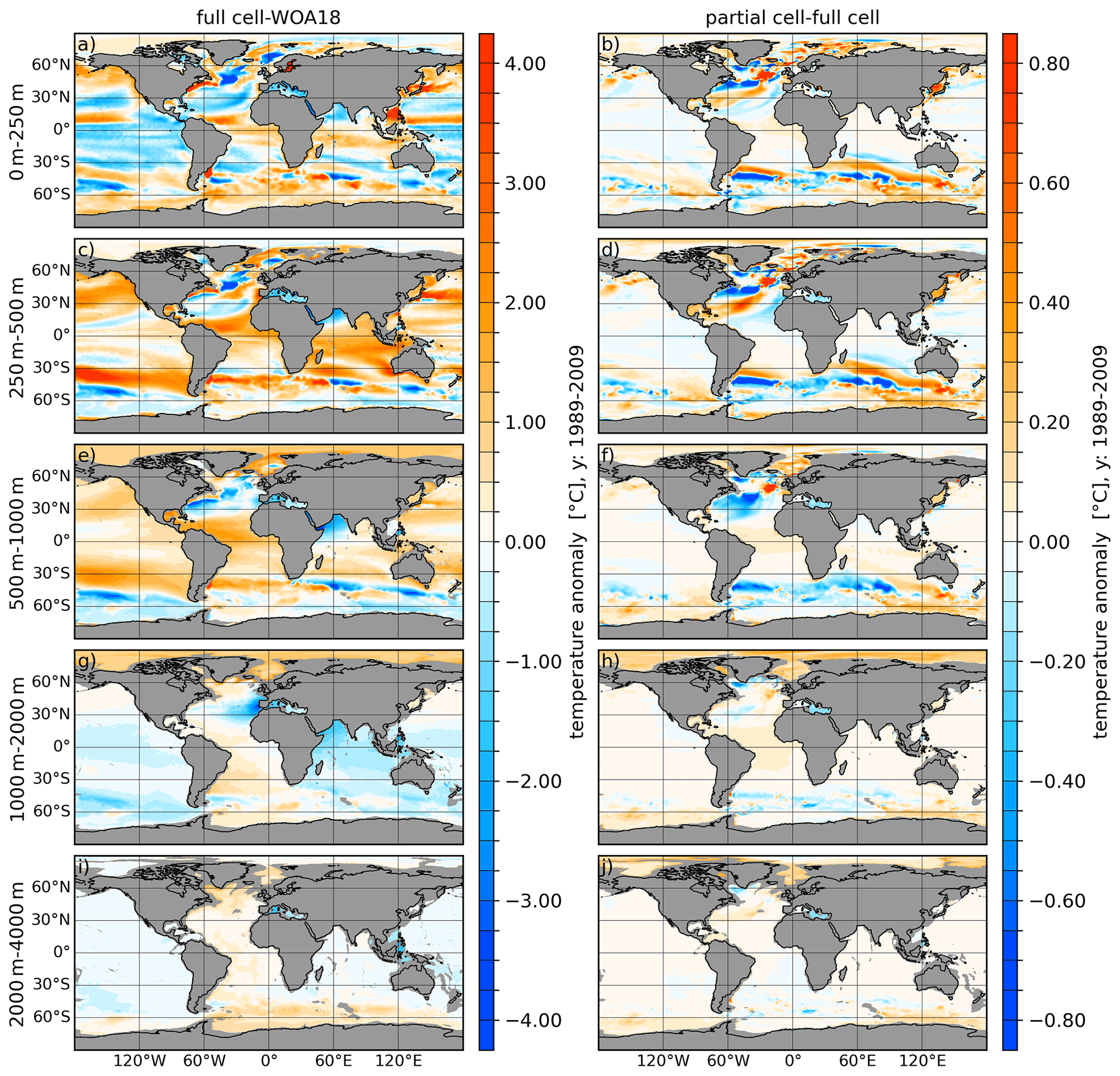
Figure 1 (a, c, e, g, i) Temperature biases of full cells referenced to the World Ocean Atlas 2018 (WOA18, Zweng et al., 2019) averaged over the period 1989–2009. (b, d, f, h, j) The temperature difference between partial and full cells (partial minus full). From top to bottom the panels show the vertically averaged fields for the depth ranges of 0–250, 250–500, 500–1000, 1000–2000 and 2000–4000 m.

In order to demonstrate the effect of the partial cells on the simulated ocean state we performed two model simulations using the full-cell and partial-cell approaches, respectively. We first investigate the temperature biases of the full-cell approach with respect to the data of the World Ocean Atlas 2018 (WOA18; Locarnini et al., 2019; Zweng et al., 2019; Fig. 1a, c, e, g and i), and second we investigate the temperature differences between partial cell and full cell (partial minus full) averaged over five different depth ranges 0–250, 250–500, 500–1000, 1000–2000 and 2000–4000 m (Fig. 1b, d, f, h and j).

The full-cell setup (Fig. 1a, c, e, g and i) shows positive climatological temperature bias in the northern and southern Pacific, the Atlantic equatorial ocean and the central Indian Ocean through the depth ranges of 0–250, 250–500 and 500–1000 m. In the same depth ranges there are also negative biases in the North Atlantic (NA) subtropical gyre and in the equatorial and southern subtropical Pacific. The depth ranges of 250–500 and 500–1000 m indicate cold biases in the Southern Ocean (SO) and around the coast of Antarctica. The deeper depth ranges (1000–2000 and 2000–4000 m.) indicate small negative temperature biases in most of the world oceans, except for the Atlantic Ocean and Arctic Ocean (AO), which both possess a small warming bias in the depth ranges. The Arctic warming anomaly at these depths originates largely from a vertically overextended Atlantic water inflow branch (not shown), which is a typical feature of coarse-resolution models (e.g. Ilicak et al., 2016).

Using partial cells (Fig. 1b, d, f, h and j) leads to profound changes, especially at the position of zonal fronts in the North Atlantic and South Atlantic. In the depth ranges of 0–250, 250–500 and 500–1000 m in the NA, partial cells lead to a cooling in the Labrador Sea (LS) and Irminger Sea (IS), as well as along the path of the Gulf Stream (GS) and North Atlantic Current (NAC), except for the area around 50^∘ N, −30^∘ W, which is characterised by warming. In the upper South Atlantic (SA), partial cells lead to a northward shift of Brazil–Malvinas Confluence Zone expressed by a dipole of warmer South Atlantic Current (SAC) and cooler Antarctic Circumpolar Current (ACC). Further, partial cells lead to a predominant cooling in the SO Atlantic sector and parts of the Indian Ocean sector, while the Pacific sector of the SO and most of the Antarctic coastal areas are dominated mostly by warming anomalies. The Arctic Ocean features a slight warming anomaly at all depths except for the surface when using partial cells instead of full cells. The Table S1 in the Supplement shows the regional (35^∘ N < lat < 70^∘ N,−80^∘ W < long < 5^∘ E,) temperature standard deviation and root-mean-square error with respect to WOA18, with and without partial cells. It proves that partial cells lead to a significant improvement, especially in the upper and intermediate ocean depth range, while the biases in the very deep ocean marginally increase.

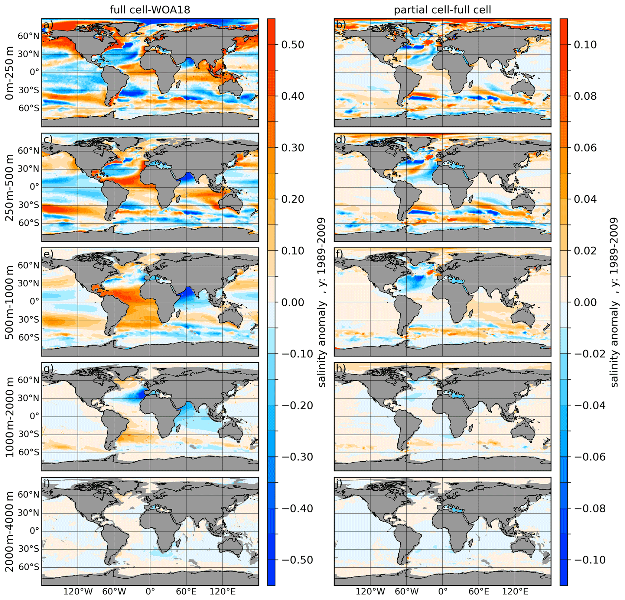
Figure 2 The same as Fig. 1 but for salinity.

Figure 2 shows the same information as Fig. 1 but for salinity. Here the full cell run indicates a generally fresher AO for the surface and the 250–500 m depth range with respect to WOA18. Further negative salinity biases can be found within the upper three depth ranges in the equatorial Pacific, northern and southern subtropical Atlantic, at the position of the Atlantic northwestern corner, in the northern Indian Ocean (IO), and parts of the SO. Strong positive salinity biases with full cells can be found in the surface depth range of the North Pacific and in the Chukchi and Beaufort seas. Further positive salinity biases in the 250–500 and 500–1000 m depth ranges are found along the pathway of the Gulf Stream, as well as in the equatorial Atlantic and central IO. The deep depth range of 1000–2000 m has positive salinity anomalies in the northern and southern Atlantic and negative salinity biases in the Mediterranean outflow branch and IO.

Using partial cells leads to an increase in salinity throughout all depth ranges of the AO relative to using full cells. Further, a salinity increase at the position of the “cold blob” in the Greenland–Iceland–Norwegian (GIN) seas, in the eastern South Atlantic and parts of the SO can be observed within the upper three depth ranges. Compared to full cells, using partial cells reduces salinity along the pathway of the GS, the Antarctic Circumpolar Current (ACC) in the South Atlantic and along the coast of Antarctica.

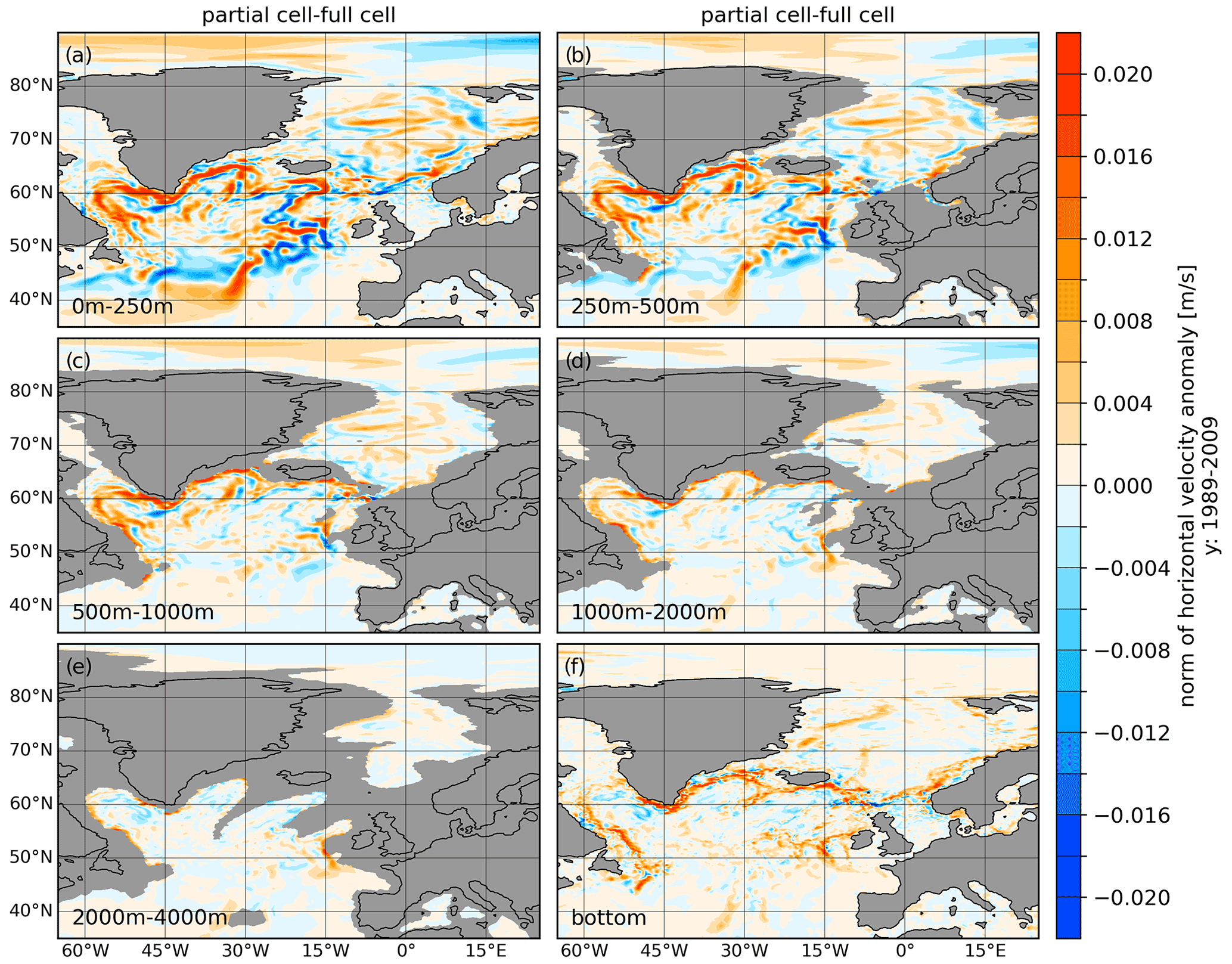
Figure 3 Difference of the horizontal velocity norm between simulations with partial and full cells (partial minus full) averaged over the period 1989–2009 and averaged over the depth ranges of 0–250, 250–500, 500–1000, 1000–2000, and 2000–4000 m and the bottom value.

The differences in the horizontal velocity speed between partial and full cells (Fig. 3) for the depth ranges of 0–250, 250–500, 500–1000, 1000–2000, 2000–4000 m and at the bottom reveal that the velocity in the East Greenland Current (EGC), West Greenland Current (WGC) and Labrador Current (LC) are stronger by up to 0.02 m s⁻¹ through all depth ranges presented here with partial cells. The upper differences reveal that partial cells lead to a weakening and a slight southwards shift of the NAC between −45 and −30^∘ W and a more pronounced tendency towards a northwest bend of the NAC between −30 and −15^∘ W, which is nevertheless still too far eastward. By using partial cells the pathway of the Irminger Current (IC) moves closer to the continental slope.

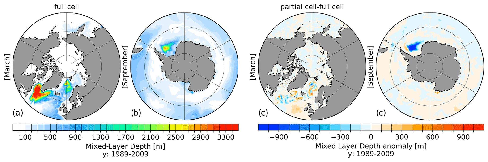
Figure 4 Northern Hemisphere March (a) and Southern Hemisphere September (b) mixed-layer depth (MLD) with full cells and corresponding anomalous MLD with partial minus full cells (c, d) averaged for the period 1989–2009.

In terms of absolute Northern Hemisphere and Southern Hemisphere maximum MLD using full cells (Fig. 4a and b), FESOM2.0 features known intensive convection in the Labrador Sea and Irminger Sea, northern Greenland Sea, and the central Weddell Sea (Marshall and Schott, 1999; Sallée et al., 2013; Danabasoglu et al., 2014).

The anomalous Northern Hemisphere and Southern Hemisphere maximum MLD using partial cells features a slight MLD decrease in the southern LS, IS and northern Greenland–Iceland–Norwegian (GIN) seas and a slight MLD increase along the pathway of the IC and in the southern and central GIN seas (Fig. 4c). In the Southern Hemisphere, partial cells have a more pronounced effect, leading to a significant (up to 1000 m) decrease in MLD in the central Weddell Sea (WS) and a minor increase in MLD of around 300 m along the eastern continental slope of the Antarctic Peninsula.

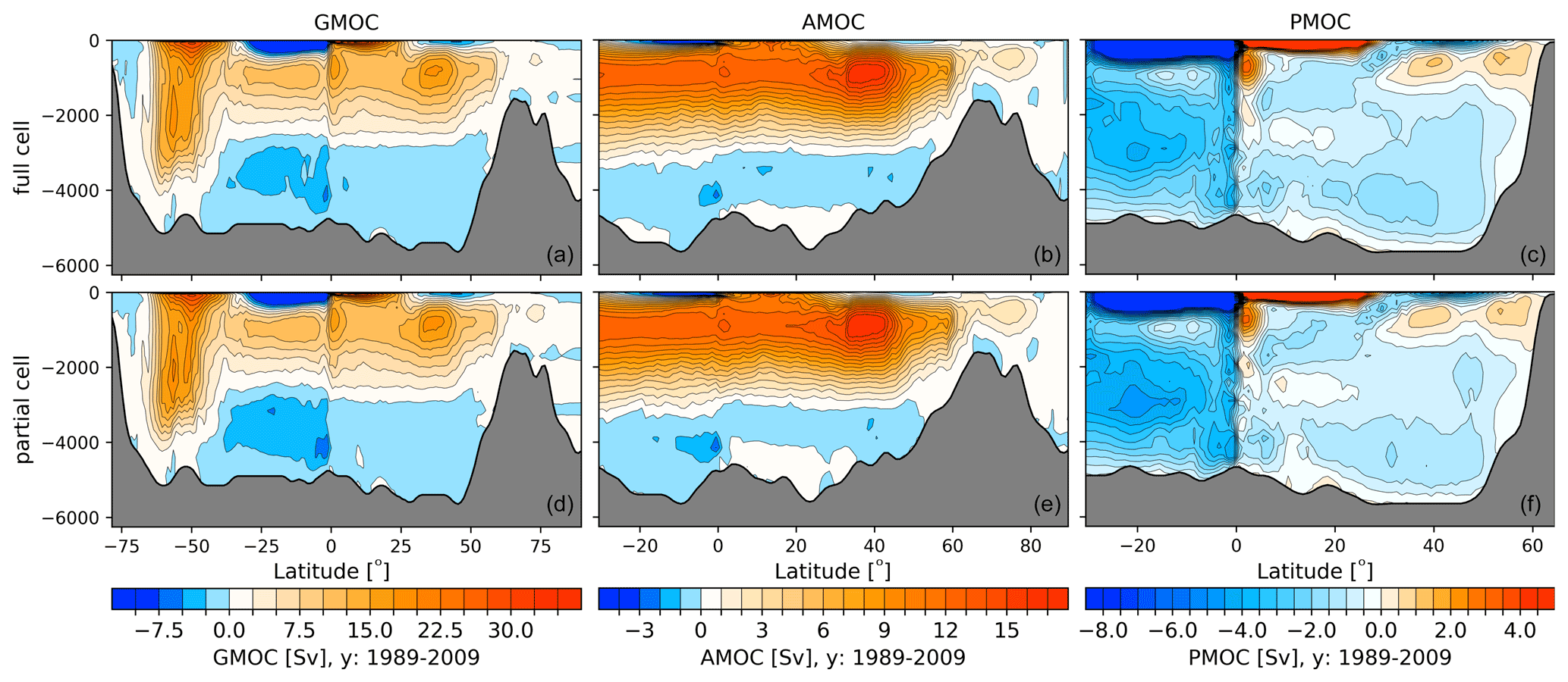
Figure 5 Global (GMOC, a, d), Atlantic (AMOC, b, e) and Indo-Pacific (PMOC, c, f) meridional overturning circulations for full cells (a–c) and partial cells (d–f) averaged for the time period 1989–2009.

The differences between using full cells and partial cells with the global, Atlantic and Indo-Pacific meridional overturning circulations (Fig. 5) are rather small, with magnitudes of less than 1 Sv. Both cases feature an upper AMOC circulation cell of ∼ 16 Sv and an Antarctic Bottom Water (AABW) cell with strength between −1 and −2 Sv. One can summarise this by stating that partial cells lead to an improvement of the circulation pattern, especially regarding the reduced zonality of the Gulf Stream and NAC branch, even in rather coarsely resolved configurations.

3.2 Embedded sea ice

As described in Scholz et al. (2019), FESOM2.0 supports the full free surface formulation with two possible options, zlevel and zstar (Adcroft and Campin, 2004). Both options allow for surface freshwater exchanges that can modify the thickness of the surface layer and thus decrease or increase salinity in the surface layer. This avoids the need for virtual salinity fluxes, which are required in the linear free surface (linfs) approach when the layer thicknesses are kept fixed. Using virtual salinity fluxes has the potential to affect the model integrity on long timescales and change local salinities with certain biases (Scholz et al., 2019).

In reality, part of sea ice is embedded in the ocean, which has an impact on the ocean pressure below. In the model, when the sea ice loading is omitted, the levitating sea ice (Campin et al., 2008) does not impose pressure on the ocean. This is the default case in the case of linfs but also applicable to zlevel and zstar. The other case when ice loading is considered has embedded sea ice (Rousset et al., 2015), which depresses the sea surface according to its mass. Since it affects the layer thicknesses, this case is only available for the full free surface cases of zlevel and zstar. Although freezing and melting have no direct effect on the oceanic pressure, the divergence of the ice transport does modify the ice-loading fields and influences the hydrostatic pressure (Campin et al., 2008). As mentioned by Campin et al. (2008), this effect could be compensated by the divergence of the oceanic transport in the special case where sea ice and ocean velocities match, but in reality sea ice and ocean velocities are not identical, especially in the presence of high-frequency wind forcing. Therefore, sea ice dynamics in combination with the ice-loading coupling can be a source of oceanic variability, especially near the ice edge where ice divergence and convergence are large (Campin et al., 2008). However, using embedded sea ice harbours the risk that the amount of sea ice loading due to excessive accumulation and the resulting depression in the surface elevation may result in a depletion of the surface layer thickness, as only the surface layer is allowed to change when the zlevel option is used. To avoid this issue, we limit the maximum ice loading in FESOM2.0 to a sea ice height of 5 m when the zlevel option is used. When using zstar the problem is less severe, since there the change in elevation is distributed over all vertical layers except for the bottom one. This makes zstar the recommended option when using embedded sea ice, as also stated by Campin et al. (2008).

To show the effect of embedded sea ice on the simulated ocean state, two simulations were carried out using the zstar option of FESOM2.0, one with levitating sea ice (omitting the effect of sea ice loading on ocean pressure) and the other with embedded sea ice (including the effect of sea ice loading on ocean pressure).

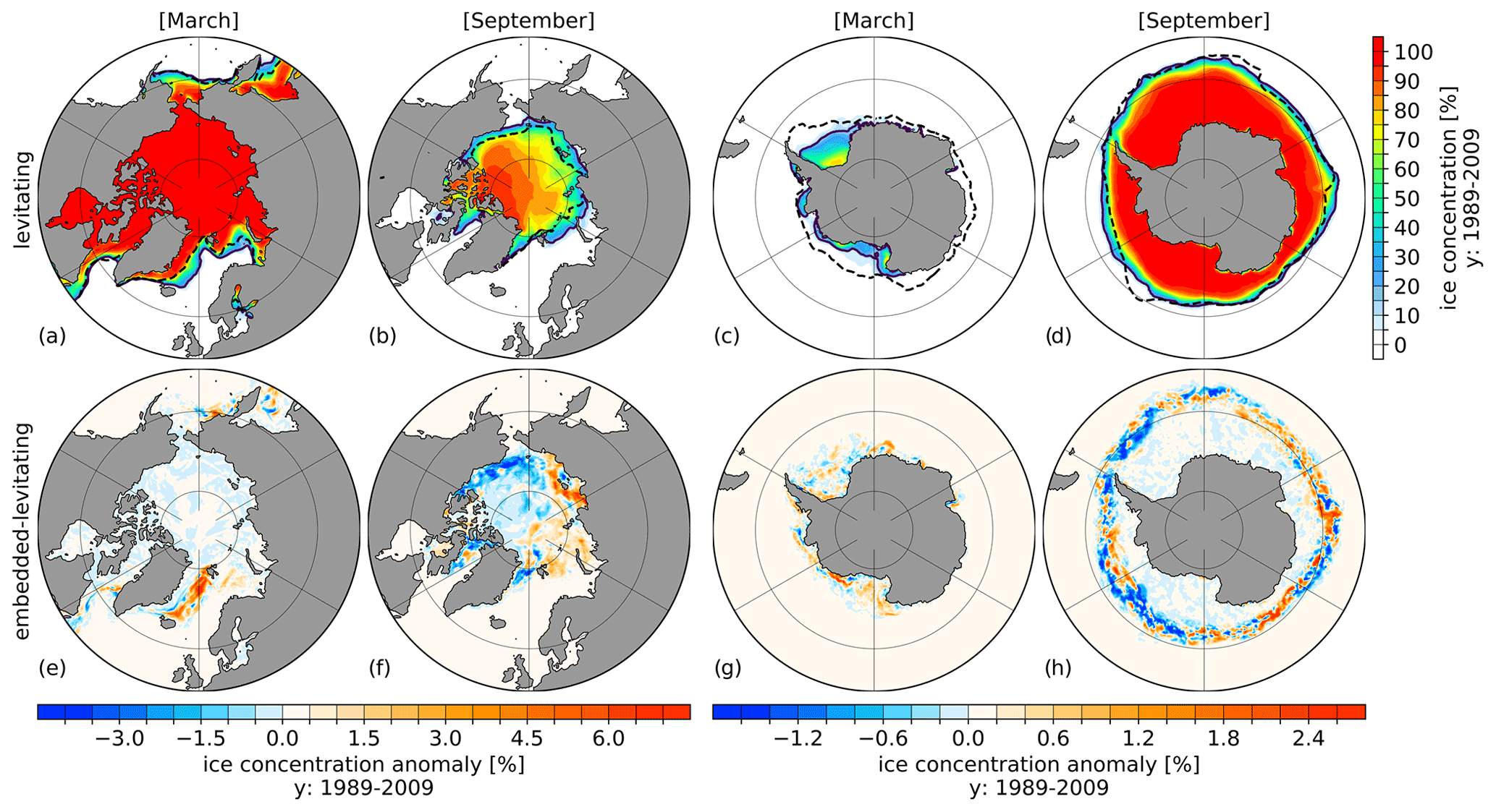
Figure 6 Levitating (a–d) Northern Hemisphere and Southern Hemisphere March (a, c) and September (b, d) sea ice concentration averaged for the period 1989–2009. Solid and dashed lines indicate the simulated and observed (Cavalieri et al., 1996) contour of the 15 % sea ice extent, respectively. The lower row shows the corresponding sea ice concentration anomalies between embedded and levitating sea ice (embedded minus levitating) averaged over the same period.

Figure 6 shows the sea ice concentration (SIC) for March and September in the levitating sea ice case and the difference between the embedded and levitating sea ice cases. Superimposed are the simulated (solid) and observed (dashed, Cavalieri et al., 1996) contour line of the 15 % sea ice extent. The Northern Hemisphere March sea ice edge (Fig. 6a) shows a good agreement with observational data for the LS, IS and Bering Sea but reveals a extension in the Greenland Sea and Barents Sea that is too far southwards. The simulated Northern Hemisphere (September) sea ice extent (Fig. 6b) is larger than the observations. The Southern Hemisphere (March) sea ice extent is underestimated in the simulation, while the simulated Southern Hemisphere (September) sea ice extent is in good agreement with the observation.

Using the embedded sea ice leads to an increase in the SIC in the Greenland Sea by around 6 % in March. In September, embedded sea ice leads to positive SIC anomalies in the eastern AO and negative anomalies in the western AO. In the Southern Hemisphere, embedded sea ice leads to a heterogeneous pattern of small positive and negative changes along the sea ice edge. The corresponding results for the sea ice thickness are shown in Fig. S3​​​​​​​ in the Supplement; here both March and September Northern Hemisphere sea ice thickness anomalies reveal a dipole-like pattern with reduced sea ice thickness in the area of the Beaufort gyre and increased sea ice thickness in the eastern AO and the region of the transpolar drift when using embedded sea ice.

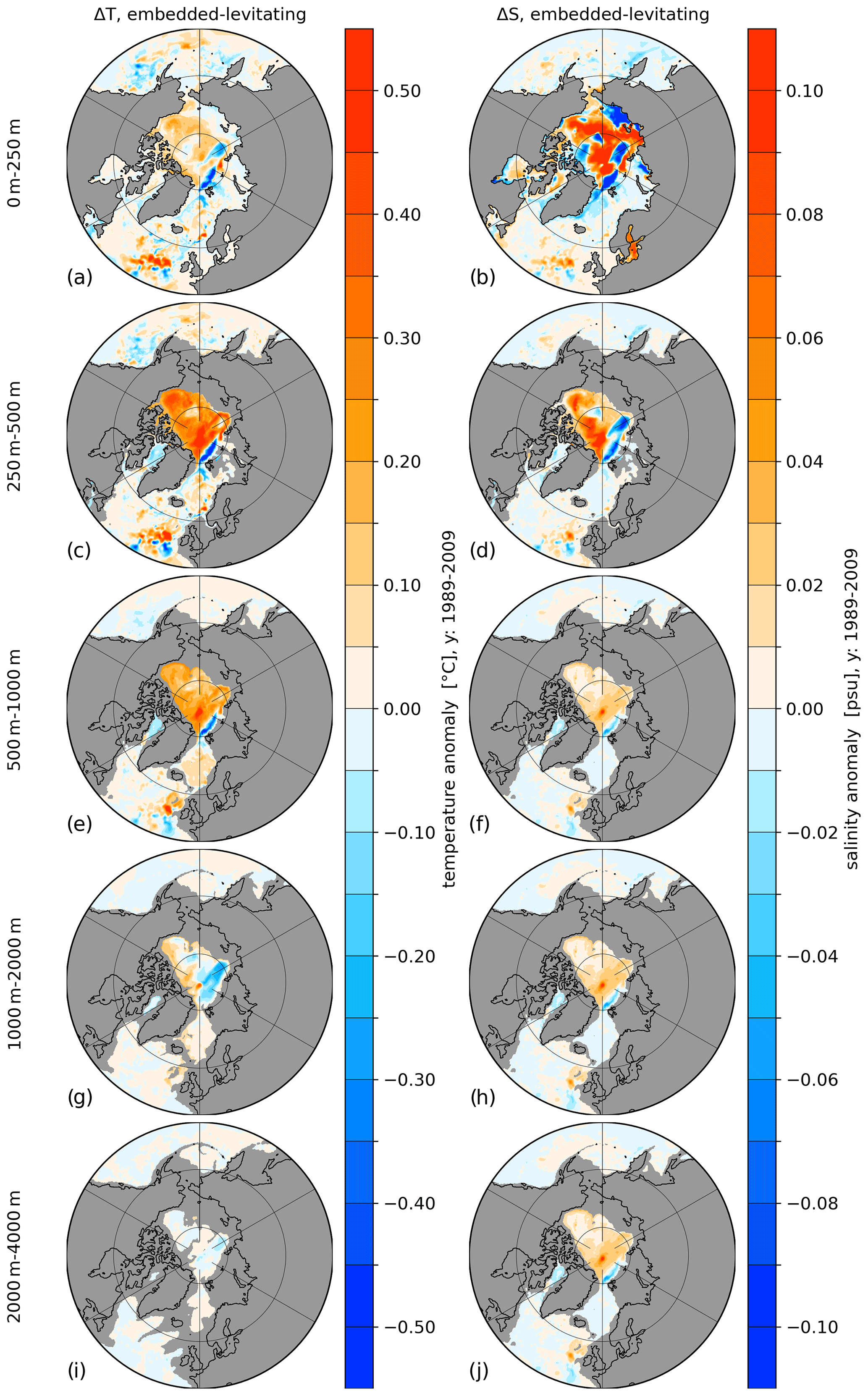
Figure 7 Temperature (a, c, e, g, i) and salinity (b, d, f, h, j) difference between embedded and levitating sea ice averaged for the period 1989 to 2009. Panels show, from top to bottom, the vertically averaged fields for the depth ranges of 0–250, 250–500, 500–1000, 1000–2000 and 2000–4000 m.

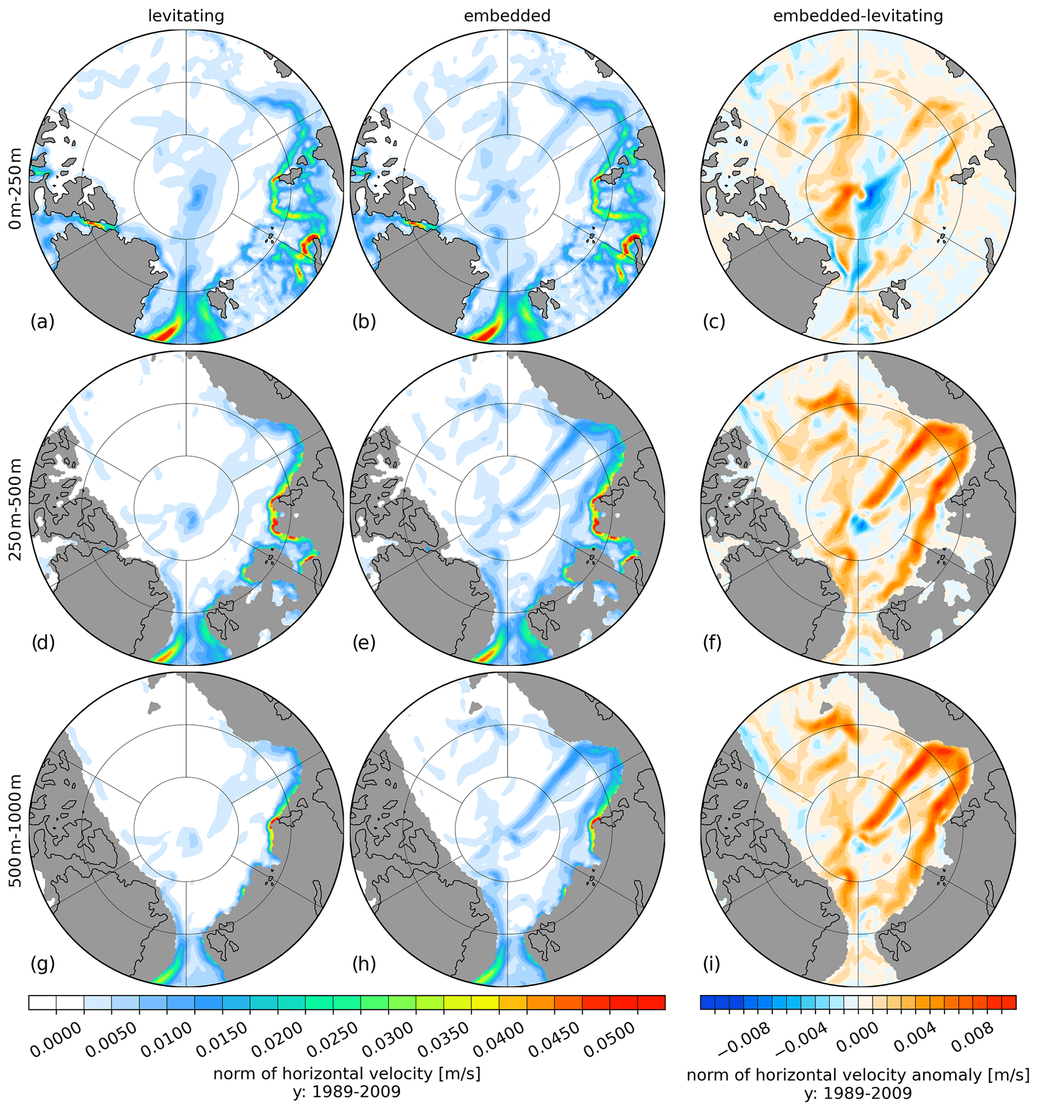
Figure 8 Norm of ocean velocity for levitating sea ice (a, d, g) and embedded sea ice (b, e, h) and the difference between embedded and levitating sea ice (c, f, i) averaged for the period 1989 to 2009. The panels show, from top to bottom, the vertically averaged fields for the depth ranges of 0–250, 250–500 and 500–1000 m.

Regarding the changes in the ocean, Fig. 7 shows the temperature (Fig. 7a, c, e, g and i) and salinity (Fig, 7b, d, f, h and j) differences between the embedded and levitating (embedded minus levitating) sea ice cases averaged over the depth ranges 0–250, 250–500, 500–1000, 1000–2000 and 2000–4000 m. The temperature and salinity differences reveal that significant warming of up to 0.5 ^∘C and a salinification of up to 0.10 psu occur in almost the entire AO due to embedded sea ice, except in a thin stripe along the eastern continental shelf of the AO that shows negative anomalies in the depth ranges of 0–250, 250–500 and 500–1000 m. The changes in temperature and salinity can be explained by the changes in ocean currents. Figure 8 depicts the speed of the horizontal currents in levitating (Fig. 8a, d and g) and embedded (Fig. 8b, e and h) sea ice cases, as well as their difference (Fig. 8c, f and i). Using embedded sea ice leads to an increase in the speed along the entire boundary current of the Eurasian Basin and along the Lomonosov Ridge that can be found in all three presented depth ranges. The increase in the velocity of the boundary currents caused by using embedded sea ice leads to an enhanced heat and salt transport in the Atlantic water layer originating from the Fram Strait, which results in a warmer and more saline intermediate depth in the Arctic Ocean (Fig. S4 in the Supplement). The increase in temperature and salinity, especially in the surface layers of the AO using embedded sea ice, reduces existing local biases (see Figs. 1 and 2) that occur when using levitating sea ice. On the whole, it can be stated that using embedded sea ice instead of levitating sea ice has a significant effect on the ocean dynamics of the AO but no effect in the Southern Ocean or Antarctic marginal seas.

3.3 Implementation and evaluation of vertical mixing schemes

In addition to the already existing Pacanowski and Philander (fesom_PP, Pacanowski and Philander, 1981) and MOM4 K-profile (fesom_KPP, Large et al., 1994) vertical mixing parameterisations in FESOM2.0 that were based on the implementation in the predecessor version FESOM1.4, the vertical mixing parameterisations of the Community Vertical Mixing (CVMix, Griffies et al., 2015) project have been now added as well. This includes the CVMix vertical mixing of Pacanowski and Philander (cvmix_PP); the POP (Parallel Ocean Program) K-profile (cvmix_KPP) parameterisation; the tidal mixing parameterisation of Simmons et al. (2004) (cvmix_TIDAL); and the turbulent kinetic energy (cvmix_TKE) mixing of Gaspar et al. (1990) in combination with the Internal Wave Dissipation, Energy, and Mixing (IDEMIX) parameterisation (Olbers and Eden, 2013; Eden and Olbers, 2014). Although cvmix_TKE and IDEMIX are not yet a part of the CVMix project, they use its libraries in the background and will join the project in the future. CVMix is used by a variety of models, such as MOM6, POP, MPAS and ICON, and provides an opportunity of a cross-model vertical mixing implementation that allows for an enhanced cross-model intercomparison.

3.3.1 Comparison of cvmix_KPP and cvmix_PP with previous fesom_KPP and fesom_PP implementations

In FESOM2.0 we implemented cvmix_PP and cvmix_KPP in addition to the previous implementations fesom_PP and fesom_KPP that were adopted from FESOM1.4. The difference between cvmix_PP and fesom_PP lies in the background coefficient for viscosity, which is considered in cvmix_PP but not in fesom_PP when computing the diffusivity, following the experience with FESOM1.4, which did not need to be more diffusive. The difference between cvmix_KPP and fesom_KPP lies mainly in the treatment of the squared velocity shear and buoyancy difference with respect to the surface, although CVMix does not make any specific requirements here. In cvmix_KPP we synchronised the implementation with our project partner models MPIOM and ICON-o and compute the cvmix_KPP surface quantities by averaging over 10 % of the boundary layer depth as recommended by Griffies et al. (2015), while in fesom_KPP the surface values are linked to the first layer in the model, which was inspired by the implementation in the older MOM4.

Figure S5 in the Supplement displays the temperature (first and second column) and salinity (third and fourth column) biases of fesom_KPP with respect to WOA18 (first and third column) as well as the difference between fesom_PP and fesom_KPP (second and fourth column). In the surface depth range the climatological temperature and salinity biases of fesom_KPP with respect to WOA18 are largely negative in the tropical Pacific, subtropical Pacific, North Atlantic, South Atlantic, and AO and positive in the tropical Atlantic Ocean, tropical Indian Ocean, Southern Ocean, Labrador Sea, GIN seas and the marginal seas of the North Pacific. The subsurface depth ranges of 250–500 and 500–1000 m are dominated by largely positive temperature biases, except for the Southern Ocean, the pathway of the GS and NAC, and the northern Indian Ocean. The salinity biases in the 250–500 and 500–1000 m depth range largely preserve the pattern from the surface layer except for an increasing and expanding positive salinity bias in the tropical Atlantic, reduced positive salinity biases in the Indian Ocean and northern Pacific and reduced negative biases in the Arctic Ocean. The 1000–2000 m depth range features small warm biases in the AO and GIN seas, positive temperature and salinity biases in the LS and the South Atlantic, negative temperature and salinity biases in the eastern North Atlantic (possibly due to weak Mediterranean outflow), and small negative temperature and salinity biases in the Pacific and Indian Ocean. The very deep depth range of 2000–4000 m reveals rather small warming bias for the entire Atlantic and SO.

The results of fesom_KPP and fesom_PP produced rather small temperature and salinity differences (note the different colour bar ranges between the first and second and third and fourth column) when considering the biases with respect to the WOA18 climatology. Employing fesom_PP has the tendency to be slightly warmer almost everywhere in the subsurface layers, slightly saltier in the AO, and fresher in the surface layer of the subtropical and equatorial ocean compared to using fesom_KPP. Looking at the maximum MLD between fesom_PP and fesom_KPP (Fig. S6 in the Supplement) it can be seen that fesom_PP has the tendency to produce an up to 500 m shallower deep convection in LS and WS when compared to fesom_KPP.

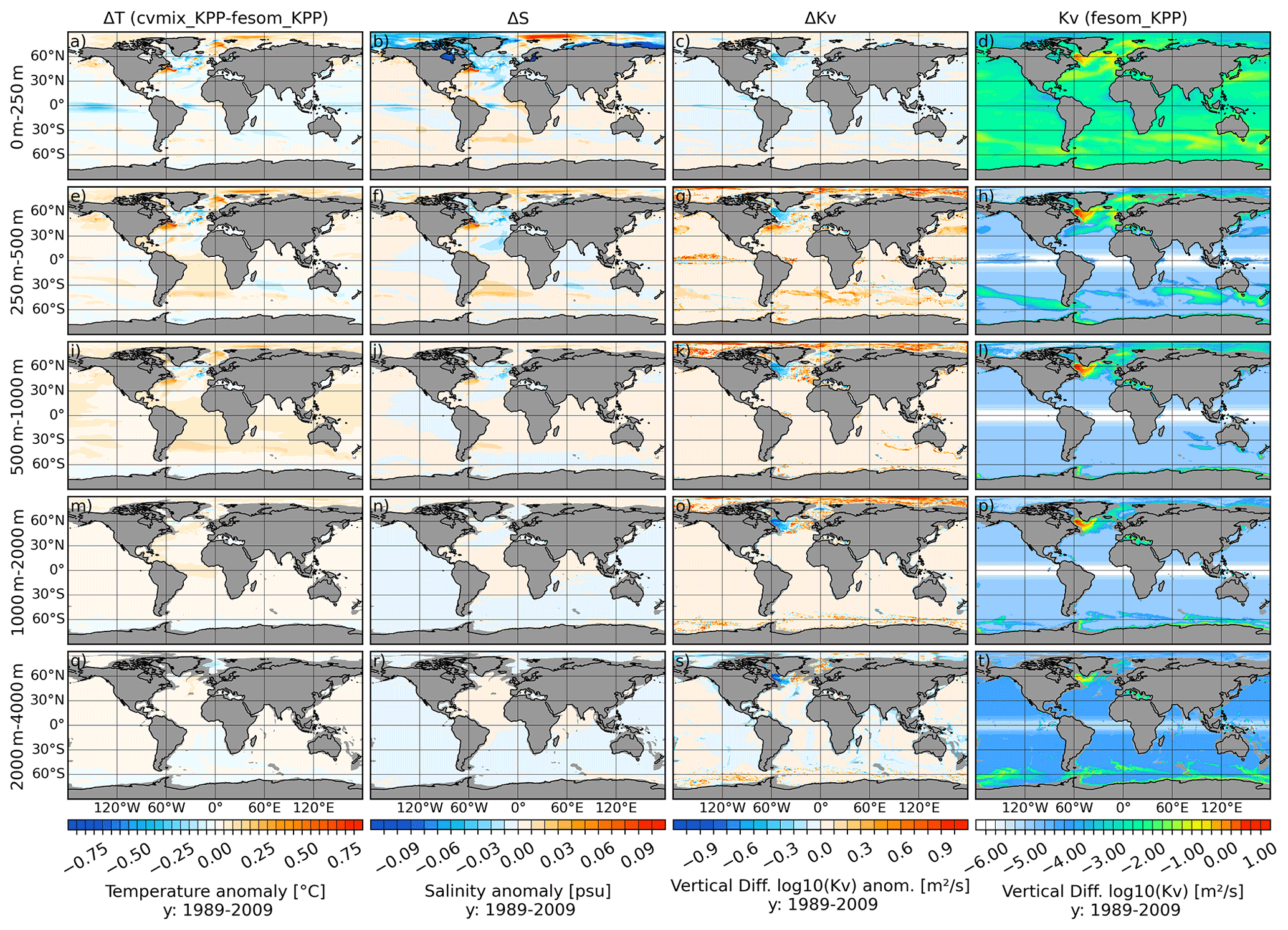
Figure 9 Temperature (a, e, i, m, q), salinity (b, f, j, n, r) and vertical diffusivity (c, g, k, o, s) difference between cvmix_KPP and the original fesom_KPP implementation, as well as the absolute vertical diffusivity values (d, h, l, p, t) for fesom_KPP averaged for the period 1989 to 2009. The panels show, from top to bottom, the vertically averaged fields for the depth ranges of 0–250, 250–500, 500–1000, 1000–2000 and 2000–4000 m.

Figure 9 shows the difference in temperature (Fig. 9a, e, i, m and q), salinity (Fig. 9b, f, j, n and r) and vertical diffusivity (Fig. 9c, g, k, o and s) between cvmix_KPP and fesom_KPP (cvmix_KPP minus fesom_KPP) averaged over five different depth ranges. Figure 9d, h, l, p and t present the fesom_KPP vertical diffusivity as a reference. The temperature and salinity differences are also rather small here compared to the climatological biases shown in Fig. S5 in the Supplement. The cvmix_KPP results have the tendency to show a slightly fresher surface ocean in the marginal seas of the AO, while the central AO shows an increase in salinity by ∼ 0.1 psu.

The absolute value of the vertical diffusivity in fesom_KPP is larger than that in cvmix_KPP in the surface layers and in regions of unstable stratification (buoyancy frequency < 0) superimposed on a non-constant background diffusivity as described in Scholz et al. (2019). The different treatment of the squared velocity shear and buoyancy difference with respect to the surface in cvmix_KPP leads to a reduction in the vertical diffusivity (Fig. 9c, g, k, o and s) in the Labrador and Irminger seas and to an increase in the AO locally by up to an order of magnitude (especially in the deep ocean).

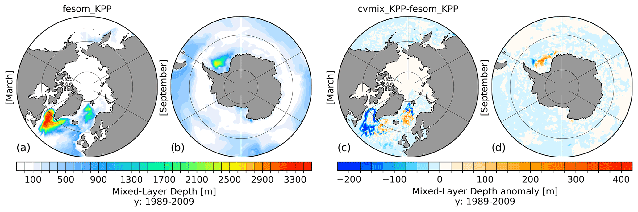
Figure 10 Northern Hemisphere March (a) and Southern Hemisphere September (b) mixed-layer depth (MLD) for the fesom_KPP implementation and the corresponding anomalous MLD between cvmix_KPP and fesom_KPP implementation (c, d) averaged for the period 1989–2009.

The differences in MLD between fesom_KPP and cvmix_KPP are presented in Fig. 10, where Fig. 10a and b shows the absolute MLD value for fesom_KPP in the Northern Hemisphere in March and in the Southern Hemisphere in September, respectively. Figure 10c and d display the corresponding anomalies between cvmix_KPP and fesom_KPP (cvmix_KPP-fesom_KPP). The absolute MLD values for fesom_KPP in March show high values of up to 3300 m in the entire LS and parts of the Irminger Sea, intermediate values of up to 2000 m in the northern and eastern GIN seas, and values of ∼ 900 m along the eastern continental slope of the North Atlantic. In the Southern Hemisphere in September, fesom_KPP simulates a large MLD of ∼ 2500 m in the central Weddell Sea and weaker MLD of ∼ 500 m in the band of the Antarctic Circumpolar Current (ACC). Compared to the fesom_KPP, cvmix_KPP leads to a ∼ 200 m weaker MLD in the boundary currents of the LS, southern LS and along the northeastern continental slope of the GIN seas and slightly larger MLD values in the IS and southwestern GIN seas. The KPP ocean boundary layer depth (OBLd, Large et al., 1994) for fesom_KPP and the difference in OBLd between cvmix_KPP and fesom_KPP is additionally presented in Fig. S7 in the Supplement, where it is shown that cvmix_KPP produces an around 150 m shallower OBLd, which is largely attributed to the different treatment of the surface quantities by averaging over 10 % of the boundary layer depth.

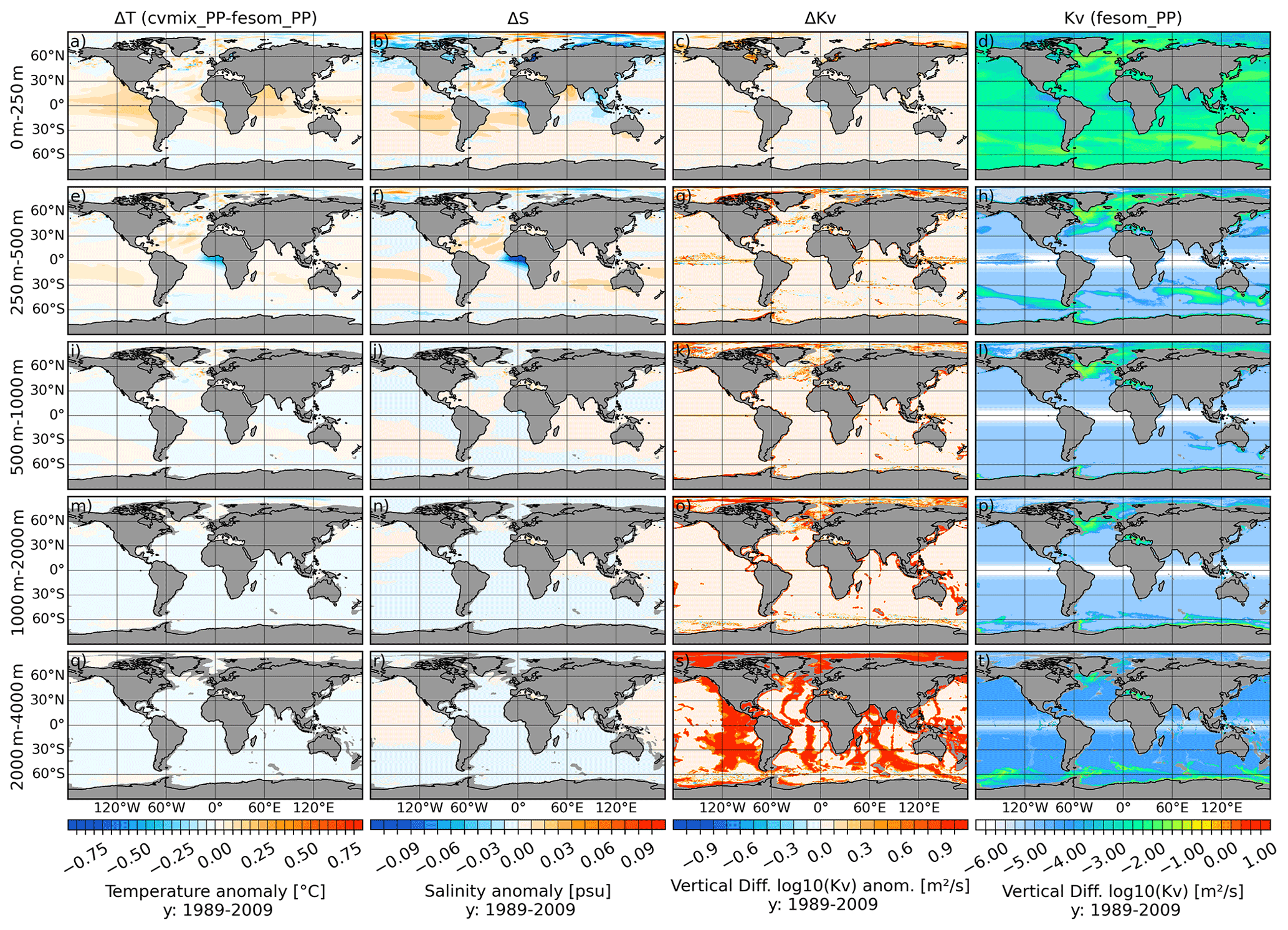
Figure 11 Temperature (a, e, i, m, q), salinity (b, f, j, n, r) and vertical diffusivity (c, g, k, o, s) difference between cvmix_PP and original fesom_PP implementation, as well as the absolute vertical diffusivity values (d, h, l, p, t) for fesom_PP averaged for the period 1989 to 2009. The panels show, from top to bottom, the vertically averaged fields for the depth ranges of 0–250, 250–500, 500–1000, 1000–2000 and 2000–4000 m.

Figure 11 presents the differences in temperature (Fig. 11a, e, i, m and q), salinity (Fig. 11b, f, i, n and r) and vertical diffusivity Kv (Fig. 11c, g, k, o and s) between cvmix_PP and fesom_PP (cvmix_PP minus fesom_PP), as well as the absolute values of vertical diffusivity for fesom_PP (Fig. 11d, h, l, p and t). For the upper two surface depth ranges, cvmix_PP shows an overall small warming anomaly, except for the Gulf of Guinea in the 250–500 m depth range where the anomaly is negative. The salinity with cvmix_PP has overall only slight positive anomalies, except for coastal Arctic areas and the Gulf of Guinea, which both indicate a slight freshening anomaly when compared to fesom_PP. The depth ranges below 500 m show no significant temperature or salinity differences between cvmix_PP and fesom_PP. The absolute value of Kv in fesom_PP also shows larger values all over the surface layer and in the areas of unstable stratification similar to fesom_KPP but with a lower magnitude and a more extended region of increased Kv in the LS and IS. The Kv difference between cvmix_PP and fesom_PP shows sporadically positive values along the coastal Arctic Ocean and in parts of the North Atlantic and GIN seas. As one would expect, cvmix_PP has an order of magnitude larger values in the very deep ocean layer where the background viscosity enters the computation of Kv in cvmix_PP.

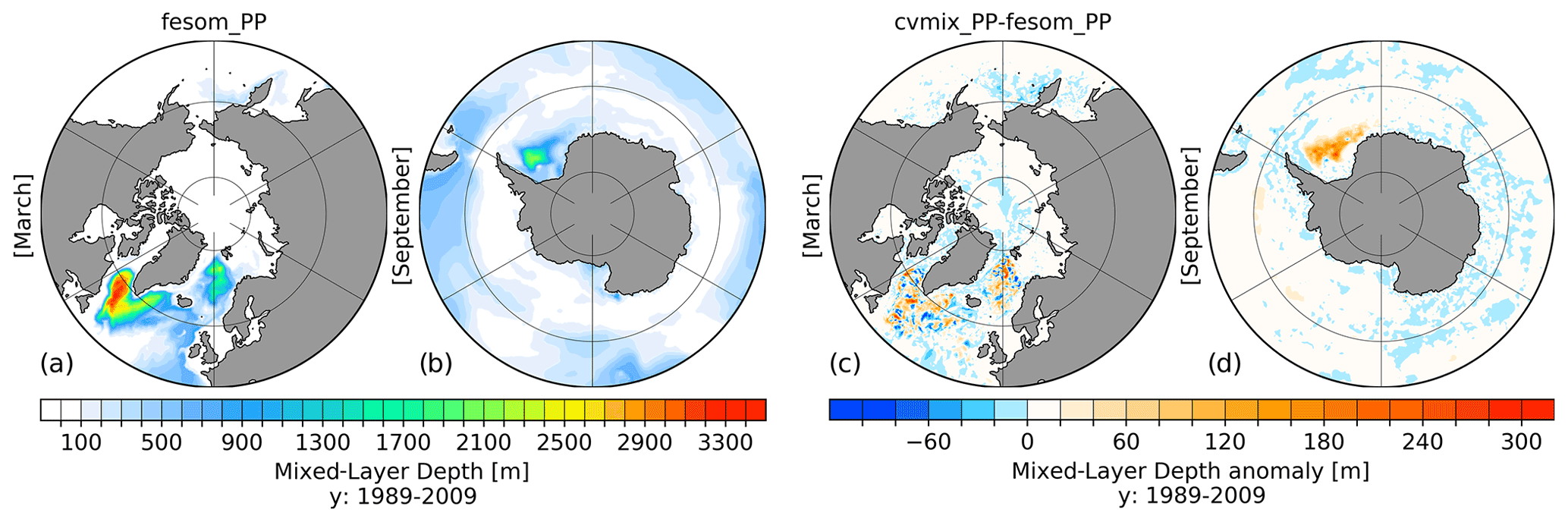
Figure 12 Northern Hemisphere March (a) and Southern Hemisphere September (b) mixed-layer depth (MLD) for fesom_PP implementation and the corresponding anomalous MLD between cvmix_PP and fesom_PP implementation (c, d) averaged for the period 1989–2009.

Figure 13 Temperature (a, e, i, m, q), salinity (b, f, j, n, r) and vertical diffusivity (c, g, k, o, s) difference between cvmix_KPP with and without TIDAL mixing of Simmons et al. (2004) and the absolute vertical diffusivity values (d, h, l, p, t) for cvmix_KPP without TIDAL mixing averaged for the period 1989 to 2009. The panels show, from top to bottom, the vertically averaged fields for the depth ranges of 0–250, 250–500, 500–1000, 1000–2000 and 2000–4000 m.

Figure 12 presents the absolute and anomalous MLD between fesom_PP and cvmix_PP. The MLD in fesom_PP in March is deep in the entire LS and in parts of the IS but slightly weaker and less spatially extended when compared to fesom_KPP (Fig. 10). The MLD in the GIN seas is very similar between fesom_PP and fesom_KPP. In the Southern Hemisphere, the September MLD in fesom_PP shows a pattern in the central Weddell Sea that is similar to that in fesom_KPP but shallower by ∼ 500 m. The MLD difference between cvmix_PP and fesom_PP in the Northern Hemisphere indicates a very heterogeneous pattern for the North Atlantic and in the Southern Hemisphere shows an up to ∼ 150 m deeper MLD in the Weddell Sea MLD for cvmix_PP compared to fesom_PP. Overall, the difference in the simulation results induced by the difference in the two implementations of mixing schemes is generally small when considering the model biases relative to observations.

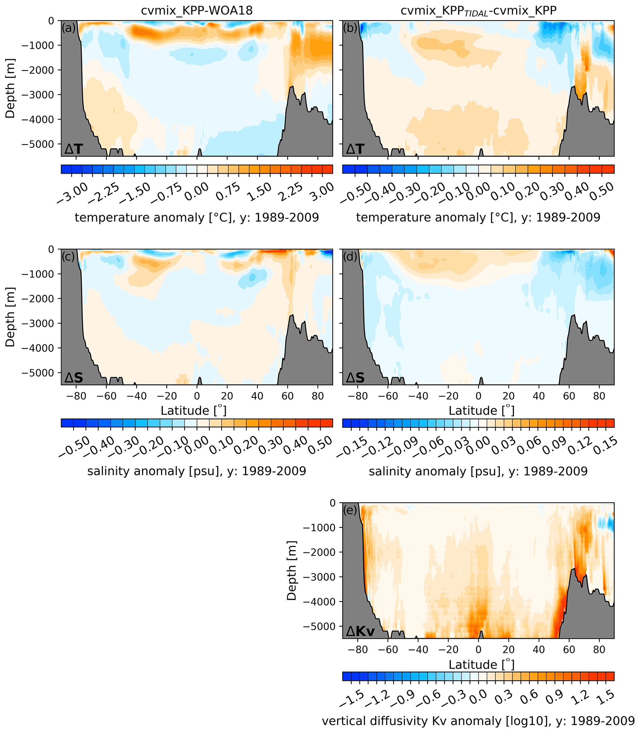
Figure 14 (a, c) Global zonal averaged climatological temperature (a) and salinity (c) bias profiles of cvmix_KPP with respect to WOA18. (b, d, e) The global zonal averaged biases of temperature (b), salinity (d) and vertical diffusivity (e) between cvmix_KPP with tidal mixing of Simmons et al. (2004) versus without it.

3.3.2 Effects of the tidal mixing parameterisation of Simmons et al. (2004)

The tidal mixing parameterisation of Simmons et al. (2004) provided by CVMix has been added to FESOM2.0. This mixing parameterisation takes into account effects from internal wave generation due to tides over rough bottom topography. The breaking of internal waves in the vicinity of topographic features excites small-scale turbulence and leads to an enhanced vertical mixing. The tidal mixing parameterisation uses a two-dimensional map of tidal energy dissipation flux due to bottom drag and energy conversion into internal waves from Jayne and St. Laurent (2001). It is transformed under consideration of a vertical redistribution function, the modelled buoyancy frequency, and a tidal dissipation efficiency and mixing efficiency into a 3D map of diapycnal tidal vertical mixing, which is added to a primary vertical mixing scheme like PP, KPP or TKE. To show the effect of the tidal mixing parameterisation, we conducted a simulation using both cvmix_KPP and the tidal vertical mixing (cvmix_KPP_TIDAL). This simulation will be compared with a control run with cvmix_KPP in which the tidal mixing is not considered. The differences in temperature (Fig. 13a, e, i, m and q), salinity (Fig. 13b, f, j, n and r) and vertical diffusivity Kv (Fig. 13c, g, k, o and s) between cvmix_KPP_TIDAL and cvmix_KPP averaged over five different depth ranges are presented in Fig. 13. Figure 13d, h, l, p and t show the cvmix_KPP Kv as a reference. The temperature anomalies of the upper three depth ranges indicate that cvmix_KPP_TIDAL is colder, especially in the marginal seas of the North Pacific, e.g. the Sea of Japan, the Sea of Okhotsk and the Bering Sea, within the branch of the Gulf Stream (GS) and North Atlantic Current (NAC), and in the GIN seas and Barents Sea. The Arctic Ocean shows a cooling anomaly for the 500–1000 and 1000–2000 m depth ranges. In the Southern Hemisphere, the entire Southern Ocean is slightly colder when including the tidal vertical mixing. The tropical and subtropical ocean indicates a slight warming for cvmix_KPP_TIDAL.

The salinity anomalies between cvmix_KPP_TIDAL and cvmix_KPP show a pattern similar to that of the temperature, with a freshening in the marginal seas of the North Pacific, GS, NAC, GIN seas, Barents Sea and the Southern Ocean. The upper depth range indicates an increase in salinity for the AO, while the subsurface depth ranges show an AO freshening when including the tidal mixing. The tropical and subtropical ocean largely shows an increase in salinity under cvmix_KPP_TIDAL.

The difference in vertical diffusivity shows an increase by an order of magnitude for cvmix_KPP_TIDAL along sloping bottom topography (e.g. the Mid-Atlantic Ridge or Indonesian region) and along the continental shelf regions that is induced by the tidal vertical mixing parameterisation. On top of that, the central AO shows a reduced vertical diffusivity by at least an order of magnitude for the 250–500, 500–1000 and 1000–2000 m depth ranges, which comes from a change in local hydrography when including the tidal vertical mixing parameterisation and the associated difference in the KPP mixing scheme.

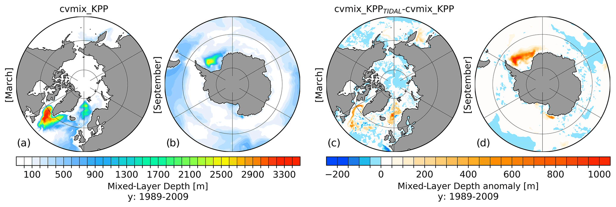
Figure 15 Northern Hemisphere March (a) and Southern Hemisphere September (b) mixed-layer depth (MLD) for cvmix_KPP without TIDAL mixing and the corresponding anomalous MLD between cvmix_KPP with minus without TIDAL mixing of Simmons et al. (2004) (c, d) averaged for the period 1989–2009.

To further understand the effect of the tidal vertical mixing, Fig. 14 shows the global zonal mean temperature and salinity differences between the case of cvmix_KPP and the WOA18 (Fig. 14a and c) and the differences between cvmix_KPP_TIDAL and cvmix_KPP (Fig. 14b and d). The temperature of cvmix_KPP shows a rather strong warming bias until 1000 m for the tropical and subtropical ocean and until ∼ 2500 m for the ocean north of 50^∘ N with respect to WOA18 (Fig. 14a). The deep ocean features small negative temperature anomalies for the tropical and subtropical ocean and slightly positive biases for the deep SO when compared to WOA18. The salinity biases of the cvmix_KPP case (Fig. 14c) indicate a more heterogeneous but nevertheless similar picture. Positive salinity biases can also be seen in the tropical and subtropical ocean until around 1000 m and until ∼ 2500 m for the ocean north of 50^∘ N. Looking at the temperature and salinity difference between cvmix_KPP_TIDAL and cvmix_KPP, it can be seen that the tidal mixing of Simmons et al. (2004) leads to a cooling and freshening of the Southern Ocean and the ocean north of 50^∘ N and a warming and salinification for the tropical and subtropical ocean until around 1500 m. The deep ocean experiences a general slight warming and freshening due to the inclusion of the tidal mixing parameterisation. In general one can summarise that the tidal mixing parameterisation of Simmons et al. (2004) helps to improve some of the biases with respect to WOA18. Figure 14e shows the global zonal averaged vertical diffusivity profiles between cvmix_KPP_TIDAL and cvmix_KPP and reveals a general strong increase in Kv along the continental slope in the Southern Ocean, in the Northern Hemisphere north of 50^∘ N and in the deep ocean interior.

To illustrate the effect of Simmons et al. (2004) tidal mixing parameterisation onto the MLD, Fig. 15 presents the Northern Hemisphere (March) (Fig. 15a) and Southern Hemisphere (September) (Fig. 15b) MLD in the case of cvmix_KPP and the difference in MLD between cvmix_KPP_TIDAL and cvmix_KPP for the Northern Hemisphere (March) (Fig. 15c) and Southern Hemisphere (September) (Fig. 15d). In the Northern Hemisphere in March, tidal mixing leads to an increase in the MLD within the boundary currents of the LS, the southern and eastern GIN seas, and in the Sea of Okhotsk. In the Southern Hemisphere (September), tidal mixing leads to a significant ∼ 1000 m increase in the Weddell Sea MLD. This significant increase originates largely from enhanced mixing of very cold surface waters along the continental slope of the Weddell Sea due to the tidal mixing parameterisation. Figure S8 in the Supplement shows the KPP OBLd for cvmix_KPP and the difference in OBLd between cvmix_KPP with and without the tidal mixing of Simmons et al. (2004). It shows that with cvmix_KPP_TIDAL the OBLd deepens, especially in the western LS.

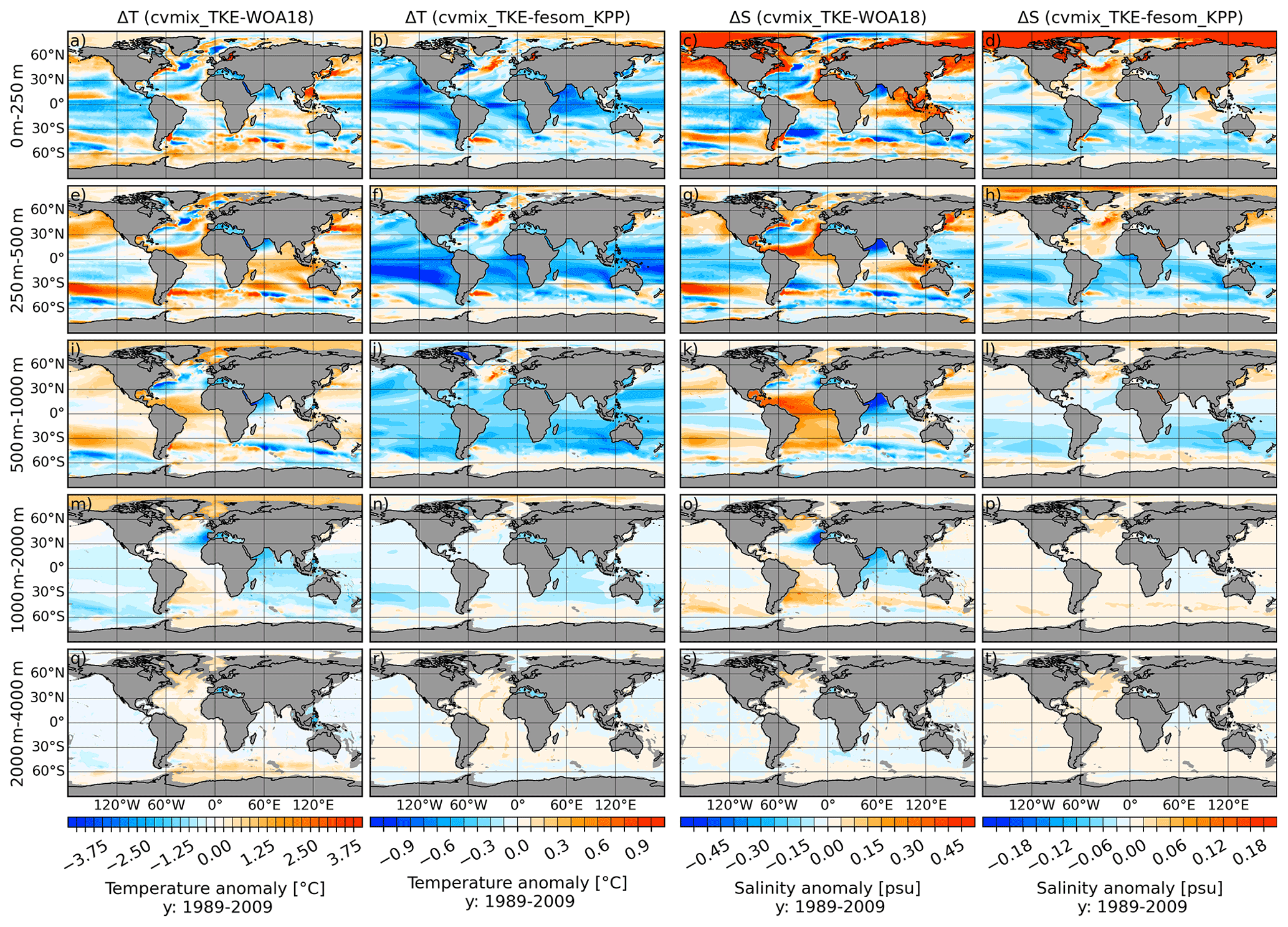
Figure 16 Temperature (a, e, i, m, q) and salinity (c, g, k, o, s) difference between cvmix_TKE and WOA18 as well as temperature (b, f, j, n, r) and salinity (d, h, l, p, t) anomaly between cvmix_TKE and fesom_KPP averaged for the period 1989 to 2009. The panels show, from top to bottom, the vertically averaged fields for the depth ranges of 0–250, 250–500, 500–1000, 1000–2000 and 2000–4000 m.

3.3.3 Effects of the turbulent kinetic energy (TKE) mixing parameterisation

More elaborate parameterisations of the vertical mixing in the ocean can be achieved by using closure schemes of turbulent kinetic energy (TKE) and the associated turbulent mixing within the mixed layer and below. One of these turbulent closure schemes is by Gaspar et al. (1990) and has been implemented via CVMix (cvmix_TKE) into FESOM2.0 based on the work of Eden et al. (2014) and Gutjahr et al. (2020). The turbulence closure scheme requires the solving of the second-order equation for TKE that is closed by connecting the vertical diffusivity with the turbulent kinetic energy and a length scale for its dissipation (Eden et al., 2014). For the background diffusivity, we do not use the latitude- and depth-dependent background diffusivity as in the previous mixing schemes. Instead, a constant minimum value of TKE is assumed that takes into account the ocean interior mixing by internal wave breaking. To understand the effect of cvmix_TKE on oceanic hydrography, Fig. 16 presents the temperature and salinity biases of cvmix_TKE with respect to WOA18 (Fig. 16a, e, i, m q and c, g, k, o, s). To relate cvmix_TKE to the other vertical mixing schemes (e.g. KPP), the temperature and salinity differences between fesom_KPP and cvmix_TKE (Fig. 16b, f, j, n, r and d, h, l, p, t) are shown as well. In general, the cvmix_TKE temperature and salinity biases with respect to WOA18 look largely very similar to the biases of fesom_KPP shown in Fig. S5 (first and third column) in terms of the spatial patterns. A closer inspection of temperature and salinity differences between cvmix_TKE and fesom_KPP (Fig. 16b, f, i, n, r and d, h, l, p, t) reveals that cvmix_TKE produces an up to 0.5 ^∘C colder ocean within the 0–250, 250–500 and 500–1000 m depth ranges in most of the ocean, a strong warming along the pathway of the NAC and the southern polar front in the South Atlantic, and small warming biases in the AO and SO. The salinity differences between cvmix_TKE and fesom_KPP indicate a salinification of the AO throughout the 0–250, 250–500 and 500–1000 m depth ranges, but salinification is most pronounced in the surface depth range. The surface saline bias largely stems from reduced mixing under sea ice, which shields the ocean from the wind stress, a large source term of TKE. Furthermore, there are positive salinity anomalies in the North Atlantic (in the pathway of the GS and NAC), North Pacific and Southern Ocean, and there are largely negative salinity anomalies in the Southern Hemisphere. The temperature and salinity differences between cvmix_TKE and fesom_KPP in the depth ranges of 1000–2000 and 2000–4000 m are rather marginal. It should be mentioned that a part of the anomalies described here could also be attributed to the different treatment of the background diffusivity. The data of fesom_KPP take a latitude- and depth-dependent value (Scholz et al., 2019), while cvmix_TKE assumes a constant value of minimum TKE on the surface (10⁻⁴ m² s⁻²) and for the interior mixing (10⁻⁶ m² s⁻²).

3.3.4 Effects of energy-consistent combination of TKE with the Internal Wave Dissipation, Energy and Mixing (IDEMIX) parameterisation

Besides the standard implementation of vertical background diffusivity in cvmix_TKE using a constant minimum value of TKE to parameterise the effect of breaking of internal waves, cvmix_TKE also allows for the usage of a more sophisticated parameterisation of internal wave breaking when combined with the IDEMIX parameterisation (Olbers and Eden, 2013; Eden et al., 2014), which describes the energy transfer from sources towards sinks of internal waves by using a radiative transfer equation of weakly interacting internal waves. The resulting dissipation of energy is then treated as a source term in the turbulent kinetic energy balance equation, leading to a more energetically consistent interpretation of the internal ocean mixing process (Eden et al., 2014; Gutjahr et al., 2020). Thereby, IDEMIX solves for the propagation of low-mode internal waves far from their generation sites, which is considered by Fox-Kemper et al. (2019) as one of the most difficult components of the internal wave energy budget. Different from the tidal mixing parameterisation of Simmons et al. (2004), which only represents the generation of internal waves by barotropic tides and their breaking at rough topography, IDEMIX considers both the internal waves due to barotropic tides and the internal waves induced by wind stress fluctuations and exiting at the base of the mixed layer (Gutjahr et al., 2020). The combination of cvmix_TKE and IDEMIX being used to improve the energetic consistency of ocean models is a rather new approach in the modelling community. It has been evaluated for stand-alone ocean models (Eden et al., 2014; Nielsen et al., 2018; Pollmann et al., 2017) and coupled models (Nielsen et al., 2019). Further, the computed TKE dissipations rates from IDEMIX have been evaluated against observational Argo float-derived dissipation rates by Pollmann et al. (2017) and have been found to be in good agreement (Gutjahr et al., 2019). In this part of the FESOM2 documentation, two FESOM2.0 simulations with cvmix_TKE, one with and one without the usage of IDEMIX, are compared to assess the effect of IDEMIX on the modelled hydrography.

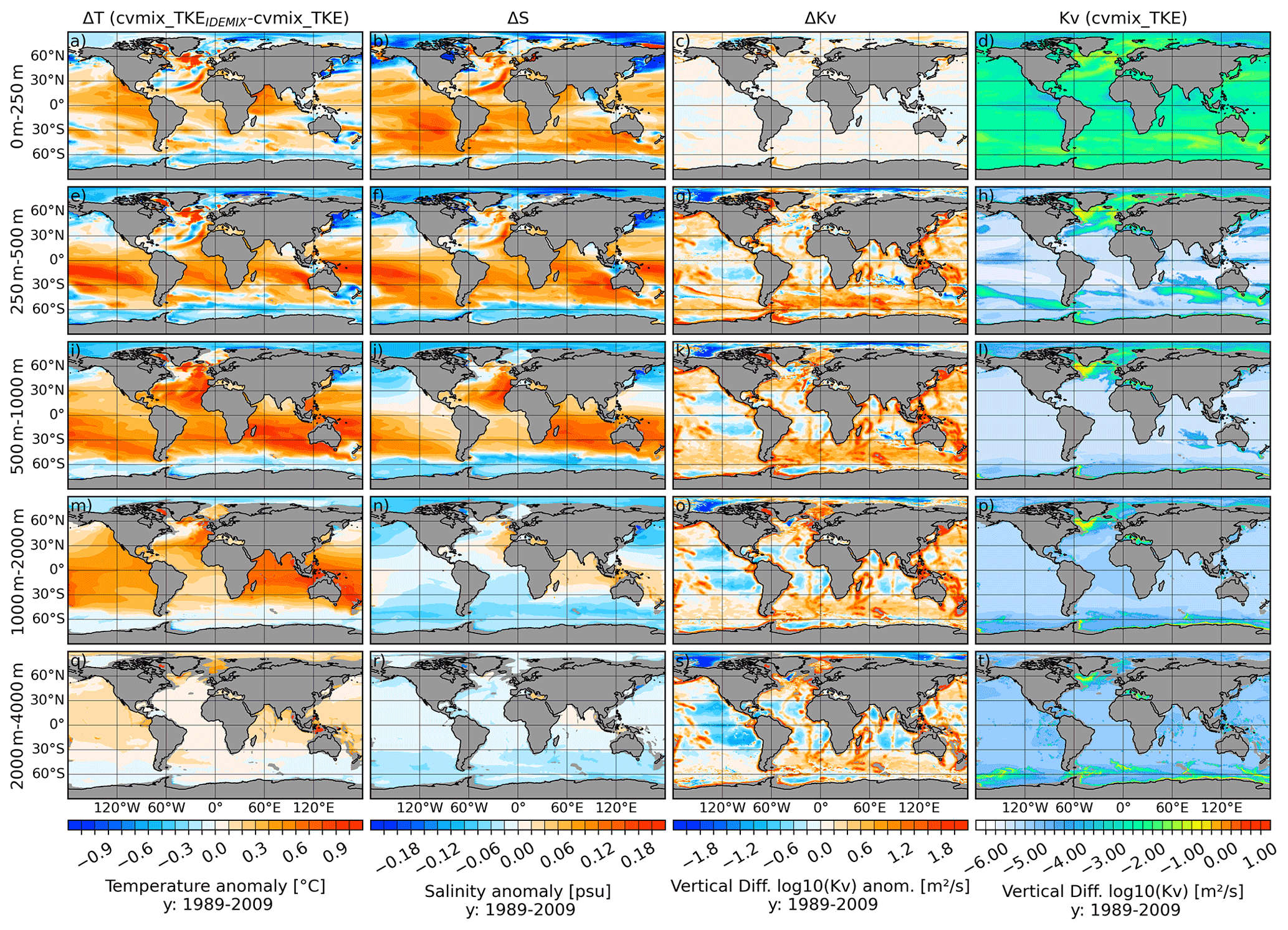
Figure 17 Temperature (a, e, i, m, q), salinity (b, f, j, n, r) and vertical diffusivity (c, g, k, o, s) difference between cvmix_TKE with and without IDEMIX and the absolute vertical diffusivity values (d, h, l, p, t) for cvmix_TKE without IDEMIX mixing averaged for the period 1989 to 2009. The panels show, from top to bottom, the vertically averaged fields for the depth ranges of 0–250, 250–500, 500–1000, 1000–2000 and 2000–4000 m.

Figure 17 presents the temperature (Fig. 17a, e, i, m and q), salinity (Fig. 17b, f, j, n and r) and vertical diffusivity (Fig17c, g, k, o and s) differences between cvmix_TKE with IDEMIX versus without it, averaged over five different depth layer ranges. As a reference, the vertical diffusivity of cvmix_TKE without IDEMIX is also shown in the Fig. 17d, h, l, p and t. The temperature differences indicate a clear warming of all equatorial and mid-latitudinal oceans and a cooling in the AO, SO and the marginal seas of the North Pacific throughout almost all the depth ranges when cvmix_TKE is used with IDEMIX. There is a particularly strong warming in the surface and subsurface depth range of the North Atlantic, in the subsurface depth range of the South Pacific and in the deeper depth ranges of the Indian Ocean. The salinity differences (Fig. 17b, f, j, n and r) have a similar spatial pattern, showing a rather strong salinification of the equatorial and mid-latitudinal global oceans and a freshening of the AO, SO and North Pacific from the surface to 500–1000 m depth range. The depth ranges below indicate a predominant general freshening almost everywhere, except for the Mediterranean outflow and Indian Ocean, which indicate a slight salinification. The differences in the vertical diffusivity between cvmix_TKE with and without IDEMIX are only very small in the upper-layer depth range. Therefore, all subsurface depth layers indicate considerable positive vertical diffusivity differences of up to two orders of magnitude, especially along all major topographic features and in the SO. This particularly shows how IDEMIX parameterises the vertical mixing due to the breaking of upward-propagating internal waves excited by barotropic tides along the ocean bottom topography but also the vertical mixing related to the internal wave breaking of downward-propagating internal waves radiated out of the mixed layer like in the SO.

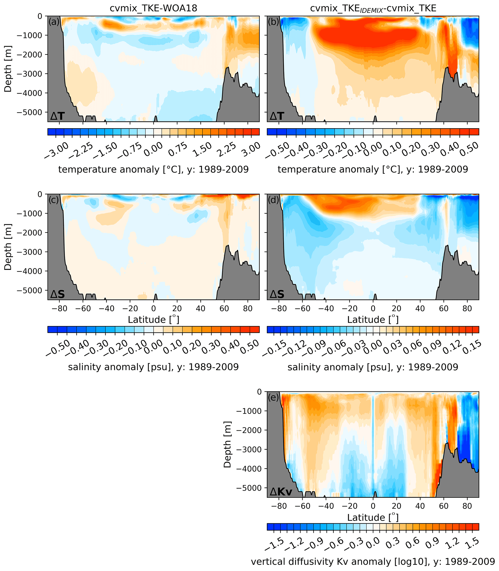
Figure 18 (a, c) Global zonal averaged climatological temperature (a) and salinity (c) bias profiles of cvmix_TKE with respect to WOA18. (b, d, e) Global zonal averaged biases of temperature (b), salinity (d) and vertical diffusivity (e) between cvmix_TKE with IDEMIX versus without it.

Figure 18 presents the global zonal mean temperature and salinity differences of cvmix_TKE with respect to the WOA18 (Fig. 18a and c), as well as the temperature, salinity and vertical diffusivity differences between cvmix_TKE_IDEMIX and cvmix_TKE (Fig. 18b, d and e). The zonal mean temperature biases of cvmix_TKE with respect to WOA18 (Fig. 18a) are positive for the upper SO, the equatorial and mid-latitudinal oceans between 500 and 1000 m, and the high-latitude ocean north of 60^∘ N where the warming bias extends nearly from the surface until a depth of ∼ 2500 m. A rather weak warming bias is also present for the very deep > 2500 m SO. General cooling biases can be seen for the equatorial and mid-latitudinal surface oceans, between a depth of ∼ 1000 and 2000 m, and for the very deep ocean. The salinity biases for cvmix_TKE (Fig. 18c) show salinities that are too high for the high-latitude ocean north of 40^∘ N and for the surface SO. Small salinity biases can be found in the equatorial and mid-latitudinal surface layers and around 40^∘ N between ∼ 1000 and 3000 m.

The temperature differences between cvmix_TKE with and without IDEMIX (Fig. 18b) show that the IDEMIX leads to a general warming of the equatorial and mid-latitudinal oceans, especially between ∼ 500 and ∼ 2000 m, but a cooling in the northern and southern high-latitude oceans. The salinity differences between cvmix_TKE with and without IDEMIX reveal a similar pattern, with an increase in salinity for the equatorial and mid-latitudinal ocean from the surface until a depth of ∼ 2000 m and a freshening bias in the same depth range for the high-latitudinal oceans and also for the entire deep ocean.

The corresponding vertical diffusivity difference is shown in Fig. 18e. In this case using IDEMIX results in an increase in vertical diffusivity along the bottom topographic slopes in the SO and north of 50^∘ N until 70^∘ N. In addition, an increase in vertical diffusivity can be observed for almost the entire upper ocean until ∼ 2000 m, with deeper-reaching positive anomalies between −60–30^∘ S and 30–50^∘ N. A reduction in the vertical diffusivity can be observed for the entire AO from the surface to bottom, for the equatorial and mid-latitudinal deep ocean > 3000 m, and for the deep (> 4000 m) SO.

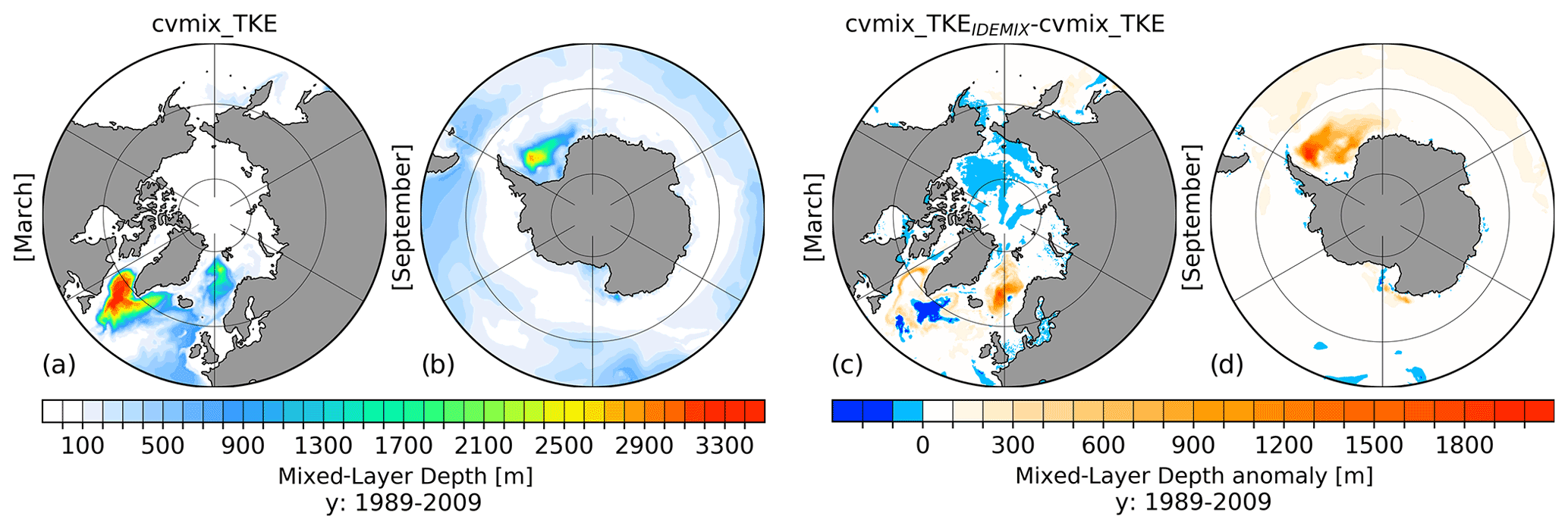
Figure 19 Northern Hemisphere March (a) and Southern Hemisphere September (b) mixed-layer depth (MLD) for cvmix_TKE without IDEMIX mixing and the corresponding anomalous MLD between cvmix_TKE with minus without IDEMIX mixing averaged for the period 1989–2009.

The effect of IDEMIX on the MLD is presented in Fig. 19, which shows the Northern Hemisphere (March, Fig. 19a) and Southern Hemisphere (September, Fig. 19b) cvmix_TKE MLD and the corresponding anomalies between cvmix_TKE with and without IDEMIX. It indicates that the use of IDEMIX leads to an increase in Northern Hemisphere MLD within the boundary currents of the LS by up to ∼ 1000 m and in the southeastern GIN seas by up to ∼ 1800 m. In the Southern Hemisphere (September), IDEMIX leads to a significant increase in the Weddell Sea MLD up to ∼ 1800 m. We observe that when using cvmix_KPP_TIDAL or cvmix_TKE_IDEMIX the model cannot maintain the upper halocline in the Weddell Sea. Hence, the warm water that remains at depth is exposed to the surface and the ocean loses heat. This can be seen clearly in Figs. 14b and 18b as blobs of negative temperature differences beneath the surface. As a consequence, the enlarged MLDs in the Weddell Sea appear. We therefore recommend combining cvmix_KPP_TIDAL or cvmix_TKE_IDEMIX with the partial bottom cell approach, which has a partly compensating effect on the stratification in the Weddell Sea (see Sect. 3.1 and Fig. S2 in the Supplement) and leads to a reduction in the MLD (Fig. S9 in the Supplement) due to improvements of the current circulation in the Weddell Sea.

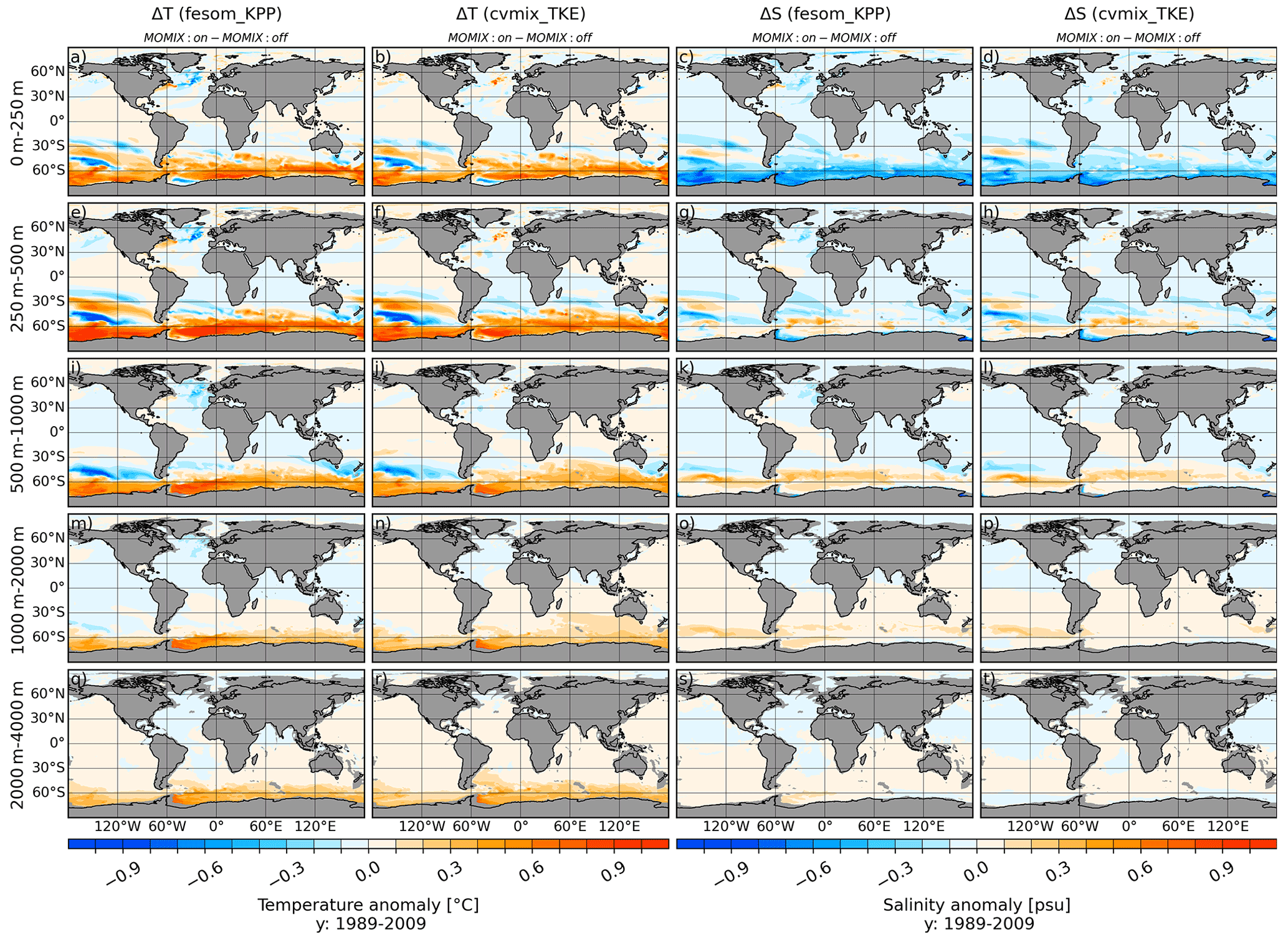
Figure 20 Temperature (a, e, i, m, q) and salinity (c, g, k, o, s) difference between fesom_KPP with and without the Monin–Obukhov vertical mixing parameterisations (MOMIX) as well as the temperature (b, f, j, n, r) and salinity (d, h, l, p, t) difference between cvmix_TKE with and without MOMIX averaged for the period 1989 to 2009. The panels show, from top to bottom, the vertically averaged fields for the depth ranges of 0–250, 250–500, 500–1000, 1000–2000 and 2000–4000 m.

3.4 Implementation of Monin–Obukhov length-dependent vertical mixing

In this section the effect of the Monin–Obukhov length vertical mixing (MOMIX) of Timmermann and Beckmann (2004) in FESOM2.0 is discussed. In an attempt to decrease climatological biases (especially in the Southern Ocean) that were otherwise prone to significant cooling and salinification (not shown), MOMIX has been implemented into FESOM2.0 as well. MOMIX serves as a parameterisation of the wind-driven mixing in the Southern Ocean and is especially effective in the melting season, which helps to reduce winter deep convection in the Weddell Sea, thus affecting the basin-wide ocean and meridional overturning circulation (Timmermann and Beckmann, 2004). MOMIX computes the Monin–Obukhov length based on heat flux, freshwater flux, wind stress, sea ice concentration and sea ice velocity following the approach of Lemke (1987), and it subsequently increases the vertical diffusivity within the Monin–Obukhov length to a value of 0.01 m² s⁻¹.

Due to its success in reducing the aforementioned mean biases, MOMIX is applied at the moment in FESOM2.0 per default south of −50^∘ S. In the following, the effects of MOMIX are discussed, based on simulation of fesom_KPP and cvmix_TKE each with and without MOMIX.

Figure 20 presents the temperature (Fig. 20a, e, i, m and q and Fig. 20b, f, j, n and r) and salinity (Fig. 20c, g, k, o and s and Fig. 20d, h, l, p and t) differences between simulations with and without MOMIX for both the fesom_KPP and cvmix_TKE schemes averaged over five different depth ranges. Using MOMIX in the Southern Ocean leads to a significant warming of up to 1 ^∘C for almost the entire Southern Ocean south of −60^∘ S throughout all considered depth ranges, except for the surface depth range of the southern Weddell Sea and subsurface southern Pacific, which exhibit cooling anomalies. The warming anomaly is slightly more pronounced for fesom_KPP than cvmix_TKE. The usage of MOMIX in the Southern Ocean leads to a warming of the Gulf Stream and to a cooling of the NAC in fesom_KPP; for cvmix_TKE this behaviour is reversed. The salinity anomalies indicate a freshening for the entire Southern Ocean surface depth range when using MOMIX, while the subsurface depth ranges predominantly indicate a slight increase in salinity, with the exception of the southern Weddell Sea 250–500 m depth range.

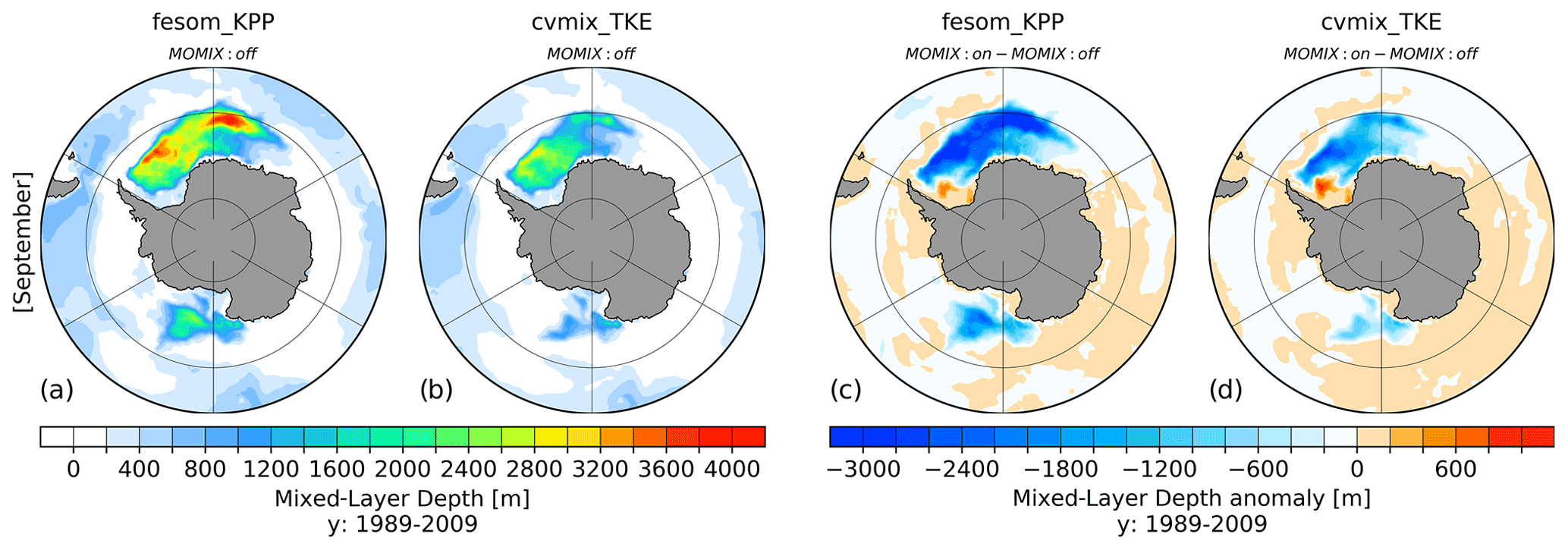
Figure 21 Southern Hemisphere September mixed-layer depth (MLD) for fesom_KPP (a) and cvmix_TKE (b) with switched-off Monin–Obukhov vertical mixing (MOMIX) parameterisation and the corresponding anomalous MLD between switched-on and switched-off MOMIX parameterisation (c, d) averaged for the period 1989–2009.

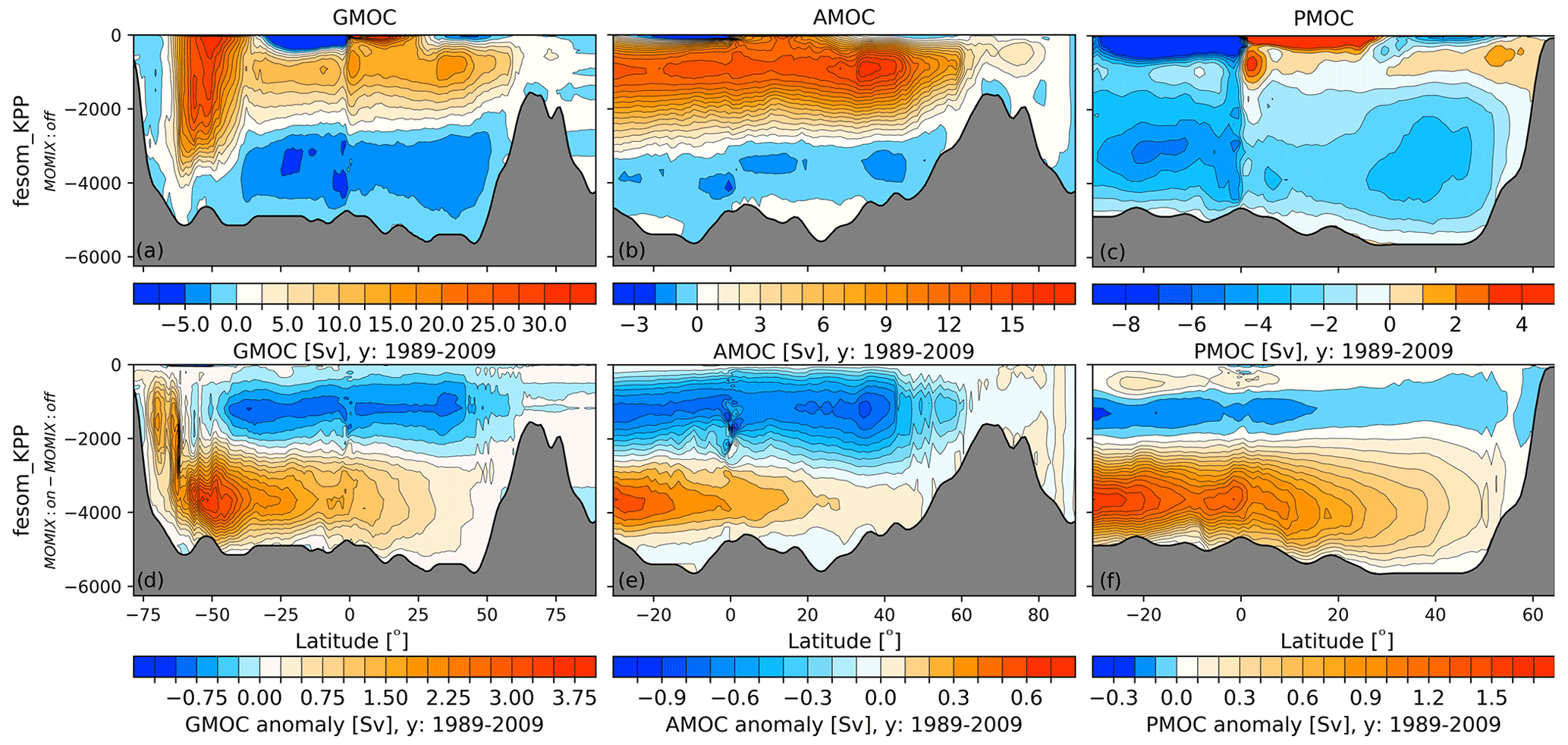
Figure 22 Absolute (a–c) and anomalous (d–f) global (GMOC, a, d), Atlantic (AMOC, b, e) and Indo-Pacific (PMOC, c, f) meridional overturning circulations averaged for the time period 1989–2009. Absolute values are shown for fesom_KPP with switched-off Monin–Obukhov vertical mixing (MOMIX) parameterisation, anomalous values show the difference between fesom_KPP with switched-on and switched-off MOMIX parameterisation.

To emphasise the effect of MOMIX on the Weddell Sea MLD, Fig. 21 presents the Southern Ocean September MLD for fesom_KPP (Fig. 21a) and cvmix_TIDAL (Fig. 21b) without MOMIX and the corresponding anomalies with minus without MOMIX (Fig. 21c and d). The MLD for fesom_KPP (Fig. 21a) and cvmix_TKE (Fig. 21b) are very large over the entire Weddell Sea and parts of the Ross Sea. The MLD values are higher and more extended with fesom_KPP than with cvmix_TKE. However, for both vertical mixing schemes without using MOMIX, the MLD values are way too high within the Weddell Sea and Ross Sea. Figure 21c and d show what happens with the Southern Ocean MLD for fesom_KPP and cvmix_TKE when MOMIX is used. Especially for fesom_KPP, MOMIX leads to a significant decrease in the MLD in almost the entire Weddell Sea of up to ∼ 3000 m, except for the southwestern Weddell Sea close to the continental shelf, which exhibits an increase in MLD. The large MLD patch in the Ross Sea also becomes strongly reduced when using MOMIX. Both fesom_KPP and cvmix_TKE face the same pattern in MLD reduction when using MOMIX, but the magnitude of the MLD decrease is larger in fesom_KPP than in cvmix_TKE.

Since MOMIX has a rather strong effect in reducing the Weddell Sea open-ocean deep-water formation it will also consequently affect the formation of Antarctic Bottom Water (AABW) and the meridional overturning circulation (MOC). Figure 22 shows the fesom_KPP global (Fig. 22a), Atlantic (Fig. 22b) and Pacific (Fig. 22c) MOC when MOMIX is switched off and its differences with the case that uses MOMIX (bottom row). It can be seen that the use of MOMIX leads to a reduction in the strength of the AABW in the Atlantic by ∼ 0.6 Sv and in the Pacific by up to ∼ 1.7 Sv on both a global and basin-wide scale. The strength of the upper AMOC cell is also reduced by ∼ 1 Sv when using MOMIX. We conclude that using MOMIX helps to alleviate the problem of large MLDs in the Weddell Sea that we addressed above. Hence, the options cvmix_KPP_TIDAL or cvmix_TKE_IDEMIX are strongly recommended for use in combination with MOMIX, which is by default only active south of −50^∘ S.

4 Discussion and conclusions

This paper describes the two new features introduced into FESOM2.0 – partial cells and embedded sea ice – and the implementation of the vertical mixing library CVMix (cvmix_PP, cvmix_KPP, cvmix_TKE, IDEMIX and cvmix_TIDAL), together with the elaboration of the effect of MOMIX. These new features expand the functionality of FESOM2.0, its applicability and its ability to be better compared to other state-of-the-art ocean general circulation models. With its model components implemented, FESOM2.0 is mature enough for practical applications and holds its leading role amongst the competition with other unstructured global ocean models.

We demonstrate the effect of using partial cells by comparing them against the full-cell approach. It is shown that partial cells lead to an improved representation of the Gulf Stream branch, with a reduction in the cold bias in the northwest corner of the North Atlantic associated with an improved NAC pathway. Further, partial cells lead to a “northwest-corner-like” meridional deflection of the NAC between −30 and −15^∘ W that is still too far east but leads to an improved representation in a rather coarse configuration that would otherwise be dominated by a rather zonal NAC. Partial cells also lead to a general speed up of the boundary currents, shown for the North Atlantic in Fig. 3.

The improvement of the NAC pathway and the speed up of the boundary currents, especially in the subpolar gyre, by using partial cells is described by a variety of publications (e.g. Barnier et al., 2006; Käse et al., 2001; Myers, 2002). Besides all of their advantages, partial cells also harbour the risk of increasing the existing biases, as can be seen in our coarse model configuration at the example of the deep Arctic warm bias, which is largely inherited from a too deep reaching Atlantic Water inflow branch. The tendency of partial cells to increase the velocity in the boundary currents leads to an enhancement of the Atlantic Water inflow to the Arctic Ocean. As the temperature in the Atlantic Water layer of the Arctic is already overestimated without using partial cells, the warm bias becomes even larger when partial cells are used. However, this is not the principle drawback of partial cells, but it is instead an issue of model tuning for the pan-Arctic region, which is part of our ongoing work (for example, evaluating different numerical schemes of momentum viscosity). In the Southern Hemisphere, using partial cells leads to a significant reduction in the otherwise rather high MLD in the Weddell Sea. Regarding the configuration used in this paper, using partial cells leads to a strengthening of the warm deep-water current (Vernet et al., 2019) that crosses the Weddell Sea interior. Thus, it enhances the local stratification (see Fig. S2 in the Supplement white arrow) and reduces vertical convection. In summary, the usage of partial cells clearly improves the general circulation within FESOM2.0, and thus the benefits outweigh the drawbacks.

The second feature that was presented is the effect of embedded sea ice versus the standard case of levitating sea ice. Embedded sea ice allows for a further step towards a more realistic and physical ocean–sea ice interaction by adding the sea ice loading to the ocean pressure. This has the potential of increasing ocean variability, especially near the sea ice edge. Our results indicate that the embedded sea ice has only a minor effect on the sea ice distribution itself. Nevertheless, the effect is the strongest for the Northern Hemisphere summer, when the sea ice edge retracts towards the Arctic Ocean interior. Embedded sea ice leads to an up to 9 % increase in the sea ice concentration in the eastern Arctic Ocean marginal seas, which also leads to an increase in the bias of the sea ice edge and to a 6 % decrease in the marginal seas of the western Arctic Ocean, which slightly reduces the sea ice extent bias there. The effect of embedded sea ice on the hydrography of the Arctic Ocean is much more significant, with an increase in temperature and salinity of up to 0.5 ^∘C and 0.1 psu, respectively, through most of the upper 1000 m. The increase in temperature and salinity is connected to a particular increase in the boundary currents, especially along the eastern boundaries of the Eurasian Basin, but also to a strengthening of the cyclonic current along the Lomonosov Ridge, which was otherwise rather weakly represented in the levitating sea ice case. The deficiencies of the Arctic Ocean current representation in our model configuration can be partially attributed to the rather coarse resolution. However, with embedded sea ice we seem to be able to at least partly counteract the effect of low resolution and improve the Arctic Ocean current structure at rather low cost. We note that embedded sea ice could also deteriorate the model results in some cases. Since the boundary currents around the Eurasian Basin get enhanced, the already existing Atlantic Water layer biases get enhanced. However, as mentioned above, this is an issue of model tuning with this coarse-resolution setup, not a drawback of embedded sea ice itself.

To further expand the functionality and comparability of FESOM2.0 we implemented the vertical mixing library CVMix and its components, which in our implementation include cvmix_PP, cvmix_KPP, cvmix_TIDAL, cvmix_TKE and cvmix_TKE+IDEMIX. At first, the vertical mixing parameterisations fesom_KPP and fesom_PP, which have been already implemented in FESOM2.0, are briefly evaluated. It is shown that fesom_PP produces slightly colder tropical and subtropical oceans but warmer polar oceans on the surface, with a largely warmer ocean below the surface layer depth range when compared to fesom_KPP. This makes fesom_KPP the preferred vertical mixing option of the two, at least in terms of mean temperature biases. In terms of salinity biases, fesom_PP performs better for the surface and subsurface AO and in the equatorial Atlantic and Indian Ocean, while otherwise fesom_KPP indicates smaller biases.

In the next instance, fesom_KPP and cvmix_KPP have been compared to each other since there are slight differences in their implementation. The difference in implementation leads to only minor differences in temperature throughout all considered depth ranges. Regarding the salinity differences, cvmix_KPP produces a considerably fresher surface AO compared to fesom_KPP, which is attributed to a reduced near-surface vertical diffusivity in cvmix_KPP that leads to an over-stabilisation of the AO halocline. This enhances the mean salinity bias in that region. In terms of vertical diffusivity, cvmix_KPP has the tendency to produce value that are up to an order of magnitude lower (especially in the very deep depth range) in the main convection areas of Labrador Sea and Greenland Sea (throughout all considered depth ranges) accompanied by increased diffusivity in the subsurface of the Arctic Ocean. The reduced diffusivity in the main convection areas is attributed to the different treatment of the shear and buoyancy difference with respect to the surface in cvmix_KPP that leads to a reduction in the local ocean boundary layer depth and to slightly reduced maximum MLD in Labrador and Greenland Sea. In contrast, the maximum MLD in the Weddell Sea becomes slightly enhanced when using cvmix_KPP over fesom_KPP.

Since the implementation of cvmix_PP and fesom_PP are also slightly different, we also compare them. Although the produced diffusivities between cvmix_PP and fesom_PP are very similar, cvmix_PP indicates a further warming and salinification in the surface and 250–500 m depth ranges except for the upwelling region in the Gulf of Guinea which indicates a cooling and freshening and the surface depth range of the Arctic Ocean where it creates a predominant freshening, when compared the fesom_PP. The MLD values indicate that cvmix_PP leads in FEOSM2.0 to a slightly stronger convection in the Weddell Sea. The differences between fesom_PP and cvmix_PP are related to the different treatment of the background coefficient for viscosity when computing the diffusivity see Pacanowski and Philander (1981).

The effect of implementing cvmix_TIDAL in combination with cvmix_KPP was further assessed. cvmix_TIDAL serves here as a resourceful way to introduce heterogeneity into the effect of tidally induced internal wave breaking that is otherwise homogenised in a constant or latitude-dependent value for the background diffusivity. Using cvmix_TIDAL clearly leads to an enhancement of the vertical diffusivity along the slopes of the bottom topography, where tidally related internal wave breaking is induced. This leads especially in the high-latitude marginal seas, e.g. the Sea of Okhotsk and Bering Sea but also the Arctic Ocean and Southern Ocean, to a decrease in temperature and salinity due to the enhanced mixing along their shelves. This enables cvmix_TIDAL to improve some of the existing local temperature and salinity biases within FESOM2.0 at rather low computational costs. However, the enhanced vertical diffusivity along the shelf of the Weddell Sea weakens the stratification and leads to a further increase in the MLD of the Weddell Sea of up to 1000 m.

Further, the implications of TKE vertical mixing parameterisation in FESOM2.0, added by Eden et al. (2014) and Gutjahr et al. (2020) to the CVMix library, were evaluated based on a comparison with fesom_KPP. It is shown that the mean temperature and salinity differences between cvmix_TKE (Fig. 17) and fesom_KPP (Fig. 9) show very similar patterns. cvmix_TKE tends to produce a generally colder tropical and extratropical ocean together with slightly warmer polar oceans when compared to fesom_KPP. The salinity differences between cvmix_TKE and fesom_KPP show that cvmix_TKE tends to produce a significantly saltier surface layer AO, revealing a much smaller salinity bias for the Arctic Ocean interior. This is largely connected to enhanced surface vertical mixing along the Arctic Ocean shelf break (not shown) within cvmix_TKE that helps to partly destabilise the AO halocline. The improvement of the Arctic Ocean hydrography when using cvmix_TKE is also found by Gutjahr et al. (2020) in the coupled ocean–atmosphere Max Planck Institute Earth System Model (MPI-ESM1.2). Further, cvmix_TKE leads to a salinity increase in the entire North Atlantic and northwestern Pacific marginal seas, while the Southern Hemisphere (except for the Southern Ocean) shows a freshening when compared to fesom_KPP. The reduced temperatures and salinities in the tropics and extratropics when using cvmix_TKE are connected to the reduced vertical mixing. However, the regions of strong vertical shear, e.g. the branch of the Gulf Stream, NAC and the Southern Ocean, show stronger vertical mixing in cvmix_TKE when compared to fesom_KPP (not shown), which is accompanied by positive temperature and salinity anomalies between cvmix_TKE and fesom_KPP.

Following the comparison of cvmix_TKE and fesom_KPP, a side-by-side comparison of cvmix_TKE with and without IDEMIX was carried out. Here IDEMIX provides an alternative formulation of the background diffusivity in cvmix_TKE using a radiative transfer equation of weakly interacting internal waves (Olbers and Eden 2013), where energy is transferred from sources of internal waves to wave sinks, such as the breaking of internal waves, which provide a source for TKE, leading to an energetically more consistent treatment of internal mixing (Eden et al., 2014). As compared to the tidal background mixing parameterisation of Simmons et al. (2004), IDEMIX allows not only for the generation of internal waves by barotropic tides interacting with marine topography but also for their propagation in the horizontal and vertical directions away from region of generation and their damping due to wave–wave interaction or interaction with the continental shelf. Further, IDEMIX allows for the excitation of internal waves at the base of the mixed layer by high-frequency wind forcing (Eden et al., 2014).

The combined TKE+IDEMIX approach has already been applied in a couple of publications (Eden et al., 2014; Nielsen et al., 2018; Gutjahr et al., 2020). It was shown in Pollmann et al. (2017) that TKE dissipation rates from the combined TKE+IDEMIX approach are comparable to dissipation rates estimated from Argo floats. In FESOM2.0, the usage of TKE+IDEMIX leads to a significant increase in the tropical and extratropical temperature and salinity and to a decrease in the high-latitude temperature and salinity over depth when compared to cases only using cvmix_TKE. These differences compensate for some of the biases in the surface and intermediate-depth ranges when IDEMIX is not used. The usage of IDEMIX leads to an enhanced heterogeneous representation of vertical mixing, especially below the mixed layer along the continental shelves and topographic slopes. However, the temperature gain for the deeper depth ranges below 1000 m seems to be strongly overestimated when using cvmix_TKE+IDEMIX, hinting at a vertical mixing in the deep ocean that is too strong. When it comes to the MLD, in the Northern Hemisphere cvmix_TKE+IDEMIX leads to a significant increase in the MLD along the Labrador Sea boundary currents and in the southern GIN seas, which can be attributed to the enhanced mixing along the continental slope of the North Atlantic and in the vicinity of the overflow regions. In the Southern Hemisphere, using IDEMIX leads to an enhancement of the vertical diffusivity along the continental slope of the Weddell Sea. This leads to an enhanced mixing of cold and salty waters, which further reduces the stratification and significantly increases the MLD of the Weddell Sea and to an overestimation of the otherwise already high MLD values.

This is in contrast to the findings of Gutjahr et al. (2020), who found that IDEMIX led to a reduction in the vertical mixing in the Weddell Sea in their coupled MPI-ESM1.2 simulation, allowing for more local stratification. One possibility to overcome the lack of performance of IDEMIX but also of cvmix_TIDAL in the Southern Ocean and Weddell Sea could be its combination with partial bottom cells, which have a tendency to significantly reduce the deep convection in the Weddell Sea. At this point further study with FESOM2.0 is also needed to analyse the different behaviour of IDEMIX that could be influenced by local resolution, coupled ocean–atmosphere feedback or just different background water mass structures. Nevertheless, the achievable energetic consistency with the combined cvmix_TKE+IDEMIX approach is an interesting feature that should find more applications in the ocean modelling community, although there is still some way to go to better understand and improve its integration.

The last part of this paper dealt with the vertical mixing parameterisation MOMIX of Timmermann and Beckmann (2004) in FESOM2.0 that helped us to overcome some major biases in the model. Since the very beginning of FESOM2.0 the model suffered from a severe cooling and salinification bias in the Southern Ocean and marginal seas around Antarctica that was accompanied by strongly overestimated MLD values and stratification in the Weddell Sea that was too weak. It is shown here that applying MOMIX south of −50^∘ S helped to significantly reduce the biases and bring the MLD depth values in the Weddell Sea into a reasonable range. MOMIX increases the vertical diffusivity within the depth range of the Monin–Obukhov mixing length. This helps the warmer and fresher surface water masses from the melting season to connect with colder and saltier subsurface water masses from the freezing season and thus increase the stratification and reduce the vertical convection. Further, the using of MOMIX in combination with fesom_KPP leads to a cooling and freshening in the branch of the NAC that seemed to be connected to a weakening of the upper AMOC cell by 1 Sv and thus to a slight reduction of the meridional heat transport. The reason why FESOM2.0 in the Southern Ocean is so dependent on MOMIX, which was not the case with FESOM1.4, needs further research. Our actual best-practice FESOM2.0 configuration uses the zstar approach with partial cells and MOMIX switched on as a default, together with fesom_KPP for the vertical mixing, although cvmix_TKE+IDEMIX shows some promising improvements, especially for Arctic applications.

To summarise, this paper is the second part of the documentation of the development of important key components of FESOM2.0 in a realistic global model configuration. We described the implementation of partial cells and embedded sea ice and their impact on the modelled hydrography. Furthermore, we briefly described the already existing vertical mixing parameterisation of fesom_KPP and fesom_PP, as well as the newly introduced mixing parameterisation of cvmix_PP, cmix_KPP, cmix_TIDAL, cvmix_TKE and cvmix_TKE+IDEMIX that came with the incorporation of the vertical mixing library CVMix into FESOM2.0.