the Creative Commons Attribution 4.0 License.
the Creative Commons Attribution 4.0 License.
 | 21 Nov 2019
Impact of model improvements on 80 m wind speeds during the second Wind Forecast Improvement Project (WFIP2)
Irina V. Djalalova
James M. Wilczak
Joseph B. Olson
Jaymes S. Kenyon
Aditya Choukulkar
Larry K. Berg
Harindra J. S. Fernando
Eric P. Grimit
Raghavendra Krishnamurthy
Julie K. Lundquist
Paytsar Muradyan
Mikhail Pekour
Yelena Pichugina
Mark T. Stoelinga
David D. Turner
During the second Wind Forecast Improvement Project (WFIP2; October 2015–March 2017, held in the Columbia River Gorge and Basin area of eastern Washington and Oregon states), several improvements to the parameterizations used in the High Resolution Rapid Refresh (HRRR – 3 km horizontal grid spacing) and the High Resolution Rapid Refresh Nest (HRRRNEST – 750 m horizontal grid spacing) numerical weather prediction (NWP) models were tested during four 6-week reforecast periods (one for each season). For these tests the models were run in control (CNT) and experimental (EXP) configurations, with the EXP configuration including all the improved parameterizations. The impacts of the experimental parameterizations on the forecast of 80 m wind speeds (wind turbine hub height) from the HRRR and HRRRNEST models are assessed, using observations collected by 19 sodars and three profiling lidars for comparison. Improvements due to the experimental physics (EXP vs. CNT runs) and those due to finer horizontal grid spacing (HRRRNEST vs. HRRR) and the combination of the two are compared, using standard bulk statistics such as mean absolute error (MAE) and mean bias error (bias). On average, the HRRR 80 m wind speed MAE is reduced by 3 %–4 % due to the experimental physics. The impact of the finer horizontal grid spacing in the CNT runs also shows a positive improvement of 5 % on MAE, which is particularly large at nighttime and during the morning transition. Lastly, the combined impact of the experimental physics and finer horizontal grid spacing produces larger improvements in the 80 m wind speed MAE, up to 7 %–8 %. The improvements are evaluated as a function of the model's initialization time, forecast horizon, time of the day, season of the year, site elevation, and meteorological phenomena. Causes of model weaknesses are identified. Finally, bias correction methods are applied to the 80 m wind speed model outputs to measure their impact on the improvements due to the removal of the systematic component of the errors.
- Article
(8742 KB) - Full-text XML
- BibTeX
- EndNote


The second Wind Forecast Improvement Project (WFIP2) took place in Oregon and Washington states from October 2015 through March 2018. This Department of Energy (DOE) and National Oceanic and Atmospheric Administration (NOAA) funded project was aimed at improving the parameterizations within the High Resolution Rapid Refresh (HRRR – 3 km horizontal grid spacing) model and its nested version (HRRRNEST – 750 m horizontal grid spacing), with the goal of increasing the forecast skill of wind turbine hub-height (80 m) wind speeds. The study area is a region of complex terrain that included a large amount of wind power generation, with more than 4.6 GW of installed capacity associated with the Bonneville Power Administration (BPA) balancing authority.
WFIP2 (Shaw et al., 2019; Wilczak et al., 2019a; Olson et al., 2019a) as well as the first WFIP (held in the US Great Plains, in 2011–2012; Wilczak et al., 2015) represent efforts to improve forecasts for the renewable energy sector. While the first WFIP was in an area with relatively flat terrain, WFIP2 took place in an area characterized by pronounced topographic features. These include the Cascade Mountains and the Columbia River Basin to the east, with the Columbia River Gorge forming a gap in the mountain range resulting in complex flow patterns in the region. Important background information regarding the project can be found in several publications: Shaw et al. (2019) presents a general overview of the project; Wilczak et al. (2019a) describes the instruments deployed for the 18-month-long campaign and the meteorological forecast challenges of the region; and Olson et al. (2019a) discusses the parameterization improvements applied to the HRRR and HRRRNEST models resulting from a better understanding of local atmospheric processes achieved by the use of the observations.
Toward the end of the campaign, a model freeze was imposed and some case studies with interesting meteorological conditions were selected to focus model improvements around. Changes to the model physical parameterizations based on model known deficiencies and findings from this campaign were then tested over these case studies and those that showed improvements were selected to become a new experimental physics suite. Finally, four 6-week periods (one for each season: “spring 2016” – 25 March–7 May 2016; “summer 2016” – 24 June–7 August 2016; “fall 2016” – 24 September–7 November 2016; and “winter 2017” – 25 December 2016–7 February 2017) were chosen to rerun the models in control (CNT) and experimental (EXP) configurations. The EXP configuration included all the modifications/improvements added to the models, while the CNT runs used the HRRR parameterization present in the NCEP operational version of the HRRR at the start of WFIP2. The four 6-week periods will be called “reforecast periods” throughout the rest of the paper, while the model reruns (HRRR CNT, HRRR EXP, HRRRNEST CNT, and HRRRNEST EXP) will be called “reforecast runs”.
Since the primary goal of WFIP2 is to advance the state of the art of wind energy forecasting in areas with complex terrain in general, and in the BPA region in particular, in this paper we use hub-height wind speed observations from sodars and profiling lidars to assess the impacts of the experimental parameterizations and finer horizontal grid spacing on the performance of the models. These instruments were chosen because they accurately measure wind speed and direction from 20 m up to a few hundred meters above ground level, which is the layer of the atmosphere most relevant for wind energy production. While in this paper improvements in bulk statistics (mean absolute error, MAE, and bias) are evaluated, a companion research article (Djalalova et al., 2019) determines the improvements using the same set of measurements and the same model runs at forecasting wind power ramp events.
The paper is organized as follows: in Sect. 2 the observational and numerical weather prediction (NWP) model datasets are described; in Sect. 3 details of the bulk statistical results are presented for 80 m wind speed MAE and bias for individual models, in terms of time of the day, model initialization time, forecast horizon, season of the year, and site elevation; in Sect. 4 improvements in the statistical results are quantified due to the experimental physics, model finer horizontal grid spacing, and a combination of the two, again as a function of the time of the day, the season of the year, and the different meteorological phenomena predominant in the area, both with and without bias correcting the model output. Section 5 presents a summary and conclusions.
2.1 Observational dataset
Various in situ, scanning, and profiling instruments were deployed and maintained by WFIP2 team partners who later provided quality controlled versions of the data. All data are available to the public from the DOE Data Archive and Portal (DAP; https://a2e.energy.gov/projects/wfip2, last access 7 November 2019). The list of instruments, deployed in nested arrays (with the outer scale of the order of 500 km and the inner scale of the order of 2 km ×2 km, see Fig. 1a of Wilczak et al., 2019a), includes three 449 MHz and eight 915 MHz radar wind profilers with radio acoustic sounding system temperature profiles, 19 sodars, five scanning lidars, five profiling lidars, four microwave radiometers, 10 microbarographs, a network of sonic anemometers, and many surface meteorological stations. An overview of the instrumentation capability and how the instruments were used for atmospheric process understanding and model validation is presented in Wilczak et al. (2019a) and Olson et al. (2019a). Also, Pichugina et al. (2019) compared a full year of wind profiles from Doppler lidars at three WFIP2 sites to the operational (at the time of their study) HRRR NCEP runs, showing how model errors varied from site to site and highlighting several aspects on where HRRR NCEP needed improvement.
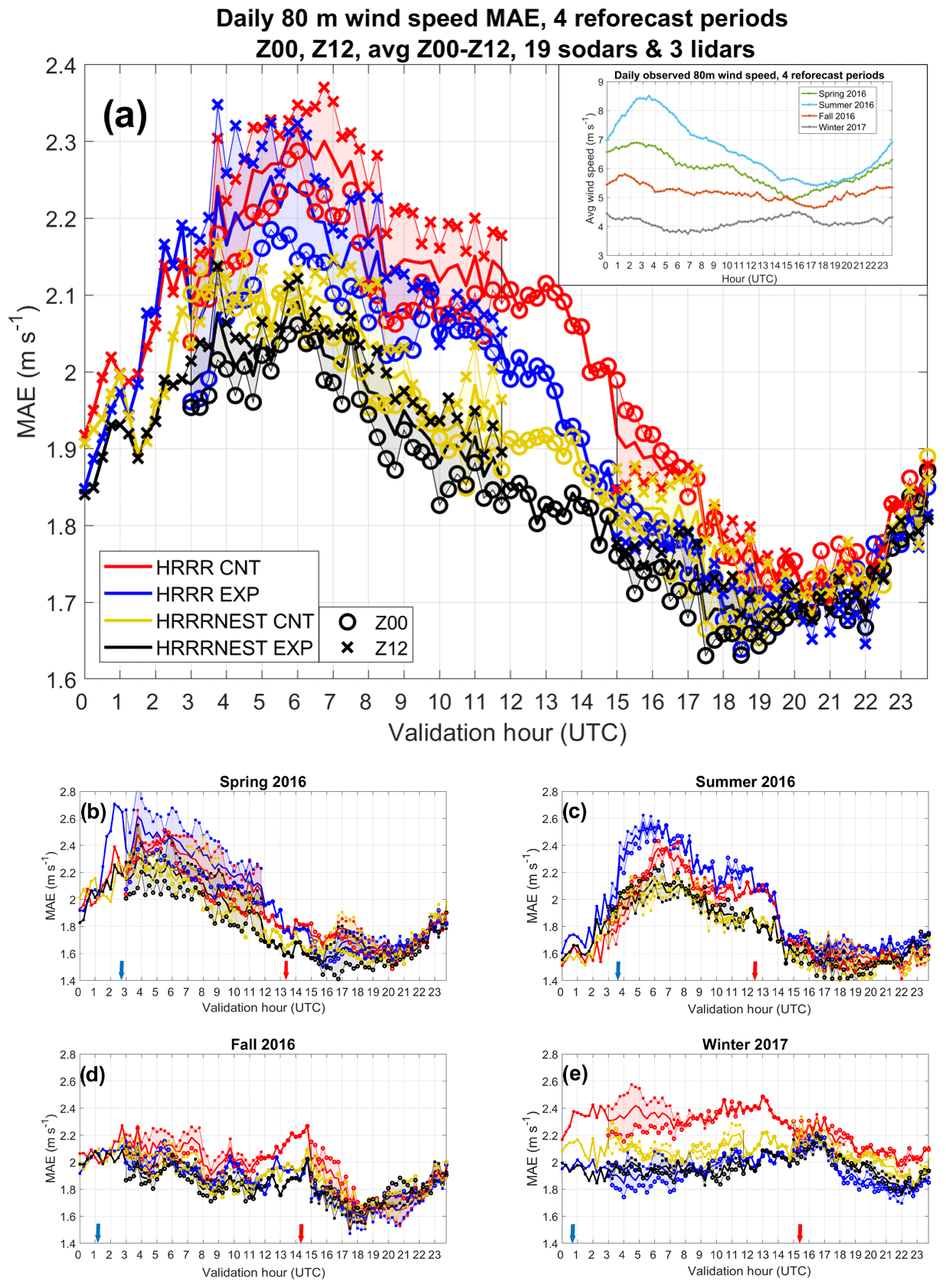
Figure 1Diurnally averaged 80 m wind speed MAEs for HRRR CNT (red curves), HRRR EXP (blue curves), HRRRNEST CNT (yellow curves), and HRRRNEST EXP (black curves). Panel (a) shows the MAEs averaged over the four reforecast periods; panel (b) are MAEs for the spring 2016 reforecast period, (c) for summer 2016, (d) for fall 2016, and (e) for winter 2017. Initialization times at 00:00 UTC (Z00) are represented by circles and at 12:00 UTC (Z12) with X's, while the solid bold lines are the averages between the Z00 and Z12 values. Red and blue arrows on the y axes represent the sunrise and sunset times, respectively. Averaged observed 80 m wind speeds are presented in the insert of panel (a) for the four reforecast periods for reference.
In the current study, data collected at 22 remote-sensing sites (19 sodars and three lidars) spanning the WFIP2 region are used, since their measurements cover the part of the atmosphere of most interest for wind energy. As measurements through the entire turbine rotor layer were not always available, we decided to focus on the 80 m level when available to avoid averaging the data over a variable depth layer of the atmosphere that could result, in some cases, in biasing the average toward values more representative of the lower part of the layer.
Some sites had a co-located sodar and lidar. In this situation the instrument with the highest data availability during the campaign was chosen. This choice led to the selection of the 19 sodars and three lidars listed in Table 1, where the latitude, longitude, elevation of the site, terrain complexity, percentage of data availability over the four reforecast periods, and the institution in charge of the instrument are also presented. The terrain complexity was computed as the standard deviation (in meters) relative to the average slope in a 6 km by 6 km area (81 points) around the site using the HRRRNEST model topography.
Table 1List of the instruments used in this study with site identification name, latitude, longitude, elevation, terrain complexity, percentage of data availability, and institution in charge (ANL: Argonne National Laboratory; ARL: Air Resources Laboratory; CU: University of Colorado; LLNL: Lawrence Livermore National Laboratory; NREL: National Renewable Energy Laboratory; PNNL: Pacific Northwest National Laboratory; UND: University of Notre Dame).
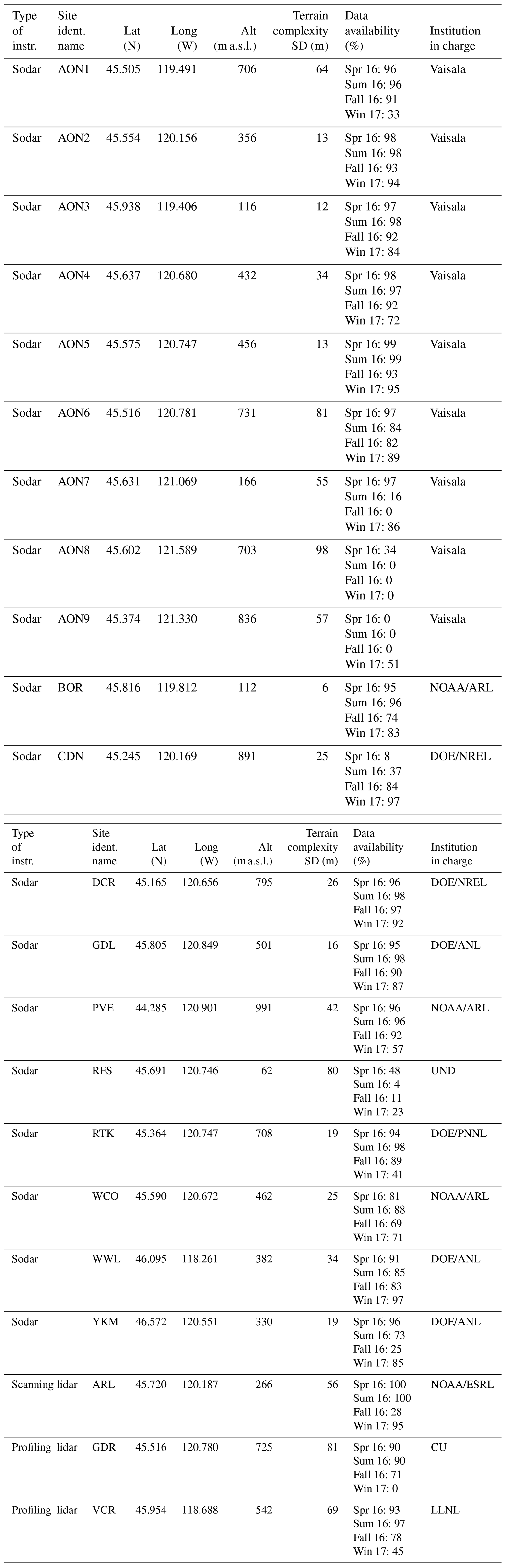
Although the focus of this study is on the 80 m wind speed statistics, we also examine the statistics of wind power generation, using a generic IEC (International Electrotechnical Commission) Class 2 power curve to convert wind speed into power. Details for the conversion from wind speed into power are given in Wilczak et al. (2019b), while Wilczak et al. (2019a) and Djalalova et al. (2019) demonstrated that the equivalent wind power generation computed from these 22 remote sensors using the abovementioned curve is representative of the actual wind power generation over the entire BPA area. The geographical location of the 19 sodars and three lidars is provided in a map later in the paper, and a more comprehensive base map of all the instruments deployed for WFIP2 is presented in Wilczak et al. (2019a).
2.2 NWP models
WFIP2 model development and improvement focused on improving forecasts in complex terrain for wind energy applications. Improvements in operational NWP models usually target extreme weather events and near-surface weather in general, with little focus on the improvement of the forecast of wind speed at hub height. Wind energy generation is especially abundant in regions of complex terrain where there are many forecasting challenges due to the complexity of the terrain-modulated flows and the feedback processes associated with them. Thus, forecast errors in hub-height wind speeds can originate from various model components. For this reason, WFIP2 model development and improvement included a number of model components: the boundary-layer and surface-layer schemes, the representation of drag associated with sub-grid-scale topography and wind farms, and the cloud–radiation interaction. Moreover, because of the complex terrain, special care had to be devoted to scaling adaptive physical parameterizations.
While the reader is referred to Olson et al. (2019a, b) for complete details on the improved model configurations, we provide a list with brief summaries of the set of model physical parameterizations and relevant numerical methods targeted for development in WFIP2.
-
Planetary boundary-layer (PBL) local mixing: mixing length revision.
The mixing length is the distance parcels are allowed to be displaced by turbulence processes, therefore depending on the size of the turbulent eddies. In the new formulation, the mixing length is independent of the height above ground and turbulent eddies are forced to be smaller than the depth of the model layer in strong stratification, thus improving maintenance of cold pools and stable boundary layers in general.
-
PBL nonlocal mixing: mass-flux scheme.
A mass-flux scheme was added to the original MYNN (Mellor–Yamada–Nakanishi–Niino) PBL scheme, making it an eddy-diffusivity mass-flux (EDMF) scheme and allowing for direct coupling of the sub-cloud convective cores and the cloud layer above. This resulted in improved coverage of shallow cumulus and improved profiles of temperature and humidity, while a smaller impact was found on low-level winds during the day.
-
Sub-grid-scale (SGS) clouds and coupling to radiation.
SGS clouds and coupling to radiation improves the downward shortwave forcing in shallow cumulus and stratocumulus conditions. The primary impact is to improve the surface energy balance, which can then more accurately drive the turbulent mixing, while a small direct impact was found on low-level winds.
-
Drag due to SGS topography.
The representation of drag due to SGS orography was added to the HRRR physics suite including surface drag due to gravity waves and form drag. While the SGS gravity wave drag acts in stable PBLs and the form drag acts for all stabilities, form drag has a smaller impact than the gravity wave drag at the high resolutions of the HRRR, and neither are active in the HRRRNEST. This addition improves the maintenance of cold pools by reducing the near-surface wind speeds (and wind speed bias), while also reducing the near-surface vertical wind shear in stable conditions.
-
Surface-layer scheme.
In the Monin–Obukhov theory the flat-terrain approximation implies that all fluxes (momentum, heat, and moisture) happen in the vertical, but this approximation becomes unrealistic in complex terrain. For this reason, the new surface-layer scalar flux algorithm now includes horizontal fluxes.
-
3-D turbulence scheme.
While typically horizontal turbulent mixing is calculated with no direct communication with the parameterized vertical mixing, the impact of horizontal fluxes can now be of similar magnitude as the vertical fluxes, improving the representation of fine-scale turbulence. The expected benefits are mostly found at sub-kilometric scales.
-
Horizontal finite differencing.
Horizontal diffusion is now performed in Cartesian space instead of terrain-following sigma coordinates. This option is a replacement to mixing along sigma coordinates, which can produce artificial vertical mixing in steep terrain. This change improves the maintenance of cold pools by no longer mixing vertically when model vertical coordinates follow steep terrain.
-
Wind farm parameterization.
A representation of wind farm drag was introduced by adopting the Weather Research and Forecasting (WRF) wind farm parameterization (Fitch et al., 2012, 2013a, b). The inclusion of this parameterization reduces a high wind speed bias within wind farms but can contribute to a slight negative wind speed bias near wind farms.
The biggest improvements in the reforecasts were found from 1, 3, and 4, which improved the representation of turbulent mixing in stable boundary layers (Olson et al., 2019a, b).
Details of the simulations used in this analysis are as follows. For the four reforecast periods (spring, summer, and fall 2016, and winter 2017), 24 h forecasts were made with the HRRR and HRRRNEST, initialized twice per day at 00:00 and 12:00 UTC, using initial conditions from the operational RAPid refresh model (RAP; Benjamin et al., 2016), with no additional data assimilation and with output available every 15 min. For simplicity, we refer to the runs initialized at 00:00 UTC as the Z00 runs and the runs initialized at 12:00 UTC as the Z12 runs. The reforecasts were run in both CNT and EXP configurations, with the EXP configuration including all the improved parameterizations. The 3 km HRRR is directly initialized from the 13 km RAP grid, so there is a spin-up period associated with the model atmosphere adjusting to the higher-resolution terrain, which typically has much higher mountain peaks and lower valleys in the HRRR relative to the RAP. This spin-up problem would be even more exaggerated if the HRRRNEST was directly initialized from the RAP model atmosphere, so to minimize this problem, we chose to allow the HRRR model atmosphere to spin-up for 3 h before we initialized the HRRRNEST from the HRRR 3 h forecast. Therefore, the HRRRNEST output runs were delayed by 3 h to ameliorate these spin-up problems so that a gap in the HRRRNEST model output exists from forecast horizon 00 to forecast horizon 02 (from 00:00 to 02:45 UTC for the Z00 initialized runs, and from 12:00 to 14:45 for the Z12 initialized runs). For this reason, in order to show meaningful comparisons between the models, we utilize only the forecast horizons 03–24 for the HRRR runs also.
For our analysis, in order to compare to the observations, the 80 m wind field is obtained from model output horizontally bilinearly interpolating to the 22 site locations using the four closest grid points and linearly vertically interpolating the two closest heights (approximately 36 and 83 m). The HRRR has relatively coarse vertical resolution, with only five full model layers below 200 m, but the middle of the third layer is very close to 80 m a.g.l., so a linear interpolation does not have a significant impact on the accuracy of the estimated 80 m wind speeds.
The observations were also averaged and interpolated in time over the 15 min model output times (most of the observations were already at a 15 min interval, but some were at a 10 min interval or less) and linearly interpolated to the 80 m level.
In this section we examine the diurnal variation in 80 m wind speed MAE and bias (model–observations) at all sites and the seasonal variation in MAE and biases from the four reforecast periods to identify the dependence of the statistics on the time of the day, model initialization time, forecast horizon, and season. The dependence on the elevation of the site is also investigated.
3.1 Statistical results as a function of the time of the day, model initialization time, forecast horizon, and season of the year
The 80 m wind speed MAEs, averaged over the 19 sodars and three lidars, show a clear diurnal pattern (Fig. 1). Each of the four reforecast runs (HRRR CNT is in red, HRRR EXP in blue, HRRRNEST CNT in yellow, and HRRRNEST EXP in black) is averaged over the four reforecast periods in panel a, while panels b–e show the four reforecast periods separately. Initialization times are represented by circles (Z00 runs) and by X's (Z12 runs), while the averages between these values are in solid, bold lines. The 80 m wind speed MAEs show a clear diurnal pattern, consistent among all model runs, with larger average MAEs during stable atmospheric conditions at nighttime (LST = UTC−8) falling mostly between 2 and 2.4 m s−1, with significantly smaller values during daytime (unstable atmospheric conditions), ranging between 1.6 and 1.8 m s−1 (panel a). For reference, the insert of Fig. 1a presents the diurnal cycle of the averaged observed 80 m wind speeds for the four reforecast periods, showing that 80 m wind speeds are higher at nighttime, particularly in summer and to a lesser extent in spring (contributing to MAE to be larger at nighttime compared to daytime) but less so in fall and winter. In addition to the larger values of MAE found at nighttime, the reforecast runs also show larger differences between the models. In contrast, during daytime not only are the MAEs smaller, but the differences between the four models reforecast runs are also smaller. Figure 1 can be used to examine the dependence of MAE on initialization time and forecast horizon. In particular, the Z00 MAEs are smaller than the Z12 MAE values for times soon after the Z00 initialization (for the first part of the day lines with circles are below lines with X's). In contrast the Z12 MAEs tend to be smaller than Z00 values for times soon after the Z12 initialization (for the second part of the day lines with X's are below lines with circles, except for HRRRNEST EXP), meaning that the MAE increases with the forecast horizon. Certainly, for each of the model reforecast runs, the time of the day is more important at determining the MAE values than the initialization time, as expected.
While on average the experimental physics and finer grid spacing lowers the MAEs over the four reforecast periods (Fig. 1a: blue, yellow, and black lines all show smaller MAEs compared to the red lines), the improvements are less consistent when looking at the four reforecast periods separately (panels b–e). In winter, the improvements are more robust, as explained in Olson et al. (2019a), due to better maintenance of cold pools, which frequently happen in this area over the winter (Whiteman et al., 2001; McCaffrey et al., 2019) and which are investigated in detail in Sect. 4.4.
The biases of the 80 m wind speed also exhibit a diurnal cycle (Fig. 2). Again, Fig. 2a shows averages of the four reforecast periods and panels b–e display the four reforecast periods separately. The diurnal trend of the bias in the HRRR CNT is evident in the red curves, with positive biases at nighttime (stable atmospheric conditions), averaging 0.7 m s−1, and negative values during daytime (unstable atmospheric conditions), down to −0.4 m s−1 (panel a). The diurnal trend for the HRRR CNT is also clear for the four reforecast periods separately (panels b–e). The HRRR EXP reforecast runs (blue curves) tend to eliminate the diurnal trend in all reforecast periods, because of the differences in the treatment of boundary-layer turbulence in unstable and stable conditions, but lower the bias significantly, leading to a negative average value of m s−1 (panel a). A possible reason for such behavior in the HRRR EXP runs can be found in the representation of drag due to SGS orography (Steeneveld et al., 2008; Tsiringakis et al., 2017) added to the HRRR physics suite. This new representation is only active in the HRRR but not in the HRRRNEST due to its finer grid spacing (Olson et al., 2019a). While the expected benefit of such improved representation of the drag is to decrease the high wind speed bias in stable conditions often found in the HRRR, the detriment in this case seems to be too large a decrease in wind speed. The addition of wind turbine drag from the wind farm parameterization also contributed to the low wind speed bias but to a lesser degree. Due to the results found in this study and in other WFIP2 related studies, ways to revisit the treatment of the drag due to sub-grid-scale orography are under consideration. Finally, the diurnal trends in the MAE and biases are smaller in the winter than in other seasons. This result could also be due to differences in the treatment of boundary-layer turbulence in unstable and stable conditions. Similar results were found by Berg et al. (2019) in their study of the sensitivity of winds simulated using the Mellor–Yamada–Nakanishi–Niino (MYNN) planetary boundary-layer parameterization in the Weather Research and Forecasting model.
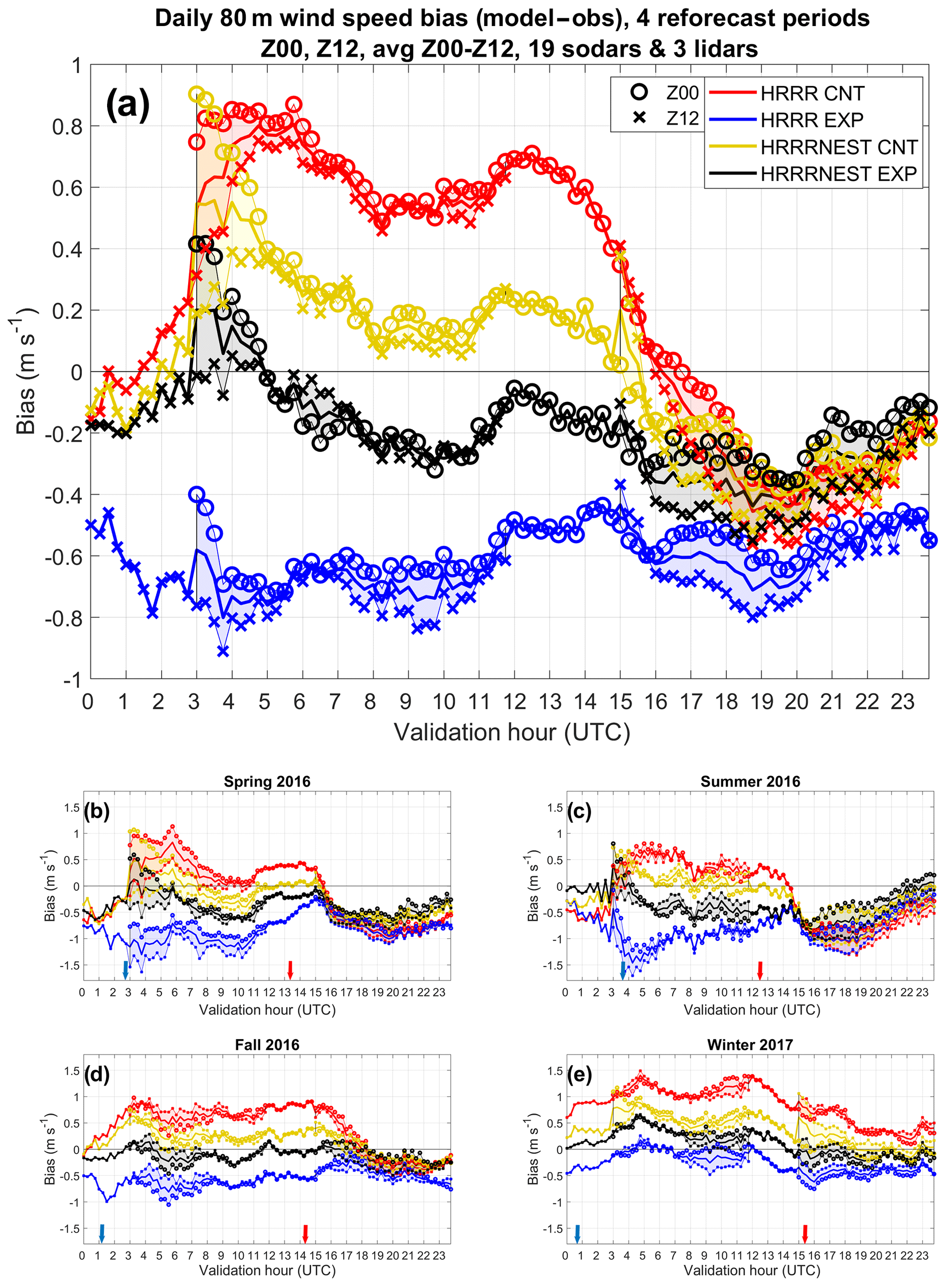
While the HRRRNEST reforecast runs (CNT in yellow and EXP in black) reduce the bias compared to their respective HRRR simulations, it is not clear yet if the HRRRNEST EXP is better than the HRRRNEST CNT or vice versa. Similarly to the MAEs, differences between the four reforecast runs are larger at nighttime and smaller during the daytime (when the biases are consistently mostly negative).
MAEs of the 80 m wind speed, presented in Fig. 3a, show that the HRRR EXP (in blue) does better than the HRRR CNT (in red) in fall and in winter but not in spring or summer. MAEs of the HRRRNEST CNT (in yellow) are better than those of the HRRR CNT (in red), and the HRRRNEST EXP (in black) is now almost always better than the other models. Biases, presented in Fig. 3b, show values in the HRRR EXP (in blue) becoming much too negative (caused by the additional orographic drag employed in the HRRR EXP) compared to the HRRR CNT (in red) in the spring, summer, and fall. Future revisions of the orographic drag in the HRRR will address this issue. The HRRRNEST EXP (black) is better than the HRRRNEST CNT (in yellow) only in the fall and winter, and again it is not clear that one of these two models has a demonstrably smaller overall bias.
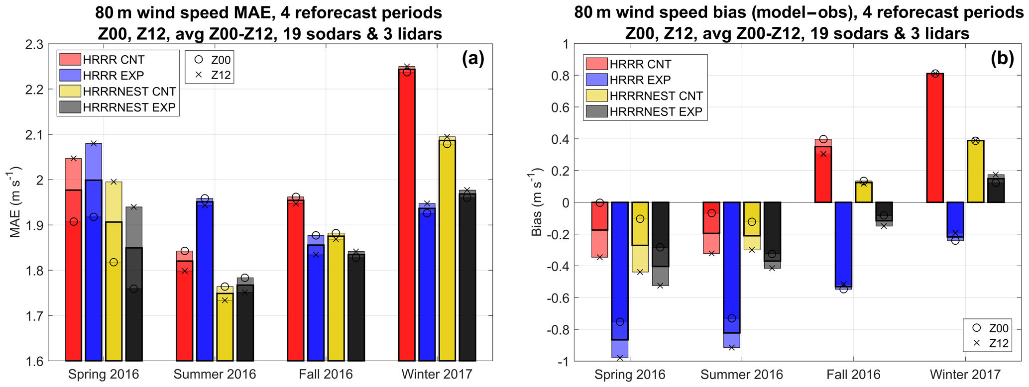
Figure 3Eighty-meter wind speed MAEs (a) and biases (b) averaged over the four reforecast periods. Initialization times are represented by circles (Z00 runs) and by X's (Z12 runs), while the solid bold lines are the averages between the Z00 and Z12 values.
The results of this section indicate that the time of the day is of primary importance in terms of MAEs and biases, while the model initialization time and the forecast horizon are of secondary importance. Consequently, the remaining statistical analysis is carried out averaging the Z00 and Z12 runs.
3.2 Statistical results as a function of the site elevation
As evident from Table 1, the 22 sites used for this analysis have very different elevations (ranging from 63 m a.s.l. at Rufus, RFS, to 991 m a.s.l. at Prineville, PVE), as well as different surrounding topographic variability. In this section, we investigate the dependence of the model error statistics on the site elevation. In Fig. 4a, b, c, and d, the results for the 80 m wind speed normalized bias, averaged over the two model initialization times, and over all forecast horizons from 03 to 24, are presented for the four reforecast periods. Sites are sorted from low to high elevation (from Rufus on the left to Prineville on the right) and biases are normalized by the averaged (observed) 80 m wind speed at each site. On the right axes of Fig. 4a, b, c, and d, we show (as dotted black lines) the averaged 80 m wind speed at each site for each reforecast period. These averages show some dependence on site elevation in fall and winter, most likely caused by cold pool events with lower wind speeds confined to the sites at lower elevation. We also note that sites at higher elevation do not have higher 80 m wind speeds than sites at lower elevation in summer and in spring. The topography of the area with the location of the sites is in Fig. 4e. The biases presented in Fig. 4 show that the diurnally and seasonally averaged biases are smaller (and often negative) at lower elevations, with a positive trend with increasing elevation. In particular, the HRRR CNT (red) has the largest positive bias at high elevations in winter which is likely due to the premature mix-out of cold pools occurring preferentially at higher elevations first, which can lead to longer periods of time with a positive wind speed bias. As in Fig. 2, HRRR EXP runs (in blue) always show the lowest bias, almost always negative, particularly at the lowest elevation sites. When not normalized by the averaged wind speed at the site (not shown) the trend was consistent with that shown in Fig. 4 but even more accentuated. In contrast, a similar analysis but for MAE normalized by the averaged 80 m wind speed at each site (not shown) did show a mostly neutral dependence on site elevation (with a slight decrease with site elevation).
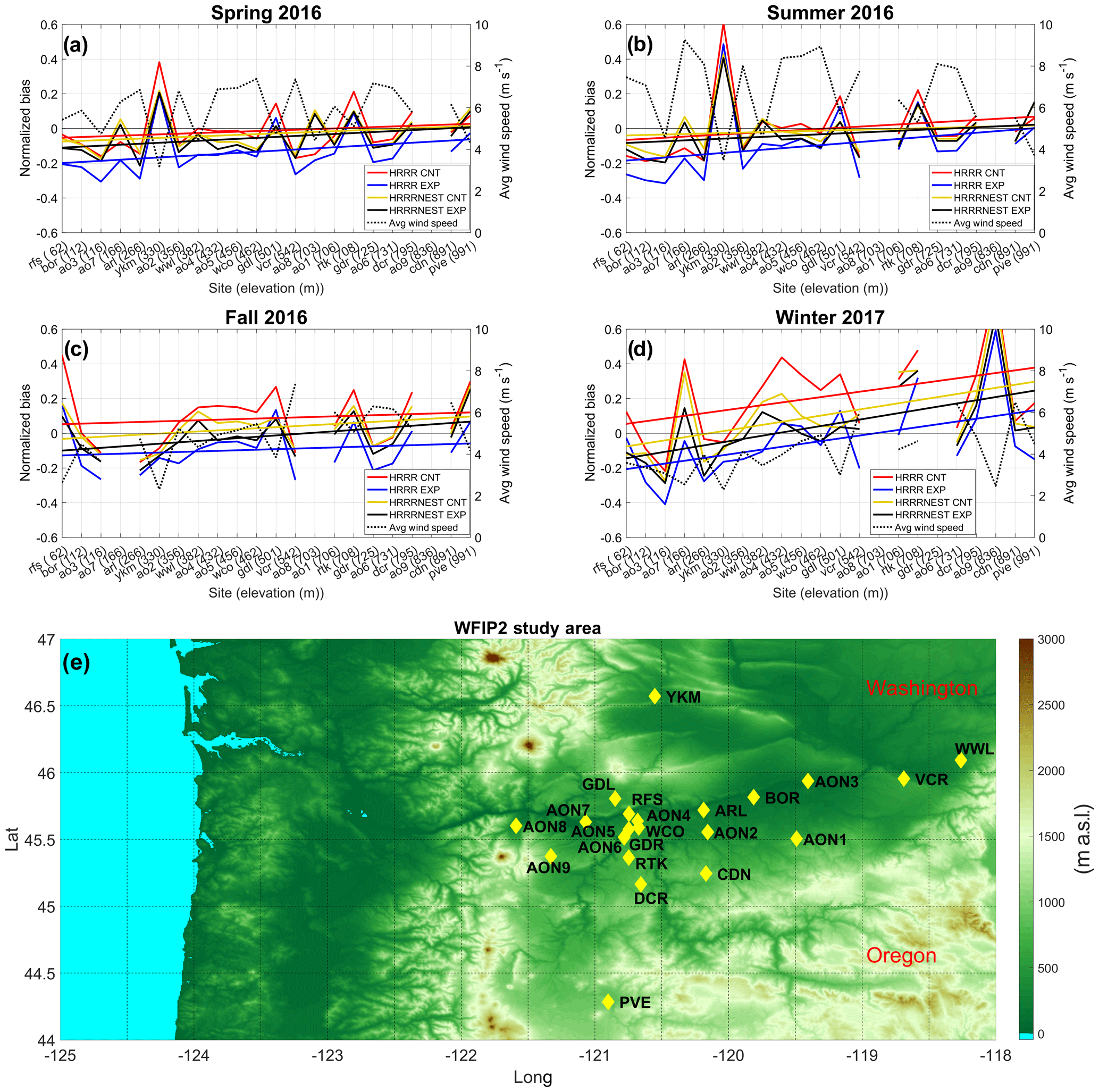
Figure 4Eighty-meter wind speed bias (model–observations) normalized by the averaged (observed, in dotted black lines) 80 m wind speed at each site for the four reforecast runs as a function of site elevation for the four reforecast periods separately: panel (a) is for the spring 2016 reforecast period, (b) for summer 2016, (c) for fall 2016 and (d) for winter 2017). Sites are sorted from low to high elevation (from Rufus at 62 m a.s.l. to Prineville at 991 m a.s.l.). Panel (e): topography of the area and location of the sites.
Although it is not clear at this point what the physical reason is for the models having a normalized bias dependent on site elevation (it may be due to the characteristics of the atmospheric phenomena predominant in this area and challenging to forecast), it is important to know that in an area of complex terrain like that of WFIP2, this dependence exists. The dependence of the bias on the elevation indicates that a post-processing bias correction of the model should be done at each site independently.
Terrain complexity is not as powerful of a predictor of model bias as site elevation. A similar analysis to that presented in Fig. 4 was performed, but sorting the sites by the complexity of the surrounding terrain (see Table 1). In this analysis (not shown) the trend of 80 m wind speed MAE and bias was not clearly defined.
In this section we examine the statistical significance and percentage improvement in the model forecast of 80 m wind speed and power. The improvements are analyzed in terms of the new physics (EXP vs. CNT runs) as well as horizontal grid spacing of the models (HRRRNEST vs. HRRR runs), first separately and then combining the impact of the two (HRRRNEST EXP vs. HRRR CNT). Finally, we evaluate the dependence of the improvements on the dominant meteorological phenomena of the area (Shaw et al., 2019), including cold pools (Whiteman et al., 2001; Zhong et al., 2001; McCaffrey et al., 2019), gap flows (Sharp and Mass, 2002, 2004), easterly flows (Neiman et al., 2018), mountain waves (Durran, 1990, 2003), topographic wakes, and convective outflows (Mueller and Carbone, 1987).
4.1 Impact of experimental physics (CNT vs. EXP runs)
The impact of the experimental physics in the HRRR runs (HRRR EXP vs. HRRR CNT) is almost always positive for wind speed and power. Percent improvement and statistical significance is shown in Fig. 5 for 80 m wind speed (a, c, e) and 80 m wind power (b, d, f). These results are obtained averaging all sites together, over the two model initialization times (forecast horizon from 03 to 24) and over the four reforecast periods. Diurnal variations in MAE (HRRR CNT in red and HRRR EXP in blue) are presented in Fig.5a and b, while panels c and d show differences between MAEs of the HRRR CNT run and MAEs of the HRRR EXP run (error bars represent the interval of this difference, where the number of points, n, is reduced by the autocorrelation of the model runs, with a 95 % confidence level chosen). Finally, the percentage MAE relative improvement of the HRRR EXP model over the HRRR CNT model (defined as 100× (MAE HRRR CNT − MAE HRRR EXP)/MAE HRRR CNT) is shown in Fig. 5e and f. Almost always positive values (improvements) are found, up to a maximum of 8 % in 80 m wind speed MAE and 10 % in 80 m wind power MAE. The impact on 80 m wind power is larger because the power increases approximately as the cubic power of the wind speed in the range of speeds between 5 and 12 m s−1 (International Electrotechnical Commission, 2007).
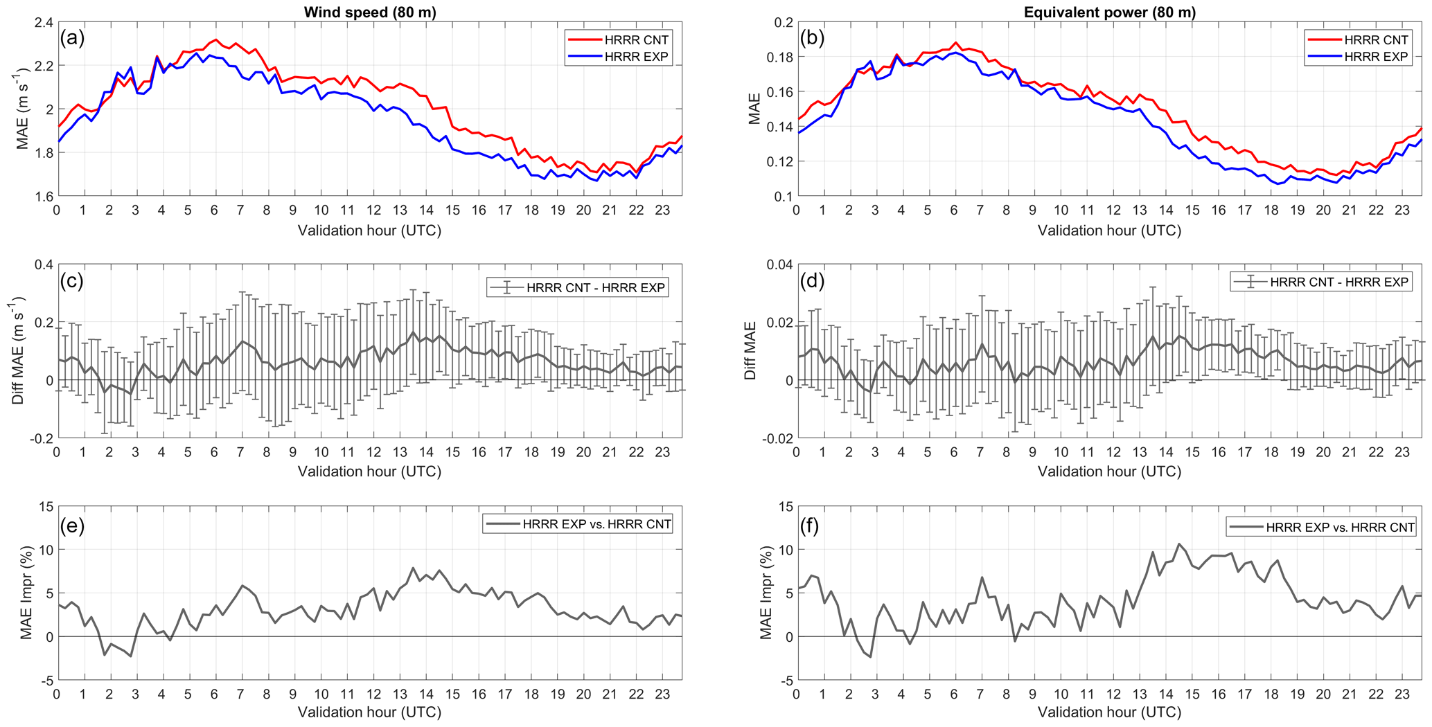
Figure 5Panels (a, c, e): HRRR EXP vs. HRRR CNT MAE for 80 m wind speed. Panels (b, d, f): as for (a, c, e), but for 80 m wind power, showing the impact of the experimental physics. Panels (a) and (b) are MAEs, (c) and (d) are differences between MAEs of the HRRR CNT run and HRRR EXP run (error bars represent the interval of the 95 % confidence level), and (e) and (f) are the percentage MAE relative improvement of the HRRR EXP model over the HRRR CNT model.
4.2 Impact of model finer horizontal grid spacing (HRRRNEST vs. HRRR)
Improvements due to finer horizontal grid spacing are larger than those due to the experimental physics. The impact of the finer horizontal grid spacing in the control runs (HRRRNEST CNT vs. HRRR CNT) is shown in Fig. 6 for 80 m wind speed (a, c, e) and 80 m wind power (b, d, f). MAE values in panels a and b are in red for the HRRR CNT runs and in yellow for the HRRRNEST CNT. In Fig. 6e and f, we see a large percentage improvement in MAE due to finer horizontal grid spacing, particularly at nighttime and during the morning transition (approximately between 01:00 and 15:00 UTC). Improvements due to finer horizontal grid spacing are larger than those due to the experimental physics in Fig. 5, with values now up to 10 % in 80 m wind speed MAE and up to 15 % in 80 m wind power MAE. The percentage improvements are smaller during daytime, when the HRRR model with larger horizontal grid spacing had lower MAE compared to nighttime.
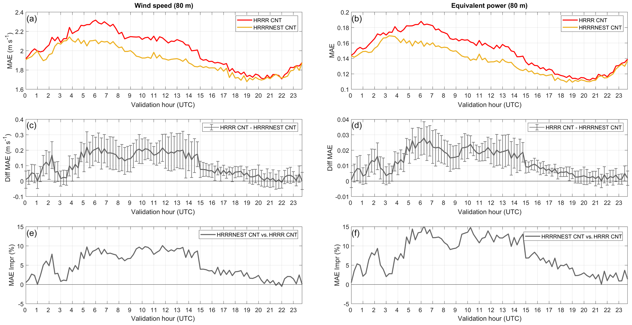
Figure 6As in Fig. 5 but for HRRRNEST CNT (in yellow) vs. HRRR CNT (in red) runs, showing the impact on 80 m wind speed MAE of finer model horizontal grid spacing.
In Fig. 7 we compare the improvements in 80 m wind speed MAE due to the experimental physics (left panels) from the HRRR (shown previously in Fig. 5) with those found in the HRRRNEST and the improvements due to finer horizontal grid spacing (right panels) from the CNT simulations (shown previously in Fig. 6) with those found in the EXP simulations. The dark blue curve shows the impact of the experimental physics on the models with larger horizontal grid spacing (HRRR EXP vs. HRRR CNT), while light blue shows the impact of the experimental physics on the models with finer horizontal grid spacing (HRRRNEST EXP vs. HRRRNEST CNT). The red curve shows the impact of finer horizontal grid spacing on the CNT runs (HRRRNEST CNT vs. HRRR CNT), while the impact of finer horizontal grid spacing on the EXP runs (HRRRNEST EXP vs. HRRR EXP) is shown in orange. When averaged over the four reforecast periods, the impact of the experimental physics (left upper panel) is quite similar between the higher and finer horizontal grid spacing models; however when considering the four reforecast periods separately (lower left smaller panels), the impact varies considerably. For example, in summer the impact of the experimental physics on the HRRRNEST is mostly neutral (light blue curve), while in the HRRR it is actually producing a negative impact (dark blue curve). In contrast, while the impact of the experimental physics is positive for both horizontal grid spacings in winter, it is very positive for the HRRR (dark blue curve). This variation could be due to changes in the physics that are grid-spacing dependent, making the impact different for HRRR and HRRRNEST. Similar considerations can be made for the improvement due to finer horizontal grid spacing (right panels). When averaged over the four reforecast periods (right upper panel) the impact of the finer horizontal grid spacing is similar between the models with different physics. However, for the winter reforecast period (lower right panel) the impact of the finer horizontal grid spacing on the EXP runs is mostly neutral (orange curve), while for the CNT runs it is clearly positive (red curve).
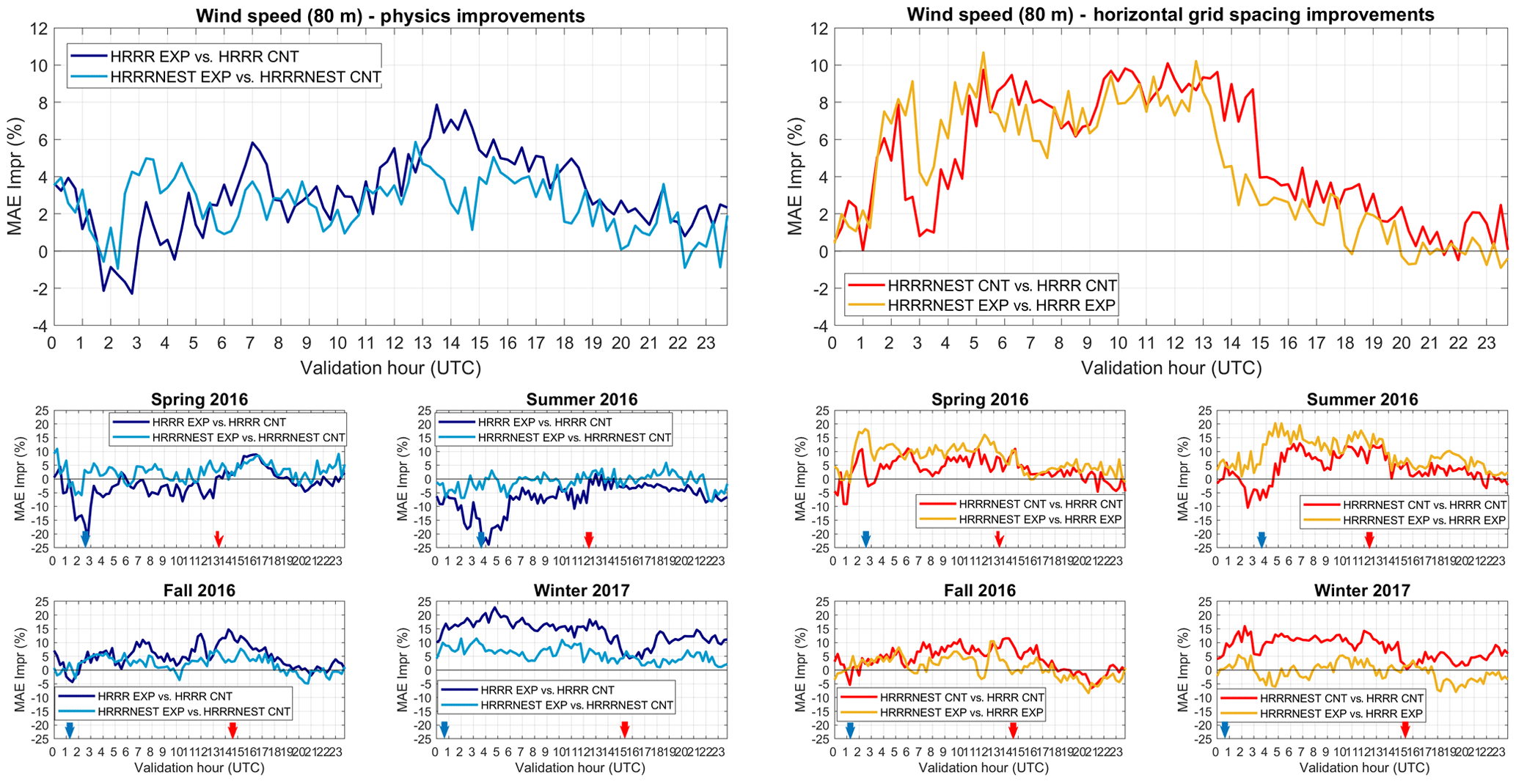
Figure 7Improvements in 80 m wind speed MAE due to the experimental physics (left panels) and finer horizontal grid spacing (right panels) for the four reforecast periods averaged together (upper panels) and for the four reforecast period separately (lower smaller panels) for all reforecast runs. Dark blue is HRRR EXP vs. HRRR CNT, light blue is HRRRNEST EXP vs. HRRRNEST CNT, red is HRRRNEST CNT vs. HRRR CNT, and orange is HRRRNEST EXP vs. HRRR EXP. Red and blue arrows on the y axes represent the sunrise and sunset times, respectively.
4.3 Impact on the statistics due to the experimental physics and finer horizontal grid spacing (HRRRNEST EXP vs. HRRR CNT)
As a final step of the analysis, the combined impact on 80 m wind speed MAE of the experimental physics and finer horizontal grid spacing, comparing the HRRRNEST EXP to HRRR CNT is shown in Fig. 8. Consistent with the results presented in the previous sections, we find that the combination of the experimental physics and finer horizontal grid spacing produces even larger improvements, always positive and up to a maximum of 14 % in the 80 m wind speed MAE (panel e) and up to a maximum of 18 % in 80 m wind power MAE (panel f). Again, larger improvements are found during the nighttime and during the morning transition, with smaller improvement found during daytime when the models had lower MAEs.
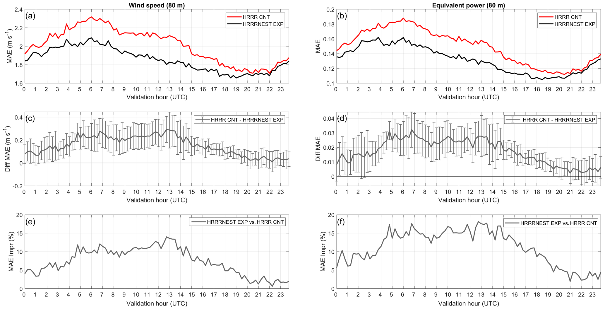
Figure 8As in Fig. 6 but for HRRRNEST EXP (in black) vs. HRRR CNT (in red) runs, showing the combined impact on 80 m wind speed MAE of the experimental physics and finer model horizontal grid spacing.
To condense the results presented in this section, a summary plot with the percentage improvements in MAE due to the experimental physics, finer horizontal grid spacing, and the combination of the two, for the four reforecast periods separately and averaged together is presented in Fig. 9 (panel a is for 80 m wind speed MAE and panel b is for 80 m wind power MAE results). For this plot the results are averaged over all sites, between the two initialization times, and over all reforecast horizons between 03 and 24. Averaged over the four reforecast periods (bars on the right side of each panel) we see improvements due to the experimental physics in the HRRR (in dark blue) and HRRRNEST (in light blue) reforecast runs, up to ∼3 % in terms of 80 m wind speed MAE and ∼4 % in terms of 80 m wind power MAE. Finer horizontal grid spacing in the CNT (in red) and EXP (in orange) reforecast runs produces improvements of up to ∼5 % for 80 m wind speed MAE and ∼7 % for 80 m wind power MAE. In gray is the improvement due to the combination of the experimental physics and finer horizontal grid spacing (HRRRNEST EXP vs. HRRR CNT), approximately 7 % for 80 m wind speed MAE and ∼11 %–12 % for 80 m wind power MAE. Considering the individual reforecast periods, in winter the improvements due to the experimental physics are very large for the HRRR, as are those due to the combination of the experimental physics and finer horizontal grid spacing (13 % for 80 m wind speed MAE and 21 % for 80 m wind power MAE). Degradations due to the changes in the physics of the HRRR (dark blue bars) are found in spring and summer, down to % for 80 m wind speed MAE and % for 80 m wind power MAE. What causes the dark blue bar in summer 2016 to be so negative? To answer this question, in the next section we investigate the improvements as a function of the different meteorological phenomena characteristic of this area (cold pools, gap flows, easterly flows, mountain waves, topographic wakes, and convective outflows).
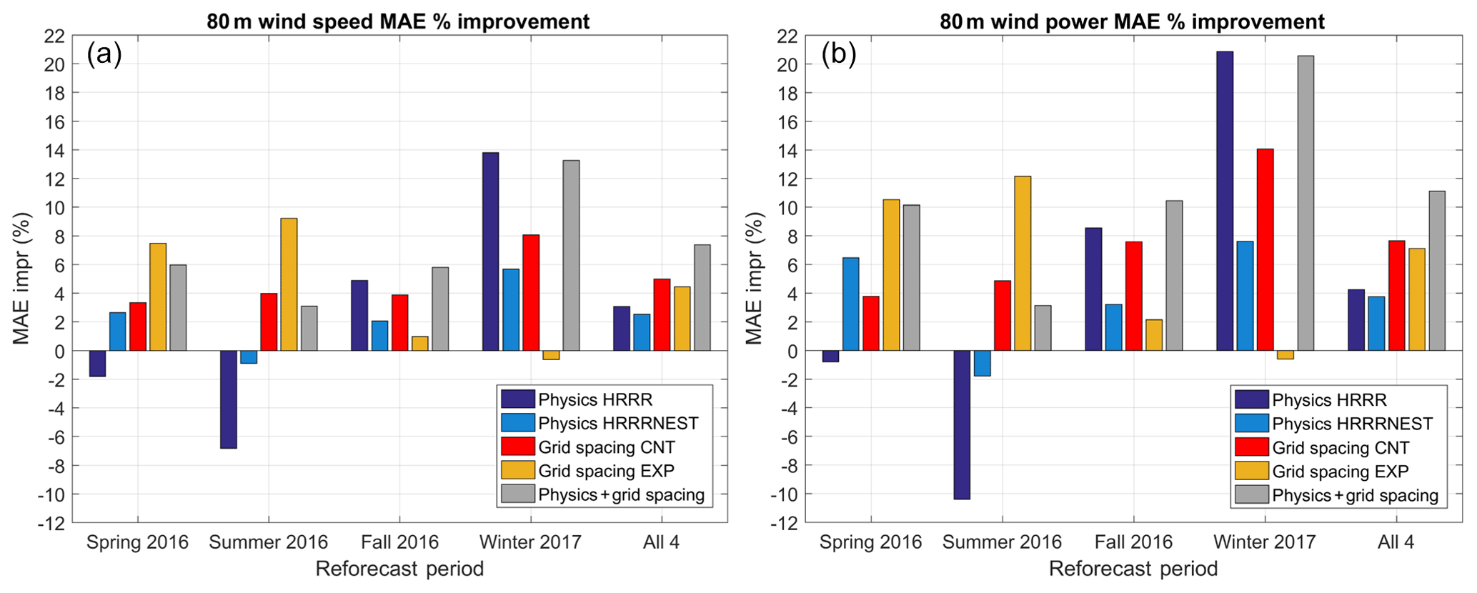
Figure 9Panel (a): percentage improvements on 80 m wind speed MAE due to the experimental physics, finer horizontal grid spacing, and the combination of the two, for the four reforecast periods separately and averaged together. Panel (b): same as (a), but for 80 m wind power MAE results.
4.4 Statistical results as a function of the different meteorological phenomena
The improvements due to the experimental physics and finer horizontal grid spacing (and to the combination of the two) as a function of the different meteorological phenomena common to this area are presented in Fig. 10. For this analysis we take advantage of the WFIP2 Event Log, which was created and updated regularly during WFIP2 by several meteorologists documenting the meteorological conditions of relevance in the area and is available on the DAP (Shaw et al., 2019). The WFIP2 meteorologists based their classification of events on WFIP2 observations and other surface observations, real-time and global model forecasts, satellite images, and local radio soundings. In the Event Log document, days and characteristics of the different meteorological phenomena were recorded, with the possibility that on some days multiple phenomena could occur at the same time. Although the categorization of the days into different meteorological phenomena involves a certain level of subjectivity, the final classification process involved weekly meetings during the field study with meteorologists on the project team, many with operational forecasting experience in this geographic area, during which a consensus was reached by the team, making us confident that other meteorologists would agree with the classifications we used. The Event Log is accessible to the public (available on the DAP, https://a2e.energy.gov/projects/wfip2, last access: 7 November 2019). For the plot in Fig. 10 the results are averaged over all sites, between the two initialization times, over all reforecast horizons between 03 and 24 and over the four reforecast periods. The number of days over which each specific phenomenon takes place is in the parentheses on the x axis label. On the far right are the improvements averaged (weighted by the number of cases) over all the different phenomena. Since on some days multiple phenomena might occur at the same time, same days can be counted multiple times in the average, which consequently is not exactly the same as that in Fig. 9. From this analysis there is no improvement in the 80 m wind speed MAE due to the modifications in the physics of the HRRR (in dark blue) for mountain waves and topographic wakes, while for the other meteorological phenomena the impact due to the experimental physics is positive. However, this figure does not tell the entire story.
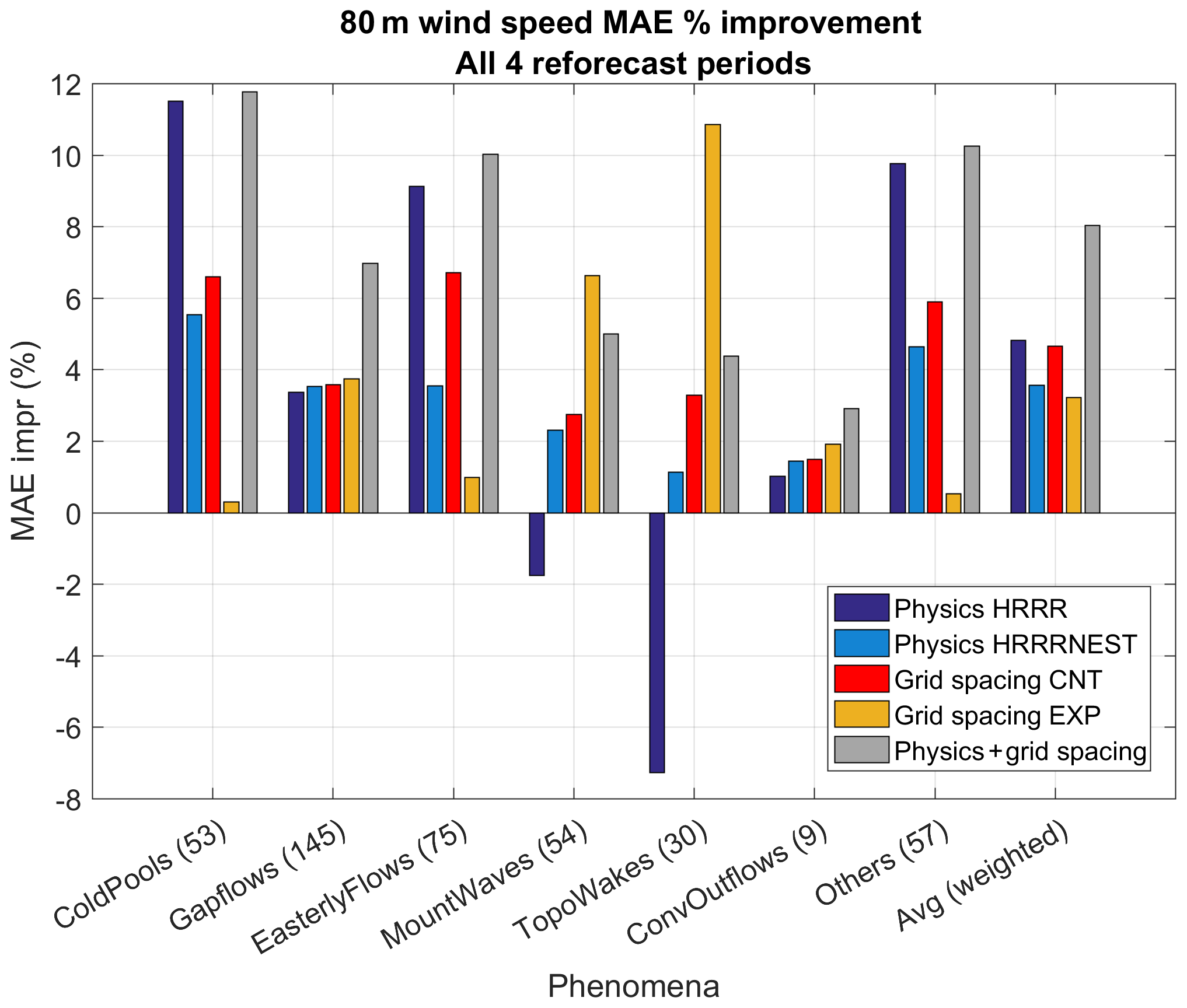
Figure 10Improvements due to the experimental physics (blue and light blue), finer horizontal grid spacing (red and orange), and the combination of the two (gray) as a function of the different meteorological phenomena common to the WFIP2 area.
As shown in Fig. 10, the number of days with gap flow events is very high (145), and if we plot the same figure separately for each of the four reforecast periods (Fig. 11), we see that the gap flow events are almost equally distributed over the four reforecast periods (34 in spring 2016, panel a; 41 in summer 2016, panel b; 38 in fall 2016, panel c; and 32 in winter 2017, panel d). For gap flow events, model performances can be different from season to season due to the fact that their nature differs from season to season (being thermally forced in summer and synoptically forced in fall and winter). Mountain wave (54 d in total) and topographic wave events (30 d in total) are also distributed over all reforecast periods. From Fig. 11 we can say that the impact of the experimental physics and finer horizontal grid spacing on 80 m wind speed MAE during gap flow, mountain waves, and topographic wake situations differs from season to season (negative in spring and summer and positive for fall and winter).
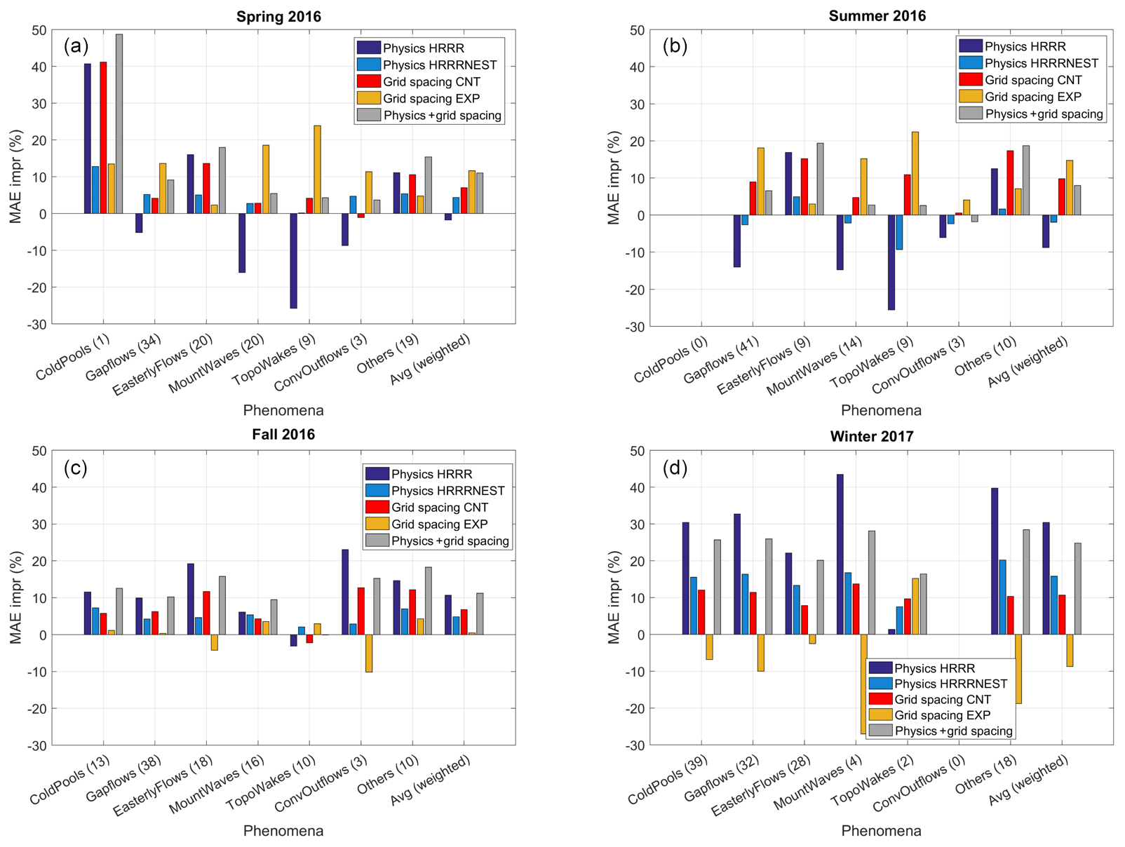
Figure 11Same as in Fig. 10, but for the four reforecast periods individually (spring, a; summer, b; fall, c; and winter, d).
Consequently, the blue bar in spring and summer extending toward negative values, visible in Fig. 9, is not only due to the negative impact of mountain wave and topographic wake days, but also to gap flow days in spring and summer (Fig. 11a, b). From Fig. 11 we also note that easterly flow is a category with a more consistent impact, always being improved by the experimental HRRR physics. Cold pool events are also consistently improved by the experimental HRRR physics; this type of event happens mostly in fall and winter (only one event is found in spring, therefore its impact cannot be considered statistically significant).
To better understand the reasons for the lack of MAE improvement in the HRRR EXP vs. HRRR CNT runs during diurnal gap flow days in summer, in Fig. 12 we present the aggregated time series of 80 m wind speed MAE (panel a) and wind speed (panel b) for the 22 sites for part of the summer reforecast period (all of the summer reforecast period shows a similar behavior). In panel b, days identified in the Event Log as experiencing gap flows are highlighted with the red shaded areas. From the time series in Fig. 12a, we see that the 80 m wind speed MAE of the HRRR EXP (blue line) is often larger than that of the HRRR CNT (red line). For almost all of the gap flow days the HRRR EXP forecasts the down-ramp too early at the end of each daily gap flow event, compared to the observations and to the HRRR CNT. Similar results were found for the spring reforecast period (not shown).
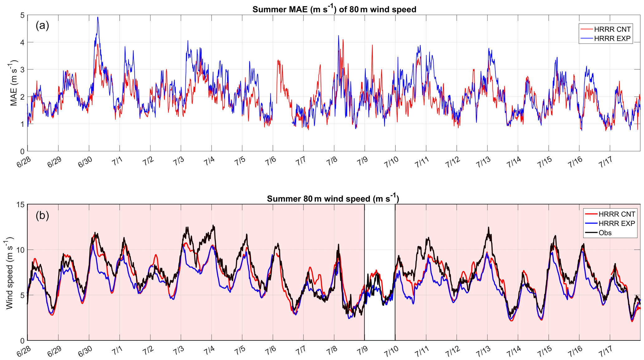
Figure 12Time series of 80 m wind speed MAE (a) and 80 m wind speed (b) for part of the summer reforecast period. HRRR CNT is in red, HRRR EXP is in blue, and observations are in black. In (b) days identified in the Event Log as experiencing gap flows are highlighted with red shading.
Although from Fig. 11 we see the experimental physics generally improves the HRRR during cold pool events, we next examine details of the when and how this improvement occurs. Figure 13 is similar to Fig. 12, but for part of the winter reforecast period. In panel b, days identified in the Event Log as experiencing cold pools are highlighted with the blue shaded areas. In the time series shown in Fig. 13a, a period when the 80 m wind speed MAE of the HRRR EXP (blue line) is larger than the HRRR CNT (red line) is highlighted with the red oval, while at a later time (inside the blue oval) the opposite is true. Differences between these cold pool events were examined using the WFIP2 real-time model observation evaluation website (http://wfip.esrl.noaa.gov/psd/programs/wfip2/, last access: 7 November 2019). This website was used through the duration of the WFIP2 field campaign for daily monitoring of model forecasts and instrument health (Wilczak et al., 2019a).
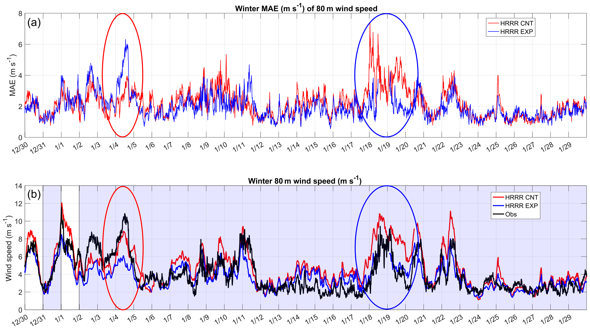
Time–height cross sections (not shown, but available from the WFIP2 real-time model observation evaluation website) of microwave radiometer temperature and winds from the radar wind profiler superimposed on radio acoustic sounding system virtual temperature at Wasco, OR, for 4 and 19 January 2017 revealed that the cold pool at the beginning of January is brought in by sustained easterly winds and has weaker stable stratification compared to the cold pool event in the second half of January, which is characterized by very low wind speeds close to the surface and more strongly stable stratification. Thus, although these periods are both listed as cold pool events, they have different atmospheric characteristics. In the first case the experimental physics in the HRRR EXP run does not help the model to outperform the HRRR CNT, while in the second case it does. A large wind speed deficit in the HRRR EXP forecast on 4 January 2017 (visible in the red oval in Fig. 13b) might occur because the HRRR EXP model has too much drag due to the SGS and/or because of the wind farm parameterization, with wind farms just upwind, east of Wasco. In contrast, on 18 January 2017, a large wind speed excess in the HRRR CNT forecast (visible in the blue oval in Fig. 13b) occurs because of (1) not enough drag in the HRRR CNT to reduce the strong winds immediately above the cold pool, (2) too much mixing at the top of the cold pool, which may be due to too large mixing lengths, and (3) “horizontal” mixing along sloped sigma coordinates, which contribute to vertical mixing. Given the very different wind and stability profile characteristics of the two cold pool events, having routinely available observations of these profiles and assimilating them into the models would likely improve their short-term forecast skill. The need for a network of ground-based profiling instruments to improve numerical weather prediction and operational forecasting is also strongly advocated by the National Research Council (2009).
4.5 Bias correction impact on the improvements
Next, we evaluate whether the improvements measured in the previous sections are mainly due to reducing the biases of the models (the systematic component of the error) or if the model improvements also address the random component of error. To this aim the model 80 m wind speed output needs to be bias corrected before the bulk statistics and the relative improvements can be computed. Several methods have been investigated in the literature to remove the systematic component of the error from model outputs. For this study, due to the nature of the 80 m wind speed biases presented in Fig. 2, two possible bias correction methods have been considered. The first one removes the mean bias from each model, at each site, and for each reforecast period separately (“mean bias”). The second method removes the mean bias from each model, at each site, for each of the reforecast periods, and for each hour of the day separately (“diurnal bias”). Since, as is clear from Fig. 2, the nature of the bias differs among the models, we examined the impacts of both of these simple bias correction methods. In Fig. 14 we present similar results to those presented Fig. 9a, but after applying the mean bias correction (Fig. 14a) and the diurnal bias correction (Fig. 14b). In both cases, the methodology used to apply the bias correction was to split the dataset into two parts, determine the bias correction on the first half and evaluate it independently on the second half of the dataset.
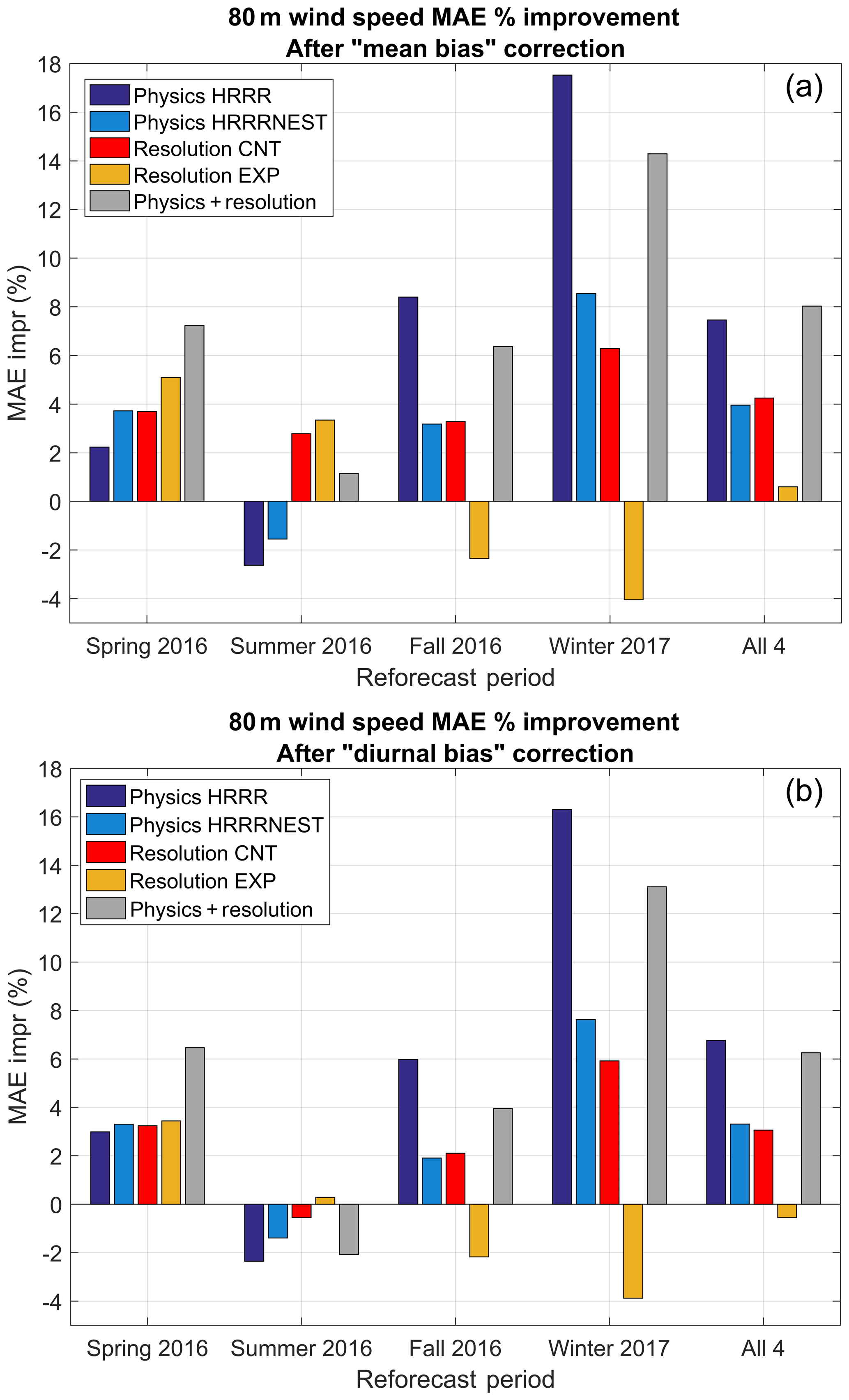
Figure 14Percentage improvements on 80 m wind speed MAE (after bias correcting the model output) due to the experimental physics, finer horizontal grid spacing, and the combination of the two for the four reforecast periods separately and averaged together. Panel (a): results using a mean bias correction; panel (b): results using a diurnal bias correction.
The mean bias correction enhances the improvement due to the experimental physics in the HRRR and HRRRNEST models (blue and light blue bars, comparing Figs. 14a to 9a). This improvement indicates that the experimental physics improves the random component of the model error, even if the experimental physics might degrade the systematic component: Fig. 3b shows that the bias of the HRRR EXP model is larger than the bias of the HRRR CNT model. In comparison, applying the diurnal bias correction (Fig. 14b) also increases the improvement due to the experimental physics (dark blue and light blue bars) over all reforecast periods and for their average, while the improvements due to finer horizontal grid spacing in the models (red and orange bars) actually decrease.
4.6 Impact of model improvements on other key meteorological variables
Although the scope of the study presented in this paper is to measure the impact of the improved model parameterizations on the forecast of 80 m wind speeds, it is important to assess what improvements, if any, were brought to other key variables in the boundary layer. Olson et al. (2019a) considered this matter when comparing HRRR (CNT and EXP) model outputs to eight 915 MHz radar wind profilers in the WFIP2 region. The 915 MHz radar wind profilers observe through the planetary boundary layer, where the MAE wind speeds were found to be reduced over all four reforecast periods, especially at night and in winter (stable atmospheric conditions), with MAE reduced by up to 0.5 m s−1 in the lower 300 m above ground level (a.g.l.), through most of the diurnal cycle. Some degradation was found in summer, for daytime, in agreement with our finding. The improvements in MAE of wind speed in the HRRRNEST runs were mostly localized in the rotor layer over which the primary goal of the campaign was focused, being much smaller over the deeper layer of the atmosphere observed by the 915 MHz radar wind profilers.
Another important variable considered by Olson et al. (2019a) was temperature, comparing the model runs to radio acoustic sounding system virtual temperature measurements. For this variable the largest improvements were found in winter, with MAE of temperatures reduced by more than 0.5 ∘C up to 400 m a.g.l. for the HRRR but half of that for the HRRRNEST.
Other key meteorological variables over which model improvements were measured by Olson et al. (2019a) were 2 m temperature and 10 m wind speed comparing the upgraded models to the previous version over the entire CONUS (CONtiguous United States) domain. For these variables RMSE and biases were improved over both the eastern and western CONUS domains, proving that model improvements in one variable were found in other variables as well.
Measurements collected by 19 sodars and three lidars during the second Wind Forecast Improvement Project (WFIP2), an 18-month field campaign in the Columbia River Gorge and Basin area, were used to validate model runs by the High Resolution Rapid Refresh (HRRR) model (3 km horizontal grid spacing) and its nested version (HRRRNEST, 750 m horizontal grid spacing).
The models were run for four 6-week reforecast periods (one for each season) in control (CNT) and experimental (EXP) configurations, where the EXP runs included new parameterizations to the HRRR and HRRRNEST physics suites (i.e., representation of wind farms and of drag associated with sub-grid-scale (SGS) topography in the HRRR), improvements to existing parameterizations (i.e., boundary-layer and surface-layer schemes, cloud–radiation interaction), and improvements to numerical methods (i.e., finite differencing of the horizontal diffusion). Results showed that:
The 80 m wind speed MAE and bias vary significantly through the diurnal cycle, with time of day being more important at determining the 80 m wind speed MAE and bias values than either the initialization time or the forecast horizon.
The HRRR EXP reforecast run reduces the diurnal trend in the bias, but results in a near constant negative bias, possibly by exaggerating the drag due to sub-grid-scale orography added to the HRRR physics suite (but not added to the HRRRNEST).
The 80 m wind speed biases have lower values (often negative) at lower elevations but increase with the site elevation. Differences in the sub-grid-scale terrain inhomogeneity did not help explain any of the bias or MAE in the results.
The experimental physics in the HRRR reduces 80 m wind speed MAE by 3 %–4 % and 80 m wind power MAE by 4 %–5 %.
Finer model horizontal grid spacing improves 80 m wind speed MAE in the control runs, particularly at nighttime and during the morning transition. Smaller improvements occur during daytime, when the larger horizontal grid spacing model had lower MAE than at nighttime. The finer horizontal grid spacing of the HRRRNEST improves 80 m wind speed MAE values up to 5 %, and 80 m wind power MAE up to 7 %–8 %.
The combined impact on 80 m wind speed MAE of the experimental physics and finer horizontal grid spacing produces an even larger reduction in MAE, averaging 7 %–8 % for 80 m wind speed and 11 %–12 % for 80 m wind power.
Improvements in MAE and bias due to the experimental physics and finer horizontal grid spacing depend on season but are almost always positive. However, in spring and summer, the experimental physics in the HRRR runs increases the 80 m wind speed MAE.
The negative impact of the experimental physics on the HRRR MAE found in spring and summer results from the degradation of the HRRR EXP on days experiencing gap flows, mountain waves, and topographic wakes and is probably due to the representation of drag in the HRRR EXP. In particular, for almost all of the summer gap flow days, the HRRR EXP predicts the down-ramps occurring at the end of the events too early.
Although cold pool forecast skill improves due to the experimental physics in the models, different types of cold pools are predicted with varying skill. If routinely available observations of wind and stability profiles were assimilated into the models, short-term forecast skill would likely improve.
Mean bias and diurnal bias corrections of the 80 m wind speed model outputs demonstrated that the experimental physics improves both the systematic and the random component of the model errors. The impacts of the different bias corrections on the improvements due to finer horizontal grid spacing in the models are mixed.
The strength of WFIP2 came from many observational scientists and model developers working closely together, steering the observational-based process understanding to guide model improvements which were later transitioned into operations. The current analysis quantifies the skill added by improvements made to the models within 4 months towards the end of WFIP2. A model freeze was then imposed so that the models could be run in EXP and CNT configurations over the four chosen reforecast periods. Since the model code freeze, three research tasks related to better simulating the low-level wind speeds have been prioritized: first the inclusion of momentum transport in the new mass-flux component of the MYNN-EDMF, second modifying the small-scale gravity wave drag to only parameterize small-amplitude gravity waves associated with sub-grid-scale terrain undulations <100 m, and third investigating the addition of a vertically distributed form drag as opposed to representing form drag only through the surface roughness length, which is probably only valid for horizontal grid spacing <1 km, where the terrain is better resolved. The impact of the first tends to increase the near-surface wind speed in the convective boundary layer, which helps to correct the low wind speed bias we measured in WFIP2. The second and the third tasks are simply meant to revise the original representation of drag in the HRRR in order to make the parameterizations more physically meaningful. All of these model components need to be investigated at a variety of model resolutions to ensure the model parameterizations successfully adapt in behavior to only represent the physical processes that are truly not well-resolved within the model.
Further improvements to the models, based on WFIP2 observations, will become part of the operational HRRR in the near future.
The operational HRRR model is not entirely open source (data assimilation/cycling scripts/etc), but updates to the model parameterizations used in the HRRR are deposited periodically to the official repository for the Advanced Research version of the Weather Research and Forecasting (WRF-ARW) model, maintained by the National Center for Atmospheric Research (NCAR), which is open source (https://github.com/wrf-model/WRF, last access: 7 November 2019). A branch from this repository was created for WFIP2 testing, based on WRF-ARWv3.9. This branch is currently stored at https://doi.org/10.5281/zenodo.3369984 (Olson and Kenyon, 2019). This branch is no longer under development and all improvements have been transferred to NCAR's official repository.
Details on the improvements applied to the HRRR and HRRRNEST parameterizations can be also found in Olson et al. (2019a).
All dataset used in this study are freely available to the public from the DOE Data Archive and Portal (DAP; https://a2e.energy.gov/projects/wfip2, last access: 7 November 2019).
Please contact the corresponding author for additional details, if needed.
LB, IVD, and JMW contributed with the data preparation, main analysis, and organization of the results in the paper. JBO and JSK worked on the improvements of the HRRR and HRRRNEST parameterizations, ran the models in CNT and EXP configurations, and contributed with useful discussions to improve the paper. AC contributed with the categorization of the atmospheric phenomena in the Event Log, with observational data, and with useful discussions to improve the paper. LKB, HJSF, EPG, RK, JKL, PM, MP, YP, MTS, and DDT contributed with observational data and with useful discussions to improve the paper.
The authors declare that they have no conflict of interest.
We thank all the people involved in WFIP2 for site selection, leases, instrument deployment and maintenance, data collection, and data quality control.
This research has been supported by the U.S. Department of Energy, Office of Energy Efficiency and Renewable Energy (grant no. DE-EE0007605) and by the NOAA/ESRL Atmospheric Science for Renewable Energy (ASRE) program. This work was authored (in part) by NREL, operated by the Alliance for Sustainable Energy, LLC, for the U.S. DOE, under contract no. DEAC36-08GO28308, with funding provided by the U.S. DOE Office of Energy Efficiency and Renewable Energy Wind Energy Technologies. Pacific Northwest National Laboratory is operated by Battelle Memorial Institute for the U.S. DOE under contract no. DEAC05-76RL01830.
This paper was edited by Klaus Gierens and reviewed by Jeffrey Freedman and one anonymous referee.
Benjamin, S. G., Weygandt, S. S., Brown, J. M., Hu, M., Alexander, C. R., Smirnova, T. G., Olson, J. B., James, E. P., Dowell, D. C., Grell, G. A.,Lin, H., Peckham, S. E., Smith, T. L., Moninger, W. R., Kenyon, J. S., and Manikin, G. S.: A North American hourly assimilation and model forecast cycle: the Rapid Refresh, Mon. Weather Rev., 144, 1669–1694, https://doi.org/10.1175/MWR-D-15-0242.1, 2016.
Berg, L. K., Liu, B., Yang, Y., Qian, Y., Olson, J., Pekour, M., Ma, P.-L., and Hou, Z.: Sensitivity of Turbine-Height Wind Speeds to Parameters in the Planetary Boundary-Layer Parametrization Used in the Weather Research and Forecasting Model: Extension to Wintertime Conditions, Bound.-Lay. Meteorol., 170, 507–518, https://doi.org/10.1007/s10546-018-0406-y, 2019.
Djalalova, I. V., Bianco, L., Akish, E., Wilczak, J. M., Olson, J. B., Kenyon, J. S., Berg, L. K., Choukulkar, A., Coulter, R., Eckman, R., Fernando, H. J. S., Grimit, E., Krishnamurthy, R., Lundquist, J. K., Muradyan, P., Pekour, M., and Stoelinga, M.: Ramp events validation during the second Wind Forecast Improvement Project (WFIP2) using the Ramp Tool and Metric (RT&M), Weather Forecasting, in preparation, 2019.
Durran, D. R.: Mountain Waves and Downslope Winds, in: Atmospheric Processes over Complex Terrain, edited by: Blumen, W., Meteorological Monographs, Vol. 23, American Meteorological Society, Boston, MA, https://doi.org/10.1007/978-1-935704-25-6_4, 1990.
Durran, D. R.: Lee Waves and Mountain Waves, Encyclopedia of Atmospheric Sciences, edited by: Holton, J. R., Pyle, J., and Curry, J. A., Elsevier: Amsterdam, The Netherlands; 1161–1169, https://doi.org/10.1016/B0-12-227090-8/00202-5, 2003.
Fitch, A. C., Olson, J. B., Lundquist, J. K., Dudhia, J., Gupta, A. K., Michalakes, J., and Barstad, I.: Local and mesoscale impacts of wind farms as parameterized in a mesoscale NWP model, Mon. Weather Rev., 140, 3017–3038, https://doi.org/10.1175/MWR-D-11-00352.1, 2012.
Fitch, A. C., Lundquist, J. K., and Olson, J. B.: Mesoscale influences of wind farms throughout a diurnal cycle, Mon. Weather Rev., 141, 2173–2198, https://doi.org/10.1175/MWR-D-12-00185.1, 2013a.
Fitch, A. C., Olson, J. B., and Lundquist, J. K.: Parameterization of wind farms in climate models, J. Climate, 26, 6439–6458, https://doi.org/10.1175/JCLI-D-12-00376.1, 2013b.
International Electrotechnical Commission: Wind turbines – Part 12-1: Power performance measurements of electricity producing wind turbines, IEC 61400-12-1, 90 pp., 2007.
McCaffrey, K, Wilczak, J. M., Bianco, L., Grimit, E., Sharp, J., Banta, R., Friedrich, K., Fernando, H. J. S., Krishnamurthy, R., Leo, L., and Muradyan, P.: Identification and characterization of persistent cold pool events from temperature and wind profilers in the Columbia River Basin, J. Appl. Meteor. Climatol., 0, https://doi.org/10.1175/JAMC-D-19-0046.1, in press, 2019.
Mueller, C. K. and Carbone, R. E.: Dynamics of a thunderstorm outflow, J. Atmos. Sci., 44, 1879–1898, 1987.
National Research Council (Eds.): Observing Weather and Climate from the Ground Up: A Nationwide Network of Networks, National Academies Press, 250 pp., 2009.
Neiman P. J., Gottas, D. J., White, A. B., Schneider, W. R., and Bright, D. R.:A real-time online data product that automatically detects easterly gap-flow events and precipitation type in the Columbia River Gorge, J. Atmos. Ocean. Technol., 35, 2037–2052, https://doi.org/10.1175/JTECH-D-18-0088.1, 2018.
Olson, J. and Kenyon, J.: joeolson42/WFIP2: WFIP2 Experimental HRRR version 1.0 (Version EXPv1.0), Zenodo, https://doi.org/10.5281/zenodo.3369984, 2019.
Olson, J. B., Kenyon, J. S., Djalalova, I., Bianco, L., Turner, D. D., Pichugina, Y., Chokulkar, A., Toy, M. D., Brown, J. M., Angevine, W., Akish, E., Bao, J.-W., Jimenez, P., Kosovic, B., Lundquist, K. A., Draxl, C., Lundquist, J. K., McCaa, J., McCaffrey, K., Lantz, K., Long, C., Wilczak, J., Marquis, M., Redfern, S., Berg, L. K., Shaw, W., and Cline, J.: The second Wind Forecast Improvement Project (WFIP2): Observational field campaign, B. Am. Meteorol. Soc., https://doi.org/10.1175/BAMS-D-18-0040.1, 2019a.
Olson, J. B., Kenyon, J. S., Angevine, W. M., Brown, J. M., Pagowski, M., and Susšelj, K.: A description of the MYNN-EDMF scheme and coupling to other components in WRF-ARW, NOAA Technical Memorandum OAR GSD, 61, 37, https://doi.org/10.25923/n9wm-be49, 2019b.
Pichugina, Y. L., Banta, R. M., Bonin, T., Brewer, W. A., Choukulkar, A., McCarty, B. J., Baidar, S., Draxl, C., Fernando, H. J. S., Kenyon, J., Krishnamurthy, R., Marquis. M., Olson, J., Sharp, J., and Stoelinga, M.: Spatial Variability of Winds and HRRR–NCEP Model Error Statistics at Three Doppler-Lidar Sites in the Wind-Energy Generation Region of the Columbia River Basin, J. Appl. Meteor. Climatol., 58, 1633–1656, https://doi.org/10.1175/JAMC-D-18-0244.1, 2019.
Sharp, J. and Mass, C.: Columbia Gorge gap flow: Insights from observational analysis and ultra-high-resolution simulation, B. Am. Meteorol. Soc., 83, 1757–1762, https://doi.org/10.1175/1520-0477-83.12.1745, 2002.
Sharp, J. and Mass, C.: Columbia Gorge gap winds: Their climatological influence and synoptic evolution, Weather Forecast., 19, 970–992, https://doi.org/10.1175/826.1, 2004.
Shaw, W., Berg, L., Cline, J., Draxl, C., Djalalova, I., Grimit, E., Lundquist, J. K., Marquis, M., McCaa, J., Olson, J., Sivaraman, C., Sharp, J., and Wilczak, J. M.: The Second Wind Forecast Improvement Project (WFIP2): General Overview, B. Am. Meteorol. Soc., 100, 1687–1699,, https://doi.org/10.1175/BAMS-D-18-0036.1, 2019.
Steeneveld G. J., Holtslag, A. A. M., Nappo, C. J., van de Wiel, B. J. H., and Mahrt, L.: Exploring the possible role of small-scale terrain drag on stable boundary layers over land, J. Appl. Meteor. Climatol., 47, 2518–2530, https://doi.org/10.1175/2008JAMC1816.1, 2008.
Tsiringakis, A., Steeneveld, G. J., and Holtslag, A. A. M.: Small-scale orographic gravity wave drag in stable boundary layers and its impact on synoptic systems and near-surface meteorology, Q. J. Roy. Meteorol. Soc., 143, 1504–1516, https://doi.org/10.1002/qj.3021, 2017.
Whiteman, C. D., Zhong, S., Shaw, W. J., Hubbe, J. M., Bian, X., and Mittelstadt. J.: Cold pools in the Columbia Basin, Weather Forecast., 16, 432–447, https://doi.org/10.1175/1520-0434(2001)016<0432:CPITCB>2.0.CO;2, 2001.
Wilczak, J. M., Finley, C., Freedman, J., Cline, J., Bianco, L., Olson, J., Djalalova, I. V., Sheridan, L., Ahlstrom, M., Manobianco, J., Zack, J., Carley, J., Coulter, R., Berg, L., Mirocha, J., Benjamin, S., and Marquis, M.: The Wind Forecast Improvement Project (WFIP): A public-private partnership addressing wind energy forecast needs, B. Am. Meteorol. Soc., 19, 1699–1718, https://doi.org/10.1175/BAMS-D-14-00107.1, 2015.
Wilczak, J. M., Stoelinga, M., Berg, L., Sharp, J., Draxl, C., McCaffrey, K., Banta, R., Bianco, L., Djalalova, I., Lundquist, J. K., Muradyan, P., Choukulkar, A., Leo, L., Bonin, T., Eckman, R., Long, C., Worsnop, R., Bickford, J., Bodini, N., Chand, D., Clifton, A., Cline, J., Cook, D., Fernando, H. J. S., Friedrich, K., Krishnamurthy, R., Lantz, K., Marquis, M., McCaa, J., Olson, J., Otarola-Bustos, S., Pichugina, Y., Scott, G., Shaw, W. J., Wharton, S., and White, A. B.: The second Wind Forecast Improvement Project (WFIP2): The Second Wind Forecast Improvement Project (WFIP2): Observational Field Campaign, B. Am. Meteorol. Soc., 100, 1701–1723, https://doi.org/10.1175/BAMS-D-18-0035.1, 2019a.
Wilczak J. M., Olson, J., Djalalova, I., Bianco, L., Berg, L., Shaw, W., Coulter, R., Eckman, R. M., Freedman, J., Finley, C., and Cline, J.: Data assimilation impact of tall towers, wind turbine nacelle anemometers, sodars and wind profiling radars on wind velocity and power forecasts during the first Wind Forecast Improvement Project (WFIP), Wind Ener., 22, 932–944, https://doi.org/10.1002/we.2332, 2019b.
Zhong, S., Whiteman, C. D., Bian, X., Shaw, W. J., and Hubbe, J. M.: Meteorological processes affecting the evolution of a wintertime cold air pool in the Columbia basin, Mon. Weather Rev., 129, 2600–2613, https://doi.org/10.1175/1520-0493(2001)129<2600:MPATEO>2.0.CO;2, 2001.
- Abstract
- Introduction
- Dataset description
- Bulk statistical results of 80 m wind speed forecasts
- Improvements to the statistics due to the experimental physics and finer horizontal grid spacing
- Summary and conclusions
- Code and data availability
- Author contributions
- Competing interests
- Acknowledgements
- Financial support
- Review statement
- References