the Creative Commons Attribution 4.0 License.
the Creative Commons Attribution 4.0 License.
 | 20 Nov 2019
Accounting for carbon and nitrogen interactions in the global terrestrial ecosystem model ORCHIDEE (trunk version, rev 4999): multi-scale evaluation of gross primary production
Palmira Messina
Sebastiaan Luyssaert
Bertrand Guenet
Sönke Zaehle
Josefine Ghattas
Vladislav Bastrikov
Philippe Peylin
Nitrogen is an essential element controlling ecosystem carbon (C) productivity and its response to climate change and atmospheric [CO2] increase. This study presents the evaluation – focussing on gross primary production (GPP) – of a new version of the ORCHIDEE model that gathers the representation of the nitrogen cycle and of its interactions with the carbon cycle from the OCN model and the most recent developments from the ORCHIDEE trunk version.
We quantify the model skills at 78 FLUXNET sites by simulating the observed mean seasonal cycle, daily mean flux variations, and annual mean average GPP flux for grasslands and forests. Accounting for carbon–nitrogen interactions does not substantially change the main skills of ORCHIDEE, except for the site-to-site annual mean GPP variations, for which the version with carbon–nitrogen interactions is in better agreement with observations. However, the simulated GPP response to idealised [CO2] enrichment simulations is highly sensitive to whether or not carbon–nitrogen interactions are accounted for. Doubling of the atmospheric [CO2] induces an increase in the GPP, but the site-averaged GPP response to a CO2 increase projected by the model version with carbon–nitrogen interactions is half of the increase projected by the version without carbon–nitrogen interactions. This model's differentiated response has important consequences for the transpiration rate, which is on average 50 mm yr−1 lower with the version with carbon–nitrogen interactions.
Simulated annual GPP for northern, tropical and southern latitudes shows good agreement with the observation-based MTE-GPP (model tree ensemble gross primary production) product for present-day conditions. An attribution experiment making use of this new version of ORCHIDEE for the time period 1860–2016 suggests that global GPP has increased by 50 %, the main driver being the enrichment of land in reactive nitrogen (through deposition and fertilisation), followed by the [CO2] increase.
Based on our factorial experiment and sensitivity analysis, we conclude that if carbon–nitrogen interactions are accounted for, the functional responses of ORCHIDEE r4999 better agree with the current understanding of photosynthesis than when the carbon–nitrogen interactions are not accounted for and that carbon–nitrogen interactions are essential in understanding global terrestrial ecosystem productivity.
- Article
(2755 KB) - Full-text XML
- BibTeX
- EndNote


Global terrestrial ecosystem models (GTEMs) are mathematical models which are dedicated to provide a better understanding of terrestrial ecosystem functioning and its interplay with environmental drivers such as temperature or precipitation. GTEMs aim at simulating the spatial patterns of the fluxes of carbon, water and energy between the land surface and the atmosphere, as well as their time evolution, in particular in a context of climate change. For over a decade, GTEMs accounted for climate forcing as well as the effect of atmospheric CO2 concentration (atmospheric [CO2]) on ecosystem productivity (Melillo et al., 1995). Atmospheric [CO2] is a key driver of the assimilation of carbon by photosynthesis. While the current atmospheric [CO2] value is near the optimal value for carbon assimilated by plants with a C4 photosynthetic pathway, it is still suboptimal for plants with a C3 pathway (Pearcy and Ehleringer, 1984). In the context of global change, wherein atmospheric [CO2] is increasing, quantifying the so-called [CO2] fertilisation effect, i.e. the increase in ecosystem productivity associated with increasing atmospheric [CO2], has been at the forefront (Lobell and Field, 2008; Wullschleger et al., 1995).
Most GTEMs estimate a large global land carbon sink over the 21st century when used in Earth system models for climate predictions (of the order of 120–270 GtC over the period 2010–2100, depending on the Representative Concentration Pathways), mainly driven by atmospheric [CO2] increase (Ciais et al., 2013). Even if atmospheric [CO2] will be plentiful in the future, it remains questionable whether other growth resources (i.e. water and nutrients) will be available to fully sustain the increase in primary production associated solely with the rise of [CO2]. Several observation-based and modelling studies highlighted the tight interactions between [CO2] level, nitrogen and water resources (Felzer et al., 2009, 2011; McCarthy et al., 2010; Reich et al., 2014) and how water and nitrogen availability may limit the [CO2] fertilisation effect (McCarthy et al., 2010; Reich et al., 2014), although elevated [CO2] also has the capacity to improve plant water-use efficiency (Conley et al., 2001; Drake et al., 1997). A recent study (Zaehle et al., 2015) estimated that 40 % to 80 % of the carbon sequestration on land projected by simulations without nutrient limitations for the period 1851–2100 would not occur if nitrogen limitation and carbon–nitrogen interactions were accounted for in GTEMs embedded into Earth system models. The 40 % variation in the projected N limitation of the land carbon sink was reported to depend on the evolution of the anthropogenic production of reactive nitrogen and the associated atmospheric nitrogen deposition, which differ for each Representative Concentration Pathway (Ciais et al., 2013).
Only two GTEMs involved in the last exercise of the Coupled Modelling Intercomparison Project (CMIP5) accounted for carbon–nitrogen interactions (CESM1-BGC and NorESM1-M). Since then many GTEMs have been further developed to account for the impact of the nitrogen cycle (Churkina et al., 2009; Esser et al., 2011; Fisher et al., 2010; Goll et al., 2017; Jain et al., 2009; Smith et al., 2014; Sokolov et al., 2008; Thornton et al., 2007; Wang et al., 2007, 2010; Xu-Ri and Prentice, 2008; Zaehle and Friend, 2010), some of which are included in an Earth system model. Among the GTEMs that developed carbon–nitrogen interactions was an ORCHIDEE-derived model named OCN (Zaehle and Friend, 2010) that has been used in several studies (Zaehle et al., 2010b, 2011, 2014). However, this pioneering development (2007–2010) has not been embedded in subsequent versions of the ORCHIDEE model, especially with respect to the coupling to the French IPSL (Institut Pierre Simon Laplace) Earth system model. The present paper presents and evaluates a recent modelling effort consisting of merging the ORCHIDEE trunk version (r3977) with the carbon–nitrogen interactions based on Zaehle and Friend (2010). The resulting ORCHIDEE version developed (r4999) will soon become the standard ORCHIDEE planned to be used in phase 6 of CMIP in an alternative version of the IPSL-CM6 model. The paper describes all changes made in the original nitrogen cycle and carbon–nitrogen interactions, linked to major updates in the water, carbon and energy budgets in ORCHIDEE since the first development of OCN, together with a thorough evaluation of simulated gross carbon uptake by plants. The evaluation is focussed on the added value of including the nitrogen cycle for the purpose of simulating gross carbon uptake fluxes, also including the impact on the related plant transpiration. The evaluation consists of the following: (1) site-level simulations in order to assess the overall performance of the ORCHIDEE model at simulating GPP flux at FLUXNET stations (annual mean value, seasonal variations, site-to-site differences); (2) sensitivity tests to quantify the contributions of accounting for seasonal and site-to-site variations of the leaf C∕N ratio to the simulated seasonal variations and mean annual GPP; (3) idealised simulations to quantify the impact of N limitation on GPP under [CO2] enrichment scenarios; and (4) global simulations in order to evaluate and analyse the long-term variations and global distribution of the simulated GPP. While the OCN model (Zaehle and Friend, 2010), the predecessor of ORCHIDEE r4999, has already been evaluated over a restricted set of sites for which C and N data are available, the extended C flux dataset from the FLUXNET network has so far not been used for an in-depth evaluation of an ORCHIDEE version that includes the N cycle and carbon–nitrogen interactions.
2.1 Model description
This section focusses on the major modifications that were included in the ORCHIDEE model since the first implementation of a nitrogen cycle in the OCN model (Zaehle and Friend, 2010). The ORCHIDEE model calculates the exchange of energy, water, carbon and nitrogen at the atmosphere–surface interface and within the soil–plant continuum. The main modelling structure originates from Ducoudré et al. (1993) for water- and energy-related process and from Krinner et al. (2005) for carbon-related processes. The spatial discretisation depends on the modelled process. The energy budget is computed at the grid cell level, without accounting for differences between tiles within the grid cell. Water budgets are now calculated for three tiles per grid cell: one for the bare soil, one for tree cover and one for herbaceous cover. The carbon budget and related fluxes are computed for each vegetated tile within a grid cell. In ORCHIDEE, the carbon in the vegetation and soil is split in 13 classes based on the concept of plant functional type (PFT). Different species, which share similar characteristics regarding their architecture, phenology or location, are gathered in a single PFT. The 13 PFTs used in ORCHIDEE are listed in Table 1. Compared to the model version that was used as the basis for OCN, a large portion of the code has been revised and new developments added (Peylin et al., 2019). The main changes which are not directly related to the computation of the GPP consist of the following.
-
A multi-layer soil hydrological scheme which accounts for water diffusion and deep drainage based on the initial work of de Rosnay (2002) that was shown to better simulate soil water dynamics compared to the initial double-bucket scheme as described in Ducoudré et al. (1993). This feature has been recently evaluated over Amazonia (Guimberteau et al., 2014) and Africa (Traore et al., 2014).
-
A revised thermodynamic scheme which accounts for the heat transported by liquid water into the soil, in addition to improvements in the representation of the heat conduction process (Wang et al., 2016), which resolves former inconsistencies between the soil water and energy dynamics.
-
An analytical solution to the set of equations governing the soil organic matter (SOM) pools and their time evolution driven by the litter input and the climate conditions in terms of soil temperature and humidity (Lardy et al., 2011). The latter is now used to determine SOM pools associated with initial conditions and guarantees steady-state conditions better than iterative simplified schemes (Krinner et al., 2005).
-
A revised parameterisation of the vegetation and snow albedo (i.e. optimised parameters using remote sensing albedo data from the MODIS sensor).
Table 1List of plant functional types (PFTs) used in the ORCHIDEE model and the associated parameter values of nitrogen-use efficiency (NUE) and minimal and maximal leaf C∕N ratio.

The changes cited above are in ORCHIDEE r4999 and ORCHIDEE r3977, which is a version comparable to r4999 but without the nitrogen cycle and the carbon–nitrogen interactions that we use in this study as a benchmark reference.
The developments performed specifically in ORCHIDEE r4999 that relate to the nitrogen dynamics within the soil–plant–atmosphere continuum and the dependency between carbon and nitrogen cycles, as well as the allocation scheme and the short- and long-term storage pool dynamics, mostly follow the work of Zaehle et al. (2010b) and Zaehle and Friend (2010). The nitrogen cycle is added at the PFT level as for the carbon cycle, and for each carbon pool there is a corresponding nitrogen pool, with C∕N ratios evolving through time. The leaf C∕N ratio is dynamic and varies as a result of the nitrogen supply by roots and demand for biomass allocation (see Sect. 2.1.3 for details). The C∕N stoichiometry of the other living biomass pools (i.e. belowground and aboveground sapwood, belowground and aboveground heartwood, fruit, and fine roots) is driven by the C∕N ratio of the leaves but multiplied by a pool-dependent factor fcn (fcn equals 1.2 for fine roots and fruit and 11.5 for the other pools). SOM decomposition follows the scheme of Parton et al. (1993) in which C∕N ratios of SOM pools are expressed as a function of soil mineral nitrogen content (ammonium and nitrate). This scheme is rather simple and does not account for known processes such as the priming effect (Fontaine et al., 2007). As a consequence, carbon decomposition rates are independent of the C∕N ratio of the SOM pools, which facilitates the use of an analytical solution for quantifying the carbon content of SOM pools at equilibrium.
In ORCHIDEE r4999, the fate of mineral nitrogen in the soil follows the formalism of the OCN model (Zaehle and Friend, 2010), mainly based on the DNDC model (Li et al., 1992, 2000; Zhang et al., 2002). The formalism accounts for ammonium (), nitrate (), nitrogen oxides (NOx) and nitrous oxide (N2O) soil pools and the associated emissions due to nitrification (the oxidation of in ) and denitrification (the reduction of up to the production of N2). (and ) uptake by roots is modelled as a function of the (and ) available in the soil (Kronzucker et al., 1995, 1996) and the root biomass. The more root biomass or the higher the soil (and ) pool, the higher the (and ) uptake. Nitrogen inputs in the soil–plant system are related to (i) atmospheric nitrogen deposition in the form of NHx and NOy components, (ii) biological nitrogen fixation (BNF) on any land category, and (iii) nitrogen fertilisation over managed grasslands and croplands. In ORCHIDEE r4999, the BNF rates are computed as a function of evapotranspiration following the approach of Cleveland et al. (1999). In the present study, a single climatology of evapotranspiration, based on a global ORCHIDEE simulation for present-day conditions, is used in all simulations performed. As a consequence, the differences in modelled GPP by the different model configurations (see below) cannot be attributed to changes in BNF, an approach we consider reasonable due to the large uncertainties associated with the estimates of BNF (Zheng et al., 2019). This approach is specific to the present study and does not preclude using an online computation of BNF based on time-varying evapotranspiration in future studies. The forcings used for the other nitrogen input fields are detailed in Sect. 2.3.4 and 2.3.5. The nitrogen output fluxes are associated with runoff and leaching, as well as emissions of NH3, NOx, N2O and N2.
Two main modifications compared to the OCN model (Zaehle and Friend, 2010) related to the carbon assimilation or photosynthesis scheme (Yin and Struik, 2009) and refinements of the N dependency of the photosynthetic activity (Kattge et al., 2009) have also been performed. These developments are described in the Sect. 2.1.1 and 2.1.2.
2.1.1 Carbon assimilation scheme
The updated carbon assimilation scheme used in ORCHIDEE r3977 and r4999 was proposed by Yin and Struik (2009). This scheme is based on the model developed by Farquhar, von Caemmerer and Berry in the FvCB model (Farquhar et al., 1980), which predicts carbon assimilation for C3 plants as the minimum of the Rubisco-limited rate of CO2 assimilation (Ac) and the electron-transport-limited rate of CO2 assimilation (Aj). Yin and Struik (Yin and Struik, 2009) propose a C4-equivalent version of the FvCB model and analytical solutions to the set of equations which link the net assimilation rate (A, µmol CO2 m s−1), the stomatal conductance to CO2 (gs[CO2], mol CO2 m s−1) and the intercellular CO2 partial pressure (Ci, µmol mol−1). ORCHIDEE r3977 and r4999 retained most of the formulations and parameterisations of the FvCB model as proposed by Yin and Struik (2009) except for the maximum rate of Rubisco-activity-limited carboxylation (Vcmax, µmol CO2 m s−1) and the maximum rate of electron transport (e−) under saturated light (Jmax, µmol e-m s−1) for C3 plants (see below).
Stomatal conductance is coupled to leaf photosynthesis and is defined as
where g0 is the residual stomatal conductance if the irradiance approaches zero and Ci∗ is the Ci-based CO2 compensation point in the absence of Rd; fVPD is a coupling factor between A and the gs[CO2] function of the leaf-to-air vapour pressure difference that we approximate by the air vapour pressure deficit (VPD; kPa):
where a1 and b1 are empirical constants equal to 0.85 (−) and 0.14 kPa−1, respectively.
In ORCHIDEE r3977 and r4999, Vcmax and Jmax are based on the formulations proposed by Kattge and Knorr (2007). Vcmax and Jmax at temperature T are defined as
where k is either Vcmax or Jmax, kref is the parameter value at the reference temperature (Tref is set to 25 ∘C, expressed in Kelvin in Eq. 3), Tl is the leaf temperature (∘K), R is the universal gas constant (8.314 J K−1 mol−1), ΔSk an entropy factor (J K−1 mol−1), and Ha,k and Hd,k an energy of activation and deactivation, respectively (J mol−1). Based on the reanalysis of the temperature dependency of Vcmax and Jmax performed by Kattge and Knorr (2007), ΔSk, with k being either Vcmax or Jmax, acclimates to temperature and is consequently expressed as a linear function of the monthly mean leaf temperature (tgrowth; ∘C). The ratio of Vcmax,ref to Jmax,ref also acclimates to temperature, and Kattge and Knorr (2007) proposed defining it as a linear function of tgrowth. Consequently, Jmax,ref can be expressed as
where arJ,V and brJ,V are fitted parameters of the relationship between observation-based values of and tgrowthequal to 2.59 [−] and −0.035 [∘C−1], respectively.
2.1.2 Nitrogen dependency of photosynthesis activity
In ORCHIDEE r3977 (like in the former versions of ORCHIDEE), photosynthetic activity is independent of the leaf nitrogen content. As a consequence, the value of Vcmax,ref at the top of the canopy is a fixed parameter. From this value, Vcmax,ref along the canopy profile decreases exponentially to reflect known leaf nitrogen content decrease. In contrast, ORCHIDEE r4999 accounts for the nitrogen limitation on photosynthetic activity but in a different manner than in OCN (Friend and Kiang, 2005; Kull and Kruijt, 1998; Zaehle and Friend, 2010) by making Vcmax,ref a function of the leaf nitrogen content (Nl, g[N] m as proposed and parameterised by Kattge et al. (2009):
where NUEref is the nitrogen-use efficiency (µmol CO2 g s−1). NUEref has been widely measured (Ellsworth et al., 2004; Medlyn and Jarvis, 1999; Woodward et al., 1995) and was reported to be PFT dependent (Kattge et al., 2009) (see Table 1). Following observations of vertical N profiles in tree canopies (Thornton and Zimmermann, 2007), Nl exponentially decreases from the top to the bottom of the canopy and its value at a cumulative leaf area index (L; m m, starting from the top of the canopy) is defined following Dewar et al. (2012), with a specific extinction coefficient (kN, value of 0.15) that differs from the one used to calculate the light profile within the canopy (value of 0.5):
where Nl(0) is the value of Nl at the top of the canopy expressed as a function of Ntot (g[N] m, the total canopy nitrogen content and Ltot, the LAI of the total canopy:
As in Dewar et al. (2012), it is assumed that the variation of the leaf nitrogen content (Nl) through the canopy is due to variation of the specific leaf area (SLA; defined as the leaf area divided by the leaf mass; m g, with the leaf nitrogen concentration (Nconc; g[N] g being constant through the canopy. It is also assumed that the SLA at the bottom of the canopy (slafix) is fixed. This implies that the mean SLA of the canopy (SLAmean) is no longer a fixed value, as was formerly the case in ORCHIDEE, but varies with the total leaf mass (mleaf, g[C] m. SLAmean can be written as
and Ltot as
2.1.3 Nitrogen-related model configurations
Two model configurations were developed for ORCHIDEE r4999 to allow for a straightforward analysis of the effect of the nitrogen cycle on plant productivity: one with prescribed leaf nitrogen concentrations and the other with leaf nitrogen concentrations varying according to nitrogen availability. In the first configuration named CNfix, the leaf C∕N ratio is fixed to a value within a prescribed range ([CNleaf,min; CNleaf,max]; see Table 1). In this configuration the limitation of ecosystem productivity by nitrogen availability is reflected by the imposed leaf C∕N ratio, which is fixed for the entire simulation (see Sect. 2.4.3 for the different simulations performed with the CNfix configuration). In the CNfix configuration, the mass balance of the N cycle within the soil–plant continuum is closed by taking the nitrogen that is needed for maintaining the imposed leaf C∕N ratio from the atmosphere. Rather than implying the absence of nitrogen limitation, the CNfix configuration implies a fixed nitrogen limitation, which will not change over time depending on the nitrogen availability. In the other configuration (labelled CNdyn), the leaf C∕N ratio is not fixed but dynamic. The variation of the leaf C∕N ratio (CNleaf, g[C] g is the outcome of the N supply from the roots vs. the N demand to convert the assimilated carbon into leaf, wood, root and fruit tissue, each with its own C∕N ratio.
Irrespective of the configuration the model first calculates the nitrogen required (GNinit, g[N] m d−1) to satisfy the new carbon allocated to the different reservoirs, GC (g[C] m d−1), under the assumption that CNleaf does not vary (Zaehle and Friend, 2010).
where fi represents the fractions (unitless) of carbon allocated to leaf (l), roots (r), fruit (f) and sapwood or stalks (s), and CNi represents the C∕N ratios (unitless) for the different biomass pools at the previous time step. Assuming that the differences in C∕N ratio among the different pools are fixed, they can all be expressed as functions of the C∕N ratio of the leaves, and the nitrogen required can be further expressed as
where λi represents unitless coefficients which reflect the differences in the C∕N ratio of roots, fruit, and sapwood or stalks with respect to CNleaf. Given that all the available nitrogen is stored in the labile pool (Nlab, g[N] m−2), the model will then check whether there is sufficient nitrogen in the labile pool to satisfy the demand (if GNinit<Nlab), resulting in a decrease in the leaf C∕N ratio of the newly allocated biomass (CNleaf,alloc). In contrast, if the labile pool does not contain sufficient nitrogen to satisfy the demand (if GNinit>Nlab), this will result in an increase in CNleaf,alloc. For this purpose, a dynamic elasticity variable (Dleaf) is used to dampen the leaf C∕N variations and to ensure that CNleaf,alloc remains within the prescribed range of variation, [CNleaf,min; CNleaf,max]. At each time step, CNleaf,alloc is defined from the value of CNleaf as
where
The elasticity variable Dmax, which avoids rapid changes in CNleaf,alloc, was slightly modified compared to its initial implementation in OCN (Zaehle and Friend, 2010) in order to have a value of 1 for Dmax when CNleaf equals CNleaf,min. Dmax is now calculated as
where NCleaf, NCleaf,max and NCleaf,min correspond to 1∕CNleaf, and , respectively, and and are two empirical parameters set to 1.6 and 4.1, respectively, in order to best fit the original function (Eq. 21 in the Supplement of Zaehle and Friend, 2010). In the extreme case in which GNinit is greater than Nlab, while CNleaf equals CNleaf,max, the new carbon allocated GC is lowered in order to maintain CNleaf at the level of CNleaf,max.
When Nlab is lower than GNinit, the closer CNleaf is to CNleaf,min, the higher the nitrogen content reduction of the newly allocated biomass. In contrast, when Nlab is higher than GNinit, the closer CNleaf is to CNleaf,max and the higher the nitrogen content enrichment of the newly allocated biomass.
2.2 Evaluation data
2.2.1 FLUXNET GPP product
The free fair-use FLUXNET La Thuile collection (http://fluxnet.fluxdata.org/data/la-thuile-dataset/, last access: August 2013) was used to evaluate the model performance at individual sites. We selected the observation-derived GPP flux based on the net ecosystem exchange (NEE) partitioning method of Reichstein et al. (2005). From the 153 sites contained in the collection, we selected sites with vegetation belonging to a single PFT and thus excluded sites covered by a mixture of vegetation (such as savannahs or opened forests). This is to avoid having to set fractions of PFT that are usually uncertain, which would introduce substantial uncertainty in the evaluation process. Furthermore, sites were excluded if their vegetation cover was not explicitly represented in ORCHIDEE, such as shrublands or wetlands. In addition, because the nitrogen fertiliser inputs are not reported in the FLUXNET database for managed agroecosystems such as grasslands and croplands, which are fertilised with manure or synthetic forms, they were also excluded from the analyses. These two filtering criteria reduced the validation set to 86 sites. Last, we removed eight sites for which the annual mean precipitation derived from in situ measurements was highly different of the climatological mean provided by the site principal investigator and of the value derived from the ERA-Interim reanalysis (see Vuichard and Papale, 2015). The selected 78 sites (Table A1) were distributed across the following vegetation classes: 2 tropical evergreen broadleaved forest sites (TrEBF), 29 temperate evergreen needleleaf forests (TeENF), 7 temperate evergreen broadleaved forests (TeEBF), 21 temperate deciduous broadleaved forests (TeDBF), 8 boreal evergreen needleleaf forests (BoENF) and 11 C3 natural grasslands (GraC3).
2.2.2 Global MTE-GPP product
The observation-based MTE-GPP product (Jung et al., 2011) was used to evaluate the global-scale simulations of GPP. MTE-GPP scales up observed half-hourly GPP at FLUXNET stations to global monthly maps at 0.5×0.5 degree resolution for the period from 1982 to 2008 based on independent predictors, combined through a machine-learning technique called a model tree ensemble (MTE; Jung et al., 2011). The MTE was trained using information on meteorological conditions, remotely sensed information on vegetation intensity (fAPAR) and gridded information about vegetation type. Information on plant nitrogen status is not included in the training, and therefore the GPP signal inferred from the MTE-GPP product does not explicitly reflect nitrogen-induced spatial patterns. Similarly, because MTE is trained once for all years from 1982 to 2008 and neither atmospheric [CO2] nor nitrogen availability is a predictor in the training, MTE-GPP has no temporal trend which may be attributed indirectly or directly to these two driving variables.
2.3 Data used as model forcing variables
2.3.1 Meteorological data
In situ meteorology, which is typically observed at individual FLUXNET stations, was used to drive the ORCHIDEE simulations at the FLUXNET stations. In situ data were gap-filled as described in Vuichard and Papale (2015) in order to provide continuous half-hourly records of temperature, precipitation, shortwave and longwave incoming radiation, wind speed, and specific humidity to the ORCHIDEE model. The mean length of the meteorological data was 5 years and ranged between 1 and 16 years.
Global-scale simulations were driven by CRU-NCEP meteorological data, available for the 1901–2016 period. CRU-NCEP consists of 6-hourly meteorological fields from the NCEP/NCAR reanalysis at 0.5×0.5 degree resolution that was bias-corrected with monthly CRU data.
2.3.2 Vegetation-related information
For the site simulations at FLUXNET stations, the selection of the plant functional type used to characterise vegetation at each site was based on in situ information gathered within the FLUXNET dataset using the International Geosphere–Biosphere Programme (IGBP) classification. For the global-scale simulations, the PFT distribution within each grid cell over the time period 1860–2016 was derived from the History Database of the Global Environment (HYDE v3.2; Goldewijk et al., 2017) for the crop and pasture extent and from Olson et al. (1985) for the specification of the forest types.
2.3.3 Soil data
The soil-related data used to drive ORCHIDEE are texture class, pH and bulk density at 0.5×0.5 degree resolution. Texture class is from Zobler (1986), bulk density from the Harmonized World Soil Database (HWSD; FAO/IIASA/ISRIC/ISSCAS/JRC, 2012) and soil pH from the International Geosphere–Biosphere Programme Data Information System (Global Soil Data Task Group, 2000). These different global datasets were used for both site-level and global simulations.
2.3.4 Nitrogen deposition data
Monthly atmospheric nitrogen deposition (NHx and NOy) during 1860–2014 was taken from the IGAC/SPARC Chemistry–Climate Model Initiative (CCMI; Eyring et al., 2013). Nitrogen deposition fields are available globally at a resolution of 0.5×0.5 degree. In the CCMI models, nitrogen emissions from natural biogenic sources, lightning, anthropogenic sources and biomass burning are accounted for, as is the atmospheric transport of nitrogen gases. The CCMI product is used in the global N2O Model Intercomparison Project (NMIP; Tian et al., 2018) and is the official product for CMIP6 models without interactive chemistry components. ORCHIDEE reads total (wet and dry) nitrate (NOy) and total ammonium (NHx) atmospheric deposition rates from the CCMI product and uses this information to drive the nitrogen cycle within the soil–plant continuum. In ORCHIDEE, nitrate and ammonium are added to the respective soil mineral nitrogen pools at each model time step, omitting nitrogen interception by the canopy.
2.3.5 Nitrogen fertiliser data
Global simulations were also driven by nitrogen application in the form of synthetic fertilisation or manure. Synthetic nitrogen fertiliser gridded annual data from 1960 to the present day were developed within the N2O Model Intercomparison Project (Lu and Tian, 2017) and are based on national-level data from the International Fertiliser Industry Association (IFA) and the United Nations Food and Agriculture Organization (FAO). Nitrogen fertiliser application rates between 1860 and 1960 were extrapolated assuming that gridded values for 1960 were linearly reduced to the zero in 1900. For nitrogen fertilisation through manure application, gridded annual data were compiled and downscaled based on country-level livestock population data from the FAO (Zhang et al., 2017). Note that the carbon and nitrogen contained in manure represent a lateral flux from grasslands to croplands. When closing the carbon and nitrogen budgets or calculating the net biome production – not applicable to this study – manure and synthetic nitrogen fertiliser should be accounted for in different ways.
2.4 Simulation set-up
2.4.1 Spin-up procedure
Each simulation requires a spin-up during which the model state variables (e.g. soil and biomass carbon and nitrogen pools) are put at equilibrium. Given that the time period needed to reach equilibrium by far exceeds the length of the available in situ meteorological records, the spin-up at FLUXNET stations cycles several times over the entire record of in situ meteorological observations. The spin-up started with a 500-year-long run that makes use of a semi-analytical spin-up (see Sect. 2.1) in order to get the fluxes of litter fall, but also the soil organic carbon pools at equilibrium, for the CO2 atmospheric concentration and nitrogen deposition of the year 1860. Following this steady-state simulation, the spin-up continued with a transient simulation from 1860 up to the start of the observation period for each site, varying the CO2 atmospheric concentration and the nitrogen deposition with historical data and still cycling the meteorological in situ data.
Likewise, a semi-analytical spin-up for the global simulations was performed for the conditions of the year 1860 by using the nitrogen input data (deposition and fertiliser fields), the [CO2] value and land use of the year 1860. Because CRU-NCEP is only available from 1901, data for the period 1901–1920 were used for the spin-up. As for site simulations, we performed a transient simulation varying the different fields driving the GPP evolution (see below).
2.4.2 Reference simulations
From the end of the transient phase at FLUXNET stations, a set of simulations (one at each FLUXNET station) was performed over the observation period with [CO2] and nitrogen deposition level (from the CCMI monthly dataset) corresponding to this period. These simulations for present-day conditions (pd), in which carbon and nitrogen cycles are fully coupled (CNdyn configuration), are named pd-CNdyn (Table 2).
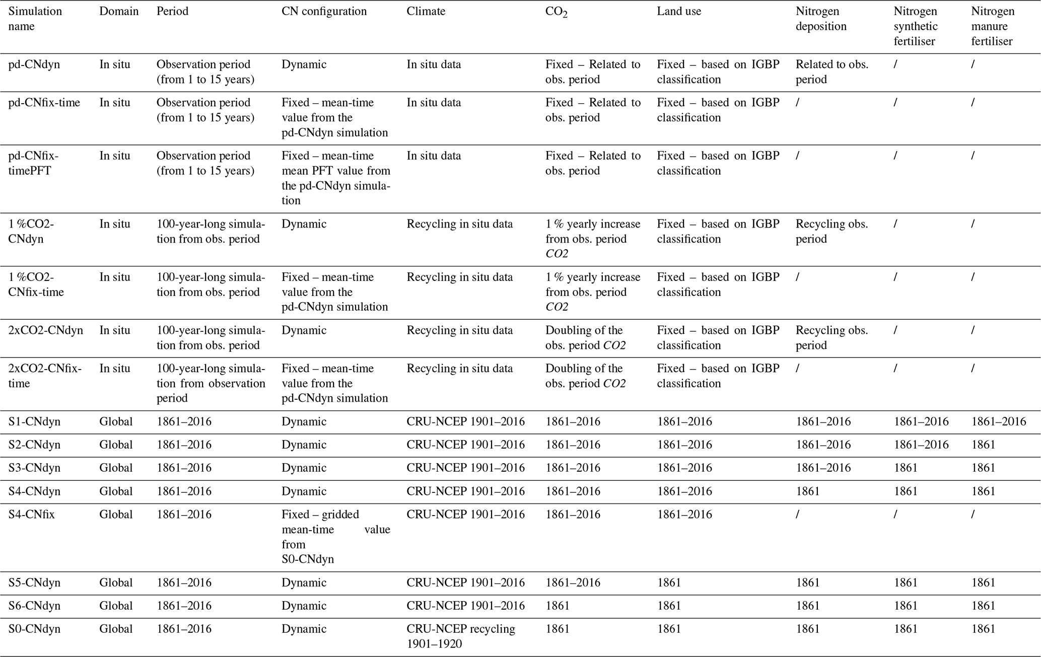
Table 2List of simulations performed in this study and information related to time period, C∕N configuration, and datasets used for climate, CO2, land use, nitrogen deposition, nitrogen synthetic fertiliser and nitrogen manure fertiliser.
Likewise, from the global steady state corresponding to the end of the spin-up simulation, a transient simulation from 1861 to 2016 is run, accounting for climate change, [CO2] rise, land-use change (LUC), and the evolution of nitrogen atmospheric deposition (Ndep), nitrogen synthetic fertiliser (Nfert) and manure (Nman) on a yearly basis. CRU-NCEP data for the period 1901–1920 were used to simulate the period from 1861 to 1901, while from 1901 onwards the climatic forcing from the matching year was used. This simulation, which accounts for carbon–nitrogen interactions, is named S1-CNdyn (Table 2).
2.4.3 Sensitivity test simulations
At each FLUXNET station, different simulations were performed in order to test the sensitivity of ORCHIDEE to different processes or forcing variables. As described in Eq. (5), leaf nitrogen content and leaf C∕N ratio affect the carbon assimilated by photosynthesis, which in turn affects the leaf area index and feeds back to carbon assimilation. Consequently, a set of two simulations was run to investigate the impact of constraining the leaf C∕N ratio on GPP in time and space. One simulation is named pd-CNfix-time (based on the CNfix configuration) in which the leaf C∕N ratio was fixed to the time-average value at site level, which was in turn inferred from the pd-CNdyn reference simulation. In the other simulation named pd-CNfix-timePFT (also based on the CNfix configuration), the leaf C∕N ratio was set to the time-average PFT average, which was also inferred from the pd-CNdyn reference simulations.
The sensitivity of the simulated GPP to [CO2] increase (keeping the other drivers constant) was tested by comparing four idealised 100-year-long simulations against control simulations for which atmospheric [CO2] was held constant at its present-day concentration. A set of simulations started from present-day atmospheric [CO2], and [CO2] was increased by 1 % per year (labelled 1 %CO2). With the present-day [CO2] level around 380 ppm, a 1 % increase per year leads to a near tripling of [CO2] between the start and end of the simulation. In the other set of simulations (labelled 2xCO2), [CO2] was set to twice its present-day value along the 100 years. Both set-ups were repeated for the CNdyn and CNfix-time configurations, thus resulting in a total of four idealised tests (1 %CO2-CNdyn, 1 %CO2-CNfix-time, 2xCO2-CNdyn and 2xCO2-CNfix-time simulations; see Table 2). For these sensitivity tests, climate drivers and nitrogen deposition files corresponding to the period of in situ observations were used cyclically.
At global scale, in addition to the reference S1-CNdyn simulation, sensitivity tests were set up to disentangle the main drivers of the simulated global increase in GPP (see Table 2). Based on the N2O Model Intercomparison Project protocol (Tian et al., 2018), additive scenarios were developed in which GPP is driven by the following using the different forcing data presented in Sect. 2.3: only climate change (S6-CNdyn); climate change and [CO2] increase (S5-CNdyn); climate change, [CO2] increase and land-use change (S4-CNdyn); climate change, [CO2] increase, land-use change and nitrogen deposition evolution (S3-CNdyn); and climate change, [CO2] increase, land-use change, nitrogen deposition and nitrogen fertiliser evolution (S2-CNdyn). A control simulation named S0-CNdyn was also performed, which extends the spin-up simulation (i.e. using the nitrogen input data, the [CO2] value and land use of the year 1860 and recycling the meteorological data of the period 1901–1920).
To test the impact on the GPP evolution of accounting for the carbon–nitrogen interactions, an additional simulation was run at global scale in which the gridded leaf C∕N ratio was fixed to the time-average value for each PFT, inferred from the S0-CNdyn control simulation. Thus, the plant nitrogen status of each PFT within each grid cell is the one of the pre-industrial era (i.e. for the year 1860). In this simulation, all drivers were varied over the period 1861–2016. However, the GPP is insensitive to the variation of nitrogen deposition, nitrogen fertilisation and N from manure in the CNfix configuration, so this simulation corresponds to an S4 scenario and is consequently named S4-CNfix.
2.5 Evaluation metrics
The mean seasonal cycle of the simulated GPP was evaluated against observations. This was done at the PFT level by computing the mean seasonal cycle averaged for all years and all sites belonging to a PFT. Alternatively, simulated daily GPP fluxes were evaluated by computing their root mean squared deviation (root mean square error – RMSE) to the observations. Further, the mean squared deviation (mean square error – MSE) of the daily fluxes to the observation was decomposed and the contribution to the overall MSE from the mean bias, standard deviation and correlation was quantified based on the method of Kobayashi and Salam (2000). MSE can be written as
where SB is the squared bias, SDSD is the squared difference between standard deviations and LCS the lack of correlation weighted by the standard deviations. SB, SDSD and LCS reflect respective errors on bias, standard deviation and correlation. Finally, annual mean GPP flux was computed at each FLUXNET site in order to evaluate the model capacity to simulate site-to-site variations within each PFT.
The global S1-CNdyn simulation was also evaluated by comparing the spatial distribution of the annual mean GPP over the period 2005–2016 to the one of the MTE-GPP product. Furthermore, the time evolutions of the annual GPP, simulated by ORCHIDEE and derived from MTE-GPP, were compared for different regions: globally, Northern Hemisphere (>25∘ N), Southern Hemisphere (<25∘ S) and tropical regions (<25∘ N and >25∘ S).
Lastly, the relative contributions of the different drivers to the present-day GPP value were assessed by computing the successive differences between additive scenarios. Thus, the contributions of climate change, [CO2] increase, land-use change, nitrogen deposition, nitrogen fertilisation and nitrogen manure were respectively provided by the differences between S6 and S0, S5 and S6, S4 and S5, S3 and S4, S2 and S3, and S1 and S2. Using this methodology, the sum of the individual contributions is additive and equals the present-day GPP, thus ignoring possible non-linear interactions between drivers.
3.1 Site-level simulations
3.1.1 Evaluation of the standard configuration
The mean seasonal cycle of the GPP averaged per plant functional type was reproduced for most PFTs in the pd-CNdyn simulations (Fig. 1a). Over tropical evergreen broadleaved forests, the observed mean GPP values do not show a marked seasonal cycle, while the simulated GPP values are 3.0 g C m−2 d−1 higher in May–June compared to the rest of the year. For temperate evergreen needleleaf forests, the mean seasonal cycle simulated by ORCHIDEE matched the observations in terms of correlation (correlation coefficient of 0.99) and amplitude (model standard deviation of 2.4 g C m−2 d−1 to compare to 2.1 for observations), although the simulated GPP was overestimated by ∼30 % all year. The model has the weakest performance for temperate evergreen broadleaved forest shown by a seasonal cycle that is too pronounced compared to that observed (model standard deviation of 2.1 g C m−2 d−1 compared to 0.7 g C m−2 d−1 for observations). In winter and early spring, GPP was overestimated by 2.0 g C m−2 d−1, while later in June and July the decrease in the GPP was overestimated. Simulated and observed mean seasonal cycles match each other for temperate deciduous broadleaved forests, the main discrepancy being a delay of ∼10 d in the onset and senescence phases of the simulated GPP. The simulated mean seasonal cycle of the GPP over boreal evergreen needleleaf forests overestimated GPP by ∼35 % all year, while the variations of the simulated GPP were in agreement with those observed (correlation coefficient of 0.96 and model SD of 2.4 g C m−2 d−1 compared to 1.9 g C m−2 d−1 for observations). Last, over natural C3 grasslands, the increase in GPP at the early stage of the growing season simulated by ORCHIDEE was too slow compared to observations, and the simulated GPP maintained its maximal value too long and too late in the season. This results in a low correlation between the model and observation (correlation coefficient of 0.81).
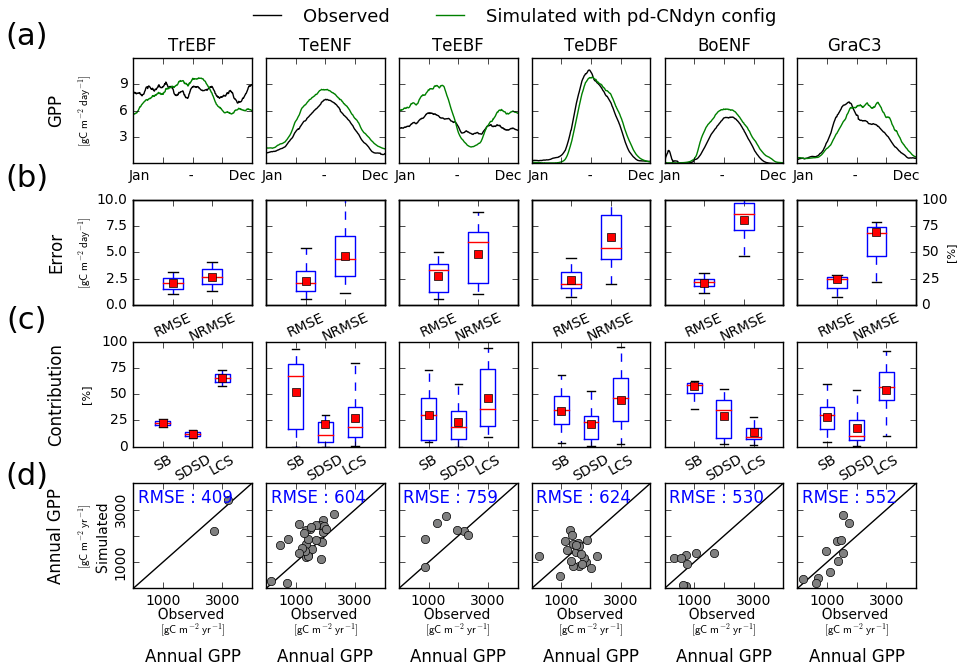
Figure 1Site-level evaluation of ORCHIDEE r4999 simulations against FLUXNET observations. (a) Vegetation class mean seasonal variations of GPP, (b) root mean square error (RMSE) and normalised root mean square error (NRMSE) of simulated daily variations of GPP per vegetation class, (c) attribution of the mean square error (MSE) of the daily variations of GPP to model errors on mean value (SB), standard deviation (SDSD) or correlation (LCS) (Kobayashi and Salam, 2000), and (d) simulated vs. observed annual mean GPP at site level. In panels (b) and (c), the box extends from the lower (25 %) to upper quartile (75 %) values of the data, with a red line at the median and a red square at the arithmetic mean. The whiskers extend from the box to show the range of the data within the 1.5×(25 %–75 %) data range.
The RMSE of the daily GPP flux averaged per PFT does not exceed 2.5 g C m−2 d−1 (Fig. 1b). The annual productivity of the PFTs being significantly different, the RMSE, when expressed as a percentage of the mean annual GPP (NRMSE), varies from 25 % for tropical evergreen broadleaved forests to 80 % for boreal evergreen needleleaf forests. RMSE was plotted against the length of the in situ meteorological data (not shown) to check whether under-sampling of the climate variability explained part of the bias. The data did not support such a relationship (correlation −0.218, 95 % confidence interval (CI) −0.448–0.004). Figure 1c shows the respective contributions of SB (bias), SDSD (deviation) and LCS (correlation) to the total MSE per PFT. These relative contributions to the MSE differed depending on the PFT. Error on the mean bias was the largest contribution to MSE for temperate and boreal evergreen needleleaf forests. At tropical evergreen broadleaved forests and C3 grassland sites, errors on the correlation contributed the most to the MSE, while at temperate evergreen and deciduous broadleaved forest sites, the three sources of error were more equally distributed.
The simulated annual mean GPP per site was comparable to the one observed for most sites (Fig. 1d), with an RMSE averaged per PFT which varied from 409 g C m−2 yr−1 (for tropical evergreen broadleaved forests) to 759 g C m−2 yr−1 (for temperate evergreen broadleaved forests). Both overestimation and underestimation were observed in all PFTs, suggesting small systematic biases. Site-to-site variations of the annual mean GPP were relatively well reproduced for tropical evergreen broadleaved forests, temperate evergreen needleleaf forests, temperate evergreen broadleaved forests and C3 grassland sites (with respective Pearson's correlation coefficients of 1.0 – but for only two sites – 0.63, 0.44 and 0.82) but not for temperate deciduous broadleaved forest and boreal evergreen needleleaf forest sites (Fig. 1d). For temperate deciduous broadleaved forest sites, the model produces significantly larger site-to-site GPP differences than the observations.
In order to analyse how ORCHIDEE r4999 performs compared to r3977 (reference version without the nitrogen cycle), we evaluated the GPP simulated by ORCHIDEE r3977 against FLUXNET observations (Fig. B1). The model–data agreement for r3977 was comparable to the one for r4999 but slightly better. In particular, the NRMSE of the simulated daily GPP flux (Fig. B1b) and the RMSE of the simulated annual mean GPP (Fig. B1d) were lower in r3977 compared to r4999 for temperate evergreen needleleaf and broadleaved forests as well as temperate deciduous broadleaved forest sites. Particularly for temperate evergreen needleleaf and broadleaved forests sites, the lower mean NRMSE of the simulated daily GPP at the PFT level for r3977 was due to a narrower range of NRMSE values at site level (whisker boxes are narrower), indicating that the NRMSE was not systematically lower at all sites but only at some specific ones.
Because the GPP flux is intimately linked to the transpiration flux through stomatal control, a site-level evaluation of the pd-CNdyn simulation has been performed against site-level observations of the latent heat (LE) flux (Fig. C1), an energy flux to which transpiration contributes, as does soil evaporation. Overall, the model performed better at simulating LE variations than variations in GPP. This was particularly true when looking at the NRMSE of the simulated daily flux, which never exceeded 50 % as a mean average score at the PFT level for LE, while it reached values up to 75 % for GPP for some PFTs (BoENF and GraC3).
3.1.2 Sensitivity to model configurations
The leaf C∕N ratio in the pd-CNdyn simulation varied substantially over time and/or from one site to another (Fig. 2c). The observed variation was partly driven by the different nitrogen deposition load (Fig. 2a and b) as well as by differences in the simulated mineralisation and plant nitrogen uptake (not shown). Vcmax being directly related to the leaf nitrogen content, the variations of the leaf C∕N ratio induced seasonal variations of the Vcmax on the order of 0 % to 30 %, depending on the sites.
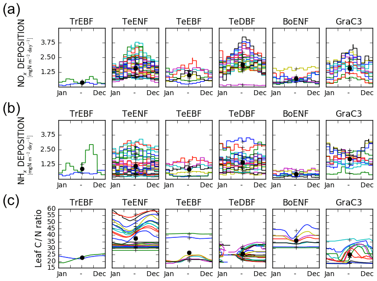
Figure 2Mean seasonal variations of factors driving the simulated GPP at each site per PFT class. (a) Variation of the deposition of NOx compounds, (b) variation of the deposition of NHx compounds and (c) variation of the leaf C∕N ratio. Each site is represented by a different colour. The black crosses denote the time-averaged value for each site and the black dots show the time-averaged and site-averaged value for each PFT. Missing data for the leaf C∕N ratio of temperate deciduous broadleaved forests are due to the absence of leaves.
The mean and median values of the MSE of the simulated daily GPP obtained from the range of sites within a vegetation class did not change substantially depending on whether nitrogen dynamics were accounted for or were fixed over time (pd-CNdyn, pd-CNfix-time or pd-CNfix-timePFT) (Fig. 3a). This finding holds for the error measures when decomposed into bias, standard deviation and correlation (Figs. 3b–d). One exception to this model behaviour, which is common across configurations, is that there were some C3 grassland sites where MSE and all its components were higher in the pd-CNfix-time and pd-CNfix-timePFT simulations compared to the pd-CNdyn simulation (Fig. 3). For tropical and temperate evergreen broadleaved forest classes, the CNfix-time simulation exhibits narrower ranges for MSE or for some of its components (SB, SDSD or LCS) compared to the pd-CNdyn simulation. This highlights the fact that, for some of the tropical and temperate evergreen broadleaved forest sites, constraining the leaf C∕N ratio in time improved the fit to the observed GPP, while the same constraint deteriorated the fit at some other sites within that PFT. Results obtained with the pd-CNfix-timePFT simulation also lead to slightly narrower ranges of MSE values and its bias (SB) subcomponent for temperate evergreen needleleaf forest compared to the pd-CNfix-time simulation.
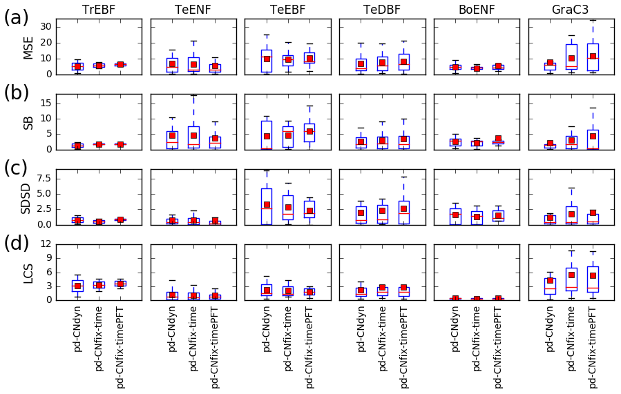
Figure 3Sensitivity of the model performance to the model configuration. Distribution at the plant functional type level of the mean square error (MSE) of the daily GPP variations at each site and contribution to the MSE of model errors on mean value (SB), standard deviation (SDSD) or correlation (LCS) for the pd-CNdyn, pd-CNfix-time and pd-CNfix-timePFT simulations. The box extends from the lower (25 %) to upper quartile (75 %) values of the data, with a red line at the median and a red square at the arithmetic mean. The whiskers extend from the box to show the range of the data within the 1.5×(25 %–75 %) data range.
Simulated site-to-site variations of the annual mean GPP were sensitive to the model configuration regarding the leaf C∕N ratio (Fig. 4). For all PFTs except the boreal evergreen needleleaf forest sites, the pd-CNdyn is the simulation which best matched the observations in terms of RMSE. Nevertheless, the RMSEs were of the same order of magnitude for the three model configurations for all PFTs except for C3 grassland sites, for which the RMSE was significantly lower in the pd-CNdyn simulation (Fig. 4).
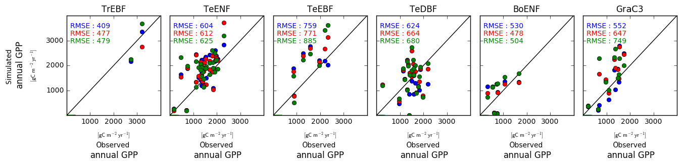
Figure 4Simulated vs. observed annual mean GPP at site level. Blue dots are for a model configuration in which the leaf C∕N ratio varies between sites and across time (pd-CNdyn); the red dots represent a configuration in which the leaf C∕N ratio varies across sites but was fixed across time (pd-CNfix-time), and the green dots represent a configuration in which the leaf C∕N ratio was fixed across sites and time (pd-CNfix-timePFT).
3.1.3 Sensitivity to [CO2] increase
Increasing atmospheric [CO2] by 1 % per year leads to a continuous increase in the GPP in any of the two configurations: one with dynamic leaf C∕N ratios (1 %CO2-CNdyn) and the other with leaf CN ratios fixed over time (1 %CO2-CNfix-time) for any PFT class (Fig. 5). Note first that the large temporal cycle for the tropical evergreen broadleaved forest is due to the recycling of 2 to 4 years of in situ meteorological forcing. As expected, the higher the [CO2], the higher the GPP. Nevertheless, the GPP increase was less sensitive to the [CO2] increase in the configuration with a dynamic C∕N ratio (1 %CO2-CNdyn), which reflects an induced nitrogen limitation of the photosynthesis. Notably, the GPP sensitivity to CO2 increase in the 1 %CO2-CNdyn simulation was particularly low for the boreal evergreen needleleaf forest class. After 100 years of [CO2] increase, the difference in GPP increase between the 1 %CO2-CNfix-time and 1 %CO2-CNdyn simulations reached 1.0 kg C m−2 yr−1 for tropical evergreen broadleaved forests, 0.8 kg C m−2 yr−1 for temperate evergreen needleleaf forest, 0.8 kg C m−2 yr−1 for temperate evergreen broadleaved forest, 0.6 kg C m−2 yr−1 for temperate deciduous broadleaved forest, 0.6 kg C m−2 yr−1 for boreal evergreen needleleaf forest and 1.0 kg C m−2 yr−1 for C3 natural grasslands. These differences in GPP increase corresponded to values of the order of 30 %–50 % of the present-day annual mean GPP.
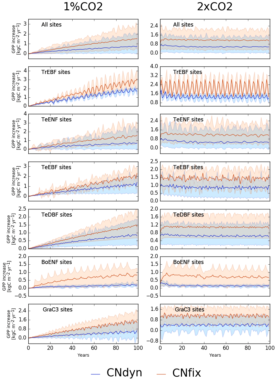
Figure 5Effect of changes in the atmospheric CO2 concentration on GPP. Annual mean GPP difference (kg C m−2 yr−1; mean; 5th and 95th percentile) between the EXP-CNdyn and pd-CNdyn simulations (in blue) and the EXP-CNfix-time and pd-CNfix-time simulations (in red) for the different PFTs; EXP stands for 1 %CO2 (left column) and 2xCO2 (right column). A relative time axis was used because the simulations started the year following the last observational year in the FLUXNET database, which may differ across sites.
In the simulation in which [CO2] was doubled compared to the present-day level but N limitation was not accounted for (2xCO2-CNfix-time), GPP increased by 90 % overall (1.1 kg C m−2 yr−1; Fig. 5) and at some sites even by as much as 150 %. Accounting for N limitation (2xCO2-CNdyn simulation) reduced the overall GPP increase to ∼50 % compared to the present-day value (0.6 kg C m−2 yr−1; Fig. 5). A decreasing trend in GPP increase for all PFTs – except temperate deciduous broadleaved forest and C3 grassland sites – was apparent for the 2xCO2-CNdyn simulation, while such a trend was absent in the simulations without carbon–nitrogen interactions (2xCO2-CNfix-time). For instance, mean GPP increase at temperate evergreen needleleaf forest sites reached 0.8 kg C m−2 yr−1 over the 5 years consecutive with the doubling of the CO2 level but was only 0.5 kg C m−2 yr−1 after 100 years (Fig. 5). Furthermore, when comparing the simulations without and with N limitations, the year-to-year variability in GPP was amplified compared to the present-day variability for the configuration without N limitation.
GPP increase induced by an increase in atmospheric [CO2] was achieved at a limited water cost or even resulted in saving water at most sites. In the 1 %CO2-CNfix-time simulations, after 100 years of [CO2] increase, the transpiration rate averaged per PFT was lower by a few millimetres (up to 50 mm per year) compared to its value in the pd-CNfix-time simulation (Fig. 6, left column). Averaged over all PFTs, the mean transpiration rate decreased by ∼25 mm yr−1 after 100 years. In the 1 %CO2-CNdyn simulation, the decrease in the transpiration rate was even stronger (Fig. 6). Mean transpiration rate decrease averaged per PFT reached 75 to 110 mm per year after 100 years. Averaged over all sites, the mean decrease equalled 100 mm per year, which corresponds to ∼20 % of its value in the pd-CNdyn simulation. Similar model behaviour with the 2xCO2-type simulations was exhibited (Fig. 6, right column). Compared to its value in the pd-CNfix-time simulation, the mean transpiration rate averaged over all sites was stable in the 2xCO2-CNfix-time simulation. In the 2xCO2-CNdyn simulation, the mean transpiration rate was 50 mm per year lower than it was in the pd-CNdyn simulation (15 %).
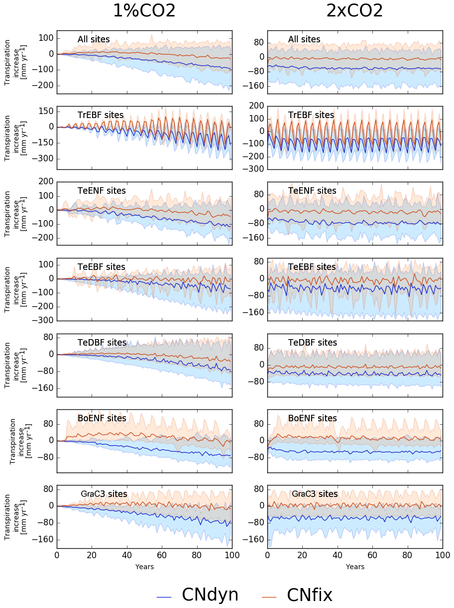
Figure 6Effect of changes in the atmospheric CO2 concentration on transpiration. Annual mean transpiration difference (kg[H2O] m−2 yr−1; mean; 5th and 95th percentile) between the EXP-CNdyn and pd-CNdyn simulations (in blue) and the EXP-CNfix-time and pd-CNfix-time simulations (in red) for the different plant functional types; EXP stands for 1 %CO2 (left column) and 2xCO2 (right column). A relative time axis was used because the simulations started the year following the last observational year in the FLUXNET database, which may differ across sites.
When expressed in terms of water-use efficiency (WUE; unitless) – defined here as the ratio of GPP (g C m−2 yr−1) to transpiration (g H2O m−2 yr−1) – these model responses translated into an increase in the WUE for all the sensitivity tests (Fig. 7). Under the 1 %CO2-CNfix-time simulation, after 100 years, WUE increased by 120 % on average per PFT (Fig. 7; mean increase of 120 %) compared to the pd-CNfix-time simulation. After 100 years, the mean WUE increase in the 1 %CO2-CNdyn simulation is 17 % lower than in the 1 %CO2-CNfix-time simulation. Similarly, the mean WUE averaged per PFT in the 2xCO2-CNfix-time simulation is 70 % to 90 % higher than in the pd-CNfix-time simulation (mean increase of 80 % over all sites; Fig. 7). In the 2xCO2-CNdyn simulation, the mean increase in the WUE is 10 % lower than in the 2xCO2-CNfix-time simulation.
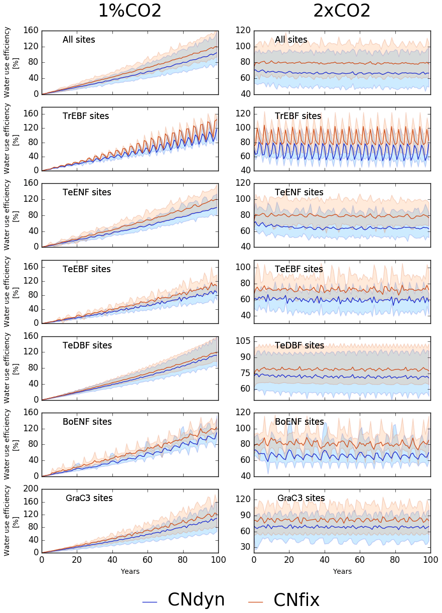
Figure 7Effect of changes in the atmospheric CO2 concentration on water-use efficiency (WUE). Annual mean WUE relative difference (percentage; mean; 5th and 95th percentile) between the EXP-CNdyn and pd-CNdyn simulations (in blue) and the EXP-CNfix-time and pd-CNfix-time simulations (in red) for the different plant functional types; EXP stands for 1 %CO2 (left column) and 2xCO2 (right column). A relative time axis was used because the simulations started the year following the last observational year in the FLUXNET database, which may differ across sites.
3.2 Global-scale simulations
The present-day annual mean GPP under the S1-CNdyn simulation reached its maximum values in central Africa (Fig. 8a). Compared to values reported by MTE-GPP (Jung et al., 2011), simulated annual mean GPP in this region is overestimated by up to 2.0 kg C m−2 yr−1 (Fig. 8b). On the other hand, annual mean GPP values in the Amazon region and Indonesia were underestimated by 1.5 kg C m−2 yr−1. Overall, the root mean square deviation of the MTE-GPP values equals 0.7 kg C m−2 yr−1 compared to the global mean annual flux from MTE-GPP of 1.0 kg C m−2 yr−1. With the difference between the simulations and MTE-GPP data being less than 0.5 kg C m−2 yr−1 in most extratropical regions, the root mean square deviation is thus dominated by the mismatch between the simulations and observations over the tropics.
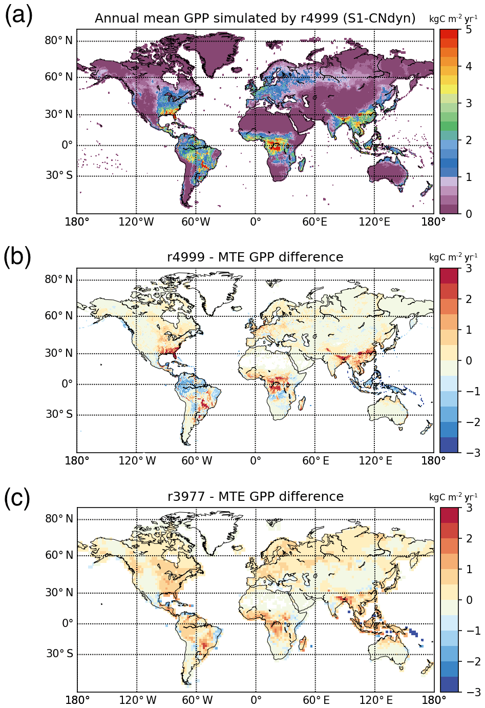
Figure 8Global-scale evaluation of ORCHIDEE against the observation-based MTE-GPP product. (a) Global distribution of the simulated annual mean GPP by ORCHIDEE r4999 (kg C m−2 yr−1) over 2001–2010; (b) global distribution of the difference between the simulated annual mean GPP by ORCHIDEE r4999 and the MTE-GPP product; (c) global distribution of the difference between the simulated annual mean GPP by ORCHIDEE r3977 and the MTE-GPP product.
When summed by latitudinal band, the overlap between simulated annual mean GPP and MTE-GPP estimates increases (Fig. 9) compared to the overall global mapping result. From 1982 to 2008, the simulated annual mean GPP above 25∘ N increased from 36 to 42 Pg C yr−1 (approximate 17 % increase), with large year-to-year variations (up to 3 Pg C yr−1) (Fig. 9a). Over the same period and the same domain, the MTE-GPP estimates varied between 37 and 40 Pg C yr−1 (approximate 8 % increase), thus showing a weaker positive trend compared to the ORCHIDEE simulation. In the tropical regions (between 25∘ S and 25∘ N), the MTE-GPP estimate varied from 72 to 75 Pg C yr−1 (approximate 4 % increase) between 1982 and 2008, while according to the ORCHIDEE S1-CNdyn simulation, GPP strongly increased from 62 to 72 Pg C yr−1 (approximate 16 % increase) over the same period (Fig. 9b).
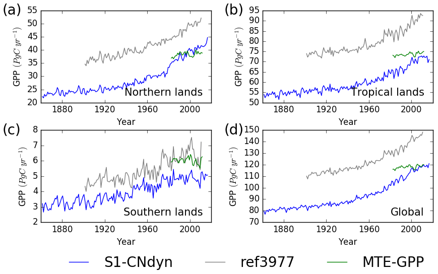
Figure 9Evaluation of GPP from ORCHIDEE against the observation-based MTE-GPP product for four regions. Time evolution of the annual mean GPP (Pg C yr−1) estimated by ORCHIDEE r4999 (in blue), ORCHIDEE r3977 (in grey) and the observation-based MTE-GPP product (in green) for (a) northern lands (>25∘ N), (b) tropical lands (<25∘ N and >25∘ S), (c) southern lands (<25∘ S) and (d) all lands.
Due to a lower land area and a lower productivity per unit of land, the contribution of the southern lands (below 25∘ S) to the global GPP is rather small. It amounts 5 Pg C yr−1 with ORCHIDEE and 6 Pg C yr−1 with MTE-GPP over the 1982–2008 period (Fig. 9c). Both estimates have no trend over the time period and the year-to-year variations are slightly larger with the ORCHIDEE model (standard deviation of 0.3 Pg C yr−1 compared to 0.2 Pg C yr−1 with MTE-GPP). Globally, annual mean GPP reached ∼120 Pg C yr−1 in 2016 (Fig. 9d).
Similarities between the simulated global distributions and biases in GPP and LAI (compare Fig. D1a to Fig. 8a and Fig. D1b to Fig. 8b) suggest that a GPP bias reduction may potentially be obtained from LAI modelling improvements. The model–data agreement for LAI when averaged per latitudinal band (Fig. E1) is comparable to the one for GPP (Fig. 9), with a good agreement for the northern and tropical lands and model underestimation in the southern lands.
The agreement between the modelled and observed annual mean LAI and GPP summed over three latitudinal bands, as well as at the global scale, was higher for r4999 (i.e. S1-CNdyn simulation) compared to r3977 without the nitrogen cycle (see Figs. 9 and E1); r3977 systematically overestimated LAI and GPP for any region, except for the southern lands where r3977 provided similar values as the GIMMS and MTE-GPP products. Compared to the GIMMS and MTE-GPP products, gridded annual mean LAI and GPP values simulated by r3977 were overestimated in the northern lands, with biases exceeding those found in r4999. In contrast, biases of r4999 were higher than those of r3977 in the tropical regions, in particular in central Africa (see Figs. 8 and D1).
Over the period 1861–2016, when accounting for all driving variables (S1-CNdyn simulation), simulated global GPP increased by ∼50 % from 80 to 120 Pg C yr−1 (Fig. 10a; 39 % over the 20th century). When only driven by climate change and [CO2] increase (S5-CNdyn simulation), simulated GPP varied from 80 Pg C yr−1 in 1861 to 104 Pg C yr−1 in 2016 (∼30 % increase). Similarly, without the increase in nitrogen fertilisation (S3-CNdyn simulation), global GPP would only have increased by 34 % over the same period. The relative contributions of the different drivers to the GPP growth over 1861–2016 were 10 % for climate change, 50 % for [CO2] increase, −13 % for land-use change, 20 % for nitrogen deposition change and 33 % for nitrogen fertilisation change. Global GPP evolution under the S4-CNfix simulation is similar to that under the S1-CNdyn simulation (Fig. 10a). These simulated GPP responses to variations of driving factors are not equally distributed across PFTs. Thus, simulated GPPs over all forested lands (Fig. 10b) and over all grasslands and croplands (Fig. 10c) show contrasting responses. In particular, simulated present-day GPP over forested lands equals ∼63 Pg C yr−1 under the S1-CNdyn simulation (Fig. 10b) and ∼82 Pg C yr−1 under the S4-CNfix simulation. In contrast, GPP over grasslands and croplands (Fig. 10c) equals 56 Pg C yr−1 under the S1-CNdyn simulation but only 43 Pg C yr−1 under the S4-CNfix simulation.
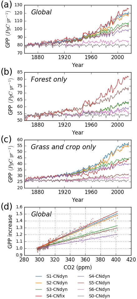
Figure 10Impact of key driving factors on the global annual mean GPP simulated by ORCHIDEE. (a) Simulated global annual mean GPP (Pg C yr−1) as a function of time from 1860 to 2016; (b) simulated annual mean GPP (Pg C yr−1) of all forest lands from 1860 to 2016; (c) simulated annual mean GPP (Pg C yr−1) of all grasslands and croplands from 1860 to 2016; (d) simulated global annual mean GPP (relatively to its 1900 value) as a function of the [CO2] level. S0-CNdyn to S6-CNdyn are seven additive scenarios in which driving factors are added one at a time, and S4-CNfix is a scenario in which the leaf C∕N ratios of each PFT within each grid cell are fixed to their mean-time pre-industrial values (see Sect. 2.4.3 and Table 2 for details). In panel (b), blue, orange and green lines (for the S1-CNdyn, S2-CNdyn and S3-CNdyn scenarios, respectively) overlap because synthetic fertiliser and manure applications are not considered on forested lands and consequently have no impact on GPP.
We presented revision 4999 of the ORCHIDEE model that accounts for carbon–nitrogen interactions based on the initial work of Zaehle and Friend (2010). In this model version, improvements were implemented with respect to the water, energy and carbon budgets, as well as the nitrogen cycle and its coupling to the carbon cycle, compared to the original version of ORCHIDEE used in Zaehle and Friend (2010). Among these changes, a new carbon assimilation scheme was introduced (Yin and Struik, 2009) in which the maximum Rubisco-activity-limited carboxylation rate is a direct function of the leaf nitrogen content (Kattge et al., 2009). Because these model developments primarily impact the GPP and because this flux is the primary carbon input flow into the ecosystem, we focussed our study on an in-depth evaluation of the simulated GPP flux from the site to global scale and from a daily to mean annual timescale.
We showed that the version of ORCHIDEE (r4999) that accounts for carbon–nitrogen interactions can simulate reasonably well the mean seasonal cycle, daily mean variations and annual mean GPP for most PFTs. The overlap between the ORCHIDEE simulations and the eddy-covariance-based observations is similar to other models (Balzarolo et al., 2014; Slevin et al., 2015). For instance, based on an evaluation over 32 FLUXNET sites, Balzarolo et al. (2014) reported mean RMSE values of the daily GPP flux simulated by three GTEMs (i.e. ORCHIDEE, CTESSEL and ISBA-A-gs) which range between 1.9 and 4.4 g C m−2 d−1 depending on the model and PFT considered (excluding cropland sites for which all models performed the least well and which are not included in our study). In comparison, the mean RMSE of the simulated daily GPP flux in our study for any PFT never exceeded 2.5 g C m−2 d−1.
The exception to the general agreement is for the temperate evergreen broadleaved forest sites, for which ORCHIDEE r4999 failed to reproduce the observed mean seasonal cycle. Indeed, the weak performances are for the five Mediterranean sites but not for the two Australian sites. The Mediterranean sites receive high N-deposition loads, leading to low leaf C∕N ratios. Over these sites, at the beginning of the growing season, the higher maximum Rubisco-activity-limited carboxylation rate values (Vcmax) induced by high leaf nitrogen content is the main reason explaining the GPP overestimation. The overestimation of the GPP at the early stage of the growing season induced higher rates of transpiration. These higher rates of transpiration partly explain the underestimation of the GPP during the summer due to a depletion of the soil water that is too strong. Because the GPP is too low during the summer and demands less nitrogen to support biomass growth, this results in higher nitrogen availability later in the season. This mechanism tends to maintain or even amplify the mismatch at the beginning of the growing season. The two Australian sites receive low N-deposition loads in comparison to the three Mediterranean sites. Consequently, the Australian sites have high leaf C∕N ratios (see Fig. 2c for TeEBF; Australian sites correspond to the blue and green lines), which overcomes the overestimate of the GPP at the beginning of the growing season and the subsequent issues.
Global-scale annual mean GPP simulated by ORCHIDEE and aggregated per latitudinal band matches GPP estimated by the MTE-GPP product. The temporal increase in GPP projected by ORCHIDEE for the northern and tropical regions is not apparent from the MTE-GPP. Indeed, the MTE-GPP is only driven by the climate variability, vegetation greenness index and land cover information. As such, MTE-GPP does not directly represent the effect of CO2 and nitrogen on the GPP but only indirectly through changes in vegetation greenness. This conceptual limitation may explain the absence of trends in the GPP signal from MTE-GPP and restricts the domain of validity of this product to the period over which it has been trained. The aforementioned limitation may also explain part of the spatial disagreement between ORCHIDEE and MTE-GPP. Nevertheless, GPP appears significantly biased – against MTE-GPP – over the tropical regions, with positive biases in central Africa and negative ones in Amazonia. One may note that these biases do not show such contrast in the original ORCHIDEE version without the nitrogen cycle (r3977; see Fig. 8c). Further analyses showed that the GPP biases over tropical forest regions are driven by different leaf C∕N ratios across regions. However, it remains unclear what are the primary drivers of the spatial variation of the leaf C∕N ratio and consequently of GPP. One of the drivers is likely to be NOx deposition, which is lower in Amazonia compared to central Africa (not shown). There is no such relationship between GPP and BNF rate, nor between GPP and NHx deposition rate, in tropical regions. The drivers and/or processes that are responsible for turning large-scale differences in NOx deposition into fine-scale differences in GPP have yet to be identified.
Apart from the MTE-GPP product, there are few spatially explicit data available that are suitable to evaluate global simulations of GPP. Due to the fact that two CO2 fluxes occur at land but have an opposite direction (i.e. GPP and total ecosystem respiration), data of atmospheric [CO2] cannot be used for this purpose. As an alternative, Campbell et al. (2017) assessed the GPP growth rate over the 20th century based on an independent estimate by using atmospheric carbonyl sulfide (COS) records. Based on a procedure that optimises the COS sources and sinks to match the observed atmospheric [COS] dynamic, they deduce that the GPP increased by 31 % ± 5 % over the 20th century. This corresponds to a larger GPP growth rate than that estimated by most global terrestrial ecosystem models. Although higher than the 31 % ± 5 % based on the COS constraint, the ORCHIDEE-based 39 % is in good agreement with the COS constraint compared to most other ecosystem models reported in the study of Campbell et al. (2017). This increases our confidence in the ability of ORCHIDEE r4999 to account for the interactions between carbon and nitrogen.
Constraining the leaf C∕N ratio over time and per PFT (using the values from a simulation with dynamic C∕N ratios) was found not to impact model performance at site level for most PFTs. Note, however, that the leaf C∕N ratios in the pd-CNfix-time and pd-CNfix-timePFT simulations were set using the present-day values from the pd-CNdyn simulation. At some sites, the mean standard error of the simulated daily mean GPP variation is reduced, but an increase in mean standard error was observed at other sites. At first, the similarity in performance for configurations with and without a dynamic leaf C∕N ratio may appear as a failure in terms of expected impacts with the inclusion of the nitrogen cycle in the model. Accounting for a dynamic leaf C∕N ratio and for site-specific information such as nitrogen deposition could be expected, at least from a theoretical point of view, to enhance the predictive power of ORCHIDEE. However, at the same time, dynamic modelling of the leaf C∕N ratio adds complexity and interactions which come with additional sources of uncertainties. Our results indicate that for some sites the increase in predictive power dominates, whereas for other sites the additional uncertainties dominate the total model error.
One exception was the C3 grassland sites for which the mean model performance was lower when carbon–nitrogen interactions were not accounted for (pd-CNfix-time and pd-CNfix-timePFT simulations), leading to a higher mean MSE for this PFT compared to the pd-CNdyn simulation. Constraining (or not) the leaf C∕N ratio (pd-CNfix-time vs. pd-CNdyn configuration) alters GPP via changes to the Vcmax value. Moreover, for some “extreme” conditions in the CNdyn configuration, carbon allocation to the different reservoirs may be reduced due to insufficient nitrogen in the labile pool, irrespective of the value of the C∕N ratio of the standing leaf biomass (see the end of Sect. 2.1.3 where this model behaviour is detailed). These extreme conditions in terms of nitrogen availability and their consequences for biomass allocation cannot be captured with the CN-fix configuration, and it appears that at many C3 grassland sites these extreme conditions are sufficiently frequent to produce different model responses and performances between the pd-CNfix-time and pd-CNfix-timePFT simulations and the pd-CNdyn simulation. A first analysis indicates that the low nitrogen availability is due to a reduction of the nitrogen uptake, which is primary explained by the low fine root biomass rather than a temperature or soil moisture effect on the N uptake.
While behaviour and performance are similar across ORCHIDEE configurations for present-day conditions for most PFTs, they differ substantially in terms of the response of GPP to enhanced atmospheric [CO2]. The site-mean increase in GPP after 100 years under the 1 %CO2 experiment is half when carbon–nitrogen interactions are accounted for compared to ignoring the carbon–nitrogen interactions (CNdyn compared to CNfix-time). Interestingly, this effect size is of the same order of magnitude as the simulated reduction in the increase in net primary production (NPP) (65 %) under Representative Concentration Pathway 8.5 (Wieder et al., 2015) estimated by coupled carbon–climate model projections and C∕N stoichiometric models. The reduction in the increase in NPP was caused by the interaction between enhanced atmospheric [CO2] and nitrogen limitations trends (Wieder et al., 2015).
Simulated site-average GPP increased by 50 % when [CO2] was doubled (370 ppm, 2xCO2 experiment) and carbon–nitrogen interactions were accounted for. A similar response has been reported for some experimental Free-Air Carbon dioxide Enrichment (FACE) sites (Norby et al., 2010; Zaehle et al., 2014) at which GPP increased by 30 % for an increase between 150 and 200 ppm in atmospheric [CO2]. Also, the simulated decrease in the growth rate in GPP over time at some sites is in line with the progressive nitrogen limitation as postulated by Luo et al. (2004). At global scale, we showed that the present-day simulated GPP is reduced by 20 % when the additional nitrogen limitation associated with the period 1860–2016 is accounted for (S4-CNdyn) compared to ignoring this nitrogen limitation (S4-CNfix). We showed that the simulated GPP trajectories from 1861 to 2016 under S1-CNdyn and S4-CNfix (in which the leaf C∕N ratios are fixed to their mean-time pre-industrial values) are similar, meaning that the global historical increase in nitrogen inputs (through deposition and fertilisation) was of the same order as the nitrogen demand to fulfil the GPP increase due to the [CO2] fertilisation effect. This general behaviour, however, hides contrasting responses between classes of PFTs. Over forested lands, the potential GPP increase primarily driven by the [CO2] fertilisation effect has been significantly limited due to a shortage of plant-available nitrogen (compare S4-CNfix and S3-CNdyn curves in Fig. 10b). In contrast, over grasslands and croplands, the supply of nitrogen through fertilisation has fostered the GPP more than it would have done solely from the [CO2] fertilisation effect without N limitation (compare S4-CNfix and S1-CNdyn curves in Fig. 10c).
We showed that accounting for carbon–nitrogen interactions (or not) when atmospheric [CO2] is enriched not only impacts the GPP response but also has important consequences for the transpiration rate. We showed that on average, when atmospheric [CO2] is doubled (∼700–750 ppm), the water-use efficiency – calculated as the ratio between GPP and transpiration – increases by 80 % under the CNfix-time configuration but only by 67 % under the CNdyn configuration. The difference in water-use efficiency change is likely partly the outcome of the nitrogen cycle through its impact on Vcmax and thus on stomatal conductance. Although based on a slightly different indicator, this is well in agreement with the observed increase (+68 %) in the instantaneous transpiration efficiency (computed as the assimilation divided by the stomatal conductance; ITE) reported in the meta-analysis of Ainsworth and Long (2005) based on a set of C3 ecosystem sites where atmospheric [CO2] was enriched to reach atmospheric concentrations between 475 and 600 ppm. Our model experiments illustrate the interplay between the carbon, nitrogen and water cycles and highlight the need for careful analysis when modelling ecosystem productivity under future climate changes and its possible reduction due to water limitation (Ahlström et al., 2012).
We conclude that if carbon–nitrogen interactions are accounted for, the functional responses of ORCHIDEE r4999 better agree with the current understanding of photosynthesis than when the carbon–nitrogen interactions are not accounted for. From this point of view our factorial experiment and sensitivity analysis confirm what has been shown by several other global terrestrial models: i.e. that carbon–nitrogen interactions are essential in understanding global terrestrial ecosystem productivity (Goll et al., 2017; Sokolov et al., 2008; Thornton et al., 2009; Wang and Houlton, 2009; Wania et al., 2012; Wieder et al., 2015; Zaehle et al., 2010a, b), especially its dynamic under atmospheric [CO2] increase and climate change. Further simulations, making use of this new ORCHIDEE version and driven by different socio-economic scenarios over the 21st century (i.e. Representative Concentration Pathways), will be performed in order to better quantify the future GPP response to the combined evolution of [CO2] and nitrogen land supply. Additionally, climate simulations with the IPSL Earth system model (as part of the CMIP6 intercomparison project) including this new ORCHIDEE version are planned to assess the impact of nitrogen limitation on the fate of the net land carbon sink and on climate projections.
The source code is freely available online via the following address: https://doi.org/10.14768/20190724001.1 (Vuichard, 2018).
Table A1List of FLUXNET La Thuile sites used in this study and associated information related to the country, location and corresponding plant functional type in the ORCHIDEE model.
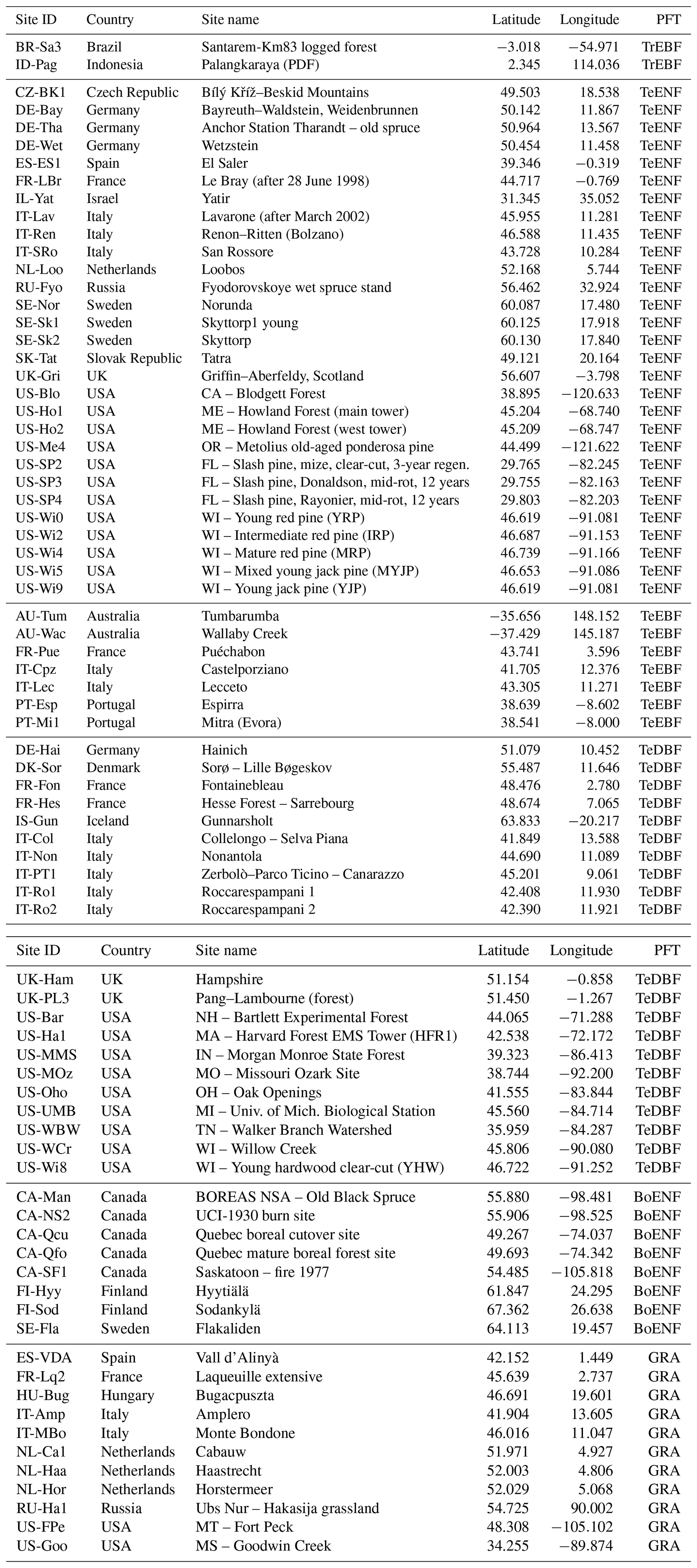
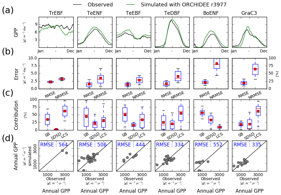
Figure B1Site-level evaluation of ORCHIDEE r3977 (i.e. without N cycle) simulations against FLUXNET observations. (a) Vegetation class mean seasonal variations of GPP, (b) root mean square error (RMSE) and normalised root mean square error (NRMSE) of simulated daily variations of GPP per vegetation class. (c) Attribution of the mean square error (MSE) of the daily variations of GPP to model errors on mean value (SB), standard deviation (SDSD) or correlation (LCS) (Kobayashi and Salam, 2000), and (d) simulated vs. observed annual mean GPP at site level. In panels (b) and (c), the box extends from the lower (25 %) to upper quartile (75 %) values of the data, with a red line at the median and a red square at the arithmetic mean. The whiskers extend from the box to show the range of the data within the 1.5×(25 %–75 %) data range.
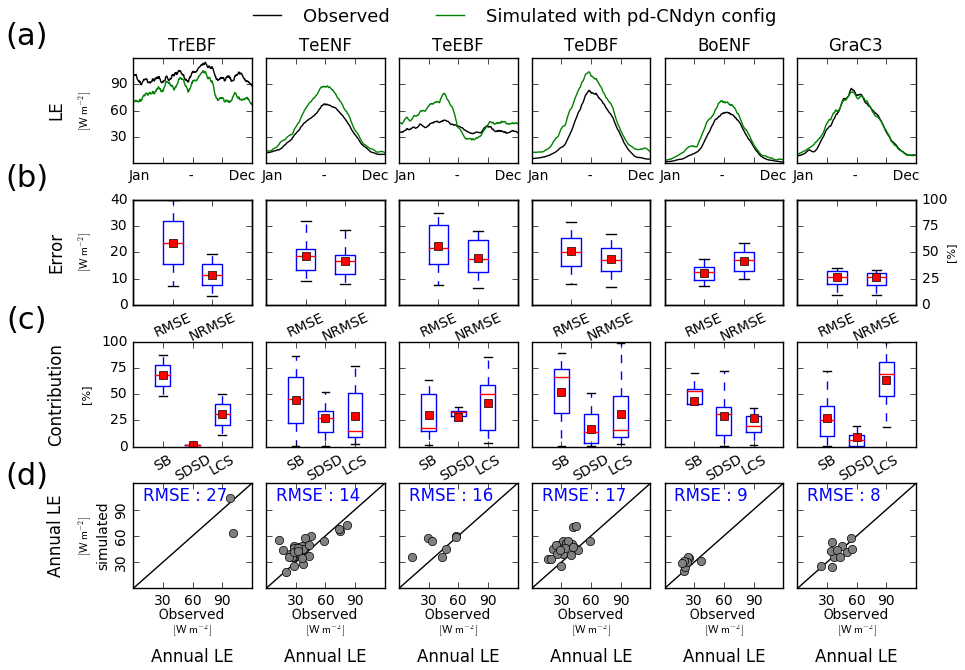
Figure C1Site-level evaluation of ORCHIDEE r4999 simulations against FLUXNET observations. (a) Vegetation class mean seasonal variations of latent heat flux (LE; W m−2), (b) root mean square error (RMSE; W m−2) and normalised root mean square error (NRMSE; %) of simulated daily variations of LE per vegetation class. (c) Attribution of the mean square error (MSE) of the daily variations of LE to model errors on mean value (SB; %), standard deviation (SDSD; %) or correlation (LCS; %) (Kobayashi and Salam, 2000), and (d) simulated vs. observed annual mean LE at site level (W m−2). In panels (b) and (c), the box extends from the lower (25 %) to upper quartile (75 %) values of the data, with a red line at the median and a red square at the arithmetic mean. The whiskers extend from the box to show the range of the data within the 1.5×(25 %–75 %) data range.
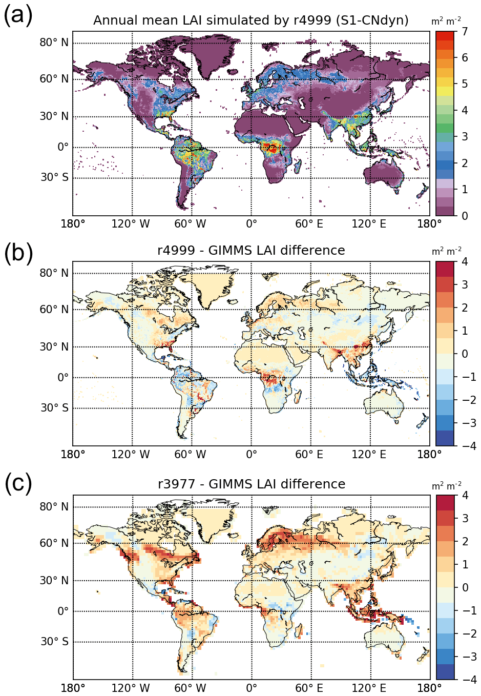
Figure D1Global-scale evaluation of ORCHIDEE against the observation-based GIMMS product. (a) Global distribution of the simulated annual mean LAI by ORCHIDEE r4999 (m2 m−2) over 2001–2010; (b) global distribution of the difference between the simulated annual mean LAI by ORCHIDEE r4999 and the GIMMS product; (c) global distribution of the difference between the simulated annual mean LAI by ORCHIDEE r3977 and the GIMMS product.
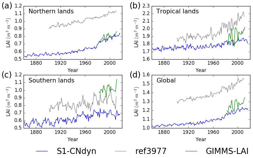
Figure E1Evaluation of LAI from ORCHIDEE against the observation-based GIMMS product for four regions. Time evolution of the annual mean LAI (m2 m−2) estimated by ORCHIDEE r4999 (in blue), ORCHIDEE r3977 (in grey) and the observation-based GIMMS product (in green) for (a) northern lands (>25∘ N), (b) tropical lands (<25∘ N and >25∘ S), (c) southern lands (<25∘ S) and (d) all lands.
NV and PM developed the model code with contributions from SL, SZ, BG and JG. NV performed the simulations. NV and VB prepared the figures. NV prepared the paper with contributions from all co-authors.
The authors declare that they have no conflict of interest.
NV acknowledges Sophie Szopa for fruitful discussion and support. This work benefited from the HPC resources made available by GENCI (Grand Equipement National de Calcul Intensif), CEA. This work used eddy covariance data acquired by the FLUXNET community.
This research has been supported by the EU FP7 ERACLIM-2 project (grant no. 607029) and the EU H20202 CRESCENDO project (grant no. 641816).
This paper was edited by Gerd A. Folberth and reviewed by three anonymous referees.
Ahlström, A., Schurgers, G., Arneth, A., and Smith, B.: Robustness and uncertainty in terrestrial ecosystem carbon response to CMIP5 climate change projections, Environ. Res. Lett., 7, 44008, https://doi.org/10.1088/1748-9326/7/4/044008, 2012.
Ainsworth, E. and Long, S.: What have we learned from 15 years of free air CO2 enrichment (FACE)? A meta-analytic review of the response of photosynthesis, canopy properties and plant production to rising CO2, New Phytol., 165, 351–372, 2005.
Balzarolo, M., Boussetta, S., Balsamo, G., Beljaars, A., Maignan, F., Calvet, J.-C., Lafont, S., Barbu, A., Poulter, B., Chevallier, F., Szczypta, C., and Papale, D.: Evaluating the potential of large-scale simulations to predict carbon fluxes of terrestrial ecosystems over a European Eddy Covariance network, Biogeosciences, 11, 2661–2678, https://doi.org/10.5194/bg-11-2661-2014, 2014.
Campbell, J. E., Berry, J. A., Seibt, U., Smith, S. J., Montzka, S. A., Launois, T., Belviso, S., Bopp, L., and Laine, M.: Large historical growth in global terrestrial gross primary production, Nature, 544, 84–87, https://doi.org/10.1038/nature22030, 2017.
Churkina, G., Brovkin, V., Von Bloh, W., Trusilova, K., Jung, M., and Dentener, F.: Synergy of rising nitrogen depositions and atmospheric CO2 on land carbon uptake moderately offsets global warming, Global Biogeochem. Cy., 23, GB4027, https://doi.org/10.1029/2008GB003291, 2009.
Ciais, P., Sabine, C., Bala, G., Bopp, L., Brovkin, V., Canadell, J., Chhabra, A., DeFries, R., Galloway, J., Heimann, M., Jones, C., Quéré, C. Le, Myneni, R. B., Piao, S., Thornton, P., France, P. C., Willem, J., Friedlingstein, P., and Munhoven, G.: Carbon and Other Biogeochemical Cycles, Clim. Chang. 2013 Phys. Sci. Basis. Contrib. Work. Gr. I to Fifth Assess. Rep. Intergov. Panel Clim. Chang., 465–570, https://doi.org/10.1017/CBO9781107415324.015, 2013.
Cleveland, C. C., Townsend, A. R., Schimel, D. S., Fisher, H., Hedin, L. O., Perakis, S., Latty, E. F., Fischer, C. Von, Elseroad, A., and Wasson, M. F.: Global patterns of terrestrial biological nitrogen (N2) fixation in natural ecosystems, Global Biochem. Cy., 13, 623–645, https://doi.org/10.1029/1999GB900014, 1999.
Conley, M. M., Kimball, B. A., Brooks, T. J., Pinter, P. J., Hunsaker, D. J., Wall, G. W., Adam, N. R., LaMorte, R. L., Matthias, A. D., Thompson, T. L., Leavitt, S. W., Ottman, M. J., Cousins, A. B., and Triggs, J. M.: CO2 enrichment increases water-use efficiency in sorghum, New Phytol., 151, 407–412, https://doi.org/10.1046/j.1469-8137.2001.00184.x, 2001.
de Rosnay, P.: Impact of a physically based soil water flow and soil-plant interaction representation for modeling large-scale land surface processes, J. Geophys. Res., 107, 4118, 2002.
Dewar, R. C., Tarvainen, L., Parker, K., Wallin, G., and McMurtrie, R. E.: Why does leaf nitrogen decline within tree canopies less rapidly than light? An explanation from optimization subject to a lower bound on leaf mass per area, Tree Physiol., 32, 520–534, https://doi.org/10.1093/treephys/tps044, 2012.
Drake, B. G., Gonzàlez-Meler, M. A., and Long, S. P.: MORE EFFICIENT PLANTS: A Consequence of Rising Atmospheric CO2, Annu. Rev. Plant Physiol. Plant Mol. Biol., 48, 609–639, https://doi.org/10.1146/annurev.arplant.48.1.609, 1997.
Ducoudré, N. I., Laval, K., and Perrier, A.: SECHIBA, a New Set of Parameterizations of the Hydrologic Exchanges at the Land-Atmosphere Interface within the LMD Atmospheric General Circulation Model, J. Climate, 6, 248–273, https://doi.org/10.1175/1520-0442(1993)006<0248:SANSOP>2.0.CO;2, 1993.
Ellsworth, D. S., Reich, P. B., Naumburg, E. S., Koch, G. W., Kubiske, M. E., and Smith, S. D.: Photosynthesis, carboxylation and leaf nitrogen responses of 16 species to elevated pCO2 across four free-air CO2 enrichment experiments in forest, grassland and desert, Global Chang. Biol., 10, 2121–2138, https://doi.org/10.1111/j.1365-2486.2004.00867.x, 2004.
Esser, G., Kattge, J., and Sakalli, A.: Feedback of carbon and nitrogen cycles enhances carbon sequestration in the terrestrial biosphere, Global Chang. Biol., 17, 819–842, https://doi.org/10.1111/j.1365-2486.2010.02261.x, 2011.
Eyring, V., Lamarque, J.-F., Hess, P., Arfeuille, F., Bowman, K., Chipperfiel, M. P., Duncan, B., Fiore, A., Gettelman, A., Giorgetta, M. A., Granier, C., Hegglin, M., Kinnison, D., Kunze, M., Langematz, U., Luo, B., Martin, R., Matthes, K., Newman, P. A., Peter, T., Robock, A., Ryerson, T., Saiz-Lopez, A., Salawitch, R., Schultz, M., Shepherd, T. G., Shindell, D., Staehelin, J., Tegtmeier, S., Thomason, L., Tilmes, S., Vernier, J.-P., Waugh, D., and Young, P. Y.: Overview of IGAC/SPARC Chemistry-Climate Model Initiative (CCMI) Community Simulations in Support of Upcoming Ozone and Climate Assessments, SPARC Newsl., 40, 48–66, available at: http://oceanrep.geomar.de/20227/ (last access: June 2019), 2013.
FAO/IIASA/ISRIC/ISSCAS/JRC: Harmonized World Soil Database (version 1.2). FAO, Rome, Italy and IIASA, Laxenburg, Austria. 2012.
Farquhar, G. D., von Caemmerer, S., and Berry, J. A.: A biochemical model of photosynthetic CO2 assimilation in leaves of C3 species, Planta, 149, 78–90, https://doi.org/10.1007/BF00386231, 1980.
Felzer, B. S., Cronin, T. W., Melillo, J. M., Kicklighter, D. W., and Schlosser, C. A.: Importance of carbon-nitrogen interactions and ozone on ecosystem hydrology during the 21st century, J. Geophys. Res.-Biogeosci., 114, G01020, https://doi.org/10.1029/2008JG000826, 2009.
Felzer, B. S., Cronin, T. W., Melillo, J. M., Kicklighter, D. W., Schlosser, C. A., and Dangal, S. R. S.: Nitrogen effect on carbon-water coupling in forests, grasslands, and shrublands in the arid western United States, J. Geophys. Res.-Biogeosci., 116, G03023, https://doi.org/10.1029/2010JG001621, 2011.
Fisher, J. B., Sitch, S., Malhi, Y., Fisher, R. A., Huntingford, C., and Tan, S.-Y.: Carbon cost of plant nitrogen acquisition: A mechanistic, globally applicable model of plant nitrogen uptake, retranslocation, and fixation, Gloabl Biogeochem. Cy., 24, GB1014, https://doi.org/10.1029/2009GB003621, 2010.
Fontaine, S., Barot, S., Barré, P., Bdioui, N., Mary, B., and Rumpel, C.: Stability of organic carbon in deep soil layers controlled by fresh carbon supply, Nature, 450, 277–280, https://doi.org/10.1038/nature06275, 2007.
Friend, A. D. and Kiang, N. Y.: Land surface model development for the GISS GCM: Effects of improved canopy physiology on simulated climate, J. Climate, 18, 2883–2902, https://doi.org/10.1175/JCLI3425.1, 2005.
Global Soil Data Task Group: Global Gridded Surfaces of Selected Soil Characteristics (IGBP-DIS), [Global Gridded Surfaces of Selected Soil Characteristics (International Geosphere-Biosphere Programme – Data and Information System)], Data set, available at: http://www.daac.ornl.gov (last access: March 2019) from Oak Ridge National Laboratory Distributed Active Archive Center, Oak Ridge, Tennessee, USA, https://doi.org/10.3334/ORNLDAAC/569, 2000.
Goll, D. S., Winkler, A. J., Raddatz, T., Dong, N., Prentice, I. C., Ciais, P., and Brovkin, V.: Carbon-nitrogen interactions in idealized simulations with JSBACH (version 3.10), Geosci. Model Dev., 10, 2009–2030, https://doi.org/10.5194/gmd-10-2009-2017, 2017.
Guimberteau, M., Ducharne, A., Ciais, P., Boisier, J. P., Peng, S., De Weirdt, M., and Verbeeck, H.: Testing conceptual and physically based soil hydrology schemes against observations for the Amazon Basin, Geosci. Model Dev., 7, 1115–1136, https://doi.org/10.5194/gmd-7-1115-2014, 2014.
Jain, A., Yang, X. J., Kheshgi, H., McGuire, A. D., Post, W., and Kicklighter, D.: Nitrogen attenuation of terrestrial carbon cycle response to global environmental factors, Global Biogeochem. Cy., 23, GB4028, https://doi.org/10.1029/2009GB003519, 2009.
Jung, M., Reichstein, M., Margolis, H. A., Cescatti, A., Richardson, A. D., Arain, M. A., Arneth, A., Bernhofer, C., Bonal, D., Chen, J., Gianelle, D., Gobron, N., Kiely, G., Kutsch, W., Lasslop, G., Law, B. E., Lindroth, A., Merbold, L., Montagnani, L., Moors, E. J., Papale, D., Sottocornola, M., Vaccari, F., and Williams, C.: Global patterns of land-atmosphere fluxes of carbon dioxide, latent heat, and sensible heat derived from eddy covariance, satellite, and meteorological observations, J. Geophys. Res.-Biogeosci., 116, G00J07, https://doi.org/10.1029/2010JG001566, 2011.
Kattge, J. and Knorr, W.: Temperature acclimation in a biochemical model of photosynthesis: A reanalysis of data from 36 species, Plant, Cell Environ., 30, 1176–1190, https://doi.org/10.1111/j.1365-3040.2007.01690.x, 2007.
Kattge, J., Knorr, W., Raddatz, T., and Wirth, C.: Quantifying photosynthetic capacity and its relationship to leaf nitrogen content for global-scale terrestrial biosphere models, Global Chang. Biol., 15, 976–991, https://doi.org/10.1111/j.1365-2486.2008.01744.x, 2009.
Klein Goldewijk, K., Beusen, A., Doelman, J., and Stehfest, E.: Anthropogenic land use estimates for the Holocene – HYDE 3.2, Earth Syst. Sci. Data, 9, 927–953, https://doi.org/10.5194/essd-9-927-2017, 2017.
Kobayashi, K. and Salam, M. U.: Comparing simulated and measured values using mean squared deviation and its components, Agron. J., 92, 345–352, https://doi.org/10.1007/s100870050043, 2000.
Krinner, G., Viovy, N., de Noblet-Ducoudré, N., Ogée, J., Polcher, J., Friedlingstein, P., Ciais, P., Sitch, S., and Prentice, I. C.: A dynamic global vegetation model for studies of the coupled atmosphere-biosphere system, Global Biogeochem. Cy., 19, GB1015, https://doi.org/10.1029/2003GB002199, 2005.
Kronzucker, H. J., Siddiqi, M. Y., and Glass, A.: Kinetics of Influx in Spruce, Plant Physiol., 110, 773–779, https://doi.org/10.1104/pp.110.3.773, 1996.
Kronzucker, H. J., Siddiqi, M. Y., and Glass, A. D. M.: Kinetics of Influx in Spruce., Plant Physiol., 109, 319–326, https://doi.org/10.1104/pp.109.1.319, 1995.
Kull, O. and Kruijt, B.: Leaf photosynthetic light response: A mechanistic model for scaling photosynthesis to leaves and canopies, Funct. Ecol., 12, 767–777, https://doi.org/10.1046/j.1365-2435.1998.00257.x, 1998.
Lardy, R., Bellocchi, G., and Soussana, J. F.: A new method to determine soil organic carbon equilibrium, Environ. Model. Softw., 26, 1759–1763, https://doi.org/10.1016/j.envsoft.2011.05.016, 2011.
Li, C., Frolking, S., and Frolking, T. A.: A model of nitrous oxide evolution from soil driven by rainfall events. 1. Model structure and sensitivity, J. Geophys. Res., 97, 9759–9776, https://doi.org/10.1029/92JD00509, 1992.
Li, C., Aber, J., Stange, F., Butterbach-Bahl, K., and Papen, H.: A process-oriented model of N2O and NO emissions from forest soils: 1. Model development, J. Geophys. Res.-Atmos., 105, 4369–4384, https://doi.org/10.1029/1999JD900949, 2000.
Lobell, D. B. and Field, C. B.: Estimation of the carbon dioxide (CO2) fertilization effect using growth rate anomalies of CO2 and crop yields since 1961, Global Chang. Biol., 14, 39–45, https://doi.org/10.1111/j.1365-2486.2007.01476.x, 2008.
Lu, C. and Tian, H.: Global nitrogen and phosphorus fertilizer use for agriculture production in the past half century: shifted hot spots and nutrient imbalance, Earth Syst. Sci. Data, 9, 181–192, https://doi.org/10.5194/essd-9-181-2017, 2017.
Luo, Y., Su, B., Currie, W. S., Dukes, J. S., Finzi, A., Hartwig, U., Hungate, B., Mc Murtrie, R. E., Oren, R., Parton, W. J., Pataki, D. E., Shaw, M. R., Zak, D. R., and Field, C. B.: Progressive Nitrogen Limitation of Ecosystem Responses to Rising Atmospheric Carbon Dioxide, Bioscience, 54, 731–739, https://doi.org/10.1641/0006-3568(2004)054[0731:PNLOER]2.0.CO;2, 2004.
McCarthy, H. R., Oren, R., Johnsen, K. H., Gallet-Budynek, A., Pritchard, S. G., Cook, C. W., Ladeau, S. L., Jackson, R. B., and Finzi, A. C.: Re-assessment of plant carbon dynamics at the Duke free-air CO2 enrichment site: Interactions of atmospheric [CO2] with nitrogen and water availability over stand development, New Phytol., 185, 514–528, https://doi.org/10.1111/j.1469-8137.2009.03078.x, 2010.
Medlyn, B. E. and Jarvis, P. G.: Design and use of a database of model parameters from elevated [CO2] experiments, Ecol. Modell., 124, 69–83, https://doi.org/10.1016/S0304-3800(99)00148-9, 1999.
Melillo, J. M., Borchers, J., Chaney, J., Fisher, H., Fox, S., Haxeltine, A., Janetos, A., Kicklighter, D. W., Kittel, T. G. F., McGuire, A. D., McKeown, R., Neilson, R., Nemani, R., Ojima, D. S., Painter, T., Pan, Y., Parton, W. J., Pierce, L., Pitelka, L., Prentice, C., Rizzo, B., Rosenbloom, N. A., Running, S., Schimel, D. S., Sitch, S., Smith, T., and Woodward, I.: Vegetation/ecosystem modeling and analysis project: Comparing biogeography and biogeochemistry models in a continental-scale study of terrestrial ecosystem responses to climate change and CO2 doubling, Global Biogeochem. Cy., 9, 407–438, https://doi.org/10.1029/95GB02746, 1995.
Norby, R. J., Warren, J. M., Iversen, C. M., Medlyn, B. E., and McMurtrie, R. E.: CO2 enhancement of forest productivity constrained by limited nitrogen availability, P. Natl. Acad. Sci. USA, 107, 19368–19373, https://doi.org/10.1073/pnas.1006463107, 2010.
Olson, J. S., Watts, J. A., and Allison, L. J.: Major world ecosystem complexes ranked by carbon in live vegetation: A database, Sci. York, (1983), 5862, https://doi.org/10.3334/CDIAC/lue.ndp017, 1985.
Parton, W. J., Scurlock, J. M. O., Ojima, D. S., Gilmanov, T. G., Scholes, R. J., Schimel, D. S., Kirchner, T., Menaut, J. ‐C, Seastedt, T., Garcia Moya, E., Kamnalrut, A., and Kinyamario, J. I.: Observations and modeling of biomass and soil organic matter dynamics for the grassland biome worldwide, Global Biogeochem. Cy., 7, 785–809, https://doi.org/10.1029/93GB02042, 1993.
Pearcy, R. W. and Ehleringer, J.: Comparative ecophysiology of C3 and C4 plants, Plant. Cell Environ., 7, 1–13, https://doi.org/10.1111/j.1365-3040.1984.tb01194.x, 1984.
Peylin et al.: The ORCHIDEE global land surface model: description and evaluation, in preperation, 2019.
Reich, P. B., Hobbie, S. E., and Lee, T. D.: Plant growth enhancement by elevated CO2 eliminated by joint water and nitrogen limitation, Nat. Geosci., 7, 920–924, https://doi.org/10.1038/ngeo2284, 2014.
Reichstein, M., Falge, E., Baldocchi, D., Papale, D., Aubinet, M., Berbigier, P., Bernhofer, C., Buchmann, N., Gilmanov, T., Granier, A., Grünwald, T., Havránková, K., Ilvesniemi, H., Janous, D., Knohl, A., Laurila, T., Lohila, A., Loustau, D., Matteucci, G., Meyers, T., Miglietta, F., Ourcival, J. M., Pumpanen, J., Rambal, S., Rotenberg, E., Sanz, M., Tenhunen, J., Seufert, G., Vaccari, F., Vesala, T., Yakir, D., and Valentini, R.: On the separation of net ecosystem exchange into assimilation and ecosystem respiration: Review and improved algorithm, Global Chang. Biol., 11, 1424–1439, https://doi.org/10.1111/j.1365-2486.2005.001002.x, 2005.
Slevin, D., Tett, S. F. B., and Williams, M.: Multi-site evaluation of the JULES land surface model using global and local data, Geosci. Model Dev., 8, 295–316, https://doi.org/10.5194/gmd-8-295-2015, 2015.
Smith, B., Wårlind, D., Arneth, A., Hickler, T., Leadley, P., Siltberg, J., and Zaehle, S.: Implications of incorporating N cycling and N limitations on primary production in an individual-based dynamic vegetation model, Biogeosciences, 11, 2027–2054, https://doi.org/10.5194/bg-11-2027-2014, 2014.
Sokolov, A. P., Kicklighter, D. W., Melillo, J. M., Felzer, B. S., Schlosser, C. A., and Cronin, T. W.: Consequences of considering carbon-nitrogen interactions on the feedbacks between climate and the terrestrial carbon cycle, J. Climate, 21, 3776–3796, https://doi.org/10.1175/2008JCLI2038.1, 2008.
Thornton, P. E., Doney, S. C., Lindsay, K., Moore, J. K., Mahowald, N., Randerson, J. T., Fung, I., Lamarque, J.-F., Feddema, J. J., and Lee, Y.-H.: Carbon-nitrogen interactions regulate climate-carbon cycle feedbacks: results from an atmosphere-ocean general circulation model, Biogeosciences, 6, 2099–2120, https://doi.org/10.5194/bg-6-2099-2009, 2009.
Thornton, P. E., Lamarque, J. F., Rosenbloom, N. A., and Mahowald, N. M.: Influence of carbon-nitrogen cycle coupling on land model response to CO2 fertilization and climate variability, Global Biogeochem. Cy., 21, GB4018, https://doi.org/10.1029/2006GB002868, 2007.
Thornton, P. E. and Zimmermann, N. E.: An improved canopy integration scheme for a Land Surface Model with prognostic canopy structure, J. Climate, 20, 3902–3923, https://doi.org/10.1175/JCLI4222.1, 2007.
Tian, H., Yang, J., Lu, C., Xu, R., Canadell, J. G., Jackson, R., Arneth, A., Chang, J., Chen, G., Ciais, P., Gerber, S., Ito, A., Huang, Y., Joos, F., Lienert, S., Messina, P., Olin, S., Pan, S., Peng, C., Saikawa, E., Thompson, R. L., Vuichard, N., Winiwarter, W., Zaehle, S., Zhang, B., Zhang, K., and Zhu, Q.: The Global N2O Model Intercomparison Project, B. Am. Meteorol. Soc., 99, 1231–1251, https://doi.org/10.1175/BAMS-D-17-0212.1, 2018.
Traore, A. K., Ciais, P., Vuichard, N., Poulter, B., Viovy, N., Guimberteau, M., Jung, M., Myneni, R., and Fisher, J. B.: Evaluation of the ORCHIDEE ecosystem model over Africa against 25 years of satellite-based water and carbon measurements, J. Geophys. Res.-Biogeosci., 119, 1554–1575, https://doi.org/10.1002/2014JG002638, 2014.
Vuichard, N.: Source code of ORCHIDEE-r4999, Institut Pierre Simon Laplace (IPSL), https://doi.org/10.14768/20190724001.1, 2018.
Vuichard, N. and Papale, D.: Filling the gaps in meteorological continuous data measured at FLUXNET sites with ERA-Interim reanalysis, Earth Syst. Sci. Data, 7, 157–171, https://doi.org/10.5194/essd-7-157-2015, 2015.
Wang, F., Cheruy, F., and Dufresne, J.-L.: The improvement of soil thermodynamics and its effects on land surface meteorology in the IPSL climate model, Geosci. Model Dev., 9, 363–381, https://doi.org/10.5194/gmd-9-363-2016, 2016.
Wang, Y. P. and Houlton, B. Z.: Nitrogen constraints on terrestrial carbon uptake: Implications for the global carbon-climate feedback, Geophys. Res. Lett., 36, L24403, https://doi.org/10.1029/2009GL041009, 2009.
Wang, Y. P., Houlton, B. Z., and Field, C. B.: A model of biogeochemical cycles of carbon, nitrogen, and phosphorus including symbiotic nitrogen fixation and phosphatase production, Global Biogeochem. Cy., 21, GB1018, https://doi.org/10.1029/2006GB002797, 2007.
Wang, Y. P., Law, R. M., and Pak, B.: A global model of carbon, nitrogen and phosphorus cycles for the terrestrial biosphere, Biogeosciences, 7, 2261–2282, https://doi.org/10.5194/bg-7-2261-2010, 2010.
Wania, R., Meissner, K. J., Eby, M., Arora, V. K., Ross, I., and Weaver, A. J.: Carbon-nitrogen feedbacks in the UVic ESCM, Geosci. Model Dev., 5, 1137–1160, https://doi.org/10.5194/gmd-5-1137-2012, 2012.
Wieder, W. R., Cleveland, C. C., Smith, W. K., and Todd-Brown, K.: Future productivity and carbon storage limited by terrestrial nutrient availability, Nat. Geosci., 8, 441–444, https://doi.org/10.1038/NGEO2413, 2015.
Woodward, F. I., Smith, T. M., and Emanuel, W. R.: A global land primary productivity and phytogeography model, Global Biogeochem. Cy., 9, 471–490, https://doi.org/10.1029/95GB02432, 1995.
Wullschleger, S. D., Post, W. M., and King, A. W.: On the potential for a CO2 fertilization effect in forests: Estimates of the biotic growth factor based on 58 controlled-exposure studies, in: Biotic Feedbacks in the Global Climatic System, edited by: Woodwell, F. and Mackenzie G. M., 85–107, 1995.
Xu-Ri and Prentice, I. C.: Terrestrial nitrogen cycle simulation with a dynamic global vegetation model, Global Chang. Biol., 14, 1745–1764, https://doi.org/10.1111/j.1365-2486.2008.01625.x, 2008.
Yin, X. and Struik, P. C.: C3 and C4 photosynthesis models: An overview from the perspective of crop modelling, NJAS – Wageningen J. Life Sci., 57, 27–38, https://doi.org/10.1016/j.njas.2009.07.001, 2009.
Zaehle, S. and Friend, A. D.: Carbon and nitrogen cycle dynamics in the O-CN land surface model: 1. Model description, site-scale evaluation, and sensitivity to parameter estimates, Global Biogeochem. Cy., 24, GB1005, https://doi.org/10.1029/2009GB003521, 2010.
Zaehle, S., Friedlingstein, P., and Friend, A. D.: Terrestrial nitrogen feedbacks may accelerate future climate change, Geophys. Res. Lett., 37, L01401, https://doi.org/10.1029/2009GL041345, 2010a.
Zaehle, S., Friend, A. D., Friedlingstein, P., Dentener, F., Peylin, P., and Schulz, M.: Carbon and nitrogen cycle dynamics in the O-CN land surface model: 2. Role of the nitrogen cycle in the historical terrestrial carbon balance, Global Biogeochem. Cy., 24, GB1006, https://doi.org/10.1029/2009GB003522, 2010b.
Zaehle, S., Ciais, P., Friend, A. D., and Prieur, V.: Carbon benefits of anthropogenic reactive nitrogen offset by nitrous oxide emissions, Nat. Geosci., 4, 601–605, https://doi.org/10.1038/ngeo1207, 2011.
Zaehle, S., Medlyn, B. E., De Kauwe, M. G., Walker, A. P., Dietze, M. C., Hickler, T., Luo, Y., Wang, Y. P., El-Masri, B., Thornton, P., Jain, A., Wang, S., Warlind, D., Weng, E., Parton, W., Iversen, C. M., Gallet-Budynek, A., Mccarthy, H., Finzi, A., Hanson, P. J., Prentice, I. C., Oren, R., and Norby, R. J.: Evaluation of 11 terrestrial carbon-nitrogen cycle models against observations from two temperate Free-Air CO2 Enrichment studies, New Phytol., 202, 803–822, https://doi.org/10.1111/nph.12697, 2014.
Zaehle, S., Jones, C. D., Houlton, B., Lamarque, J.-F., and Robertson, E.: Nitrogen Availability Reduces CMIP5 Projections of Twenty-First-Century Land Carbon Uptake, J. Climate, 28, 2494–2511, https://doi.org/10.1175/JCLI-D-13-00776.1, 2015.
Zhang, B., Tian, H., Lu, C., Dangal, S. R. S., Yang, J., and Pan, S.: Global manure nitrogen production and application in cropland during 1860–2014: a 5 arcmin gridded global dataset for Earth system modeling, Earth Syst. Sci. Data, 9, 667–678, https://doi.org/10.5194/essd-9-667-2017, 2017.
Zhang, Y., Li, C., Zhou, X. and Moore, B.: A simulation model linking crop growth and soil biogeochemistry for sustainable agriculture, Ecol. Modell., 151, 75–108, https://doi.org/10.1016/S0304-3800(01)00527-0, 2002.
Zheng, M., Zhou, Z., Luo, Y., Zhao, P., and Mo, J.: Global pattern and controls of biological nitrogen fixation under nutrient enrichment: A meta-analysis, Global Chang. Biol., 25, 3018–3030, https://doi.org/10.1111/gcb.14705, 2019.
Zobler, L.: A world soil file for global climate modelling, NASA Technical Memorandum, 87802, 32, 1986.