A hydrological cycle model for the Globally Resolved Energy Balance (GREB) model v1.0

This study describes the development of the hydrological cycle model for the Globally Resolved Energy Balance (GREB) model. Starting from a rudimentary hydrological cycle model included in the GREB model, we develop three new models: precipitation, evaporation and horizontal transport of water vapour. Precipitation is modelled based on the actual simulated specific and relative humidity in GREB and the prescribed boundary condition of vertical velocity. The evaporation bulk formula is slightly refined by considering differences in the sensitivity to winds between land and oceans, and by improving the estimates of the wind magnitudes. Horizontal transport of water vapour is improved by approximating moisture convergence by vertical velocity. The new parameterisations are fitted against the Global Precipitation Climatology Project (GPCP) data set and reanalysis data sets (ERA-Interim). The new hydrological cycle model is evaluated against the Coupled Model Intercomparison Project phase 5 (CMIP5) model simulations, reduction in correction terms and by three different sensitivity experiments (annual cycle, El Niño–Southern Oscillation and climate change). The skill of the hydrological cycle model in the GREB model is now within the range of more complex CMIP5 coupled general circulation models and capable of simulating key features of the climate system within the range of uncertainty of CMIP5 model simulations. The results illustrate that the new GREB model's hydrological cycle is a useful model to study the climate's hydrological response to external forcings and also to study inter-model differences or biases.

1 Introduction

One topic in climate change that deserves urgent attention is the changing pattern of the hydrological cycle (Donat et al., 2016). Changes of rainfall have direct impact on the environment and on human health (Dai, 2011; Parry et al., 2004; Patz et al., 2005). The projections on how rainfall is changing are primarily based on coupled general circulation models (CGCMs). CGCMs evaluated by the Intergovernmental Panel on Climate Change (IPCC) for the fifth assessment report are among the most complex simulations of the climate system. However, it is far from trivial to understand even simple aspects of the climate system, as several processes interact with each other (Dommenget and Floter, 2011).

Rainfall is generated by a multitude of different systems (e.g. midlatitude cyclones, tropical convection), which makes it one of the most complex processes in the climate system to model and thus to forecast. Yet many aspects of the hydrological cycle (i.e. high precipitation in the Intertropical Convergence Zone; ITCZ) seen in complex CGCMs can be found in models with intermediate complexity such as the CLIMBER-2 (Petoukhov et al., 1999), the UVic Earth system climate model (Weaver et al., 2001) or the simple atmosphere–ocean–sea–ice model developed by Wang and Myask (2000). Additionally, idealised models such as the ω- and humidity-based model by Pendergrass and Gerber (2016) or the simple enhanced advection model by Chadwick et al. (2016) are capable of representing many aspects of the climate change response seen in complex CGCMs. Simplified climate models and energy balance considerations are capable of explaining the large-scale features of the climate system and climate change (e.g. Arctic amplification and land–sea contrast (Dommenget and Floter, 2011; Izumi et al., 2015). They provide a framework to conceptually understand the hydrological response to climate change. Because of their simplicity, they help to develop hypotheses about the processes involved.

The simple Globally Resolved Energy Balance (GREB) model was originally developed to simulate the globally resolved surface temperature and in particular its response to a CO₂ forcing (Dommenget and Floter, 2011). The GREB code computes about one model year per second on a standard personal computer. It therefore is a relatively fast tool, which allows conducting sensitivity studies to external forcing within minutes to hours (Dommenget and Floter, 2011). The hydrological cycle in the GREB model was only needed as a zero-order estimate to model the latent heat in the energy balance and the atmospheric water vapour levels.

This paper introduces a simple hydrological cycle model for the GREB model. The aim of this hydrological cycle model is to present a simple and fast model for studies of the large-scale climate in precipitation, its response to climate variability (e.g. El Niño or climate change) and external forcings. We improve three separate parameterisations in the model: precipitation, evaporation and the circulation of water vapour. The model is based on the dynamical variables (surface temperature, atmospheric temperature and humidity) in the GREB model and on the boundary conditions of the GREB model (horizontal and vertical winds).

The following section presents the data sets used, the original GREB model and the methods. In Sect. 3, the new parameterisations of the hydrological cycle model in the GREB model are described. Section 4 presents three different sensitivity experiments to test the new hydrological cycle model. Finally, we give a discussion and summary of the results.

2 Data and methods

The GREB model is a three-layer (land and ocean surface, atmosphere and deep ocean) global climate model on a $\mathrm{3.75}{}^{\circ }\times \mathrm{3.75}{}^{\circ }$ horizontal latitude–longitude grid. The GREB model simulates the thermal (long-wave) and solar (short-wave) radiation, heat transport in the atmosphere by isotropic diffusion and advection with the mean winds, the hydrological cycle (evaporation, precipitation and water vapour transport), a simple ice–snow albedo feedback and heat uptake in the subsurface ocean. The tendency equations of the model (i.e. tendency equation of specific humidity) are solved with a time step of 12 h. For the atmospheric transport equations, a shorter time step of 0.5 h is used. This is necessary for the model to remain numerically stable. The input boundary conditions for the GREB model include the typical CGCM constraints, such as incoming sunlight, topography, land–sea mask, CO₂ concentrations, etc. The daily cycle of incoming solar radiation is not resolved; instead, the 24 h mean incoming solar radiation is used. In addition, wind, cloud cover and soil moisture fields are seasonally prescribed boundary conditions, and the tendency equation of surface temperature, deep ocean temperature and specific humidity are flux corrected towards reanalysis data.

Thus, the GREB model is conceptually very different from the CGCM simulations in the Coupled Model Intercomparison Project phase 5 (CMIP5), as atmospheric circulations, cloud cover and changes to soil moisture are not simulated but prescribed as external boundary conditions in the model. This leads to some parts of the hydrological cycle not being simulated in the GREB hydrological cycle model (i.e. runoff). The effect of ocean circulation on the atmosphere is represented only through the sea surface temperature but is not explicitly simulated. Additionally, the GREB model has no internal variability, as atmospheric fluid dynamics (e.g. weather systems) are not explicitly simulated. Subsequently, the model will converge to its equilibrium points (all tendency equations converge to zero), if all boundary conditions are constant. The control climate or response to forcings can therefore be estimated from a single year.

The original GREB model used climatological fields from the National Centers for Environmental Prediction (NCEP) reanalysis data from 1950 to 2008 (Kalnay et al., 1996) for surface temperature, T_surf, specific humidity and horizontal winds. The cloud climatology is taken from the International Satellite Cloud Climatology Project (Rossow and Schiffer, 1991). The ocean mixed layer depth is taken from Lorbacher et al. (2006). Topographic data are taken from the ECHAM5 atmosphere model (Roeckner et al., 2003). For more details, refer to Dommenget and Floter (2011). For the development of the new GREB hydrological cycle model, we replaced the NCEP reanalysis boundary conditions for T_surf, specific humidity and horizontal winds by using ERA-Interim reanalysis data from 1979 to 2015 (Dee et al., 2011). ERA-Interim reanalysis has a higher accuracy than NCEP and a better agreement with observations (Liu et al., 2017). The reasoning for the changed data sets is further explained in Sect. 3.4. Precipitation from reanalysis products is influenced by the underlying CGCM (Gehne et al., 2016) and is therefore taken from observations from the Global Precipitation Climatology Project (GPCP) (Adler et al., 2003). The climatological boundary conditions and constraints for the GREB model are summarised in Fig. 1. In the following, we refer to these data sets as observations.

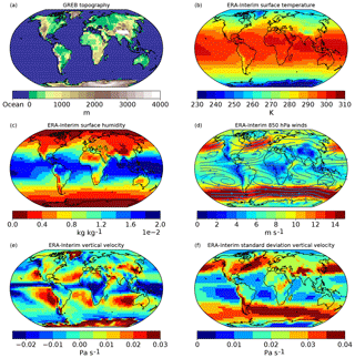
Figure 1 GREB mean state boundary conditions and reference climatologies: topography (a), surface temperature (b), surface humidity (c), 850 hPa wind direction (streamline) and strength (shading) (d), vertical velocity ω (e) and the daily standard deviation of vertical velocity ω (f).

The observed hydrological cycle in terms of the annual mean and its seasonal cycle (DJF minus JJA) for precipitation, evaporation and moisture circulation are shown in Figs. 2 and 3. The global pattern of precipitation is marked by the ITCZ, its seasonal cycle and by the storm tracks of the midlatitudes. The evaporation is strongest over subtropical oceans and has a complex seasonal cycle with generally more evaporation in the warm season over land. The horizontal moisture transport (Figs. 2c and 3c) is dominated by large-scale convergence and divergence zones over the oceans and their seasonal shift.

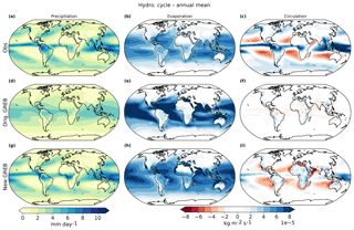
Figure 2 The decomposition of the hydrological cycle into its parts: precipitation in mm day⁻¹ (a, d, g), evaporation (b, e, h) and circulation in kg m⁻² s⁻¹ (c, f, i) in observations (a, b, c), the original GREB model (d, e, f) and the new GREB model (g, h, i) for the annual mean.

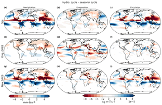
Figure 3 As Fig. 2 but for the seasonal cycle (DJF–JJA). The decomposition of the hydrological cycle into its parts: precipitation in mm day⁻¹ (a, d, g), evaporation (b, e, h) and circulation in kg m⁻² s⁻¹ (c, f, i) in observations (a, b, c), the original GREB model (d, e, f) and the new GREB model (g, h, i) for the seasonal cycle.

Model simulations, pre-industrial (pi-Control) and Representative Concentration Pathways 8.5 (RCP8.5) from the CMIP5 database are used for comparison (Taylor et al., 2012). All data sets are regridded to a horizontal resolution of $\mathrm{3.75}{}^{\circ }\times \mathrm{3.75}{}^{\circ }$ to match the GREB model grid. See Table 1 for a complete list of models used.

Table 1 List of CMIP5 models.

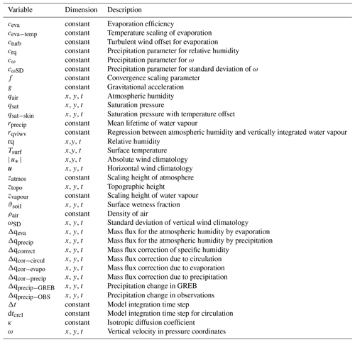
The original GREB hydrological cycle model, which is the starting point for this study, is shortly presented below. All variables and parameters are listed and explained in Table 2. The precipitation is proportional to the specific humidity,

$$\begin{array}{}\text{(1)}& {\displaystyle }\mathrm{\Delta }{q}_{\mathrm{precip}}=r_{\mathrm{precip}}\cdot q_{\mathrm{air}},\end{array}$$

with Eq. (1), which corresponds to an autoregressive model with a decorrelation (recirculation) time of about 14 days (Dommenget and Floter, 2011). Evaporation, Δq_eva, in the original GREB model is calculated using an extended bulk formula:

$$\begin{array}{}\text{(2)}& {\displaystyle }\mathrm{\Delta }{q}_{\mathrm{eva}}={\displaystyle \frac{{\mathit{\rho }}_{\mathrm{air}}\cdot c_{\mathrm{w}}\cdot \left|u_{*}+c_{\mathrm{turb}}\right|\cdot {\mathit{\vartheta }}_{\mathrm{soil}}\cdot \left(q_{\mathrm{air}}-q_{\mathrm{sat}}\right)}{r_{\mathrm{qviwv}}}}.\end{array}$$

The bulk formula depends on the saturation deficit (q_air−q_sat), the wind speed u_*, with a turbulent wind factor (c_turb), the density of air (ρ_air), the transfer coefficient (c_w) and a linear regression factor (r_qviwv), which links surface humidity to the vertically integrated water vapour column (Dommenget and Floter, 2011; Rapti, 2005).

Table 2 Variables of the GREB model.

The saturation water vapour pressure is calculated after (Dommenget and Floter, 2011; James, 1995)

$$\begin{array}{}\text{(3)}& {\displaystyle }{q}_{\mathrm{sat}}=e^{\frac{z_{\mathrm{topo}}}{z_{\mathrm{atmos}}}}\cdot \mathrm{3.75}\times {\mathrm{10}}^{-\mathrm{3}}\cdot e^{\mathrm{17.08085}\cdot \frac{T_{\mathrm{surf}}-\mathrm{273.15}}{T_{\mathrm{surf}}-\mathrm{38.975}}}.\end{array}$$

Together, this leads to the complete tendency equation of specific humidity in GREB:

$$\begin{array}{}\text{(4)}& {\displaystyle \frac{\mathrm{d}{q}_{\mathrm{air}}}{\mathrm{d}t}}=\mathrm{\Delta }{q}_{\mathrm{eva}}+\mathrm{\Delta }{q}_{\mathrm{precip}}+\mathit{\kappa }\cdot {\mathrm{\nabla }}^{\mathrm{2}}{q}_{\mathrm{air}}-\mathit{u}\cdot \mathrm{\nabla }{q}_{\mathrm{air}}+\mathrm{\Delta }{q}_{\mathrm{correct}},\end{array}$$

with the diffusion term, κ⋅∇²q_air, the advection term, u⋅∇q_air, and the flux correction term, Δq_correct. The simulated annual mean and seasonal cycle for precipitation, evaporation and mean horizontal moisture transport are shown in Figs. 2 and 3 for the original GREB model as discussed above. The diffusion term is only one-fifth of the magnitude of the advection term in global average (not shown) but is more important in some locations and therefore not ignored in the GREB model. The original GREB model simulated some of the main features of the regional differences in the precipitation and evaporation, but many important details are missing (e.g. ITCZ, subtropical dry regions or extratropical storm tracks). However, horizontal moisture transport is not simulated well by the original GREB model.

The seasonally varying flux correction term, Δq_correct, is calculated as the residual between the tendencies without flux corrections and observed tendencies:

$$\begin{array}{ll}{\displaystyle }& {\displaystyle }\mathrm{\Delta }{q}_{\mathrm{correct}}={\left.{\displaystyle \frac{\mathrm{d}{q}_{air}}{\mathrm{d}t}}\right|}_{\mathrm{obs}}-\mathrm{\Delta }{q}_{\mathrm{eva}}+\mathrm{\Delta }{q}_{\mathrm{precip}}\\ \text{(5)}& {\displaystyle }& {\displaystyle }+\mathit{\kappa }\cdot {\mathrm{\nabla }}^{\mathrm{2}}{q}_{\mathrm{air}}-\mathit{u}\cdot \mathrm{\nabla }{q}_{\mathrm{air}}.\end{array}$$

This effectively corrects the GREB model to have a climatological specific humidity as observed. The flux correction term, Δq_correct, can help to evaluate the improvements in the hydrological cycle model. The better the model the smaller the correction term should be in Eq. (4). We can therefore split the flux correction into three diagnostic terms:

$$\begin{array}{}\text{(6)}& {\displaystyle }\mathrm{\Delta }{q}_{\mathrm{correct}}=\mathrm{\Delta }{q}_{\mathrm{cor}-\mathrm{precip}}+\mathrm{\Delta }{q}_{\mathrm{cor}-\mathrm{evapo}}+\mathrm{\Delta }{q}_{\mathrm{cor}-\mathrm{circul}},\end{array}$$

with each term on the right-hand side representing the fraction of the flux corrections attributed to precipitation, evaporation and circulation biases, respectively. Each term is estimated as the difference between the observed and the GREB model tendencies of the humidity resulting from precipitation, evaporation and circulation biases:

$$\begin{array}{}\text{(7)}& {\displaystyle }& {\displaystyle }\mathrm{\Delta }{q}_{\mathrm{cor}-\mathrm{precip}}=\mathrm{\Delta }{q}_{\mathrm{precip}-\mathrm{OBS}}-\mathrm{\Delta }{q}_{\mathrm{precip}-\mathrm{GREB}}\text{(8)}& {\displaystyle }& {\displaystyle }\mathrm{\Delta }{q}_{\mathrm{cor}-\mathrm{evapo}}=\mathrm{\Delta }{q}_{\mathrm{evapo}-\mathrm{OBS}}-\mathrm{\Delta }{q}_{\mathrm{evapo}-\mathrm{GREB}}\text{(9)}& {\displaystyle }& {\displaystyle }\mathrm{\Delta }{q}_{\mathrm{cor}-\mathrm{circul}}=\mathrm{\Delta }{q}_{\mathrm{circul}-\mathrm{OBS}}-\mathrm{\Delta }{q}_{\mathrm{circul}-\mathrm{GREB}},\end{array}$$

with the GREB model tendencies of the humidity resulting from circulation, Δq_{circul−GREB}, defined as

$$\begin{array}{}\text{(10)}& {\displaystyle }\mathrm{\Delta }{q}_{\mathrm{circul}}=\mathit{\kappa }\cdot {\mathrm{\nabla }}^{\mathrm{2}}{q}_{\mathrm{air}}-\mathit{u}\cdot \mathrm{\nabla }{q}_{\mathrm{air}}.\end{array}$$

The observed humidity tendencies resulting from circulation, Δq_{circul−GREB}, are defined by the residual of the total humidity tendency minus the precipitation and evaporation tendencies. By construction, all three flux correction terms (evaporation, precipitation and circulation) sum up to the total flux correction term.

3 Hydrological cycle model development

The development of the new hydrological cycle model of the GREB model is based on the existing zero-order hydrological cycle model of the GREB model. The following section outlines the development of each of the three models and discusses how the change in the reference climatologies from NCEP to ERA-Interim has affected the model. All variables are summarised in Table 2.

3.1 Precipitation

The original GREB precipitation model captures some large-scale aspects of the mean and seasonal cycle of observed precipitation, such as more precipitation in the tropics and during warm seasons over land (Figs. 2 and 3). It has, however, substantial differences from the observed precipitation, as it cannot capture the high rainfall in the ITCZ and the enhanced precipitation over the midlatitude storm track regions, and misses many aspects of the seasonal cycle. The root mean square error for the annual mean of the original GREB model precipitation parameterisation is 1.46 mm day⁻¹.

The new parameterisation of precipitation in the GREB model is assumed to be proportional to q_air, as in the original GREB model. We further assume that relative humidity, rq, and upward air motion, ω, increase rainfall. The latter is assumed to be a function of the mean and the standard deviation of the daily mean variation, ω_mean and ω_SD, respectively. The new precipitation parameterisation is

$$\begin{array}{ll}{\displaystyle }& {\displaystyle }\mathrm{\Delta }{q}_{\mathrm{precip}}\\ \text{(11)}& {\displaystyle }& {\displaystyle }=r_{\mathrm{precip}}\cdot q_{\mathrm{air}}\cdot \left(c_{\mathrm{rq}}\cdot \text{rq}+c_{\mathit{\omega }}\cdot {\mathit{\omega }}_{\mathrm{mean}}+c_{\mathit{\omega }\text{SD}}\cdot {\mathit{\omega }}_{\mathrm{SD}}\right).\end{array}$$

The model parameters, r_precip, c_rq, c_ω and c_ωSD, are fitted to minimise the root mean square error (RMSE) between observations and GREB simulated precipitation. The resulting mean precipitation and its seasonal cycle are shown in Figs. 2g and 3g. The model is evaluated in a Taylor diagram in Fig. 4a and d against observations. The new GREB precipitation model is now very close to the observed precipitation patterns in both the mean and annual cycles. It is actually closer to the observed precipitation than any CMIP5 model (Fig. 4a and d). We further test the different elements of the precipitation model by only considering a subset of the variables in Eq. (11), setting the other terms to zero and fitting the parameterisations for these reduced models. This allows us to estimate the effect of each term in the equation; see Figs. 4a, d and 5.

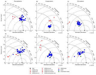
Figure 4 Precipitation (a, d), evaporation (b, e) and circulation (c, f) in the annual mean (a, b, c) and seasonal cycle (d, e, f) in mm day⁻¹ in a Taylor diagram against observations from GPCP and ERA-Interim. Red colours indicate different GREB parameterisations, with 0 being the original and red ★ the best parameterisation. Blue dots are pi-Control CMIP5 models, and the green cross indicates the ensemble mean of all CMIP5 models.

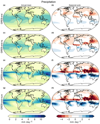
Figure 5 Annual mean precipitation for four development steps of the GREB precipitation parameterisation (a, c, e, g) and their corresponding seasonal cycles (b, d, f, h) in mm day⁻¹ . The first step was changing the specific humidity boundary climatology (a, b). Then subsequently more variables have been added to the precipitation parameterisation: adding only relative humidity (c, d), adding only ω (e, f), adding relative humidity and ω (g, h).

Relative humidity (rq) is widely used in climate models as a predictor for precipitation (Petoukhov et al., 1999, 2005; Wang and Myask, 2000; Weaver et al., 2001). In the GREB model, it increases precipitation mainly over humid regions such as the Amazon Basin (Fig. 5c) and amplifies the seasonal cycle (Fig. 5d). The overall pattern of rainfall with high precipitation in the tropics and decreasing towards higher latitudes is not changed. Including rq gives some moderate improvement relative to the original GREB model (Fig. 4a comparing marker “0” to marker “b”).

The mean vertical air motion (ω_mean) provides a substantial improvement of the precipitation model (Fig. 4a and d comparing marker “0” to “c”). Ascending air masses in the ITCZ lead to increased precipitation, whereas descending air masses (i.e. in the subtropics) suppress precipitation. It creates a sharper and more realistic gradient in precipitation than the original GREB model (compare Figs. 2d and 5e). With the addition ω_mean, GREB is in the range of uncertainty of more complex CMIP5 models in the annual mean and the seasonal cycle (Fig. 4a and d).

The GREB precipitation model without ω_SD has still fairly weak mean precipitation in the midlatitude storm track regions (compare Figs. 5g and 2g) and has a weak seasonal cycle with the wrong sign in these regions as well (compare Figs. 5h and 3g). The transient pressure systems in these regions lead to large vertical motions (ω) on shorter, daily timescales that result in large precipitation but have a near-zero ω_mean. Thus, to capture the precipitation in regions with strong variability in ω, but weak ω_mean, we include ω_SD. This mainly enhances rainfall in the midlatitudes and high latitudes (Figs. 2g and 3g).

In summary, the new GREB precipitation model is significantly better than the original model. The RMSE is reduced by 0.65 to 0.81 mm day⁻¹ in the annual mean and by 1 mm day⁻¹ in the seasonal cycle. GREB precipitation now has a comparable skill to more complex CGCMs and lies within the range of uncertainty of CMIP5 modelled precipitation. Introducing the new precipitation parameterisation globally reduces the flux corrections of specific humidity caused by precipitation; see Fig. 6c and d. The root mean square of the flux corrections caused by precipitation is reduced by more than 40 %, indicating that the new parameterisation has indeed improved the simulation of the hydrological cycle in the GREB model. Similar improvements are gained for the seasonal cycle (Fig. 7c and d). The original GREB model showed large flux corrections, especially in the tropics where the ITCZ moves with seasons and in the midlatitudes. The pattern of the flux corrections of the new model still looks similar to the original model but is only half as large in amplitude (Figs. 6c, d and 7c, d).

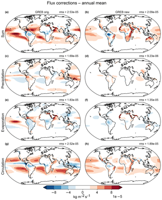
Figure 6 Annual mean flux corrections of specific humidity for the original GREB model (a) and the improved GREB model (b). The flux corrections are then split into their contributions of precipitation (c, d), evaporation (e, f) and circulation (g, h) for the original GREB model (a, c, e, g) and the improved GREB model (b, d, f, h) in kg m⁻² s⁻¹. The top right corner of each panel shows the global root mean square (rms).

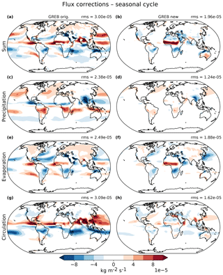
Figure 7 As Fig. 6 but for the seasonal cycle (DJF minus JJA). Flux corrections of specific humidity for the original GREB model (a) and the improved GREB model (b). The flux corrections are then split into their contributions of precipitation (c, d), evaporation (e, f) and circulation (g, h) for the original GREB model (a, c, e, g) and the improved GREB model (b, d, f, h) in kg m⁻² s⁻¹. The top right corner of each panel shows the global rms.

3.2 Evaporation

In the original GREB model, evaporation is calculated using a widely used bulk formula approach (see Eq. 1 in Richter and Xie, 2008). This model does capture the main aspects of the regional differences in the annual mean evaporation in GREB, with enhanced evaporation over subtropical oceans and weaker evaporation over land (Fig. 2e). The seasonal cycle (Fig. 3e) is, however, very different from observed, and the land–sea differences are too strong.

For the new evaporation model, we retained the original bulk formula approach and included a few minor changes by considering land–sea differences, revised wind (u_*) estimates, scaled effectivity and skin temperature. The new evaporation model is

$$\begin{array}{ll}{\displaystyle }& {\displaystyle }\mathrm{\Delta }{q}_{\mathrm{eva}}\\ \text{(12)}& {\displaystyle }& {\displaystyle }={\displaystyle \frac{{\mathit{\rho }}_{\mathrm{air}}\cdot c_{\mathrm{eva}}\cdot c_{\mathrm{w}}\cdot \left|u_{*}+c_{\mathrm{turb}}\right|\cdot {\mathit{\upsilon }}_{\mathrm{soil}}\cdot \left(q_{\mathrm{air}}-q_{\mathrm{sat}-\mathrm{skin}}\right)}{r_{\mathrm{qviwv}}}}.\end{array}$$

The constant c_eva modifies the evaporation efficiency for a given mean wind speed, u_*. q_sat−skin is an estimate of saturated humidity considering skin temperature. It is calculated using

$$\begin{array}{ll}{\displaystyle }& {\displaystyle }{q}_{\mathrm{sat}-\mathrm{skin}}\\ \text{(13)}& {\displaystyle }& {\displaystyle }=e^{\frac{z_{\mathrm{topo}}}{z_{\mathrm{atmos}}}}\cdot \mathrm{3.75}\times {\mathrm{10}}^{-\mathrm{3}}\cdot e^{\mathrm{17.08085}\cdot \frac{T_{\mathrm{surf}}+c_{\mathrm{eva}-\mathrm{temp}}-\mathrm{273.15}}{T_{\mathrm{surf}}+c_{\mathrm{eva}-\mathrm{temp}}-\mathrm{38.975}}}.\end{array}$$

The parameter c_eva−temp is a constant temperature offset to mimic skin temperature difference to T_surf. The parameters c_eva, c_eva−temp and c_turb are fitted against observations for ocean and land points individually to minimise the RMSE. The values we estimated are

$$\begin{array}{}\text{(14)}& {\displaystyle }{c}_{\mathrm{eva}}& {\displaystyle }=\left\{\begin{array}{l}\mathrm{0.25}\text{over land}\\ \mathrm{0.58}\text{over ocean}\end{array}\right.\text{(15)}& {\displaystyle }{c}_{\mathrm{eva}-\mathrm{temp}}& {\displaystyle }=\left\{\begin{array}{l}\mathrm{5}\text{K over land}\\ \mathrm{1}\text{K over ocean}\end{array}\right.\text{(16)}& {\displaystyle }{c}_{\mathrm{turb}}& {\displaystyle }=\left\{\begin{array}{l}\mathrm{11.5}\text{over land}\\ \mathrm{5.4}\text{over ocean}\end{array}\right.\end{array}$$

The scaled effectivity (c_eva) is lower over land than over oceans reflecting the fact that for a given u_∗ more evaporation is simulated over oceans. This appears to be realistic considering that land has lower wind speeds near the surface for a given u_* due to the topography and vegetation. The value of c_eva⋅c_w closely matches the observed values over oceans (Anderson and Smith, 1981; Merlivat, 1978).

The skin temperature difference approximated by c_eva−temp is larger over land. It reflects that the GREB model does not simulate the daily cycle, and the larger daily cycle over land leads to an effectively larger difference between the simulated T_surf and the skin temperature. The offset of 1 ^∘C over oceans is also found by Feng et al. (2018).

The wind magnitudes (u_*) in the original GREB model were estimated on the basis of the monthly mean climatologies of the zonal and meridional wind components. This, however, is not an accurate estimate of the monthly mean wind magnitudes, as it neglects the turbulent term due to high frequent variability. In the new GREB model, we estimate the monthly mean u_* climatology based on the original 6-hourly ERA-Interim time steps.

We can estimate how much each of these changes improved the evaporation model by including only one of these changes and fitting the parameters of these models individually; see Figs. 4b, e and 8.

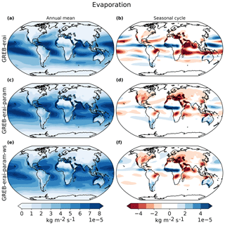
Figure 8 Annual mean evaporation for three development steps of the GREB evaporation parameterisation (a, c, e) and their corresponding seasonal cycles (b, d, f) in kg m⁻² s⁻¹. The first step was changing the boundary climatology (a, b). Then subsequently more variables have been added to the evaporation parameterisation: fitting the evaporation parameters separately for ocean and land (c, d) and fitting parameters and prescribing the wind speed (e, f).

Fitting the evaporation efficiency c_eva and the turbulent wind factor improves evaporation over land, especially in the seasonal cycle (Fig. 8d), and reduces the strength of evaporation over the ocean. The increase in evaporation over land is caused by the increase in the turbulent wind factor. c_eva would decrease the evaporation in the annual mean and the seasonal cycle. By including the new estimate of monthly mean wind speed u_*, the pattern of evaporation is getting closer to observations, especially over the oceans (i.e. Fig. 8f, North Atlantic), and by including the new estimate of skin temperature the seasonal cycle is improving slightly (Fig. 4e).

The original GREB model was evaporating too much on the annual mean (see Fig. 2e) especially over the equatorial Pacific and Atlantic. The new hydrological cycle model parameterisation largely decreases evaporation over these regions and the flux corrections are reduced over the globe in the annual mean (Fig. 6e, f). The correlation of the annual mean experiences the largest changes from changing the reference climatology (Fig. 4b).

In the seasonal cycle, each included variable improves the simulation of evaporation in the GREB model (Fig. 4e). The seasonal cycle of flux corrections caused by evaporation in the original GREB model is large over land and large over oceans. There are positive flux corrections around the Equator and negative flux corrections over the oceans north of the Equator (Fig. 7e). The improved evaporation seasonal cycle mainly removes this distinct pattern over the oceans and reduces flux corrections over most land areas. (Fig. 7e, f). Overall, the new evaporation model is slightly better than in the original GREB model, but it still has substantial limitation in simulating the seasonal cycle correctly (Figs. 2h, 3h).

3.3 Transport

The original GREB model transport of moisture was very weak and had little agreement with observations (Figs. 2f and 3f). Atmospheric transport of moisture in GREB (Eq. 4) is controlled by diffusion and advection with mean winds. This model considered a divergence free two-dimensional flow.

However, moisture convergence, as it occurs, for example, in the ITCZ, is important for the transport of moisture in these regions. The mean convergence by advection including the moisture convergence term is

$$\begin{array}{}\text{(17)}& {\displaystyle }\stackrel{\mathrm{‾}}{\mathbf{\nabla }\left(\mathit{u}\cdot q_{\mathrm{air}}\right)}=\stackrel{\mathrm{‾}}{\mathit{u}\cdot \mathbf{\nabla }{q}_{\mathrm{air}}}+\stackrel{\mathrm{‾}}{q_{\mathrm{air}}\cdot \mathbf{\nabla }\mathit{u}}.\end{array}$$

The second term on the right-hand side was not considered in the original GREB model but is now considered in the new model. The moisture convergence term can be approximated by knowing the vertical air flow assuming continuity and hydrostatic balance:

$$\begin{array}{}\text{(18)}& {\displaystyle }\stackrel{\mathrm{‾}}{q_{\mathrm{air}}\cdot \mathbf{\nabla }\mathit{u}}\approx q_{\mathrm{air}}\cdot f\cdot {\displaystyle \frac{\mathrm{d}{t}_{\mathrm{crcl}}}{z_{\mathrm{vapour}}\cdot {\mathit{\rho }}_{\mathrm{air}}\cdot g}}\cdot \left(-\mathit{\omega }\right),\end{array}$$

with the known parameters scaling height of water vapour, z_vapour, density of air, ρ_air, gravitational acceleration, g, and the circulation time step, dt_crcl. The scaling factor, f, should theoretically be 1.0, but the mean large-scale horizontal winds and vertical velocities may not perfectly match because of the coarse horizontal resolution. Other factors that influence f could be the single-layer approximation, the GREB scaling height of water vapour that is larger than literature values or calculating the reference circulation as residual. A fit of Eq. (18) to observations finds that f=2.5.

This new model has now fairly realistic transport in the annual mean and the seasonal cycle (Figs. 2i and 3i), with clear moisture transport out of regions with diverging flow (e.g. in the subtropics off the coast of Peru) and into converging zones (e.g. ITCZ). The new parameterisation of convergence also reduces the flux corrections in the annual mean and the seasonal cycle (Figs. 6g, h and 7g, h).

3.4 Boundary conditions and input data

The original GREB model used the NCEP reanalysis as boundary conditions and as references for estimating the parameterisation of the model. New generations of reanalysis products have improved, because of the use of better models, better input data and better assimilation products (Dee et al., 2011). This is shown by Chen (2016), who investigated the variability and trends of the vertically integrated water vapour and found that ECMWF's ERA-Interim reanalysis has a higher accuracy than NCEP and a better agreement with observations over oceans and in the tropics. NCEP underestimates water vapour in troposphere (Kishore et al., 2011). We therefore changed the reference climatology of specific humidity in the GREB model from NCEP to ERA-Interim. To get a consistent model, we also take surface temperature, horizontal winds, the climatology of ω and standard deviation of ω from ERA-Interim. The effect of changing the mean climatology from the years 1950–2008 to 1979–2015 is small compared to the differences between NCEP and ERA-Interim. The parameters of our new GREB hydrological cycle model are then fitted against the new reference climatologies.

We estimate the effect that the change in reference climatologies will have on the new GREB hydrological cycle model by fitting the parameters of the new model as described above to both the NCEP and ERA-Interim reanalysis. The resulting hydrological cycle models are evaluated against observations (GPCP and ERA-Interim) in Taylor diagrams for the annual mean. Changing the reference climatology does not lead to major improvements in the representation of the hydrological cycle in the GREB model, but it increases the correlation of precipitation, evaporation and circulation and reduces the RMSE (Fig. S1 in the Supplement). The main improvement is in the tropics and might be related to the underestimated value of specific humidity in the tropics found by Chen (2016) and Kishore et al. (2011).

4 Model verification

We now test the new hydrological model in a series of three different sensitivity experiments. The discussion focuses on evaluating the new model. The three examples test the hydrological cycle model response to changes in the boundary conditions. These changes are beyond those used to fit the model parameterisation and can therefore be a test of the model's skill. We will leave more in-depth analysis of some of these experiments to future studies.

4.1 Seasonal cycle

The response of the hydrological cycle to seasonal changes is a good test for evaluating the skill of the hydrological cycle model. The GREB model applies monthly flux correction terms to maintain a mean atmospheric humidity as observed. Thus, by construction, the specific humidity in each calendar month in the GREB model is identical to the observations; see Fig. 9a.

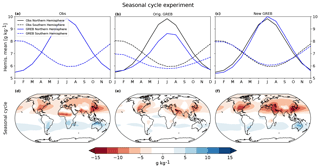
Figure 9 Annual cycle of specific humidity with seasonal varying flux corrections (a, d) and annual mean flux corrections for original GREB (b, e) and improved GREB (c, f) in g kg⁻¹. The top row shows the northern (solid) and southern (dashed) hemispheric mean for observations (black) and GREB (blue). The bottom row shows the respective seasonal cycle (DJF minus JJA). For the seasonally varying flux corrections (a), GREB (blue) matches observations (black).

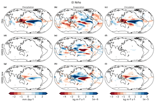
Figure 10 The El Niño response of the hydrological cycle in observations for precipitation (a) in mm day⁻¹, evaporation (b) and circulation (c) in kg m⁻² s⁻¹, original GREB model for precipitation (d), evaporation (e) and circulation (f) and the improved GREB model for precipitation (g), evaporation (h) and circulation (i). GREB uses prescribed anomalies from an El Niño composite mean of surface temperature, horizontal winds and vertical winds (ω).

To illustrate that the seasonal cycle is not a feature of the seasonally varying flux corrections, we changed the flux corrections to an annual mean value for the original GREB model (Fig. 9b, e) and for the new GREB model (Fig. 9c, f). This annual mean flux correction value is added on every time step to the tendency equation of specific humidity (Eq. 4).

With the new parameterisations for precipitation, evaporation and circulation, the new GREB model resolves the seasonal cycle better than the original GREB model (Fig. 9). The seasonal cycle of the original GREB model was too weak in the Northern Hemisphere when compared to observations, and throughout the year the GREB model was too dry (Fig. 9b). For the Southern Hemisphere, the original GREB model was too wet. The new GREB model captures the high humidity in northern hemispheric summer and the low values in winter (Fig. 9c). This makes the seasonal cycle stronger in the new GREB model and it is closer to the reference climatology. In summary, the new GREB hydrological cycle model simulates the seasonal evolution of the atmospheric humidity very well and significantly better than the original GREB model.

4.2 El Niño–Southern Oscillation

Strong El Niño and La Niña events lead to significant changes in the tropical precipitation and associated hydrological cycle changes. Since these natural modes of climate variability are well documented, they present a good test case for the GREB model.

We therefore conducted a set of sensitivity experiments with the GREB model forced by the mean conditions for strong El Niño and La Niña events. The GREB model was forced with mean composites of T_surf, horizontal winds and ω from observations for four El Niño (1982/83, 1987/88, 1991/92, 1997/98) and La Niña (1988/89, 1999/2000, 2007/08, 2010/11) events. The anomalies are calculated around El Niño/La Niña from May before the peak in December to April in the following year and against the climatological mean. In the GREB model simulation, they are added on top of the reference climatology. The observed anomalies in the hydrological cycle during these El Niño events are shown in Fig. 10a–c. The skill of simulating La Niña events are qualitatively the same. We clearly note strong regional changes in the precipitation in the tropical Pacific that match changes in moisture transport (Fig. 10c), illustrating that El Niño–Southern Oscillation (ENSO) events mark strong regional changes in the hydrological cycle related to changes in the circulation.

The new GREB response in precipitation shows a strong similarity with the observed changes (Fig. 10g). There is a shift of rainfall from the Maritime Continent towards the NINO3.4 region (5^∘ N to 5^∘ S and 170 to 120^∘ W) over the Pacific. However, the overall amplitude in the precipitation response is in general weaker than observed. In contrast, the original GREB model has nearly no precipitation response to the ENSO forcings. This is consistent with the weak response in the circulation in the original GREB model (Fig. 10f). The correlation between the GREB-simulated El Niño response increases from 0.0 for the original GREB model to 0.9 with the new GREB model.

The observed evaporation response to ENSO events in the tropical Pacific somewhat counteracts the precipitation response, as we observe mostly decreased evaporation over regions with enhanced precipitation and increased evaporation over regions with reduced precipitation (Fig. 10a and b). These evaporation changes are mostly caused by changes in winds, with decreased evaporation over regions where the winds have weakened (e.g. NINO3.4 region). The new GREB model somewhat captures this pattern but shows a stronger evaporation response, which partly explains the weaker precipitation response. However, both the original and the new GREB model evaporation simulations have only a weak spatial correlation (0.3) with the observed evaporation changes overall.

The observed strong changes in the circulation of atmospheric humidity (Fig. 10c) is mostly due to changes in the convergence of moisture (e.g. ω). Since convergence of moisture was not considered in the original GREB model, the simulated changes in the circulation are very weak in the original GREB model (Fig. 10f). The new GREB model does consider convergence of moisture and simulates the changes in the circulation of atmospheric humidity very similarly to the observed (Fig. 10i). The new circulation parameterisation in the new GREB model improves the correlation between the observed and the simulated circulation tendency from 0.3 (original GREB) to 0.95.

In summary, the new GREB model does simulate the precipitation and circulation response to ENSO conditions fairly well, whereas the original GREB model has very little skill, illustrating the significant improvement of the new GREB model over the original GREB model. However, the evaporation response in both models is not as well simulated as the precipitation and circulation responses.

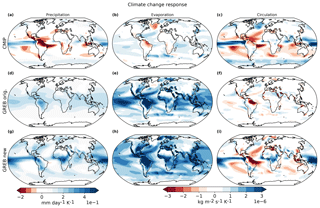
Figure 11 Response of the hydrological cycle to an RCP8.5 forcing in the CMIP5 ensemble mean for precipitation (a) in mm day⁻¹, evaporation (b) and circulation (c) in kg m⁻² s⁻¹, original GREB model for precipitation (d), evaporation (e) and circulation (f) and the improved GREB model for precipitation (g), evaporation (h) and circulation (i). GREB uses prescribed anomalies from the CMIP5 ensemble mean of surface temperature, horizontal winds and vertical winds (ω). All responses are shown per degree of warming.

4.3 Global warming

The response of the hydrological cycle to global warming is one of the potential applications of the GREB model and a comparison of the GREB model with the CMIP model simulations response to global warming provides a good test. The CMIP5 ensemble mean response of precipitation shows a distinct increase of rainfall in the equatorial Pacific, decreases of mean rainfall in some subtropical regions (i.e. east Pacific) and increases in some areas of the midlatitudes; see Fig. 11a. This pattern is normally referred to as the wet-get-wetter paradigm (Held and Soden, 2006). Although this approach has been questioned by more recent studies (Chadwick et al., 2013), it is still a good first-order approach to the changes in the global hydrological cycle, although changes over land might be muted or even reversed (He and Soden, 2016).

To evaluate the GREB hydrological cycle model independent of the other GREB model components, such as the T_surf tendencies, we force the original and new GREB models with RCP8.5 equivalent CO₂ concentrations and all other input variables for the hydrological cycle model taken from CMIP model simulations. That is, we add T_surf, horizontal winds and vertical velocity RCP8.5 CMIP5 ensemble mean anomalies from the models described in Table 1 on top of the GREB control reference climatologies. In the control run, the reference boundary conditions of T_surf, horizontal winds and ω are taken.

The precipitation response in the original GREB model is positive in all locations and it closely follows the pattern of specific humidity in the control simulation (see Eq. 1 and Fig. 11d). This is mainly due to an increase in the saturation water vapour pressure of about 7 % per degree of warming (Clausius–Clapeyron). The original GREB precipitation response pattern is not correlated to the CMIP5 ensemble mean response pattern (Fig. 12a), suggesting that local differences in the precipitation response are very different from those in the CMIP simulations.

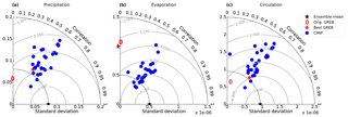
Figure 12 RCP8.5 response of CMIP5 models (blue), original GREB (0) and improved GREB (red ★) per degree of global warming against the CMIP5 ensemble mean (black star). Precipitation (a), evaporation (b) and circulation (c) are shown. GREB uses prescribed anomalies from the CMIP5 ensemble mean of surface temperature, horizontal winds and vertical winds (ω). The correlation of the original GREB model precipitation response with the ensemble mean is zero. The original and improved GREB models have zero correlation with the ensemble mean evaporation and the standard deviation is 1 for both.

The improved GREB model response pattern is similar to the CMIP models with enhanced and reduced response roughly at similar locations, which leads to a much improved correlation (Fig. 12a and c). This is strongly related to the moisture transport changes. However, the overall global mean precipitation response in the new GREB model is shifted upwards compared to the CMIP5 ensemble mean, which is related to the much stronger response in evaporation (compare Fig. 11b and h). In CMIP5 models, we see a muted response of evaporation mainly due to changes in surface relative humidity and surface stability (Richter and Xie, 2008).

5 Summary and discussion

In this study, we introduced the newly developed hydrological cycle model for the GREB model. It consists of three parts: precipitation, evaporation and transport. The development of these models started from the existing zero-order hydrological cycle model of the GREB model and used physical reasoning and observations for fitting parameters.

The simulation of precipitation and transport of moisture in the new hydrological cycle model is now comparable in skill to CMIP models in terms of annual mean and the seasonal cycle of rainfall. The simulation of precipitation in the GREB model is closer to the observed precipitation pattern than any CMIP5 model in both the annual mean and the seasonal cycle. This is directly related to the fact that the GREB mode has a prescribed atmospheric circulation, which is the main driver of the global precipitation pattern.

The evaporation has only improved slightly but does simulate the annual mean values fairly well. However, it is still different from the observed seasonal cycle and the skill is much lower than that of the CMIP model. This suggests that the evaporation model is still a limiting factor in the GREB model.

We applied the new hydrological cycle model to a number of sensitivity studies, which illustrated that the new hydrological cycle model is much improved over the original GREB model. The annual cycle simulation without any correction terms is very realistic with the new model, and the precipitation response to ENSO events is now very similar to the observed, due to the much-improved transport of moisture. Finally, the response to global warming now shows a precipitation response pattern that is comparable to that of the CMIP models. Again, a limiting factor in this sensitivity experiment was the evaporation response of the GREB model in comparison to that of CMIP models.

An interesting aspect of the GREB model is that it has the atmospheric circulation (vertical and horizontal winds), humidity and surface temperatures as boundary conditions. This allows the GREB model to be used as a diagnostic tool to understand how different boundary conditions affect aspects of the climate system, such as the hydrological cycle's response to global warming. It may also help to study how biases in the hydrological cycle in CMIP models related to different boundary conditions from the atmosphere, such as biases in the vertical winds. A recent study by Yang et al. (2018) links circulation biases in CMIP models to biases in precipitation and moisture. Forcing GREB with the circulation of CMIP models could shed light on how discrepancies in circulation between CMIP models affect the hydrological cycle. The new GREB hydrological cycle model is therefore a good tool in helping to conceptually understand the hydrological cycle and its response to global warming or other external forcings. It will further help in understanding CMIP model biases in the simulation of the hydrological cycle.