the Creative Commons Attribution 4.0 License.
the Creative Commons Attribution 4.0 License.
 | 25 Sep 2019
eSCAPE: Regional to Global Scale Landscape Evolution Model v2.0
Tristan Salles
The eSCAPE model is a Python-based landscape evolution model that simulates over geological time (1) the dynamics of the landscape, (2) the transport of sediment from source to sink, and (3) continental and marine sedimentary basin formation under different climatic and tectonic conditions. The eSCAPE model is open-source, cross-platform, distributed under the GPLv3 licence, and available on GitHub (http://escape.readthedocs.io, last access: 23 September 2019). Simulated processes rely on a simplified mathematical representation of landscape processes – the stream power and creep laws – to compute Earth's surface evolution by rivers and hillslope transport. The main difference with previous models is in the underlying numerical formulation of the mathematical equations. The approach is based on a series of implicit iterative algorithms defined in matrix form to calculate both drainage area from multiple flow directions and erosion–deposition processes. The eSCAPE model relies on the PETSc parallel library to solve these matrix systems. Along with the description of the algorithms, examples are provided to illustrate the model current capabilities and limitations. It is the first landscape evolution model able to simulate processes at the global scale and is primarily designed to address problems on large unstructured grids (several million nodes).
- Article
(27147 KB) - Full-text XML
- BibTeX
- EndNote


Since the 1990s, many software programmes have been designed to estimate long-term catchment dynamics, drainage evolution, and sedimentary basin formation in response to various mechanisms such as tectonic or climatic forcing (Braun and Sambridge, 1997; Coulthard et al., 2002; Davy and Lague, 2009; Simoes et al., 2010; Salles, 2016; Grieve et al., 2016b; Hobley et al., 2017). These models rely on a set of mathematical and physical expressions that simulate sediment erosion, transport, and deposition and can reproduce the 1st-order complexity of Earth's surface geomorphological evolution (Tucker and Hancock, 2010; Shobe et al., 2017).
In most of these models, climatic and tectonic conditions are imposed and often consist of rather simple forcing, such as uniform spatial precipitation and vertical displacements (uplift or subsidence), far from reflecting the complexity of the natural system. In addition, such approaches are unable to properly explore potential feedback mechanisms between each of the Earth's components. In fact, only a handful of these models are able to account more completely for the dynamics of the lithosphere and mantle, the role of sedimentation, and a more quantitative representation of climate relative to its interactions with topography (such as orographic rain) (Beaumont et al., 1992; Salles et al., 2011; Bianchi et al., 2015; Thieulot et al., 2014; Yang et al., 2015; Salles et al., 2017; Beucher et al., 2019). When made possible, it is often realised through the coupling of specialised numerical models involving the expertise of geodynamicists, geophysicists, and Earth's surface and atmospheric scientists.
Yet, we are still missing a tool to evaluate the global-scale evolution of the Earth's surface and its interaction with the atmosphere, the hydrosphere, and the tectonic and mantle dynamics. Such a tool will certainly provide new insights and help us to better characterise many aspects of the Earth system ranging from the role of atmospheric circulation in physical denudation, to the influence of the erosion and deposition of sediments on mantle convection, to the location and abundance of natural resources, to the evolution of life.
The model presented in this paper is a first step toward the development of a parallel global-scale landscape evolution model. It allows researchers to couple the Earth's surface with global climatic perturbations and geodynamic forces acting within the Earth's interior. Landscapes and sedimentary basin evolution in eSCAPE are driven by a series of standard stream power incision and diffusion laws (Howard et al., 1994; Tucker and Slingerland, 1997; Chen et al., 2014) designed to address problems from regional to global scales and over geological time (105–109 years). Due to the inherent assumptions made in the set of equations used, eSCAPE is not intended to estimate the evolution of individual fluvial channels but to quantify the large-scale and long-term evolution of Earth's surface regions (Salles et al., 2017; Armitage, 2019).
First, this paper presents the implicit, iterative approaches that are used to solve the multiple flow direction water routing and the erosion–deposition processes (Sect. 2). Then in Sect. 3, I provide a list of all the parameters required to run the eSCAPE model and I discuss the input and output formats. In addition, three examples based on both generic and global-scale experiments are described in detail and showcase the code main capabilities. Finally, in Sect. 4, I analyse the scalability of eSCAPE and discuss some of the limitations and future implementations that are necessary to improve the performance of the code on parallel architectures.
The eSCAPE model (Salles, 2018) is a parallel landscape evolution model built to simulate landscapes and basin dynamics at various space scales and timescales over unstructured grids. The model accounts for river incision using the stream power law, hillslope processes, and sediment transport in land and marine environments. It can be forced with spatially and temporally varying tectonics (horizontal and vertical displacements) and climatic forces (temporal and spatial precipitation changes and sea level fluctuations); eSCAPE is primarily written in Python with some functions in Fortran and takes advantage of PETSc solvers (Balay et al., 2012) over parallel computing architectures using a message-passing interface (MPI). In this section, I describe the simulated physical processes along with the algorithms that are used.
2.1 Implicit parallel flow discharge implementation
Flow accumulation (FA) calculations are a core component of landscape evolution models as they are often used as proxy to estimate flow discharge, sediment load, river width, bedrock erosion, and sediment deposition. Until recently, conventional FA algorithms were serial and limited to small spatial problems (O'Callaghan and Mark, 1984; Mark, 1988). With ever growing high-resolution digital elevation datasets, new methods based on parallel approaches have been proposed over the last decade. Due to the recursive nature of FA computation, graph traversal techniques are common in determining the upstream summation, and most approaches (Wallis et al., 2009; Wallace et al., 2010; Tarboton, 2013; Bellugi et al., 2011; Braun and Willett, 2013) are based on an initial ordering process followed by efficient priority-queue implementations with some variants, such as the sub-basin acyclic graph partitioning method in Salles and Hardiman (2016) or the breadth-first traversal approaches proposed by Barnes (2019). Except for the approach proposed by Barnes (2019), the previous methods scale well as long as the number of processors used is modest but quickly deteriorates as interprocessor communication costs increase.
In addition, when using the aforementioned implementation strategies, several problems might arise in (1) load balancing, when catchment size greatly changes in the simulated domain, or (2) handling very high resolutions at which multiple processes are needed for a single catchment. In addition, most of these methods assume a single flow direction (SFD – Fig. 1a). This assumption makes the emergent flow network highly sensitive to the underlying mesh geometry, and the dendritic shape of obtained stream networks is often an artefact of the surface triangulation. To reduce this effect, authors have proposed considering not only the steepest downhill direction but also representing other directions appropriately weighted by slope (multiple flow direction – MFD). Using MFD algorithms prevents the locking of erosion pathways along a single direction and helps to route flow over flat regions into multiple branches (Tucker and Hancock, 2010). Yet, graph traversal approaches cannot be easily modified to incorporate MFD algorithms as catchments are no longer strictly isolated in low-slope areas and flow pathways often diverge (Fig. 1b).
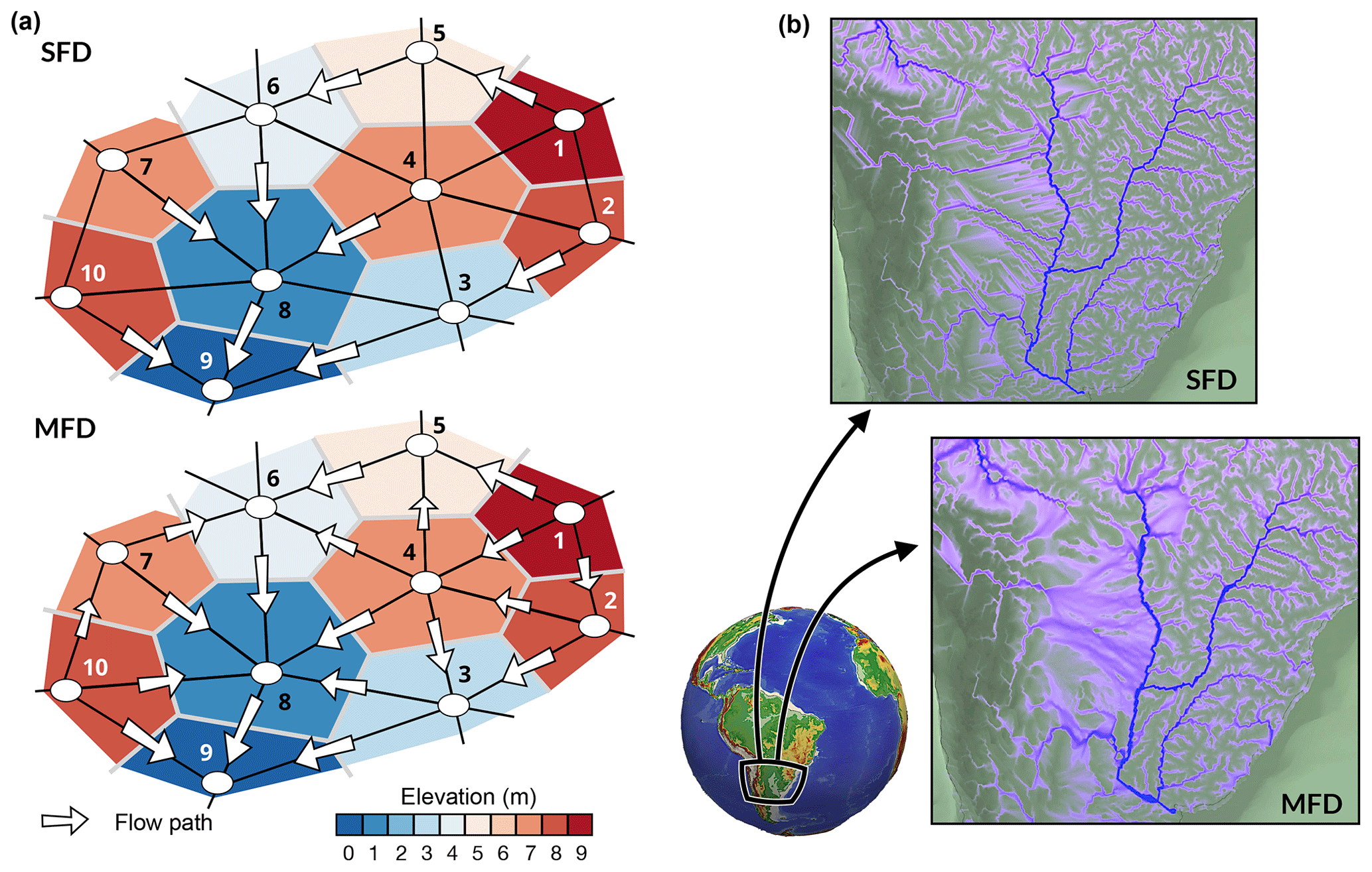
Figure 1(a) Schematic diagram showing flow paths when considering a triangular irregular network composed of 10 vertices (node IDs are given for each case). Cells (i.e. Voronoi area defining the region of influence of each vertex) are coloured by elevation. Two cases are presented considering single flow direction (top sketch – SFD) and multiple flow direction (bottom sketch – MFD ∕ D∞). White arrows indicate flow direction and their sizes vary in proportion to slope (not at scale). Node numbers correspond to the subscripts in Eqs. (2) and (4). (b) Differences in calculated drainage area for a portion of South America from eSCAPE using the two flow direction methods.
To overcome these limitations, Richardson et al. (2014) proposed using linear solvers. The approach consists of writing the FA calculation as a sparse matrix system of linear equations (Eddins, 2007; Schwanghart and Kuhn, 2010). It can take full advantage of purpose-built, efficient linear algebra routines including those provided by parallel libraries such as PETSc (Balay et al., 2012). The eSCAPE model computes the flow discharge (m3 yr−1) from FA and the net precipitation rate P using the parallel implicit drainage area (IDA) method proposed by Richardson et al. (2014) but adapted to unstructured grids (Fig. 1). The flow discharge at node i (qi) is determined as follows:
where bi is the local volume of water ΩiPi; Ωi is the Voronoi area and Pi the local precipitation value available for runoff during a given time step. Nd is the number of donors with a donor defined as a node that drains into i (as an example the donor of vertex 5 in the SFD sketch in Fig. 1a is 1). To find the donors of each node, the method consists of finding their receivers first. Then, the receivers of each donor are saved into a receiver matrix, noting that the nodes, which are local minima, are their own receivers. Finally, the transpose of the matrix is used to get the donor matrix. When Eq. (1) is applied to all nodes and considering the MFD case presented in Fig. 1a, the following relations are obtained:
The choice of weights wm,n depends on the number of flow directions used. The weights range between 0 and 1 and sum to 1for each node:
In eSCAPE, the number of flow direction paths is user defined and can vary from 1 (i.e. SFD) up to 12 (i.e. MFD) depending of the grid neighbourhood complexity. The weights are calculated based on the number of downslope neighbours and are proportional to the slope (Quinn et al., 1991; Tarboton, 1997; Richardson et al., 2014). In matrix form the system defined in Eq. (2) is equivalent to Wq=b or
The vector q corresponds to the unknown flow discharge (volume of water flowing on a given node per year) and the elements of W left blank are zeros.
As explained in Richardson et al. (2014), the above system is implicit as the flow discharge for a given vertex depends on its neighbours' unknown flow discharge. The matrix W is sparse and is composed of diagonal terms set to unity (identity matrix) and off-diagonal terms corresponding to at most the immediate neighbours of each vertex (typically fewer than six in constrained Delaunay triangulation).
In eSCAPE, this matrix is built in parallel using compressed sparse row matrix functionality available from SciPy (Jones et al., 2001). Once the matrix has been constructed, the PETSc library is used to solve matrices and vectors across the decomposed domain (Balay et al., 2012). The performance of the IDA algorithm is strongly dependent on the choice of solver and preconditioner. In eSCAPE, the solution for q is obtained using the Richardson solver (Richardson, 1910) with block Jacobian preconditioning (bjacobi). This choice was made based on the convergence results from Richardson et al. (2014) but can be changed if better solver and preconditioner combinations are found. Iterative methods allow for an initial guess to be provided. When this initial guess is close to the solution, the number of iterations required for convergence dramatically decreases. I take advantage of this option in eSCAPE by using the flow discharge solution from the previous time step as an initial guess. This allows researchers to decrease the number of iterations of the IDA solver as discharge often exhibits little change between successive time intervals.
2.2 Erosion and sediment transport
River incision, associated sediment transport, and subsequent deposition are critical elements of landscape evolution models. Commonly these are defined based on either a transport-limited (Willgoose et al., 1991) or a detachment-limited (Howard et al., 1994) approach. On the one hand, the transport-limited hypothesis assumes that rivers may be able to transport sediment up to a concentration threshold (often referred to as the stream transport capacity) linked to discharge, slope, sediment size, and channel form (channel depth-to-width ratio) and that an infinite supply of sediment is available for transport. On the other hand, the detachment-limited hypothesis supposes that erosion is not limited by a transport capacity but instead by the ability of rivers to remove material from the bed. Even though validations of each hypothesis have been conducted based on field studies (Snyder et al., 2003; Tomkin et al., 2003; van der Beek and Bishop, 2003; Valla et al., 2010; Hobley et al., 2011), there is much evidence suggesting that both transport- and detachment-limited behaviour takes place simultaneously in natural systems, and models accounting for the transition between the two have been proposed in the past (Beaumont et al., 1992; Braun and Sambridge, 1997; Coulthard et al., 2002; Davy and Lague, 2009; Hodge and Hoey, 2012; Salles and Duclaux, 2015; Carretier et al., 2016; Turowski and Hodge, 2017; Lague, 2010; Shobe et al., 2017; Hobley et al., 2017; Salles et al., 2018). For simplicity, the approach proposed in this paper is similar to the initial version of eSCAPE (v1.0.0 – Salles, 2018) and is based on a standard form of the stream power law assuming only detachment-limited behaviour. In the future, a better representation of erosion and sediment transport could be added, such as the SPACE approach proposed by Shobe et al. (2017).
As mentioned above and following Howard et al. (1994), I consider sediment the erosion rate to be expressed using a stream power formulation function of river discharge and slope. The volumetric entrainment flux of sediment per unit of bed area E is of the following form:
where K is the sediment erodibility parameter, Q is the water discharge, and S is the river slope. In eSCAPE, I incorporate local precipitation-dependent effects on erodibility (Murphy et al., 2016) and use the flow discharge defined in the previous section Q=PA to represent the rainfall gradient effect on discharge. A is the flow accumulation and P the upstream annual precipitation ratel; m and n are scaling exponents. In our model, K is user defined and the coefficients m and n are set to 0.5 and 1, respectively (Tucker and Hancock, 2010). E is in metres per year and therefore the erodibility dimension is (m yr)−0.5.
The entrainment rate of sediment (E) is approached by an implicit time integration and consists of formulating the stream power component in Eq. (5) in the following way:
where λi,rcv is the length of the edges connecting the considered vertex to its receiver. Rearranging the above equation gives
with the coefficient . In matrix form the system defined in Eq. (6) is equivalent to . Using the case presented in Fig. 1a, the matrix system based on the receiver distributions is defined as
with
This system is implicit and the matrix is sparse. The SciPy compressed sparse row matrix functionality (Jones et al., 2001) is used to build Γ on local domains. The SciPy matrix format (e.g. csr_matrix) is efficiently loaded as a PETSc Python matrix, and the Eq. 7 is then solved using a Richardson solver with block Jacobian preconditioning (bjacobi) using an initial guess for the solution set to vertex elevation.
Once the entrainment rates have been obtained, the sediment flux moving out at every node equals the flux of sediment flowing in plus the local erosion rate. takes the following form:
Ω is the Voronoi area of the considered vertex and Ff is the volumetric fraction of fine sediment small enough to be considered permanently in suspension. As an example, in the case in which bedrock breaks only into sand and gravel fractions, Ff would be zero. As a result, simulated deposits and transported sediment flux in the model only include sediment coarse enough that it does not permanently stay in suspension. The solution of the above equation requires the calculation of the incoming sediment volume from upstream nodes . At node i, Eq. (8) is equivalent to
where and Nd is the number of donors. Assuming that river sediment concentration is distributed in a similar way as the water discharge, we can write a similar set of equalities as the ones in Eq. (2). Then a matrix system as proposed for the FA (Eq. 4) can be obtained. The new system is then solved using the PETSc solver and preconditioner previously defined.
2.3 Priority-flood depression filling
In most landscape evolution models, internally draining regions (e.g. depressions and pits) are usually filled before the calculation of flow discharge and erosion–deposition rates. This ensures that all flows conveniently reach the coast or the boundary of the simulated domain. In models intended to simulate purely erosional features, such depressions are usually treated as transient features and often ignored. However, eSCAPE is designed to not only address erosion problems but also to simulate source-to-sink transfer and sedimentary basin formation and evolution in potentially complex tectonic settings. In such cases, depressions may be formed at different periods during runtime and may be filled or remain internally drained (e.g. endorheic basins) depending on the volume of sediment transported by upstream catchments.
Depression-filling approaches have received some attention in recent years with the development of new and more efficient algorithms (Wang and Liu, 2006; Barnes et al., 2014; Zhou et al., 2016, 2017; Wei et al., 2018). These methods based on priority flood offer a time complexity of the order of O(Nlog (N)) compared to older approaches such as the Jenson and Domingue (1988) (O(N2)) or Planchon and Darboux (2002) (O(N1.2)) algorithms.
Priority-flood algorithms consist of finding the minimum elevation to which a cell needs to be raised (e.g. spill elevation of a cell) to prevent a downstream ascending path from occurring. They rely on priority-queue data structure used to efficiently find the lowest spill elevation in a grid. Depending on the chosen method, priority-queue implementation approaches affect the time complexity of the algorithm (Barnes et al., 2014). In eSCAPE, the priority-flood + ϵ variant of the algorithm proposed in Barnes et al. (2014) is implemented. It provides a solution to remove automatically flat surfaces, and it produces surfaces for which each cell has a defined gradient from which flow directions can be determined. Recently, Cordonnier et al. (2019) proposed a different potentially more efficient approach based on an O(N) depression-resolving algorithm that explicitly computes the flow paths through the construction of a graph connecting together all adjacent drainage basins.

Figure 2Illustration of the two cases that may arise depending on the volume of sediment entering an internally drained depression (a). The red line shows the limit of the depression at the minimal spillover elevation. (b) The volume of sediment () is lower than the depression volume Vpit. In this case all sediments are deposited and no additional calculation is required. (c) If , the depression is filled up to depression-filling elevation (priority-flood + ϵ), the flow calculation needs to be recalculated, and the excess sediment flux () is transported to downstream nodes.
In eSCAPE, this part of the algorithm is not parallelised and is performed on the master processor. It starts from the grid border vertices and processes vertices that are in their immediate neighbourhoods one by one in the ascending order of their spill elevations (Barnes et al., 2014). The initialisation step consists of pushing all the edge nodes onto a priority queue. The priority queue rearranges these nodes so that the ones with the lowest elevations in the queue are always processed first.
To track nodes that have already been processed by the algorithm, a Boolean array is used in which edge nodes (that are by definition at the correct elevation) are marked as solved. The next step consists of removing (i.e. popping) from the priority queue the first element (i.e. the lowest node). This node n is guaranteed to have a non-ascending drainage path to the border of the domain. All non-processed neighbours (based on the Boolean array) from the popped node are then added to the priority queue. In the case in which a neighbour k is at a lower elevation than n, its elevation is raised to the elevation of n plus ϵ before being pushed to the queue. Once k has been added to the queue, it is marked as resolved in the Boolean array. In this basic implementation of the priority-flood algorithm, the process continues until the priority queue is empty (Barnes et al., 2014).
2.4 Depression filling and marine sedimentation
The filling algorithm presented above is used to calculate the volume of each depression at any time step. Once the volumes of these depressions are obtained, their subsequent filling is dependent on the sediment flux calculation defined in Sect. 2.2 (Fig. 2a). In cases in which the incoming sediment volume is lower than the depression volume (Fig. 2b), all sediments are deposited and the elevation at node i in the depression is increased by a thickness δi such that
where is the filling elevation of node i obtained with the priority-flood + ϵ algorithm and the ratio Υ is set to .
If the cumulative sediment volume transported by the rivers draining in a specific depression is above the volume of the depression ( – Fig. 2c) the elevation of each node i is increased to its filling elevation () and the excess sediment volume is allocated to the spillover node (Fig. 2c). The spillover nodes are obtained using the method proposed by Barnes (2017), wherein in addition to depressions, the priority-flood approach labels watershed indices. Spillover nodes correspond to the lowest points connecting different watersheds. The updated elevation field is then used to compute the flow accumulation following the approach presented in Sect. 2.1. The sediment fluxes are initially set to zero except on the spillover nodes, and using Eq. (9) the excess sediments are transported downstream until all sediments have been deposited in depressions, have entered the marine environment, or have moved out of the simulation domain.
In the marine realm, sedimentation computation follows a different approach to the one described above. First, the flow accumulation is computed using the filled elevation in both the aerial and marine domains, and a maximum volumetric deposition rate ζi is calculated based on the depth of each marine node:
with ηsl the sea level position. Using a similar solver and preconditioner as the ones proposed for the flow discharge calculation, we implicitly solve a matrix system equivalent to the one in Eq. (4) with the same weight (W) and a vector b that equals . From the solution, only positive sedimentation rates are initially kept and the sedimentation thicknesses for these nodes are set to ζΔt. Then remaining sediment fluxes on adjacent vertices are found by computing the sum of ζ and obtained sedimentation rates by again considering only positive values.
2.5 Hillslope processes and marine top sediment layer diffusion
Hillslope processes are known to strongly influence catchment morphology and drainage density, and several formulations of hillslope transport laws have been proposed (Culling, 1963; Tucker and Bras, 1998; Perron and Hamon, 2012; Howard et al., 1994; Fernandes and Dietrich, 1997; Roering et al., 1999, 2001). Most of these formulations are based on a mass conservation equation and with some exceptions, such as the CLICHE model (Bovy et al., 2016), these models assume that a layer of soil available for transport is always present (i.e. precluding the case of bare exposed bedrock) and that dissolution and mass transport in solution can be neglected (Perron and Hamon, 2012).
Under such assumptions and via the Exner's law, the mass conservation equation widely applied in landscape modelling is of the form (Dietrich et al., 2003; Tucker and Hancock, 2010)
where qds is the volumetric soil flux of transportable sediment per unit width of the land surface. In its simplest form, qds obeys the Culling model (Culling, 1963) and hypothesises a proportional relationship to local hillslope gradient (i.e. , also referred to as the creep diffusion equation):
in which D is the diffusion coefficient that encapsulates a variety of processes operating on the superficial soil layer. As an example, D may vary as a function of substrate, lithology, soil depth, climate, and biological activity (Tucker et al., 2001; Tucker and Hancock, 2010). The creep law is found in many models such as GOLEM (Tucker and Slingerland, 2017), CHILD (Tucker and Slingerland, 1997), LANDLAB (Hobley et al., 2017), and Badlands (Salles and Hardiman, 2016; Salles et al., 2018), as well as in Willgoose et al. (1991), Fernandes and Dietrich (1997), Tucker and Slingerland (1997), and Simpson and Schlunegger (2003). In eSCAPE, hillslope processes rely on this approximation even though field evidence suggests that the creep approximation (Eq. 12) is only rarely appropriate (Roering et al., 1999; Tucker and Bradley, 2010; Foufoula-Georgiou et al., 2010; DiBiase et al., 2010; Larsen and Montgomery, 2012; Grieve et al., 2016a). In the future, a possible improvement could be based on the nonlinear hillslope transport equation incorporating a critical slope to model hillslope soil flux (Roering et al., 1999, 2001).
For a discrete element, considering a node i the implicit finite-volume representation of Eq. (12) is
N is the number of neighbours surrounding node i, Ωi is the Voronoi area, λi,j is the length of the edge connecting the considered nodes, and χi,j is the length of the Voronoi face shared by nodes i and j. Applied to the entire domain, the equation above can be rewritten as a matrix system , where Q is sparse. The matrix terms only depend on the diffusion coefficient D, the grid parameters, and Voronoi variables (χi,j, λi,j, Ωi). In eSCAPE, these parameters remain fixed during a model run and therefore Q needs to be created once at initialisation. At each iteration, hillslope-induced changes in elevation η are then obtained in a similar way as for the solution of the other systems using a PETSc Richardson solver and block Jacobian preconditioning.
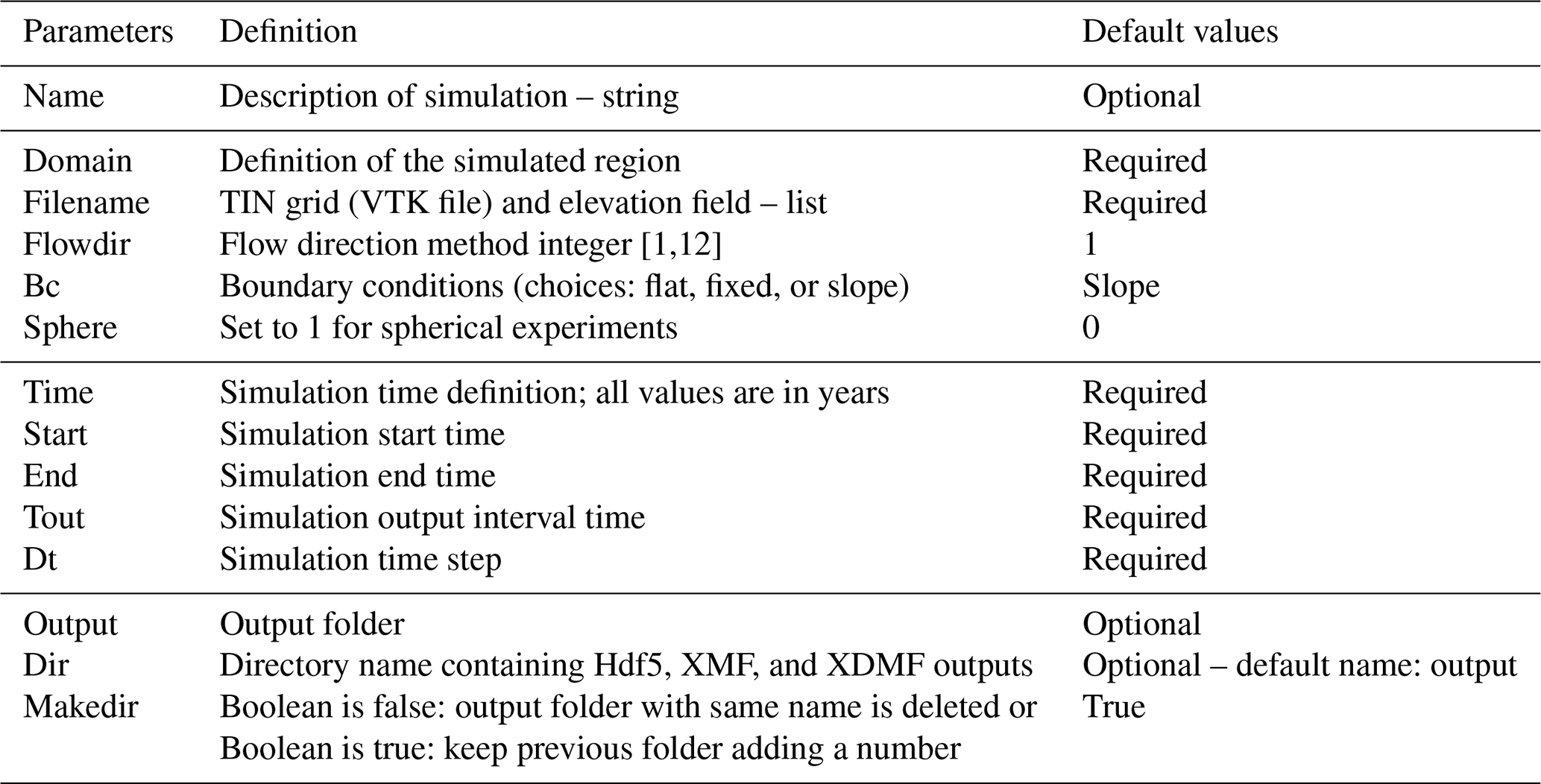
Table 1Input parameters relative to initial surface, temporal extent, and output.
In addition to hillslope processes, a second type of diffusion is available in eSCAPE and consists of distributing freshly deposited marine sediments in deeper regions. This process is the only one treated explicitly, and in this case the length of the diffusion time step Δtm must be less than a Courant–Friedrichs–Lewy (CFL) factor to ensure numerical stability:
where Dm is the diffusion coefficient for the newly deposited marine sediments. Even with a reasonably small time step, Eq. (14) can produce incorrect results. Following Bovy et al. (2016), the following set of inequalities is also added:
where is the flux of sediment from the marine top layer leaving node i towards the downstream neighbours j, hi is the depth of the marine top layer, ηm is the elevation associated with the highest downslope neighbour of i, and α is a factor lower than 1. These inequalities are always satisfied if positive outgoing fluxes are scaled by a factor β given by
In eSCAPE, the marine diffusion of freshly deposited sediment is performed explicitly using the CFL condition described in Eq. (14) and the restriction proposed in Eq. (16).
In this section, I present the main files used to run eSCAPE and to visualise the generated outputs. I then illustrate the capability of the code using a series of three examples presenting two generic models and one global-scale experiment.
3.1 Input parameters and visualisation
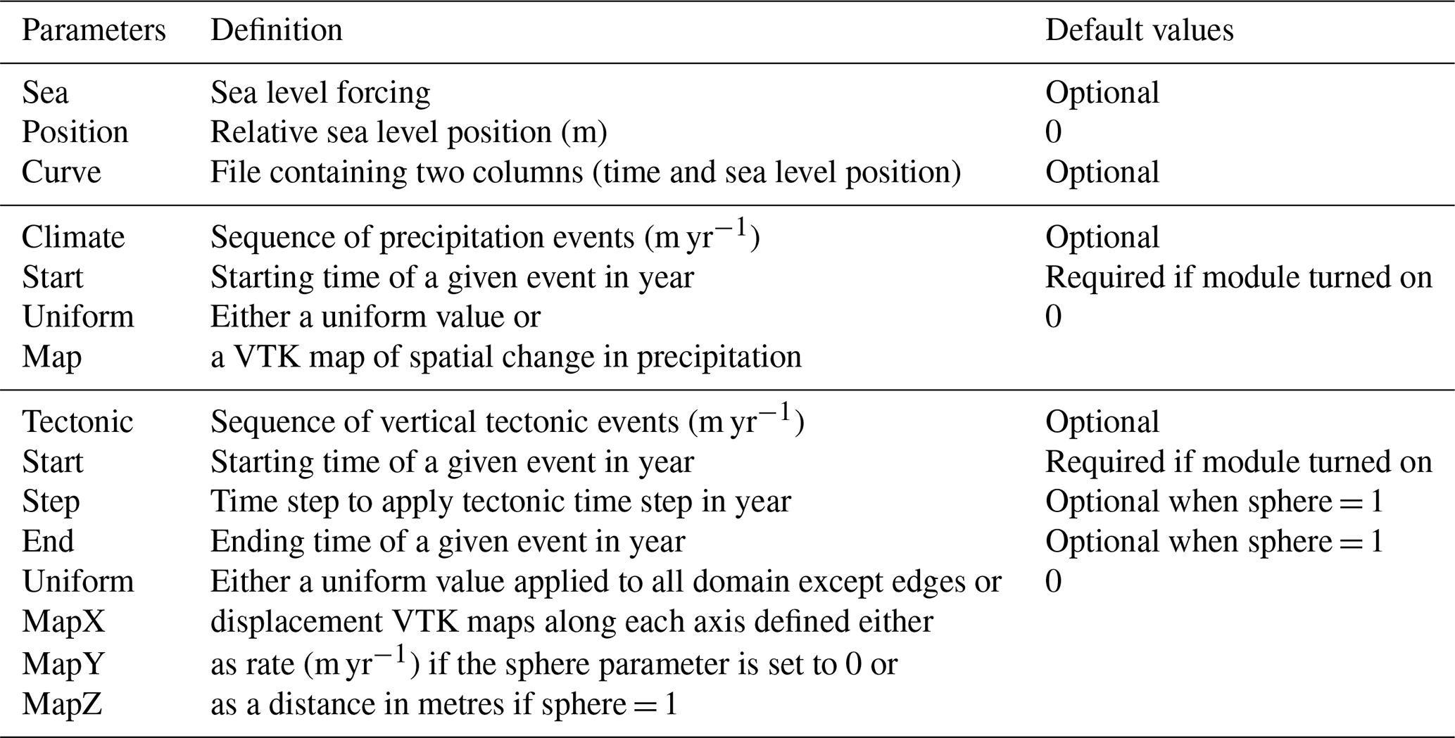
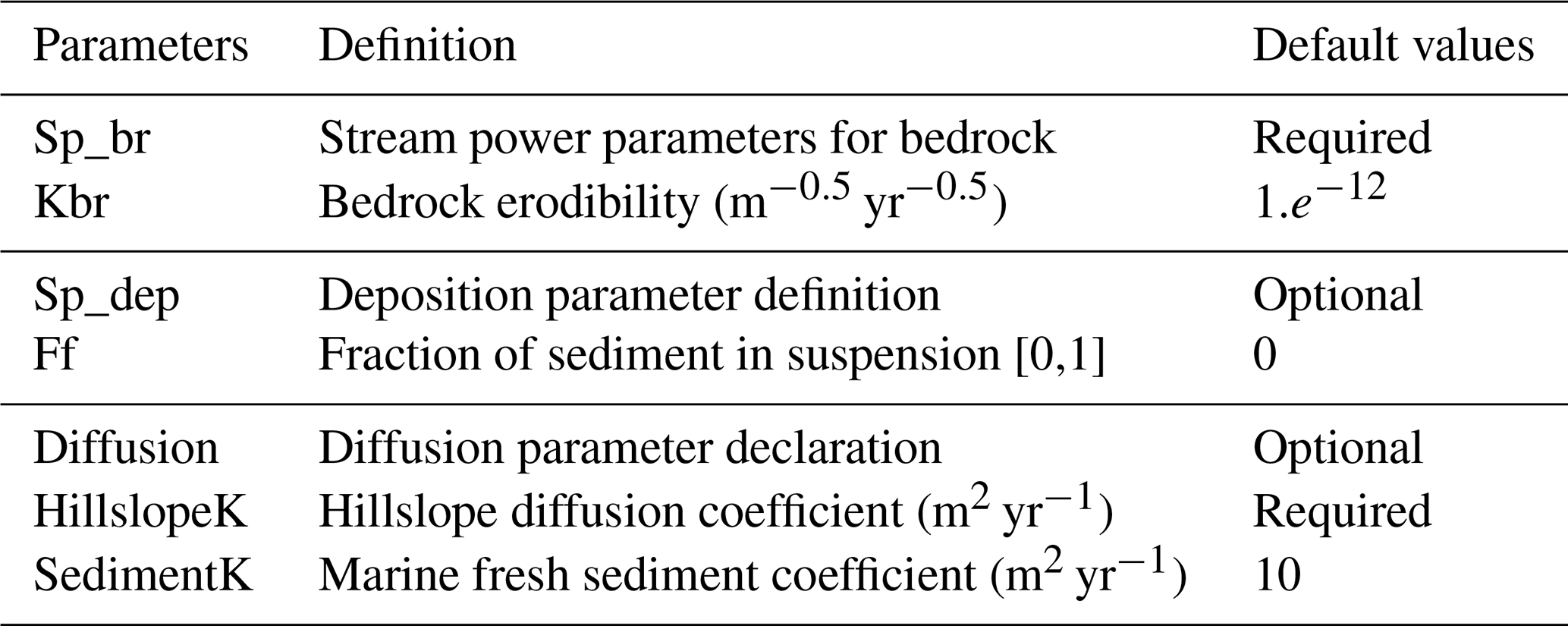
The eSCAPE model uses YAML syntax for its input file. YAML structure is done through indentation (one or more spaces) and sequence items are denoted by a dash. When parsing the input file, the code searches for some specific keywords defined in Tables 1, 2, and 3. Some parameters are optional and only need to be set when specific forces (Table 2) or physical processes (Table 3) are applied to a particular experiment.
All the input parameters that are defined in external files, like the initial surface, different precipitation, or displacement maps, are read from VTK files. These input files are defined on an irregular triangular grid (TIN). Examples of how to produce these files are provided in the eSCAPE demo repository on GitHub and Docker (https://github.com/Geodels/eSCAPE-demo, last access: 23 September 2019). The only exception is the sea level file, which is a two-column CSV file containing in the first column the time in years ordered in ascending order and in the second one the relative position of the sea level in metres (curve in Table 2).
The domain and time keywords (Table 1) are required for any simulation. The flow direction method to be applied in a given simulation is specified with flowdir and takes an integer value ranging between 1 (for SFD) and 12 (for MFD ∕ D∞). On the edges of the domain three types of boundary conditions (bc) are available and applied to all edges: flat, fixed, or slope. The flat option assumes that all edge elevations are set to the elevations of their closest non-edge vertices; the fixed option is used when edge elevations need to remain at their initial positions during the model run, and the slope option defines a slope based on the closest non-edge node average slope.
The climate and tectonic keywords (Table 2) may be defined as a sequence of multiple forcing conditions each requiring a starting time (start in years) and either a constant value applied to the entire grid (uniform) or spatially varying values specified in a file (map).
Surface process parameters (Table 3) define the coefficients for the stream power law (Kbr is K in Eq. 5). It is worth noting that the coefficients m and n are fixed in this version of eSCAPE and take values of 0.5 and 1, respectively. The diffusion keyword defines both hillslope (creep law – Eq. 12; hillslopeK is D in ) and marine diffusion coefficients. The freshly deposited marine sediments are transported based on a diffusion coefficient sedimentK equivalent to Dm in and used in Eq. (13) with the restriction proposed in Eq. (16).
The model outputs are located in the output folder (dir keyword – Table 1) and consist of a time series file named eSCAPE.xdmf and two additional folders (h5 and XMF). The HDF5 files are written individually for each processor and the XMF files combine them together to show the global outputs. The XDMF file is the main entry point for visualising the outputs and should be sufficient for most users. The file can be opened with the ParaView software (Ahrens et al., 2014).
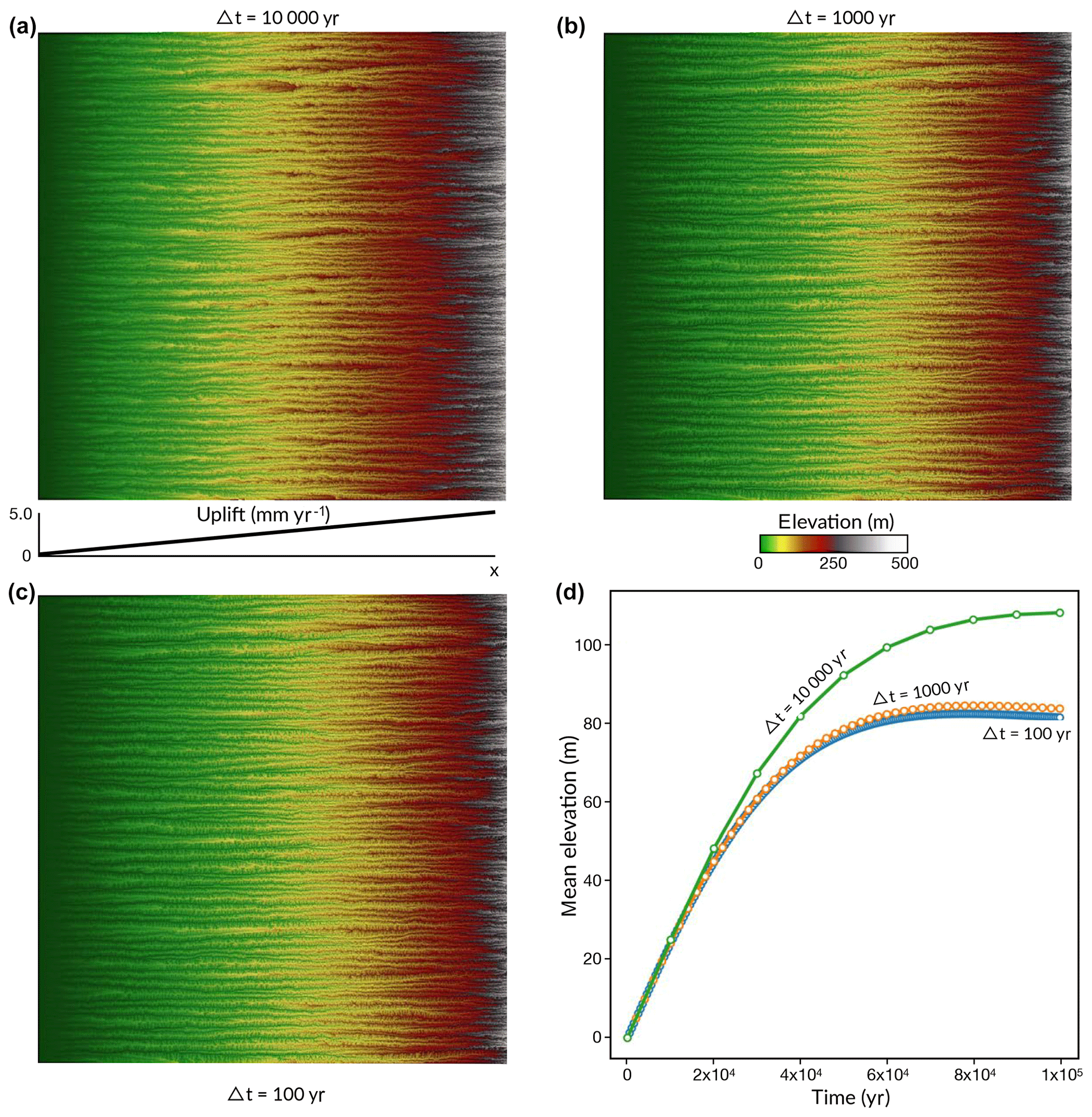
Figure 3Resulting topographies of an initial flat squared surface (100 km side) after 100 000 years of uniform precipitation and linear uplift from west to east. Three simulations are performed in which the time step Δt is set to (a) 104, (b) 103, and (c) 102 years. Panel (d) presents the temporal change in mean elevation for the three cases. Differences between the runs are related to the transient nature of landscape evolution.
3.2 Examples
3.2.1 Analysing the influence of time step on eSCAPE runs
The first example illustrates the effect of increasing time step length on the resulting landscape evolution. The initial surface consists of a flat triangulated squared grid with 100 km sides and approximately 100 m resolution containing ≃ 1.3 million points. This surface is exposed to a uniform precipitation regime of 1 m yr−1 and is uplifted linearly from its fixed western side to the eastern one that experiences an uplift of 5 mm yr−1 (Fig. 3a). The proposed setting is similar to the one in Braun and Willett (2013), and the value of the bedrock erodibility parameter K is set to in order to reach steady state during the simulated 105 years. Under such conditions, the model is purely erosional and therefore neither the aerial and marine sedimentation nor the depression-filling algorithm is considered. In addition, hillslope processes are also turned off, meaning that this example only relies on the implicit parallel flow discharge and erosion equations defined in Sect. 2.1 and 2.2.
Three cases are presented after 105 years for different time steps Δt varying from 104 to 103 and 102 years in Fig. 3a–c, respectively, implying that the number of steps is 10, 100, and 1000. In both cases the implicit schemas converge for the chosen solver and preconditioner (i.e. Richardson with block Jacobian). The solutions for the mean landscape elevation (Fig. 3d) show that the landscape reaches steady state in all cases, and overall the final elevations are in good agreement with a maximum elevation of 482±3 m and a number of catchments nc almost identical between models (). Yet as the time step increases the differences between models increase over time. By the end of the simulation, the mean elevation difference between the case with Δt equals 102 years and the one at 103 years is around 2.5 %, whereas the difference with a Δt of 104 years is above 30 % (Fig. 3d). It illustrates the transient nature of the landscape and its strong dependence on antecedent morphologies. Even small changes in elevation could potentially trigger completely different landscape features. Compared to the explicit algorithm proposed for the drainage area computation in Braun and Willett (2013), the approach here relies on an implicit schema and produces a more stable solution for longer timescales. Yet time step limitations are still required to ensure a good representation of landscape features (e.g. knickpoint propagation) and care should be taken when choosing a given simulation time step.
As mentioned in Sect. 2.1, the iterative linear solvers of the implicit methods for both flow accumulation and erosion use previous time step solution as an initial guess. In cases in which the landscape does not change significantly between consecutive time steps, both the flow accumulation and erosion rates are likely to remain almost unchanged and the number of iterations required by the solver to reach convergence will be small. As an example, if the drainage network remains the same between two iterations, the flow accumulation solver solution will be obtained immediately and the results given directly. It highlights a second implication of the choice of time step. Not only does the time step influence the final landscape morphology, but it also controls the model running time. In some cases, similar running times will be achieved with smaller time steps if solver solutions are obtained in a reduced number of iterations.
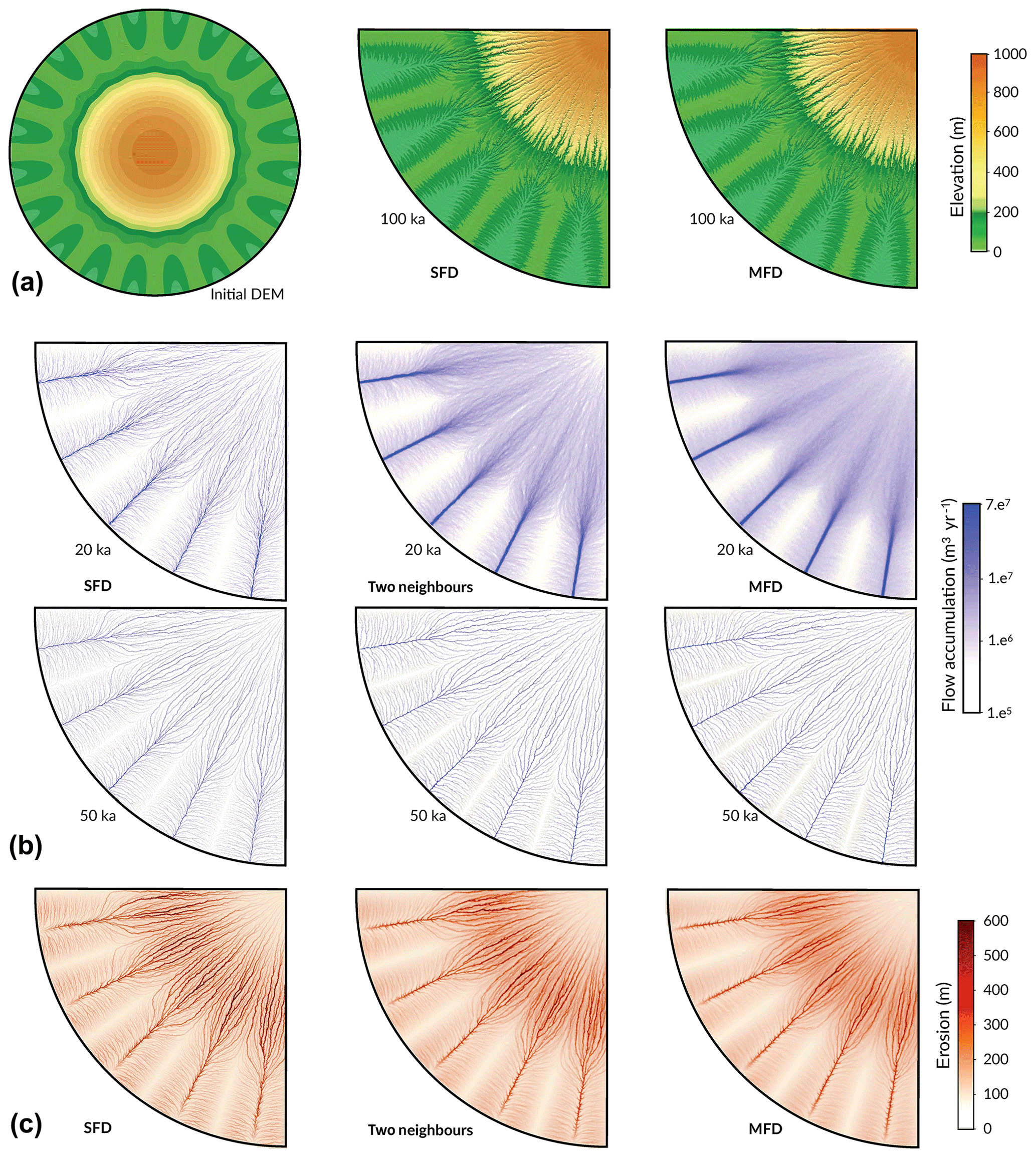
Figure 4Effect of flow-routing algorithms on flow accumulation patterns and associated erosion. Panel (a) presents the initial radially symmetric surface defined with a central high region and a series of distal low-lying valleys. Resulting topographies of the south-west area after 100 000 years of evolution under uniform precipitation for the SFD and MFD algorithms are shown on the right-hand side. Patterns of flow accumulation after 20 000 and 50 000 years for the SFD, two-neighbour, and MFD approaches are presented in panel (b), and estimated landscape erosion at the end of the simulation time interval is given in panel (c).
3.2.2 Comparison of single and multiple flow direction algorithms
In this second example, I present a series of three experiments in which the flow-routing calculations are based on one (SFD), two, and multiple (MFD) flow direction approaches (Fig. 4). In eSCAPE, it is possible to use different flow-routing algorithms by specifying the number of directions (Fig. 1a and flowdir parameter in Table 1) appropriately weighted by the slope that rivers could potentially take when moving downhill.
For this example, the initial surface consists of a rotationally symmetric surface (Fig. 4a) composed of valleys and ridges with the lowest regions (at 0 m of elevation) located on the edges of the domain and increasing to 1000 m towards the centre. The triangulated circular grid of 50 km radius is built with a resolution of approximately 200 m. The three experiments with varying water-routing directions are run for 100 000 years with a Δt of 1000 years under a 1 m yr−1 uniform precipitation. In addition to stream incision (bedrock erodibility K set to ), hillslope processes are also accounted for using a diffusion coefficient D of 10−2 m2 yr−1.
After 20 000 years, the dendritic flow accumulation pattern observed on the surface for the SFD case (Fig. 4b) is analogue to many natural forms of drainage systems but is actually a numerical artefact and depends on the random locations of the nodes in the surface triangulation. By increasing the number of possible downstream directions, this sensitivity to the mesh discretisation is significantly reduced (as illustrated in Fig. 4b, where a second direction is added). In addition, routing flow to more than one destination node allows for a better representation of channel pathway divergence into multiple branches over flat regions (Tucker and Hancock, 2010).
Landscape evolution models tend to be highly dependent on grid resolution, and this dependency is mostly related to the approach used to route water down the surface (Schoorl et al., 2000; Pelletier, 2004; Armitage, 2019). As discussed by Armitage (2019), enabling the node-to-node MFD algorithm decreases the dependence of landscape features (e.g. valley spacing, branching of stream network, sediment flux) on grid resolution. As shown in Fig. 4b and c, the SFD algorithm leads to increased branching of valleys, whereas the MFD approach, by promoting wider flow distribution, produces smoother topography on which local carving of the landscape is reduced. Armitage (2019) also showed that when using models that operate at a scale larger than river-width resolution, the node-to-node MFD algorithm creates landscape features that are not resolution dependent and that evolve closer to the ones observed in nature. Therefore, it is recommended to use more than one downhill direction (flowdir) in eSCAPE when looking at global- and continental-scale landscape evolution or for cases in which multiple resolutions are considered within a given mesh.
3.2.3 Global-scale simulation
The last example showcases a global-scale experiment with eSCAPE. The simulation looks at the evolution of the Earth 200 000 years into the future starting with present-day elevation and precipitation maps. The model is run forward in time without changing the initial forcing conditions, is primarily used to highlight the capabilities of eSCAPE, and does not represent any particular geological situation.
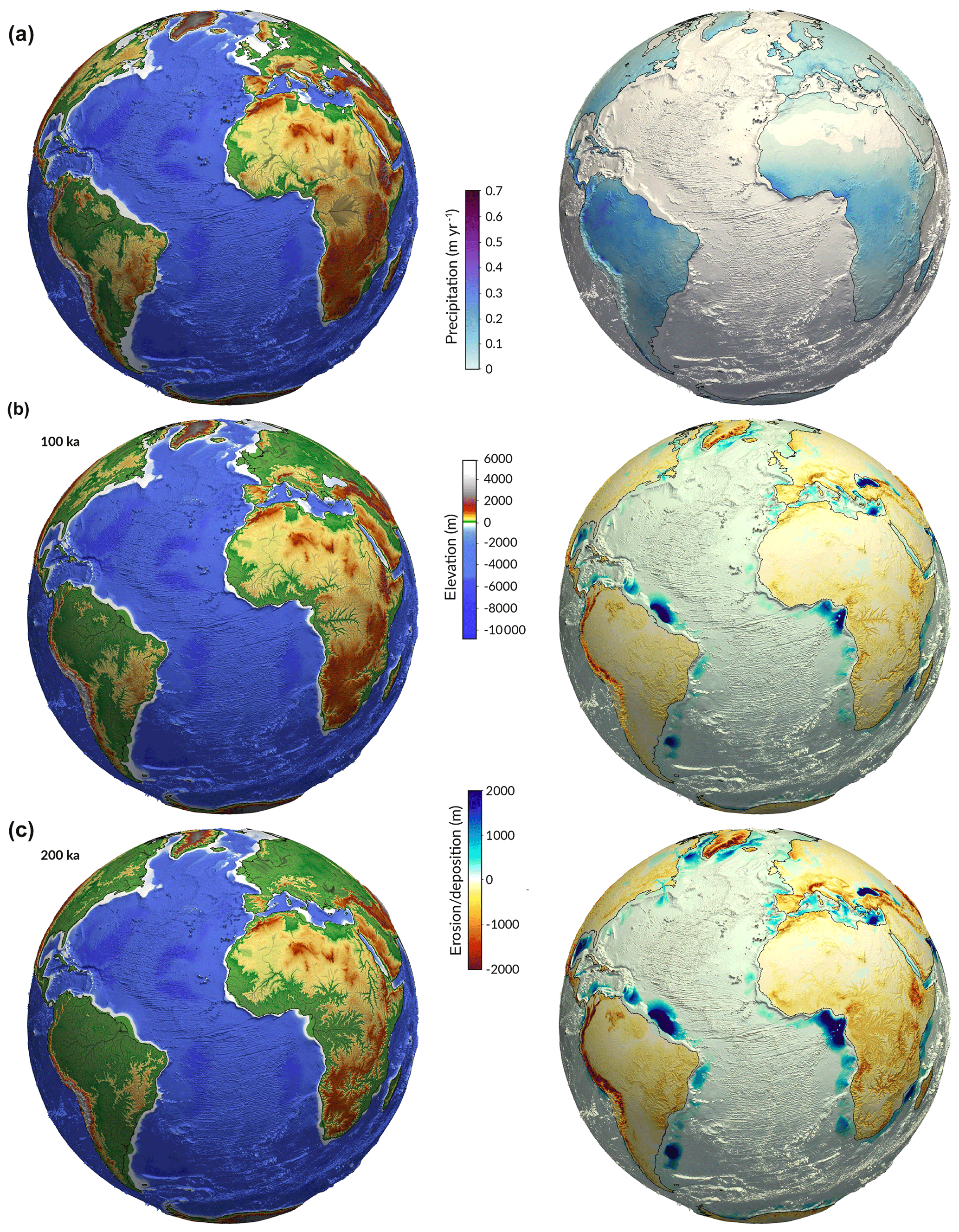
Figure 5The eSCAPE global-scale experiment of Earth's morphological evolution over 200 000 years. Panel (a) presents the initial elevation based on the ETOPO1 dataset and forcing precipitation obtained from the WorldClim dataset. Panels (b) and (c) show the elevation and cumulative erosion–deposition resulting from the action of rivers and hillslope processes at different time intervals.

Figure 6Similar to Fig. 5 from a different perspective.
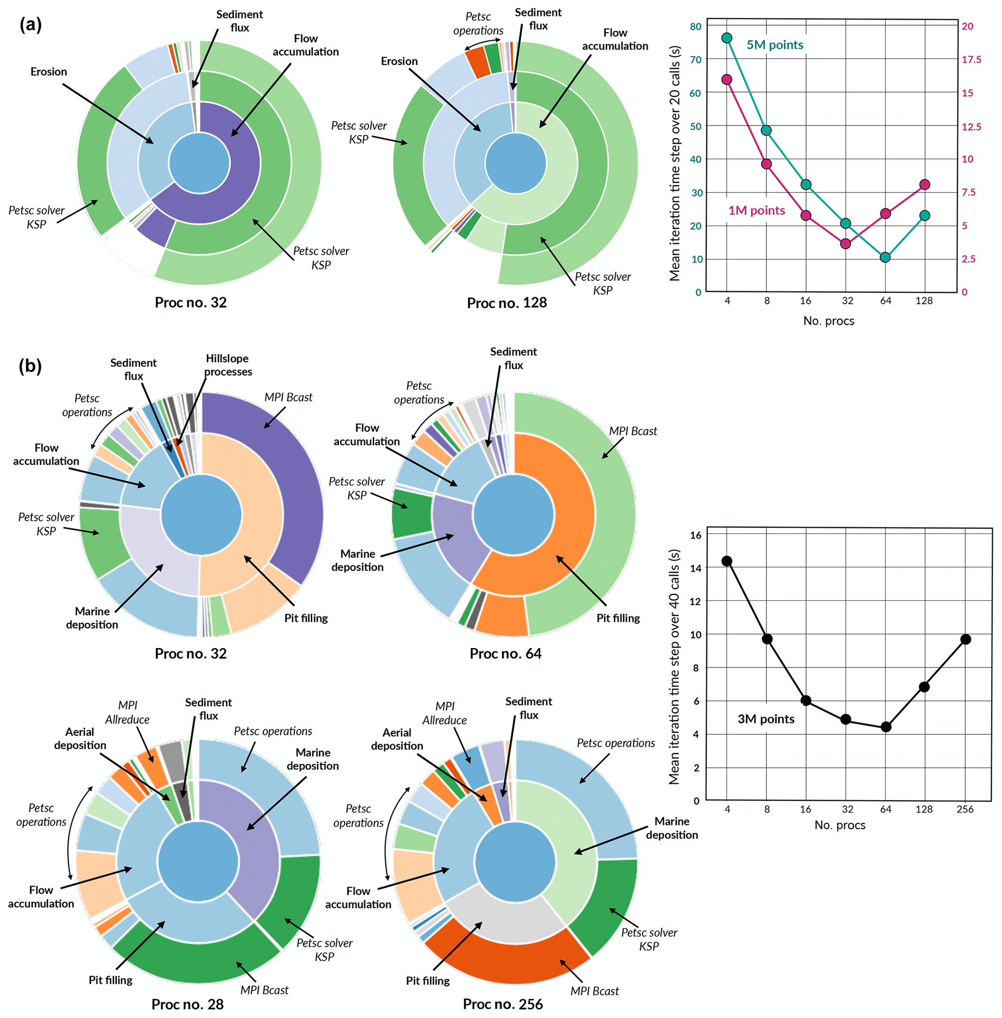
Figure 7Sunburst visualisation obtained from the SnakeViz package showing the profiling results of multiple eSCAPE experiments. The analysis is performed for different numbers of processors (up to 256). On the left-hand side, the fraction of time spent in each function is represented by the angular extent of the different arcs. On the right-hand side the results of the computational runtime versus processor number over a series of time steps are given for experiments of different size. Panel (a) presents the results for purely erosional simulations such as the ones presented in the first example (Sect. 3.2.1). For panel (b) eSCAPE is run with all the processes turned on and uses a global-scale experiment similar to the last example (Sect. 3.2.3).
The elevation is obtained from the ETOPO1 1 arcmin global relief model of the Earth's surface that integrates land topography and ocean bathymetry (Amante and Eakins, 2009). For the rainfall, I summed all the WorldClim gridded climate monthly datasets to obtain a global yearly rainfall map with a spatial resolution of about 1 km2 (Fick and Hijmans, 2017). From these datasets, I then built the initial surface and climate meshes at 16 km resolution consisting of approximately 3 millions points (Figs. 5a and 6a). The model inputs are temporally uniform, but any other climatic scenarios or tectonic conditions could have been chosen for illustration (both vertical: uplift and subsidence; horizontal: advection displacements).
In addition to these grids, the following parameters are chosen: flowdir is set to 5 (similar to the MFD flow-routing approach), the time step Δt equals 500 years, bedrock erodibility K is , the diffusion coefficient D equals 10−1, the fraction of sediment in suspension Ff is 0.3 (Ff parameter in Sect. 2.2 and defined in Table 3), and the marine fresh sediment diffusion Dm is set to 5×10⁵ (see Sect. 2.5 and sedimentK parameter in Table 3). The simulation took 2 h to run on a cluster using 32 processors.
From this set of input parameters, eSCAPE can predict the global evolution of topography (Figs. 5 and 6) and quantify the associated volume and spatial distribution of sediments trapped in continental plains or transported into the marine realm. By recording eroded sediment transport over each drainage basin, eSCAPE provides an estimation of sedimentary mass fluxes carried by major rivers into the ocean (Sect. 2.2). As shown in Figs. 5 and 6, the predicted locations of the largest basin outlets match quite well with observations, and many of the biggest simulated deltaic systems are related to sediment transported by some of the world's largest rivers (Milliman and Syvitski, 1992; Syvitski et al., 2003; Li et al., 2009). The model can also be used to evaluate the evolution of drainage systems, the stability of continental flow directions, the exhumation history of major mountain ranges, the timing and geometry of sedimentary body formation (e.g. deltas or intra-continental deposits), and basin stratigraphy. All these predictions can be directly compared to sedimentary (sediment budgets, paleogeographic maps) or thermochronology data.
This simulation illustrates a global-scale model of Earth's surface evolution. In cases in which paleoclimatic conditions are known, eSCAPE can in principle be used to perform a quantitative analysis of different tectonic forcings with complex spatial and temporal variations. The results of these tests can then be compared with available geological records (such as denudation rates, paleotopographies, and basin sedimentary thicknesses and volumes). In addition to climate and tectonic conditions, it is also possible to impose varying sea level fluctuations over geological times.
As such and even with the limited number of simulated processes, eSCAPE can be used to retrieved global sedimentary basin formation and evolution based on temporal and spatial responses of both landscape and sediment fluxes to different sea level conditions and tectonic and precipitation regimes.
The performance of the implicit flow accumulation, erosion, and sediment transport algorithms is strongly dependent on the choice of solver and preconditioner. As shown in Sect. 2.1 and 2.2, the forms of the matrices are not symmetric or positive, and in this case only a limited number of iterative solvers and preconditioners is suitable. From the extensive analysis provided in Richardson et al. (2014), the non-Krylov solver based on the Richardson method (Richardson, 1910) has been chosen in eSCAPE as it converged with the greatest number of preconditioners and exhibited superior scaling. For the preconditioner, several candidates (SOR, ILU, ASM) are available (Saad, 2003) and I decided to use the block Jacobian preconditioner as it is one of the simplest methods and produces in combination with the Richardson solver good scalability (Richardson et al., 2014). Yet other combinations such as the Richardson solver with the Euclid preconditioner (i.e. HYPRE package; Falgout et al., 2012) might exhibit better scalability in some cases.
The analysis of the profiling work realised in Fig. 7a suggests that for purely erosive models (similar to the ones presented in Sect. 3.2.1) most of the computational time is spent solving the Richardson iterative method (PETSc solver KSP). From the graph on the right-hand side of Fig. 7a, one can deduce that performance improvements are obtained when the problem size increases. However, the scaling performance decreases when reaching 32–64 processors depending on the problem size. This does not agree with some of the conclusions from Richardson et al. (2014), wherein the scaling of the implicit drainage accumulation algorithm continues even for large numbers of processors (> 192). To improve performance, I will be exploring two directions. First, the problem might be related to the chosen solver and preconditioner combination, and I will run new tests using the HYPRE package as discussed above. Secondly, the poor performance for larger processors might also be linked to issues related to either the Python PETSc wrapper or installation problems and incompatibilities between some of the compilers and packages that I used. In the future, different software libraries and compiler versions from GNU and Intel will be tested and might help to improve the performance for an increasing number of processors.
For experiments accounting for marine deposition and pit filling, a similar trend is found when comparing performance against processor number (right-hand side of Fig. 7b). However, the results from the profiling (left-hand side of Fig. 7b) suggest that more than half of the computation time is now spent on non-PETSc work with the biggest proportion related to the pit-filling function. In eSCAPE, the priority-flood algorithm is performed in serial (see Sect. 2.3). This is the major limitation of the code as shown by the time spent in broadcasting the information from the master node to the other processors (MPI Bcast in Fig. 7b). To take advantage of parallel architectures, several authors (Wallis et al., 2009; Tesfa et al., 2011; Yıldırım et al., 2015; Zhou et al., 2017) have proposed partitioning the implementation of depression-filling algorithms. However, most of these methods require frequent interprocess communication and synchronisation. This becomes even more problematic in the case of eSCAPE, wherein the depression-filling algorithm needs to be performed at every time step (Barnes, 2019). Barnes (2017) presented an alternative to the aforementioned parallelisation methods that limits the number of communications. Yet this approach is not fully satisfactory as it only fills the depressions up to the spilling elevation but does not provide a way of efficiently implementing the ϵ variant of the algorithm proposed in Barnes et al. (2014). Finding a strategy to perform a parallel version of the ϵ variant of the priority-flood algorithm or to efficiently fill the depressions (Cordonnier et al., 2019) while providing flow directions on flat surface will likely greatly improve the performance of eSCAPE.
In this paper, I describe eSCAPE, an open-source, Python-based software designed to simulate sediment transport, landscape dynamics, and sedimentary basin evolution under the influence of climate, sea level, and tectonics. In its current form, eSCAPE relies on the stream power and creep laws to simulate the physical processes acting on the Earth's surface. The main difference with other landscape evolution models relies on the formulation used to solve the system of equations. The approach builds upon the implicit drainage area calculation from Richardson et al. (2014) and consists of a series of implicit iterative algorithms for calculating multiple flow direction and erosion deposition written in matrix form. As a result, the obtained systems can be solved with widely available parallel linear solver packages such as PETSc.
Performance analysis shows good parallel scaling for a small number of processors (under 64 processors as shown in Sect. 4) but some work is required for larger numbers. The code profiling suggests that the main issue is in the interprocess communications happening when broadcasting the pit-filling information computed in serial by the master to the other processors. In the future, a parallel approach allowing for depression-filling and flow direction computation over flat regions will be critical to improve the overall performance of the code.
Examples are provided in the paper and available through the Docker container. They illustrate the extent of temporal and spatial scales that can be addressed using eSCAPE. As such, this code is highly versatile and useful for geological applications related to source to sink problems at a regional, continental, and, for the first time, global scale. It is already possible to use eSCAPE to simulate the global geological evolution of the Earth's landscape at about 1 km resolution, providing accurate estimates of quantities such as large-scale erosion rates, sediment yields, and sedimentary basin formation. In the future, the code will be coupled with atmospheric and geodynamic models to bridge the gap between local- and global-scale predictions of Earth's past and future evolutions.
The source code with examples (Jupyter Notebooks) is archived as a release version v2.0 from Zenodo (https://doi.org/10.5281/zenodo.3239569; Salles, 2019). The code is licenced under the GNU General Public License v3.0. The easiest way to use eSCAPE is via our Docker container (https://hub.docker.com/u/geodels/, last access: 23 September 2019; search for “Geodels escape-docker” on Kitematic), which is shipped with the complete list of dependencies and the case studies presented in this paper.
The author declares that there is no conflict of interest.
The author acknowledges the Sydney Informatics Hub and the University of Sydney's high-performance computing cluster Artemis for providing the high-performance computing resources that have contributed to the research results reported within this paper. The author also acknowledges the technical assistance of David Kohn from the Sydney Informatics Hub, which was supported by project no. 3789, and from the Artemis HPC Grand Challenge. I also thank John Armitage, Benoit Bovy, and the journal editor for their comments that greatly improved the paper.
This paper was edited by Thomas Poulet and reviewed by Benoit Bovy and John Armitage.
Ahrens, J., Jourdain, S., O'Leary, P., Patchett, J., Rogers, D. H., and Petersen, M.: An image-based approach to extreme scale in situ visualization and analysis, Proceedings of the International Conference for High Performance Computing, https://doi.org/10.1109/SC.2014.40, 2014. a
Amante, C. and Eakins, B. W.: ETOPO1 1 Arc-Minute Global Relief Model: Procedures, Data Sources and Analysis., NOAA Technical Memorandum NESDIS NGDC-24, 19 pp., available at: http://www.ngdc.noaa.gov/mgg/global/global.html (last access: 23 September 2019), 2009. a
Armitage, J. J.: Short communication: flow as distributed lines within the landscape, Earth Surf. Dynam., 7, 67–75, https://doi.org/10.5194/esurf-7-67-2019, 2019. a, b, c, d
Balay, S., Brown, J., Buschelman, K., Gropp, W. D., Kaushik, D., Knepley, M. G., McInnes, L. C., Smith, B. F., and Zhang, H.: Argonne National Laboratory, PETSc, available at: http://www.mcs.anl.gov/petsc (last access: 23 September 2019), 2012. a, b, c
Barnes, R.: Parallel non-divergent flow accumulation for trillion cell digital elevation models on desktops or clusters, Environ. Model. Softw., 92, 202–212, https://doi.org/10.1016/j.envsoft.2017.02.022, 2017. a, b
Barnes, R.: Accelerating a fluvial incision and landscape evolution model with parallelism, Geomorphology, 330, 28–39, https://doi.org/10.1016/j.geomorph.2019.01.002, 2019. a, b, c
Barnes, R., Lehman, C., and Mulla, D.: Priority-flood: An optimal depression-filling and watershed-labeling algorithm for digital elevation models, Comput. Geosci., 62, 117–127, https://doi.org/10.1016/j.cageo.2013.04.024, 2014. a, b, c, d, e, f
Beaumont, C., Fullsack, P., and Hamilton, J.: Erosional control of active compressional orogens, in: Thrust Tectonics, edited by: McClay, K. R., Chapman Hall, New York, 1–18, https://doi.org/10.1007/978-94-011-3066-0_1, 1992. a, b
Bellugi, D., Dietrich, W. E., Stock, J., McKean, J., Kazian, B., and Hargrove, P.: Spatially explicit shallow landslide susceptibility mapping over large areas, in: Fifth International Conference on Debris-flow Hazards Mitigation, Mechanics, Prediction and Assessment, edited by: Genevois, R., Hamilton, D. L., and Prestininzi, A., Casa Editrice Universita La Sapienza, Rome, pp. 309–407, https://doi.org/10.4408/IJEGE.2011-03.B-045, 2011. a
Beucher, R., Moresi, L., Giordani, J., Mansour, J., Sandiford, D., Farrington, R., Mondy, L., Mallard, C., Rey, P., Duclaux, G., Kaluza, O., Laik, A., and Moroon, S.: UWGeodynamics: A teaching and research tool for numerical geodynamic modelling, J. Open Source Softw., 4, 1136, https://doi.org/10.21105/joss.01136, 2019. a
Bianchi, V., Salles, T., Ghinassi, M., Billi, P., Dallanave, E., and Duclaux, G.: Numerical modeling of tectonically driven river dynamics and deposition in an upland incised valley, Geomorphology, 241, 353–370, https://doi.org/10.1016/j.geomorph.2015.04.007, 2015. a
Bovy, B., Braun, J., and Demoulin, A.: Soil production and hillslope transport in mid-latitudes during the last glacial-interglacial cycle: a combined data and modelling approach in northern Ardennes, Earth Surf. Proc. Land., 41, 1758–1775, https://doi.org/10.1002/esp.3993, 2016. a, b
Braun, J. and Sambridge, M.: Modelling landscape evolution on geological time scales: a new method based on irregular spatial discretization, Basin Research, 9, 27–52, 1997. a, b
Braun, J. and Willett, S. D.: A very efficient O(n), implicit and parallel method to solve the stream power equation governing fluvial incision and landscape evolution, Geomorphology, 180–181, 170–179, 2013. a, b, c
Carretier, S., Martinod, P., Reich, M., and Godderis, Y.: Modelling sediment clasts transport during landscape evolution, Earth Surf. Dynam., 4, 237–251, https://doi.org/10.5194/esurf-4-237-2016, 2016. a
Chen, A., Darbon, J., and Morel, J.-M.: Landscape evolution models: a review of their fundamental equations, Geomorphology, 219, 68–86, 2014. a
Cordonnier, G., Bovy, B., and Braun, J.: A versatile, linear complexity algorithm for flow routing in topographies with depressions, Earth Surf. Dynam., 7, 549–562, https://doi.org/10.5194/esurf-7-549-2019, 2019. a, b
Coulthard, T. J., Macklin, M. G., and Kirkby, M. J.: A cellular model of Holocene upland river basin and alluvial fan evolution, Earth Surf. Proc. Land., 27, 269–288, https://doi.org/10.1002/esp.318, 2002. a, b
Culling, W. E. H.: Soil creep and the development of hillside slopes, J. Geology, 71, 127–161, 1963. a, b
Davy, P. and Lague, D.: Fluvial erosion/transport equation of landscape evolution models revisited., J. Geophys. Res.-Earth, 114, F03007, https://doi.org/10.1029/2008JF001146, 2009. a, b
DiBiase, R. A., Whipple, K. X., Heimsath, A. M., and Ouimet, W. B.: Landscape form and millennial erosion rates in the San Gabriel Mountains, CA, Earth Planet. Sc. Lett., 289, 134–144, 2010. a
Dietrich, W. E., Bellugi, D., Sklar, L. S., Stock, J., Heimsath, A. M., and Roering, J. J.: Geomorphic transport laws for predicting landscape form and dynamics, in: Prediction in Geomorphology, edited by: Wilcock, P. R. and Iverson, R. M., 135, 103–132, Blackwell Publishing Ltd, 2003. a
Eddins, S.: Upslope area – Forming and solving the flow matrix, MathWorks, available at: http://blogs.mathworks.com/steve/2007/08/07/upslope-area-flow-matrix (last access: 23 September 2019), 2007. a
Falgout, R., Kolev, T., Schroder, J., Vassilevski, P., and Yang, U. M.: Lawrence Livermore National Laboratory, HYPRE Package, available at: https://computation.llnl.gov/casc/hypre/software.html (last access: 23 September 2019), 2012. a
Fernandes, N. and Dietrich, W. E.: Hillslope evolution by diffusive processes: The timescale for equilibrium adjustments, Water Resour. Res., 33, 1307–1318, 1997. a, b
Fick, S. E. and Hijmans, R. J.: WorldClim 2: new 1-km spatial resolution climate surfaces for global land areas, Int. J. Climatol., 37, 4302–4315, https://doi.org/10.1002/joc.5086, 2017. a
Foufoula-Georgiou, E., Ganti, V., and Dietrich, W. E.: A nonlocal theory of sediment transport on hillslopes, J. Geophys. Res.-Earth, 115, F00A16, https://doi.org/10.1029/2009JF001280, 2010. a
Grieve, S., Mudd, S., and Hurst, M.: How long is a hillslope?, Earth Surf. Process. Landforms, 41, 1039–1054, https://doi.org/10.1002/esp.3884, 2016a. a
Grieve, S. W. D., Mudd, S. M., Hurst, M. D., and Milodowski, D. T.: A nondimensional framework for exploring the relief structure of landscapes, Earth Surf. Dynam., 4, 309–325, https://doi.org/10.5194/esurf-4-309-2016, 2016b. a
Hobley, D. E. J., Sinclar, H. D., Mudd, S. M., and Cowie, P. A.: Field calibration of sediment flux dependent river incision, J. Geophys. Res.-Earth, 116, F04017, https://doi.org/10.1029/2010JF001935, 2011. a
Hobley, D. E. J., Adams, J. M., Nudurupati, S. S., Hutton, E. W. H., Gasparini, N. M., Istanbulluoglu, E., and Tucker, G. E.: Creative computing with Landlab: an open-source toolkit for building, coupling, and exploring two-dimensional numerical models of Earth-surface dynamics, Earth Surf. Dynam., 5, 21–46, https://doi.org/10.5194/esurf-5-21-2017, 2017. a, b, c
Hodge, R. A. and Hoey, T. B.: Upscaling from grain-scale processes to alluviation in bedrock channels using a cellular automaton model, J. Geophys. Res., 117, F01017, https://doi.org/10.1029/2011JF002145, 2012. a
Howard, A. D., Dietrich, W. E., and Seidl, M. A.: Modeling fluvial erosion on regional to continental scales, J. Geophys. Res.-Sol. Ea., 99, 13971–13986, 1994. a, b, c, d
Jenson, S. and Domingue, J.: Extracting topographic structure from digital elevation data for geographic information system analysis, Photogramm. Eng. Remote Sens., 54, 1593–1600, 1988. a
Jones, E., Oliphant, T., and Peterson, P.: SciPy: Open source scientific tools for Python, available at: http://www.scipy.org/ (last access: 23 September 2019), 2001. a, b
Lague, D.: Reduction of long-term bedrock incision efficiency by short-term alluvial cover intermittency, J. Geophys. Res., 115, F02011, https://doi.org/10.1029/2008JF001210, 2010. a
Larsen, I. J. and Montgomery, D. R.: Landslide erosion coupled to tectonics and river incision, Nat. Geosci., 5, 468–473, 2012. a
Li, F., Griffiths, C. M., Dyt, C. P., Weill, P., Feng, M., Salles, T., and Jenkins, C.: Multigrain seabed sediment transport modelling for the south-west Australian Shelf, Mar. Freshwater Res. 60, 774–785, https://doi.org/10.1071/MF08049, 2009. a
Mark, D. M.: Network models in geomorphology, Modelling Geomorphological Systems, edited by: Anderson, M. G., Wiley, NY, 73–97, 1988. a
Milliman, J. and Syvitski, J.: Geomorphic/tectonic control of sediment discharge to the ocean: the importance of small mountainous rivers, J. Geol., 100, 525–544, 1992. a
Murphy, B. P., Johnson, J. P. L., Gasparini, N. M., and Sklar, L. S.: Chemical weathering as a mechanism for the climatic control of bedrock river incision, Nature, 532, 223–227, 2016. a
O'Callaghan, J. F. and Mark, D. M.: The extraction of drainage networks from digital elevation data, Comput. Vision Graph., 28, 323–344, 1984. a
Pelletier, J. D.: Persistent drainage migration in a numerical landscape evolution model, Geophys. Res. Lett., 31, L20501, https://doi.org/10.1029/2004GL020802, 2004. a
Perron, J. T. and Hamon, J. L.: Equilibrium form of horizontally retreating, soil-mantled hillslopes: Model development and application to a groundwater sapping landscape, J. Geophys. Res., 117, F01027, https://doi.org/10.1029/2011JF002139, 2012. a, b
Planchon, O. and Darboux, F.: A fast, simple and versatile algorithm to fill the depressions of digital elevation models, Catena, 46, 159–176, https://doi.org/10.1016/S0341-8162(01)00164-3, 2002. a
Quinn, P., Beven, K., Chevallier, P., and Planchon, O.: The prediction of hillslope flow paths for distributed hydrological modelling using digital terrain models, Hydrol. Process., 5, 59–79, https://doi.org/10.1002/hyp.3360050106, 1991. a
Richardson, A., Hill, C. N., and Perron, J. T.: IDA: An implicit, parallelizable method for calculating drainage area, Water Resour. Res., 50, 4110–4130, https://doi.org/10.1002/2013WR014326, 2014. a, b, c, d, e, f, g, h, i
Richardson, L.: On the approximate arithmetical solution by finite differences of physical problems involving differential equations, with an application to the stresses in a masonry dam, Proc. R. Soc. London Ser. A, 83, 335–336, 1910. a, b
Roering, J. J., Kirchner, J. W., Sklar, L. S., and Dietrich, W. E.: Hillslope evolution by nonlinear creep and landsliding: An experimental study, Geology, 29, 143–146, 1999. a, b, c
Roering, J. J., Kirchner, J. W., and Dietrich, W. E.: Hillslope evolution by nonlinear, slope-dependent transport: Steady state morphology and equilibrium adjustment timescales, J. Geophys. Res.-Sol. Ea., 106, 16499–16513, 2001. a, b
Saad, Y.: Iterative Methods for Sparse Linear Systems, Society for Industrial and Applied Mathematics, Philadelphia, PA, 2003. a
Salles, T.: Badlands: A parallel basin and landscape dynamics model, SoftwareX, 5, 195–202, 2016. a
Salles, T.: eSCAPE: parallel global-scale landscape evolution model, J. Open Source Softw., 3, 964, https://doi.org/10.21105/joss.00964, 2018. a, b
Salles, T.: Geodels/eSCAPE: eSCAPE: Regional to Global Scale Landscape Evolution Model v2.0 (Version v2.0), Zenodo, https://doi.org/10.5281/zenodo.3239569 , 2019. a
Salles, T. and Duclaux, G.: Combined hillslope diffusion and sediment transport simulation applied to landscape dynamics modelling., Earth Surf. Process Landf., 40, 823–839, 2015. a
Salles, T. and Hardiman, L.: Badlands: An open-source, flexible and parallel framework to study landscape dynamics, Comput. Geosci., 91, 77–89, 2016. a, b
Salles, T., Griffiths, C., Dyt, C., and Li, F.: Australian shelf sediment transport responses to climate change-driven ocean perturbations, Mar. Geol., 282, 268–274, 2011. a
Salles, T., Flament, N., and Müller, D.: Influence of mantle flow on the drainage of eastern Australia since the Jurassic Period, Geochem. Geophy. Geosy., 18, 280–305, 2017. a, b
Salles, T., Ding, X., and Brocard, G.: pyBadlands: A framework to simulate sediment transport, landscape dynamics and basin stratigraphic evolution through space and time, PLOS ONE, 13, 1–24, https://doi.org/10.1371/journal.pone.0195557, 2018. a, b
Schoorl, J. M., Sonneveld, M. P. W., and Veldkamp, A.: Three-dimensional landscape process modelling: the effect of DEM resolution, Earth Surf. Proc. Land., 25, 1025–1034, 2000. a
Schwanghart, W. and Kuhn, N. J.: Topotoolbox: A set of Matlab functions for topographic analysis, Environ. Modell. Softw., 25, 770–781, https://doi.org/10.1016/j.envsoft.2009.12.002, 2010. a
Shobe, C. M., Tucker, G. E., and Barnhart, K. R.: The SPACE 1.0 model: a Landlab component for 2-D calculation of sediment transport, bedrock erosion, and landscape evolution, Geosci. Model Dev., 10, 4577–4604, https://doi.org/10.5194/gmd-10-4577-2017, 2017. a, b, c
Simoes, M., Braun, J., and Bonnet, S.: Continental-scale erosion and transport laws: A new approach to quantitatively investigate macroscale landscapes and associated sediment fluxes over the geological past, Geochem. Geophy. Geosy., 11, Q09001, https://doi.org/10.1029/2010GC003121, 2010. a
Simpson, G. and Schlunegger, F.: Topographic evolution and morphology of surfaces evolving in response to coupled fluvial and hillslope sediment transport, J. Geophys. Res., 108, 2300, https://doi.org/10.1029/2002JB002162, 2003. a
Snyder, N. P., Whipple, K. X., Tucker, G. E., and Merritts, D. J.: Importance of a stochastic distribution of floods and erosion thresholds in the bedrock river incision problem, Water Resour. Res., 108, 2117, https://doi.org/10.1029/2001JB001655, 2003. a
Syvitski, J., Peckham, S., Hilberman, R., and T., M.: Predicting the terrestrial flux of sediment to the global ocean: a planetary perspective, Sediment. Geol., 162, 5–24, https://doi.org/10.1016/S0037-0738(03)00232-X, 2003. a
Tarboton, D. G.: A new method for the determination of flow directions and upslope areas in grid digital elevation models, Water Resour. Res., 33, 309–319, https://doi.org/10.1029/96WR03137, 1997. a
Tarboton, D. G.: Utah State University, TauDEM Web page, available at: http://hydrology.usu.edu/taudem/taudem5 (last access: 23 September 2019), 2013. a
Tesfa, T., Tarboton, D., Watson, D., Schreuders, K., Baker, M., and Wallace, R.: Extraction of hydrological proximity measures from DEMs using parallel processing, Environ. Model. Softw., 26, 1696–1709, 2011. a
Thieulot, C., Steer, P., and Huismans, R. S.: Three-dimensional numerical simulations of crustal systems undergoing orogeny and subjected to surface processes, Geochem. Geophy. Geosy., 15, 4936–4957, 2014. a
Tomkin, J. H., Brandon, M. T., Pazzaglia, F. J., Barbour, J. R., and Willett, S. D.: Quantitative testing of bedrock incision models for the Clearwater River, NW Washington State, J. Geophys. Res., 108, 2308, https://doi.org/10.1029/2001JB000862, 2003. a
Tucker, G. E. and Bradley, D. N.: Trouble with diffusion: Reassessing hillslope erosion laws with a particle-based model, J. Geophys. Res.-Earth, 115, F00A10, https://doi.org/10.1029/2009JF001264, 2010. a
Tucker, G. E. and Bras, R. L.: Hillslope processes, drainage density, and landscape morphology, Water Resour. Res., 34, 2751–2764, 1998. a
Tucker, G. E. and Hancock, G. R.: Modelling landscape evolution, Earth Surf. Proc. Land., 35, 28–50, 2010. a, b, c, d, e, f
Tucker, G. E. and Slingerland, R.: Drainage basin responses to climate change, Water Resour. Res., 33, 2031–2047, 1997. a, b, c
Tucker, G. E. and Slingerland, R. L.: Erosional dynamics, flexural isostasy, and long-lived escarpments: A numerical modeling study, J. Geophys. Res., 99, 12229–12243, https://doi.org/10.1029/94JB00320, 2017. a
Tucker, G. E., Lancaster, S. T., Gasparini, N. M., Bras, R. L., and Rybarczyk, S. M.: An object-oriented framework for distributed hydrologic and geomorphic modeling using triangulated irregular networks, Comput. Geosci., 27, 959–973, 2001. a
Turowski, J. M. and Hodge, R.: A probabilistic framework for the cover effect in bedrock erosion, Earth Surf. Dynam., 5, 311–330, https://doi.org/10.5194/esurf-5-311-2017, 2017. a
Valla, P. G., van der Beek, P. A., and Lague, D.: Fluvial incision into bedrock: insights from morphometric analysis and numerical modeling of gorges incising glacial hanging valleys (Western Alps, France), J. Geophys. Res.-Earth, 115, F02010, https://doi.org/10.1029/2008JF001079, 2010. a
van der Beek, P. and Bishop, P.: Cenozoic river profile development in the Upper Lachlan catchment (SE Australia) as a test of quantitative fluvial incision models, J. Geophys. Res., 108, 2309, https://doi.org/10.1029/2002JB002125, 2003. a
Wallace, R. M., Tarboton, D. G., Watson, D. W., Schreuders, K. A. T., and Tesfa, T. K.: Parallel algorithms for processing hydrologic properties from digital terrain, in: Sixth International Conference on Geographic Information Science, edited by: Purves, R. and Weibel, R., Zurich, Switzerland, 2010. a
Wallis, C., Wallace, R. M., Tarboton, D. G., Watson, D. W., Schreuders, K. A. T., and Tesfa, T. K.: Hydrologic terrain processing using parallel computing, in: 18th World IMACS Congress and MODSIM09 International Congress on Modelling and Simulation, edited by: Anderssen, R. S., Braddock, R. D., and Newham, L. T. H., 2540–2545, 2009. a, b
Wang, L. and Liu, H.: An efficient method for identifying and filling surface depressions in digital elevation models for hydrologic analysis and modelling, Int. J. Geogr. Inf. Sci., 20, 193–213, https://doi.org/10.1080/13658810500433453, 2006. a
Wei, H., Zhou, G., and Fu, S.: Efficient Priority-Flood depression filling in raster digital elevation models, Int. J. Digit Earth, 12, 415–427, https://doi.org/10.1080/17538947.2018.1429503, 2018. a
Willgoose, G. R., Bras, R. L., and Rodriguez-Iturbe, I.: A physically based coupled network growth and hillslope evolution model: 1 – Theory, Water Resour. Res., 27, 1671–1684, https://doi.org/10.1029/91WR00935, 1991. a, b
Yang, R., Willett, S. D., and Goren, L.: In situ low-relief landscape formation as a result of river network disruption, Nature, 526–529, https://doi.org/10.1038/nature14354, 2015. a
Yıldırım, A., Watson, D., Tarboton, D., and Wallace, R.: A virtual tile approach to raster-based calculations of large digital elevation models in a shared-memory system, Comput. Geosci., 82, 78–88, 2015. a
Zhou, G., Sun, Z., and Fu, S.: An efficient variant of the priority-flood algorithm for filling depressions in raster digital elevation models, Comput. Geosci., 90, 87–96, https://doi.org/10.1016/j.cageo.2016.02.021, 2016. a
Zhou, G., Liu, X., Fu, S., and Sun, Z.: Parallel Identification and Filling of Depressions in Raster Digital Elevation Models, Int. J. Geogr. Inf. Sci., 31, 1061–1078, https://doi.org/10.1080/13658816.2016.1262954, 2017. a, b