TheDiaTo (v1.0) – a new diagnostic tool for water, energy and entropy budgets in climate models

This work presents the Thermodynamic Diagnostic Tool (TheDiaTo), a novel diagnostic tool for investigating the thermodynamics of climate systems with a wide range of applications, from sensitivity studies to model tuning. It includes a number of modules for assessing the internal energy budget, the hydrological cycle, the Lorenz energy cycle and the material entropy production. The routine takes as inputs energy fluxes at the surface and at the top of the atmosphere (TOA), which allows for the computation of energy budgets at the TOA, the surface and in the atmosphere as a residual. Meridional enthalpy transports are also computed from the divergence of the zonal mean energy budget from which the location and intensity of the maxima in each hemisphere are calculated. Rainfall, snowfall and latent heat fluxes are received as inputs for computation of the water mass and latent energy budgets. If a land–sea mask is provided, the required quantities are separately computed over continents and oceans. The diagnostic tool also computes the annual Lorenz energy cycle (LEC) and its storage and conversion terms by hemisphere and as a global mean. This is computed from three-dimensional daily fields of horizontal wind velocity and temperature in the troposphere. Two methods have been implemented for the computation of the material entropy production: one relying on the convergence of radiative heat fluxes in the atmosphere (indirect method) and the other combining the irreversible processes occurring in the climate system, particularly heat fluxes in the boundary layer, the hydrological cycle and the kinetic energy dissipation as retrieved from the residuals of the LEC (direct method). A version of these diagnostics has been developed as part of the Earth System Model eValuation Tool (ESMValTool) v2.0a1 in order to assess the performances of CMIP6 model simulations, and it will be available in the next release. The aim of this software is to provide a comprehensive picture of the thermodynamics of the climate system, as reproduced in the state-of-the-art coupled general circulation models. This can prove useful for better understanding anthropogenic and natural climate change, paleoclimatic climate variability, and climatic tipping points.

1 Introduction

The climate can be viewed as a forced, dissipative non-equilibrium system exchanging energy with the external environment. The inhomogeneous absorption of solar radiation is an ongoing source of available potential energy. The complex mixture of fluids is then set into motion by the conversion of available potential into mechanical energy via a vast range of nonlinear processes. The kinetic energy is eventually dissipated through viscous stress and converted back into heat. Such processes can be described by taking advantage of the theory of the non-equilibrium thermodynamics of continuous multiphase media and, in particular, of fluids. The presence of (possibly fluctuating) fluxes of matter, chemical species and energy is a key characteristic of a non-equilibrium system. The steady state is reached as a result of a potentially complex balance of positive and negative feedbacks and through the interplay of processes with very diverse timescales and physical underpinning mechanisms. The climate is a prime example of this, with observed variability extending over many orders of magnitude in terms of both spatial and temporal scales and with many extremely complex subdomains – the atmosphere, the ocean, the cryosphere, the biosphere, the active soil – which themselves have very diverse characteristic internal timescales and are nonlinearly coupled (Peixoto and Oort, 1992; Lucarini et al., 2014).

It is a major endeavour of contemporary science to improve our understanding of the climate system in the context of the past, present and projected future conditions. This is key for understanding, as far as the past goes, the co-evolution of life and of the physicochemical properties of the ocean, soil and atmosphere, as well as for addressing the major challenge faced by our planet as a result of the current anthropogenic climate change. Improving climate models is key to nearing these goals, and, indeed, efforts aimed in this direction have been widely documented (see the related chapter on the last report of the Intergovernmental Panel on Climate Change, 2013). Intercomparing and validating climate models is far from being a trivial task, also at a purely conceptual level (Lucarini, 2013; Frigg et al., 2015). Difficulties can only increase when looking at the practical side: how should meaningful metrics to study the performance of climate models be chosen? Should they be motivated in terms of basic processes of the climate system or in terms of relevance for an end user of climate services? In order to put some order in this conundrum, the community of climate modellers has developed a set of standardized metrics for intercomparing and validating climate models (Eyring et al., 2016a). For obvious reasons, the choice made for such metrics has been biased – for possibly good reasons – in the direction of providing ready-to-use information for end users. What we propose in this paper is a novel software containing process-based and end-user-relevant diagnostics that is capable of providing an integrated perspective on the problem of model validation and intercomparison. The goal here is to examine models through the lens of their dynamics and thermodynamics in the view of the ideas enunciated above about complex non-equilibrium systems reaching a steady state as a result of an interplay of multiscale processes. The metrics that we propose here are based on the analysis of energy and water budgets and transports, of energy transformations, and of entropy production. We summarize below some of the key concepts behind our work.

1.1 Energy

In order to be in steady state, a non-equilibrium system in contact with an external environment must have a vanishing – on average – energy budget. Inconsistencies in the overall energy budget of long-term stationary simulations have been carefully pointed out (Lucarini and Ragone, 2011; Mauritsen et al., 2012), and various aspects of the radiative and heat transfers within the atmosphere and between the atmosphere and the oceans have been evaluated in order to constrain models to a realistic climate (Wild et al., 2013; Loeb et al., 2015). A substantial bias in the energy budget of the atmosphere, in particular, has been identified in many global climate models (GCMs), resulting from either the imperfect closure of the kinetic energy budget (Lucarini and Ragone, 2011) or of the mass balance in the hydrological cycle (Liepert and Previdi, 2012). This picture is made even more complicated by the difficult task of having an accurate observational benchmark of the Earth's energy budget (e.g. Loeb et al., 2009; von Schuckmann et al., 2016). Many authors have recently suggested that the improvement of climate models requires improving the energetic consistency of the modelled system (Hansen et al., 2011; Lucarini et al., 2011, 2014). Rather than a proxy for a changing climate, surface temperatures and precipitation changes can be better viewed as a consequence of a non-equilibrium steady-state system which is responding to a radiative energy imbalance through complex interacting feedbacks. A changing climate, under the effect of an external transient forcing, can only be properly addressed if the energy imbalance, and the way it is transported within the system and converted into different forms, is taken into account. The skill of the models at representing historical energy and heat exchanges in the climate system has been assessed by comparing numerical simulations against available observations, where available (Allan et al., 2014; Smith et al., 2015), including the fundamental problem of ocean heat uptake (Exarchou et al., 2015).

A key element in defining the steady state of the climate system is the balance between the convergence of the horizontal (mostly meridional) enthalpy fluxes by the atmospheric and the oceanic circulations and the radiative imbalance at the top of the atmosphere (TOA). The net radiative imbalance is positive (in-bound) in the low latitudes and negative in the high latitudes, and a compensating horizontal transport must be present in order to ensure steady state. This transport dramatically reduces the meridional temperature gradient with respect to what would be set by radiative–convective equilibrium (Manabe and Wetherald, 1967), i.e. in the absence of large-scale atmospheric and oceanic transport. Differences in the boundary conditions, in the forcing and dissipative processes, and in chemical and physical properties of the atmosphere and ocean lead to a specific partitioning of the enthalpy transport between the two geophysical fluids; a different partitioning associated with the same total transport would lead to significantly different climate conditions (Rose and Ferreira, 2013; Knietzsch et al., 2015). The role of meridional heat transports in different paleoclimate scenarios and in relation to different forcing has been addressed in various studies (see e.g. Caballero and Langen, 2005; Fischer and Jungclaus, 2010). The question of whether the current state-of-the-art climate models are able to correctly represent the global picture as well as the details of the atmospheric and oceanic heat transports has been analysed with mixed findings (Lucarini et al., 2011, 2014; Lembo et al., 2016).

In order to understand how heat is transported by the geophysical fluids, one should clarify what sets them into motion. We focus here on the atmosphere. A comprehensive view of the energetics fuelling the general circulation is given by the Lorenz energy cycle (LEC) framework (Lorenz, 1955; Ulbrich and Speth, 1991). This provides a picture of the various processes responsible for the conversion of available potential energy (APE) – the excess of potential energy with respect to a state of thermodynamic equilibrium (see Tailleux, 2013, for a review) – into kinetic energy and dissipative heating. Under stationary conditions, the dissipative heating exactly equals the mechanical work performed by the atmosphere. Thus, the LEC formulation allows us to constrain the atmosphere to the first law of thermodynamics, and the system as a whole can be interpreted as a heat engine under dissipative non-equilibrium conditions (Ambaum, 2010). The strength of the LEC, or in other words the rate of the conversion of available potential energy (APE) into kinetic energy (KE), has been evaluated in observational-based datasets (Li et al., 2007; Pan et al., 2017) and climate models (Lucarini et al., 2010a; Marques et al., 2011), with estimates generally ranging from 1.5 to 3.5 W m⁻². A considerable source of uncertainty is the hydrostatic assumption, on which the LEC formulation relies, which can lead to significant underestimation of the kinetic energy dissipation (Pauluis and Dias, 2012). The usual formulation of the LEC can be seen as describing energy exchanges and transformation at a coarse-grained level, at which non-hydrostatic processes are not relevant and the system is accurately described by primitive equations. An efficiency can also be attributed to the atmosphere as a heat engine, assuming the system is analogous to an engine operating between a warmer and a colder temperature (Lucarini, 2009). This approach has been generalized by Pauluis (2011) in order to account for the role of water vapour.

1.2 Water

Water is an essential ingredient of the climate system, and the hydrological cycle plays an important role in the energy pathways of the climate system. Water vapour and clouds influence the radiative processes inside the system, and water phase exchanges are extremely energy intensive. As in the case of energy imbalances, a closed water-mass-conserving reproduction of the hydrological cycle is essential, not only because of the diverse implications of the hydrological cycle for energy balance and transports in the atmosphere, but also because of its sensitivity to climate change (Held and Soden, 2006) and the importance of the cloud and water vapour feedbacks (Hartmann, 1994). The energy budget is influenced by semi-empirical formulations of the water vapour spectrum (Wild et al., 2006), and, similarly, the energy budget influences the moisture budget by means of uncertainties in aerosol–cloud interactions and mechanisms of tropical deep convection (Wild and Liepert, 2010; Liepert and Previdi, 2012). Water mass budget has been assessed in observations (L'Ecuyer et al., 2015; Rodell et al., 2015), as well as in climate models, focusing on the hydrological cycle alone (Terai et al., 2018) or evaluating it in conjunction with the energy budgets (Demory et al., 2014; Vannière et al., 2019). Therefore, a global-scale evaluation of the hydrological cycle, both from a moisture and from an energetic perspective, is considered an integral part of overall diagnostics for the thermodynamics of climate system.

1.3 Entropy

The climate system has long been recognized as featuring irreversible processes through dissipation and mixing in various forms, leading to the production of entropy (Paltridge, 1975), which is a key characteristic of non-equilibrium systems (Prigogine, 1962). Several early attempts (Peixoto and Oort, 1992; Johnson, 1997; Goody, 2000) were made to understand the complex nature of irreversible climatic processes. Recent works (Bannon, 2015; Bannon and Lee, 2017) have proposed an innovative approach by partitioning the system into a control volume made of matter and radiation, which exchanges energy with its surroundings (building on Goody, 2000, early works). Raymond (2013) has described the entropy budget of an aggregated dry air + water vapour parcel. From a macroscopic point of view, “material entropy production” generally refers to the entropy produced by the geophysical fluids in the climate system, which is not related to the properties of the radiative fields but rather to the irreversible processes related to the motion of these fluids. Material entropy production is dominated by phase changes and water vapour diffusion, as outlined by Pauluis and Held (2002). Lucarini (2009) underlined the link between entropy production and efficiency of the climate engine, which were then applied to study climatic tipping points, in particular the snowball–warm Earth critical transition (Lucarini et al., 2010b). This allowed for the definition of a wider class of climate response metrics (Lucarini et al., 2010a) that have been used to study planetary circulation regimes (Boschi et al., 2013). A constraint has also been proposed to the entropy production of the atmospheric heat engine, given by the emerging importance of non-viscous processes in a warming climate (Laliberté et al., 2015).

Given the multiscale properties of the climate system, accurate energy and entropy budgets are affected by subgrid-scale parametrizations (see also Kleidon and Lorenz, 2004; Kunz et al., 2008). These and the discretization of the numerical scheme are generally problematic in terms of conservation principles (Gassmann and Herzog, 2015) and can eventually lead to macroscopic model drifts (Mauritsen et al., 2012; Gupta et al., 2013; Hobbs et al., 2016; Hourdin et al., 2017). See Lucarini and Fraedrich (2009) for a theoretical analysis in a simplified setting.

1.4 This paper

We present TheDiaTo v1.0, a new software for diagnosing the mentioned aspects of the thermodynamics of climate systems (i.e. the energy and water mass budgets and meridional transports, the LEC strength, and the material entropy production) in a broad range of global-scale gridded datasets of the atmosphere. The diagnostic tool provides global metrics, allowing for straightforward comparison of different products. These include the following:

• top-of-atmosphere, atmospheric and surface energy budgets;

• total, atmospheric and oceanic meridional enthalpy transports;

• water mass and latent energy budget;

• strength of the LEC by means of kinetic energy dissipation conversion terms; and

• material entropy production by both direct and indirect methods.

The software is structured in terms of independent modules so that users can subset the metrics according to their interest. A version of the tool has been developed as part of the ESMValTool community effort (Eyring et al., 2016b) to provide a standardized set of diagnostics for the evaluation of Coupled Model Intercomparison Project Phase 6 (CMIP6) multi-model ensemble simulations (Eyring et al., 2016a). The current version at the time of writing was ESMValTool v2.0a1, and a new version is soon to be released including TheDiaTo v1.0.

Therefore, our goal is to equip climate modellers and developers with tools for better understanding the strong and weak points of the models of interest. The aim is to reduce the risk of a model having accurate reproductions of quantities of common interest, such as surface temperature or precipitation, but for the wrong dynamical reasons. This is a necessary first step in the direction of creating a suite of model diagnostics composed of process-oriented metrics.

The paper is structured as follows. The dataset requirements are described in Sect. 2. We then establish the methods used in each module (Sect. 3). In Sect. 4 an example is given of application to a 20-year-long model run. In Sect. 5 the evolution of the metrics under three different scenarios in the CMIP5 multi-model ensemble (Taylor et al., 2012) is evaluated. A summary and conclusions are given in Sect. 6.

2 Data and software requirements

The diagnostic tool consists of a set of independent modules, each, except the first one, being triggered by a switch decided by the user: energy budgets and enthalpy transports, hydrological cycle, Lorenz energy cycle, and material entropy production via the direct or indirect method.

The software ingests all variables as fields on a regular longitude–latitude grid covering the whole globe. Therefore, the tool is suitable for the evaluation of any kind of gridded dataset, provided that it contains the necessary variables on a regular grid, including blends of observations and reanalyses. In our description of the software features, we focus on model evaluation and multi-model intercomparison.

For the LEC computation, 3-D fields are required, stored in pressure levels at a daily or finer temporal resolution. If the model does not store data where the surface pressure is lower than the respective pressure levels, daily mean or higher-resolution data of near-surface temperatures and horizontal velocity fields are also required for vertical interpolation. For all other computations, 2-D fields are required as monthly means at TOA and at the surface. Input variables are given as separate files in NetCDF format. For model intercomparisons (Sect. 5), computations are performed on the native grid of the model. Variables are identified according to their variable names. Those are required to comply with the Climate and Forecast (CF; http://cfconventions.org/Data/cf-documents/overview/article.pdf, last access: 26 August 2019) and Climate Model Output Rewriter (CMOR; http://pcmdi.github.io/cmor-site/tables.html, last access: 26 August 2019) standards. Datasets that do not comply with the CF–CMOR-compliant names are reformatted through ESMValTool built-in preprocessing routines if recognized (for more detail, refer to the dedicated report on ESMValTool v1.0; Eyring et al., 2016b). An overview of the required variables is provided in Table 1.

Table 1 Variables used in the modules of the diagnostic tool.

¹ Precipitation fluxes are provided (kg m⁻² s⁻¹). The software also accepts other units of measure and related fields, depending on the known formats by the ESMValTool preprocessor. ² Specific humidity can also be given as a near-surface two-dimensional field (when available) or the lowermost pressure level of the three-dimensional specific humidity field (variable name: huss).

Energy budgets are computed from residuals of instantaneous radiative shortwave (SW) and longwave (LW) fluxes at TOA. At the surface, SW and LW fluxes are combined with instantaneous turbulent latent and sensible heat fluxes (see Sect. 3). The radiative fluxes (except the outgoing LW radiation, which is only upwelling) are composed of an upwelling and downwelling component that are as defined positive. The heat fluxes at the surface are computed in climate models from the usual bulk formulas, with different models differing in the choice of the parameters, and are positive upwards. Water mass and latent energy budgets are computed from evaporation (implied from latent heat turbulent fluxes at the surface), rainfall and snowfall instantaneous fluxes. Some models might provide cumulative energy and water mass fields instead of instantaneous fluxes. If this is the case, the ESMValTool preprocessor performs the conversion to instantaneous fluxes, depending on the analysis time step.

For the LEC module, 3-D fields of the three components of velocity and temperatures are needed at the daily resolution. For the 3-D fields, there is no specific constraint on the number of pressure levels, although the programme has been tested on the standard pressure level vertical discretization used in CMIP5 outputs, consisting of 17 levels from 1000 to 1 hPa. The programme then subsets the troposphere between 900 and 100 hPa. LEC computation is performed on Fourier coefficients of the temperature and velocity fields. The 2-D fields of temperature and horizontal velocity are also required in order to fill gaps in the pressure level discretization by interpolating from the surface on a reference vertical profile. As further discussed later (Sect. 5.2), this technique introduces an inevitable source of uncertainty.

If explicitly required by the user, the programme is also able to perform computations of energy budgets, enthalpy transports and the hydrological cycle on oceans and continents separately, provided a land–sea mask is supplied. This can either be in the form of land area fraction or a binary mask.

The ESMValTool architecture is implemented as a Python package, and the latest version is available at https://doi.org/10.17874/ac8548f0315 (last access: 26 August 2019), where the dependencies and installation requirements are also described. If using TheDiaTo v.1 as part of the ESMValTool architecture, the user is asked to specify the path to input data, work and plot directories, as well as some details of the local machine. A dedicated namelist (named as “`recipe”) includes information on the diagnostics, such as a brief description, the reference literature and the developers. The user is asked to specify the name of the dataset to be analysed, which must be recognized by the ESMValTool preprocessor. The diagnostic tool is thus run, calling the ESMValTool interface with the associated recipe.

A stand-alone version of the software is maintained as well, utilizing Python bindings for Climate Data Operators (CDO, 2015). It consists of a Python script, reading a namelist with user settings (such as directory paths, model names and options for the usage of the modules). The stand-alone version is publicly available in a GitHub repository (https://github.com/ValerioLembo/TheDiaTo_v1.0, last access: 26 August 2019), where detailed instructions on the usage of the software are given.

3 Methods

3.1 Energy budgets and meridional enthalpy transports

By making the crucial assumption that the heat content of liquid and solid water in the atmosphere, the heat associated with the phase transitions in the atmosphere, and the effect of salinity and pressure in the oceans are negligible, we can write the total specific energy per unit mass for the subdomains constituting the climate system as ${\mathit{ϵ}}_{\text{a}}={\mathit{u}}^{\mathrm{2}}+c_{v}T+\mathit{\varphi }+Lq$ for the atmosphere, ${\mathit{ϵ}}_{\text{o}}={\mathit{u}}^{\mathrm{2}}+c_{w}T+\mathit{\varphi }$ for the ocean, and ${\mathit{ϵ}}_{\text{s}}=c_{\text{s}}T+\mathit{\varphi }$ for solid earth and ice. Here u is the velocity vector; c_v, c_w and c_s are the specific heat of the atmospheric mix at constant volume, water and the solid medium, respectively, L is the latent heat of vaporization of water, q the specific humidity and ϕ the gravitational potential. This leads to an equation for the evolution of the local specific energy in the atmosphere as such (Peixoto and Oort, 1992):

$$\begin{array}{}\text{(1)}& {\displaystyle \frac{\partial \mathit{\rho }\mathit{ϵ}}{\partial t}}=-\mathrm{\nabla }\cdot \left({\mathbf{J}}_h+\mathbf{R}+{\mathbf{H}}_{\text{S}}+{\mathbf{H}}_{\text{L}}\right)-\mathrm{\nabla }(\mathit{\tau }\cdot \mathit{u}),\end{array}$$

where ${\mathbf{J}}_h=(\mathit{\rho }E+p)\mathit{u}$ is the specific enthalpy transport, R is the net radiative flux, H_L and H_S are the turbulent sensible and latent heat fluxes, respectively, and τ is the stress tensor. By neglecting the kinetic energy component and vertically integrating Eq. (1), we find an equation for the energy tendencies at each latitude (ϕ), longitude (λ) and time for the whole climate system, for the atmosphere, and for the surface below it:

$$\begin{array}{}\text{(2)}& {\displaystyle }\left\{\begin{array}{l}{\dot{E}}_{\text{t}}(\mathit{\lambda },\mathit{\varphi })=S_t^{\downarrow }(\mathit{\lambda },\mathit{\varphi })-S_t^{\uparrow }(\mathit{\lambda },\mathit{\varphi })-L_{\text{t}}(\mathit{\lambda },\mathit{\varphi })-\mathrm{\nabla }\cdot J_t(\mathit{\lambda },\mathit{\varphi })\\ =R_{\text{t}}(\mathit{\lambda },\mathit{\varphi })-\mathrm{\nabla }\cdot J_t(\mathit{\lambda },\mathit{\varphi })\\ {\dot{E}}_{\text{a}}(\mathit{\lambda },\mathit{\varphi })=R_{\text{t}}(\mathit{\lambda },\mathit{\varphi })-F_{\text{s}}(\mathit{\lambda },\mathit{\varphi })-\mathrm{\nabla }\cdot J_a(\mathit{\lambda },\mathit{\varphi })\\ =F_{\text{a}}(\mathit{\lambda },\mathit{\varphi })-\mathrm{\nabla }\cdot J_a(\mathit{\lambda },\mathit{\varphi })\\ {\dot{E}}_{\text{s}}(\mathit{\lambda },\mathit{\varphi })=S_{\text{s}}(\mathit{\lambda },\mathit{\varphi })+L_{\text{s}}(\mathit{\lambda },\mathit{\varphi })-H_S^{\uparrow }(\mathit{\lambda },\mathit{\varphi })-H_{\text{L}}^{\uparrow }(\mathit{\lambda },\mathit{\varphi })\\ -\mathrm{\nabla }\cdot J_o(\mathit{\lambda },\mathit{\varphi })\\ =F_{\text{s}}(\mathit{\lambda },\mathit{\varphi })-\mathrm{\nabla }\cdot J_o(\mathit{\lambda },\mathit{\varphi }),\end{array}\right.\end{array}$$

where ${\dot{E}}_{\text{t}}$, ${\dot{E}}_{\text{a}}$ and ${\dot{E}}_{\text{s}}$ denote the total, atmospheric and surface energy tendencies, respectively. $S_{\text{s}}=S_s^{\uparrow }(\mathit{\lambda },\mathit{\varphi })-S_s^{\uparrow }(\mathit{\lambda },\mathit{\varphi })$ and $L_{\text{s}}=L_s^{\uparrow }(\mathit{\lambda },\mathit{\varphi })-L_s^{\uparrow }(\mathit{\lambda },\mathit{\varphi })$ are the net SW and LW radiative fluxes at the surface, respectively, and $S_t^{\downarrow }$, $S_s^{\downarrow }$, $S_t^{\uparrow }$ and $S_s^{\uparrow }$ the TOA (t) and surface (s) upward (^↑) and downward (^↓) SW radiative fluxes, respectively (and similarly for LW radiative fluxes, denoted by L, provided that there is no downward LW flux at TOA). R_t, F_a and F_s are the total, atmospheric and surface net energy fluxes, respectively. Net fluxes are defined as positive when there is a net energy input and negative when there is a net output. J_t, J_a and J_o are the meridional total, atmospheric and oceanic enthalpy transports. Oceanic transports are assumed to be related to surface energy budgets because the long-term enthalpy transports through land are nearly negligible (Trenberth and Solomon, 1994; Trenberth et al., 2001).

When globally averaged, Eq. (2) can be rewritten as (Lucarini et al., 2014)

$$\begin{array}{}\text{(3)}& {\displaystyle }\left\{\begin{array}{l}{\dot{E}}_{\text{t}}=R_{\text{t}}\\ {\dot{E}}_{\text{a}}=R_{\text{t}}-F_{\text{s}}=F_{\text{a}}\\ {\dot{E}}_{\text{s}}=F_{\text{s}}.\end{array}\right.\end{array}$$

Given the small thermal inertia of the atmosphere compared to the oceans, the TOA energy imbalance is expected to be transferred for the most part to the ocean interior, with F_a much smaller than F_s (Levitus et al., 2012; Loeb et al., 2012; Smith et al., 2015). This is usually not reproduced in climate models (e.g. Lucarini and Ragone, 2011; Loeb et al., 2015; Lembo et al., 2019a).

Under steady-state conditions, the tendency of the internal energy of the system will vanish when averaged over sufficiently long time periods. We can thus zonally average Eq. (2) and derive the long-term time means of the meridional heat transports or, more appropriately in this formulation, “meridional enthalpy transports”:

$$\begin{array}{}\text{(4)}& \left\{\begin{array}{l}{T}_{\text{t}}\left(\mathit{\varphi }\right)=\mathrm{2}\mathit{\pi }{\int }_{\mathit{\varphi }}^{\mathit{\pi }/\mathrm{2}}{a}^{\mathrm{2}}\cos {\mathit{\varphi }}^{\prime }\langle \stackrel{\mathrm{‾}}{R_{\text{t}}\left({\mathit{\varphi }}^{\prime }\right)}\rangle \text{d}{\mathit{\varphi }}^{\prime }\\ T_{\text{a}}\left(\mathit{\varphi }\right)=\mathrm{2}\mathit{\pi }{\int }_{\mathit{\varphi }}^{\mathit{\pi }/\mathrm{2}}{a}^{\mathrm{2}}\cos {\mathit{\varphi }}^{\prime }\langle \stackrel{\mathrm{‾}}{F_{\text{a}}\left({\mathit{\varphi }}^{\prime }\right)}\rangle \text{d}{\mathit{\varphi }}^{\prime }\\ T_{\text{o}}\left(\mathit{\varphi }\right)=\mathrm{2}\mathit{\pi }{\int }_{\mathit{\varphi }}^{\mathit{\pi }/\mathrm{2}}{a}^{\mathrm{2}}\cos {\mathit{\varphi }}^{\prime }\langle \stackrel{\mathrm{‾}}{F_{\text{s}}\left({\mathit{\varphi }}^{\prime }\right)}\rangle \text{d}{\mathit{\varphi }}^{\prime },\end{array}\right.\end{array}$$

where T_t, T_a and T_o denote the steady-state total, atmospheric and oceanic meridional enthalpy transports, a the Earth's radius, 〈 〉 long-term time averaging and overbars the zonal mean quantities. The stationary condition has to be achieved in the models if the system is unforced. If the system is forced, for instance by a transient greenhouse gas forcing, a correction is applied in order to avoid unphysical cross-polar transports. This correction can be applied as long as the weak non-stationarity condition holds (Carissimo et al., 1985); i.e. the latitudinal variability of the net energy flux is much larger than the global mean imbalance (see Lucarini and Ragone, 2011). The energy fluxes are modified as follows:

$$\begin{array}{}\text{(5)}& \langle {\stackrel{\mathrm{‾}}{B}}_x\left(\mathit{\varphi }\right){\rangle }_{\text{co}}=\langle {\stackrel{\mathrm{‾}}{B}}_x\left(\mathit{\varphi }\right)\rangle -\langle {\stackrel{\mathrm{‾}}{B}}_x\left(\mathit{\varphi }\right)\rangle /\mathrm{2}\mathit{\pi }a,\end{array}$$

where B_x refers to R_t, F_a or F_s.

Peak intensities and latitudes are computed as metrics for these transports.

3.2 Hydrological cycle

The atmospheric moisture budget is obtained by globally averaging precipitation and evaporation fluxes. The latter are derived from surface latent heat fluxes as

$$\begin{array}{}\text{(6)}& E={\displaystyle \frac{H_{\text{L}}}{L_{\text{v}}}},\end{array}$$

where E from now on denotes the evaporation fluxes and $L_{\text{v}}=\mathrm{2.5008}\times {\mathrm{10}}^{\mathrm{6}}$ J kg⁻¹ the latent heat of evaporation (assumed to be constant). If H_L is given in units of watts per square metre, the implied evaporation flux is in units of kilometres per square metre per second. Rainfall fluxes are derived from total (P) and snowfall (P_s) precipitation as

$$\begin{array}{}\text{(7)}& P_{\text{r}}=P-P_{\text{s}}.\end{array}$$

Under the stationarity assumption, the equation for the moisture budget is thus written as

$$\begin{array}{}\text{(8)}& \stackrel{\mathrm{‾}}{E}-\stackrel{\mathrm{‾}}{P}=\stackrel{\mathrm{‾}}{E}-\stackrel{\mathrm{‾}}{P_{\text{r}}}-\stackrel{\mathrm{‾}}{P_{\text{s}}},\end{array}$$

where the overbars denote global averages here.

The latent energy budget in the atmosphere R_L is then

$$\begin{array}{}\text{(9)}& \stackrel{\mathrm{‾}}{R_{\text{L}}}=\stackrel{\mathrm{‾}}{H_{\text{L}}}-L_{\text{v}}\stackrel{\mathrm{‾}}{P_{\text{r}}}-\left(L_{\text{v}}+L_{\text{f}}\right)\stackrel{\mathrm{‾}}{P_{\text{s}}},\end{array}$$

where $L_{\text{f}}=\mathrm{3.34}\times {\mathrm{10}}^{\mathrm{5}}$ J kg⁻¹ is the latent heat of fusion (which is assumed to be constant). Unlike the water mass budget of Eq. (8), the latent energy budget is not closed because it does not include the heat captured by snow melting from the ground. The sublimation of ice is also not accounted for here for the sake of simplicity, although it plays a significant role over the Arctic region.

3.3 The Lorenz energy cycle

The calculation of the atmospheric LEC in the diagnostic tool follows directly from the general framework proposed by Lorenz (1955) and revised by Ulbrich and Speth (1991) in order to provide a separation between different scales of motion. The LEC allows for the investigation of the general circulation of the atmosphere by looking comprehensively at the energy exchanges between eddies and zonal flow, at the conversion between available potential and kinetic energy, and at the dissipation due to viscous and mixing processes.

The LEC is depicted diagrammatically in Fig. 5, and the equations used to obtain the energy reservoirs and conversion terms are described in Appendices A2–A3. Energy is injected in the reservoirs of APE through differential diabatic heating, primarily impacting the zonal component but also the eddy component. The so-called baroclinic instability (mainly occurring in the mid-latitudinal baroclinic eddies at the synoptic scale) acts in two steps: first by transforming zonal mean APE into eddy APE and then by conversion into eddy kinetic energy (KE) via a lowering of the atmospheric centre of mass. The eddy KE is then converted into smaller scales through the kinetic energy cascade, eventually reaching the dissipative scale, at which it is transformed into frictional heating. A remaining part of the eddy KE is converted back into zonal mean flow through the barotropic governor, ensuring the maintenance of the tropospheric and stratospheric jet streams (see Li et al., 2007). Other terms, i.e. the generation and dissipation of APE and KE, are computed as residuals of the conversion terms at each reservoir.

In the formulation proposed by Lorenz and widely adopted afterwards, motions are assumed to be quasi-hydrostatic. This assumption is correct as long as one considers sufficiently coarse-grained atmospheric fields. A detailed analysis of non-hydrostatic effects requires dealing with the exchange of available potential and kinetic energy taking place through accelerated vertical motions (see Novak and Tailleux, 2018). Furthermore, the approach used here refers to the dry atmosphere (see Appendix A2–A3). In order to include moisture effects, temperatures must be replaced by virtual temperatures. A comprehensive moist formulation of the LEC is left for future study.

Following the arguments by Lucarini et al. (2014), we note that, under non-stationary conditions, internal energy conservation applies (see Eq. 4), and the stationarity condition implies that APE and KE tendencies both vanish. Given that the tendency in KE is a balance between the APE–KE overall conversion (or in other words the mechanical work exerted by the LEC) and the dissipation of KE, we can write

$$\begin{array}{}\text{(10)}& \langle W\rangle =\langle D\rangle =\underset{\mathrm{\Omega }}{\int }\mathit{\rho }{\mathit{\kappa }}^{\mathrm{2}}\text{d}{\mathbf{\Omega }}^{\prime },\end{array}$$

where W and D denote the LEC work and the dissipation of KE, respectively, κ² is the specific kinetic energy dissipation rate, ρ is the atmospheric density and Ω the volume of the atmosphere. The LEC can thus be used to obtain the kinetic energy dissipation of the atmosphere.

3.4 Material entropy production

The total entropy production in the climate system is given by two qualitatively different kinds of processes: firstly, the irreversible thermalization of photons emitted from the Sun at the much lower Earth surface and atmospheric temperature and, secondly, the irreversible processes responsible for mixing and diffusion in the fluids and in the active soil of the climate system. The former accounts for roughly 95 % of the total entropy production; the latter is the material entropy production (MEP) and is the quantity of most interest in climate science because it involves the dynamics of the atmosphere and its interaction with the Earth's surface (see discussion in Kleidon, 2009; Lucarini, 2009; Lucarini et al., 2011, 2014).

In the long-term mean, assuming that the system is in a statistically steady-state condition, one can write an equation for the entropy rate of change in the system (Lucarini and Ragone, 2011; Lucarini and Pascale, 2014) as

$$\begin{array}{}\text{(11)}& \underset{\mathrm{\Omega }}{\int }\text{d}{\mathbf{\Omega }}^{\prime }\stackrel{\mathrm{‾}}{\left({\displaystyle \frac{{\dot{q}}_{\text{rad}}}{T}}\right)}+\stackrel{\mathrm{‾}}{{\dot{S}}_{\text{mat}}}=\mathrm{0},\end{array}$$

with ${\dot{q}}_{\text{rad}}$ denoting the local net radiative heating and ${\dot{S}}_{\text{mat}}$ the global material entropy production. It is evident from Eq. (11) that the entropy rate of change can be computed indirectly from the net radiative heating or directly as the sum of the entropy production from all the irreversible processes, both viscous (such as the energy dissipation) and non-viscous (such as the hydrological cycle). These two equivalent methods are referred to here as the “indirect method” and “direct method”. As long as the volume integral in the first left-hand side member of Eq. (11) is performed on the whole atmospheric domain, the two methods are exactly equivalent (for the sake of simplicity we assume that this amounts to the MEP of the climate itself, since the oceanic contribution to the MEP is negligible, accounting for about 2 % of the budget; Pascale et al., 2011).

3.4.1 The direct method

The MEP computation with the direct method involves taking into account the viscous processes related to energy cascades toward the dissipative scales and the non-viscous processes related to sensible heat fluxes (i.e. heat diffusion in the boundary layer, mainly dry air convection; Kleidon, 2009) and the hydrological cycle (such as evaporation in unsaturated air, condensation in supersaturated air, release of gravitational potential energy due to the fall of the droplet and melting of solid-phase water at the ground). We can write the MEP equation as

$$\begin{array}{}\text{(12)}& {\dot{S}}_{\text{mat}}={\displaystyle \frac{{\mathit{\kappa }}^{\mathrm{2}}}{T_v}}+{\displaystyle \frac{\mathit{\varphi }}{T_{\mathit{\varphi }}}},\end{array}$$

where T_v and T_ϕ denote the temperatures at which the respective processes occur, ϕ indicates local absorption or emission of heat that is neither radiative nor related to viscous dissipation, and ϕ indicates the non-viscous irreversible processes.

Overall, the hydrological cycle accounts for about 35 mW m⁻² K⁻¹, the sensible heat diffusion for about 2 mW m⁻² K⁻¹ and the viscous processes for about 6 to 14 mW m⁻² K⁻¹ (see Fraedrich and Lunkeit, 2008; Pascale et al., 2011).

Dealing with the direct computation of MEP in climate models has a number of additional implications. These processes are dealt with in climate models via subgrid-scale parametrizations. The fact that they should be energy conserving and entropy consistent is far from trivial (Gassmann, 2013). Further, the numerical scheme adds spurious entropy sources, e.g. numerical advection and hyperdiffusion, as addressed in an intermediate-complexity model by Pascale et al. (2011) and in the dynamical core of a state-of-the-art model by Gassmann and Herzog (2015). The relevance of these non-negligible numerically driven components, and how to address them, is strictly model dependent and this diagnostic tool, which is designed to analyse a potentially diverse ensemble of datasets, must come to terms with that limitation.

For the direct expression of the MEP, we first explicitly write the non-viscous terms in Eq. (12):

$$\begin{array}{}\text{(13)}& {\dot{S}}_{\text{mat}}=\underset{\mathbf{\Omega }}{\int }\text{d}{\mathbf{\Omega }}^{\prime }{\displaystyle \frac{{\mathit{\kappa }}_{\text{s}}^{\mathrm{2}}}{T}}-\underset{\mathrm{\Omega }}{\int }\text{d}{\mathbf{\Omega }}^{\prime }{\displaystyle \frac{\mathrm{\nabla }\cdot {\mathbf{h}}_S}{T}}+{\dot{S}}_{\text{hyd}},\end{array}$$

where ∇⋅h_S denotes the heat diffusion through sensible heat fluxes and ${\dot{S}}_{\text{hyd}}$ the aggregated MEP related to the hydrological cycle. The specific kinetic energy dissipation rate is denoted by “s” here in order to emphasize that it is now an estimate, as discussed later in this section. As argued by Lucarini and Pascale (2014), there is not an easy way to account for the term related to the hydrological cycle. Pauluis and Held (2002) and Pauluis (2011) point out that the water mass in the atmosphere can be thought of as a “passive tracer”, conveying heat until a phase change (an irreversible diabatic process) allows it to exchange heat with the surroundings, producing material entropy (Pauluis and Held, 2002; Raymond, 2013). For this, each atmospheric parcel must be separated into its dry component and the water mass components in their various phases, and the phase changes must be evaluated in order to address the associated MEP. In steady-state conditions an indirect estimate of ${\dot{S}}_{\text{hyd}}$ is provided as

$$\begin{array}{}\text{(14)}& {\dot{S}}_{\text{hyd}}=\underset{{\mathbf{\Omega }}_{\mathbf{V}}}{\int }\text{d}{\mathbf{\Omega }}_{\mathbf{V}}{\mathit{\rho }}_w{\displaystyle \frac{\mathrm{\nabla }\cdot {\mathbf{h}}_{\text{L}}}{T}},\end{array}$$

where ∇⋅h_L denotes the heat exchange between the water mass particle and the surroundings during phase transitions.

In order to express Eq. (13) in terms of climate model outputs, we make some additional assumptions, following the approach by Fraedrich and Lunkeit (2008). First, we assume that energy dissipation by friction occurs mainly next to the surface, and we define an operating temperature T_d as an average of surface (T_s) and near-surface temperatures (T_2 m). Secondly, we estimate the heat diffusion term from sensible turbulent heat fluxes at the surface H_S, transporting heat between the Earth's surface (having temperature T_s) and the boundary layer (having temperature T_BL; derivation described below). We then consider the phase exchanges of water mass components:

• evaporation at working temperature T_s (see Sect. 3.2);

• rain droplet formation through condensation at working temperature T_C, a characteristic temperature of the cloud;

• snow droplet formation through condensation+solidification at working temperature T_C; and

• snow melting at the ground at working temperature T_s.

Following from Eq. (4) in Lucarini et al. (2011) we can thus rewrite Eq. (13) as

$$\begin{array}{}\text{(15)}& \begin{array}{rl}{\dot{\mathrm{\Sigma }}}_{\text{mat}}=& \underset{A}{\int }{\displaystyle \frac{{\mathit{\kappa }}_{\text{s}}^{\mathrm{2}}}{T_{\text{d}}}}\text{d}{A}^{\prime }-\underset{A}{\int }{H}_{\text{S}}\left({\displaystyle \frac{\mathrm{1}}{T_{\text{s}}}}-{\displaystyle \frac{\mathrm{1}}{T_{\text{BL}}}}\right)\text{d}{A}^{\prime }-\underset{A}{\int }{\displaystyle \frac{L_{\text{v}}E}{T_{\text{s}}}}\text{d}{A}^{\prime }\\ & +\underset{A_{\text{r}}}{\int }\left({\displaystyle \frac{L_{\text{v}}{P}_{\text{r}}}{T_{\text{C}}}}+g{\displaystyle \frac{P_{\text{r}}{h}_{\text{ct}}}{T_{\text{p}}}}\right)\text{d}{A^{\prime }}_{\text{r}}\\ & +\underset{A_{\text{s}}}{\int }\left({\displaystyle \frac{L_{\text{s}}{P}_{\text{s}}}{T_{\text{C}}}}+g{\displaystyle \frac{P_{\text{s}}{h}_{\text{ct}}}{T_{\text{p}}}}\right)\text{d}{A}_{\text{s}}^{\prime }-\underset{A_{\text{s}}}{\int }{\displaystyle \frac{L_{\text{s}}{P}_{\text{s}}}{T_{\text{s}}}}\text{d}{A}_{\text{s}}^{\prime }.\end{array}\end{array}$$

Since the latent and sensible heat, as well as rainfall and snowfall precipitation fluxes are given in model outputs as 2-D fields, the volume integrals in Eq. (14) reduce to area integrals, with the domain A denoting the Earth's surface and the subdomains A_r and A_s denoting the regions where rainfall and snowfall precipitation occur, respectively. The phase changes associated with snowfall and rainfall precipitation (fourth and fifth terms on the right-hand side) are accompanied by a term accounting for the potential to kinetic energy conversion of the falling droplet (with g denoting the gravity acceleration and h_ct the distance covered by the droplet). Note that, in principle, this is a viscous term, as the kinetic energy of the droplet is eventually dissipated into heat at the ground.

The first term on the right-hand side of Eq. (15) involves the specific kinetic energy dissipation rate (${\mathit{\kappa }}_{\text{s}}^{\mathrm{2}}$). There is no straightforward way to extract this quantity from climate model outputs. Pascale et al. (2011) found that, along with the major role of the vertical momentum diffusion as a frictional stress in the boundary layer, the gravity wave drag and some unphysical processes – such as horizontal momentum diffusion (hyperdiffusion) – also have a non-negligible role. Each model accounts for these quantities in a different way. Generally, the frictional term is also not present in climate model outputs and thus has to be indirectly estimated from near-surface velocity fields. In order to do so, the value of the drag coefficient is needed, which is different in every model. Considering that the kinetic energy dissipation term accounts for less than 10 % of the overall MEP, we compute it indirectly, obtaining the kinetic energy dissipation from the intensity of the LEC (see Eq. 10).

The boundary layer temperature T_BL is not usually provided as a climate model output, nor is the boundary layer thickness known a priori. Some manipulations are thus needed to make a working approximation. We start from the definition of a bulk Richardson number:

$$\begin{array}{}\text{(16)}& {\mathit{Ri}}_{\text{b}}={\displaystyle \frac{g}{{\mathit{\theta }}_{\text{v0}}}}{\displaystyle \frac{\left({\mathit{\theta }}_{{\text{v}}_z}-{\mathit{\theta }}_{\text{v0}}\right)z}{u_z^{\mathrm{2}}+v_z^{\mathrm{2}}}},\end{array}$$

where g=9.81 m s⁻¹ is the gravity acceleration, θ_v0 and ${\mathit{\theta }}_{{\text{v}}_z}$ are the virtual potential temperatures at the surface and at level z, and u_z and v_z are the zonal and meridional components of the horizontal wind at height z (assumed to be equal to the near-surface horizontal velocity fields). A critical Richardson number (Ri_bc) is defined as the value of the Richardson number at the top of the boundary layer. Its value depends on the nature of the local boundary layer (stable or unstable). In order to distinguish among the stable and unstable boundary layers, a condition on the magnitude of the sensible heat fluxes is imposed (Zhang et al., 2014) so that where H_S is lower than 0.75 W m⁻² a stable boundary layer is assumed (Ri_bc=0.39; boundary layer height z_BL: 300 m), and otherwise an unstable boundary layer is assumed (Ri_bc=0.28; boundary layer height z_BL: 1000 m). We approximate the virtual potential temperature with the dry potential temperature so that the conversion from temperature to potential temperature and vice versa is given by the basic formula

$$\begin{array}{}\text{(17)}& \mathit{\theta }=T{\left({\displaystyle \frac{p}{p_{\mathrm{0}}}}\right)}^{R_{\text{d}}/c_{\text{p}}},\end{array}$$

where R_d=287.0 J kg⁻¹ K⁻¹ is the gas constant for dry air and c_p=1003.5 J kg⁻¹ K⁻¹ is the specific heat of the atmosphere at constant pressure. Then T_BL can be obtained by solving Eq. (16) for ${\mathit{\theta }}_{z_{\text{BL}}}$, imposing Ri_bc and z_BL and retrieving the value of p at z_BL by means of the barometric equation:

$$\begin{array}{}\text{(18)}& p_z=p_{\text{s}}{e}^{-gz/R_{\text{d}}{T}_{\text{s}}},\end{array}$$

where p_s is the surface air pressure and z is in our case z_BL. This then gives the temperature at the top of the boundary layer. A crucial assumption here is that the boundary layer is approximately isothermal.

In Eq. (15), T_C is a temperature representative of the interior of the cloud where the moist particle drops. In order to define that, we first retrieve the dew-point temperature at the surface from the equation

$$\begin{array}{}\text{(19)}& T_{\text{d}}={\displaystyle \frac{\mathrm{1}}{\mathrm{1}/T_{\mathrm{0}}-R_{\text{v}}/L_{\text{v}}\log (e/\mathit{\alpha })}},\end{array}$$

where T₀=273.15 K is the reference melting temperature, R_v=461.51 J kg⁻¹ K⁻¹ is the gas constant for water vapour, $e=\frac{q_{\text{s}}{p}_{\text{s}}}{q_{\text{s}}+R_{\text{d}}/R_{\text{v}}}$ is the water vapour pressure (for which we have used q_s, i.e. the near-surface specific humidity) and α=610.77 Pa is one of the empirical parameters of the Magnus–Teten formulas for saturation water pressure (see Goff, 1957; Buck, 1981). An empirical formula for the computation of the lifting condensation level (LCL) (Lawrence, 2005) can then be used:

$$\begin{array}{}\text{(20)}& h_{\text{LCL}}=\mathrm{125}\left(T_{\text{s}}-T_{\text{d}}\right).\end{array}$$

If we assume that the moist particle is lifted following a dry adiabatic until it saturates at the LCL, the temperature at such a level will be

$$\begin{array}{}\text{(21)}& T_{\text{LCL}}=T_{\text{s}}-{\mathrm{\Gamma }}_{\text{d}}{h}_{\text{LCL}}.\end{array}$$

This would be the temperature of the cloud bottom in convective conditions. We hereby assume that similar conditions apply to stratiform clouds. In order to obtain T_C, T_LCL is averaged with the temperature of the cloud top, which is taken to be the emission temperature T_E at TOA by inversion of the Stefan–Boltzmann law applied to the local outgoing longwave (LW) radiation at TOA (i.e. L_t in Sect. 3.1).

The potential energy of the droplets in Eq. (15) is estimated on the basis that the drop starts from the cloud layer top (h_ct). This level is obtained by assuming that the saturated particle, after entering the cloud at the LCL, continues to be lifted in the cloud following a pseudo-adiabatic path. We thus firstly compute the pseudo-adiabatic lapse rate:

$$\begin{array}{}\text{(22)}& {\mathrm{\Gamma }}_{\text{p}}={\mathrm{\Gamma }}_{\text{d}}\left(\mathrm{1}+{\displaystyle \frac{L_{\text{v}}{q}_{\text{s}}}{R_{\text{d}}{T}_{\text{LCL}}}}\right)\times {\left(\mathrm{1}+{\displaystyle \frac{\mathit{ϵ}{L}_{\text{v}}^{\mathrm{2}}{q}_{\text{s}}}{c_{\text{p}}{R}_{\text{d}}{T}_{\text{LCL}}^{\mathrm{2}}}}\right)}^{-\mathrm{1}},\end{array}$$

where ϵ=0.622 is the molecular weight of the water vapour ∕ dry air ratio. Once the pseudo-adiabatic lapse rate is known, it is straightforward to compute the height of the cloud top by usage of the approximated emission temperature. It can be observed that what we obtain is an upper constraint to the potential energy of the droplets, since we have assumed that the particle falls through the whole cloud layer, while the pseudo-adiabatic lapse rate assumes that water vapour gradually precipitates during the ascent. T_p is finally obtained as an average between T_C and T_s.

In conclusion, note that the MEP budget provided in Eq. (15) is a reasonably accurate estimate that can usually be obtained from available climate model outputs. However, some processes related to intermediate phase transitions in the atmosphere and to heat exchanges at the droplet surface during its coalescence–aggregation stage are not taken into account because of the limited information available in model outputs. These terms are potentially relevant, as stressed by Pauluis and Held (2002) and Raymond (2013). Furthermore, the potential energy of the hydrometeors does not usually enter the energetics of a climate model, although its contribution to the MEP budget is not negligible. Finally, the MEP budget introduced here is focused on the atmosphere. Phase changes in the sea-ice domain are another potentially significant contribution to the overall MEP of the climate (e.g. Herbert et al., 2011).

3.4.2 The indirect method

For the indirect estimation of the entropy budget, we use a simplified expression of the entropy associated with radiative heat convergence, following Lucarini et al. (2011). This approach is formally equivalent to the one adopted in Bannon (2015) and Bannon and Lee (2017), which use the definition of a control volume to describe the entropy of the material system, together with the radiation contained in it. Following from Eq. (11) we identify the processes responsible for the entropy flux out of the material system through exchanges of radiative energy, as outlined by Ozawa et al. (2003) and Fraedrich and Lunkeit (2008). For each process, we thus define an energy flux between two mediums with warmer and colder temperatures. The radiative heat exchange is predominantly effected locally through vertical exchanges and on a large scale through meridional exchanges. Considering SW and LW net radiative fluxes at the surface and at TOA (i.e. the usual output for radiative fluxes in climate models) we can write

$$\begin{array}{}\text{(23)}& \stackrel{\mathrm{‾}}{{\dot{S}}_{\text{ind}}^{\text{mat}}}=\underset{A}{\int }{\displaystyle \frac{\stackrel{\mathrm{‾}}{S_{\text{s}}}+\stackrel{\mathrm{‾}}{L_{\text{s}}}}{T_{\text{s}}}}\text{d}A+\underset{A}{\int }{\displaystyle \frac{\stackrel{\mathrm{‾}}{S_{\text{t}}}-\stackrel{\mathrm{‾}}{S_{\text{s}}}}{T_{A,\text{SW}}}}\text{d}A+\underset{A}{\int }{\displaystyle \frac{\stackrel{\mathrm{‾}}{L_t}-\stackrel{\mathrm{‾}}{L_{\text{s}}}}{T_{A,\text{LW}}}}\text{d}A,\end{array}$$

where $S_{\text{t}}=S_t^{\downarrow }-S_t^{\uparrow }$ is the net SW radiative flux at TOA (see Eq. 2), A is the surface area of the atmosphere, and T_s, T_A,SW and T_A,LW are characteristic temperatures representative of the surface and of the portion of the atmosphere where LW and SW radiative heat exchanges occur, respectively. Analogously to Eq. (15) the volume integral in Eq. (11) has been transformed into an area integral, considering that the radiative fluxes are given at the boundaries of the domain and using the Gauss theorem (Lucarini et al., 2011). This formulation is an exact expression for the atmospheric MEP as long as SW and LW working temperatures T_A,SW and T_A,LW can be accurately estimated (see Bannon and Lee, 2017, for a discussion on this crucial issue). Following Lucarini et al. (2011), we rewrite Eq. (23) under the assumption that $T_{A,\text{SW}}\approx T_{A,\text{LW}}\approx T_{\text{E}}$:

$$\begin{array}{}\text{(24)}& \begin{array}{rl}\stackrel{\mathrm{‾}}{{\dot{\mathrm{\Sigma }}}_{\text{ind}}^{\text{mat}}}& =\underset{A}{\int }\left(\stackrel{\mathrm{‾}}{S_{\text{s}}}+\stackrel{\mathrm{‾}}{L_{\text{s}}}\right)\left({\displaystyle \frac{\mathrm{1}}{T_{\text{s}}}}-{\displaystyle \frac{\mathrm{1}}{T_{\text{E}}}}\right)\text{d}A+\underset{A}{\int }{\displaystyle \frac{\stackrel{\mathrm{‾}}{S_{\text{t}}}+\stackrel{\mathrm{‾}}{L_{\text{t}}}}{T_{\text{E}}}}\text{d}A\\ & =\stackrel{\mathrm{‾}}{{\mathrm{\Sigma }}_{\text{ver}}}+\stackrel{\mathrm{‾}}{{\mathrm{\Sigma }}_{\text{hor}}}.\end{array}\end{array}$$

This critical assumption is based on the fact that most SW and LW radiation is absorbed and emitted in the atmosphere through water vapour into the troposphere (Kiehl and Trenberth, 1997).

As already stressed by Lucarini et al. (2011), the material entropy budget described in Eq. (24) consists of two terms which have useful physical interpretations. The first term is related to the vertical energy transport between a reservoir at temperature T_s (the surface) and another at temperature T_E (the TOA). For this reason it is referred to as “vertical material entropy production” $\left(\stackrel{\mathrm{‾}}{{\mathrm{\Sigma }}_{\text{mat}}^{\text{ver}}}\right)$. This term is positive almost everywhere and accounts for the vertical transport of warm air from the surface, mainly by moist convection. The second term is related to the horizontal energy transport from a warm reservoir at lower latitudes to a cold reservoir at higher latitudes. This is referred to as “horizontal material entropy production” $\left(\stackrel{\mathrm{‾}}{{\mathrm{\Sigma }}_{\text{mat}}^{\text{hor}}}\right)$ and is associated with the annual mean meridional enthalpy transport setting the ground for the mean meridional circulation (Peixoto and Oort, 1992). Note that, while the first term accounts for local entropy production, the second is a horizontal advection of entropy and should be meaningfully considered only as a global integral. Both terms are positive: the first one because the atmosphere is heated from below and the second because the heat is transported down-gradient.

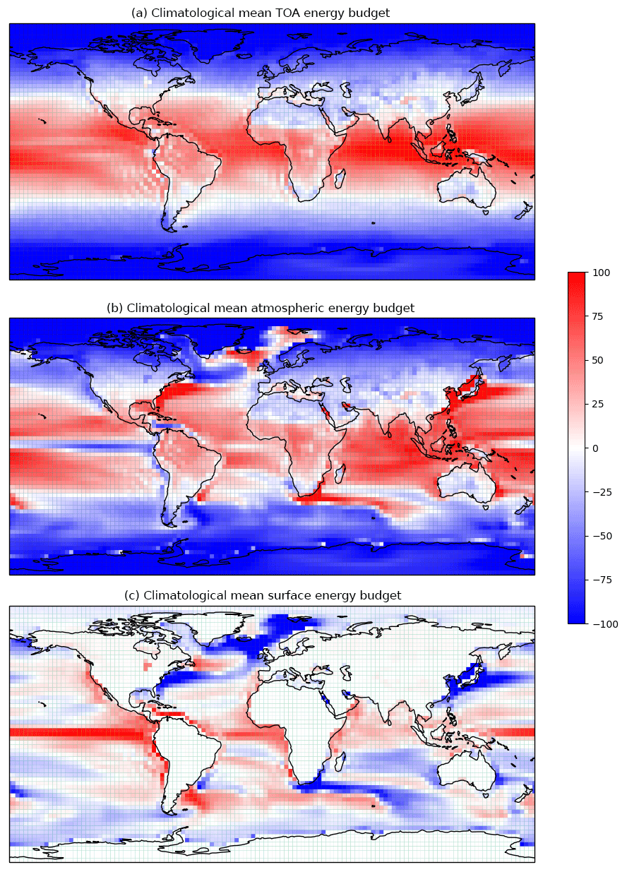
Figure 1 Climatological annual mean maps of (a) TOA, (b) atmospheric and (c) surface energy budgets for the CanESM2 model (W m⁻²). The fluxes are positive when entering the domain and negative when exiting the domain.

Let us finally consider that both the direct and the indirect methods contain crucial approximations. The two-layer assumption reduces the estimated MEP both with the direct and indirect methods, as shown by Lucarini and Pascale (2014), who investigated the coarse graining of post-processed model data. We expect that the indirect method will be particularly affected by vertical coarse graining. Furthermore, the indirect method leads to an overestimation of MEP compared to approximate estimates by Ambaum (2010), mainly because of the vertical entropy production, as already seen in Lucarini et al. (2014). The impact of considering the 3-D radiative fluxes in Eq. (11) is under investigation with a specific intermediate-complexity model.

4 Results from a CMIP5 model

A 20-year extract of a CMIP5 model (CanESM2) simulation under pre-industrial conditions is analysed in order to demonstrate the capabilities of the diagnostic tool. The datasets are retrieved from the Earth System Grid Federation (ESGF) node at the Deutsches Klimarechenzentrum (DKRZ). The run used here for the analysis is the one denoted by “r1i1p1”. From the 995-year (2015–3010) run, the 2441–2460 period was used. The choice of the sub-period is motivated by the fact that it is the only part of the run for which a 20-year subsequent dataset of the needed variables is available in the repository.

Figure 1 shows the horizontal distribution of annual mean R_t, F_a and F_s. The TOA energy budget (R_t) is relatively smooth and zonally symmetric, with an area of net energy gain over the tropics and the oceanic subtropics and energy loss elsewhere. A maximum is found over the eastern Indian–western Pacific warm pool, where the Indian monsoons develop and the emission temperature is the lowest due to deep convection. Interestingly, this pattern is somewhat opposed by the negative values of the TOA energy budget at similar latitudes over the Sahara, where the highest near-surface temperatures are found. The warm and dry conditions characterizing desert subtropical regions determine the highest thermal emission, which largely exceeds the solar input and leads to a net energy loss. The surface energy budget (F_s) is almost vanishing over the continents, given the small thermal inertia of the land surface. The largest absolute values are found in proximity to the main subsurface ocean currents. They are mainly negative in the region of the western boundary currents (Gulf Stream, Kuroshio current, Agulhas current), where the ocean's surface transfers heat to the atmosphere. They are negative over the Humboldt Current, extending deep into the Equatorial Counter Current, and to a lesser extent in proximity to the Antarctic Circumpolar Current, where the ocean's surface takes up heat from the atmosphere. The atmospheric energy budget is by definition a local balance between the TOA and surface energy budget distribution, the most remarkable feature being the minimum in coincidence with the equatorial Pacific.

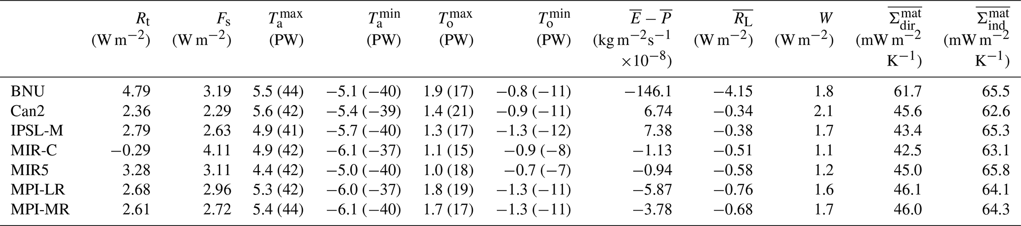
The meridional sections of climatological annual mean total, atmospheric and oceanic northward meridional enthalpy transports are shown in Fig. 2. The figure layout follows from the classic approach on meridional transports implied from budgets and their residuals (e.g. Trenberth et al., 2001; Lucarini and Ragone, 2011; Lembo et al., 2016). The transports are vanishing at the poles by definition, since the Carissimo et al. (1985) correction (in Eq. 5) is applied to account for the effect of inconsistent model energy biases. The atmospheric transport is slightly asymmetric, being stronger in the Southern Hemisphere (SH) than in the Northern Hemisphere (NH). This is closely related to the asymmetry in the mean meridional circulation, being the latitude at which the transport vanishes coincident with the annual mean position of the Intertropical Convergence Zone (ITCZ), slightly north of the Equator (Schneider et al., 2014; Adam et al., 2016). The atmospheric transport peaks at about 40^∘ in both hemispheres, slightly more poleward in the NH. The peaks mark the regions where baroclinic eddies become key in transporting energy poleward, and the zonal mean divergence of moist static energy switches sign (positive toward the Equator, negative toward the poles; see Loeb et al., 2015). The oceanic transport is much less homogeneous than the atmosphere. The two peaks are located near the subtropical and mid-latitudinal gyres, the second being smaller than the first. At mid-latitudes of the Southern Hemisphere a relative maximum is found in some models (see Fig. 8), even denoting a counter-transport from the South Pole toward the Equator. This is a critical issue, evidencing that the reproduction of the Southern Ocean circumpolar current is a major source of uncertainty in climate models (Trenberth and Fasullo, 2010).

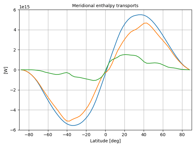
Figure 2 Climatological annual mean total (blue), atmospheric (orange) and oceanic (green) northward meridional enthalpy transports for 20 years of a pre-industrial CanESM2 model run (W).

Figure 3 Scatter plots of 20-year pre-industrial CanESM2 annual mean atmospheric vs. oceanic peak magnitudes (W) in the SH (a) and the NH (b).

Figure 3 shows the relationship between atmospheric and oceanic peak magnitudes. CanESM2 exhibits a clear relation between the two quantities in the SH. A stronger oceanic peak corresponds to a weaker atmospheric peak, whereas the relation is less clear in the NH. The anticorrelation of oceanic and atmospheric peaks suggests that the Bjerknes compensation mechanism (Bjerknes, 1969; Stone, 1978) is well reproduced by the model, confirming that the shape of the total meridional enthalpy transports is constrained by geometric and astronomical factors. This is far from being a trivial argument, since changes in the meridional planetary albedo can affect the total enthalpy transports (Enderton and Marshall, 2009), as well as the ocean–atmosphere partitioning (Rose and Ferreira, 2013). These tools facilitate an evaluation of these patterns in different models and under different scenarios and forcings.

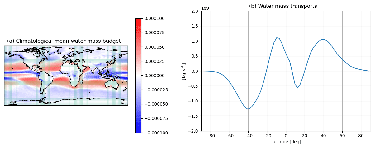
Figure 4 (a) Climatological annual mean water mass fluxes (kg m⁻² s⁻¹) and (b) annual mean northward meridional water mass transport (kg s⁻¹) for a 20-year pre-industrial CanESM2 model run.

Figure 4 shows the annual mean horizontal distribution of water vapour in the atmosphere and its zonal mean meridional northward transport. This highlights the sources and sinks of humidity in the atmosphere, evidencing that most of the exchanges are over the oceans. The water mass (and similarly the latent heat) budget is relatively weak over most of the continents with significant regional exceptions, notably the Amazon, Bengal and Indonesia, as well as parts of the western coast of the American continent. The water mass budget over these land areas is mainly negative, denoting an excess of precipitation compared to evaporation. The zonal mean water mass transport (Fig. 4b) is mainly poleward, except in the SH (30^∘ S–Equator) and the NH tropics (10–30^∘ N), essentially diverging humidity in both directions from the oceanic subtropics in both hemispheres. Water mass (and similarly latent energy, not shown) is primarily advected toward the regions of deep convection – the ITCZ (slightly north of the Equator) – and secondarily toward both hemisphere extratropics, where moisture is provided for the baroclinic eddies (see Cohen et al., 2000).

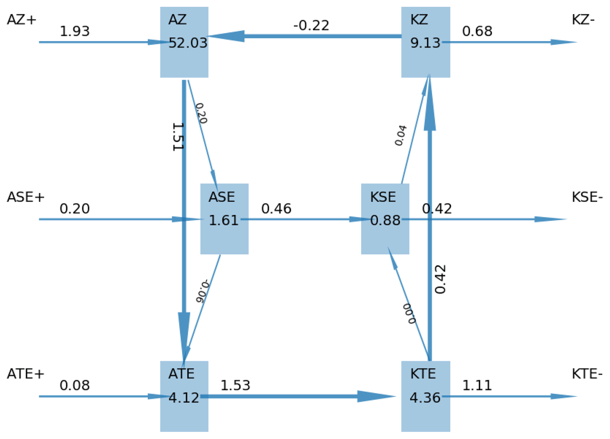
Figure 5 Diagram of Lorenz energy cycle (LEC) annual mean production, dissipation, storage and conversion terms for 1 year of the pre-industrial CanESM2 model run. AZ denotes the APE reservoir in the zonal mean flow, and ASE and ATE denote the APE associated with stationary and transient eddies, respectively. KZ denotes the KE associated with the zonal mean flow, and KSE and KTE denote the KE associated with the stationary and transient eddies (see Appendix A2). Reservoirs are displayed in units of 10⁵ joules per square metre and conversion terms as watts per square metre.

The Lorenz energy cycle for 1 year of a CanESM2 model run (Fig. 5) shows how the energetics of atmospheric dynamics are calculated by the diagnostic tool. The reservoirs of available potential energy (APE) and kinetic energy (KE) are shown in the blue boxes, separately accounting for the zonal mean, the stationary eddies (eddies in the time-averaged circulation) and the transient eddies (departure from zonal and time mean). The spectral approach also allows for a partition between planetary wavenumbers, synoptic wavenumbers and higher-order eddies (not shown here).

Most of the energy is stored in the form of APE in the zonal mean flux and to a lesser extent in the zonal mean kinetic energy. The zonal mean APE is almost instantly converted into eddy potential energy (mainly through meridional advection of sensible heat) and then into eddy kinetic energy (through vertical motions in eddies) by means of mid-latitudinal baroclinic instability, so the two conversion terms are unsurprisingly qualitatively similar. We also notice that the eddy APE and KE reservoirs have similar magnitudes. As argued before (Li et al., 2007), this is a consequence of the tight relation between temperature perturbations to the zonal mean meridional profile and the eddy synoptic activity. CanESM2 (and other models as well, not shown) agrees well with observational-based datasets that the stationary eddies play a non-negligible role in the baroclinic–barotropic energy conversion (see Ulbrich and Speth, 1991). As for the KE, the transient eddy reservoirs are about half of the zonal mean, with the stationary eddy playing a more marginal role. The barotropic conversion acts mainly by converting eddy KE into zonal mean KE (i.e. restoring the jet stream) but in part also converting APE into KE (or vice versa) in the zonal mean flow.

Compared to reanalysis datasets (e.g. Ulbrich and Speth, 1991; Li et al., 2007; Kim and Kim, 2013), our approach calculates more energy stored in the zonal mean reservoirs. This is consistent with previous findings (see Boer and Lambert, 2008; Marques et al., 2011) and is possibly due to the well-known cold pole bias and the consequently excessive speed of the jet stream. Besides the fact that pre-industrial conditions feature different conditions than the present day, as shown in Table 7, another possible explanation is that, unlike previous results from reanalysis, we only consider the tropospheric part of the Lorenz energy cycle. The conversions of APE to and from stationary eddies also diverge from reanalyses (Kim and Kim, 2013), although the overall baroclinic conversion is consistent with them. For model intercomparison in the next section, we will consider the sum of the stationary and transient eddies as a single eddy component. The KE–APE conversion in the zonal mean flow is problematic, with CanESM2 having an opposite sign to the measurements made for reanalyses, although they also appear to have certain inconsistencies (Kim and Kim, 2013).

Results obtained from the indirect method for MEP with the CanESM2 model are shown in Fig. 6, denoting climatological annual mean maps of the vertical (panel a) and horizontal component (panel b). Two different colour maps have been used in order to emphasize that, although the vertical component has smaller maximum values than the horizontal component, it is positive almost everywhere (see Lucarini et al., 2011). As mentioned in Sect. 3.4.2, the local value of the horizontal component is not meaningful per se, and this component should only be addressed globally. Figure 6b is meant to describe an entropy flux divergence from the tropics, particularly the Indian–Pacific warm pool, toward the high latitudes, roughly reflecting the atmospheric meridional enthalpy transport described in Fig. 2. This provides a link between entropy production and the meridional enthalpy transports, with the null isentrope delimiting the areas of enthalpy divergence from those of enthalpy convergence (see Loeb et al., 2015). Vertical entropy production features its highest values where evaporation is most intense (see Fig. 4a). By contrast, the lowest values are found over the continents and the regions of subsidence in the atmospheric meridional circulation. The vertical component is indicative of a local budget, in which atmospheric columns are weakly coupled with each other and mixing occurs on the vertical (Lucarini and Pascale, 2014).

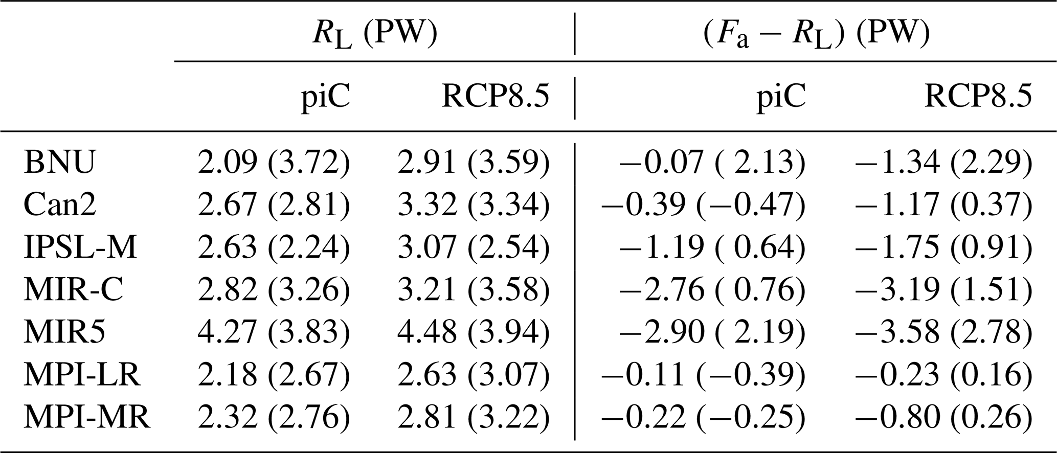
Table 2 Annual mean values of a 20-year subset of control runs from 12 models participating in CMIP5 for TOA and surface energy budgets (B_t and B_s, respectively), maximal and minimal peaks of atmospheric and oceanic meridional enthalpy transports (with peak locations in latitude degrees specified in brackets) ($T_{\text{a}}^{\text{max}}$, $T_{\text{a}}^{\text{min}}$, $T_{\text{o}}^{\text{max}}$, $T_{\text{o}}^{\text{min}}$), water mass budget ($\stackrel{\mathrm{‾}}{E}-\stackrel{\mathrm{‾}}{P}$), latent energy budget ($\stackrel{\mathrm{‾}}{R_{\text{L}}}$), mechanical work by the Lorenz energy cycle, and material entropy production computed with the direct and indirect methods ($\stackrel{\mathrm{‾}}{{\mathrm{\Sigma }}_{\text{dir}}^{\text{mat}}}$ and $\stackrel{\mathrm{‾}}{{\mathrm{\Sigma }}_{\text{ind}}^{\text{mat}}}$, respectively).

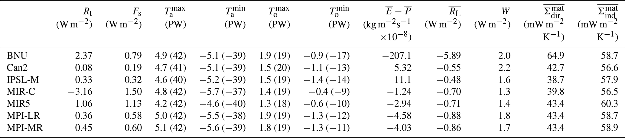
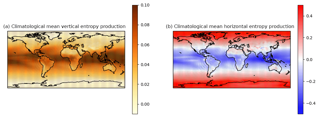
Figure 6 Climatological annual mean maps of (a) the vertical component of material entropy production (W m⁻² K) and (b) the horizontal component of material entropy production (W m⁻² K) for a 20-year pre-industrial CanESM2 model run.

5 Multi-model intercomparison and changes across different scenarios

We now focus on comparing a seven-member multi-model ensemble from CMIP5 under three different scenarios: “piControl” (piC), denoting pre-industrial conditions, “historical” (hist), i.e. a realistic forcing evolution for the 1870–2005 period, and “RCP8.5”, representing the 2005–2100 evolution of greenhouse gas (GHG) forcing under a business-as-usual emission scenario (in other words, 8.5 W m⁻² forcing by the end of the 21st century). For the piC scenario, 20-year periods, not necessarily overlapping, have been considered for each model; for the hist scenario the 1981–2000 period is considered, and for RCP8.5 the 2081–2100 period is considered. The seven models and the 20-year periods chosen are motivated by the availability of model outputs on the DKRZ ESGF node. Furthermore, this time length reflects the typical range for decadal climate predictions, as indicated in the Intergovernmental Panel on Climate Change (2013) report, so it aligns with our aim to describe the mean state and inter-annual variability of the climate system under different conditions. A summary of the main global metrics described in Sect. 3 is reported in Tables 2–4.

5.1 Energy and water mass budgets, meridional enthalpy transports

As shown in the first two columns of Table 2, there is a large imbalance in the TOA energy budget under unforced piC conditions. Such an imbalance sums up with the atmospheric energy budget imbalance (not shown, see Eq. 3), resulting in the surface energy budget estimates (the multi-model mean value for R_t being 0.21 W m⁻²; for F_s 0.73 W m⁻²). Some clear outliers are found, having either negative (BNU) or positive (MIR-C) values. This imbalance is the signature of the well-known model drift in climate models (Gupta et al., 2013). The fact that it is larger on surface budgets is explained by the fact that models are generally tuned in order to achieve vanishing TOA budgets (see Mauritsen et al., 2012; Hourdin et al., 2017), whereas surface energy budgets are often untuned. Panels a–c of Fig. 7 emphasize how these biases are relevant with respect to the inter-annual variability of the budgets (computed as the standard deviation of the annual mean values). The atmospheric inter-annual variability is roughly 1 order of magnitude smaller (about 0.1 W m⁻²) than the variability in the TOA and surface budgets, emphasizing that the changes in the overall energy imbalance are transferred to a large extent into the ocean (see also Fig. 7d). The inter-model spread on net energy fluxes is similar at the surface and at TOA, except for two models (BNU and MIR5) exhibiting a very large imbalance in the atmosphere, which is then reflected in TOA imbalance. There is limited correlation between surface and atmospheric imbalances. The inter-annual variability is roughly the same order of magnitude as the imbalances, both in the atmosphere and at the surface–TOA (about 0.20–0.25 W m⁻²).

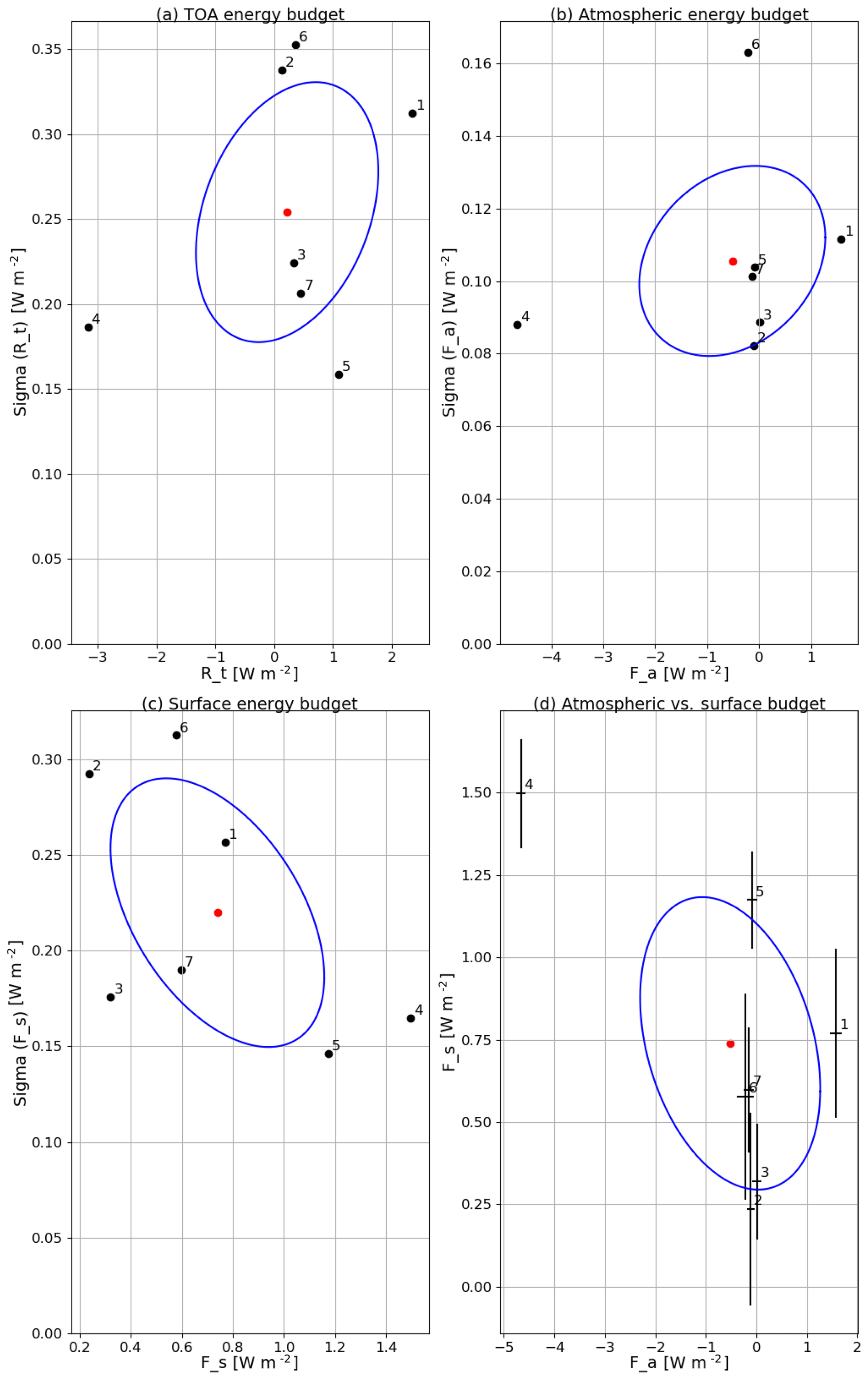
Figure 7 Multi-model ensemble scatter plots of annual mean averaged quantities vs. inter-annual variability in the piC scenario for (a) TOA energy budget, (b) atmospheric energy budget and (c) surface energy budget. Panel (d) shows the atmospheric energy budget vs. the surface energy budget, with whiskers denoting the inter-annual variability as in panels (b) and (c). Blue ellipses denote the σ standard deviation of the multi-model mean (denoted by the red dot). Model IDs are (1) BNU, (2) Can2, (3) IPSL-M, (4) MIR5, (5) MIR-C, (6) MPI-LR and (7) MPI-MR.

Table 3 Same as in Table 2 for the period 1970–2000 of the historical runs.

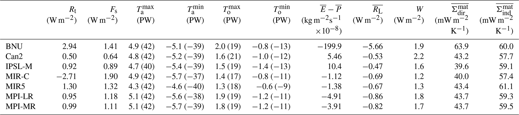
Table 4 Same as in Table 2 for the period 2071-2100 of the RCP8.5 runs.

As a consequence of a time-varying GHG forcing, the TOA imbalance increases (see Tables 3 and 4). By the end of the historical period, most models agree on a positive imbalance (with respect to unforced biased conditions), ranging between 0.2 and 0.7 W m⁻², although still in the range of the inter-annual variability (see Fig. 7a). The imbalance is much stronger by the end of the RCP8.5 period, peaking at 2.8 W m⁻² (net of the bias, i.e. the value of the imbalance in the piC scenario) in MIR-C. The surface imbalance appears to increase consistently with the TOA imbalance.

Figure 9 shows the difference in the zonal mean meridional latent heat transport between the Equator and 10^∘ N. As mentioned in Sect. 4 (see Fig. 4b), this is a measure of the moisture convergence toward the ITCZ. There is quite large uncertainty on its value in the piC scenario, ranging between 1 and 3 PW. In all models the convergence is found to increase by up to 1 PW between piC and RCP8.5. Even though it is beyond the scope of this work, this may be a robust estimate of the intensity of the uplifting branch and to some extent of the intensity of the Hadley circulation.

Table 5 Annual mean land–ocean asymmetries for atmospheric, latent energy budget and the difference of the two, for 20 years of multi-model ensemble simulations under piC conditions. Values are in watts per square metre.

Table 5 denotes a discrepancy of several watts per square metre in the atmospheric budgets over ocean and land, with a positive imbalance over the former and negative over the latter. Such a well-known imbalance (see Wild et al., 2015, for a review on the model perspective) is key to probing the model ability to reproduce the hydrological cycle, which mediates the convergence of latent energy (see Eq. 9) from oceans (where water mass evaporates) toward the continents (where a large part of it precipitates). Atmospheric and latent energy land–ocean asymmetries are compared in the first two columns of Table 5. Models that are relatively well balanced (Can2, IPSL-M, MPI-LR and MPI-MR) also feature relatively similar asymmetries. These are translated into land–ocean transports if ocean and land fluxes are multiplied by their respective surface area. The two transports are theoretically required to be of equal magnitude but opposite sign (see Table 6) and are estimated to be close to 2.8 PW (Wild et al., 2015). Few models comply with this basic energy conservation requirement (with Can2, IPSL-M, MPI-LR and MPI-MR performing better than the others); others feature differences up to 1.7 PW for BNU. For the better-performing models, note that a residual asymmetry holds, which is not attributable to the latent energy asymmetry (third column in Table 5). Those transports are directed from land toward the oceans and are interpreted as the land–ocean transports related to asymmetries in the sensible heat fluxes at the surface. The ocean–land latent energy transport is found to increase in RCP8.5 by 0.4–0.8 PW. This can be interpreted as an increase in the strength of the hydrological cycle, in line with previous findings (e.g. Levang and Schmitt, 2015). Looking at individual components of the hydrological cycle, we find an increase in both evaporation over oceans and precipitation over land.

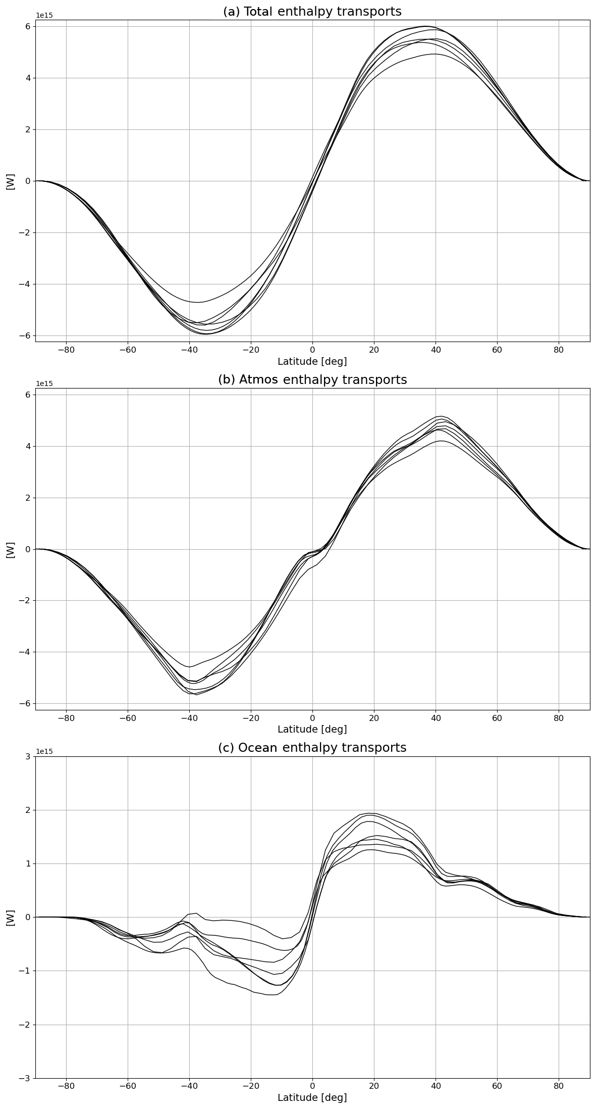
Figure 8 Climatological annual mean (a) total, (b) atmospheric and (c) oceanic northward meridional enthalpy transports for all models (W).

Figure 9 Latent heat transport between the Equator and 10^∘ N for the seven models in the three scenarios. The transport increases from piC to RCP8.5. Values are in watts and are positive if northward directed.

The mean meridional sections of total, atmospheric and oceanic enthalpy transports for each model are shown in Fig. 8 for the piC conditions alone (see Tables 2–4 for an overview of peak magnitude and position values). The choice of not showing hist and RCP8.5 is motivated by the insensitivity of enthalpy transports to the different forcing (in agreement with the theory by Bjerknes, 1969, and Stone, 1978, confirmed by previous findings on CMIP model behaviours in disparate forcings representative of present-day climate or future emission scenarios; e.g. Lucarini et al., 2011; Lembo et al., 2019a; Irving et al., 2019). Models agree on the asymmetry in the atmospheric transport, being stronger in the Southern Hemisphere than in the Northern Hemisphere (see Sect. 3). A significant source of uncertainty is the location of the zero crossing, which in some cases is very close to the Equator or even displaced in the SH. This is an important metric for the strength and shape of the mean meridional circulation. Compared to the atmosphere, the uncertainty on oceanic enthalpy transports is much larger, especially in the Southern Hemisphere, with some models featuring a counter-transport toward the Equator. As already mentioned (see Sect. 4), a typical source of uncertainty here is the relative maximum in the Southern Hemisphere extratropics.

Table 6 Evolution of land–ocean asymmetries for latent energy and for the residual of the atmospheric budget for 20 years of multi-model ensemble simulations under the two extremal scenarios (piC and RCP8.5). Values are in petawatts (PW) and are positive if they are directed toward land. Values in brackets are from spatial integration over land; those not in brackets are from integration over oceans.

5.2 The intensity of the LEC and its components

Column 11 in Tables 2–4 evidences that the intensity of the Lorenz energy cycle is relatively constant through the scenarios. Its value ranges between 2.2 W m⁻² (Can2) and 1.1 W m⁻² (MIR5 in the RCP8.5 scenario). As mentioned in Sect. 2, a major source of uncertainty is the way fields are vertically discretized in pressure levels across the different models. Some models (BNU, Can2, MPI-LR, MPI-MR) internally interpolate the fields to provide a value in each grid point at each level. Others have no values where the surface pressure is lower than the respective pressure level. This normally occurs over Antarctica and mountainous regions (most notably Himalaya and the Rocky Mountains), where the surface pressure reaches values even lower than 700 hPa. Since the LEC is computed on spectral fields, the original grid point fields have to be continuous, and any gap must be filled with a vertical interpolation. In order to do so, daily mean near-surface fields of zonal and meridional velocities as well as near-surface temperatures are used. Near-surface velocities replace the gaps, whereas near-surface temperatures are interpolated assuming a vertical profile of temperature reconstructed from barometric equations (see Sect. 3.4.1). Despite the retrieved velocity and temperature profiles being qualitatively comparable with those from the internally interpolated models, the stationary eddy conversion terms are unreasonably weaker. This is not entirely surprising, since the interpolation mostly affects mountain regions over the mid-latitudinal continents, i.e. the regions where orographically driven stationary planetary waves are generated.

The intensity of the LEC is not very sensitive to the type of forcing. The result is partially in contrast with a previous version of MPI-LR (Hernández-Deckers and von Storch, 2010) and reanalyses (Pan et al., 2017), though the changes and trends in the APE–KE conversion (i.e. the intensity of the LEC) for both studies are not very strong. Table 7 provides values of the reservoirs and conversion terms for the seven models in the three scenarios, evidencing relevant changes in some of the reservoirs across the different scenarios. Note that the zonal mean APE is largely decreased from piC to RCP8.5. This is compensated for by an increase of similar magnitude in the zonal mean KE (and, to a lesser extent, in the eddy KE). In other words, in the wake of an increasing GHG forcing, the share of kinetic energy to available potential energy is changed in favour of the first. The total (APE + KE) energy contained in all storage terms remains approximately constant, in agreement with Pan et al. (2017). These results are consistent with what was found by Hernández-Deckers and von Storch (2010) with a previous version of MPI-ESM-LR and Veiga and Ambrizzi (2013) with a state-of-the-art version of MPI-ESM-MR. The zonal mean APE reduction is consistent with a reduction of the meridional temperature gradient, which is predominantly a consequence of high-latitude warming amplification (see also Li et al., 2007). The increase in zonal mean kinetic energy reflects a strengthening of the tropospheric mid-latitude jet stream (consistent with what was previously found about the SH tropospheric jet; e.g. Wilcox et al., 2012). The impact of climate change on the mid-latitudinal eddy activity is less clear. The (slight) increase in eddy kinetic energy may reflect an increased mid-latitudinal baroclinic eddy activity in the Pacific and Atlantic storm tracks (despite large model uncertainty on this aspect; see Intergovernmental Panel on Climate Change, 2013). This, together with the rise of the tropical tropopause (mainly as a consequence of surface warming; see Lin et al., 2017), may contrast with the expected decrease in baroclinic eddy activity associated with a smaller meridional temperature gradient due to polar amplification. This approach allows us to straightforwardly associate the different response of the models to the increasing GHG with key aspects of the general circulation of the atmosphere.

5.3 Material entropy production in the two methods

The components of the material entropy production in the indirect and direct methods are closely related to each other and provide further insight into the interpretation of water mass, energy budgets and LEC results.

Table 7 Annual mean values of APE and KE reservoirs and conversion terms in the LEC (reservoir values: 10⁵ J m⁻², conversion terms: W m⁻²). For the notation, refer to Appendix A1.

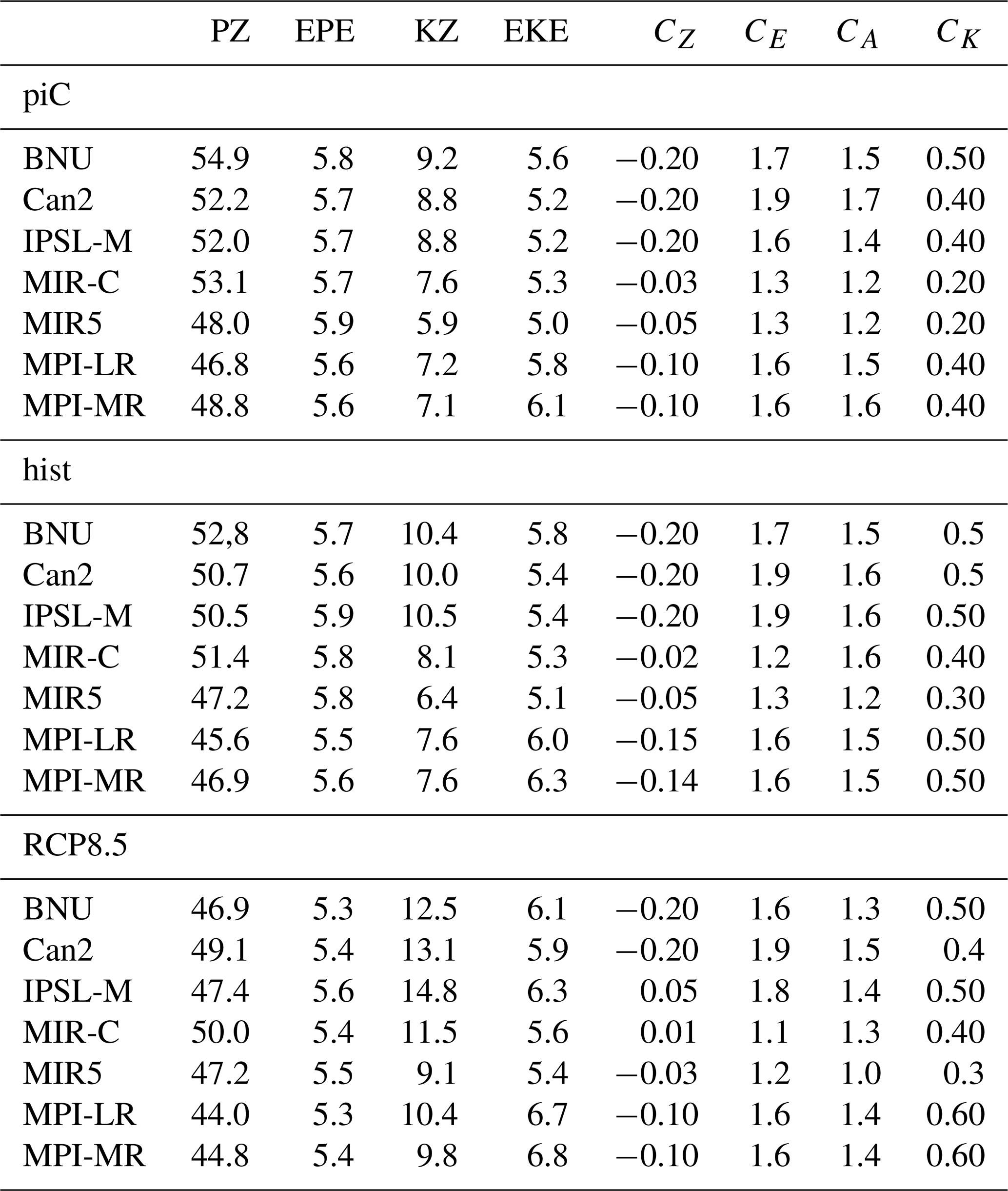
Table 8 summarizes the main components of the material entropy production in the two methods. Most of the MEP obtained with the direct method is related to the hydrological cycle. The vertical component overcomes the horizontal component in the indirect method by an order of magnitude. We have already commented on this in Sects. 3.4.2 and 4. The previous arguments about the changes in intensity of the hydrological cycle and the atmospheric circulation are reflected here as well. The entropy production increases with increasing GHG forcing in all models (except BNU, being strongly water mass and energy unbalanced). The increase in the MEP related to the hydrological cycle ranges between 2.4 mW m⁻² K⁻¹ (MIR5) and 4.7 mW m⁻² K⁻¹ (IPSL-M) from piC to RCP8.5, amounting to about a 10 % increase. The vertical component increase ranges between 5.6 mW m⁻² K⁻¹ (MPI-MR) and 7.3 mW m⁻² K⁻¹ (IPSL-M). Models showing larger increases in the hydrological-cycle-related MEP also feature a stronger increase in the vertical component. In other words, the vertical component, which is a signature of MEP related to vertical uplift, especially deep tropical convective activity, is closely relate to the strength of the hydrological cycle.

Table 8 Annual mean components of the material entropy production obtained with the direct and indirect methods. For each model, the first row denotes the estimates from piC, the second row from hist and the third row from RCP8.5 (values: mW m⁻² K⁻¹).

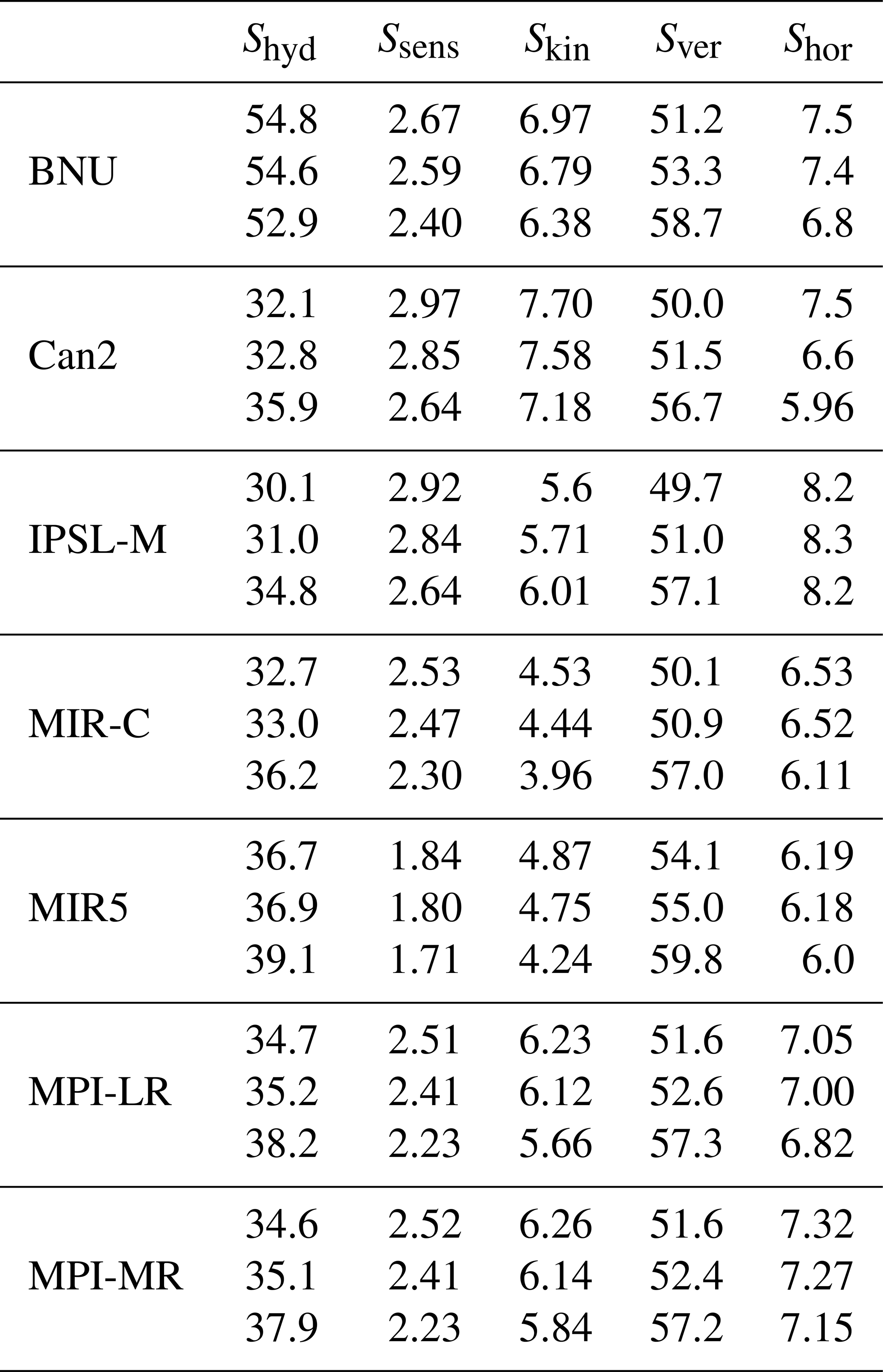
Table 9 The 20-year annual mean material entropy production associated with the hydrological cycle. Each component denotes a different process: (from left to right) evaporation, rainfall precipitation, snowfall precipitation, snow melting at the ground and the potential energy of the droplet. For each model, the first row denotes the estimates from piC, the second row from hist and the third row from RCP8.5 (values: mW m⁻² K⁻¹).

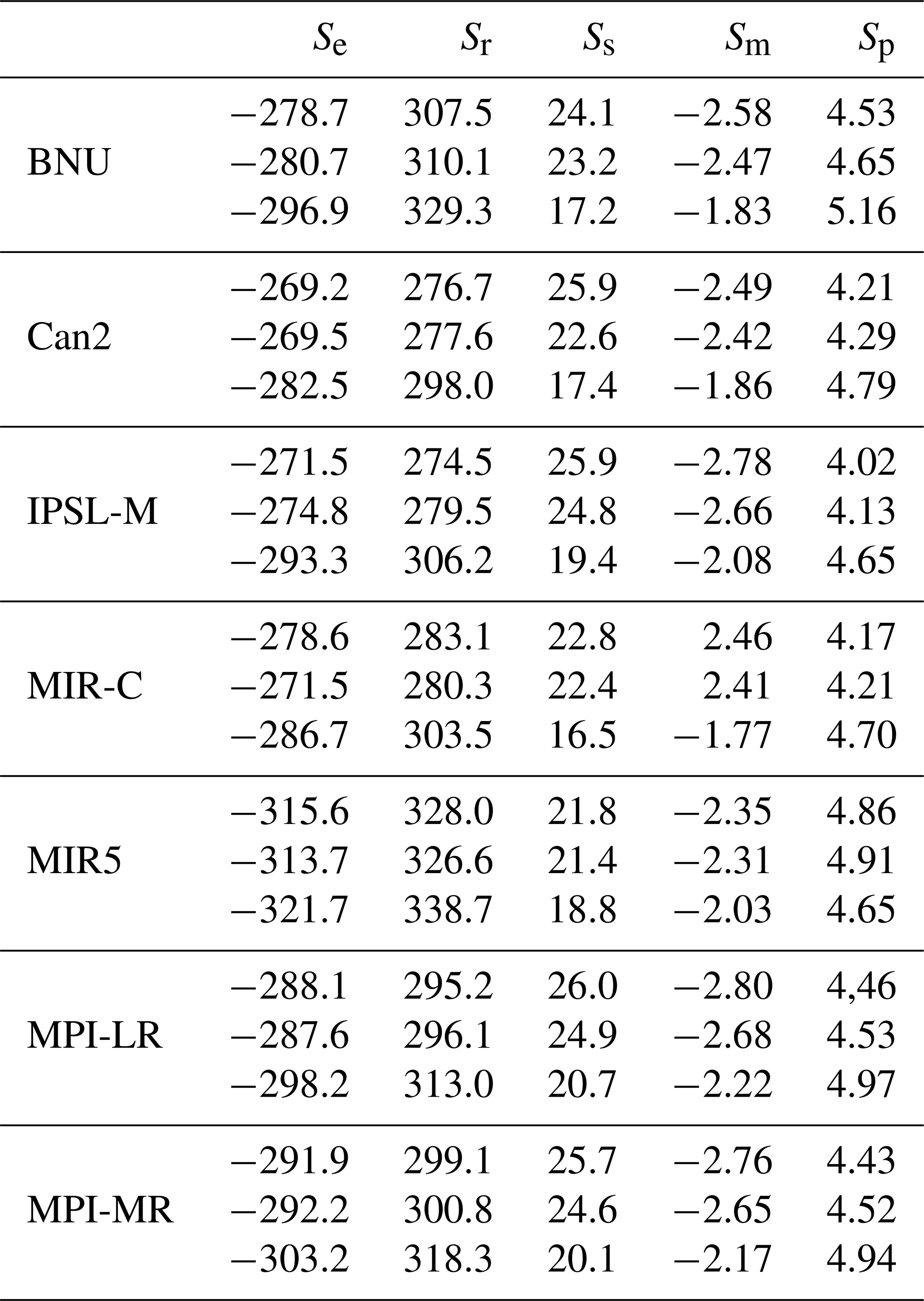
Table 9 provides more insight into the components of the MEP related to the hydrological cycle (see Eq. 15). On the one hand is the reduction in MEP due to a decrease in snowfall precipitation (S_s). This reduction ranges between 3 mW m⁻² K⁻¹ (MIR5) and 8.5 mW m⁻² K⁻¹ (BNU) from piC to RCP8.5, to which a reduction of less than 1 mW m⁻² K⁻¹ must be added to reflect a reduction in snowmelt (S_m). On the other hand, a large increase in MEP due to rainfall precipitation (S_r) is found, ranging between 10.7 mW m⁻² K⁻¹ (MIR5) and 32.1 mW m⁻² K⁻¹ (IPSL-M) from piC to RCP8.5, generally overcoming the MEP reduction related to evaporation at the surface (S_e). This increase can be interpreted in different ways: either as an increase in water mass which is precipitated or in terms of a lower working temperature for rain droplet formation (T_C). As a consequence of the water mass balance, the latent heat associated with evaporation and precipitation must equal each other (less the changes in latent heat related to snowfall precipitation and the marginal contribution by snow melting at the ground). We thus attribute such an increase in S_r to changes in T_C. This might also be indicative of a larger rate of convective precipitation on stratiform precipitation and could be investigated further.

Concerning the other terms of the MEP budget, the one related to the sensible heat fluxes at the surface is slightly reduced, whereas the kinetic energy dissipation term is increased. Given that the LEC intensity, from which the kinetic energy dissipation has been derived, is to a large extent stationary across the scenario, such change is not related to the intensification of the atmospheric circulation (see Sect. 5.2); it is rather attributable to the near-surface warming. Finally, the decrease in the horizontal component is in line with the decrease in the APE terms of the LEC (especially the zonal mean term), denoting a weaker heat convergence toward the high latitudes (mainly as a consequence of the polar amplification).

In total, the entropy production is found to increase with increasing GHG forcing (see Tables 2–4), both via the indirect and the direct method. This is consistent with previous findings (Lucarini et al., 2014, 2011) and points to the role of latent heat release in convective processes in establishing the response of the climate system. The reduction of the meridional enthalpy transports is also consistent with previous comparisons between dry and moist entropy fluxes (Laliberté and Pauluis, 2010), suggesting that the hydrological cycle affects the efficiency of the atmospheric thermal engine (Laliberté et al., 2015).

5.4 Baroclinic efficiency and irreversibility

As a wrap-up of the various aspects touched on in this section, we introduce two metrics. The first is the “baroclinic efficiency” (Lucarini et al., 2011):

$$\begin{array}{}\text{(25)}& \mathit{\eta }={\displaystyle \frac{T_{\text{E}}^{>}-T_{\text{E}}^{<}}{T_E^{>}}},\end{array}$$

where $T_{\text{E}}^{>}$ and $T_{\text{E}}^{<}$ are the emission temperatures averaged in the domains defined by TOA net energy gain and net energy loss (see Fig. 1), respectively. The second is the “degree of irreversibility” (Lucarini et al., 2011):

$$\begin{array}{}\text{(26)}& \mathit{\alpha }={\displaystyle \frac{\stackrel{\mathrm{‾}}{{\dot{S}}_{\text{dir}}^{\text{mat}}}-\stackrel{\mathrm{‾}}{{\dot{S}}_k^{\text{mat}}}}{\stackrel{\mathrm{‾}}{{\dot{S}}_k^{\text{mat}}}}},\end{array}$$

i.e. the ratio of MEP from irreversible processes other than the kinetic energy dissipation to the MEP related to the kinetic energy dissipation alone. The first parameter accounts for the strength of the mean meridional circulation driven by the differential thermal gradient. This is a measure of the dry entropy fluxes related to the heat-to-work conversion associated with the existence of the LEC and constitutes an upper limit to the efficiency of the atmospheric thermal engine. The second parameter accounts for the relevance of viscous dissipation compared to other non-viscous irreversible processes. This parameter is closely related to the Bejan number, which is widely used in thermodynamics for the study of heat transfers in a fluid (Awad, 2016).

Table 10 The 20-year annual mean irreversibility and baroclinic efficiency for each model and each scenario. Baroclinic efficiency is rescaled as 10⁻².

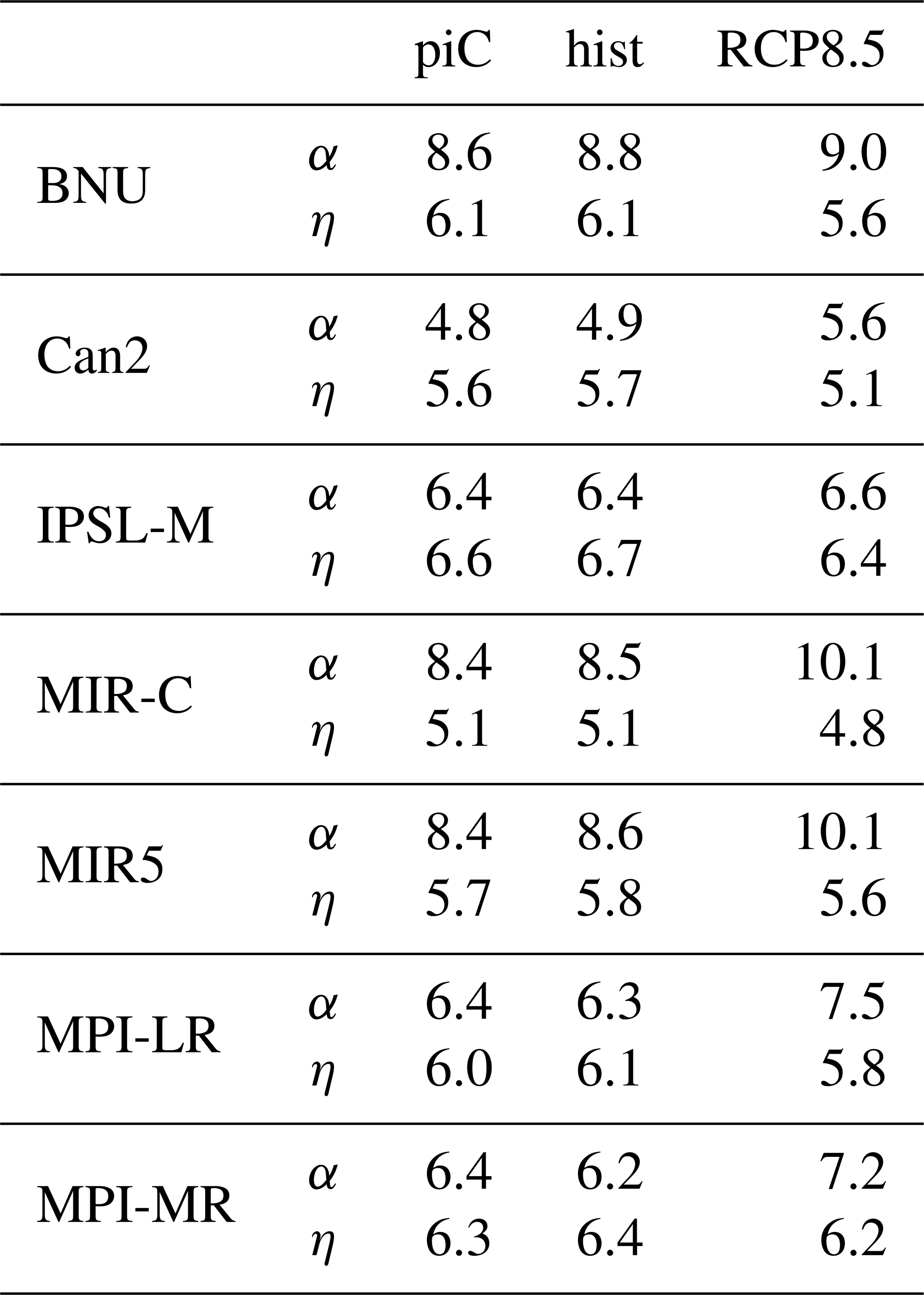
Table 10 shows the results from the three scenarios for the seven models that have been considered. The baroclinic efficiency ranges between 0.051 (MIR-C) and 0.066 (IPSL-M) in piC. It undergoes a clear reduction in the wake of increasing forcing as a consequence of the already discussed reduction in the heat convergence at high latitudes. Remarkably, the last 20 years of hist do not seem to be significantly different from piC, contrary to RCP8.5. The irreversibility, in turn, is generally increased, especially between hist and RCP8.5. As noted before, the hydrological cycle plays an increasingly significant role in converting energy into the system in a warmer climate (see also Laliberté and Pauluis, 2010; Laliberté et al., 2015). This reflects a less efficient meridional enthalpy transport from low to high latitudes and consequently a larger irreversibility of the system, as already argued in Lucarini et al. (2010a, b).

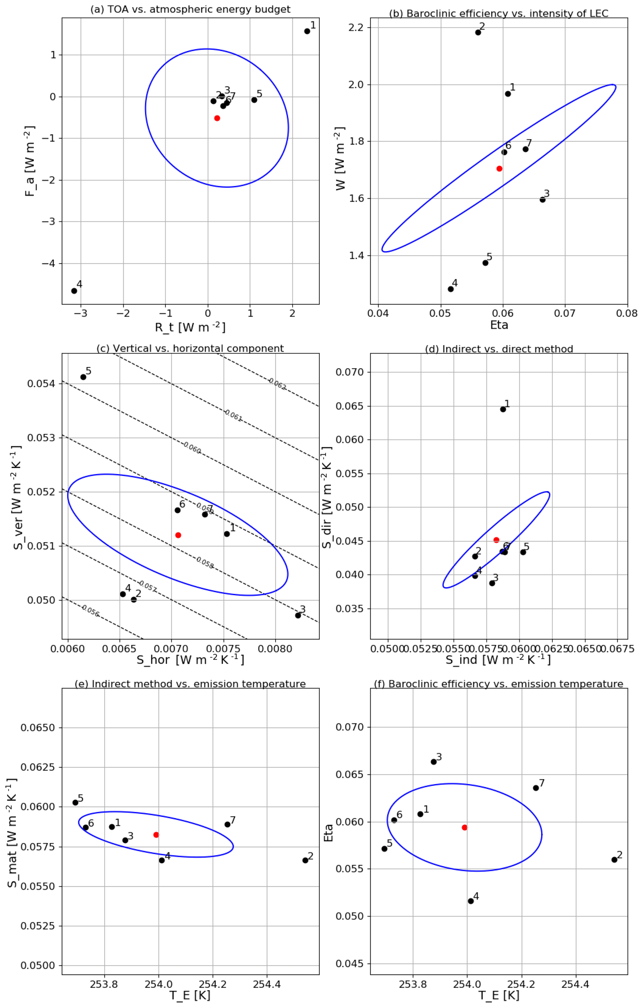
Figure 10 Multi-model ensemble scatter plots from the piC scenario for (a) atmospheric energy budget vs. TOA energy budget (W m⁻²), (b) baroclinic efficiency vs. LEC intensity (W m⁻²), (c) vertical component of the material entropy production vs. vertical component (together with isolines of total material entropy production with the indirect method) (W m⁻² K), and (d) direct vs. indirect method for material entropy production (W m⁻²K). Blue ellipses denote the σ standard deviation of the multi-model mean (denoted by the red dot). Model IDs are (1) BNU, (2) Can2, (3) IPSL-M, (4) MIR5, (5) MIR-C, (6) MPI-LR and (7) MPI-MR.

5.5 Links among the metrics

Figure 10 brings up some of the metrics discussed for the piC scenario, showing how they relate with each other. The TOA and atmospheric budgets (Fig. 10a) are strongly related, with positive–negative outliers determined by positive–negative biases in atmospheric budgets. The other models cluster around vanishing atmospheric energy imbalances and slightly positive TOA imbalances, likely reflecting the oceanic model drift.

Figure 10b shows that the uncertainty on the value of baroclinic efficiency is much smaller (10 %) than the one related to the LEC (about 50%, even though the treatment of fields in pressure levels is a critical issue here, as discussed in Sect. 5.2). The two quantities are related through the meridional enthalpy transports (see Boschi et al., 2013; Lembo et al., 2019b), which in mid-latitudes are mainly effected by baroclinic eddies. As mentioned, the strength of the baroclinic conversions in the LEC is itself a measure of the strength of the LEC. One might argue that the baroclinic efficiency peaks for certain values of the LEC intensity, but a larger ensemble would be necessary to prove or disprove such a hypothesis.

Figure 10c shows the relation between horizontal and vertical components of the MEP computed with the indirect methods (see Lucarini et al., 2014). It can be noticed that larger–smaller values of the vertical components correspond to smaller–larger values of the horizontal component. Indeed, the overall MEP ranges between about 57 and 60 mW m⁻² K⁻¹, while the vertical component alone has a 4 mW m⁻² K⁻¹ uncertainty range, suggesting that a compensation mechanism occurs somewhat between the vertical and horizontal component, i.e. between the local MEP on the vertical (especially where convection occurs) and the convergence of heat towards the high latitudes.

Finally, Fig. 10d shows the relation between MEP computed via the direct and indirect methods. Besides one outlier (BNU) all models have values for the direct method of about 40 mW m⁻² K⁻¹, whereas through the indirect method they cluster at about 57.5 mW m⁻² K⁻¹. Comparison with explicit computations by Pascale et al. (2011) suggests that the discrepancy is mainly attributable to an insufficient representation of the MEP related to the hydrological cycle (which is expected, since some intermediate phase change processes are not taken into account) and to the kinetic energy dissipation (because unphysical processes cannot be accounted for here, given the different numerical schemes of the models, leading to up to a 50 % reduction of this term).

Across metrics, this analysis emphasizes that the distribution of different models is quite far from Gaussian. The multi-model ensemble mean and variances used here are certainly useful criteria for assessing the model uncertainty, but care should be taken on the choice of the members and the behaviour of each of them.

6 Summary and conclusions

We have presented TheDiaTo v1.0, a diagnostic tool for the study of different aspects of the thermodynamics of the climate system, with a focus on the atmosphere. The goal of this diagnostic tool is to support the development, evaluation and intercomparison of climate models, as well as to help the investigation of the properties of the climate in past, current and projected future conditions. The diagnostic tool is comprised of independent modules accounting for (1) the energy budgets and transports in the atmosphere, the oceans and in the system as a whole, (2) the water mass and latent energy budgets and transports, (3) the Lorenz energy cycle, and (4) material entropy production via the direct and indirect methods. Global metrics are provided for immediate comparison between different datasets.

We provide some examples of practical use of the diagnostic tool. We have presented results obtained from a 20-year subset of CMIP5 model runs under unforced pre-industrial conditions and results from a 20-year multi-model ensemble in three different scenarios: unforced pre-industrial conditions (piC), the end of the historical period (hist) and the last 2 decades of the 21st century with a business-as-usual scenario (RCP8.5). A summary of the metrics and of the comparisons between the results obtained across models and scenarios is given in Tables 2–4 and in Fig. 10.

The energy and water mass budgets are computed locally and from these the transports are inferred, providing information about the global-scale circulation. Similarly, the material entropy production has been decomposed in a component which essentially accounts for a local budget on the vertical and another one which accounts for the global meridional enthalpy transport. In other words, the metrics link the local features of the climate to the global energy and mass exchange, allowing for the evaluation of the global impact of localized changes.

We have shown how the tool can provide a comprehensive view of the dynamics of the climate system and its response to perturbations. It facilitates the evaluation of the spatial distributions of model biases and their impacts and the interpretation of the changing properties of the system with time in the reduced space defined by the considered metrics.

Apart from the specific – yet important – problem of looking into climate change scenarios, it is also straightforward to use the diagnostic tool to study paleoclimates, investigate tipping points and study the climate under varied astronomical factors or chemical compositions of the atmosphere. One can envision adapting the model for the analysis of the properties of Earth-like exoplanets.

The requirement of flexibility, which allows the tool to be easily applied to a large class of models, inevitably leads to some simplifying hypotheses. The most relevant are the following: (a) the quasi-steady-state assumption; (b) the hydrostatic assumptions as background to the LEC framework; and (c) the identification of the emission temperature as the characteristic temperature in the atmosphere, leading to the 2-D formulation of the material entropy production with the indirect method. Other assumptions involve the analysis of the hydrological cycle, in which the latent heat of evaporation and solidification has been assumed to be constant, even though its value depends on temperature and pressure. Further, it is worth noticing (Loeb et al., 2015) that the latent energy associated with snowfall melting over sea-ice-covered regions is not accounted for in CMIP5 models. This accounts for about 0.1–0.5 W m⁻². Nevertheless, unlike the water mass budget the latent energy budget is not expected to be closed, since the surface melting is not taken into account (although it is considered for the entropy budget).

Thus far, we have pointed out that the thermodynamic point of view can be linked to fundamental aspects of the atmospheric dynamics. We have related the idea of a baroclinic heat engine (Barry et al., 2002) to the mechanical work carried in a Lorenz energy cycle (Lorenz, 1955), along the lines of what was proposed by Lucarini et al. (2010a, 2014). A deeper insight into the energetics of the atmospheric dynamics would require an evaluation of the meridional mass streamfunctions. To this end, an additional diagnostic tool for the streamfunctions is under development, which uses moist and dry isentropes, rather than isobaric coordinates, following from Laliberté et al. (2015) and Kjellsson (2015), to link the Lagrangian and the Eulerian point of view. This approach is contingent on the availability of model outputs. We have shown here how deeply the hydrological cycle is affected by changes in the mean state of the system, so an isentropic approach would allow us to resolve the heat exchanges due to moist processes.

Another open issue is assessing the relevance of coarse graining for the results, not only on the material entropy production (as discussed by Lucarini and Pascale, 2014), but also in terms of LEC and efficiency (when it comes to the type of vertical discretization of the model). On the one hand, the method is being tested with 3-D fields for the radiative fluxes. On the other hand, the impact of changing the temporal, vertical and horizontal resolution is being assessed through a number of dedicated sensitivity studies in an intermediate-complexity atmospheric model.

Appendix A: Sources, sinks and conversion terms of the Lorenz energy cycle

A1 Symbols and definitions

cp	specific heat at constant pressure
g	gravity
p	pressure
r	Earth's radius
t	time
T	temperature
TV	virtual temperature
u	zonal velocity
v	meridional velocity
ω	vertical velocity
γ	$-\frac{R}{p}{\left(\frac{\partial }{\partial p}\left[\stackrel{\mathrm{‾}}{T}\right]-\frac{\partial }{\partial p}\frac{\left[\stackrel{\mathrm{‾}}{T}\right]}{p}\right)}^{-\mathrm{1}}$
$\stackrel{\mathrm{‾}}{x}$	time mean of x
x′	deviation from time mean
x	global horizontal mean
[x]	zonal mean
x*	deviation from zonal mean

A2 Storage terms

• PZ: $\frac{\mathit{\gamma }}{\mathrm{2}g}{\left(\left[\stackrel{\mathrm{‾}}{T}\right]-\mathit{\left\{}\stackrel{\mathrm{‾}}{T}\mathit{\right\}}\right)}^{\mathrm{2}}$

• EPE: $\frac{\mathit{\gamma }}{\mathrm{2}g}\left(\left[\stackrel{\mathrm{‾}}{T^{*\mathrm{2}}}\right]+\left[\stackrel{\mathrm{‾}}{{T^{\prime }}^{\mathrm{2}}}\right]\right)$

• KZ: $\frac{\mathrm{1}}{\mathrm{2}g}\left([\stackrel{\mathrm{‾}}{u}{]}^{\mathrm{2}}+[\stackrel{\mathrm{‾}}{v}{]}^{\mathrm{2}}\right)$

• EKE: $\frac{\mathrm{1}}{\mathrm{2}g}\left[\stackrel{\mathrm{‾}}{u^{*\mathrm{2}}}+\stackrel{\mathrm{‾}}{v^{*\mathrm{2}}}+\stackrel{\mathrm{‾}}{{u^{\prime }}^{\mathrm{2}}}+\stackrel{\mathrm{‾}}{{v^{\prime }}^{\mathrm{2}}}\right]$

The contribution of eddies to APE (EPE) and KE (EKE) consists of two terms; the first one is the term accounting for stationary eddies (ASE and KSE in the diagrams in Fig. 5, respectively). The second term accounts for the transient eddies (ATE and KTE in the diagrams in Fig. 5, respectively). A discussion on the derivation of these terms is found in Ulbrich and Speth (1991).

A3 Conversion terms

$$\begin{array}{rl}& C_A=\\ & -{\displaystyle \frac{\mathit{\gamma }}{g}}\left\{{\displaystyle \frac{\partial \left[\stackrel{\mathrm{‾}}{T}\right]}{r\partial \mathit{\varphi }}}\left[\stackrel{\mathrm{‾}}{v^{\prime }{T}^{\prime }}+{\stackrel{\mathrm{‾}}{v}}^{*}{\stackrel{\mathrm{‾}}{T}}^{*}\right]+\left[\stackrel{\mathrm{‾}}{{\mathit{\omega }}^{\prime }{T}^{\prime }}+{\stackrel{\mathrm{‾}}{\mathit{\omega }}}^{*}{\stackrel{\mathrm{‾}}{T}}^{*}\right]\right.\\ & \left.\left({\displaystyle \frac{\partial }{\partial p}}\left(\right[\stackrel{\mathrm{‾}}{T}]-\mathit{\{}\stackrel{\mathrm{‾}}{T}\mathit{\left\}}\right)-{\displaystyle \frac{R}{p{c}_{\text{p}}}}\left(\right[\stackrel{\mathrm{‾}}{T}]-\mathit{\{}\stackrel{\mathrm{‾}}{T}\mathit{\left\}}\right)\right)\right\}\\ & +{\displaystyle \frac{\mathit{\gamma }}{g}}\left\{+{\stackrel{\mathrm{‾}}{u^{\prime }{T}^{\prime }}}^{*}{\displaystyle \frac{\mathrm{1}}{r\cos \mathit{\varphi }}}{\displaystyle \frac{\partial {\stackrel{\mathrm{‾}}{T}}^{*}}{\partial \mathit{\lambda }}}+{\stackrel{\mathrm{‾}}{v^{\prime }{T}^{\prime }}}^{*}{\displaystyle \frac{\partial {\stackrel{\mathrm{‾}}{T}}^{*}}{r\partial \mathit{\varphi }}}\right\}\\ & C_Z=-{\displaystyle \frac{R}{gp}}\left(\left[\stackrel{\mathrm{‾}}{\mathit{\omega }}\right]-\mathit{\left\{}\stackrel{\mathrm{‾}}{\mathit{\omega }}\mathit{\right\}}\right)\left(\left[\stackrel{\mathrm{‾}}{T_v}\right]-\mathit{\left\{}\stackrel{\mathrm{‾}}{T_v}\mathit{\right\}}\right)\\ & C_E=-{\displaystyle \frac{R}{gp}}\left[{\stackrel{\mathrm{‾}}{\mathit{\omega }}}^{*}{\stackrel{\mathrm{‾}}{T_v}}^{*}+\stackrel{\mathrm{‾}}{{\mathit{\omega }}^{\prime }{T}_v^{\prime }}\right]\\ & C_K=-{\displaystyle \frac{\mathrm{1}}{g}}\left\{\left({\displaystyle \frac{\partial \left[\stackrel{\mathrm{‾}}{u}\right]}{r\partial \mathit{\varphi }}}+\left[\stackrel{\mathrm{‾}}{u}\right]{\displaystyle \frac{\tan \mathit{\varphi }}{r}}\right)[{\stackrel{\mathrm{‾}}{u}}^{*}{\stackrel{\mathrm{‾}}{v}}^{*}+\stackrel{\mathrm{‾}}{u^{\prime }{v}^{\prime }}]+{\displaystyle \frac{\partial \left[\stackrel{\mathrm{‾}}{v}\right]}{r\partial \mathit{\varphi }}}\right.\\ & [{\stackrel{\mathrm{‾}}{v}}^{*}{\stackrel{\mathrm{‾}}{v}}^{*}+\stackrel{\mathrm{‾}}{v^{\prime }{v}^{\prime }}]-{\displaystyle \frac{\tan \mathit{\varphi }}{r}}\left[\stackrel{\mathrm{‾}}{v}\right][{\stackrel{\mathrm{‾}}{u}}^{*}{\stackrel{\mathrm{‾}}{u}}^{*}+\stackrel{\mathrm{‾}}{u^{\prime }{u}^{\prime }}]+{\displaystyle \frac{\partial \left[\stackrel{\mathrm{‾}}{u}\right]}{\partial p}}[{\stackrel{\mathrm{‾}}{\mathit{\omega }}}^{*}{\stackrel{\mathrm{‾}}{u}}^{*}+\stackrel{\mathrm{‾}}{{\mathit{\omega }}^{\prime }{u}^{\prime }}]\\ & \left.+{\displaystyle \frac{\partial \left[\stackrel{\mathrm{‾}}{v}\right]}{\partial p}}[{\stackrel{\mathrm{‾}}{\mathit{\omega }}}^{*}{\stackrel{\mathrm{‾}}{v}}^{*}+\stackrel{\mathrm{‾}}{{\mathit{\omega }}^{\prime }{v}^{\prime }}]\right\}+{\displaystyle \frac{\mathrm{1}}{g}}\left\{{\stackrel{\mathrm{‾}}{u^{\prime }{u}^{\prime }}}^{*}{\displaystyle \frac{\mathrm{1}}{r\cos \mathit{\varphi }}}{\displaystyle \frac{\partial {\stackrel{\mathrm{‾}}{u}}^{*}}{\partial \mathit{\lambda }}}+{\stackrel{\mathrm{‾}}{u^{\prime }{v}^{\prime }}}^{*}\right.\\ & \left({\displaystyle \frac{\partial {\stackrel{\mathrm{‾}}{u}}^{*}}{r\partial \mathit{\varphi }}}+{\stackrel{\mathrm{‾}}{u}}^{*}{\displaystyle \frac{\tan \mathit{\varphi }}{r}}+{\displaystyle \frac{\mathrm{1}}{r\cos \mathit{\varphi }}}{\displaystyle \frac{\partial {\stackrel{\mathrm{‾}}{v}}^{*}}{\partial \mathit{\lambda }}}\right)\\ & +\left.{\stackrel{\mathrm{‾}}{v^{\prime }{v}^{\prime }}}^{*}{\displaystyle \frac{\partial {\stackrel{\mathrm{‾}}{v}}^{*}}{\partial \mathit{\varphi }}}-[\stackrel{\mathrm{‾}}{u^{\prime }{u}^{\prime }}{]}^{*}{\stackrel{\mathrm{‾}}{v}}^{*}{\displaystyle \frac{\tan \mathit{\varphi }}{r}}\right\}\end{array}$$

The curly brackets in C_A and C_K emphasize that the diagnostic module is able to distinguish between two components, one dealing with the conversion to and from zonal mean flow to and from eddy flow (first bracket) and the other dealing with the conversion among eddies (second bracket).

The source and sink terms, i.e. the generation and dissipation of APE and KE, are computed as residuals of the conversion terms at each reservoir.