the Creative Commons Attribution 4.0 License.
the Creative Commons Attribution 4.0 License.
 | 19 Aug 2019
Global simulation of semivolatile organic compounds – development and evaluation of the MESSy submodel SVOC (v1.0)
Mega Octaviani
Holger Tost
The new submodel SVOC for the Modular Earth Submodel System (MESSy) was developed and applied within the ECHAM5/MESSy Atmospheric Chemistry (EMAC) model to simulate the atmospheric cycling and air–surface exchange processes of semivolatile organic pollutants. Our focus is on four polycyclic aromatic hydrocarbons (PAHs) of largely varying properties. Some new features in input and physics parameterizations of tracers were tested: emission seasonality, the size discretization of particulate-phase tracers, the application of poly-parameter linear free-energy relationships in gas–particle partitioning, and re-volatilization from land and sea surfaces. The results indicate that the predicted global distribution of the 3-ring PAH phenanthrene is sensitive to the seasonality of its emissions, followed by the effects of considering re-volatilization from surfaces. The predicted distributions of the 4-ring PAHs fluoranthene and pyrene and the 5-ring PAH benzo(a)pyrene are found to be sensitive to the combinations of factors with their synergistic effects being stronger than the direct effects of the individual factors. The model was validated against observations of PAH concentrations and aerosol particulate mass fraction. The annual mean concentrations are simulated to the right order of magnitude for most cases and the model well captures the species and regional variations. However, large underestimation is found over the ocean. It is found that the particulate mass fraction of the benzo(a)pyrene is well simulated, whereas those of other species are lower than observed.
- Article
(6150 KB) - Full-text XML
-
Supplement
(27340 KB) - BibTeX
- EndNote


The atmospheric cycling of semivolatile organic compounds (SOCs) is particularly complex because of partitioning across phases and air–surface exchange processes, including multihopping (or “grasshopper effect”; Semeena and Lammel, 2005) and accumulation in ground compartments such as seawater, soil, vegetation, and ice/snow. Many SOCs do resist degradation in environmental compartments, and hence are persistent. In the regulation of chemical substances and in international chemicals legislation (e.g., UNEP, 2017), model-based quantifications of the overall environmental residence times (persistence) and the long-range transport potentials are requested or encouraged to be applied.
Global and regional distribution and transport of SOCs has been studied using multimedia fate (box) models and chemistry transport models (CTMs) (Scheringer and Wania, 2003). The multimedia models describe the whole or part of the globe as a few zones of homogeneous environmental characteristics (Wania and Mackay, 1999; Mackay, 2010). These models are used as tools to assess the influences of environmental parameters and change in pollutant levels in multiple compartments (Dalla Valle et al., 2007; MacLeod et al., 2005; Lamon et al., 2009). On the other hand, CTMs generally imply the application of three-dimensional Eulerian models coupled with surface and chemistry modules (e.g., Ma et al., 2003; Hansen et al., 2004; Malanichev et al., 2004; Gusev et al., 2005; Semeena et al., 2006; Gong et al., 2007; Friedman and Selin, 2012; Galarneau et al., 2014; Shrivastava et al., 2017). The addition of a surface module aims to describe air–surface exchange processes and biogeochemical cycles of contaminants, whereas a chemistry module describes the changes in air concentrations due to phase partitioning and chemical transformations. Compared to the multimedia models, CTMs have better spatial and temporal resolutions but require more computational effort. They are suitable for use to investigate the variability and episodic character of environmental fate and transport. To date, pollutants addressed in model studies were persistent organic pollutants, such as dichlorodiphenyltrichloroethane (DDT), polychlorinated biphenyls (PCBs), hexachlorocyclohexanes (HCHs), polycyclic aromatic hydrocarbons (PAHs), and more recent so-called emerging pollutants (e.g., MacLeod et al., 2011).
The sensitivity of distributions to specific processes of SOC cycling and related input parameters has been the focus of CTM-based studies (Semeena et al., 2006; Sehili and Lammel, 2007; Friedman and Selin, 2012; Galarneau et al., 2014; Thackray et al., 2015). Sehili and Lammel (2007), for instance, suggest that the gas–particle partitioning and particulate-phase oxidation scenarios have significant influences on the long-range atmospheric transport of PAHs. This finding is supported by Friedman and Selin (2012), who furthermore concluded that the effects are higher than those of irreversible partitioning and of increased aerosol concentrations.
This study presents the new multicompartment module (submodel) SVOC for the Modular Earth Submodel System (MESSy; Jöckel et al., 2006, 2010). MESSy provides a modular framework for simulations accounting for various degrees of complexity and to facilitate continuous future submodel improvements. The submodel has been applied using the general circulation model ECHAM5 (Roeckner et al., 2003, 2006) as a base model. In connection with the ECHAM5/MESSy Atmospheric Chemistry (EMAC) model, SVOC encompasses a 3-D atmosphere and 2-D surface compartments (soil, vegetation, snow, and ocean mixed layer), and considers multicompartment fate and exchange processes, such as emission, phase partitioning, wet and dry deposition of gases and particles, degradation, and air–surface gas exchange, including re-volatilization. SVOC is developed and intended to be applied for the study of all potentially re-volatilizing and gas–particle-partitioning (hence semivolatile) compounds. Nevertheless, the focus of this submodel development is the global distribution of four PAH species of largely varying properties. PAHs enter the atmospheric environment as by-products of all technological combustion processes (Shen et al., 2013) and of open fires (Gullett et al., 2008). They are ubiquitous pollutants of particular environmental and health concern (WHO, 2003; Laender et al., 2011; Lammel, 2015) and due to their continuous global emissions. Here we describe the submodel development, compare the results to observations, and assess the significance of four model features to PAH distributions and fate. These features are the temporal resolution of emissions, the size discretization of particulate-phase tracers (bulk or modal), the choice of the gas–particle partitioning scheme, and re-volatilization from surfaces.
2.1 Model descriptions
The global model applied in this study is the ECHAM5/MESSy Atmospheric Chemistry Climate model (EMAC), a three-dimensional Eulerian model for the simulations of meteorological variables, gases, aerosols, clouds, and other climate-related parameters. EMAC combines the general circulation model ECHAM5 (here version 5.3.02) (Roeckner et al., 2003, 2006) with the Modular Earth Submodel System (MESSy version 2.50; Jöckel et al., 2006, 2010). The atmospheric component of ECHAM5 derives four prognostic variables, namely vorticity, divergence, temperature, and the logarithm of surface pressure in truncated series of spherical harmonics, whereas specific humidity, cloud water, and cloud ice are represented in grid point space. MESSy provides a modular framework to define atmospheric dynamics, chemistry, transport, and radiative transfer processes. For a more detailed description of the EMAC model, evaluation and relevant studies, refer to Jöckel et al. (2006, 2010) and http://www.messy-interface.org (last access: 12 July 2019). The list of MESSy process-based modules, hereinafter submodels, applied in this study are summarized in Table 1.
Lauer et al. (2007)Pozzer et al. (2006)Roeckner et al. (2006)Tost et al. (2006b, 2010)Tost (2006)Kerkweg et al. (2006a)Pringle et al. (2010)Landgraf and Crutzen (1998)Tost et al. (2007)Sander et al. (2011)Kerkweg et al. (2006b)Kerkweg et al. (2006b)Roeckner et al. (2006); Jöckel et al. (2006)Tost et al. (2006a)Kerkweg et al. (2006a)
The new MESSy submodel SVOC for simulating the fate and cycling of SOCs in the global environment is presented. Processes involved in the submodel include gas–particle partitioning, volatilization from the surface, dry and wet depositions, and chemical and biotic degradations. These processes are connected to other MESSy submodels. For example, deposition of gas-phase SOCs are calculated by the submodels SCAV and DDEP, aerosol microphysics by GMXe, gas-phase chemistry mechanisms by MECCA, and ocean–air flux exchange by AIRSEA. Figure 1 illustrates the SVOC structure within the EMAC system and its interactions with other MESSy submodels. More details on some process parameterizations are given in the following section. A user manual can be found in the Supplement with the list of submodel input and output variables.

Figure 1Overview of EMAC-SVOC model structure, the cycling processes in SVOC submodel, and its interaction with other MESSy submodels. SMIL (submodel interface layer) and SMCL (submodel core layer) are components of MESSy coding standard, see Jöckel et al. (2006) for further details.
2.2 Parameterizations of cycling processes in multiple compartments
2.2.1 Representation of SOC in particulate phase
The parameterizations of aerosol microphysical processes for SOCs such as gas-to-particle partitioning and dry and wet deposition depend on the way the particulate phase is represented in the model. Here, there are two approaches employed in the submodel to represent the particulate-phase SOC: (1) it is assumed as a bulk species or (2) the particle sizes are resolved into n continuous (modal) distributions. The former will be hereinafter referred to as the bulk scheme and the latter referred to as the modal scheme. In the modal scheme, n is equal to the seven log-normal modes of the GMXe submodel, four with hydrophilic coating (ns: nucleation soluble, ks: Aitken soluble, as: accumulation soluble, cs: coarse soluble) and three hydrophobic (ki: Aitken insoluble, ai: accumulation insoluble, ci: coarse insoluble) (Pringle et al., 2010). Each mode is treated as an individual tracer.
2.2.2 Partitioning between gas phase and particulate phase
Gas–particle partitioning is assumed to take place when SOC is in equilibrium between the gas and particulate phases. The concentration of the species that is bound to particles (Cparticle) is calculated with
and the particulate mass fraction (θ) is defined as
where CPM is the concentration of particulate matter or PM (µg m−3), Kp is the temperature-dependent particle–air partition coefficient (m3 µg−1), and is the dimensionless Kp.
In a model configuration using size-resolved particles (viz. the modal scheme), each SOC tracer is introduced in the model as eight different species: seven aerosol particles in ns, ks, as, cs, ki, ai, ci modes and one in the gas phase. The particulate fraction of the species in mode i (θi) is calculated using Eq. (2) with and being the PM mass concentration and aerosol–air partition coefficient in the corresponding mode, respectively. The gaseous concentration Cgas is calculated using the sum of Kp values across modes, as well as total Cparticle and CPM:
It is noted that this approach may not hold the constraint of mass consistency and is thus subject to further corrections. For the current study, the effects from this problem are expected to be minimal, given the fact that PAHs in the particulate phase are mainly distributed in the accumulation mode (Lammel et al., 2010, and references therein).
For Kp calculation four options of gas–particle partitioning schemes are available in SVOC: (1) a parameterization that is based on adsorption onto aerosol surface (Junge, 1977; Pankow, 1987), (2) absorption into organic matter (Finizio et al., 1997), (3) a combination of the two ways of organic matter absorption and black carbon adsorption (Lohmann and Lammel, 2004), and (4) multiple phases of the two-way sorption system (Goss and Schwarzenbach, 2001; Endo and Goss, 2014; Shahpoury et al., 2016). Two schemes used in this study are described below.
-
Lohmann–Lammel scheme. The Lohmann–Lammel scheme takes into account an adsorption onto black carbon (BC) surface in addition to absorption into organic matter (OM) (Lohmann and Lammel, 2004). This dual-sorption theory empirically calculates Kp according to the following relation,
where ρBC is the density of BC (assumed as 1 kg L−1), ρoct is the density of octanol (0.82 kg L−1 at 20 ∘C), Ksa is the partition coefficient between diesel soot and air, aatm-BC is the available surface of atmospheric BC (m2 g−1), and asoot is the specific surface area of diesel soot (m2 g−1). The adsorptive properties of diesel soot are selected to represent the atmospheric BC because this material is considered the most significant type of BC in polluted air.
The Ksa value is calculated as a function of sub-cooled liquid vapor pressure using an estimate suggested by van Noort (2003),
where asoot in the model is set as 18.21 m2 g−1.
-
Poly-parameter linear free-energy relationships (ppLFER) scheme. The concept of poly-parameter linear free-energy relationships (ppLFER) for the prediction of equilibrium partition coefficients is introduced by Goss and Schwarzenbach (2001), and its application in environmental chemistry has been reviewed by Endo and Goss (2014). This approach can describe a composite of different types of interactions between gas-phase species and aerosols. In contrast, single-parameter LFERs only correlate the partition coefficient to the sub-cooled liquid vapor pressure or the octanol–air partition coefficient of the species, and hence only valid within the group of compounds for which they were developed.
In the study, the ppLFER scheme is incorporated into SVOC in which it defines Kp as the sum of individual partition coefficients representing surface adsorption and bulk-phase absorption processes to inorganic and organic aerosols. The formulation of Kp is adopted from Shahpoury et al. (2016) and is described as follows
where KEC, , and KNaCl are the substance partition (adsorption) coefficients () for elemental carbon or diesel soot, ammonium sulfate, and sodium chloride aerosol surface–air systems, respectively. KDMSO is the substance partition (absorption) coefficient for the dimethyl sulfoxide–air system (). KPU is the substance partition (absorption) coefficient for the polyurethane–air system (). Khexadecane is the substance partition (absorption) coefficient for the hexadecane–air system (); aEC, , and aNaCl are the adsorbent-specific surface areas: 18.21, 0.1, and 0.1 , respectively. ρDMSO and ρhexadecane are the dimethyl sulfoxide and hexadecane densities of 1.1×10⁶ and 0.77×10⁶ g m−3, respectively. CEC, , CNaCl, CWSOM, CWIOM are the concentration () of elemental carbon (here black carbon), ammonium sulfate, sodium chloride, water-soluble organic matter, and water-insoluble organic matter, respectively.
The ppLFER scheme calculates the sorptive partition coefficient for every aerosol system, as summarized in Table S1 in the Supplement. Each coefficient requires information on system parameters (e, s, a, b, v, l), and the constant c, as shown in Table S2. The Abraham solute descriptors (E, S, A, B, V, and L) are substance specific; for the species selected in this study, refer to Table S6. All the predicted partition constants are adjusted to environmental temperature using the van 't Hoff equation
where ΔH is the enthalpy of solvent–air phase transfer in joules per mole (J mol−1). This variable is system specific and calculated by applying the ppLFER equations given in Table S3 and input parameters given in Table S4. The sequence of Kp calculation from ppLFER analysis in SVOC is illustrated in Fig. S1 in the Supplement.
2.2.3 Volatilization
-
Soil
For soil volatilization, two parameterization schemes are implemented in the SVOC submodel: the Jury scheme (Jury et al., 1983, 1990) and the Smit scheme (Smit et al., 1997). The latter was applied in the study which is based on the volatilization of pesticides from the surface of fallow soils (Smit et al., 1997). The volatilization occurs upon partitioning over three soil phases (solid, gas, and liquid). The concentration of the chemical in the soil system (kg m−3) is formulated as
and the capacity factor Q is given by
where ψ and φ are the volume fractions of air and moisture, respectively; ρsoil is the soil density; Kwa is the water–air partition coefficient where ; and Ksl is the solid–liquid partition coefficient. Kaw is calculated based on the Henry's law constant:
where H is the temperature-adjusted Henry coefficient (M atm−1), R is the dry air gas constant (8.314 ), T is the environment temperature (K), ΔHsoln is the enthalpy of dissolution (J mol−1).
Ksl can be set equal to the sorption coefficient to soil organic matter Kom times the fraction of organic carbon in soil . Since Kom data are not available, the coefficient for sorption to soil organic carbon Koc was used to estimate Ksl:
Mackay and Boethling (2000) has suggested a reasonably good regression relationship between Koc and octanol–water partition coefficient Kow for PAHs:
where the factor of 1000 is needed because Koc and Kow are expressed in cubic meter per kilogram (m3 kg−1), whereas in the original regression they used milliliter per gram (mL g−1).
Once Q is computed, the dimensionless fraction of the chemical in the gas phase Fgas is then calculated as
In the Smit scheme, an empirical relation was established between Fgas and cumulative volatilization (CV in percent of substance deposit). CV was determined based on field and greenhouse experiments with numerous pesticides at 21 d after application. For normal to moist field conditions, CV is expressed as
and for dry field conditions
-
Vegetation
Smit et al. (1998) derived an equation for the cumulative volatilization, CV, from plants against vapor pressure Pv (mPa) at 7 d after application based on field and climate chamber experiments of pesticide volatilization (Eq. 17).
For compounds with Pv above 10.3 mPa, CV is set at 100 % of deposit. Temperature adjustments were made for Pv using the Clausius–Clapeyron equation:
-
Snow and glaciers
The parameterization of substance loss by volatilization from snow pack follows Wania (1997), whereby the process is calculated using a consecutive cycle of an equilibrium partitioning among four phases followed by a contaminant loss. The four phases considered are liquid water, organic matter contained in the snowpack, snow pores (air), and an ice–air interface. Fugacity capacity factors for these phases are expressed with the following relations:
where R is the dry air gas constant (8.312 ), T is the air temperature (K), Kwa is the water–air partition coefficient (unitless), is the dimensionless octanol–water partition coefficient, and Kia is the ice surface–air partition coefficient (m). Kia at 20 ∘C is estimated using Kwa and water solubility (mol m−3),
and further extrapolated to other temperatures using enthalpy of condensation of solid (ΔHsubl in J mol−1),
An equilibrium fugacity fs is thereby determined by
where Msp is the amount of chemical contained in snowpack (the model here applies snow burden of the chemical in kg m−2) and va, vl, and vo are the volume fractions of air, liquid water, and organic matter in snowpack (m3 m−3), respectively. For this study, va and vl values are set to 0.3 and 0.1, respectively, whereas vo is zero assuming no polluted snow. Asnow is the specific snow surface area (m2 g−1). In Daly and Wania (2004), a value of 0.1 m2 g−1 for Asnow was used for snow accumulation period and a linear decrease from 0.1 to 0.01 m2 g−1 was used during the snowmelt period. In SVOC submodel, a value of 0.025 m2 g−1 is adopted for Asnow to represent a fairly aged snowpack. ρmw is the density of snowmelt water and here is taken as 7×10⁵ g m−3.
Volatilization rate () is calculated by applying
where hs is the snow depth (m), U5 is the snow–water phase diffusion mass transfer coefficient (m h−1), U6 is the snow–air phase diffusion mass transfer coefficient (m h−1), and U7 is the snow–air boundary layer mass transfer coefficient (m h−1). U5 and U6 are calculated from molecular diffusivities in air and water (Eqs. 24 and 25), whereas a typical value of 5 m h−1 is adopted for U7.
where Bw and Ba are the molecular diffusivities (m2 h−1) in water and air, respectively. In the model, Ba is derived from the molecular weight (MW) as cm2 s−1, whereas Bw is set as 1×10⁴ less than Ba, following Schwarzenbach et al. (2005).
-
Ocean
In the study, the ocean is represented as a surface mixed layer of a depth varying spatially and in time without lateral transports. The mixed layer depths were obtained from (de Boyer Montégut et al., 2004). The SOC volatilization flux from the sea surface is parameterized based on the two-film model of Liss and Slater (1974) and is calculated within the AIRSEA submodel (Pozzer et al., 2006). Note that no ocean and sea-ice dynamics were included in the simulations.
Sorption of SOCs in water to suspended particulate matter (colloidal or sinking detritus) is neglected. Therefore, SOC concentration in surface seawater, and hence volatilization from sea surface, is overestimated, in particular for very lipophilic (log iKow>6) substances. This bias is negligible for the substances studied here (PAHs), which are less lipophilic or volatilization is limited by vapor pressure (e.g., benzo(a)pyrene). Forces from strong winds and dissolved or particulate organics in seawater are transferred to air via sea spray, which adds to particulate OM in air over the ocean (O'Dowd et al., 2008; Qureshi et al., 2009). This process is neglected in the model.
2.2.4 Dry deposition
Dry deposition is simulated using deposition velocities. For gas-phase SOCs, the velocities are calculated by the DDEP submodel (Kerkweg et al., 2006a), whereas particulate-bound SOCs are assumed to deposit at similar rates to other aerosols whose velocities are also computed by DDEP. If the modal scheme is selected (see Sect. 2.2.1), the particle deposition velocity at mode i is equal to the aerosol deposition velocity at the respective mode. On the other hand, for the bulk scheme, , is computed as a weighted average of from the four BC modes (ki, ks, as, and cs) where the weight is the surface area of BC. This approach is most relevant for PAHs as they are assumed to be predominantly transported by sorption to BC. The above relations are formulated as
and the BC surface area per unit volume, SBC (cm2 cm−3), is given by
where Ni is the number concentration for mode i (cm−3), ri is the number radius (cm), is the geometric standard deviation, is the BC concentration (µg m−3) in mode i, and is the sum of aerosol concentrations in the same mode (µg m−3).
2.2.5 Wet deposition
Wet deposition is applied to both gas and particulate SOCs. The gaseous fraction is scavenged into cloud and rain droplets according to diffusion limitation, Henry's law equilibrium, and accommodation coefficient, and this process is parameterized and solved empirically in the SCAV submodel (Tost et al., 2006a). Particulate-phase SOCs are scavenged in convective updrafts, rainout and washout, and cloud evaporation, with the rate being proportional to BC wet scavenging; hence the change in SOC concentration is described as
where µ is the particle volume mixing ratio () and Δt is the model time step (s). Note that Eq. (28a) imposes a restrictive prerequisite, namely BC and the particle-bound SOC have similar size distributions. When this condition is not met, there is a high possibility of an artificial mass being produced, usually to the largest aerosol mode. To solve this problem, a correction factor is applied and defined as a function of the ratio of positive fluxes to negative fluxes integrated across levels and modes.
2.2.6 Atmospheric degradation
The atmospheric degradation of SOCs in the gas phase as well as within aerosol particles are explicitly treated in SVOC. The gas-phase chemical mechanism is calculated within the MECCA submodel (Sander et al., 2011). SOC gaseous degradation is from photochemical reactions with OH, NO3, and O3 radicals, which follow a second-order transformation, with the rate constants k(2) obtained from laboratory studies. The value is typically higher, suggesting that oxidation with OH radical is the dominant loss pathway.
Most models do not consider oxidation rate of particulate-phase SOCs as experimental aerosols studied in laboratory cover only a small part of relevant atmospheric aerosols. For PAHs, such as benzo(a)pyrene, which stays mostly in the particulate phase, the degradation is more efficient by surface reactions with O3 (Shiraiwa et al., 2009, and references therein) with the rate depending on the substrate. The SVOC submodel includes the degradation process of PAHs on aerosol particles from the O3 reaction with one assumption; that is, the heterogeneous reaction does not lead to a change in the oxidant concentration. Due to a limited number of kinetic studies of heterogeneous reactions of PAHs, only two species are considered (phenanthrene and benzo(a)pyrene). Nevertheless, the submodel structure provides a relatively straightforward approach to allow more species in the future.
The reaction rate coefficient for particulate-phase phenanthrene with O3 at aerosol surfaces was derived from laboratory experiments using chemically unspecific model aerosol (silica) with PAH surface coverage of less than a monolayer (Perraudin et al., 2007). To this end, the second-order rate coefficient, k(2), in was derived from the reported phenanthrene (PHE) decay kinetics, (), as , with (cm−1) being the experimental aerosol surface concentration (0.56±0.43 cm−1 in Perraudin et al., 2007). In the submodel, () is calculated using the ambient aerosol surface concentration. As for benzo(a)pyrene, the pseudo-first-order rate coefficient, in reciprocal seconds (s−1), was derived from surface-adsorbed benzo(a)pyrene reaction with O3 on solid organic and salt aerosols following the Langmuir–Hinshelwood mechanism (Kwamena et al., 2004).
2.2.7 Biotic and abiotic degradations
Biotic and abiotic processes in surface compartments contribute to the degradation of chemicals and are strongly dependent on local environmental conditions, e.g., nutrient contents, water, temperature, PH, and light. In SVOC, these factors are not explicitly quantified. The degradation is alternatively described as following a first-order decay law (Eq. 29). The 10 K temperature warming is assumed to double the rate of degradation (Eq. 30), following recommendations in chemical risk assessment (European Commission, 2000) and consistent with findings, such as a two-time increase in the growth of hydrocarbon-degrading microbes found in soils (Thibault and Elliott, 1979).
where is the substance concentration (kg m−3) in surface compartments (i.e., soil, vegetation, or ocean) and ksfc is the first-order decay rate (s−1). Tref is the reference temperature, i.e., 298 K for soil and 273 K for ocean. Note that the degradation in vegetation is calculated assuming the same ksfc for the soil compartment.
2.3 Input data
2.3.1 Kinetic and physicochemical properties
The model simulations were performed for four PAH species: phenanthrene (PHE), pyrene (PYR), fluoranthene (FLT), and benzo(a)pyrene (BaP). To simulate the fate and environmental distribution of these species, the model requires some physicochemical properties as summarized in Table S5 of the Supplement. These include equilibrium partition coefficients and their related energies of phase transfer. The characteristics from PHE to BaP are indicated by decreasing volatility (as molar mass increases), increasing Koa and Kow, and decreasing water solubility (as and Henry's coefficients decrease). The properties also include the second-order rate coefficients for homogeneous oxidation with OH, O3, and NO3 except for BaP where the gaseous reaction is switched off. Heterogeneous oxidation by O3 is simulated only for PHE and BaP. Furthermore, the model also requires compound solute parameters for simulations using the ppLFER gas–particle partitioning scheme (Table S6).
2.3.2 Emissions and other model input
As model input, several emission datasets were employed in the study. Emission estimates for PAHs were obtained from the annual mean inventory of Shen et al. (2013) for the year 2008. They applied regression and technology split methods to construct country-level emissions for six categories (coal, petroleum, natural gas, solid wastes, biomass, and an industrial process category) or six sectors (energy production, industry, transportation, commercial/residential sources, agriculture, and deforestation/wildfire) before further regridding the emissions to a grid.
Emissions of aerosol species such as organic carbon (OC), black carbon (BC), mineral dust (DU), and sea salt (SS) were included. For BC and OC, the Representative Concentration Pathway (RCP) 6.0 emission scenario of the IPCC (Intergovernmental Panel on Climate Change) (van Vuuren et al., 2011) was used and accessible via ftp://ftp-ipcc.fz-juelich.de/pub/emissions/gridded_netcdf (last access: 15 February 2018). Emissions are calculated for anthropogenic, biomass burning, ship, and aircraft. The RCP database provides a seasonality only for the biomass burning and ship emissions. In this study, seasonal-scale factors were applied to the anthropogenic emission whereby the seasonality was based upon the monthly variation of the Hemispheric Transport of Air Pollutants (HTAP) v2.2 anthropogenic emission inventory (Janssens-Maenhout et al., 2015). BC emissions from all sectors were assumed to be hydrophobic. For OC, it was assumed to be 65 % hydrophilic and 35 % hydrophobic upon biomass burning emissions and to be 100 % hydrophobic upon anthropogenic and ship emissions. Both OC and BC were emitted at Aitken mode, which spans the size range from about 5 to 50 nm in diameter. A factor of 1.724 was used to scale the OC emissions to primary organic matter (OM). It is noteworthy that the formation of secondary organic aerosols (SOAs) from atmospheric oxidation and condensation of volatile organic compounds (VOCs) were not treated in the simulations. In the model, particulate organic matter is emitted and transported as a bulk aerosol species (OM).
DU and SS emissions were computed online by the ONEMIS submodel (Kerkweg et al., 2006b). DU emission flux is calculated based on wind speed at 10 m altitude and soil parameters (Schulz et al., 1998). The emission of SS particles by bubble bursting is described as wind-speed-dependent particle mass and number fluxes at accumulation (50–500 nm) and coarse (>500 nm) modes. In ONEMIS, the fluxes are determined from precalculated lookup tables following the Guelle et al. (2001) parameterization. SVOC submodel accounts for OM fraction in the SS mass fluxes (JSS), and the fraction is estimated using a 10 m wind (v10)-dependent empirical relationship derived from Fig. 2a in Gantt et al. (2011). Equation (31) below is used to calculate the OM mass fluxes, JOM, in .
Emissions of other gases including volatile organic species (SO2, CO, NH3, NO, CH4, and non-methane hydrocarbon (NMHC)) were prescribed using the IPCC RCP6.0 dataset (van Vuuren et al., 2011). Global estimates for the soil properties dry bulk density and organic matter fraction were obtained from Dunne and Willmott (1996) and Batjes (1996), respectively.

Figure 2Locations of monitoring stations used in the study. The initial letter of each station ID refers to the individual monitoring network (E: EMEP and AMAP, D: DEFRA, I: IADN, M: MONET-Africa)
2.4 Observational data
The observation data used for model performance evaluation were collected from several surface monitoring networks: the European Monitoring and Evaluation Programme (EMEP) (Tørseth et al., 2012), the Arctic Monitoring and Assessment Program (AMAP) (Hung et al., 2005), the Great Lakes Integrated Atmospheric Deposition Network (IADN) (IADN, 2014), the Department for Environment, Food and Rural Affairs (DEFRA) UK-AIR (Air Information Resource) program (DEFRA, 2010), and the MONitoring NETwork in the African continent (MONET-Africa) (Klánová et al., 2008). These data were screened and quality controlled according to the description in the Supplement Sect. SIII. Final stations with reliable monthly data are depicted in Fig. 2, with 3 stations in the Arctic, 19 in the northern midlatitudes, and 6 in the tropics. The availability of data differs by station, species, and variable of interest; see the site-specific information in Table S10 for total concentration and Table S11 for particulate mass fraction (θ).
The study also compared simulated concentrations in the marine atmosphere to two ship cruise measurement campaigns: (1) on a west to east transect across the tropical Atlantic Ocean (Lohmann et al., 2013) and (2) along the Asian marginal seas, the Indian Ocean, and the Pacific Ocean (Liu et al., 2014). The monthly mean modeled values were compared to daily measurements at each sampling point.
2.5 Experiment design
2.5.1 Model configuration
The model was run on a spectral T42 grid in the horizontal (approximately 2.8∘ in a lat–long grid) and 19 unevenly distributed layers in the vertical with the top level at 10 hPa. The vertical layers are discretized using a hybrid coordinate (the lowest level follows the terrain and become a surface of constant pressure in the stratosphere). All simulations were run for a 3-year period (i.e., 2007–2009), with a 1-year spinup (i.e., 2006), and nudged toward the European Centre for Medium-range Weather Forecasts (ECMWF) reanalysis data (Dee et al., 2011). Note that the simulation period was selected based on the representative year of PAH emissions (i.e., 2008) and the availability of reliable observation data (see the Supplement Sect. SIII).
2.5.2 Sensitivity to the temporal resolution of emissions and process parameterizations
Factor separation analysis (Stein and Alpert, 1993) was used to quantitatively evaluate the contributions to changes in a particular output variable that result from changing components of model input and physics parameterizations. The model sensitivity to four model components (hereinafter, “factors”) was tested. The four factors were the following:
-
Temporal resolution of emissions (hereinafter, fac1). The PAH emission inventory of Shen et al. (2013) was based on 2008 annual emission totals from all sectors (see Sect. 2.3.2). The emissions were divided over the year using monthly factors derived from BC anthropogenic emissions. Two sets of simulations were carried out to test the sensitivity of model output to the seasonal profile of emission. The first set used constant emissions throughout the simulations, whereas the second set used a monthly emission interval.
-
The size-discretization of particulate-phase PAHs (hereinafter, fac2). The two options for this factor were tested: bulk versus modal (Sect. 2.2.1). Note that with regards to BaP, 95 % of the emissions were assumed to be in particulate phase and for the modal-scheme scenario, all of the emitted particles are treated as the hydrophobic Aitken (ki) tracers.
-
The choice of gas–particle partitioning scheme (hereinafter, fac3). The present study focuses on the comparison between the Lohmann–Lammel and ppLFER schemes for gas–particle partitioning.
-
The influence of re-volatilization (hereinafter, fac4). Model runs with the volatilization process switched off are compared to those runs which have volatilization switched on.
The factor separation technique is described in the Supplement Sect. SIV including the equations used to compute the model sensitivity to four factors. A total of 16 (or 2n) experiments summarized in Fig. 3 are necessary to supply the complete solution for the factor analysis. The ABLN (annual + bulk + Lohmann–Lammel + no volatilization) experiment is designed to be the base simulation (f0), in which annual emission (A), the bulk scheme (B), the Lohmann–Lammel scheme (L), and no re-volatilization (N) were applied. SMPW (i.e., Seasonal emission + Modal scheme + PpLFER scheme + With re-volatilization) is referred to as the target simulation (f1234) in which the more sophisticated choice of the four features (factors) was tested. The total (gas + particle) concentration at the lowest model level was selected for its higher relevance with all the factors (compared to, for example, atmospheric burden) and to facilitate direct comparison with observations.
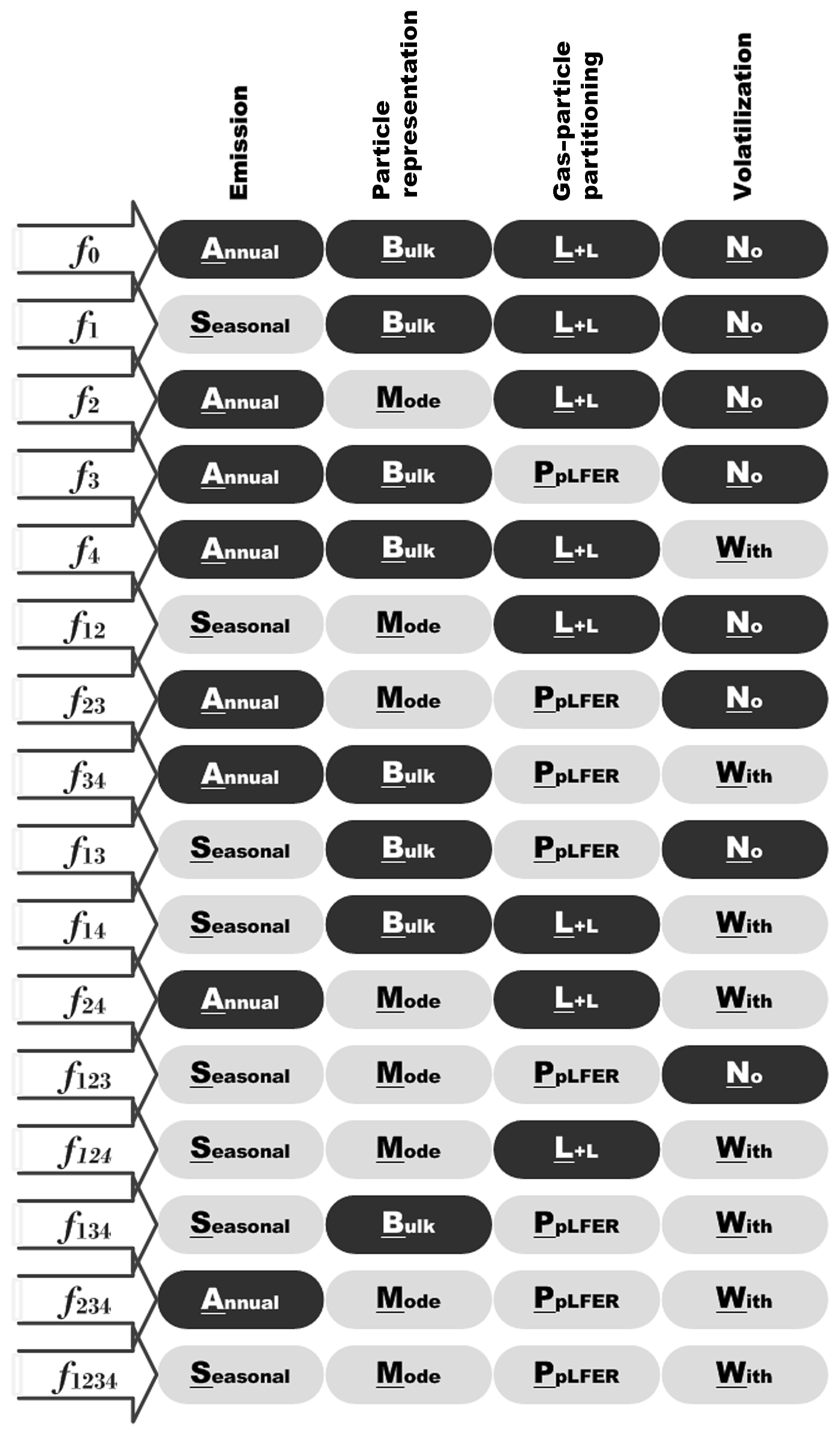
Figure 3List of experiments performed for the factor separation analysis to study sensitivity to temporal variation in emission and process parameterizations (particulate-phase representation, gas–particle partitioning scheme, and volatilization); L+L: Lohmann–Lammel; PpLFER: poly-parameter linear free-energy relationships.
3.1 Sensitivity tests
The analysis of the factor separation results is given below. For each factor, the analysis includes the assessment of direct effects () and total interaction effects () on near-surface PAH concentrations in two seasons, i.e., December–January–February (DJF) and June–July–August (JJA). Figure shows the respective effects for all factors as relative to the seasonal means of the base experiment (f0). A positive value indicates a concentration increase with respect to f0, whereas a negative indicates a decrease. The spatial distributions of f0 and f1234 seasonal mean concentrations for the four species are shown in the Supplement Sect. SVI Figs. S4 and S5, respectively.
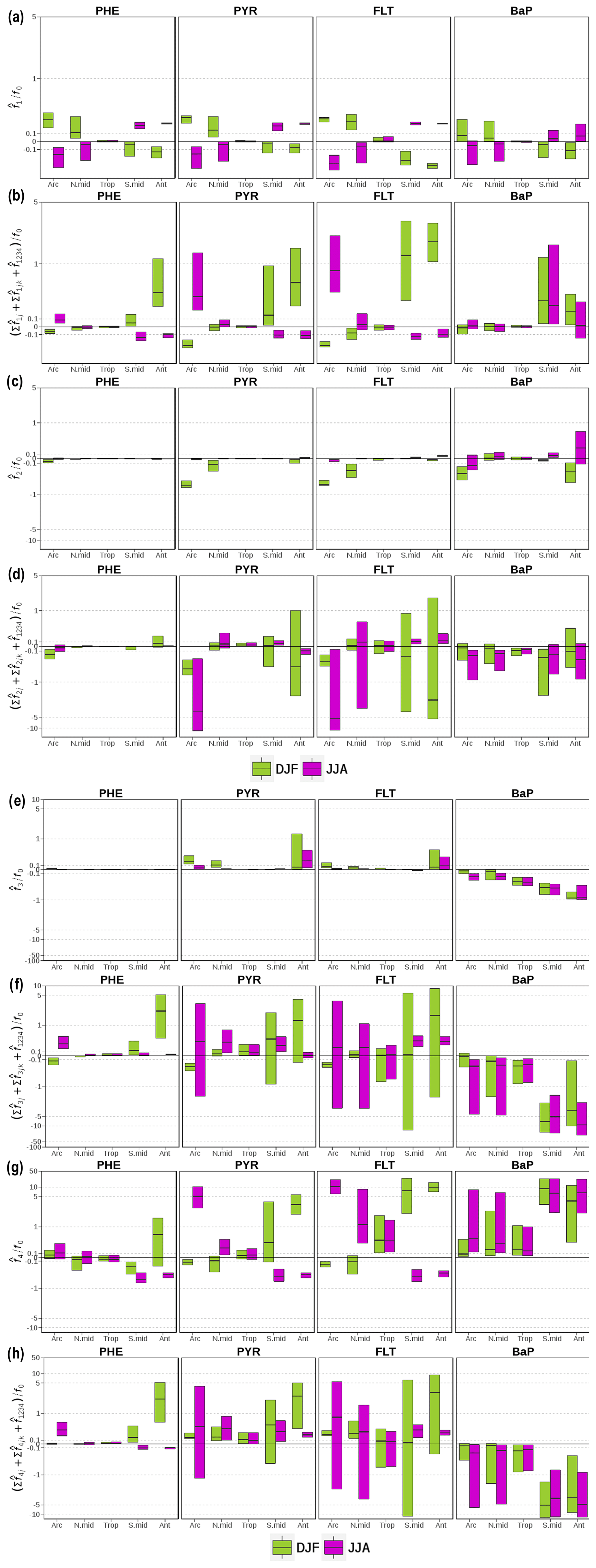
Figure 4Direct and interaction effects on seasonal-mean near-surface PAH concentrations of (a, b) monthly emissions (i=1), (c, d) the modal scheme (i=2), (e, f) the ppLFER scheme (i=3), and (g, h) volatilization (i=4). The direct effects (a, c, e, g) are expressed as the difference between two distributions (), whereas the interaction effects (b, d, f, h) are expressed as the sum of two (, i≠j), three (, ), and all () factor interactions. They are presented as relative to concentrations from the base (f0) simulation. The figures display the median, 25th and 75th percentiles of the relative effects over each of five main climatic regions. Note that an inverse hyperbolic sine function has been used in scaling the y axes.
We studied the relative effects in five climate zones (Arctic, northern midlatitudes, the tropics, southern midlatitudes, and Antarctica) The global distributions of the relative effects are presented in Figs. S6–S13, whereas Figs. S14–S21 present the relative interaction effects from the individual combination of factors. In the following, we do not look to interpret concentration responses to each interaction term. The reasons for this are that (1) accounting for all such interactions is complicated given the number of factors and (2) higher-order interactions (combinations of more than two factors) are hard to physically interpret.
We further investigate the factor effects on model performance by comparing the predicted seasonal mean near-surface concentrations from 16 experiments against observation data in the Arctic and northern midlatitudes (Supplement Sect. SVII).
3.1.1 Effects of seasonality of emissions
Figure a shows that using monthly emissions increases PAH concentrations in DJF and decreases the concentrations in JJA over the areas from the middle to high latitudes of the Northern Hemisphere (NH). This result is expected and is attributed to emissions during the northern winter (summer) being higher (lower) than annual means and photochemistry being less (more) active. Over the Arctic, the relative changes () in DJF show a median increase of approx. 30 % for PHE, PYR, and FLT, and 7 % for BaP, whereas in JJA is weaker in magnitude for PHE and PYR (−16 %) but comparable for FLT (−28 %) and BaP (−5 %). Accounting for seasonality leads to generally lower bias for PHE, and this effect is more pronounced in the middle latitudes rather than in high latitudes (Supplement Sect. SVII, Fig. S22).
In general, becomes smaller over the northern midlatitudes by around half. The upper (lower) quartile of in DJF (JJA) indicates that about one-quarter of the areas of the temperate and polar regions experience an at least 40 % increase (decrease), most were located in northeastern Eurasia (see the left panels of Figs. S6 and S7). Note over the tropics are small to negligible (±1 %) mainly due to little variation in emissions from anthropogenic sectors. PAH concentrations may be higher in dry season due to increased amounts of biomass burning, but they are poorly represented in the current inventory. In southern middle and high latitudes, the direct effects of emission change are substantially opposite in sign to the effects seen in the northern latitudes, being negative in DJF (median ranges from −4 % to −32 %) and positive in JJA (7 %–25 %).
The total interactions between fac1 and other factors generally produce opposite signals to over middle and high latitudes in the two seasons. This result indicates that the changes in other factors tend to buffer the influence of monthly emission on increasing or decreasing f0 concentrations. Some exceptions are seen over parts of East Asia in DJF for all species (Fig. S6, right panels) and over the Southern Ocean in JJA for BaP (Fig. S7, right panels) where the interactions work to reinforce the direct effects. In DJF, the degree of interactions is smaller or comparable to the size of for the Arctic and northern midlatitudes but becomes stronger by at least double for Antarctica. The opposite tendency is seen in JJA but only applies to PYR and FLT. In agreement to , the interaction effects are less apparent over the tropics. Note that the positive effects in during local summer tend to be more dominant than the effects in other combinations for PHE, PYR, and FLT (Figs. S18–S20). In the simulation, the presence of re-volatilization in summer tends to suppress by promoting more gases available for long-range transport, and thus implies a negative feedback.
3.1.2 Effects of size discretization of particulate-phase tracer
The direct effects of the modal scheme () vary among species (Fig. c). is almost absent for PHE as the species resides almost completely in the gas phase. For PYR and FLT, is negative during DJF over northern midlatitudes ( quartiles range from −5 % to −30 %) and the Arctic (−50 % to −75 %), whereas it is hardly visible in JJA or over other regions. Further analysis reveals stronger particle deposition results when the aerosol phase is discretized into different modes (not shown). In long-range transport under modal aerosol representation, the aerosols are more associated with larger particles, hence particle deposition becomes more effective. The choice of size discretization has only minor effects for atmospheric levels, except for BaP, especially during DJF, for which overestimates are significantly compensated for (Fig. S25). Actually, for BaP, the modal scheme generally decreases the concentrations in the Arctic (as median, −35 % in DJF and −15 % during JJA) and increases (approx. 5 %) those over the mid- and low-latitude landmass (Figs. S8d and S9d, left panels).
As is the case for the direct effects, the interaction contributions are peculiar to individual species (Fig. d). For PHE, the interaction effects in DJF are reflected in negative concentration responses over the Arctic (18 %) and positive over Antarctica (7 %), in contrast to relatively mild influences over other regions or in JJA. For PYR and FLT, the effects are negative over the Arctic both in DJF (quartiles vary from −20 % to −75 %) and in JJA (−6 % to −120 %). It is interesting to note that the interaction between the modal and ppLFER schemes has a major influence on the negative signal (Figs. S15, S16, S19, S20), suggesting that the decrease in simulated concentration associated with the change from bulk to modal could be intensified when the ppLFER scheme is used. In the remaining areas, the interaction effects vary in sign spatially as illustrated in the right panels of Figs. S8b and c to S9b and c. Nevertheless, it shows for both species that maximum influences occur over the Southern Ocean in DJF (where the effects may reach 2 orders of magnitude) and midlatitude landmass in JJA (more than a factor of 5). As for BaP, the median effects are negative (−7 % to −30 %) in both seasons, although some positive signals are apparent in parts of high latitudes while the tropical oceans bear small synergistic effects. Similar to other species, the degree of interactions is stronger than by more than a factor of 3 for the majority of grid cells (Figs. S8d–S9d, right panels). The large fractions of the effects are dominated by 2-factor and 3-factor combinations related to the interaction with the ppLFER scheme and/or re-volatilization (Figs. S17, S21).
3.1.3 Effects of the choice of gas–particle partitioning scheme
Figure e shows that the direct effects of the ppLFER scheme () show little spatial heterogeneities in both seasons and for all species. The effects are barely important for PHE due to a low gas–aerosol partition constant (Kp); is positive for PYR and FLT over polar regions and northern midlatitudes especially in winter when low temperature favors partitioning to aerosols (higher Kp). The median of varies from 1 % to 25 % with some parts of Antarctica showing an increase larger than 50 %. For BaP, the effects are overall negative (by at least −5 %) with reflecting a positive north–south gradient (increasing from the Arctic to Antarctica), associated in part with stronger signals over oceans (Figs. S10d and S11d, left panels). In particular under the modal size discretization, the choice of gas–particle partitioning scheme has only minor effects for atmospheric levels, except for BaP for which model overestimates are compensated by the choice of the ppLFER scheme (Fig. S25). Under the bulk size discretization, the ppLFER scheme tends to enhance some of the overestimates in the Arctic summer (FLT, PYR; Figs. S23–S24). The application of ppLFER increases Kp as this module is calculated from not only interaction with BC and OM (as in Lohmann–Lammel scheme) but also with some other aerosol matrices. Higher Kp indicates higher particle mass fraction. For PYR and FLT, this leads to an increase in total atmospheric lifetime as the aerosol phase is not degraded, and can therefore be transported over a larger distance. For BaP, the additional particles are subject to depositions and heterogeneous oxidation by ozone, particularly in regions away from sources. The factor influence is notably too small for PHE as oxidations occur in both phases.
The effects from fac3 interactions vary by region and are relatively stronger than (Fig. f). This finding is common to all species and seasons. The degree of effects is weaker for PHE compared to that for other species. However, the interactions increase polar concentrations in local summer by 20 % to a factor of 5, mainly associated with the coupled effect of ppLFER and volatilization (, Figs. S14 and S18). For PYR and FLT, there is a high spatial variability over extratropical regions in local summer, as indicated by the interquartile range (distance between the third and first quartiles). With regard to synergistic terms, ppLFER interactions with the modal scheme and re-volatilization, in 2- or 3-factor combinations, are more important than other contributions (Figs. S15–S16 and S19–S20). For BaP, the interaction effects show negative signals similar to , suggesting a positive feedback. The interactions exert a stronger influence on the concentrations of the oceans than on that of land, except in the tropics (Figs. S10d and S11d, right panels). The median of relative effects ranges from −1 % to a factor of −10, minimum (maximum) in the northern (southern) extratropics. Two second-order interactions likely make major contributions, i.e., which dominates the response over oceans and which dominates over land (Figs. S17 and S21).
3.1.4 Effects of re-volatilization
The direct effects of re-volatilization () are illustrated in Fig. g. is positive in the tropics in both seasons, with the median ranging from 5 % to 50 %. Intensive re-volatilization in this region would increase net surface fluxes, thereby increasing concentrations. For PHE, positive values are more localized over the tropical landmass, whereas negative values are predicted over the tropical ocean (Figs. S12a and S13a; left panels). The positive (negative) effects over land (ocean) areas are also apparent at higher latitudes during most of the year. This reflects the fact that the negative effects on concentrations over ocean act contrary to the positive effects on net surface fluxes, mainly caused by the nonlinear relationships of air–sea gas exchange (deposition and volatilization), air and surface burden, atmospheric oxidation, and emissions. Accounting for re-volatilization compensates for a significant part of underestimates of PHE in the Arctic during summer, but adds to overestimates in midlatitudes (Fig. S22).
For the studied species of mid semivolatility, PYR and FLT, a positive signal is apparent over the high and middle latitudes during local summer in contrast to a negative signal during local winter (Fig. g). Similar to PHE, the negative signal is confined over oceans (Figs. S12b–c and S13b–c; left panels). The summer increases are stronger (20 % to a factor of 10) than the winter decreases (−10 % to −60 %) and the magnitudes are higher in FLT than in PYR. The near-ground concentrations of PYR and FLT are estimated to be ≈30 %–80 % in midlatitudes of which ≈30 % are attributable to re-volatilization. In the Arctic, re-volatilization compensates for ≈60 % of PYR underestimation (Fig. S23) and explains most of, ≈60 %–80 %, the FLT overestimation (Fig. S24). For BaP, is positive consistently across regions and seasons ( ranges from 20 % to a factor of 10), with substantial effects occurring over oceans (Figs. S12d–S13d; left panels). Accounting for re-volatilization creates some overestimates in the Arctic during summer (Fig. S25). It should be noted that the parameterization adopted here to describe volatilization from soils (the Smit scheme) is derived from an experimental study on mid-polar-to-polar pesticides and there is a need to validate and eventually sophisticate the parameterization to apolar substances.
The interactions generally point toward positive effects for the high-to-medium volatility species (Fig. h), despite some negative effects present over parts of the southern (northern) oceans in DJF (JJA) (Figs. S12–S13; right panels). As for BaP, the effects are uniformly negative, inferring the interactions work in opposition to . The negative response is almost entirely caused by the negative , i.e., the 2-factor interaction between re-volatilization and the ppLFER scheme (Figs. S17, S21). Compared to , the degree of interactions is weaker for PHE, except in polar regions during local summer where the interactions could amplify . The above implies that may point in the right direction regardless of the influences from other factor changes. In contrast, the degree of interactions is overall comparable to for the other species.
3.2 Model evaluation
Model performance using the sophisticated realization of the four features (factors), i.e., Seasonal emission + Modal scheme + PpLFER scheme + With re-volatilization (SMPW), is presented below. Two predicted variables are evaluated, i.e., total (gas+particle) concentrations and aerosol particulate mass fraction at the lowest model level. The metrics applied are listed in the Supplement Sect. SV.

Figure 5Seasonal mean total (gas+particle) concentrations of PAHs (ng m−3) from observations (solid lines) and simulations (dashed lines) averaged over all stations in the (a) Arctic, (b) northern midlatitudes, and (c) the tropics. Note that a logarithmic scale has been used for BaP concentrations in the Arctic.
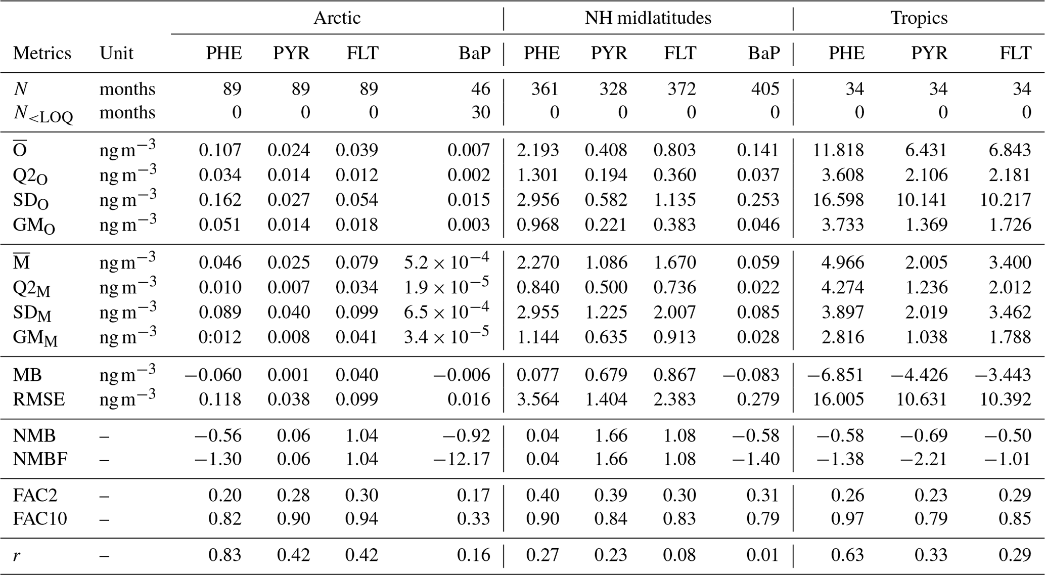
Table 2Statistics comparison of model simulation and observations of total (gas+particle) concentrations of PAHs from stations in the Arctic, northern midlatitudes, and the tropics. N: Number of observed-simulated monthly data pairs; : mean; Q2x: median; SDx: standard deviation; GMx: geometric mean; x: simulated (M) or observed (O) data; MB: mean bias; RMSE: root mean square error; NMB: normalized mean bias; NMBF: normalized mean bias factor; FAC2: factor of 2; FAC10: factor of 10; r: correlation coefficient.
3.2.1 Near-surface air concentration
Firstly, the comparison to land monitoring stations is as follows.
-
Central tendency. Table 2 shows statistical indices for near-surface concentrations of atmospheric PAHs from observations and simulations and their comparisons, averaged across stations in the Arctic, northern midlatitudes, and the tropics. We can see that observed mean concentrations are higher for PHE and smaller for BaP over all regions. Furthermore, the Arctic concentrations are lower than those in the northern midlatitudes by a factor of around 20 and those in the tropics by approx. 2 orders of magnitude. The model captures well these species and regional variations, but the magnitudes are both underestimated and overestimated. In the Arctic, it underestimates PHE (MB ng m−3) and BaP (MB ng m−3) concentrations but slightly overestimates PYR (MB =0.001 ng m−3) and FLT (MB =0.04 ng m−3). In the NH midlatitudes, the model overestimates the three species predominantly occurring in the gas phase (MB =0.077–0.867 ng m−3) but underestimates BaP (MB ng m−3). Negative bias is seen in the tropics for three PAHs (MB to −6.851 ng m−3). Nevertheless, the comparison of model and observations at individual monitoring stations can be different from the regional mean statistics, as described in the Supplement Sect. SVIII. Comparing all four PAHs, a larger degree of bias is found for BaP, which increases from the northern midlatitudes (NMB , NMBF , FAC2 =0.31, FAC10 =0.79) to the Arctic (NMB , NMBF , FAC2 =0.17, FAC10 =0.33).
-
Dispersion of monthly concentrations. In the following, the coefficient of variation (CoV) is used to compare the dispersion of concentrations among species of different ranges. CoV was calculated by dividing the standard deviation (SD) of all data points by its mean value (). The observations show high variability (CoV >1) with CoV ranging between 1.12 and 2.14. The simulated concentrations appear to be less dispersed than the observations (CoV =0.78–1.93) except for the Arctic PHE and PYR concentrations. The degree of underestimation is larger in the tropics with CoV being 30 %–50 % smaller than the observations. Furthermore, correlations between predicted and observed concentrations are weaker than those in other regions where r varies between 0.29 and 0.63 (the model reproduces 8 %–40 % of the variance in observed concentrations). Comparing the four species, the simulated BaP shows greater underpredictions of the variability where CoV values are less than half of those observed and correlations are less than 0.2 (accounting not over 4 % of observed variance). Higher variability in BaP measurements (than in model results) can be influenced by strongly varying emissions in source regions that are not reflected in the emission inventory (Matthias et al., 2009).
-
Seasonal variation. Figure compares simulated and observed seasonal cycle of average concentrations for different species and regions. The observed mean concentrations are largest in winter and lowest during summer because of less emission and the strong presence of OH for oxidation. The winter maximum to summer minimum ratio (amplitude) is more pronounced (by more than a factor of 2) in the Arctic than that in the NH midlatitudes. The seasonality between model and observations is in qualitative agreement, particularly over the Arctic (except in summer) and midlatitudes. In the Arctic, the model overestimates the seasonal amplitude of PHE and BaP and underestimates their mean concentrations. The contrast is seen for PYR and FLT. FLT concentration is overestimated by up to a factor of 3 in summer while PYR is quite well predicted. In the NH midlatitudes, the model underestimates the amplitude but overestimates the concentrations of PHE, PYR, and FLT (by typically a factor of 2), whereas a systematic negative bias is found for BaP. In the tropics, both the amplitude and magnitude are too low in the model (for magnitude, by a factor of 2–5).
Additional findings are discussed in the Supplement Sect. SIX related to the comparison between EMAC model results and those from other global PAH modeling studies.
Secondly, the comparison to ship cruise measurements is as follows. Measurements of PHE, PYR, and FLT concentrations over the Atlantic Ocean were taken during a cruise in July 2009 (Lohmann et al., 2013). Figure 5 shows the ship sample concentrations overlaying the simulated PAH concentrations. Sample arithmetic (geometric) means during the whole cruise transect are 322 (209), 95 (88), and 128 (111) pg m−3 for PHE, PYR, and FLT, respectively. The model poorly reproduces the remote marine environments and overall underestimates the observations, except at 3 locations along the North American coast. The simulated means across sampling positions are 23 (7), 20 (3), and 39 (2) pg m−3, respectively, and the underestimation ranges from a factor of 2 to 1000. The degree of bias is most apparent over the tropical South Atlantic at latitude band 5–15∘ S.
As reported in Liu et al. (2014), the measured concentrations of BaP over the Asian marginal seas, the Indian Ocean, the South Pacific Ocean, and North Pacific Ocean are 131 (45), 14 (3), 9 (2), and 8 (3) pg m−3, respectively, for the arithmetic (geometric) means of all samples. Similar to other species, the model also underestimates the BaP concentrations with mean values being 75 (15), 4 (0.05), 0.09 (0.03), and 0.2 (0.06) pg m−3, respectively. The discrepancy appears relatively smaller over the Asian marginal seas as compared to other locations (Fig. 6). A substantial degree of bias is seen over the Indian Ocean covering approximately the area bounded by 70–90∘ E and 10–30∘ S, with simulated values being more than 2 orders of magnitude smaller than the observed.
The model tendency to underestimate the marine air concentrations may likely be due to several factors. (a) The grid resolution is not sufficient to reproduce fine-scale processes at the grid points close to shipping tracks; (b) high uncertainties associated with the air–sea gas exchange parameterizations still exist, most notably in the estimation of gas transfer velocity; (c) the global inventory (Shen et al., 2013) may significantly underestimate emissions from ocean shipping and does not well characterize the spatial and temporal variability of biomass burning plumes as another potential point of origin of pollutants in the marine air (Nizzetto et al., 2008); and (d) PAH concentration over remote oceans is controlled by atmospheric components (e.g., temperature, wind speed, boundary layer height, photochemical degradation) and the dynamical and biogeochemical components of the ocean. However, the ocean components have not been covered in the simulation; (e) the particulate-bound PAHs may undergo too fast heterogeneous oxidation (most relevant for BaP), leading to short atmospheric lifetimes and weaker long-range transport. BaP, mostly stays in the particulate phase, presumably also in seawater, and therefore may be somewhat underestimated due to the neglect of sea-spray-driven aerosol suspension.
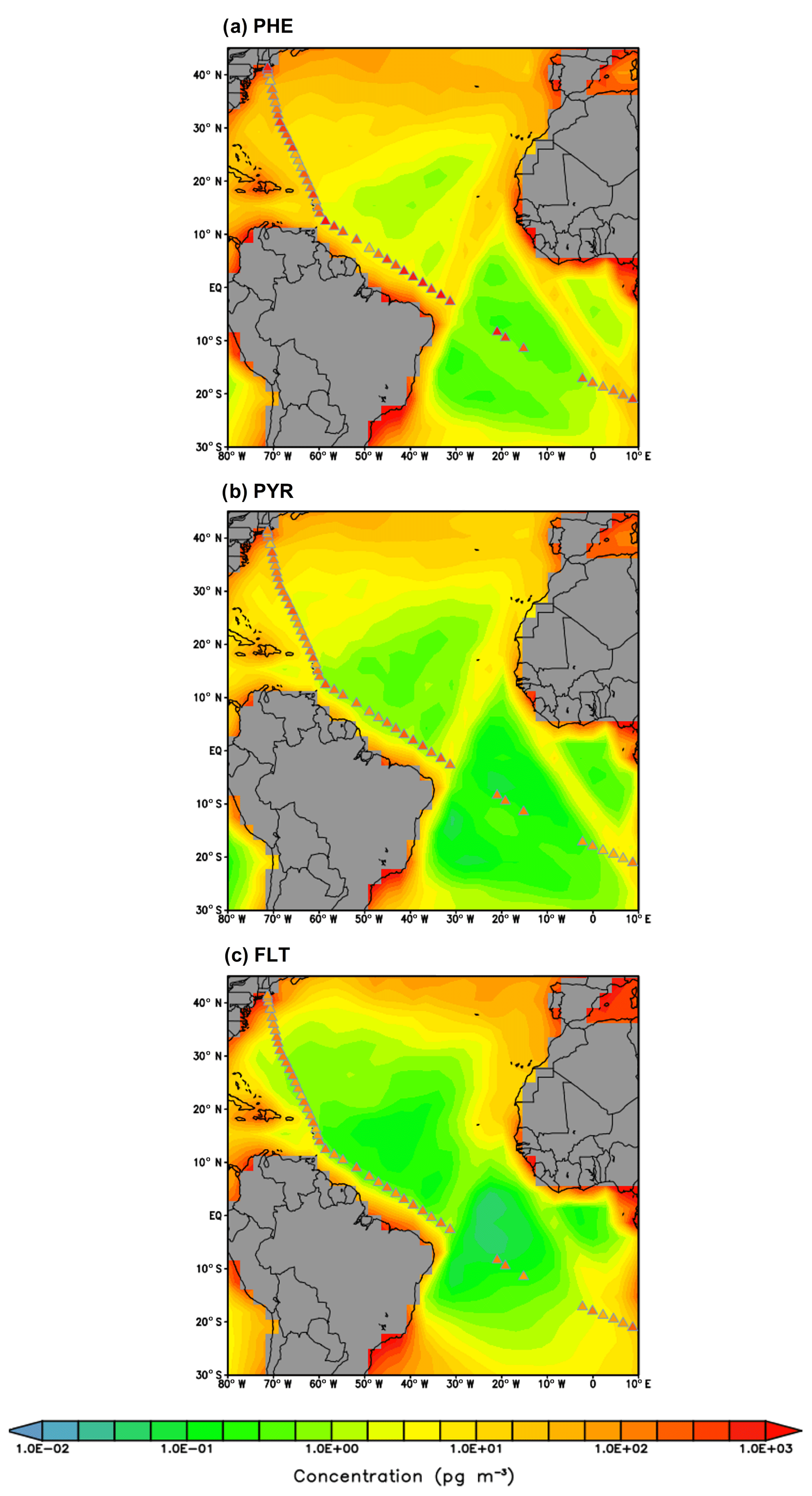
Figure 6Simulated concentrations of PHE, PYR, and FLT (pg m−3) over the Atlantic ocean overlaid with concentrations from a ship cruise measurement campaign during July 2009 (triangles). Land grid cells are depicted in gray shades.

Figure 7Simulated BaP concentrations (pg m−3) over the four ocean margins overlaid with concentrations from a ship cruise measurement campaign (triangles). Land grid cells are depicted in gray shades.
3.2.2 Particulate mass fraction
Measurements of particulate mass fraction (θ) were available only from the E3 station in Europe and IADN stations (I1–I7) in North America (see Table S11). Table 3 presents summary statistics on monthly mean θ from observations and simulations including some performance metrics. The observed mean θ is smaller for PHE (0.051±0.035) and higher for BaP (0.949±0.067). This result is expected as volatility decreases (hence θ increases) from (lighter) PHE to (heavier) BaP. The θ values for PYR and FLT are larger by over 5 times than those for PHE and lower by around one-third than those for BaP. The model reproduces well the distinct differences among species but underestimates the observed θ for PHE, PYR, and FLT. The degree of negative bias is relatively large in PHE (NMB and NMBF ), whereas for the isomer pair of PYR and FLT, the model exhibits a similar performance with a slight improvement in PYR (NMB and NMBF ). With regard to BaP, there is a satisfactorily small bias (MB =0.015, RMSE =0.074, NMB =0.016, and NMBF =0.016) although the observed and simulated values have a very weak correlation (r=0.03).
Table 3Statistics comparison of model simulation and observations of particulate mass fraction (θ) from a subset of surface stations, as listed in Table S11. N: Number of observed-simulated monthly data pairs; : mean; SDx: standard deviation; x: simulated (M) or observed (O) data; MB: mean bias; RMSE: root mean square error; NMB: normalized mean bias; NMBF: normalized mean bias factor; FAC2: factor of 2; FAC10: factor of 10; r: correlation coefficient.
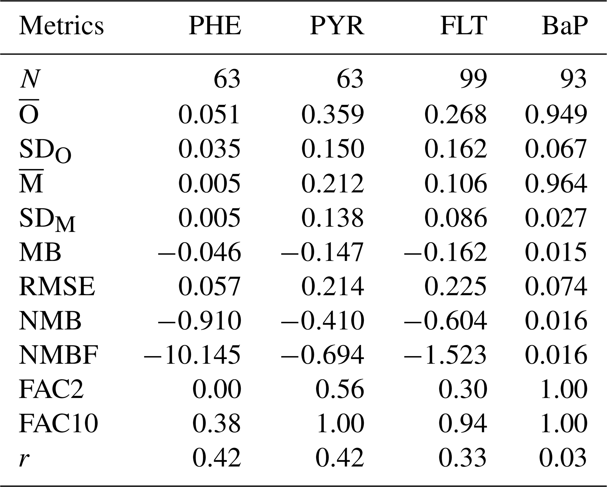
Figure 7 shows the seasonal mean θ averaged over 3 years for all PAHs. Observations show that θ for BaP varies less than those for 3–4-ring PAHs. Although the model adequately reproduces this feature as well as seasonal variation of individual species, the simulated θ of PHE, PYR, and FLT is generally lower than the observations (except for PYR in winter). For BaP, differences between model and observations are less than 10 % in all months. The SVOC submodel describes the gas–particle partitioning of atmospheric SOCs as a function of temperature and aerosol phase composition. The underestimation might be related to the fact that the submodel assumes the particle to be fully in equilibrium with the gas phase at all times. It neglects kinetic limitations of molecular diffusivity that could lead to the trapping of particles inside viscous (or semisolid) organic aerosol coatings. This shielding effect increases equilibration times of the particles, thereby reducing part of θ from the mass available for gas–particle partitioning. Deviations from measurements can also be partly attributed to the locations of some stations that are within, or close to, residential and industrial area (namely I4, I6, and I7) where the scale and gradient in anthropogenic emissions are not resolved by the model grid resolution nor represented by the emission inventory.
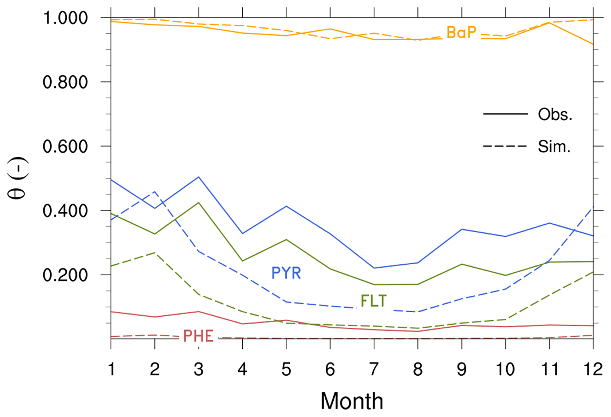
Figure 8Seasonal mean particulate mass fraction (θ; unitless) from observations (solid lines) and simulations (dashed lines).
The submodel SVOC has been developed and operated within the EMAC model for the application to global distribution and environmental fate of SOCs. In this first development, the focus was set on the predictions of four PAH species: phenanthrene (PHE), pyrene (PYR), fluoranthene (FLT), and benzo(a)pyrene (BaP). Multicompartmental fate and air–surface exchange processes were included in SVOC. Some novel features in PAH modeling were tested, including seasonality in emissions, the modal scheme for particulate-phase tracer representation, the ppLFER scheme for gas–particle partitioning, and re-volatilization from surfaces. The results indicate that using seasonal emission compensates for model biases in the predictions of more volatile species (PHE), whereas the effects of the modal and ppLFER schemes are of less significance. Re-volatilization increases the near-ground concentrations in air, which is found most significant for species of mid semivolatility (PYR and FLT). The attribution of model response to individual features (factors) is blurred by the nonlinear interactions between two or more factors. The effects of these interactions are found to both reinforce (positive feedback) and suppress (hence negative feedback) the effects of the individual factors.
For near-surface concentrations, model bias varies by region and/or species, being negative (positive) in the Arctic within typically a factor of 2–13 (6 % to a factor of 2) for PHE and BaP (PYR and FLT); positive in the northern midlatitudes for PHE, PYR, and FLT by up to a factor of 3; negative in the tropics (by a factor of 2–3); and largely over ocean up to 3 orders of magnitude. The model adequately reproduces the seasonal variation of the particulate mass fraction (θ), but underestimates θ for high-to-medium-volatility PAHs. This might be related to a systematic underestimation of OC by the model, which neglects secondary organic aerosols (SOA). The latter may cause significant underestimation of the overall atmospheric aerosol burden and θ of SOCs, in particular over ocean. Since recently a MESSy submodel, ORACLE, dedicated to the simulations of SOA (Tsimpidi et al., 2014) based on lumping organic species in volatility bins is available. It should be included in future SOC simulations using EMAC.
Moreover, the implicit assumption of instantaneous gas–particle equilibrium for SVOC may cause both over- and underestimates of θ, as interphase mass transfer my be kinetically limited to gaseous sources (hence overestimate of θ) or within the particle bulk (hence underestimate θ), as the PAHs may become trapped within particles during transport (Friedman et al., 2014; Zelenyuk et al., 2012; Mu et al., 2018). For multidecadal studies, the coupling of a 3-D ocean model (coupled with a marine biogeochemistry module) would be needed since the present model application does not allow for horizontal and vertical transports in the deep ocean. For the same reason, contaminant remobilization within deep soil layers should also be introduced. To this end, a multilayer (3-D) soil compartment would be needed to replace the 2-D soil compartment used here.
The SVOC submodel presented here is based on the Modular Earth Submodel System (MESSy) version 2.50 and the global atmospheric model ECHAM version 5.3.02. MESSy is continuously developed and applied by a consortium of institutions. The usage of MESSy and access to the source code is licensed to all affiliates of institutions which are members of the MESSy Consortium. Institutions can be a member of the MESSy Consortium by signing the MESSy Memorandum of Understanding. More information can be found at http://www.messy-interface.org (MESSy Consortium, 2018). The SVOC submodel will be incorporated into the next release version of the ECHAM/MESSy (EMAC) model (v2.55) and will therefore be made publicly available (with respect to the EMAC license regulations).
The supplement related to this article is available online at: https://doi.org/10.5194/gmd-12-3585-2019-supplement.
MO and GL conceived the study and designed the experiments. MO developed the SVOC submodel with input from all co-authors. MO performed model simulations and data analyses. MO and GL discussed the results. MO wrote the article with contributions from all co-authors.
The authors declare that they have no conflict of interest.
This study was supported by the Max Planck Institute for Chemistry. We thank the MESSy community and MESSy submodel developers for providing technical support. The model simulation was performed at the Max Planck Computing and Data Facility (MPCDF), Garching.
The article processing charges for this open-access publication were covered by the Max Planck Society.
This paper was edited by Havala Pye and reviewed by two anonymous referees.
Batjes, N.: Total carbon and nitrogen in the soils of the world, Eur. J. Soil Sci., 47, 151–163, https://doi.org/10.1111/j.1365-2389.1996.tb01386.x, 1996. a
Dalla Valle, M., Codato, E., and Marcomini, A.: Climate change influence on POPs distribution and fate: A case study, Chemosphere, 67, 1287–1295, https://doi.org/10.1016/j.chemosphere.2006.12.028, 2007. a
Daly, G. L. and Wania, F.: Simulating the influence of snow on the fate of organic compounds, Environ. Sci. Technol., 38, 4176–4186, https://doi.org/10.1021/es035105r, 2004. a
de Boyer Montégut, C., Madec, G., Fischer, A. S., Lazar, A., and Iudicone, D.: Mixed layer depth over the global ocean: An examination of profile data and a profile-based climatology, J. Geophys. Res.-Oceans, 109, C12003, https://doi.org/10.1029/2004JC002378, 2004. a
Dee, D. P., Uppala, S. M., Simmons, A. J., Berrisford, P., Poli, P., Kobayashi, S., Andrae, U., Balmaseda, M. A., Balsamo, G., Bauer, P., Bechtold, P., Beljaars, A. C. M., van de Berg, L., Bidlot, J., Bormann, N., Delsol, C., Dragani, R., Fuentes, M., Geer, A. J., Haimberger, L., Healy, S. B., Hersbach, H., Hólm, E. V., Isaksen, L., Kållberg, P., Köhler, M., Matricardi, M., McNally, A. P., Monge-Sanz, B. M., Morcrette, J.-J., Park, B.-K., Peubey, C., de Rosnay, P., Tavolato, C., Thépaut, J.-N., and Vitart, F.: The ERA−Interim reanalysis: configuration and performance of the data assimilation system, Q. J. Roy. Meteor. Soc., 137, 553–597, https://doi.org/10.1002/qj.828, 2011. a
DEFRA: UK Department of Environment, Food and Rural Affairs, Polycyclic Aromatic Hydrocarbons (PAH) data, available at: https://uk-air.defra.gov.uk/data/pah-data (last access: 15 August 2017), 2010. a
Dunne, K. A. and Willmott, C. J.: Global distribution of plant-extractable water capacity of soil, Int. J. Climatol., 16, 841–859, https://doi.org/10.1002/(SICI)1097-0088(199608)16:8<841::AID-JOC60>3.0.CO;2-8, 1996. a
Endo, S. and Goss, K.-U.: Applications of polyparameter linear free energy relationships in environmental chemistry, Environ. Sci. Technol., 48, 12477–12491, https://doi.org/10.1021/es503369t, 2014. a, b
European Commission: Guidance document on persistence in soil, Technical Report 9188/VI/97 in relation to Council Directive No. 97/57/EC, EC Directorate General for Agriculture, 2000. a
Finizio, A., Mackay, D., Bidleman, T., and Harner, T.: Octanol−air partition coefficient as a predictor of partitioning of semi-volatile organic chemicals to aerosols, Atmos. Environ., 31, 2289–2296, https://doi.org/10.1016/S1352-2310(97)00013-7, 1997. a
Friedman, C. L. and Selin, N. E.: Long-range atmospheric transport of polycyclic aromatic hydrocarbons: global 3-D model analysis including evaluation of Arctic sources, Environ. Sci. Technol., 46, 9501–9510, https://doi.org/10.1021/es301904d, 2012. a, b, c
Friedman, C. L., Pierce, J. R., and Selin, N. E.: Assessing the influence of secondary organic versus primary carbonaceous aerosols on long-range atmospheric polycyclic aromatic hydrocarbon transport, Environ. Sci. Technol., 48, 3293–3302, https://doi.org/10.1021/es405219r, 2014. a
Galarneau, E., Makar, P. A., Zheng, Q., Narayan, J., Zhang, J., Moran, M. D., Bari, M. A., Pathela, S., Chen, A., and Chlumsky, R.: PAH concentrations simulated with the AURAMS-PAH chemical transport model over Canada and the USA, Atmos. Chem. Phys., 14, 4065–4077, https://doi.org/10.5194/acp-14-4065-2014, 2014. a, b
Gantt, B., Meskhidze, N., Facchini, M. C., Rinaldi, M., Ceburnis, D., and O'Dowd, C. D.: Wind speed dependent size-resolved parameterization for the organic mass fraction of sea spray aerosol, Atmos. Chem. Phys., 11, 8777–8790, https://doi.org/10.5194/acp-11-8777-2011, 2011. a
Gong, S. L., Huang, P., Zhao, T. L., Sahsuvar, L., Barrie, L. A., Kaminski, J. W., Li, Y. F., and Niu, T.: GEM/POPs: a global 3-D dynamic model for semi-volatile persistent organic pollutants – Part 1: Model description and evaluations of air concentrations, Atmos. Chem. Phys., 7, 4001–4013, https://doi.org/10.5194/acp-7-4001-2007, 2007. a
Goss, K.-U. and Schwarzenbach, R. P.: Linear free energy relationships used to evaluate equilibrium partitioning of organic compounds, Environ. Sci. Technol., 35, 1–9, https://doi.org/10.1021/es000996d, 2001. a, b
Guelle, W., Schulz, M., Balkanski, Y., and Dentener, F.: Influence of the source formulation on modeling the atmospheric global distribution of sea salt aerosol, J. Geophys. Res.-Atmos., 106, 27509–27524, https://doi.org/10.1029/2001JD900249, 2001. a
Gullett, B., Touati, A., and Oudejans, L.: PCDD/F and aromatic emissions from simulated forest and grassland fires, Atmos. Environ., 42, 7997–8006, https://doi.org/10.1016/j.atmosenv.2008.06.046, 2008. a
Gusev, A., Mantseva, E., Shatalov, V., and B., S.: Regional Multicompartment Model MSCE-POP, EMEP/MSC-E Technical Report 5, 2005. a
Hansen, K. M., Christensen, J. H., Brandt, J., Frohn, L. M., and Geels, C.: Modelling atmospheric transport of α-hexachlorocyclohexane in the Northern Hemispherewith a 3-D dynamical model: DEHM-POP, Atmos. Chem. Phys., 4, 1125–1137, https://doi.org/10.5194/acp-4-1125-2004, 2004. a
Hung, H., Blanchard, P., Halsall, C. J., Bidleman, T. F., Stern, G. A., Fellin, P., Muir, D. C. G., Barrie, L. A., Jantunen, L. M., Helm, P. A., Ma, J., and Konoplev, A.: Temporal and spatial variabilities of atmospheric polychlorinated biphenyls (PCBs), organochlorine (OC) pesticides and polycyclic aromatic hydrocarbons (PAHs) in the Canadian Arctic: Results from a decade of monitoring, Sci. Total Environ., 342, 119–144, https://doi.org/10.1016/j.scitotenv.2004.12.058, 2005. a
IADN: Great Lakes Integrated Atmospheric Deposition Network, available at: http://ec.gc.ca/data_donnees/STB-AQRD/Toxics/IADN (last access: 7 November 2017), 2014. a
Janssens-Maenhout, G., Crippa, M., Guizzardi, D., Dentener, F., Muntean, M., Pouliot, G., Keating, T., Zhang, Q., Kurokawa, J., Wankmüller, R., Denier van der Gon, H., Kuenen, J. J. P., Klimont, Z., Frost, G., Darras, S., Koffi, B., and Li, M.: HTAP_v2.2: a mosaic of regional and global emission grid maps for 2008 and 2010 to study hemispheric transport of air pollution, Atmos. Chem. Phys., 15, 11411–11432, https://doi.org/10.5194/acp-15-11411-2015, 2015. a
Jöckel, P., Tost, H., Pozzer, A., Brühl, C., Buchholz, J., Ganzeveld, L., Hoor, P., Kerkweg, A., Lawrence, M. G., Sander, R., Steil, B., Stiller, G., Tanarhte, M., Taraborrelli, D., van Aardenne, J., and Lelieveld, J.: The atmospheric chemistry general circulation model ECHAM5/MESSy1: consistent simulation of ozone from the surface to the mesosphere, Atmos. Chem. Phys., 6, 5067–5104, https://doi.org/10.5194/acp-6-5067-2006, 2006. a, b, c, d, e
Jöckel, P., Kerkweg, A., Pozzer, A., Sander, R., Tost, H., Riede, H., Baumgaertner, A., Gromov, S., and Kern, B.: Development cycle 2 of the Modular Earth Submodel System (MESSy2), Geosci. Model Dev., 3, 717–752, https://doi.org/10.5194/gmd-3-717-2010, 2010. a, b, c
Junge, C.: Basic considerations about trace constituents in the atmosphere as related to the fate of global pollutants, John Wiley & Sons, New York, 7–26, 1977. a
Jury, W. A., Spencer, W. F., and Farmer, W. J.: Behavior assessment model for trace organics in soil: I. Model description, J. Environ. Qual., 12, 558–564, https://doi.org/10.2134/jeq1983.00472425001200040025x, 1983. a
Jury, W. A., Russo, D., Streile, G., and el Abd, H.: Evaluation of volatilization by organic chemicals residing below the soil surface, Water Resour. Res., 26, 13–20, https://doi.org/10.1029/WR026i001p00013, 1990. a
Kerkweg, A., Buchholz, J., Ganzeveld, L., Pozzer, A., Tost, H., and Jöckel, P.: Technical Note: An implementation of the dry removal processes DRY DEPosition and SEDImentation in the Modular Earth Submodel System (MESSy), Atmos. Chem. Phys., 6, 4617–4632, https://doi.org/10.5194/acp-6-4617-2006, 2006a. a, b, c
Kerkweg, A., Sander, R., Tost, H., and Jöckel, P.: Technical note: Implementation of prescribed (OFFLEM), calculated (ONLEM), and pseudo-emissions (TNUDGE) of chemical species in the Modular Earth Submodel System (MESSy), Atmos. Chem. Phys., 6, 3603–3609, https://doi.org/10.5194/acp-6-3603-2006, 2006b. a, b, c
Klánová, J., Cupr, P., Holoubek, I., Boruvková, J., Přibylová, P., Kareš, R., Kohoutek, J., Dvorská, A., Tomšej, T., and Ocelka, T.: Application of passive sampler for monitoring of POPs in ambient air. VI. Pilot study for development of the monitoring network in the African continent (MONET-AFRICA 2008), RECETOX_TOCOEN 343, RECETOX MU Brno, Czech Republic, 2008. a
Kwamena, N.-O. A., Thornton, J. A., and Abbatt, J. P. D.: Kinetics of surface-bound benzo[a]pyrene and ozone on solid organic and salt aerosols, J. Phys. Chem. A, 108, 11 626–11 634, https://doi.org/10.1021/jp046161x, 2004. a
Laender, F. D., Hammer, J., Hendriks, A. J., Soetaert, K., and Janssen, C. R.: Combining monitoring data and modeling identifies PAHs as emerging contaminants in the Arctic, Environ. Sci. Technol., 45, 9024–9029, https://doi.org/10.1021/es202423f, 2011. a
Lammel, G.: Polycyclic aromatic compounds in the atmosphere – A review identifying research needs, Polycycl. Aromat. Comp., 35, 316–329, https://doi.org/10.1080/10406638.2014.931870, 2015. a
Lammel, G., Klánová, J., Ilić, P., Kohoutek, J., Gasić, B., Kovacić, I., and Škrdlíková, L.: Polycyclic aromatic hydrocarbons in air on small spatial and temporal scales – II. Mass size distributions and gas–particle partitioning, Atmos. Environ., 44, 5022–5027, https://doi.org/10.1016/j.atmosenv.2010.08.001, 2010. a
Lamon, L., Dalla Valle, M., Critto, A., and Marcomini, A.: Introducing an integrated climate change perspective in POPs modelling, monitoring and regulation, Environ. Pollut., 157, 1971–1980, https://doi.org/10.1016/j.envpol.2009.02.016, 2009. a
Landgraf, J. and Crutzen, P. J.: An efficient method for online calculations of photolysis and heating rates, J. Atmos. Sci., 55, 863–878, https://doi.org/10.1175/1520-0469(1998)055<0863:AEMFOC>2.0.CO;2, 1998. a
Lauer, A., Eyring, V., Hendricks, J., Jöckel, P., and Lohmann, U.: Global model simulations of the impact of ocean-going ships on aerosols, clouds, and the radiation budget, Atmos. Chem. Phys., 7, 5061–5079, https://doi.org/10.5194/acp-7-5061-2007, 2007. a
Liss, P. S. and Slater, P. G.: Flux of gases across the air–sea interface, Nature, 247, 181–184, https://doi.org/10.1038/247181a0, 1974. a
Liu, J., Xu, Y., Li, J., Liu, D., Tian, C., Chaemfa, C., and Zhang, G.: The distribution and origin of PAHs over the Asian marginal seas, the Indian, and the Pacific Oceans: Implications for outflows from Asia and Africa, J. Geophys. Res.-Atmos., 119, 1949–1961, https://doi.org/10.1002/2013JD020361, 2014. a, b
Lohmann, R. and Lammel, G.: Adsorptive and absorptive contributions to the gas−particle partitioning of polycyclic aromatic hydrocarbons: State of knowledge and recommended parametrization for modeling, Environ. Sci. Technol., 38, 3793–3803, https://doi.org/10.1021/es035337q, 2004. a, b
Lohmann, R., Klánová, J., Příbylová, P., Lišková, H., Yonis, S., and Bollinger, K.: PAHs on a west-to-east transect across the tropical Atlantic Ocean, Environ. Sci. Technol., 47, 2570–2578, https://doi.org/10.1021/es304764e, 2013. a, b
Ma, J., Daggupaty, S., Harner, T., and Li, Y.: Impacts of lindane usage in the Canadian prairies on the Great Lakes ecosystem. 1. Coupled atmospheric transport model and modeled concentrations in air and soil, Environ. Sci. Technol., 37, 3774–3781, https://doi.org/10.1021/es034160x, 2003. a
Mackay, D.: Multimedia environmental models: The fugacity approach, 2nd Edn., Taylor & Francis, available at: http://books.google.de/books?id=f37zywrLJf0C (last access: 26 April 2018), 2010. a
Mackay, D. and Boethling, R. S.: Handbook of property estimation methods for chemicals: Environmental health sciences, Taylor & Francis, available at: https://books.google.de/books?id=EhHutGUI3zwC (last access: 26 April 2018), 2000. a
MacLeod, M., Riley, W. J., and McKone, T. E.: Assessing the influence of climate variability on atmospheric concentrations of polychlorinated biphenyls using a global-scale mass balance model (BETR-global), Environ. Sci. Technol., 39, 6749–6756, https://doi.org/10.1021/es048426r, 2005. a
MacLeod, M., von Waldow, H., Tay, P., Armitage, J. M., Wöhrnschimmel, H., Riley, W. J., McKone, T. E., and Hungerbuhler, K.: BETR global − A geographically-explicit global-scale multimedia contaminant fate model, Environ. Pollut., 159, 1442–1445, https://doi.org/10.1016/j.envpol.2011.01.038, 2011. a
Malanichev, A., Mantseva, E., Shatalov, V., Strukov, B., and Vulykh, N.: Numerical evaluation of the PCBs transport over the Northern Hemisphere, Environ. Pollut., 128, 279–289, https://doi.org/10.1016/j.envpol.2003.08.040, 2004. a
Matthias, V., Aulinger, A., and Quante, M.: CMAQ simulations of the benzo(a)pyrene distribution over Europe for 2000 and 2001, Atmos. Environ., 43, 4078–4086, https://doi.org/10.1016/j.atmosenv.2009.04.058, 2009. a
MESSy Consortium: The highly structured Modular Earth Submodel System (MESSy), available at: http://www.messy-interface.org (last access: 12 July 2019), 2018. a
Mu, Q., Shiraiwa, M., Octaviani, M., Ma, N., Ding, A., Su, H., Lammel, G., Pöschl, U., and Cheng, Y.: Temperature effect on phase state and reactivity controls atmospheric multiphase chemistry and transport of PAHs, Sci. Adv., 4, eaap7314, https://doi.org/10.1126/sciadv.aap7314, 2018. a
Nizzetto, L., Lohmann, R., Gioia, R., Jahnke, A., Temme, C., Dachs, J., Herckes, P., Guardo, A. D., and Jones, K. C.: PAHs in air and seawater along a North–South Atlantic transect: Trends, processes and possible sources, Environ. Sci. Technol., 42, 1580–1585, https://doi.org/10.1021/es0717414, 2008. a
O'Dowd, C. D., Langmann, B., Varghese, S., Scannell, C., Ceburnis, D., and Facchini, M. C.: A combined organic–inorganic sea-spray source function, Geophys. Res. Lett., 35, L01801, https://doi.org/10.1029/2007GL030331, 2008. a
Pankow, J. F.: Review and comparative analysis of the theories on partitioning between the gas and aerosol particulate phases in the atmosphere, Atmos. Environ., 21, 2275–2283, https://doi.org/10.1016/0004-6981(87)90363-5, 1987. a
Perraudin, E., Budzinski, H., and Villenave, E.: Kinetic study of the reactions of ozone with polycyclic aromatic hydrocarbons adsorbed on atmospheric model particles, J. Atmos. Chem., 56, 57–82, https://doi.org/10.1007/s10874-006-9042-x, 2007. a, b
Pozzer, A., Jöckel, P., Sander, R., Williams, J., Ganzeveld, L., and Lelieveld, J.: Technical Note: The MESSy-submodel AIRSEA calculating the air-sea exchange of chemical species, Atmos. Chem. Phys., 6, 5435–5444, https://doi.org/10.5194/acp-6-5435-2006, 2006. a, b
Pringle, K. J., Tost, H., Message, S., Steil, B., Giannadaki, D., Nenes, A., Fountoukis, C., Stier, P., Vignati, E., and Lelieveld, J.: Description and evaluation of GMXe: a new aerosol submodel for global simulations (v1), Geosci. Model Dev., 3, 391–412, https://doi.org/10.5194/gmd-3-391-2010, 2010. a, b
Qureshi, A., MacLeod, M., and Hungerbühler, K.: Modeling aerosol suspension from soils and oceans as sources of micropollutants to air, Chemosphere, 77, 495–500, https://doi.org/10.1016/j.chemosphere.2009.07.051, 2009. a
Roeckner, E., Bäuml, G., Bonaventura, L., Brokopf, R., Esch, M., Giorgetta, M., Hagemann, S., Kirchner, I., Kornblueh, L., Manzini, E., Rhodin, A., Schlese, U., Schulzweida, U., and Tompkins, A.: The atmospheric general circulation model ECHAM 5. PART I: Model description, Report 349, Max-Planck-Institut für Meteorologie, Hamburg, available at: http://edoc.mpg.de/175329 (last access: 26 April 2018), 2003. a, b
Roeckner, E., Brokopf, R., Esch, M., Giorgetta, M., Hagemann, S., Kornblueh, L., Manzini, E., Schlese, U., and Schulzweida, U.: Sensitivity of simulated climate to horizontal and vertical resolution in the ECHAM5 atmosphere model, J. Climate, 19, 3771–3791, https://doi.org/10.1175/JCLI3824.1, 2006. a, b, c, d
Sander, R., Baumgaertner, A., Gromov, S., Harder, H., Jöckel, P., Kerkweg, A., Kubistin, D., Regelin, E., Riede, H., Sandu, A., Taraborrelli, D., Tost, H., and Xie, Z.-Q.: The atmospheric chemistry box model CAABA/MECCA-3.0, Geosci. Model Dev., 4, 373–380, https://doi.org/10.5194/gmd-4-373-2011, 2011. a, b
Scheringer, M. and Wania, F.: Multimedia models of global transport and fate of persistent organic pollutants, Springer Berlin Heidelberg, Berlin, Heidelberg, 237–269, https://doi.org/10.1007/10751132_9, 2003. a
Schulz, M., Balkanski, Y. J., Guelle, W., and Dulac, F.: Role of aerosol size distribution and source location in a three-dimensional simulation of a Saharan dust episode tested against satellite-derived optical thickness, J. Geophys. Res.-Atmos., 103, 10579–10592, https://doi.org/10.1029/97JD02779, 1998. a
Schwarzenbach, R. P., Gschwend, P. M., and Imboden, D. M.: Transport by Random Motion, John Wiley & Sons, Hoboken, NJ, USA, 777–832, https://doi.org/10.1002/0471649643.ch18, 2005. a
Sehili, A. M. and Lammel, G.: Global fate and distribution of polycyclic aromatic hydrocarbons emitted from Europe and Russia, Atmos. Environ., 41, 8301–8315, https://doi.org/10.1016/j.atmosenv.2007.06.050, 2007. a, b
Semeena, V. S. and Lammel, G.: The significance of the grasshopper effect on the atmospheric distribution of persistent organic substances, Geophys. Res. Lett., 32, L07804, https://doi.org/10.1029/2004GL022229, 2005. a
Semeena, V. S., Feichter, J., and Lammel, G.: Impact of the regional climate and substance properties on the fate and atmospheric long-range transport of persistent organic pollutants – examples of DDT and γ-HCH, Atmos. Chem. Phys., 6, 1231–1248, https://doi.org/10.5194/acp-6-1231-2006, 2006. a, b
Shahpoury, P., Lammel, G., Albinet, A., Sofuoǧlu, A., Dumanoǧlu, Y., Sofuoǧlu, S. C., Wagner, Z., and Ždimal, V.: Evaluation of a conceptual model for gas−particle partitioning of polycyclic aromatic hydrocarbons using polyparameter linear free energy relationships, Environ. Sci. Technol., 50, 12312–12319, https://doi.org/10.1021/acs.est.6b02158, 2016. a, b
Shen, H., Huang, Y., Wang, R., Zhu, D., Li, W., Shen, G., Wang, B., Zhang, Y., Chen, Y., Lu, Y., Chen, H., Li, T., Sun, K., Li, B., Liu, W., Liu, J., and Tao, S.: Global atmospheric emissions of polycyclic aromatic hydrocarbons from 1960 to 2008 and future predictions, Environ. Sci. Technol., 47, 6415–6424, https://doi.org/10.1021/es400857z, 2013. a, b, c, d
Shiraiwa, M., Garland, R. M., and Pöschl, U.: Kinetic double-layer model of aerosol surface chemistry and gas-particle interactions (K2-SURF): Degradation of polycyclic aromatic hydrocarbons exposed to O3, NO2, H2O, OH and NO3, Atmos. Chem. Phys., 9, 9571–9586, https://doi.org/10.5194/acp-9-9571-2009, 2009. a
Shrivastava, M., Lou, S., Zelenyuk, A., Easter, R. C., Corley, R. A., Thrall, B. D., Rasch, P. J., Fast, J. D., Massey Simonich, S. L., Shen, H., and Tao, S.: Global long-range transport and lung cancer risk from polycyclic aromatic hydrocarbons shielded by coatings of organic aerosol, P. Natl. Acad. Sci. USA, 114, 1246–1251, https://doi.org/10.1073/pnas.1618475114, 2017. a
Smit, A. A. M. F. R., Berg, F. V. d., and Leistra, M.: Estimation method for the volatilization of pesticides from fallow soil, DLO Winand Staring Centre, Wageningen, Netherlands, 1997. a, b
Smit, A. A. M. F. R., Leistra, M., and Berg, F. V. D.: Estimation method for the volatilization of pesticides from plants, DLO Winand Staring Centre, Wageningen, Netherlands, 1998. a
Stein, U. and Alpert, P.: Factor separation in numerical simulations, J. Atmos. Sci., 50, 2107–2115, https://doi.org/10.1175/1520-0469(1993)050<2107:FSINS>2.0.CO;2, 1993. a
Thackray, C. P., Friedman, C. L., Zhang, Y., and Selin, N. E.: Quantitative assessment of parametric uncertainty in Northern Hemisphere PAH concentrations, Environ. Sci. Technol., 49, 9185–9193, https://doi.org/10.1021/acs.est.5b01823, 2015. a
Thibault, G. and Elliott, N.: Accelerating the biological cleanup of hazardous materials spills, in: Proceedings oil and hazards materials spills: prevention, control, cleanup, recovery, disposal, 206 pp. 115–120, 1979. a
Tørseth, K., Aas, W., Breivik, K., Fjæraa, A. M., Fiebig, M., Hjellbrekke, A. G., Lund Myhre, C., Solberg, S., and Yttri, K. E.: Introduction to the European Monitoring and Evaluation Programme (EMEP) and observed atmospheric composition change during 1972–2009, Atmos. Chem. Phys., 12, 5447–5481, https://doi.org/10.5194/acp-12-5447-2012, 2012. a
Tost, H.: Global modelling of cloud, convection and precipitation influences on trace gases and aerosols, PhD thesis, University of Bonn, available at: http://hss.ulb.uni-bonn.de/2006/0731/0731.htm (last access: 23 March 2018), unpublished thesis, 2006. a
Tost, H., Jöckel, P., Kerkweg, A., Sander, R., and Lelieveld, J.: Technical note: A new comprehensive SCAVenging submodel for global atmospheric chemistry modelling, Atmos. Chem. Phys., 6, 565–574, https://doi.org/10.5194/acp-6-565-2006, 2006a. a, b
Tost, H., Jöckel, P., and Lelieveld, J.: Influence of different convection parameterisations in a GCM, Atmos. Chem. Phys., 6, 5475–5493, https://doi.org/10.5194/acp-6-5475-2006, 2006b. a
Tost, H., Jöckel, P., and Lelieveld, J.: Lightning and convection parameterisations – uncertainties in global modelling, Atmos. Chem. Phys., 7, 4553–4568, https://doi.org/10.5194/acp-7-4553-2007, 2007. a
Tost, H., Lawrence, M. G., Brühl, C., Jöckel, P., The GABRIEL Team, and The SCOUT-O3-DARWIN/ACTIVE Team: Uncertainties in atmospheric chemistry modelling due to convection parameterisations and subsequent scavenging, Atmos. Chem. Phys., 10, 1931–1951, https://doi.org/10.5194/acp-10-1931-2010, 2010. a
Tsimpidi, A. P., Karydis, V. A., Pozzer, A., Pandis, S. N., and Lelieveld, J.: ORACLE (v1.0): module to simulate the organic aerosol composition and evolution in the atmosphere, Geosci. Model Dev., 7, 3153–3172, https://doi.org/10.5194/gmd-7-3153-2014, 2014. a
UNEP: The 16 New POPs: An introduction to the chemicals added to the Stockholm Convention as Persistent Organic Pollutants by the Conference of the Parties, available at: http://chm.pops.int/TheConvention/ThePOPs/TheNewPOPs/tabid/2511/Default.aspx (last access: 1 August 2018), 2017. a
van Noort, P. C. M.: A thermodynamics-based estimation model for adsorption of organic compounds by carbonaceous materials in environmental sorbents, Environ. Toxicol. Chem., 22, 1179–1188, https://doi.org/10.1002/etc.5620220601, 2003. a
van Vuuren, D. P., Edmonds, J., Kainuma, M., Riahi, K., Thomson, A., Hibbard, K., Hurtt, G. C., Kram, T., Krey, V., Lamarque, J.-F., Masui, T., Meinshausen, M., Nakicenovic, N., Smith, S. J., and Rose, S. K.: The representative concentration pathways: an overview, Climatic Change, 109, 5–31, https://doi.org/10.1007/s10584-011-0148-z, 2011. a, b
Wania, F.: Modelling the fate of non-polar organic chemicals in an ageing snow pack, Chemosphere, 35, 2345–2363, https://doi.org/10.1016/S0045-6535(97)00312-3, 1997. a
Wania, F. and Mackay, D.: The evolution of mass balance models of persistent organic pollutant fate in the environment, Environ. Pollut., 100, 223–240, https://doi.org/10.1016/S0269-7491(99)00093-7, 1999. a
WHO: Health risks of persistent organic pollutants from long-range transboundary air pollution, Report EUR/03/5042687, World Health Organization, available at: http://apps.who.int/iris/handle/10665/107471 (last access: 23 March 2018), 2003. a
Zelenyuk, A., Imre, D., Beránek, J., Abramson, E., Wilson, J., and Shrivastava, M.: Synergy between secondary organic aerosols and long-range transport of polycyclic aromatic hydrocarbons, Environ. Sci. Technol., 46, 12459–12466, https://doi.org/10.1021/es302743z, 2012. a