the Creative Commons Attribution 4.0 License.
the Creative Commons Attribution 4.0 License.
 | 07 Aug 2019
VISIR-1.b: ocean surface gravity waves and currents for energy-efficient navigation
Gianandrea Mannarini
Lorenzo Carelli
The latest development of the ship-routing model published in Mannarini et al. (2016a) is VISIR-1.b, which is presented here.
The new version of the model targets large ocean-going vessels by considering both ocean surface gravity waves and currents. To effectively analyse currents in a graph-search method, new equations are derived and validated against an analytical benchmark.
A case study in the Atlantic Ocean is presented, focussing on a route from the Chesapeake Bay to the Mediterranean Sea and vice versa. Ocean analysis fields from data-assimilative models (for both ocean state and hydrodynamics) are used. The impact of waves and currents on transatlantic crossings is assessed through mapping of the spatial variability in the tracks, an analysis of their kinematics, and their impact on the Energy Efficiency Operational Indicator (EEOI) of the International Maritime Organization. Sailing with or against the main ocean current is distinguished. The seasonal dependence of the EEOI savings is evaluated, and greater savings with a higher intra-monthly variability during winter crossings are indicated in the case study. The total monthly mean savings are between 2 % and 12 %, while the contribution of ocean currents is between 1 % and 4 %.
Several other ocean routes are also considered, providing a pan-Atlantic scenario assessment of the potential gains in energy efficiency from optimal tracks, linking them to regional meteo-oceanographic features.
- Article
(9192 KB) - Full-text XML
- Companion paper 1
- Companion paper 3
-
Supplement
(36445 KB) - BibTeX
- EndNote


The strongest water flows are generally observed in western ocean boundary currents, in tidal currents, in the circulation of straits and fjords, in inland waterways, and in the vicinity of river runoffs (Apel, 1987). Even in marginal seas and semi-enclosed basins rapid flows may develop along semi-permanent circulation features (Robinson et al., 1999). However, advances in operational oceanography have revealed a high level of variability in the water flow at numerous spatial and temporal scales (Pinardi et al., 2015). This is indicated by ocean drifter data, which are also affected by wind (Maximenko et al., 2012), satellite altimetry, which just provides the geostrophic component of the currents (Pascual et al., 2006), and model computations, whose capacity to represent mesoscale variability depends on spatial discretisation along with other factors (Fu and Smith, 1996; Sandery and Sakov, 2017). More recently, even animal-borne measurements have been used to characterise ocean currents, particularly in the polar regions (Roquet et al., 2013). For these applications, capturing such a complexity is essential in contributing to the value chain of ocean data (She et al., 2016).
The impact of ocean currents on navigation can be examined from several perspectives.
One approach can be based on ship drift (SD) and dead reckoning. Dead reckoning refers to the computation of a vessel's position by means of establishing its previously known position and advancing it, based on its estimated speed and course over elapsed time. In the study of Richardson (1997), SD was defined as the difference in the velocity vector between two position fixes and the velocity vector resulting from dead reckoning. In Meehl (1982) a similar definition of SD was given, with the specification that dead reckoning must be computed 24 h in advance of the latest position fix. Historically, SD represents the first method of mapping ocean currents.
In the contexts of robust control and dynamic positioning, currents and other environmental fields, such as gravity waves and winds, are regarded as a disturbance that needs to be compensated for such an objective to be achieved, such as keeping the vessel's position and heading. To achieve this task, numerical schemes typically assume that such disturbance is constant in time (Fossen, 2012) or at least slowly varying with respect to the signal of interest related to the vessel's internal dynamics (Loria et al., 2000).
Path following, a specific problem of motion control involving steering a marine vessel or a fleet of vessels along a desired spatial path, can account for the presence of unknown, constant ocean currents in addition to parametric model uncertainty (Almeida et al., 2010). Constraints on path curvature or accelerations, e.g. in reference to the concept of Dubins' vehicle (Dubins, 1957), may also be considered in the path-planning procedure (Techy et al., 2010) or in the control sequence (Fossen et al., 2015).
The impact of ocean currents significantly affects slow-speed vehicles, such as autonomous underwater vehicles (AUVs) or underwater gliders. Zamuda and Sosa (2014) use differential evolution (DE), an evolutionary algorithm, for glider path planning in the area of the Canary Islands. They demonstrate the superior performance of DE with respect to state-of-the-art genetic algorithms and compare the fitness of several variants of DE. Regional ocean model currents have also been used in a stochastic path planner for minimising AUV collision risk (Pereira et al., 2013).
Bijlsma (2010), while showing to be sceptical about the quantitative impact of ocean currents on ship routing, recently generalised his optimal control scheme, which was originally conceived solely for waves (Bijlsma, 1975), in order to include currents. However, no new numerical results are presented in Bijlsma (2010).
A reconstruction of the Kuroshio current by means of drifter data is used by Chang et al. (2013) to demonstrate that it can be exploited for time gains when navigating between Taipei and Tokyo (about 1100 nmi apart; nmi – nautical miles; 1 nmi=1852 m). Suggested deviations from the great circle (GC) track appear to be chosen ad hoc, without any automatic optimisation procedure. Nevertheless, the authors found that the proposed track, despite extra mileage, leads to time savings in the 2 %–6 % range for super-slow-steaming (12 kn; kn – knots; 1 knot =0.51 m s−1) vessels. The largest savings are obtained for the southwest-bound track (against the Kuroshio).
Currents may also be exploited for optimising navigation between given endpoints with respect to various strategic objectives (e.g. track duration, fuel oil consumption, or CO2 emissions).
Lo and McCord (1995) report significant (up to 6 %–9 %) fuel savings in the Gulf Stream (GS) proper region for routes with or against the main current direction. Routes of constant duration and constant speed through water were considered per construction. The horizontal spacing of the current fields used varied from 5∘ down to 1∕10∘, with the best fuel consumption savings at the finest spatial resolution. Little detail on the solution method is provided, which appears to be a graph search, while their computational domain is not affected by coastlines.
An exact method based on the level-set equation was developed by Lolla et al. (2014), and it is able to deal with generic dynamic flows and non-constant vehicle speeds through the flow. This is based on two-step differential equations governing the propagation of the reachability front (a Hamilton–Jacobi level-set equation) and the time-optimal path (a particle backtracking ordinary differential equation). The level-set approach was extended to deal with energy minimisation by Subramani and Lermusiaux (2016), showing the potential of intentional speed reduction in a dynamic flow. This method appears to be quite promising, though it has not as of yet been embedded into an operational service.
Other mathematical techniques are reviewed in the introduction of Mannarini et al. (2016a), and some will be mentioned in Sect. 3.1 to help verify the new numerical results.
In the latest edition of the World Meteorological Organization's Guide to Marine Meteorological Services, ocean and tidal currents are considered to be a key variable in the management of vessel fuel consumption (WMO-Secretariat, 2017).
The International Maritime Organization (IMO) recommends avoiding “rough seas and head currents”; this is among the 10 measures within the Ship Energy Efficiency Management Plan, or SEEMP (IMO, 2009c). The SEEMP came into force in January 2013 and applies to all new ships of 400 gross tonnes and above. It is one of the main instruments for mitigating the contribution of maritime transportation to climate change (Bazari and Longva, 2011).
1.1 New contribution
The above review of the literature shows that the question of the impact of sea or ocean currents on navigation, despite its classical appearance, is still open. The results are difficult to compare because (i) they are not validated against exact solutions, (ii) with some exceptions, they do not declare the computational performance, (iii) generally, their model source codes are not openly accessible, (iv) they are limited to case study analyses on a specific date, without any assessment of seasonal and geographical variability in their quantitative conclusions, and (v) they generally cannot account for both surface gravity waves and ocean currents.
All these considerations have motivated the development of the discoVerIng Safe and effIcient Routes (VISIR) ship-routing model presented in this paper, which is organised into three main sections.
The theoretical framework for inclusion of currents into the model is presented in Sect. 2. The verification of the numerics and computational performance is shown in Sect. 3. The case studies, including an assessment of seasonal and geographical variability, are provided in Sect. 4. Finally, the concluding remarks in Sect. 5 are followed by the statement of the availability policy of the model source code and input datasets. In Appendix A the main incremental changes of VISIR-1.b are documented, while Appendix B–D provide some details on ship manoeuvring, graph generation, and model inter-comparison, respectively.
Throughout this paper “track” indicates a set of waypoints joining two given endpoints or harbours, in relation to departure on a given date, and the “route” or “crossing” indicates when there is no reference to a specific departure date; “wave” is a short form for surface gravity wave. The shortcut “w” is for computations accounting for only waves, and “cw” is for both ocean currents and waves.
This section comprises all theoretical and numerical advancements of VISIR-1.b with respect to the previously published version (VISIR-1.a).
The basic hypotheses are described in Sect. 2.1. They result in the kinematic equations derived in Sect. 2.2. The equations are solved on a graph, and its navigational safety and resolution features are analysed in Sect. 2.3. Changes to the graph-search method are given in Sect. 2.4. Finally, the vessel seakeeping and propulsion modelling, including an estimation of voyage energy efficiency, are reviewed in Sect. 2.5.
All model features that are not explicitly mentioned in this paper are unchanged from the previous version. A summary of the main changes to the VISIR-1.a code is provided in Table A1. New abbreviations and symbols are reported in Tables 1 and 4.
(Lo and McCord, 1998)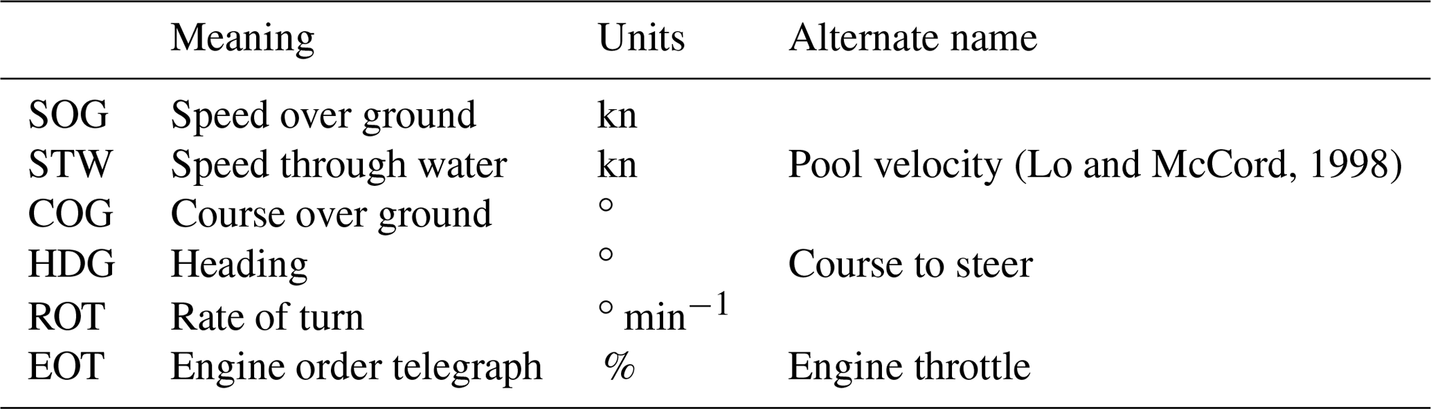
2.1 Basic assumptions
VISIR optimisation corresponds to the top layer in a hierarchical ship motion control system. It determines long-term routing policies that affect the motion of the vessel, viewed as a particle. The related kinematics occur over a long period of time with respect to the timescale of the lower control layer, corresponding to the motion control level, and determine the behaviour of the vessel as a rigid body under the influence of external forces and moments (see Appendix B).
In terms of the nomenclature used, “vehicle” is here used as a more general term than vessel for the theoretical results that do not refer to any specific ship feature. The term “flow velocity” is used for referring to the velocity resulting from either ocean surface current, tidal current, and non-linear mass transport in surface gravity waves (Stoke's shift) or their composition. Also, when not otherwise specified, the qualification “over ground” is assumed for both speeds and courses.
2.1.1 Linear superposition
Assuming that a linear superposition principle holds for vehicle and horizontal flow velocity, the vector speed over ground (SOG) of the vehicle is given by
where F is the vehicle speed through water (STW) and w the flow velocity. The symbol F is a reminder that such speed, due to energy loss in waves, is in general a function of both vehicle propulsion parameters and the ocean state (see Mannarini et al., 2016a, Eq. 21).
Equation (1) is a “no-slippage” condition: the vehicle is advected with the flow. The rationale for this assumption is the experimental observation that ocean drifters (including vessels) adjust their speed to the flow very quickly, i.e. in less than 1 min (Breivik and Allen, 2008). At the present level of approximation, such adjustment is instantaneous (as no second derivatives of x appear in Eq. 1), and it is independent of vessel displacement (no vehicle mass in Eq. 1). In their optimal control methods, Bijlsma (2010) and Techy (2011) make the assumption of linear superposition of speeds. Zamuda and Sosa (2014) do the same as a kinematic basis of an evolutionary approach for describing glider motion. In the context of vessel motion control, Fossen (2012, Eq. 26) defines STW or relative speed as a linear composition of SOG and current velocity.
However, we note that the superposition principle in the form of Eq. (1) only refers to a surface flow and cannot accommodate a depth-dependent (horizontal) flow speed w(z). Thus, vessel speed relative to water should be calculated using the balance between the overall drag by the fluid (Newman, 1977) and the thrust provided by the propulsion system. This can be significant for large draught vessels, especially those sailing in stratified waters (where the vertical profile of water velocity may exhibit both magnitude and direction changes; see Apel, 1987).
Finally, the aerodynamic drag on vessel superstructure is also neglected in Eq. (1).
2.1.2 Course assignment
Along the vessel path, course over ground (COG) may need to be constrained for navigational reasons (traffic constraints, fairways, shallow waters, or any other reason for preferring a specific passage), and in the computation of an optimal path, the algorithm (such as a graph-search method) may resort to spatial and directional discretisation, which again is a form of course assignment.
Making reference to Fig. 1, if COG has to be along , then the vehicle vector velocity must satisfy the following:
where is a normal versor of .
To keep the course constrained as per Eq. (2), it is assumed that the shipmaster can act on the rudder(s) for modifying the heading until COG satisfies Eq. (2) and then report the rudder(s) to the midship.
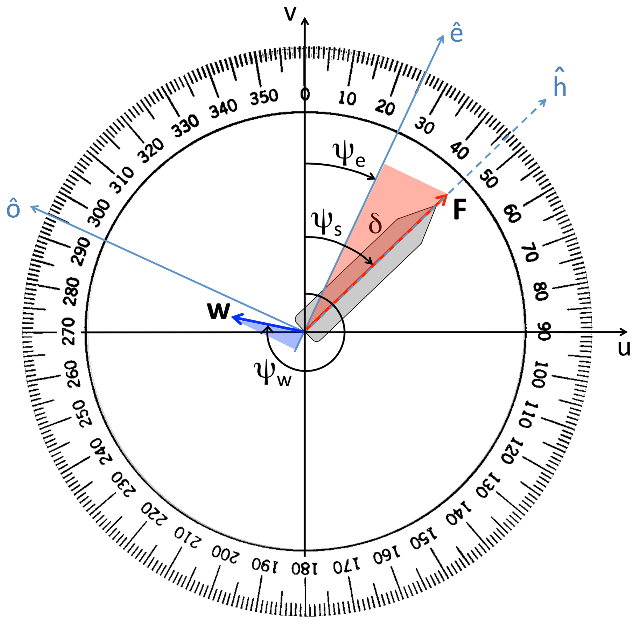
Figure 1VISIR-1.b directional conventions on top of the compass protractor. Shown is the vessel speed through water (F), flow speed (w), vessel COG (ψe), vessel heading (ψs), flow direction (ψw), and angle of attack through water (). The length of the longer cathetus of the blue triangle is equal to the shorter cathetus of the red triangle and represents the cross-current magnitude ; see Eq. (7). The configuration displayed refers to a vessel course assignment () and implies a positive angle of attack (δ=21∘) which balances the drift due to a port-bearing flow w.
2.2 Resulting kinematics
After defining the vector components of the water flow,
and making reference to Fig. 1, the flow projections along () and across the vehicle course (), respectively, are
where for both course ψe and flow direction ψw, the nautical or oceanographic convention (i.e. where-to direction, clockwise from due north) is employed. Furthermore, the choice of orientation of the axis in Fig. 1 implies that a current bears to port whenever .
Linear superposition Eq. (1) and the course assignment condition Eq. (2) result into two scalar equations that, upon definition of an angle of attack δ of the ship's hull through the water (see Richardson, 1997),
as the difference between the angle of vehicle heading (ψs or heading – HDG) and the COG, read
with the unknown Sg being recognised as the vehicle SOG. Remarkably, Eqs. (6a)–(6b) could also be used to determine ocean current vector w given the SOG, STW, course, and heading. As long as F is non-null, δ is given by
In the presence of waves, F is reduced due to the wave-added resistance and can be obtained from a thrust-balance equation as in Mannarini et al. (2016a, Eq. 14). As F is always non-negative, Eq. (7) implies that . In particular, in the case of a crossflow w⊥ bearing to port, a clockwise change of vehicle heading is needed for keeping course, as in the example shown in Fig. 1.
Inserting δ into Eq. (6a), SOG is obtained:
Equation (8) shows that the crossflow w⊥ always (i.e. independently of its orientation) reduces SOG, as part of vehicle momentum must be spent on compensating for the drift. The along-edge flow w∥ (“drag”) may instead either increase or decrease SOG. Notice that the “cross” and “along” specifications refer to vessel course, differing from vessel heading by the (usually small) amount given in Eq. (7). Also it should be noted that a condition,
is not guaranteed in case of a strong countercurrent. In a directed graph (as the one used in VISIR), a violation of Eq. (9) along a specific edge would imply that the edge is made unavailable for sailing along that direction.
An equation formally identical to Eq. (8) was retrieved by Cheung (2017) in the context of flight path prediction, with wind replacing the ocean currents and plane true airspeed replacing vessel STW.
Furthermore, both Eqs. (7) and (8) hold if and only if
If this is not the case, vehicle speed cannot compensate for ocean current drift. We note that Eq. (10) is satisfied even in case of a vehicle drifting along the streamlines of the flow field without any steering (). Equation (1) then reduces to , and vehicle heading is aligned with COG, or
Finally, by taking the module of both sides of Eq. (1) and approximating the l.h.s. (left-hand side) with its finite-difference quotient (thus leading to a first-order truncation error), the graph edge weight δt is computed as
where δx is the edge length. The weights δt are then used for the computation of a time-dependent shortest path, using the same graph-search method described in Mannarini et al. (2016a) and updated in this paper in Sect. 2.4.
2.3 Graph preparation
In this section we report the procedure for ensuring that the graph used by VISIR is safe for navigational purposes. A note on use of non-regular meshes can be found in Appendix C.
Due to the non-convexity of the shoreline and the presence of islands, the maritime space domain is not simply connected, and thus not all graph edges correspond to navigable courses. To account for this, the following graph pruning methodology is used. It starts from the observation that in a large ocean domain, most of the edges do not intersect the coastline. Thus, the procedure consists of the following three steps:
- i.
Retrieve the indices of edges within a small bounding box around each coastline segment.
- ii.
Check edges within the bounding box for intersection with the coastline.
- iii.
Create all edges in the selected domain, pruning just those from the previous step and intersecting the coastline.
The first step can be performed in a constant time with respect to the size of the maritime domain because the graph is based on a structured grid. Furthermore, it can use a lower-resolution version of the shoreline (see Sect. 4.1.2), while the second step must use a higher-resolution.
Thus, when creating the graph, only the sea and land arcs that do not intersect the shoreline are included in the graph. When the code for track computation is then run, for each of the requested track endpoints (i.e. start and end location of the route), the nearest node on the graph is determined. This can even be a land rather then a sea node. In the subsequent step, the graph arcs are screened for the condition that the under keel clearance (UKC) is UKC (Mannarini et al., 2016a, Eq. 44). Thus, if the start node was found on land (UKC ≤0), no outgoing path from that node can be computed and VISIR quits with a warning. The coordinate of the requested endpoint must then be shifted by the VISIR user so that its next node is not on land any more. This requires improvements before it can be used operationally, but for the current assessment exercise, whereby the endpoints are chosen just once and then used for many computations (288 tracks per route; see Sect. 4.5), this approach is still acceptable.
In VISIR-1.a graph nodes were linked only to all other nodes that can be reached via either one or two hops. In this work, a larger number of hops ν is, however, allowed. This enables the angular resolution Δθ to be increased up to
The ν value is also called the “order of connectivity” of the graph (Diestel, 2005). In Mannarini et al. (2019a) the point is made that the numerical solution of the shortest path problem on a graph converges to the numerical truth as ν is increased in roughly inverse proportion to graph mesh spacing Δg1.
The computational cost of VISIR-1.b graph generation procedure is linear in the total number of edges (from step one of the procedure above) within all the bounding boxes around the shoreline. For a given number of nodes, the computation time for preparing a graph of order ν then scales as 𝒪(ν2). More information on the scaling of the method performance can be found in Appendix C.
2.4 Time interpolation of edge weights
As in VISIR-1.a, edge weights are also computed out of Eq. (12) in VISIR-1.b.
The shortest path algorithm is still derived from that of Dijkstra, which is a deterministic and exact method (Bertsekas, 1998). The algorithm was made time-dependent under the assumption that no waiting times at the tail nodes are necessary, or the FIFO hypothesis (Orda and Rom, 1990). Furthermore, a new option is introduced in VISIR-1.b to conduct the time interpolation of the edge weights. Here, the edge weights are not kept constant between consecutive time steps of the input geophysical fields (currents and/or waves) but are estimated at the exact time at which the tail node is expanded by the shortest path algorithm.
In Mannarini et al. (2019a) it was shown that the effect of time interpolation can be relevant wherever the environmental fields rapidly change between successive time steps. This is likely the case for daily averages of the wave fields (Sect. 4.1.4), which are used for the case studies (Sect. 4) of this paper.
Orda and Rom (1990) stated that, under the FIFO hypothesis, the worst-case estimate of the computational performance is, as for the static case, 𝒪(N2), with the N being the number of graph grid points considered2. However, Foschini et al. (2014) pointed out that in the presence of time-dependent edge weights, the computational performance may degrade to become non-polynomial. The scaling of performance with time interpolation (T-interp) is further investigated in Sect. 3.2 through a few empirical tests.
2.5 Vessel modelling
The VISIR-1.b vessel propulsion and seakeeping model is the same as in VISIR-1.a, but with a minor update. It is reviewed and updated in Sect. 2.5.1–2.5.2. Furthermore, under the hypothesis of constant engine order telegraph (EOT), an estimate of the voyage energy efficiency is provided in Sect. 2.5.3.
2.5.1 Vessel speed in a seaway
STW together with the ocean current velocity determines SOG (Eq. 1). SOG in turn determines the edge weights in the graph representation of the kinematical problem (Eq. 12). STW depends on the vessel propulsion system (MANDieselTurbo, 2011) and on the energy dissipated through hydrodynamic viscous forces, aerodynamic forces, ocean surface gravity waves, and waves generated by the vessel through the water displacement (Richardson, 1997). However it is beyond the scope of this paper to develop a vessel propulsion and seakeeping model more realistic than that in VISIR-1.a (Mannarini et al., 2016a).
That model considered the balance of thrust and resistance at the propeller, neglecting the propeller torque equation (Triantafyllou and Hover, 2003). In the resistance, a term related to calm water is distinguished from a wave-added resistance. The calm water term depends on a dimensionless drag coefficient CT, which within VISIR should have a power-law dependence on vessel speed through water: CT=γq(STW)q. For the wave-added resistance, its directional and spectral dependence is neglected, and only the peak value of the radiation part is considered. The latter was obtained by Alexandersson (2009) as a function of the vessel's principal particulars, starting from a statistical reanalysis of simulations based on the method of Gerritsma and Beukelman (1972). By only considering radiation and neglecting the diffraction term, wave-added resistance may be underestimated for long vessels with respect to the wavelength.
2.5.2 Vessel intact stability
In line with IMO guidance (IMO, 2007), VISIR also uses sea-state information to conduct a few checks of a vessel's intact stability. In Mannarini et al. (2016a) ongoing research activity into this topic was noted. Specifically, at that time the development of “second-generation” stability criteria was proposed by Belenky et al. (2011). A recent terms of reference for updating the IMO stability code (IMO, 2008) was published by the (IMO, 2018c).
At present, VISIR includes checks of intact stability related to parametric roll, pure loss of stability, and surf-riding and/or broaching-to at an intermediate level between IMO (2007) and the second-generation criteria. Either intentional speed reduction (EOT <1; Table 1) or course change can be exploited by VISIR for fulfilling the stability checks (Mannarini et al., 2016a).
All vessel speeds at any location and direction (i.e. on each of the A edges) and any time (Nt time steps) are computed ahead of path optimisation (Mannarini et al., 2016a, following Sect. 2.2.2 and pseudocode in Appendix A). A time-dependent Dijkstra algorithm (Mannarini et al., 2016a) can then manage all this spatially and temporally dependent information for computing the time-optimal paths. Its correctness is demonstrated by comparison with the path resulting from the benchmark solution in a dynamic-flow field (Sect. 3.1.2; Fig. 2; Table 2). Similarly, edges that, for a given EOT, violate stability are pruned before the shortest path algorithm is run. Stability loss is assumed to be local in both space and time, no matter what the previous path is before the vessel sails through the edge, violating stability. Thus, the edge is pruned only for that time step ahead of path optimisation.
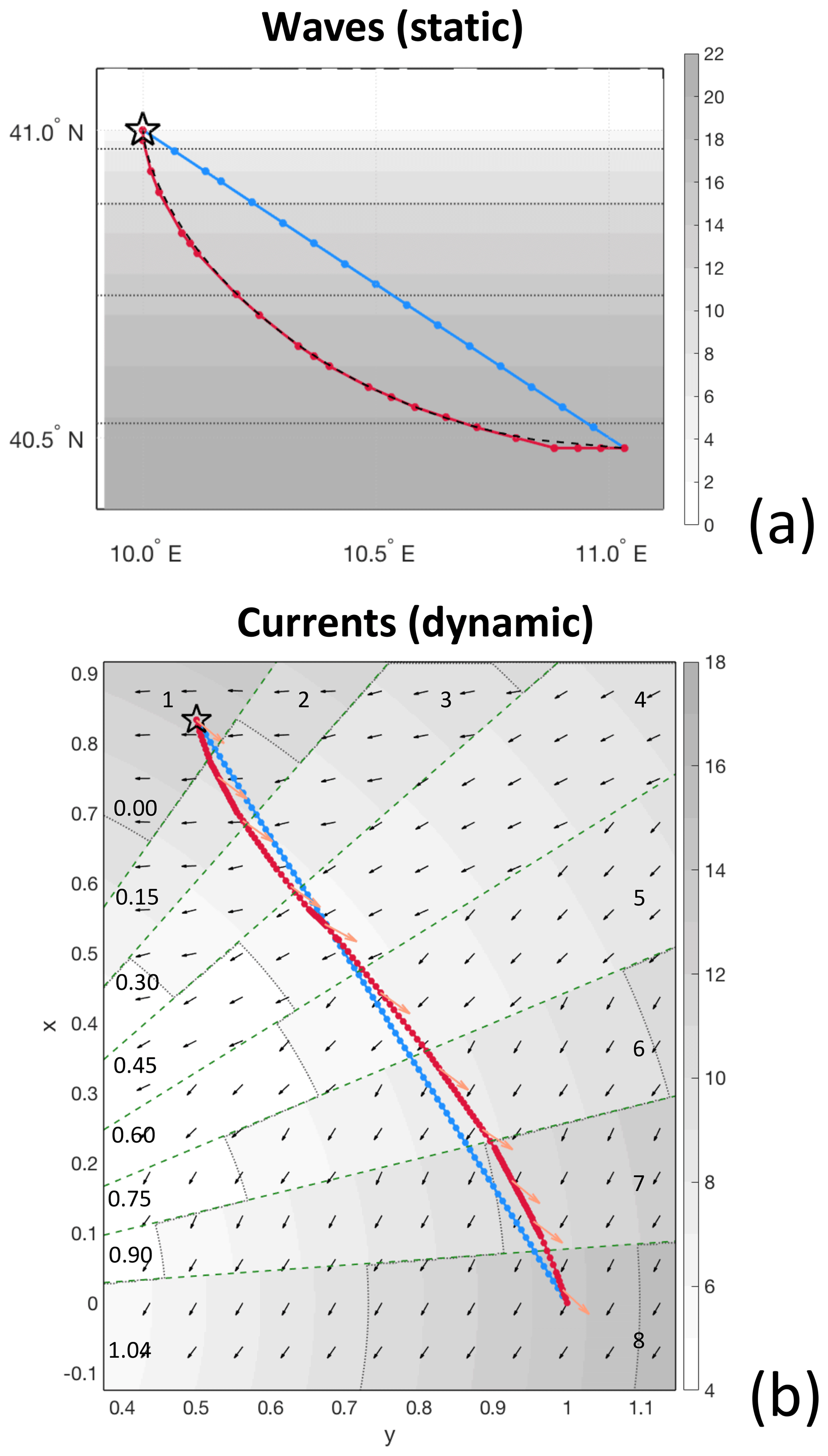
Figure 2Verification of VISIR-1.b vs. benchmark solutions. Both least-distance (blue) and least-time (red) trajectories are displayed, and the tracks originate at the black star symbols. (a) A static ship velocity field as in Eq. (19) is shown; the analytical solution (branch of an inverted descent cycloid) is portrayed as a dashed black line (see Mannarini et al., 2016a, Fig. 9). (b) A time-dependent current field as in Eq. (20); the vehicle heading is portrayed as orange arrows. The radial sectors separated by green dashed lines refer to a sequence of time steps in the field, which are numbered in the outer sector. On the other hand, sector-mean times with a unit of T0 are given in the inner sector. Sectors nos. 3, 6, and 8 should be compared to Techy (2011, Fig. 12a–c). In both (a) and (b), the legend units are knots and velocity field isolines every 5 kn are displayed as dots. Parameters of the synthetic fields are given in Table 2.
Table 2Summary parameters of benchmark case studies (see Fig. 2). Length scale L0 set by the track endpoint distance and timescale are employed throughout (Vmax=21.1 kn). Values in italics correspond to runs without time interpolation of the edge weights (see Sect. 2.4). Values in the last row of each group refer to the analytic solutions.

Therefore in terms of vessel stability, the sole update in VISIR-1.b is in the actual values of the vessel parameters and the parametric roll stability check. The new vessel parameters are suited for modelling a container ship and are listed in Table 4. These values result in an STW dependance on significant wave height as in Fig. 4a and resistance as in Fig. 4b. For the parametric roll, the wave steepness criterion is generalised for vessels of Lwl>100 m by implementing the piecewise linear function of Lwl given by Belenky et al. (2011, Eq. 2.37). Thus the method of Mannarini et al. (2016a, Eq. 32) is replaced by
where the critical ratio Σ is given by
As the stability changes are maximised for a ship length close to the wavelength (Belenky et al., 2011, Sect. 2.3.3), the Σ ratio also represents a critical wave steepness. Thus, Eq. (15) implies that it reduces at larger wavelengths, making the check on loss of stability in rough seas more severe than within the previous (VISIR-1.a) formulation.
2.5.3 Voyage energy efficiency
In this subsection the impact of track optimisation on voyage energy efficiency is estimated.
Following the Paris Agreement (UNFCCC, 2015), anthropogenic climate change is receiving increased attention at both international and regulatory levels. The Intergovernmental Panel on Climate Change recently published a special report on the greenhouse gas (GHG) emission reduction pathway to limit global warming above pre-industrial levels to 1.5∘. It was noted that this would require rapid and far-reaching transitions in energy systems and transport infrastructure (IPCC, 2018).
The third IMO GHG study estimated the share of emissions from international shipping in 2012 to be some 2.2 % of the total anthropogenic CO2 emissions (IMO, 2014). According to the EDGAR database, emissions from international shipping in 2015 were higher than the quota of two countries such as Italy and Spain put together (JRC and PBL, 2016).
In line with the United Nations Sustainable Development Goal 13 (https://sustainabledevelopment.un.org/sdg13, last access: 12 July 2019), an initial GHG reduction strategy was approved by the IMO in April 2018 (IMO, 2018b). It is layered into three levels of ambition, with the second one being “to reduce CO2 emissions per transport work, as an average across international shipping, by at least 40 % by 2030, pursuing efforts towards 70 % by 2050, compared to 2008”. Implementation through short-term, middle-term, and long-term measures is envisaged. The short-term measures include the development of suitable indicators of operational energy efficiency.
The IMO previously introduced the Energy Efficiency Operational Indicator (EEOI) as the ratio of CO2 emissions per unit of transport work (IMO, 2009b). There are several possible definitions of transport work that depend on vessel type. We have restricted our focus to a cargo vessel carrying solely containers, for which transport work is defined as deadweight (DWT) times sailed distance L. In order to estimate the quantity in the numerator of EEOI, the CO2 emissions are taken to be proportional to fuel consumption (IMO, 2009b), ending with
where the CF is a conversion factor from fuel consumption to mass of CO2 emitted, s is the specific fuel consumption, P is the engine brake power, and T is the sailing time. Variations in P are allowed by the VISIR algorithm (Sect. 2.5.2), while s is assumed to be a constant.
If a track is plied at a constant P (i.e. EOT =1), the emissions are then proportional to T, and the EEOI ratio ρβ,α of two tracks between same endpoints and sailed with same DWT is given by
where the subscripts label the β track being compared to the α track. Equation (17) shows that ρβ,α is the inverse ratio of the average speeds along the β and α tracks. The EEOI relative change of β to α track is then given by
If the average speed in the β track is higher than in the α track, then , i.e. a EEOI saving is achieved.
Depending on the subscripts α and β, different types of values will be computed in Sect. 4.4.4 for analysing the benefit of the optimal tracks. A non-constant EOT is accounted for by VISIR. However, for the EOT =1 limiting case, the following general properties can be established:
- i.
If vessel stability checks (Sect. 2.5.1) do not lead to any diversions, the mean speed along the optimal track is never lower than along the least-distance (or geodetic) track. Thus, related EEOI savings are always non negative: .
- ii.
Since currents can be either advantageous or detrimental to SOG (Eq. 8), savings of the optimal tracks of cw type can have any sign with respect to optimal tracks of w type, .
Predicted and recorded EEOIs for a trans-Pacific route are compared in Lu et al. (2015).
VISIR-1.b path kinematics described in Sect. 2 are used for the numerical computation of optimal paths on graphs. In this section, an assessment of VISIR-1.b numerics is provided by means of verification vs. analytical benchmarks (Sect. 3.1) and a test of its computational performance (Sect. 3.2).
3.1 Analytical benchmarks
For the verification, VISIR-1.b includes a verification option to run synthetic fields as the input, instead of those from data-assimilative geophysical models (as described in Sect. 4.1), leading to analytically known least-time trajectories or brachistochrones.
The remainder of the processing (generation of the graph, evaluation of the edge weights, and computation of the shortest path) is identical for both synthetic and modelled environmental fields. However, as identified in Sect. 3.1.1 and 3.1.2 below, the synthetic fields are described in terms of linear coordinates. Thus, the spherical coordinates of the graph nodes are first linearised via an equi-rectangular projection.
3.1.1 Waves
The least-time route in the presence of waves is computed using VISIR by assuming that waves affect the speed through water of the vessel (Sect. 2.5.1). For a static wave field, this leads to an STW that is not explicitly dependent on time. This allows for the least-time path problem to be formulated in terms of a variational problem.
Analytical solutions are available for a subclass of these problems, in which STW depends on only one of the spatial coordinates (Morin, 2007). In particular, if speed through water F depends on the square root of the position, as in
and the initial point is at y=2ℛ, the least-time path is given by (an arc of) a cycloid, with ℛ and g parameters determining length and acceleration, respectively (Broer, 2014; Jameson and Vassberg, 2000). The cycloid presents a cuspid at the initial point, because along a brachistochrone, the region with F=0 has to be quit first. The remainder of the path corresponds to refraction within layers of increasing speed or decreasing wave height, according to Snell's law.
The cycloidal benchmark was also exploited in Mannarini et al. (2016a), where the numerical error of VISIR-1.a in path shape and duration was ascribed to the limited angular resolution (a graph with ν=2 was used).
For VISIR-1.b, we compute graphs of higher connectivity (Sect. 2.3), allowing the cycloidal benchmark to be more closely approached. The results are provided in Fig. 2a and Table 2. A relative error of less than 1 ‰ in T* can be attained by only acting on graph connectivity. This improves the accuracy of VISIR-1.a by about 1 order of magnitude.
The cycloidal solution exploits the fact that a functional of the spatial coordinate is minimised under some necessary conditions provided by the Euler–Lagrange equations (Vratanar and Saje, 1998). The hypotheses leading to these equations are not satisfied in the more general case where the integrand of the functional explicitly depends on time. Instead, an assessment of the VISIR solution in time-dependent waves was conducted by comparison with the numerical results of an exact method based on partial differential equations (Mannarini et al., 2019a). However, the verification of VISIR with time-dependent fields against an analytical benchmark is possible in the absence of waves and the presence of currents, as described in Sect. 3.1.2.
3.1.2 Currents
The optimal control formalism provides the framework for computing extremals of a function, not only explicitly depending on spatial coordinates but also on time (Pontryagin et al., 1962; Bijlsma, 1975; Luenberger, 1979). As the optimal path is controlled by a group of variables, an additional relation (“adjoint equation”) holds. A variant of this approach, the Bolza problem, was used for the computation of optimal transatlantic tracks with a time-dependent STW by Bijlsma (1975). Due to topological constraints, some regions of the ocean are unreachable, and the method involves guessing the initial vessel course, which may hinder the implementation in an automated system. Another variant is the approach of Perakis and Papadakis (1989), which accounts for a delayed departure time and for passage through an intermediate location. However, its outcome is limited to finding only spatially local optimality conditions.
Several benchmark trajectories are provided by Techy (2011) based on Pontryagin's minimum principle (Luenberger, 1979), which uses vehicle heading as a control variable. In particular, in the presence of currents, and for a constant speed F relative to the flow (analogous to STW in the nautical case), an analytical relation between vehicle heading (which is the control variable) and vorticity of any (point-symmetric) current field is demonstrated. The field is given by
where both Γ and Ω may depend on time. For the case study (Techy, 2011, Example 3), the start and endpoints are set at the side of one equilateral triangle, and the third vertex is at the flow origin (). Finally, the duration T* of the least-time path is retrieved through an iteration on the initial heading.
Figure 2b displays the VISIR.b solution to Eq. (20) for a case where Γ is a non-null constant (divergent flow) and Ω (one-half of the vertical vorticity) linearly changes in time as per parameters of Table 2. The resulting optimal path changes its curvature, swinging on both sides of the geodetic track, which is crossed at about one-third of its length (see Techy, 2011, Fig. 12). The elongation of the swinging is quite small, with the optimal path differing from the geodetic by less than 1 % in length. This poses a challenge to the numerical solver on the graph, as many accurate course variations are required over a short distance. Thus, it is not surprising to find that the graph mesh spacing Δg is more critical for achieving convergence than the graph order of connectivity ν. However, this only holds if a time interpolation of edge weights (Sect. 2.4) is used. Otherwise, no significant improvements in T* can be achieved (see Table 2). With VISIR-1.b, a minimum error of about 1.3 % in T* is obtained for the graphs used.
3.2 Computational performance
The computational performance (Sect. 3.2.1) and Random Access Memory (RAM) allocation (Sect. 3.2.2) of the new VISIR model version are assessed here. The major changes in the source code with respect to the version already published (Mannarini et al., 2016a) are summarised in Table A1. All the computations for collecting the data of this section were run on an iMac (processor: 3.5 GHz Intel Core i7; RAM: 32 GB 1600 MHz DDR3). The results are displayed in Fig. 3. Here, the number of degrees of freedom (DOFs) of a VISIR job is given by the product NtA of the number Nt of time steps (i.e. days) and the number A of graph edges. A in turn depends on the number of grid points N comprised within the geographical region selected and on the order ν of the graph. Jobs with DOFs varying over more than 4 decades are considered, corresponding to graph orders .
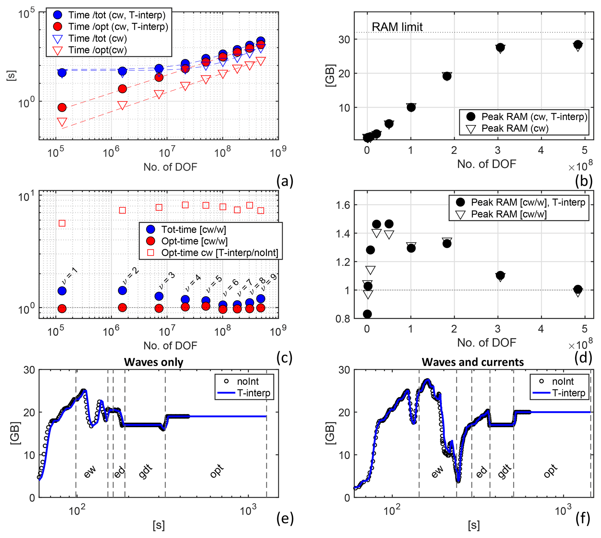
Figure 3(a) CPU time for the total VISIR job (blue markers) and for just the computation of the time-dependent shortest path (red markers). Only the cw case is considered. Dashed lines are fits of the model in Table 3. (b) Peak RAM allocation during the computing jobs of (a), with a reference line at the total installed RAM. (c) Ratio of CPU times between the cw and w cases and (just for optimal path) with and without time interpolation (T-interp). (d) Ratio of peak RAM allocation of the cw- to w-type jobs. For panels (a), (b), and (d), both cases are with (filled markers) and without (empty markers) time interpolation. The DOF of the time-dependent shortest path problems is displayed on the horizontal axis. (e, f) Time series of RAM memory allocation during VISIR execution for w- and cw-type jobs, respectively. Black circles (blue lines) refer to runs without (with) time interpolation of edge weights. Vertical dashed lines separate the main phases of the processing. Both panels refer to the ν=8 case of (a–d). The processing phase labels are as follows: ew (computation of edge-averaged fields), ed (edge delays), gdt (geodetic track), and opt (optimal track).
3.2.1 CPU time
Figure 3a displays both the cost of computing only the optimal track via the shortest path algorithm and the total job cost from its submission to the saving of the results (rendering excluded). Cases without and with time interpolation of the edge weights are distinguished (Sect. 2.4). The CPU time for the optimal track increases almost nearly linearly with the DOF. Below the 107 DOF, a minimum delay of about 1 min can be noticed in the total job cost, which is due to input–output operations. All fitted parameters are reported in Table 3. Asymptotically, it is found that the VISIR time-dependent optimal path algorithm (with time interpolation being active) can be run at a cost of less than 3 µs per DOF. For comparisons to other ship-routing models, see Appendix D.
Table 3Fit parameters for the data displayed in Fig. 3a. The fit model is . For the optimal path data, c parameter is not fitted.

In any two-dimensional regular mesh, the number N of graph grid nodes scales quadratically with the inverse mesh resolution, . For the series of experiments in Fig. 3, we varied ν as 1∕Δg. When taken together, these two effects result in
Thus, the empirically retrieved linearity of CPU time with the DOF corresponds to a quadratic dependence in N. This is in fact the expected worst-case performance of Dijkstra's algorithm (Bertsekas, 1998). In the presence of binary heaps, such an estimate can be reduced to Nlog N. This will be considered in future VISIR versions.
Without time interpolation, the optimal path algorithm is about 8 times faster (Fig. 3c). Furthermore, in Fig. 3c the computational overhead from the use of currents besides waves is assessed. There is no overhead for the shortest path computations (red circles), as they use a set of edge weights of the same size for both cases in the inputs. Instead, edge weight values are determined through the specific environmental fields used (waves alone or also currents). Thus, the preparation of the denominator in Eq. (12) causes an overhead for the total job (blue circles), which is up to 30 % for the sampled DOF range. Starting from ν=8, a rise in the overhead is observed. To understand its origin, the RAM allocation is investigated in the following section.
3.2.2 RAM allocation
Figure 3b shows that peak RAM increases to about 3×10⁸ DOF, where it saturates. Here, the computer's physical memory limit is approached, which leads to swapping and to a degradation of performance, as already observed in Fig. 3c.
This is even more apparent in Fig. 3d, where the ratio of peak RAM for the cw- to w-type computations is displayed. Peak RAM allocation occurs – for large enough jobs – during edge weights preparation, prior to the run of the shortest path algorithm (see ew and opt phases in Fig. 3e and f). There is up to 50 % extra RAM that needs to be allocated if ocean currents are considered. In fact, five environmental scalar fields must be considered (significant wave height, direction, peak period, and zonal and meridional current), but the latter two are not used in the w-type computations. Thus, apart from noise being below 1×10⁸ DOF, a drop of the cw-to-w peak RAM ratio is recorded, as the allocation for the cw case saturates, while, for the w case, it is still significantly lower than such a limit and can grow further. Thus, from Fig. 3d it is possible to define a “computational efficiency region” for VISIR jobs with a DOF lower than the one leading to the drop observed in Fig. 3d. The computations in Sect. 4 are performed on a cluster with a RAM of 64 GB, which can operate in its efficiency region even for larger DOF values.
To further clarify the memory space requirements of VISIR, we focussed on its shortest path algorithm and collected and analysed additional datasets, as described below. These consist of the following:
- d1
-
time series of RAM allocation of the VISIR MATLAB job3,
- d2
-
stopwatch timer readings at specific VISIR processing phases4.
The d2 dataset is then temporally offset by matching the end of the d1 dataset. Finally, the resulting d2 data are smoothed by thinning, which results in the plots displayed in Fig. 3e–f below.
For each graph's angular resolution (indexed by ν parameter), the time series exhibit different relative importance (both in terms of duration and RAM allocation) of the various processing phases. However, the d1 and d2 datasets confirm that, for , the peak RAM is allocated during the edge weight computation (ew phase). Furthermore, the shortest path algorithm is run twice: in its static version (Dijkstra, 1959) for the computation of the geodetic track and in a time-dependent version for the optimal track (Mannarini et al., 2016a). The latter requires the edge delays at Nt time steps in the input, and this justifies the uphill RAM step between these two phases. Finally, Fig. 3e–f proves that time interpolation does not affect RAM allocation but solely CPU time.
In this section, the capacity of VISIR-1.b to deal with both dynamic flows and sea-state fields in realistic settings is demonstrated using the ocean current and wave analysis fields from data-assimilative ocean models.
Section 4.1 presents the environmental fields used for the computations. A documentation of the principal VISIR model settings is presented in Sect. 4.2. A description of the results on individual tracks of a given departure date is given in Sect. 4.3. The analysis of their seasonal variability within a calendar year is conducted in Sect. 4.4, and the extension of such analysis to several routes in the Atlantic Ocean is provided in Sect. 4.5.
4.1 Environmental fields
VISIR-1.b uses both static and dynamic environmental fields obtained from official European and US providers. The static environmental datasets are of the bathymetry and shoreline. The dynamic datasets are of the waves and ocean currents. The specific fields used are described in the following subsections.
4.1.1 Bathymetry
The General Bathymetric Chart of the Oceans (GEBCO) 2014 bathymetric database (https://www.gebco.net/data_and_products/gridded_bathymetry_data/, last access: 12 July 2019; Weatherall et al., 2015) is used in VISIR-1.b. Its spatial resolution is 30 arcsec or 0.5 nmi in the meridional direction.
4.1.2 Shoreline
The Global Self-consistent, Hierarchical, High-resolution Geography Database (GSHHG; https://www.ngdc.noaa.gov/mgg/shorelines/, last access: 12 July 2019) of the NOAA (Wessel and Smith, 1996) is used in VISIR-1.b. There are five versions (c, l, i, h, and f) of the database, with a resolution of about 200 m in the best case. Depending on the geographic domain, VISIR-1.b uses different versions of the GSHHG for the generation of the graph (Sect. 2.3). This limits the generation time in the case of jagged coastlines, such as in archipelagic domains.
4.1.3 Wind
Meteorological fields have not as of yet been used for computing VISIR-1.b tracks. Surface wind fields have only been used in VISIR-1.a for sailboats (Mannarini et al., 2015). Wind also directly affects motor vessels through an added aerodynamic resistance and a heeling moment, which are mainly significant for vessels with a large superstructure, such as passenger ships (Fujiwara et al., 2006). This will be considered in future VISIR developments. We have only used an NOAA Ocean Prediction Center review of marine weather (https://www.vos.noaa.gov/, last access: 12 July 2019) for describing the synoptic situation affecting the ocean state during the periods of the case study of Sect. 4.3. An archive of surface analysis maps (http://www.wetterzentrale.de, last access: 12 July 2019) is also considered.
4.1.4 Waves
Wave analyses are obtained through Copernicus Marine Environment Monitoring Service (CMEMS; http://marine.copernicus.eu/, last access: 12 July 2019) from the operational global ocean analysis and forecast system of Météo-France, based on the third-generation wave model MFWAM (Aouf and Lefevre, 2013).
This uses the optimal interpolation of significant wave height from Jason-2 and Jason-3 and SARAL and CryoSat-2 altimeters. The model also takes into account the effect of currents on waves (Komen et al., 1996; Clementi et al., 2017). Thus, surface currents from the corresponding CMEMS product (see Sect. 4.1.5) are employed and used to force the wave model daily. The currents modulate wave energy and also cause a refraction of the wave propagation. The wave spectrum is discretised into 24 directions and 30 frequencies in the 0.035–0.58 Hz range. Classically, this is the realm of ocean surface gravity waves (Munk, 1951). The vessel intact stability constraints used in VISIR (Sect. 2.5.2) set a timescale given by the vessel natural roll period (usually up to about 20 s or more than 0.05 Hz).
The spatial resolution is 1∕12∘ (i.e. 5 nmi in the meridional direction). Three-hourly instantaneous fields of integrated wave parameters from the total spectrum (spectral significant wave height, mean wave direction, and wave period at the spectral peak) are averaged in a preprocessing stage based on “cdo dayavg” (https://code.mpimet.mpg.de/projects/cdo/, last access: 12 July 2019) into daily fields. Neither Stoke's drift nor the partitions (wind wave, primary swell wave, and secondary swell wave) are used as of yet in VISIR. Due to a much larger fetch, the impact of the swell is estimated to be more significant in the South than in the North Atlantic Ocean (Hinwood et al., 1982).
The wave dataset name is GLOBAL_ANALYSIS_FORECAST_WAV_001_027 (http://cmems-resources.cls.fr/documents/PUM/CMEMS-GLO-PUM-001-027.pdf, last access: 12 July 2019), and the product validation is provided by a companion document (http://cmems-resources.cls.fr/documents/QUID/CMEMS-GLO-QUID-001-027.pdf, last access: 12 July 2019). The datasets were downloaded from CMEMS at least 14 d after their date of validity, ensuring that the best analyses are used.
4.1.5 Currents
Ocean currents are obtained through CMEMS from the operational Mercator global ocean analysis and forecast system based on the NEMO v3.1 ocean model (Madec, 2008).
This uses the SAM2 (SEEK Kernel) scheme for assimilating the sea level anomaly, sea surface temperature, mean dynamic topography (CNES-CLS13), and more. The spatial resolution is 1∕12∘ (i.e. 5 nmi in the meridional direction). Daily analyses of surface fields are used in VISIR-1.b.
The dataset name is GLOBAL_ANALYSIS_FORECAST _PHY_001_024 (http://cmems-resources.cls.fr/documents/PUM/CMEMS-GLO-PUM-001-024.pdf, last access: 12 July 2019), and the product validation is provided by a companion document (http://cmems-resources.cls.fr/documents/QUID/CMEMS-GLO-QUID-001-024.pdf, last access: 12 July 2019). The datasets were downloaded from CMEMS at least 14 d after their date of validity, ensuring that the best analyses were used.
4.2 VISIR settings
For the results shown in this section, optimal tracks are computed on a graph with the order of connectivity of ν=8 (see Sect. 2.3) and mesh spacing . These graph resolution parameters are chosen to strike a compromise between track accuracy (i.e. spatial and angular resolution) and computational cost of the numerical jobs (see the discussion in Sect. 3.2). The computations refer to a container ship, and the parameters are reported in Table 4. The resulting vessel's performance in waves is summarised in Fig. 4.
Table 4Database of vessel propulsion parameters and principal particulars used in this work. The values of Δ (ballast minus scantling range) and the maximum cargo capacity (2500 TEUs – 20 ft equivalent units) are not used in the computations and are provided just for the sake of reference.
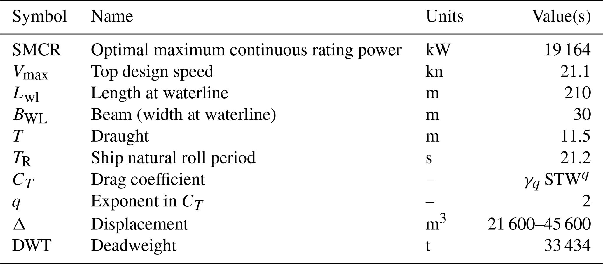

Figure 4Vessel response functions for the parameters given in Table 4. (a) STW at a constant engine throttle vs. significant wave height Hs. Both EOT =100 % (solid line) and EOT =10 % (line and dots) are displayed. (b) Calm water Rc, wave-added resistance Raw, and their sum Rtot as functions of Hs.
4.3 Individual tracks
We first consider a transatlantic crossing in the North Atlantic Ocean, located between Norfolk (USNFK), at the mouth of the Chesapeake Bay ( N, W), and Algeciras (ESALG), just past the Strait of Gibraltar ( N, W). Both east- and westbound tracks are considered (Fig. 5).
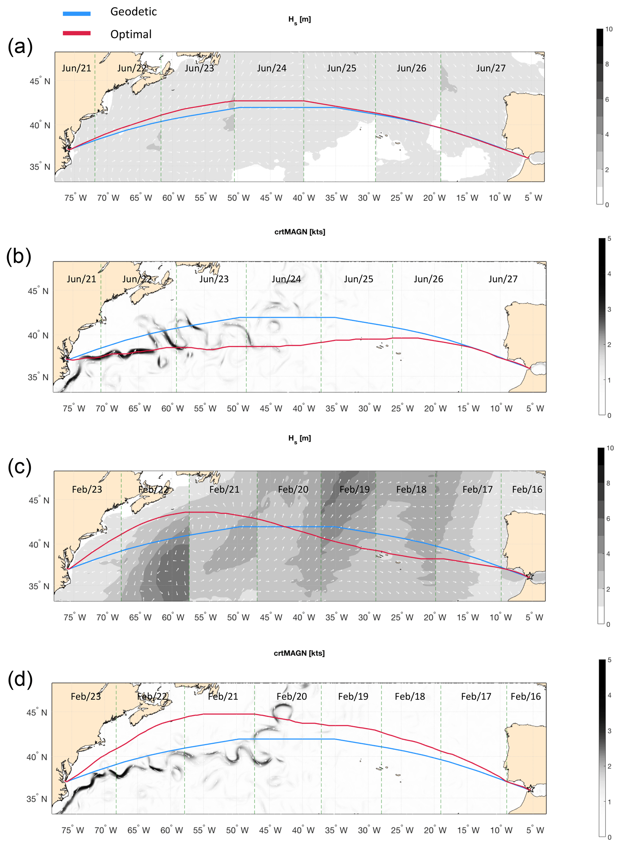
Figure 5Geodetic (blue) and optimal tracks (red) for the USNFK–ESALG route in the presence of different environmental forcings and departure dates: panels (a) and (c) are of w type, Hs is displayed as shading, and wave direction is displayed as white arrows. Panels (b) and (d) are of cw type, current magnitude is displayed as shading, and its direction is displayed as white arrows. Departure date is 21 June for (a) and (b) and 16 February for (c) and (d). Departure time is 12Z (12:00 UTC) for all tracks. All panels are split into vertical stripes relative to daily time steps of the optimal tracks – the interface between stripes is marked by a green dashed line. Summary data are reported in Table 5.
First of all, we note that the geodetic (or least-distance) track is bent northwards, as it is to be expected from an arc of GC of the Northern Hemisphere on an equi-rectangular projection. The track is piecewise linear, and its northern edge is flattened due to the finite angular resolution of the graph: from Eq. (13). However, as Table 5 reports, the error in the length of the geodetic route made by VISIR is only a few per mil. This is comparable to the accuracy of the function for the computation of distances on the sphere (used in VISIR) compared to the ellipsoidal datum (which is more accurate but slower).
For these tracks, meteo-marine conditions are first introduced (Sect. 4.3.1), and track spatial and dynamical features are then discussed in Sect. 4.3.2 along with the impact on vessel stability in Sect. 4.3.3 and their base metrics in Sect. 4.3.4.
4.3.1 Meteo-marine conditions
The synoptic situation in the North Atlantic during the week following 21 June 2017 (departure date for the eastbound track) was dominated by the Azores High blocking descent of subpolar lows to the middle latitudes. This led to relatively calm ocean conditions (significant wave height Hs<5 m) for most of the region involved in the Norfolk–Algeciras crossing.
In the week following 16 February 2017 (departure date for the westbound track) a low with storm-force winds that formed near (41∘ N, 52∘ W) was observed, which then moved N, influencing wave direction on the 19 and 20 February. On 22 February another storm with waves of Hs>8 m developed (37∘ N, 58∘ W).
In terms of the currents, we note that the eastern edge of the crossing is N of Cape Hatteras and, thus, N of the GS branch known as the Florida Current (Tomczak and Godfrey, 1994).
4.3.2 Track spatial and dynamical features
The topological and kinematical features of the optimal tracks of the case study are discussed in this subsection.
Track topology
Four different solutions for the optimal tracks of the USNFK–ESALG route are given in Fig. 5 (red lines).
For the eastbound voyage, when only considering waves (w type; Fig. 5a) the optimal track is quite close to the geodetic track. This is due to the absence of waves of relevant height along the path during the crossing (about 8 d; see Table 5). Discontinuities are seen between significant wave height fields at consecutive time steps (vertical stripes separated by dashed lines). This is enhanced by the daily averaging of the original 3-hourly fields (see Sect. 4.1.4).
When the optimal track is computed for the same departure date and direction but also considers ocean currents too (cw type), the solution is significantly modified (Fig. 5b). A diversion S of the geodetic track is computed by VISIR-1.b. This is instrumental in exploiting advection by the GS through velocity composition (Eq. 8). Despite being longer in terms of sailed miles, this track is faster than the geodetic track (Table 5). A closer look at Fig. 5b reveals that the optimal track averages between the locations of opposite meanders of the first six oscillations of the GS proper, at 72–63∘ W. Subsequent meanders, which are prone to extrude filaments (and are thus more stretched in the meridional direction), are followed increasingly loosely by the optimal track.
On the westbound voyage of w type (Fig. 5c) the optimal track takes diversions both S and N of the geodetic track. This longer path can be sailed at an higher SOG than the geodetic track, because it skips both the storm in the northeastern Atlantic at Δt=1–4 d since departure and the storm developing at Δt=6 d at the latitude of the arrival harbour.
The optimal track for the same departure date and direction but different cw type (Fig. 5d) leads to yet another solution with respect to the w-type track. It sails N of the geodetic at all times. The speed loss due to the encounter with the storm at Δt=2–3 d is balanced by the speed gains due to a meander of the North Atlantic current encountered at Δt≈4 d at 44∘ N and by the benefit of sailing slightly further away from the rough sea than the corresponding w-type track at Δt=5–6 d.
Tracks kinematics
To gain a deeper insight into the results, in Fig. 6, a few kinematical variables are extracted along both the optimal and geodetic tracks for both cw and w cases.
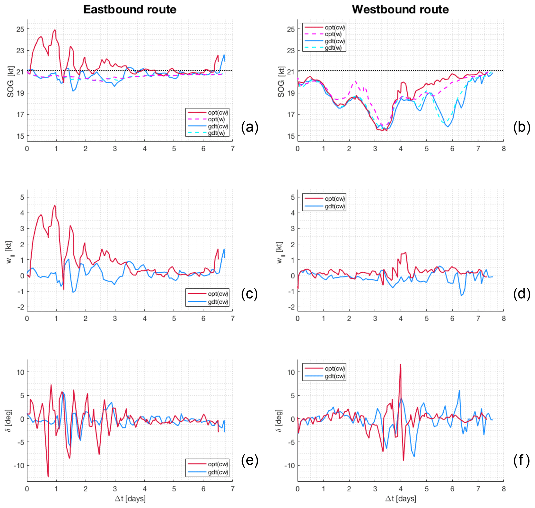
Figure 6Along-route information for both the eastbound (a, c, e) and westbound (b, d, f) crossings of Fig. 5. The first row (a, b) displays the SOG for both optimal and geodetic tracks for both w and cw cases; the black dotted line is Vmax from Table 4. The second row (c, d) displays the w∥ component of the ocean flow, as computed from Eq. (4a). The third row (e, f) displays the angle of attack δ from Eq. (5). The maximum ROT of δ is 0.8 and 0.5 for the east- and westbound track, respectively.
Starting from the eastbound route (Fig. 6a), the SOG of the cw optimal track differs greatly from the corresponding geodetic track. SOG gains by up to more than 4 kn are experienced in the first half of the path due to the GS. During the final part of the navigation (Δt≈6.5 d), an SOG >22 kn peak appears to be shifted in both tracks. This is the signature of the Atlantic jet past Gibraltar, which is encountered about 5 h earlier along the optimal track (see bottom of Fig. 6c). Instead, the SOG does not appreciably differ when w-type optimal and geodetic tracks are compared. This is consistent with the spatial pattern seen in Fig. 5a.
The geodetic westbound track displays heavy oscillations in SOG, with two deep local minima at Δt≈3 and 6 d (Fig. 6b). These correspond to the two storms NE and SW of the track mentioned earlier. The SOG differs from that along the geodetic track just at Δt≈1.5–3 d, along the optimal track of w type, and this is due to its initial northbound diversion. Starting from Δt=4 d both optimal tracks significantly differ from the geodetic track, with the cw track being confirmed as enabling the larger SOG in the second part of the crossing.
In Fig. 6c–d the ocean flow component w∥ along vessel course (Eq. 4a) is displayed. This quantity, together with its normal counterpart w⊥, determines, through Eq. (8), the value of SOG. The difference between the optimal and the geodetic tracks is noticeable for both east- and westbound navigation. In Fig. 6c it can be seen that the algorithm manages to encounter a w∥ that is nearly always positive (i.e. along the course), which even exceeds 4 kn at the end of the first day. It is apparent that the same w∥ oscillations are retrieved in the SOG line chart of Fig. 6a for Δt<3 d and at the Δt≈6.5 d peak. For westbound navigation, w∥ is mainly positive (apart from the initial impact of the Atlantic jet before Gibraltar is passed) along the optimal track and is mainly negative along the geodetic track, which sails against the GS. At Δt=4 d a NW-bound meander of the North Atlantic current is encountered, with a positive drag of up to 1.5 kn.
Finally, the angle of attack δ needed for balancing the crossflow w⊥ (Eq. 5) is displayed in Fig. 6e–f. The track average of δ is nearly zero, its maximum value is of the order of 10∘, and its amplitude is larger wherever is larger. The oscillations of δ with a larger elongation are a signature of the crossing of strong meanders, as seen in the first half of Fig. 6e and at Δt=4 d in Fig. 6f.
Per Eq. (5), δ comprises both the vessel heading and course fluctuations. As shown in Fig. 5, the latter are not too strong compared to those of the geodetic track. Thus, the question is if the heading fluctuations corresponding to the δ signals in Fig. 6e–f are compliant with vessel manoeuvrability. The maximum module of the rate of turn (ROT) of HDG is found to be 2.9 for the eastbound track and 1.5 for the westbound track of cw type. These values are comparable to the IMO prescribed accuracy of 1.0 for on-board ROT Indicators (IMO, 1983). Thus, heading fluctuations computed by VISIR-1.b for this route should be feasible with respect to manoeuvrability.
4.3.3 Safety of navigation
The stability constraints given in Sect. 2.5.2 were checked. However, some of them did not result in any graph edge pruning during the actual transatlantic crossing of the vessel under consideration (see parameters in Table 4). In fact, pure loss of stability was not realised, as the threshold condition of the significant wave height of Mannarini et al. (2016a, Eq. 36) was not reached. Surf-riding and/or broaching-to was not activated due to the condition that the Froude number was never larger than the critical number for the wave steepness encountered (Mannarini et al., 2016a, Eqs. 42–43). By using the generalisation discussed in Sect. 2.5.2, parametric roll could instead occur for the present vessel parameters and the North Atlantic wave climate.
In addition, on this specific route and these departure dates, the voluntary speed reduction (Sect. 2.5.2) was not found to be activated by the algorithm. This means that the tracks are sailed at a constant P and that the CO2 emissions are linearly proportional to the sailing time T* (Sect. 2.5.3). Instead, for other routes in the Atlantic, this is not always the case (see Table 7).
Furthermore, all time-dependent edge weights along the optimal tracks fulfil the FIFO hypothesis (Sect. 2.4).
4.3.4 Track metrics
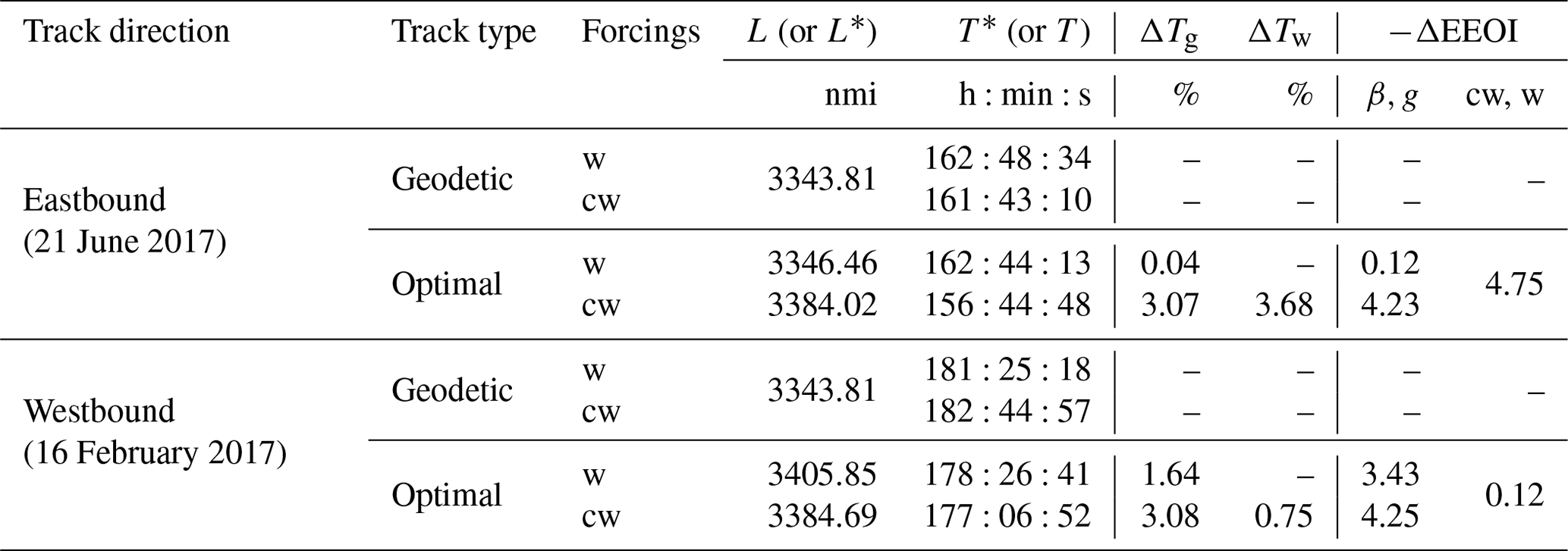
Two simple metrics for summarising the kinematics of a track are proposed here: the optimal track duration T* and the corresponding length L (not a starred symbol, as this length is not the object of the optimisation). For the geodetic tracks, optimisation is instead performed on length L*, and, unless safety constraints play a role in the actual optimal track, the corresponding duration T is higher than T*.
L is sensitive to the geometrical level of the track diversions, while T* reflects their kinematical impact. Such key metrics are reported in detail for both the geodetic and optimal tracks of both the east- and westbound crossings in Table 5. The data also allow us to distinguish the quantitative role of waves and currents and the level of the track duration gains. For example, it is seen that both east- and westbound tracks lead to time savings ∼3 % with respect to the geodetic track. However, for the former, such a saving is mainly due to the exploitation of currents, while the latter is due to waves.
Concerning time gains, it is important to specify whether they refer to the geodetic track (ΔTg) or to an optimal track computed in the presence of waves only (ΔTw). Here, we observe that both Lo and McCord (1995) and Chang et al. (2013), not using waves, only consider ΔTg. In addition, the model region chosen for their track optimisation almost coincides with the domain where the western boundary current under consideration is at its strongest. This is different from the case study presented in this section, which also entails the eastern part of the ocean, where the influence of the western boundary current is less noticeable. Thus, the ΔTg gains due to currents reported in Table 5 are lower than the results in the literature, although they are possibly more realistic when referring to full transatlantic crossings.
4.4 Track seasonal variability
In this subsection we consider the extent to which the seasonal variability in the ocean state and circulation affects the variability in the optimal track of a given transatlantic crossing.
In order to address it, VISIR-1.b computations are conducted for departure dates spanning the whole calendar year 2017. Departures on six dates (1st, 6th, 11th, 16th, 21st, and 26th) in each month are considered, resulting in 72 dates per year. This is aimed at considering the decorrelation of the ocean current fields after a Lagrangian eddy timescale of about 5 d (Lumpkin et al., 2002). As waves are mainly driven by winds, whose velocity is 1 order of magnitude larger than ocean velocities, the timescale for the decorrelation of the ocean state is expected to be even shorter.
To analyse the massive data resulting from these computations, four levels of analysis are considered: spatial variability in the tracks (Sect. 4.4.1), their kinematic variability (Sect. 4.4.2), the distribution of duration T* and length L, (Sect. 4.4.3), and the impact on voyage energy efficiency (EEOI; Sect. 4.4.4).
4.4.1 Spatial variability
A direct visualisation of the annual variability in the track topology is shown in Fig. 7.
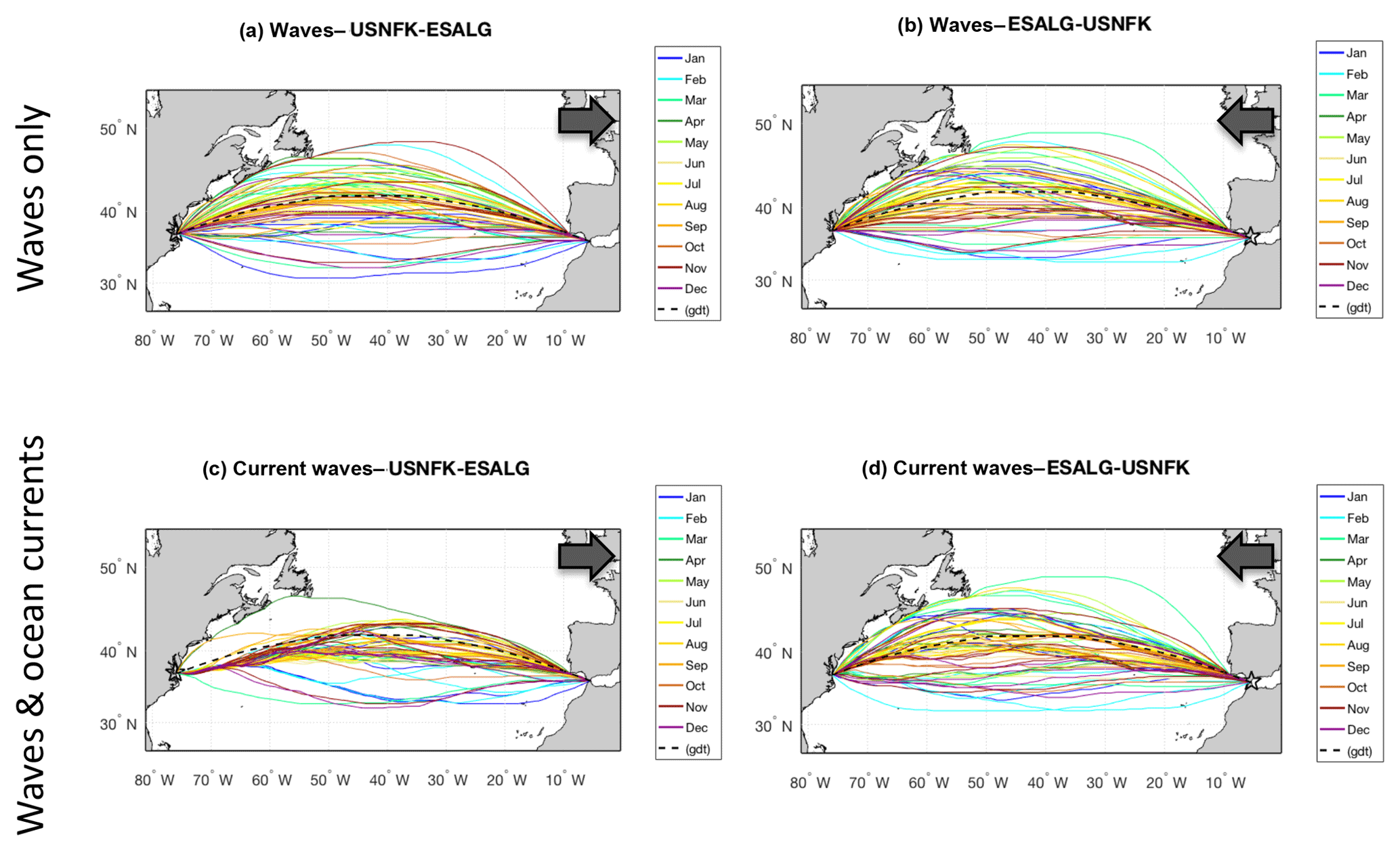
Figure 7Route tracks of the same transatlantic crossing of Fig. 5 during the calendar year 2017. Panels (a) and (b) refer to w type; (c) and (d) refer to cw-type tracks. Both east- (left) and westbound tracks (right) are shown. The geodetic route is displayed as a black dashed line. Animations of the panels are available at https://av.tib.eu/series/560/gmdd+18 (last access: 12 July 2019). For this and other routes, see also the Supplement.
Each panel displays a bundle of trajectories relative to the 72 departure dates. The extent of the diversions makes it clear that the case study of Sect. 4.3 is not even extreme. Instead, for both east- and westbound tracks, the summer and autumn tracks are closest to the GC track because in the North Atlantic Ocean, wave heights tend to be smaller in these seasons, and consequently, both vessel speed losses and relative kinematic benefits from diversions are smaller.
Some tracks are found to sail quite far inshore towards the Canadian coast, and for this we refer to a related comment in Sect. 4.5.4.
The general impact of ocean currents on eastbound tracks is that the bundle of tracks squeezes and shifts S in the vicinity of the GS proper (W of 67∘ W). On a few dates (mainly in winter and spring) this is not the case, as storm systems happen to cross the location of the GS. For the westbound tracks, also accounting for currents only adds a small perturbation to the wave-only tracks without dramatically changing their topology.
It should be stressed that the computed spatial variability depends heavily on how ship energy loss in waves is parametrised (see Sect. 2.5.1). Wave-added resistance determines vessel STW for any given sea state and thus how profitable a diversion to avoid speed loss is.
4.4.2 Evolution lines
While the paths of the tracks displayed in Fig. 7 convey the information about the spatial variability and its seasonal dependence, they fail to provide information about vessel kinematics along the tracks. Thus, an alternative visualisation is proposed in Fig. 8. Following a practice used in track anomaly detection (Zor and Kittler, 2017), cumulative sailed distance is displayed vs. time elapsed since departure. Thus, the slower parts of each path result in a smaller slope for corresponding segments of the track “evolution line”. It can be seen that such slow segments are more frequent in winter months and in the middle of the crossing, particularly for westbound tracks, due to larger speed losses in waves.
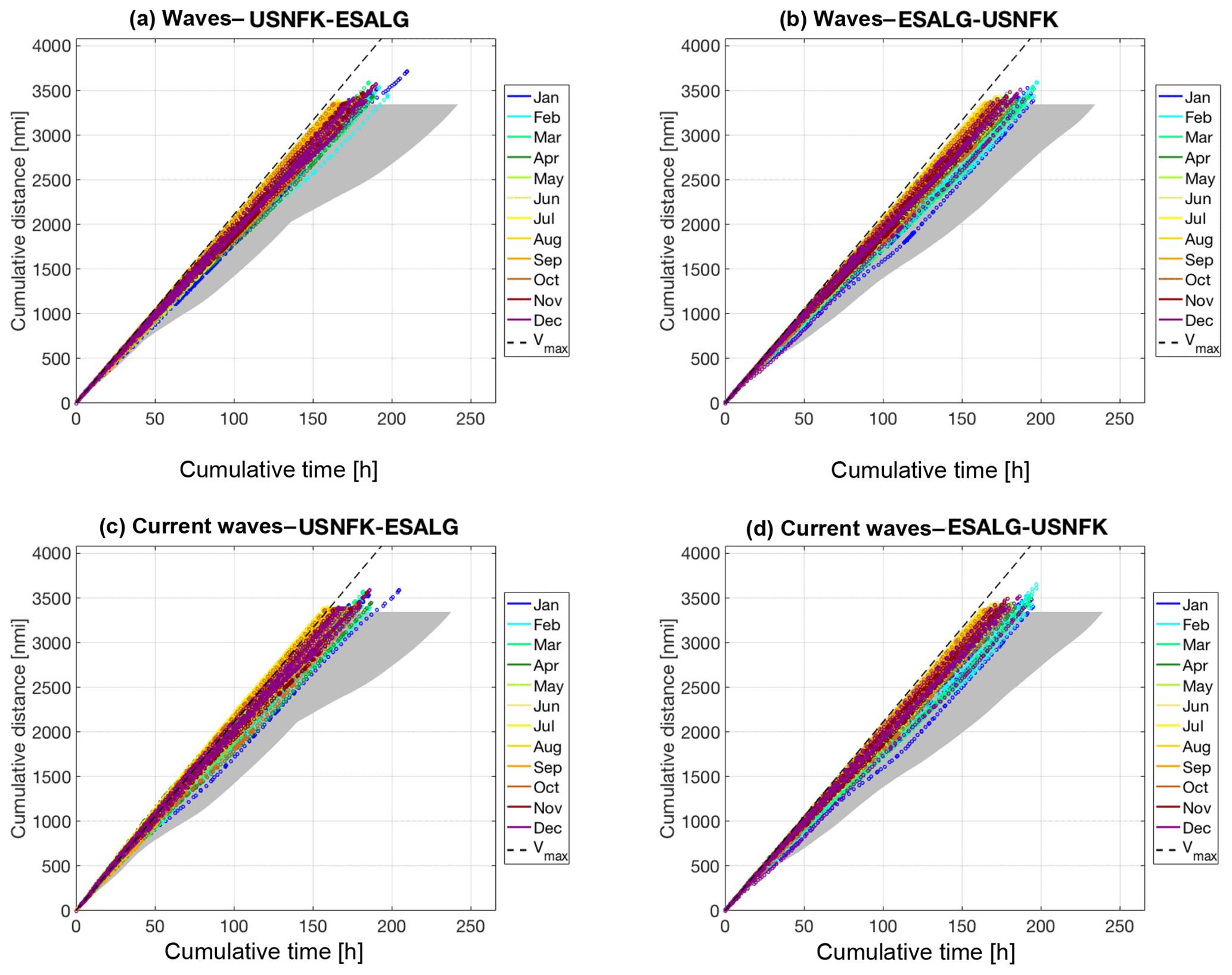
Figure 8Evolution lines for the tracks in Fig. 7: cumulative sailed distance is displayed vs. time elapsed since departure. Each optimal track is displayed with a coloured dot referring to the month of departure as in the legend. The envelope of the geodetic trajectories is shaded in grey. The dashed line refers to sailing at Vmax.
Furthermore, in the presence of currents, the slope can exceed that relative to navigation at SOG equal to the maximum STW. This is due to the speed superposition per Eq. (8) and is apparent for some of the summer tracks in the panel relating to the eastbound tracks (Fig. 8c).
Finally, the envelope of the evolution lines along the geodetic tracks is displayed as a grey shaded area. This reveals the kinematical benefit of the optimal tracks, as they can be sailed at an higher SOG (coloured dots are generally left of the grey areas), resulting in shorter voyage durations.
4.4.3 Scatter plots
To reduce and better analyse the information contained in Fig. 8, the compound metrics T* and L can be used, which are reported in a Cartesian plane in Fig. 9.
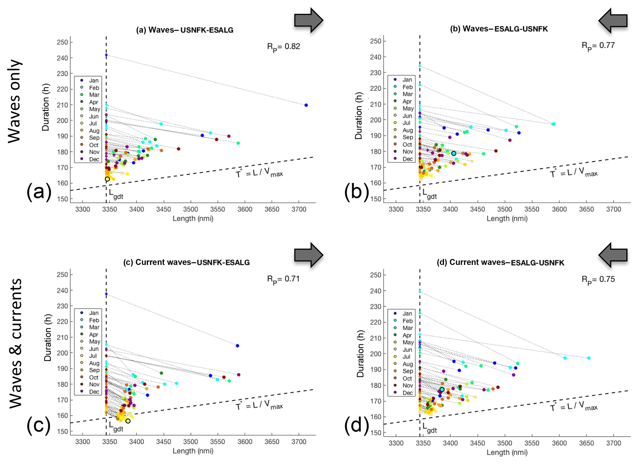
Figure 9Distribution of optimal sailing time T* vs. length L of the tracks of Fig. 7. For the geodetic tracks, L=Lgdt is a constant. Corresponding optimal track dots () are joined by a light dotted line. The slanted dashed line has a slope . Tracks for w-type (a, b) and cw-type optimisation (c, d), and for both east- and westbound directions, are displayed. Dots of the tracks analysed in Sect. 4.3 are outlined in black. Pearson's correlation coefficient RP between T* and L is printed in the top right corner of each panel.
Such a plane contains a strictly forbidden region, left of L=LGC, which is the length (on the graph) of the GC arc connecting the route endpoints. The straight line through the origin, whose slope is , generates another relevant partitioning of the plane. In fact, the region above this line corresponds to tracks sailed at an average speed lower than Vmax, and the region below this line corresponds to tracks sailed at an average speed higher than Vmax.
We first focus on eastbound tracks. The distribution for w-type tracks is given in Fig. 9a. As expected, they are all comprised within the region above the line. This is due to involuntary speed loss in a seaway, which reduces the average speed to less than Vmax. When currents are also considered (Fig. 9c), the tracks can be faster, and for eastbound navigation, some of them even attain the region where the average SOG is larger than Vmax. This generally occurs for summer tracks, which experience a lower speed loss in waves.
For the westbound tracks (Fig. 9b–d), the general picture differs in terms of the following features: the region where the average vessel SOG is larger than Vmax is never attained, and the distribution in the () plane roughly maintains its pattern among the w- and cw-type results.
These findings are also mirrored in Pearson's correlation coefficient RP between T* and L. While for the westbound tracks RP is nearly unchanged (Fig. 9b–d), it decreases substantially between Fig. 9a and c. Most eastbound tracks, independently of their duration, require a significant diversion to exploit the GS proper. This in turn reduces the correlation between T* and L.
The dots relative to the tracks selected for the featured analysis of Sect. 4.3 are seen as circles in Fig. 9. For the eastbound crossing, a transition into the efficiency region is seen when comparing the w-to the cw-tracks.
Table 5Route length L (or L* for geodetic tracks) and optimal duration T* (or T for geodetic tracks) for tracks in Figs. 5–6. ΔTg is the relative duration change with respect to the geodetics; ΔTw is the relative duration change with respect to w-type optimal tracks. On the WGS-84 geoid, the length of the arc of GC between the endpoints is 3332.60 nmi; i.e. the numerical solution overestimates it by 0.3 %. In a still ocean (no currents or waves), the numerical geodetic would be sailed in h by a vessel with Vmax as in Table 4. The second header line of the −ΔEEOI columns specifies the type of tracks as in Eq. (18).
4.4.4 EEOI savings
For assessing the benefit of track optimisation in terms of voyage energy efficiency, in Fig. 10, the monthly and annual variability in the EEOI savings is displayed.

Figure 10EEOI relative savings for the tracks in Fig. 7. The quantity defined in Eq. (18) is computed for optimal tracks of cw type vs. (a, b) the corresponding geodetic tracks and (c, d) vs. corresponding optimal tracks of w type. For each calendar month, the empty circle is positioned at the monthly average, and the error bars span between minimum and maximum value of the (six) routes of that month. w/r introduces the type of optimal track with respect to which the EEOI savings are computed.
In reference to Sect. 2.5.3, specific fuel consumption s is taken to be a constant, while engine brake power P is allowed to vary as EOT is selected by the optimal routing algorithm (see Sect. 2.5.2).
With the notation of Eq. (18), EEOI savings of the tracks considering both ocean currents and waves (β= cw) are computed with respect to either the geodetic track (α=g; Fig. 10a–b) or the wave-optimal tracks (α=w; Fig. 10c–d).
For the eastbound route, −Δ(EEOI)cw,g exhibits a clear seasonal cycle, with a peak of the monthly mean value in winter. However, the winter intra-monthly variability exceeds the amplitude of the seasonal cycle. For the westbound route, these trends are still observed, but both the seasonal cycle and the intra-monthly variability are less regular.
Furthermore, in Fig. 10c–d the monthly mean value of −Δ(EEOI)cw,w is found to be larger for the eastbound route, as it can benefit from advection by the GS. Peak values of −Δ(EEOI)cw,w are found in summer months, when the ocean state is calmer, and thus the relative contribution of currents is the prevalent one.
Thus, the magnitude and location of the GS is critical for voyage energy efficiency along this route in summer. In this respect, Minobe et al. (2010) found, from satellite altimetry data, that the seasonal cycle of the geostrophic component of the GS is weak both in terms of meridional position and near-surface velocity. The simulations of Kang et al. (2016) instead show a seasonal cycle of the mean kinetic energy of the GS proper, with a relative maximum during summer. Berline et al. (2006) analysed the GS latitudinal position at 75–50∘ W from model reanalyses and found that inter-annual and seasonal variability dominates upstream and downstream of 65∘ W, respectively.
4.5 Ocean-wide statistics
The degree of optimisation of ship tracks that were actually sailed is an open research question. Weather ship-routing systems are used both offshore and on-board for planning, but the final decision is up to the shipmaster (Fujii et al., 2017). Furthermore, route planning may involve sensitive commercial information that a ship operator will not easily share. Thus, the extent to which a ship track is optimised is not always publicly known. We recently addressed this question by comparing VISIR optimal tracks based on wave analysis fields vs. reported ship tracks per AIS (Automated Identification System) data for a route in the Southern Ocean (Mannarini et al., 2019b). By computing both spatial and temporal discrepancies between VISIR and AIS tracks, we could infer that optimisation likely took place in several but not all tracks.
VISIR can be used with either analysis or forecast environmental fields, as it is not constrained by any of the equations of Sect. 2. Thus, VISIR can help both predict optimal tracks (as actually done in the operational system for the Mediterranean Sea described in Mannarini et al., 2016b) or assess past tracks (as we do in the present work). Transatlantic crossings may in some cases be longer than 10 d and thus exceed the maximum lead time of wave forecast model outputs, which are limited by the availability of related atmospheric forcing fields. The lead time of CMEMS products is limited to 10 d for ocean current forecasts and to just 5 d for wave forecasts (see product user manuals cited in Sect. 4.1). To our knowledge, although European Centre for Medium-Range Weather Forecasts (ECMWF; https://www.ecmwf.int/en/forecasts/datasets/set-ii, last access: 12 July 2019) runs a global wave model based on WAM with a 10 d lead time, it has a lower spatial resolution (1∕8∘) and no-open-access policy, while NCEP (https://polar.ncep.noaa.gov/waves/hindcasts/prod-multi_1.php, last access: 12 July 2019) runs a model based on WW3 on various grids and with a lead time of 7.5 d (https://www.ncdc.noaa.gov/data-access/model-data/model-datasets/global-forcast-system-gfs, last access: 12 July 2019).
The unavailability of forecasts that are long enough can be addressed by either rerouting or using supplementary information. Rerouting or replanning involves the dynamic updating of the optimal track as new information (forecast) is made available (Stentz, 1995; Likhachev et al., 2005). The corresponding solution is suboptimal, as the initial routing choices are unrecoverable and may compromise the attainment of a globally optimal solution. An example of the use of supplementary information instead has been proposed by Aendekerk (2018). Here, a “blending” of climatologies and geometrical information is used as a surrogate for missing forecasts with long lead times.
In a non-operational mode, the unavailability of forecasts is not critical. Analysis fields can then be used, enabling a better reconstruction of the environmental state. A product derived from analyses may be quite useful for scenario assessment, but the uncertainty associated with forecasts (Bos, 2018) complicates its usefulness. Analysis fields of waves and ocean currents are used throughout the present paper.
For nine ordered couples of harbours from the list in Table 6, 72 tracks relative to year 2017 are computed. Two sailing directions and both w and cw cases are considered, leading to the computation of 288 tracks per route per year. This results in the computation of more than 2500 tracks in the Atlantic Ocean with the same VISIR-1.b code version.
Table 6Database of harbours. Coordinates refer to the graph grid point selected by VISIR. Wherever available, GRT is the annual throughput for the year 2016 from Lloyd's (2018) and is used for sorting the entries. The other harbours are sorted alphabetically, following international seaport codes.

This exercise demonstrated the generality of the VISIR-1.b code for assessing the potential EEOI savings depending on various wave and ocean circulation patterns. This required that graph, shoreline, bathymetry, and environmental datasets of waves and ocean currents, among other datasets, be made available for wide enough regions of the Atlantic Ocean to account for the spatial variability in the tracks.
By using Table 7 and Fig. 11, the obtained general results can be summarised as follows:
- a.
EEOI savings in the North Atlantic are dominated by waves, with a contribution from currents that is not negligible. At the Equator, currents are the main reason for EEOI saving. In the South Atlantic, the largest savings are computed, and they are mainly due to waves.
- b.
Routes mainly affected by ocean currents exhibit a large reduction of the correlation coefficient RP when comparing w- to cw-type scatter plots of track duration vs. track length.
- c.
The FIFO hypothesis is not satisfied in just a tiny number of edges, which are not used for the optimal tracks. This supports the use of the time-dependent Dijkstra algorithm, as in Sect. 2.4.
- d.
Intentional vessel speed reduction (EOT <1) occurs in just three routes and for a relatively limited proportion of their track waypoints. This supports the approximation conducted in Sect. 2.5.3 for estimating the relative EEOI savings.
- e.
Maximum ROT never exceeds 20. Given that COG changes are smooth (see e.g. Fig. 5), ROT changes reflect the HDG adjustments for balancing either strong or variable cross-currents.
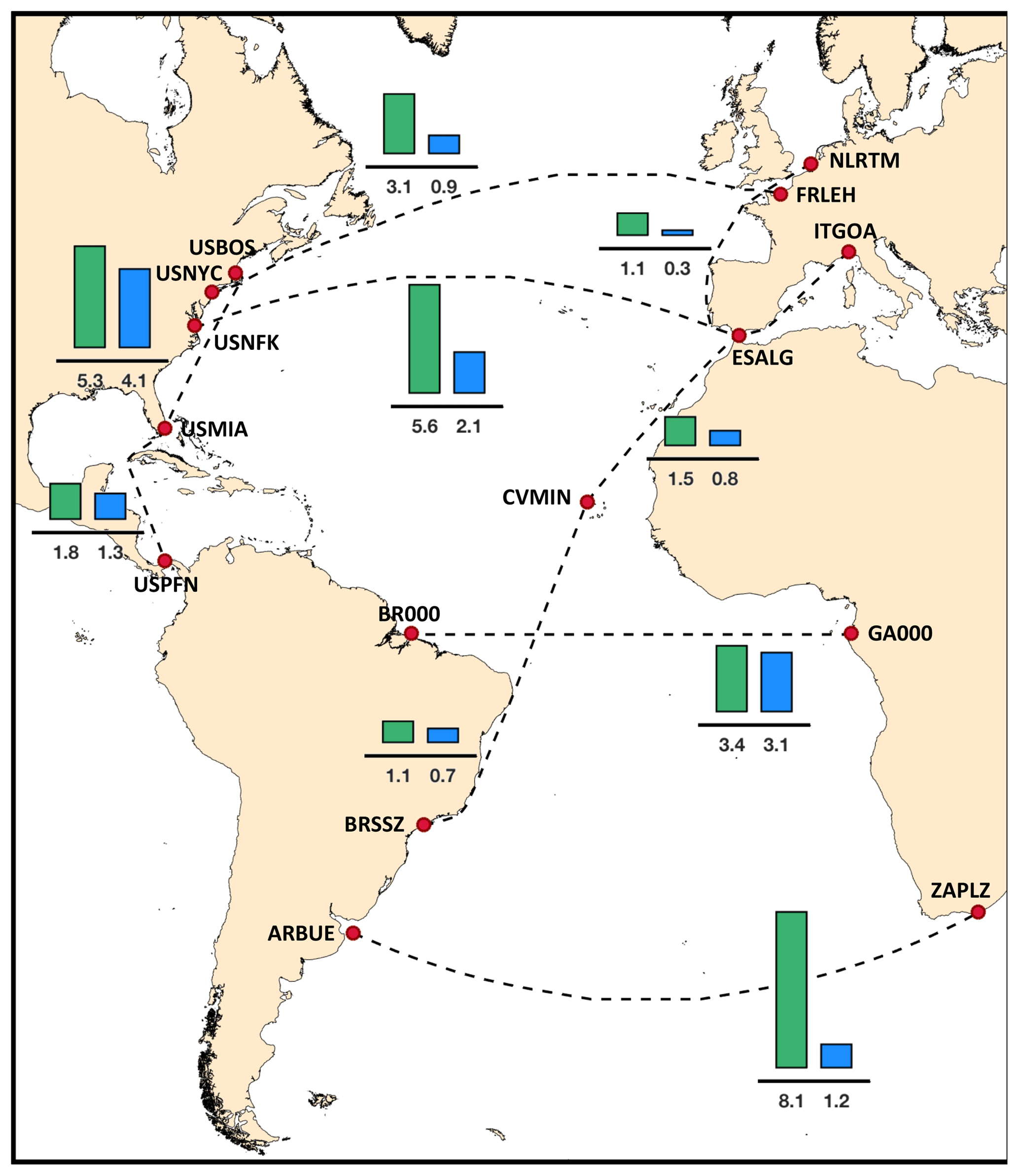
Figure 11Mean relative EEOI savings (%) for several routes in the Atlantic Ocean. The values displayed in the vertical bars refer to the annual average of the mean savings for the return voyages (i.e. mean values along the rows of Fig. 10) sailed along the optimal tracks of cw type. The green bars refer to total savings, or , while the blue bars refer to the ocean currents contribution, or .
Table 7Database of routes. Lg is the length of the geodetic track on the graph. Δ is a shortcut for the EEOI saving. The 〈⋅〉 operator denotes the annual mean. The is the mean annual value of the standard deviation. Corresponding values are given (in %). The second header line specifies the type of tracks. The other columns contain the number of tracks NE with intentional speed reduction and the maximum percent fraction of track waypoints affected (WP) – for the w type this figure is always 0 except for the ZAPLZ–ARBUE route, where it reads 1(0.4). The maximum rate of turn ROTM (), the number of non-FIFO edges (neither of them is along the optimal track), and the Pearson coefficient RP between T* and L are shown. The DOF varies from more than 5.4×10⁸ of the ARBUE–ZAPLZ to about 2.5×10⁷ of the USBOS–USMIA.
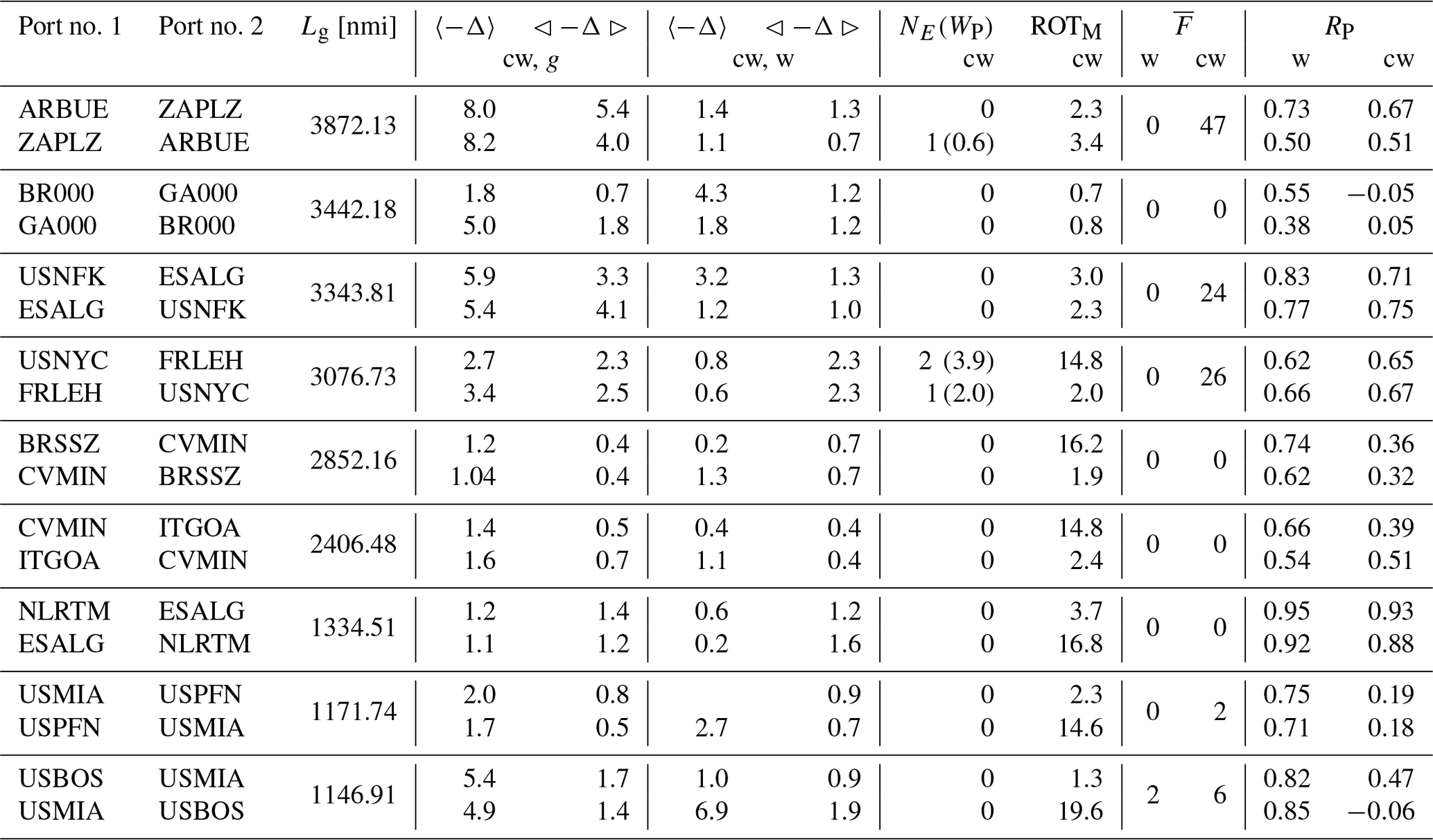
Route-specific results are discussed in the following paragraphs. In the Supplement of this paper, related figures are published, and the web application for interactive exploration is available at http://www.atlantos-visir.com/ (last access: 12 July 2019). The application allows for zooming in on optimal tracks, checking their capacity in landmass avoidance, and obtaining the EEOI savings compared to the least-distance track.
4.5.1 Buenos Aires to Port Elizabeth
The geodetic track is bent southwards in the Mercator projection. The (Northern Hemisphere) winter tracks are closer to the geodetic track, while summer tracks exhibit greater diversions. This route is characterised by the highest impact of waves on energy efficiency savings. This can be ascribed to the strength of the Antarctic circumpolar winds, causing large waves in the Southern Ocean (Lu et al., 2017). The role of currents in EEOI savings is instead about 1 %, with a stronger contribution from the Benguela Current for eastbound crossings. This is generally due to the avoidance of the Agulhas Current past Cape Town.
4.5.2 Equator route
This route does not join any major harbour and is just meant for sampling the equatorial currents. In fact, the w-type optimal tracks are quite close to being an arc of the Equator. Nearly all of the optimal eastbound cw-type tracks instead divert up to 5∘ N. This is for skipping the North Equatorial Current and exploiting, wherever possible, the Equatorial Counter Current. However, the westbound tracks make use of the North Brazil Current, diverting either N or S of the Equator by up to 3∘.
4.5.3 Norfolk to Algeciras
This is the route discussed in the featured case study of Sect. 4.3. As this confirms, the route is affected, to an appreciable extent, by both waves and currents. The Gulf Stream significantly increases the efficiency of the eastbound crossings, and a clear seasonality of the EEOI savings is observed.
4.5.4 New York City to Le Havre
At their western edge, these optimal tracks tend to sail inshore of Nova Scotia and Newfoundland and in some cases even in the Gulf of Saint Lawrence (Canada), also experiencing the effect of the Labrador Current. This solution may not be viable in practice for two reasons. First, in winter, sea ice can extend several tens of miles off the coastline. Second, coastal Canada is part of the Emission Control Areas (ECAs; IMO, 2009a), which may cause vessels to sail normally to the shoreline to leave the ECA more quickly. Neither effects are presently modelled within VISIR.
4.5.5 Santos to Mindelo
This route spans across both hemispheres. The optimal tracks of w type do not significantly differ from the geodetic track, with the Equator being crossed at about 31∘ W. However, as ocean currents are also accounted for (cw type), the crossing occurs within the 33–29∘ W band, depending on the actual strength of the North Brazil Current.
4.5.6 Mindelo to Genoa
This route connects the Atlantic Ocean to the Mediterranean Sea. In both sailing directions, it is dominated by waves. The tracks of cw type are influenced by both the Atlantic jet past Gibraltar and the Canary Current. They approach the energy-efficient region (Sect. 4.4.3), particularly at the end of summer and in autumn. Topologically, they can sail very close to the shores of Morocco and Western Sahara.
4.5.7 Rotterdam to Algeciras
This route links the major harbour of the Atlantic (Table 6) to the Mediterranean. The optimal tracks only slightly divert from the geodetic one, sailing close to some of the major western European capes (Gibraltar, Cabo da Roca, Finisterre, northwestern Brittany, and the Strait of Dover). On just one date (1 February 2017), the optimal track sails several tens of miles inshore into the Bay of Biscay whether ocean currents are accounted for or not. This is due to the activation of the parametric roll safety constraint (Sect. 2.5.2), as the encounter period of waves is about half the natural roll period TR of the vessel (Table 4). This occurs only for the track leaving from Rotterdam, as waves are encountered at a lower frequency on the other sailing direction.
4.5.8 Miami to Panama
The spatial variability in this route is dominated by currents, as waves from subpolar lows are not relevant in the Caribbean region. The bundle shows a waist W of Cuba ( N, W), a point through which all optimal tracks but one sail. In fact, on 11 September 2017, the track leaving Miami was affected by large waves in the Gulf of Mexico generated by the transit of Hurricane Irma (https://en.wikipedia.org/wiki/2017_Atlantic_hurricane_season, last access: 12 July 2019). Here, the sea state, together with a local intensification of the GS in the Straits of Florida, leads to an optimal track sailing E of Cuba.
4.5.9 Boston to Miami
This route is heavily influenced by the Florida current. The northbound tracks tend to align with the ocean flow. The southbound tracks (sailing against the main flow) split into two sub-bundles, W and E of the Florida current. The western sub-bundle is populated by mainly winter tracks. In fact, these tracks sail more inshore, avoiding the rough ocean state and thus reducing the speed loss in waves.
The VISIR ship-routing model and code have been updated to version 1-b. Optimal tracks can now be computed in the presence of both time-dependent ocean currents and waves. Vessel interaction with currents is described in terms of new equations which are validated by means of an analytical benchmark. To represent vessel courses with a higher degree of accuracy, the previous model version has been improved with respect to the capacity of computing graphs of a higher order of connectivity, thus accounting also for the shoreline. The computational cost and memory allocation of the new model version is also assessed, and the inclusion of ocean currents leads to a total CPU time overhead not exceeding 30 % for realistic computations (Fig. 3c).
While the code of VISIR-1.a was tested through its operational implementation in the Mediterranean Sea (Mannarini et al., 2016b), the robustness of VISIR-1.b has been proven through the computation of more than 2500 tracks via the same model code version, spanning nearly all subdomains of the Atlantic Ocean.
Several routes are considered, and the variability in the optimal tracks is mapped across a full calendar year (2017). Both spatial and kinematical variabilities in the tracks are accounted for through various types of diagrams. The optimal exploitation of ocean currents may in some cases lead to average speeds greater than the maximum vessel speed in calm water (see Figs. 8–9). Finally, a standard voyage efficiency indicator (EEOI; introduced by the International Maritime Organization) is used to highlight the contribution of ocean currents and waves to the efficiency of the voyages. In some cases, EEOI relative savings were in excess of 5 % (annual averages) and 10 % (monthly averages; see Figs. 10–11). However, the intra-monthly, seasonal, and regional dependence of these results is quite high, and this study provides one of the first attempts to quantify it. It should also be noted that these results depend on the actual parametrisation of wave-added resistance, which are still formally the same as those of Mannarini et al. (2016a). These quantitative assessments of EEOI savings through path optimisation may be considered in terms of the ongoing discussion at the IMO level about comparing the effectiveness of several proposed methods for vessel emission savings (IMO, 2018a).
Furthermore, the analysis of the track dataset is simplified by means of metrics such as the optimal track duration and length, their Pearson's correlation coefficient, and the maximum rate of turn of vessel heading. The correlation coefficient carries a signature of ocean currents, which tend to make optimal track duration and its length less correlated to each other. Furthermore, the approximation of a FIFO network (Sect. 2.4) is monitored and found to be satisfied to a great extent (Table 7). Vessel EOT is allowed to vary (Sect. 2.5.2), and the computation of the EEOI savings accounts for this. However, intentional speed reduction is found to be a rare choice of the optimisation algorithm.
We regard the main computational limitation of VISIR-1.a and VISIR-1.b to be its requirement on computer RAM allocation (Sect. 3.2.2). The code still requires the preparation of all the time-dependent graph edge weights, ahead of the shortest path computations. This presently affects the capacity to describe the environmental state surrounding the vessel. For example, in this work, we averaged 3-hourly wave fields to daily averages (Sect. 4.1.4) but neglected other wave spectrum components (such as swell), and we did not account for Stokes's drift contribution to the flow advecting the vessel.
However, it should be noted that a more realistic representation of the marine state is likely to correspond to a more accurate description of the mechanical interaction between it and the vessel, particularly with reference to speed loss in waves and wind (Tsujimoto et al., 2013; Bertram and Couser, 2014). The presence of sea ice and ECA zones may also affect the optimal tracks. While the former effect may decrease in significance due to global warming, the latter has the potential to shape increasingly more coastal traffic as the new IMO global cap on sulfur contents enters into force (IMO, 2016). Developing the representation of some of these model components is planned for future VISIR versions (e.g. in the frame of the newly started GUTTA project, http://bit.ly/guttaproject, last access: 12 July 2019) and will pave the way for end-to-end model evaluation exercises with respect to actually sailed trajectories.
VISIR-1.b is coded in MATLAB 2016a, which was used on both the workstation (Mac OS 10.11.6 El Capitan; used for the performance analysis of Sect. 3.2) and the cluster (Unix CentOS release 6.9 “Final”, used for the mass production of Sect. 4). In addition, the MEXCDF library is required. The list of all third-party MATLAB functions is provided along with the VISIR-1.b release. The source code of VISIR-1.b is released with an LGPL licence at https://doi.org/10.5281/zenodo.2563074 (Mannarini and Carelli, 2019a).
The additional figures referred to in Sect. 4.5 are part of the Supplement. Support data assets for the figures and tables of this paper can be found at https://doi.org/10.5281/zenodo.3258177 (Mannarini and Carelli, 2019b).
Animations for each of the panels of Fig. 7 can be found at https://av.tib.eu/series/560/gmdd+18 (last access: 12 July 2019; https://doi.org/10.5446/38218, Mannarini and Carelli, 2019c, https://doi.org/10.5446/38483, Mannarini and Carelli, 2019d, https://doi.org/10.5446/38484, Mannarini and Carelli, 2019e, https://doi.org/10.5446/38482, Mannarini and Carelli, 2019f).
The most relevant changes of VISIR-1.b described in this paper are listed in Table A1. The list does not include other minor code updates, for which we refer to the release notes of the new model version (see Code and data availability).
Table A1List of main code changes of VISIR-1.b with respect to VISIR-1.a, with indication of their use within this paper.
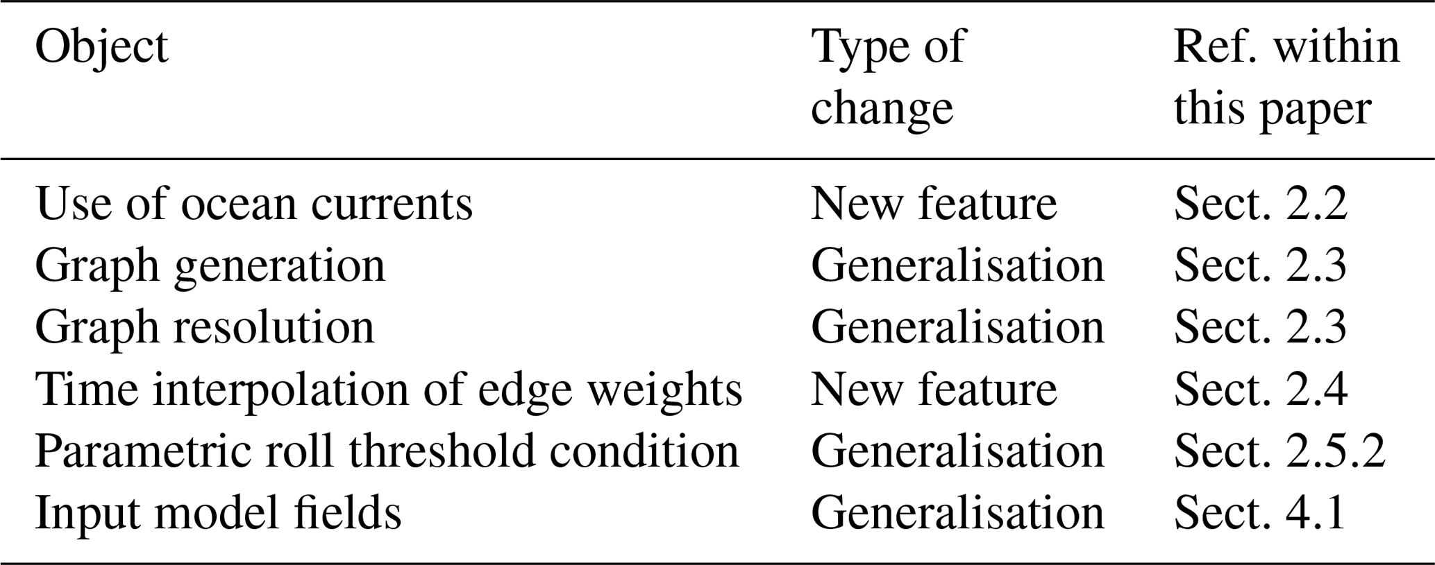
In order to head as prescribed by the optimal track, the ship has to be manoeuvred (e.g. acting on rudder and/or lateral thrusters; Bertram, 2000). The rudder is handled via a hydraulic device that converts pressure into a mechanical action to move the rudder (https://www.wartsila.com/encyclopedia/term/rudder-actuator, last access: 12 July 2019). In order to implement the prescribed EOT, the high-level order from the control bridge is transmitted through potentiometers (https://www.kwantcontrols.com/product/systems/integrated-telegraph-system/, last access: 12 July 2019) to the main engines (and possibly also to other components of the propulsion system, such as clutches, a gearbox, and a controllable pitch propeller; see Harvald, 1992).
Motions of the bottom layer (rudder and main engine), as related to electromechanical devices, should occur on a much shorter timescale (probably seconds to a few minutes) than the top-level controls needed for implementing the optimal track (requiring changes of the order of minutes – see ROTM in Table 7 – to hours – see Fig. 6). Thus, a routing system must ensure that the top-level control requires feasible manoeuvers (e.g. in Sect. 4.3.2 we check that maximum vessel rate of turn ROTM is in an acceptable range; other feasibility criteria are defined in IMO, 2002). If this condition is satisfied, it should be possible, for the sake of computation of the optimal track, to safely ignore the temporal dynamics of the underlying actuation level (Techy, 2011). On the other hand, if the actuator timescale were comparable to the time over which heading and EOT changes should take place, the hypothesis of top–bottom-level separation would be invalid. We presume that this is much less likely to occur in open-sea navigation (which is the subject of the present paper) than, for example, during harbour operations. However, on-board data would be needed for a thorough assessment of this issue.
Following Mannarini et al. (2016a), we took into consideration the fact that the VISIR graph grid may need to be redesigned, e.g. by reducing the density of grid points in open seas through the use of a non-uniform mesh. An adaptive refinement mesh (Berger and Colella, 1989) or unstructured mesh limiting the minimum angle (Shewchuk, 2002) could be another option. This would reduce the number of open-ocean edges, thereby reducing RAM allocation (see Sect. 3.2.2) and speeding up the computation of the shortest path.
In any case, to ensure navigation safety, the intersection between graph arcs and the shoreline (Sect. 2.3) needs to be verified, irrespective of the grid resolution or structure. In fact, even if the mesh is built via a tessellation, intersection with islands and boundary elements smaller than mesh elements should be checked (Legrand et al., 2000). For a graph of a higher order of connectivity (ν≫1) this is even more challenging. Such a check on shoreline intersection can easily represent a significant computational cost (De Berg et al., 1997). In order to perform it effectively, it is crucial to be able to find indices of graph elements next the shoreline. On a regular grid, this operation can be carried out in 𝒪(M) time (M is the number of shoreline elements), irrespective of the size of the maritime domain (and we exploited this in the first step of the algorithm described in Sect. 2.3). Instead, on a random or non-regular mesh, a 𝒪(M⋅n) time would be required by a linear search (n is here the number of arcs of the graph). To speed up the search on a non-regular mesh, a preliminary node indexing can be computed. With a k-dimensional tree, an additional 𝒪(n log(n)) time for tree construction and, on average, 𝒪(M⋅log(n)) for querying would be needed (Bentley, 1975). This is in excess of the 𝒪(M) estimate for corresponding step (see first step in Sect. 2.3) in the present VISIR graph creation algorithm.
Thus, at this stage we still use a regular grid which enables a relatively quick and easy graph computation at the cost of a longer path computing time. This is not critical, given the non-operational functioning of VISIR for the present exercise. In future model versions, also depending on coding options, domain, and type of application, we may reconsider this choice.
Since the VISIR solution is based on Dijkstra's algorithm, it is not just guaranteed to be exact; its performance (for a given route and vessel departure date) is stable over subsequent runs. This is a difference to evolutionary (EA) and, generally speaking, to heuristic-based algorithms. For that class of algorithm, both the quality and the computational cost of the solution may vary over subsequent runs, as they are driven by random effects. The issue of randomness can be mitigated by statistical averaging over many simulations. However, a more fundamental issue is that, as clearly stated in Eiben and Smith (2003), the performance of an EA should be assessed in terms of both efficiency (CPU time) and effectiveness (quality of the solution). Furthermore, even for a specific EA and EA implementation, performance may vary with tuning. Tuning refers to specifying values for the algorithm parameters, such as the “mutation rate”. Tuning may affect both EA performance and robustness (Eiben and Smith, 2003). Apart from the particular features of EA, comparing the performance of VISIR with other ship-routing systems is also hampered by the facts mentioned in Sect. 1.1. These need to be overcome in dedicated collaborative efforts, as we did in Mannarini et al. (2019a). We are open to replicating that approach for EA-based ship-routing models, e.g. the ant-colony algorithm described in Tsou and Cheng (2013) or the multi-objective EA reported in Szlapczynska (2015).
The supplement related to this article is available online at: https://doi.org/10.5194/gmd-12-3449-2019-supplement.
GM worked on conceptualisation, methodology, software, supervision, validation, visualisation, writing, reviewing, and editing. LC contributed to methodology (Sect. 2.3), software development, and visualisation.
Links MT worked together with CMCC to run the operational service (http://www.visir-nav.com/, last access: 12 July 2019) for which both free and premium versions exist; the authors declare no competing interests with these. Furthermore, the term VISIR is a trademark of CMCC and is registered at EUIPO: https://euipo.europa.eu/ (last access: 12 July 2019).
Research results are not to be used for navigation. Neither the authors nor CMCC are liable for any damage or loss to assets or persons deriving from use of tracks computed by VISIR.
We would like to thank Nadia Pinardi (University of Bologna) for her advice on the validation of the model, Fabio Montagna (CMCC) for consultancy on graph indexing, and Florian Aendekerk (Compagnie Maritime Belge) for providing realistic parameters of a container ship.
This research has been supported by the European Commission project AtlantOS (grant no. 633211).
This paper was edited by David Ham and reviewed by two anonymous referees.
Aendekerk, F.: Weather Route Optimization for Oceanic Vessels, Master's thesis, Delft University of Technology, 2018. a
Alexandersson, M.: A study of methods to predict added resistance in waves, Master's thesis, KTH Centre for Naval Architecture, 2009. a
Almeida, J., Silvestre, C., and Pascoal, A.: Cooperative control of multiple surface vessels in the presence of ocean currents and parametric model uncertainty, Int. J. Robust Nonlin., 20, 1549–1565, 2010. a
Aouf, L. and Lefevre, J.-M.: On the assimilation of the ASAR L2 wave spectra in the operational wave model MFWAM, in: SeaSAR 2012, vol. 709, 2013. a
Apel, J. R.: Principles of ocean physics, vol. 38, Academic Press, 1987. a, b
Bazari, Z. and Longva, T.: MEPC 63/INF.2 (Annex) assessment of imo mandated energy efficiency measures for international shipping. Technical report, International Maritime Organization, London, UK, 2011. a
Belenky, V., Bassler, C. G., and Spyrou, K. J.: Development of Second Generation Intact Stability Criteria, Tech. rep., DTIC Document, 2011. a, b, c
Bentley, J. L.: Multidimensional Binary Search Trees Used for Associative Searching, Commun. ACM, 18, 509–517, https://doi.org/10.1145/361002.361007, 1975. a
Berger, M. J. and Colella, P.: Local adaptive mesh refinement for shock hydrodynamics, J. Comput. Phys., 82, 64–84, 1989. a
Berline, L., Testut, C.-E., Brasseur, P., and Verron, J.: Variability of the Gulf Stream position and transport between 1992 and 1999: a re-analysis based on a data assimilation experiment, Int. J. Remote Sens., 27, 417–432, 2006. a
Bertram, V.: Practical ship hydrodynamics, Elsevier, Woburn, MA, 2000. a
Bertram, V. and Couser, P.: Computational Methods for Seakeeping and Added Resistance in Waves, in: 13th International Conference on Computer and IT Applications in the Maritime Industries, Redworth, 12–14 May 2014, edited by: Volker, B., Technische Universität Hamburg-Harburg, 8–16, 2014. a
Bertsekas, D.: Network Optimization: Continuous and Discrete Models, Athena Scientific, Belmont, Mass., 02178-9998, USA, 1998. a, b, c
Bijlsma, S.: On minimal-time ship routing, PhD thesis, Delft University of Technology, 1975. a, b, c
Bijlsma, S.: Optimal ship routing with ocean current included, J. Navigation, 63, 565–568, 2010. a, b, c
Bos, M.: An Ensemble Prediction of Added Wave Resistance to Identify the Effect of Spread of Wave Conditions on Ship Performance, in: 3rd Hull Performance & Insight Conference, edited by: Bertram, V., 265–274, available at: http://data.hullpic.info/hullpic2018_redworth.pdf (last access: 12 July 2019), 2018. a
Breivik, Ø. and Allen, A. A.: An operational search and rescue model for the Norwegian Sea and the North Sea, J. Marine Syst., 69, 99–113, 2008. a
Broer, H. W.: Bernoulli's light ray solution of the brachistochrone problem through Hamilton's eyes, International Journal of Bifurcation and Chaos, 24, 1440009, https://doi.org/10.1142/S0218127414400094, 2014. a
Chang, Y.-C., Tseng, R.-S., Chen, G.-Y., Chu, P. C., and Shen, Y.-T.: Ship routing utilizing strong ocean currents, J. Navigation, 66, 825–835, 2013. a, b
Cheung, J. C. H.: Flight planning: node-based trajectory prediction and turbulence avoidance, Meteorol. Appl., 25, 78–85, https://doi.org/10.1002/met.1671, 2017. a
Clementi, E., Oddo, P., Drudi, M., Pinardi, N., Korres, G., and Grandi, A.: Coupling hydrodynamic and wave models: first step and sensitivity experiments in the Mediterranean Sea, Ocean Dynam., 67, 1293–1312, https://doi.org/10.1007/s10236-017-1087-7, 2017. a
De Berg, M., Van Kreveld, M., Overmars, M., and Schwarzkopf, O.: Computational geometry, in: Computational geometry, Springer, 1–17, 1997. a
Diestel, R.: Graph Theory, Springer-Verlag, available at: http://diestel-graph-theory.com/ (last access: 12 July 2019), 2005. a
Dijkstra, E. W.: A note on two problems in connexion with graphs, Numer. Math., 1.1, 269–271, 1959. a
Dubins, L. E.: On curves of minimal length with a constraint on average curvature, and with prescribed initial and terminal positions and tangents, Am. J. Math., 79, 497–516, 1957. a
Eiben, A. E. and Smith, J. E.: Introduction to evolutionary computing, vol. 53, Springer, 2003. a, b
Foschini, L., Hershberger, J., and Suri, S.: On the complexity of time-dependent shortest paths, Algorithmica, 68, 1075–1097, 2014. a
Fossen, T. I.: How to incorporate wind, waves and ocean currents in the marine craft equations of motion, IFAC P. Ser., 45, 126–131, 2012. a, b
Fossen, T. I., Pettersen, K. Y., and Galeazzi, R.: Line-of-sight path following for dubins paths with adaptive sideslip compensation of drift forces, IEEE T. Contr. Syst. T., 23, 820–827, 2015. a
Fu, L.-L. and Smith, R. D.: Global ocean circulation from satellite altimetry and high-resolution computer simulation, B. Am. Meteorol. Soc., 77, 2625–2636, 1996. a
Fujii, M., Hashimoto, H., and Taniguchi, Y.: Analysis of satellite AIS Data to derive weather judging criteria for voyage route selection, TransNav: International Journal on Marine Navigation and Safety of Sea Transportation, 11, 271–277, https://doi.org/10.12716/1001.11.02.09, 2017. a
Fujiwara, T., Ueno, M., and Ikeda, Y.: Cruising performance of a large passenger ship in heavy sea, in: The Sixteenth International Offshore and Polar Engineering Conference, International Society of Offshore and Polar Engineers, 2006. a
Gerritsma, J. and Beukelman, W.: Analysis of the resistance increase in waves of a fast cargo ship, International Shipbuilding Progress, 19, 285–293, 1972. a
Harvald, S. A.: Resistance and propulsion of ships, Krieger Publishing Company, 1992. a
Hinwood, J. B., Blackman, D. R., and Lleonart, G. T.: Some properties of swell in the Southern Ocean, in: 18th International Conference on Coastal Engineering, 261–269, https://doi.org/10.1061/9780872623736.017, 1982. a
IMO: Resolution A.526(13) Performance Standards for Rate-Of-Turn Indicators, Tech. rep., International Maritime Organization (IMO), London, UK, 1983. a
IMO: MSC 76/23/Add.1 Resolution MSC.137(76), Annex 6 – Standards for ship manoeuvrability, Tech. rep., International Maritime Organization, London, UK, 2002. a
IMO: MSC.1/Circ.1228 Revised guidance to the Master for avoiding dangerous situations in adverse weather and sea conditions, Tech. rep., International Maritime Organization, London, UK, 2007. a, b
IMO: MSC.1/Circ.1281 Explanatory notes to the international code on intact stability, Tech. rep., International Maritime Organization, London, UK, 2008. a
IMO: MEPC 59/65/5 Interpretations of, and amendments to, MARPOL and related instruments, Tech. rep., International Maritime Organization, London, UK, 2009a. a
IMO: MEPC.1/Circ.684 Guidelines for voluntary use of the ship Energy Efficiency Operational Indicator (EEOI), Tech. rep., International Maritime Organization, London, UK, 2009b. a, b
IMO: MEPC 59/INF.10 (Annex) “Second IMO GHG Study 2009”, Technical report, International Maritime Organization, London, UK, 2009c. a
IMO: MEPC 67/INF.3 (Annex) “Third IMO GHG Study 2014”, Technical report, International Maritime Organization, London, UK, 2014. a
IMO: MEPC.176(58) Amendments to MARPOL Annex VI, Tech. rep., International Maritime Organization, London, UK, 2016. a
IMO: MEPC 73/WP5 Report of the fourth meeting of the Intersessional Working Group on Reduction of GHG emissions from ships (ISWG-GHG 4), Tech. rep., International Maritime Organization, London, UK, 2018a. a
IMO: MEPC.304(72) Initial IMO strategy on reduction of GHG emissions from ships, Tech. rep., International Maritime Organization, London, UK, 2018b. a
IMO: SDC 5/J/7 Finalization of second generation intact stability criteria, Tech. rep., International Maritime Organization, London, UK, 2018c. a
IPCC: Global Warming of 1.5 deg, Tech. rep., WMO, UNEP, available at: http://ipcc.ch/report/sr15/ (last access: 12 July 2019), 2018. a
Jameson, A. and Vassberg, J. C.: Studies of alternative numerical optimization methods applied to the brachistochrone problem, Computational Fluid Dynamics Journal, 9, 281–296, 2000. a
JRC and PBL: Emission Database for Global Atmospheric Research (EDGAR), Tech. rep., European Commission, available at: http://edgar.jrc.ec.europa.eu/overview.php?v=CO2ts1990-2015 (last access: 12 July 2019), 2016. a
Kang, D., Curchitser, E. N., and Rosati, A.: Seasonal variability of the Gulf Stream kinetic energy, J. Phys. Oceanogr., 46, 1189–1207, 2016. a
Komen, G. J., Cavaleri, L., Donelan, M., Hasselmann, K., Hasselmann, S., and Janssen, P.: Dynamics and modelling of ocean waves, Dynamics and Modelling of Ocean Waves, edited by: Komen, G. J., Cavaleri, L., Donelan, M., Hasselmann, K., Hasselmann, S., and Janssen, P. A. E. M., 554 pp., ISBN 0521577810, Cambridge, UK, Cambridge University Press, August 1996, p. 554, 1996. a
Legrand, S., Legat, V., and Deleersnijder, E.: Delaunay mesh generation for an unstructured-grid ocean general circulation model, Ocean Modell., 2, 17–28, 2000. a
Likhachev, M., Ferguson, D. I., Gordon, G. J., Stentz, A., and Thrun, S.: Anytime Dynamic A*: An Anytime, Replanning Algorithm, in: ICAPS, 262–271, 2005. a
Lloyd's: Top 100 – Container Ports 2017, Tech. rep., Informa UK Ltd, available at: https://maritimeintelligence.informa.com/content/top-100-success (last access: 12 July 2019), 2018. a
Lo, H. K. and McCord, M. R.: Routing through dynamic ocean currents: General heuristics and empirical results in the gulf stream region, Transport. Res. B-Meth., 29, 109–124, 1995. a, b
Lo, H. K. and McCord, M. R.: Adaptive ship routing through stochastic ocean currents: General formulations and empirical results, Transport. Res. A-Pol., 32, 547–561, 1998. a
Lolla, T., Lermusiaux, P. F., Ueckermann, M. P., and Haley Jr., P. J.: Time-optimal path planning in dynamic flows using level set equations: theory and schemes, Ocean Dynam., 64, 1373–1397, 2014. a
Loria, A., Fossen, T. I., and Panteley, E.: A separation principle for dynamic positioning of ships: theoretical and experimental results, IEEE T. Contr. Syst. T., 8, 332–343, 2000. a
Lu, L.-F., Sasa, K., Sasaki, W., Terada, D., Kano, T., and Mizojiri, T.: Rough wave simulation and validation using onboard ship motion data in the Southern Hemisphere to enhance ship weather routing, Ocean Eng., 144, 61–77, 2017. a
Lu, R., Turan, O., Boulougouris, E., Banks, C., and Incecik, A.: A semi-empirical ship operational performance prediction model for voyage optimization towards energy efficient shipping, Ocean Eng., 110, 18–28, https://doi.org/10.1016/j.oceaneng.2015.07.042, 2015. a
Luenberger, D.: Introduction to dynamic systems: theory, models, and applications, Wiley, New York, Chicester, Brisbane, Toronto, 1979. a, b
Lumpkin, R., Treguier, A.-M., and Speer, K.: Lagrangian eddy scales in the northern Atlantic Ocean, J. Phys. Oceanogr., 32, 2425–2440, 2002. a
Madec, G.: NEMO reference manual, ocean dynamic component: NEMO-OPA, Note du pôle de modélisation, Institut Pierre Simon Laplace, France, 2008. a
MANDieselTurbo: Basic Principles of Ship Propulsion, Tech. rep., MANDieselTurbo, Augsburg, Germany, 2011. a
Mannarini, G. and Carelli, L.: ISIR-1.b ship routing model (Version 1.00), Zenodo, https://doi.org/10.5281/zenodo.2563074, 2019a. a
Mannarini, G. and Carelli, L.: Support Data Assets for Figures and Tables in gmd-2018-292 (Geosci. Model Dev.) (Version 1.05) [Data set], Zenodo, https://doi.org/10.5281/zenodo.3258177, 2019b. a
Mannarini, G. and Carelli, L.: Optimal tracks for USNFK-ESALG route in 2017, accounting for CMEMS waves, https://doi.org/10.5446/38218, 2019c. a
Mannarini, G. and Carelli, L.: Optimal tracks for USNFK-ESALG route in 2017, accounting for both CMEMS waves and ocean currents, https://doi.org/10.5446/38483, 2019d. a
Mannarini, G. and Carelli, L.: Optimal tracks for ESALG-USNFK route in 2017, accounting for CMEMS waves, https://doi.org/10.5446/38484, 2019e. a
Mannarini, G. and Carelli, L.: Optimal tracks for ESALG-USNFK route in 2017, accounting for both CMEMS waves and ocean currents, https://doi.org/10.5446/38482, 2019f. a
Mannarini, G., Lecci, R., and Coppini, G.: Introducing sailboats into ship routing system VISIR, in: 6th International Conference on Information, Intelligence, Systems and Applications (IISA 2015), IEEE-Xplore, 1–6, https://doi.org/10.1109/IISA.2015.7387962, 2015. a
Mannarini, G., Pinardi, N., Coppini, G., Oddo, P., and Iafrati, A.: VISIR-I: small vessels – least-time nautical routes using wave forecasts, Geosci. Model Dev., 9, 1597–1625, https://doi.org/10.5194/gmd-9-1597-2016, 2016. a, b, c, d, e, f, g, h, i, j, k, l, m, n, o, p, q, r, s, t
Mannarini, G., Turrisi, G., D'Anca, A., Scalas, M., Pinardi, N., Coppini, G., Palermo, F., Carluccio, I., Scuro, M., Cretì, S., Lecci, R., Nassisi, P., and Tedesco, L.: VISIR: technological infrastructure of an operational service for safe and efficient navigation in the Mediterranean Sea, Nat. Hazards Earth Syst. Sci., 16, 1791–1806, https://doi.org/10.5194/nhess-16-1791-2016, 2016b. a, b
Mannarini, G., Subramani, D., Lermusiaux, P., and Pinardi, N.: Graph-Search and Differential Equations for Time-Optimal Vessel Route Planning in Dynamic Ocean Waves, IEEE T. Intell. Transp., accepted, 2019a. a, b, c, d
Mannarini, G., Carelli, L., Zissis, D., Spiliopoulos, G., and Chatzikokolakis, K.: Preliminary inter-comparison of AIS data and optimal ship tracks, TransNav, 13, 53–61, https://doi.org/10.12716/1001.13.01.04, 2019. a
Maximenko, N., Hafner, J., and Niiler, P.: Pathways of marine debris derived from trajectories of Lagrangian drifters, Mar. Pollut. Bull., 65, 51–62, 2012. a
Meehl, G. A.: Characteristics of surface current flow inferred from a global ocean current data set, J. Phys. Oceanogr., 12, 538–555, 1982. a
Minobe, S., Miyashita, M., Kuwano-Yoshida, A., Tokinaga, H., and Xie, S.-P.: Atmospheric response to the Gulf Stream: Seasonal variations, J. Climate, 23, 3699–3719, 2010. a
Morin, D.: The Lagrangian Method, Tech. rep., Harvard, available at: http://www.people.fas.harvard.edu/~djmorin/chap6.pdf (last access: 12 July 2019), 2007. a
Munk, W. H.: Origin and generation of waves, Tech. rep., SCRIPPS Institution of Ocenography, La Jolla, 1951. a
Newman, J. N.: Marine hydrodynamics, MIT press, Cambridge, Massachusetts and London, England, 1977. a
Orda, A. and Rom, R.: Shortest-path and Minimum-delay Algorithms in Networks with Time-dependent Edge-length, J. ACM, 37, 607–625, 1990. a, b
Pascual, A., Faugère, Y., Larnicol, G., and Traon, P. L.: Improved description of the ocean mesoscale variability by combining four satellite altimeters, Geophys. Res. Lett., 33, L02611, https://doi.org/10.1029/2005GL024633, 2006. a
Perakis, A. and Papadakis, N.: Minimal Time Vessel Routing in a Time-Dependent Environment, Transportation Science, 23, 266–276, 1989. a
Pereira, A. A., Binney, J., Hollinger, G. A., and Sukhatme, G. S.: Risk-aware Path Planning for Autonomous Underwater Vehicles using Predictive Ocean Models, J. Field Robot., 30, 741–762, 2013. a
Pinardi, N., Zavatarelli, M., Adani, M., Coppini, G., Fratianni, C., Oddo, P., Simoncelli, S., Tonani, M., Lyubartsev, V., Dobricic, S., and Bonaduce, A.: Mediterranean Sea large-scale low-frequency ocean variability and water mass formation rates from 1987 to 2007: a retrospective analysis, Prog. Oceanogr., 132, 318–332, 2015. a
Pontryagin, L., Boltyianskii, V., Gamkrelidze, R., and Mishchenko, E.: The Mathematical Theory of Optimal Processes, vol. 4, Interscience, New York, London, Paris, Montreux, Tokyo, Gordon and breach science publishers Edn., 1962. a
Richardson, P. L.: Drifting in the wind: leeway error in shipdrift data, Deep-Sea Res. Pt. I, 44, 1877–1903, 1997. a, b, c
Robinson, A., Sellschopp, J., Warn-Varnas, A., Leslie, W., Lozano, C., Jr., P. H., Anderson, L., and Lermusiaux, P.: The Atlantic Ionian Stream, J. Marine Syst., 20, 129–156, https://doi.org/10.1016/S0924-7963(98)00079-7, 1999. a
Roquet, F., Wunsch, C., Forget, G., Heimbach, P., Guinet, C., Reverdin, G., Charrassin, J.-B., Bailleul, F., Costa, D. P., Huckstadt, L. A., Goetz, K. T., Kovacs, K. M., Lydersen, C., Biuw, M., Nøst, O. A., Bornemann, H., Ploetz, J., Bester, M. N., McIntyre, T., Muelbert, M. C., Hindell, M. A., McMahon, C. R., Williams, G., Harcourt, R., Field, I. C., Chafik, L., Nicholls, K. W., Boehme, L., and Fedak, M. A.: Estimates of the Southern Ocean general circulation improved by animal-borne instruments, Geophys. Res. Lett., 40, 6176–6180, 2013. a
Sandery, P. A. and Sakov, P.: Ocean forecasting of mesoscale features can deteriorate by increasing model resolution towards the submesoscale, Nat. Commun., 8, 1566, https://doi.org/10.1038/s41467-017-01595-0, 2017. a
She, J., Allen, I., Buch, E., Crise, A., Johannessen, J. A., Le Traon, P.-Y., Lips, U., Nolan, G., Pinardi, N., Reißmann, J. H., Siddorn, J., Stanev, E., and Wehde, H.: Developing European operational oceanography for Blue Growth, climate change adaptation and mitigation, and ecosystem-based management, Ocean Sci., 12, 953–976, https://doi.org/10.5194/os-12-953-2016, 2016. a
Shewchuk, J. R.: Delaunay refinement algorithms for triangular mesh generation, Computational Geometry, 22, 21–74, 2002. a
Stentz, A.: The focussed D* algorithm for real-time replanning, in: Proceedings of the International Joint Conference on Artificial Intelligence, 95, 1652–1659, 1995. a
Subramani, D. N. and Lermusiaux, P. F.: Energy-optimal path planning by stochastic dynamically orthogonal level-set optimization, Ocean Modell., 100, 57–77, 2016. a
Szlapczynska, J.: Multi-objective weather routing with customised criteria and constraints, J. Navigation, 68, 338–354, 2015. a
Techy, L.: Optimal navigation in planar time-varying flow: Zermelo's problem revisited, Intel. Serv. Robot., 4, 271–283, 2011. a, b, c, d, e, f
Techy, L., Woolsey, C. A., and Morgansen, K. A.: Planar path planning for flight vehicles in wind with turn rate and acceleration bounds, in: 2010 IEEE International Conference on Robotics and Automation (ICRA), 3240–3245, 2010. a
Tomczak, M. and Godfrey, J. S.: Regional oceanography: an introduction, Pergamon, 1994. a
Triantafyllou, M. S. and Hover, F. S.: Maneuvering and control of marine vehicles, Department of Ocean Engineering, Massachussets Institute of Technology, Cambridge, USA, 2003. a
Tsou, M.-C. and Cheng, H.-C.: An Ant Colony Algorithm for efficient ship routing, Pol. Marit. Res., 20, 28–38, 2013. a
Tsujimoto, M., Kuroda, M., and Sogihara, N.: Development of a calculation method for fuel consumption of ships in actual seas with performance evaluation, in: ASME 2013 32nd International Conference on Ocean, Offshore and Arctic Engineering, American Society of Mechanical Engineers, V009T12A047–V009T12A047, 2013. a
UNFCCC: Adoption of the Paris Agreement, Tech. Rep. s32, United Nations Office, Geneva, 2015. a
Vratanar, B. and Saje, M.: On the analytical solution of the brachistochrone problem in a non-conservative field, Int. J. Nonlin. Mech., 33, 489–505, 1998. a
Weatherall, P., Marks, K. M., Jakobsson, M., Schmitt, T., Tani, S., Arndt, J. E., Rovere, M., Chayes, D., Ferrini, V., and Wigley, R.: A new digital bathymetric model of the world's oceans, Earth Space Sci., 2, 331–345, 2015. a
Wessel, P. and Smith, W. H.: A global, self-consistent, hierarchical, high-resolution shoreline database, J. Geophys. Res.-Sol. Ea., 101, 8741–8743, 1996. a
WMO-Secretariat: Guide to Marine Meteorological Services, WMO-No.471, WMO, available at: http://www.jcomm.info/index.php?option=com_oe&task=viewDocumentRecord&docID=19901 (last access: 12 July 2019), 2017. a
Zamuda, A. and Sosa, J. D. H.: Differential evolution and underwater glider path planning applied to the short-term opportunistic sampling of dynamic mesoscale ocean structures, Appl. Soft Comput., 24, 95–108, 2014. a, b
Zor, C. and Kittler, J.: Maritime anomaly detection in ferry tracks, in: 2017 IEEE International Conference on Acoustics, Speech and Signal Processing (ICASSP), 2647–2651, 2017. a
We refer here to a regular latitude–longitude mesh with Δg spacing, distinguishing from its projection on planar coordinates, with a constant Δy spacing and a Δx depending on latitude.
The performance could be improved to 𝒪(Nlog N) in a codification making use of binary heaps (Bertsekas, 1998).
The following shell command is used: top | grep MATLAB >> RAM-timeseries.txt.
The following MATLAB commands are used: tic and toc.
- Abstract
- Introduction
- Method
- Verification and performance
- Case studies
- Conclusions
- Code and data availability
- Video supplement
- Appendix A: List of main changes of VISIR-1.b with respect to VISIR-1.a
- Appendix B: Note on manoeuvring and actuation
- Appendix C: Note on alternative graph meshes
- Appendix D: Note on model performance comparison
- Author contributions
- Competing interests
- Disclaimer
- Acknowledgements
- Financial support
- Review statement
- References
- Supplement
- Article
(9192 KB) - Full-text XML
- Companion paper 1
- Companion paper 3
-
Supplement
(36445 KB) - BibTeX
- EndNote
- Abstract
- Introduction
- Method
- Verification and performance
- Case studies
- Conclusions
- Code and data availability
- Video supplement
- Appendix A: List of main changes of VISIR-1.b with respect to VISIR-1.a
- Appendix B: Note on manoeuvring and actuation
- Appendix C: Note on alternative graph meshes
- Appendix D: Note on model performance comparison
- Author contributions
- Competing interests
- Disclaimer
- Acknowledgements
- Financial support
- Review statement
- References
- Supplement