the Creative Commons Attribution 4.0 License.
the Creative Commons Attribution 4.0 License.
 | 21 Jan 2019
Assessing bias corrections of oceanic surface conditions for atmospheric models
Julien Beaumet
Gerhard Krinner
Michel Déqué
Rein Haarsma
Laurent Li
Future sea surface temperature and sea-ice concentration from coupled ocean–atmosphere general circulation models such as those from the CMIP5 experiment are often used as boundary forcings for the downscaling of future climate experiments. Yet, these models show some considerable biases when compared to the observations over present climate. In this paper, existing methods such as an absolute anomaly method and a quantile–quantile method for sea surface temperature (SST) as well as a look-up table and a relative anomaly method for sea-ice concentration (SIC) are presented. For SIC, we also propose a new analogue method. Each method is objectively evaluated with a perfect model test using CMIP5 model experiments and some real-case applications using observations. We find that with respect to other previously existing methods, the analogue method is a substantial improvement for the bias correction of future SIC. Consistency between the constructed SST and SIC fields is an important constraint to consider, as is consistency between the prescribed sea-ice concentration and thickness; we show that the latter can be ensured by using a simple parameterisation of sea-ice thickness as a function of instantaneous and annual minimum SIC.
- Article
(9487 KB) - Full-text XML
- BibTeX
- EndNote


Coupled climate models are the most reliable tools that we have today for large-scale climate projections, such as in the Coupled Model Intercomparison Project Phase 5 (CMIP5; Taylor et al., 2012). Regional-scale information is obtained by using these global simulations as a basis for downscaling exercises. Dynamical downscaling, as opposed to empirical statistical downscaling (Hewitson et al., 2014), is carried out either with (very) high-resolution regional climate models (RCMs) (Giorgi and Gutowski, 2016) or high-resolution atmospheric global circulation models (Haarsma et al., 2016). In both cases, information about the projected changes in sea surface conditions, such as sea surface temperatures (SST), sea-ice concentration (SIC) and sea-ice thickness (SIT), is required as a lower boundary condition for the higher-resolution models. However, SST and SIC conditions modelled by coupled atmosphere–ocean global circulation models (AOGCMs or CGCMs) show important biases for the present climate (Flato et al., 2013; Levine et al., 2013; Li and Xie, 2014; Richter et al., 2014; Stroeve et al., 2012; Zhang and Zhao, 2015). For example, it has been highlighted that most of the CMIP5 models had difficulties in reliably modelling the seasonal cycle and the trend of sea-ice extent in the Antarctic over the historical period (Turner et al., 2013). Therefore, the validity and reliability of such coupled simulations is questionable for future climate projections (e.g. the end of the 21st century), and so is their use as boundary conditions when performing dynamical downscaling of future climate projections.
Prescribing correct SST is crucial for atmospheric modelling because SST determines heat and moisture exchanges with the atmosphere (Ashfaq et al., 2011; Hernández-Díaz et al., 2017). The absence of the Pacific cold tongue bias and the reduction of the double ITCZ problem in AMIP experiments with respect to the CMIP5 model experiments(Li and Xie, 2014) shows the importance of forcing atmospheric models by SST close to the observations. For instance, improvements in the modelling of tropical cyclone activity in the Gulf of Mexico (Holland et al., 2010) and of summer precipitation in Mongolia (Sato et al., 2007) were obtained by bias correcting SST and other AOGCM outputs before using them as forcing for RCMs. At high latitudes, SIC (Krinner et al., 2008; Noël et al., 2014; Screen and Simmonds, 2010) and, in some cases, SIT (Gerdes, 2006; Krinner et al., 2010) are two additional crucial boundary conditions for atmospheric models. Krinner et al. (2014) demonstrated that for the Antarctic climate as simulated by an atmospheric general circulation model, prescribed SST and sea-ice changes have greater influence than prescribed greenhouse gas concentration changes. Large-scale average winter sea-ice extent and summer SST have been identified among the key boundary forcings for regional modelling of the Antarctic surface mass balance (Agosta et al., 2013), which is the only potentially significant negative contributor to the global eustatic sea level change over the course of the 21st century (Agosta et al., 2013; Church et al., 2013; Lenaerts et al., 2016). We note that while there is a considerable body of scientific literature on the effect of varying SST and SIC on simulated climate, very few studies focused on the role of varying SIT in atmosphere-only simulations (Gerdes, 2006; Krinner et al., 2010; Semmler et al., 2016), although air–sea fluxes in the presence of sea ice are strongly influenced by the thickness of the sea ice and the overlying snow cover. Gerdes (2006) and Krinner et al. (2010) have shown that the atmospheric response to changes in Arctic SIT can induce atmospheric signals that are of similar magnitude as those due to changes in sea-ice cover. In most atmosphere-only general circulation models (AGCMs), SIT will therefore also need to be prescribed along with SST and SIC. When SST and SIC from a coupled climate model are directly used, SIT from that same run should of course be used; however, in the case that SST and SIC from the coupled model run are bias corrected, as we strongly suggest here, we argue that SIT should be prescribed in a physically consistent manner in the atmosphere-only simulation.
In this study, we describe, evaluate and discuss different existing and new methods for the construction of bias-corrected future SST, SIC and SIT. These methods generally take into account observed oceanic boundary conditions as well as the climate change signal coming from CMIP5 AOGCM scenarios to build more reliable SST and SIC conditions for future climate, which should reduce the uncertainties when used to force future climate projections. The different methods have been evaluated using a perfect model approach and by carrying out real-case applications to observations. Applied changes in mean and variances have been investigated as well as the coherence of SIC and SST after applying bias-correction methods. The analysis of the results focuses on methods for sea ice, as the bias correction of SIC is a more complicated issue to deal with. For SIT, we propose a diagnostic using SIC following Krinner et al. (1997), and an example of its application is shown in Fig. 3. Because there were no reliable observational data sets available until recently (Kurtz and Markus, 2012; Lindsay and Schweiger, 2015), we directly evaluate diagnosed SIT against new observations. In the following, we present the bias-correction methods, the data and the evaluation methods in Sect. 2.1. The results of the evaluation are shown in Sect. 3. Because SST and SIC are bias corrected separately, Sect. 3.3 presents a few considerations about SST and SIC consistency after performing bias corrections. The results are then discussed together with general considerations on the bias correction of oceanic surface conditions in Sect. 4. Finally, we sum up our findings and draw conclusions in Sect. 5.
2.1 Data
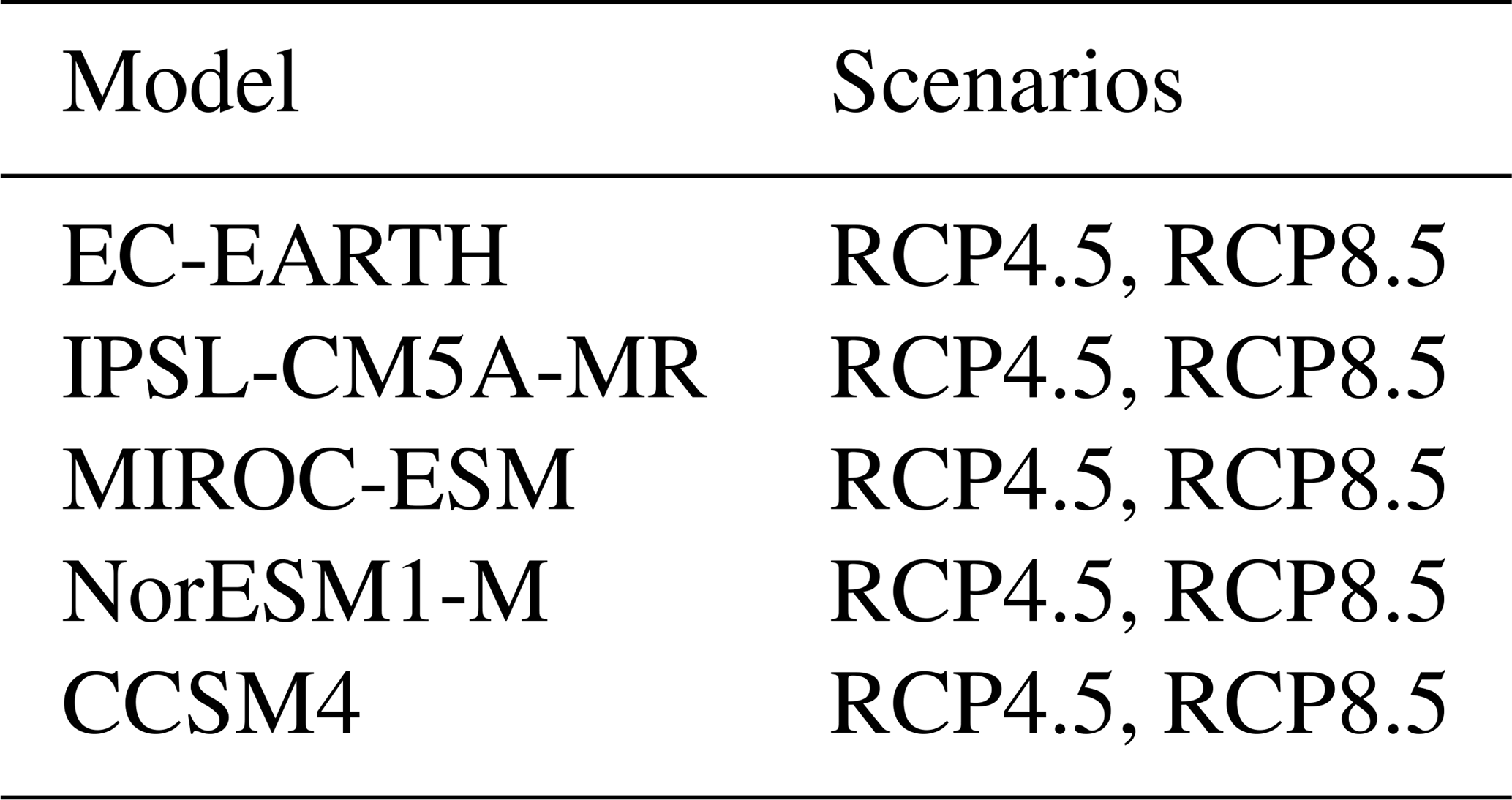
The application and validation of the methods for bias correction have been achieved using observational SST and SIC data from the Program for Climate Model Diagnosis and Intercomparison (PCMDI) that are generally used as boundary conditions for Atmospheric Model Intercomparison Project (AMIP) experiments (Taylor et al., 2000), called “PCMDI obs.” or “observations” in this paper. The AOGCM's historical and projected sea surface conditions come from CMIP5 simulations (Taylor et al., 2012). Only the first ensemble members of the historical and the Representative Concentration Pathway (RCP; Moss et al., 2010) 4.5 and 8.5 simulations have been considered. Most methods have been tested using CNRM-CM5, IPSL-CM5A-LR and HadGEM-ES coupled GCM. Data from NorESM1-M, MIROC-ESM, EC-EARTH and CCSM4 have also been used as analogue candidates in the analogue method for sea ice. Prior to any application of the bias-correction methods, AOGCM data have been bilinearly regridded onto a common regular grid. For the evaluation of the diagnosed SIT, we used the Lindsay and Schweiger (2015) data for the Arctic. For the Antarctic, in spite of recent observations with autonomous underwater vehicles by Williams et al. (2015), which tend to suggest the occurrence of thicker Antarctic sea ice than previously acknowledged, we will use the Kurtz and Markus (2012) data because of their large spatial coverage.
2.2 Sea surface temperature methods
The bias correction of simulated SST is a relatively easy and a straightforward issue to deal with. Different methods have been developed and presented in the literature. Here we re-evaluate two different frequently used methods. The first is an absolute anomaly method (e.g. Krinner et al., 2008), which consists of simply adding the SST difference for a given month from an AOGCM scenario to the climatological mean in the observations. The second is a quantile–quantile method presented in Ashfaq et al. (2011) in which for each quantile and each month, the climate change signal coming from the AOGCM scenario is added to the corresponding quantile in the observations. Presenting these well-known methods in detail is of limited interest for the main part of this paper. However, interested readers can find a more complete description of the methods in Appendix A.
2.3 Sea-ice concentration methods
SIC is more difficult to bias correct because it is a relative quantity that must be strictly bounded between 0 % and 100 %. This difficulty led some authors to neglect SIC bias correction altogether in studies with prescribed corrected future SSTs that did not specifically focus on polar regions (Hernández-Díaz et al., 2017). In this section, we present three methods: a look-up table, an iterative relative anomaly and an analogue method.
2.3.1 Look-up table method
This method has been developed at the Royal Netherlands Meteorological Institute (KNMI). It is used in Haarsma et al. (2013) and within the framework of the High Resolution Model Intercomparison Project (HighResMIP) (Haarsma et al., 2016). A regression of SIC as a function of SST is also used in the HAPPI project (Mitchell et al., 2017).
In this method, the assumption is made that SIC is a function of SST. Therefore, SSTs are ranked per 0.1 K bin and the corresponding average SIC for each temperature bin between −2 and +5 ∘C is calculated. Relations between SST and SIC have been found to be dependent on seasons and hemispheres. Therefore, using monthly mean values of SST and SIC from historical observations, look-up tables are built separately for the Arctic and the Antarctic for each calendar month (Fig. 1). Then, with the help of future SSTs, these look-up tables (LUTs) are used to retrieve future SIC.
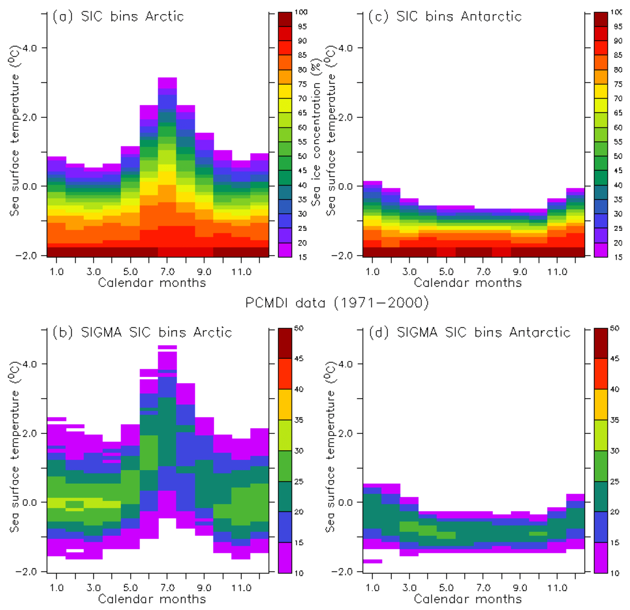
Figure 1Look-up tables (a, c) linking SST and SIC for the Arctic (a, b) and the Antarctic (c, d) built using 1971–2000 PCMDI observations and the associated uncertainty (root mean square error) in the computed SIC average (b, d).
2.3.2 Iterative relative anomaly method
Here we follow a method described by Krinner et al. (2008). It is based on relative regional sea-ice area (SIA) changes and is essentially an iterative scheme of mathematical morphology for image erosion and dilation (Haralick et al., 1987). The Arctic and the Antarctic are divided into sectors of equal longitude. In each sector, the average SIA is calculated by spatially integrating SIC. With respect to the method described in Krinner et al. (2008), we introduce the use of a quantile–quantile method to determine the targeted SIA in the bias-corrected projection. This targeted SIA is then calculated for each sector and each quantile with the help of the following equation:
In Eq. (1), SIAFut, est is the estimated projected SIA for the current month and sector, SIAObs the SIA from the observations, and SIAFut, AOGCM and SIAHist, AOGCM are the respectively computed SIAs for the corresponding quantile to the observations using SIC from a future scenario and a historical AOGCM simulation. Starting from an observed present SIC map and using the computed relative SIA change for a given sector, the decrease (increase) in SIC is then realised using an iterative process: SIC in each grid box is replaced by the minimum (maximum) SIC of all adjacent pixels (Fig. 2); the new spatially integrated SIA is calculated and the operation is repeated until the obtained change converges towards the computed targeted SIA retrieved from AOGCM-simulated sea-ice data and observations. Afterwards, the decrease–increase process is repeated on the hemisphere scale in order to ensure that the change in SIC reproduces the total hemispheric SIA change.

2.3.3 Analogue method
In this method, we divide the Arctic and the Antarctic into ns geographical sectors that correspond to different seas of the Arctic and the southern oceans; we defined ns=12 sectors for the Arctic and ns=7 sectors for the Antarctic (a map of these sectors can be seen in the Appendix, Fig. B2). For each sector and each month, the quantiles of the sea-ice extent (SIE: total area with SIC above 15 %) and the SIA are computed from SIC observations over the AMIP period. Corresponding quantile changes in SIE and SIA are computed using SICs from a CMIP5 AOGCM historical simulation and a projected scenario run. Computed quantile changes are then applied to the corresponding quantiles in the observations in order to obtain targeted future SIA and SIE for each month, quantile and sector. Then, a library of future SIC fields is built by collecting SIC observations from the AMIP period as well as SIC from CMIP5 projections. We build this library by selecting a non-exhaustive list of CMIP5 AOGCMs that represent the historical SIE annual cycle in both the Arctic and Antarctic reasonably well after consulting the literature (Shu et al., 2015; Stroeve et al., 2012; Turner et al., 2013); a list of the AOGCMs used can be found in the Appendix (Table B1). The presence of SIC maps from AOGCM projections in this library is justified by the need to take into account physically plausible future SIC distributions outside of the current observed range. Future SIC is then finally reconstructed by searching the analogue for each quantile (q), sector (s) and month (m) in the library, which is to say the SIC field that minimises the cost function C expressed by
where SIAs and SIEs are the SIA and SIE of the processed sectors of the analogue candidate from the library, SIA and SIE are the targeted projected SIE and SIA computed using the quantile–quantile method, and SIA and SIE are the maximum SIA and SIE of the processed sector. The double criterion on both SIE and SIA was introduced in order to distinguish cases in which the total SIE in a sector is similar but the average SIC is very different (and vice versa). In order to avoid issues introduced by different land masks between AOGCM and PCMDI data, we filled land grid points with sea ice using a nearest neighbour method and masked all the grid points with the same land mask built with land fraction from PCMDI data in order to compute SIEs and SIAs for each region with the same reference. Analogues are attributed without taking into account the month of the analogue candidate in the library. This allows, for instance, for the attribution of a summer sea-ice map from present observations for a future winter month reconstructed sea-ice field. For each quantile (q), month (m) and sector (s), this procedure yields a hemispheric SIC field SIC that minimises the cost function for the given sector, month and quantile. For a given month and quantile, there are thus ns hemispheric SIC fields SIC. At each grid point i, the corresponding ns SIC values are then blended using a weight function w(i, s) depending on the distance d(i, s) of that grid point to the centre of each of the sectors in order to obtain the final reconstructed SIC, SIC, for a given quantile (q) and month (m):
with
Here, dr is a reference distance of 500 km, yielding a smooth transition at the boundaries between two adjacent sectors. At the centre of a sector, this yields a weight that is very close to 1 for the relevant field that was identified as optimal for that sector and that is close to 0 for the fields identified as optimal for the other sectors; at the boundary between two sectors, the weights are typically 0.5 for the two relevant sectors and close to 0 for the others.
2.4 Sea-ice thickness method
2.4.1 Diagnosing sea-ice thickness from sea-ice concentration
As described by Krinner et al. (2010), the parameterisation of sea-ice thickness (SIT denoted hS in the following) as a function of the local instantaneous SIC f and annual minimum SIC fmin is designed to yield hS of the order of 3 m for multi-year sea ice (deemed to be dominant when the local annual minimum fraction fmin≫0), hS below 60 cm (with a stronger annual cycle) in regions where sea ice completely disappears in summer (that is, fmin=0) and intermediate values for intermediate cases:
with c1=0.2 m, c2=2.8 m and c3=2 m. This corresponds to the observed characteristics of Arctic and Antarctic sea ice, with multi-year sea ice being generally much thicker than first-year ice. The parameter c3 introduces a seasonal ice thickness variation in areas where there is a concomitant seasonal cycle of SIC. A more parsimonious formulation using only two parameters could have been designed to comply with these constraints. However, for the sake of consistency with previous work, we used the equation proposed by Krinner et al. (1997), who designed the parameterisation to allow for a fairly strong seasonal cycle of SIT also in regions with intermediate values of fmin.
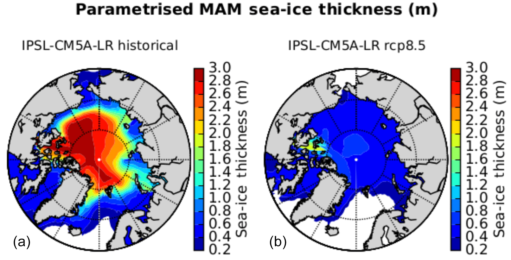
Figure 3Spring (MAM) estimated mean SIT (m) using parameterisation from Krinner et al. (1997) and IPSL-CM5A-LR SIC data from the historical run (1971–2000, a) and the RCP8.5 scenario (2071–2100, b).
2.5 Evaluation
Evaluation of the above methods is mainly achieved with a perfect model approach. A perfect model approach usually consists of using model data as a substitute for observations and trying to predict projected model data from that model; this prediction can then be evaluated against the available model projections (Hawkins et al., 2011). In the real world, as observations of future climate are obviously not yet available, an equivalent approach is impossible if one cannot wait long enough for the future to become reality. Another type of perfect model approach involves “big brother” experiments for evaluating downscaling techniques. In such studies, high-resolution model output is degraded in resolution and downscaling methods are then applied to these low-resolution data. The resulting synthetic high-resolution fields are then compared to the original high-resolution output (Denis et al., 2002; de Elía et al., 2006). Here, we consider SST and SIC from the historical simulation of one coupled AOGCM as being the observations. Then, we apply the different bias-correction methods using the climate change signal coming from a scenario of the same model. Obtained projected SST and SIC using this perfect model test are finally compared with original SST and SIC from the AOGCM climate change experiment.
Additionally, we performed an assessment of real-case applications using observations and climate change signals coming from AOGCM projections. Changes in mean and variance in the coupled model projection with respect to the historical simulation are compared to the introduced change in mean and variance in the estimated future SST and SIC using bias-correction methods with respect to the observed climatological data. We consider here that an ideal bias-correction method should reproduce the same change in mean and variance between the observations and the bias-corrected projected SST and SIC as between the coupled GCM historical simulation used and its climate change scenario. For SIT, since the method is a diagnostic using SIC in order to ensure consistency between these two variables, the evaluation of the method is achieved by comparing estimated SIT with observations that were not available until recently (Kurtz and Markus, 2012; Lindsay and Schweiger, 2015).
As SST and SIC are bias corrected separately, Sect. 3.3 presents a few considerations about SST and SIC consistency after performing bias corrections. The effects of the corrections applied a posteriori in order to ensure physical consistency between the two variables are evaluated within the framework of the perfect model test.
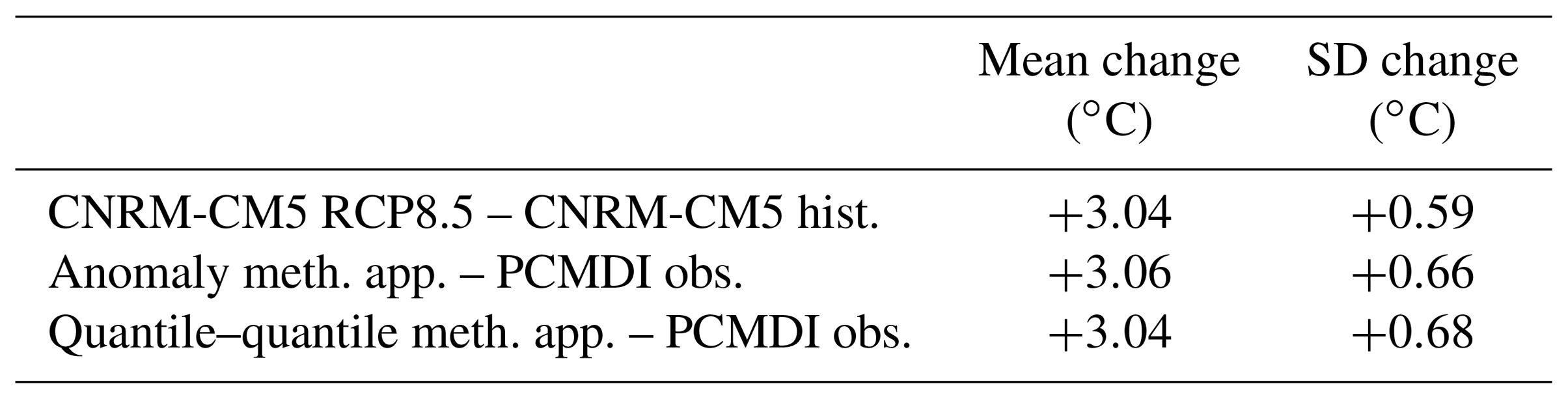
Table 1Mean and standard deviation change between present and future SST data sets for the North Atlantic (45 to 58∘ N, 105 to 85∘ W).
3.1 Sea surface temperatures
3.1.1 Perfect model test
Absolute anomaly or quantile–quantile methods have been used for SST in previous bias-correction applications cited previously in this paper. As a consequence, the utility of a perfect model test here is limited for SSTs, and it was only applied in order to be consistent with the evaluation of the method for SIC. For both methods, the relation between the bias-corrected projected SST and the SST directly obtained from the AOGCM projection is trivial when we replace observed SST with the one from the AOGCM historical simulation, for instance in Eq. (A1). As a result, the resulting errors were null or close to zero, and the results are therefore not presented or discussed.
3.1.2 Real-case application
Here, we present the application of the anomaly and the quantile–quantile methods in a real-case application. For this application, we use SST from the PCMDI observation data set over 1971–2000, from IPSL-CM5A-LR and CNRM-CM5 historical simulation over the same period, and the RCP8.5 scenario over 2071–2100. Histograms of the frequency distribution of SST for different regions of the world (Weddell Sea, central Pacific and North Atlantic) have been plotted in order to compare frequency distributions in the observations, in the GCM historical and future simulations, and in the estimated bias-corrected future SST using the quantile–quantile and anomaly methods (Fig. 4). In this figure, we can appreciate the change in mean and variance between the GCM historical simulation and the GCM future scenario and between the PCMDI observations and the bias-corrected SST scenario. Figure 4c also shows the large cold bias of IPSL-CM5A-LR with respect to the observations in the North Atlantic, as coupled models usually struggle to correctly represent the Atlantic Meridional Overturning Circulation (AMOC). The change in mean and variance due to the climate change signal is more explicitly presented for the North Atlantic for the application with CNRM-CM5 in Table 1. Results from the anomaly method and from the quantile–quantile method are very similar, and both methods succeed in applying the same change in mean and variance coming from the AOGCM scenario to the observations when producing bias-corrected SST.

Figure 4Frequency distribution of SST for PCMDI observations (black), IPSL-CM5A-LR historical (red) over 1971–2000 and RCP8.5 (green), and quantile–quantile method (pink) and anomaly method (blue) applications over 2071–2100 for the Weddell Sea (a), central Pacific (b) and North Atlantic (c).
3.2 Sea-ice concentration
3.2.1 Perfect model test
In this section, we present the results of the application of the perfect model test for the three methods for the bias correction of SIC. The term “perfect model test” is not absolutely pertinent for the evaluation of the look-up table method, as we first computed LUTs using SST and SIC from an AOGCM historical simulation. Then, we used the SST of the climate change projection from the same AOGCM and retrieved SIC with the help of the previously computed LUT. An example of computed LUT using data from the historical simulation of CNRM-CM5 can be seen in the Appendix (Fig. B1). It is noteworthy that this new LUT is significantly different from the one using PCMDI observations (Fig. 1). Even though the use of this LUT for the perfect model test instead of LUTs computed using observed SST and SIC over the AMIP period can be discussed, the use of LUT computed using observations would necessarily produce a poorer result for the reconstruction of SIC of the AOGCM scenario in a perfect model test. Using AOGCM data, inconsistent or missing results were found for most SST bins at or below the freezing point of seawater (−1.8 ∘C). In order to fill the LUT, we therefore fixed SIC =99 % for SST ∘C and linearly interpolated SIC between −1.7 and −2.0 °C.
The perfect model test is more rigorously applied for the evaluation of the relative anomaly and the analogue method, as we simply replaced time series of the observed SIC with the one from the AOGCM historical simulation before applying the method without any specific modification or calibration. For the analogue method, the tested AOGCM projection was excluded from the possible analogue candidates before applying the method and the perfect model test.
Errors (%) after applying the perfect model test are shown for the three methods for the RCP4.5 and RCP8.5 scenarios of the IPSL-CM5A-LR and CNRM-CM5 AOGCM (Fig. 5). These errors are generally lower for the LUT method: the mean root mean square error (RMSE) in the estimation for each scenario for the Arctic and the Antarctic is 4.8 %. The mean error (ME) using this method tends to be positive in the Arctic and negative in the Antarctic seas. Errors using the relative anomaly method exhibit some larger values (mean RMSE =8 %). The errors using the analogue method have intermediate values with respect to the first two methods (mean RMSE =5.9 %). Some of the errors of the analogue method for regions with very complex coastal geography, such as the Canadian Archipelago, are due to the differences in land mask between the tested and the chosen AOGCM as an analogue candidate, despite the care taken for this issue. The pattern of the errors using the iterative relative anomaly seems robust among the different AOGCM scenarios. It is also noteworthy that the pattern of the errors is similar among different methods, especially if we consider the results in the Arctic for the scenarios of the CNRM-CM5 model. The spatial distribution of the errors for HadGEM2-ES SIC in RCP4.5 and RCP8.5 scenarios within the frame of the perfect model test is also presented in the Appendix for the analogue and LUT methods (Fig. B3). The magnitude of the errors is very similar, which increases the confidence in the independence of the results from the selected model.
With the results of the perfect model test, we also performed a comparison between the frequency distribution of the mean SIC in the AOGCM future scenario (here CNRM-CM5, RCP8.5) and in the corresponding estimation using the bias-correction methods (Fig. 6). In these plots, we represented the histogram of the frequency of SIC for four regions: Ross Sea (72–77∘ S, 174∘ E–163∘ W), Weddell Sea (63–73∘ S, 45–25∘ W), Arctic Basin (80–90∘ N, 180∘ W–180∘ E), and the Canadian Archipelago (66–80∘ N, 130–80∘ W). These regions have been chosen because they are the principal regions where a significant amount of sea ice remains by the end of the 21st century under the RCP8.5 scenario. With the LUT method (blue lines in Fig. 6), the distribution of SIC is quite well reproduced in the Arctic (Fig. 6c and d), whereas in the Antarctic seas the distribution (Fig. 6a and b) exhibits well-marked peaks that we do not find in the GCM data set (black lines). The presence of such peaks is easy to explain by taking into account the structure of the LUT as (i) for a given month, the SIC does not always increase monotonically with decreasing SST, and (ii) the discrete nature of LUT is not in favour of a continuous SIC frequency distribution. Moreover, using this method, we find a large underestimation of SIC above 90 %, mainly in the Southern Hemisphere, with almost no occurrence of these high SIC values in the estimations using the LUT method for the Ross and Weddell seas. The frequency distribution of the sea ice using the relative anomaly method (green lines in Fig. 6) is closer to the distribution in the AOGCM, even if there is a slight overestimation of the frequency for concentrations between 70 % and 90 % and an underestimation for very high SICs (above 90 %). Finally, the distribution obtained using the analogue method (red lines in Fig. 6) is very close to the distribution of the original AOGCM scenario. The results are robust because differences in sea-ice frequency distribution between bias-corrected projections and AOGCM scenarios are very similar for other scenarios and coupled models (figures not shown).
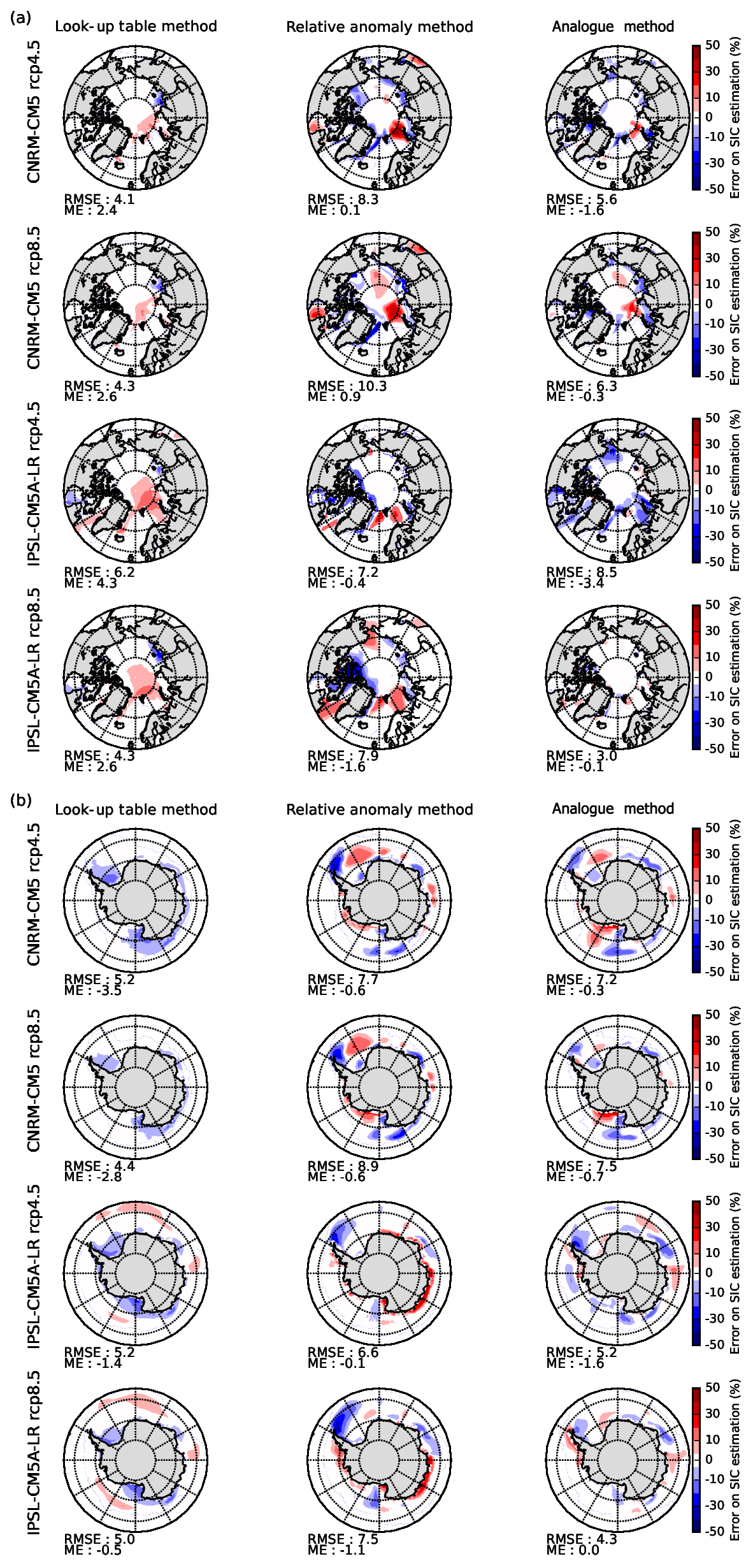
Figure 5Mean error in the estimation of SIC with respect to the original AOGCM future scenario for the LUT, iterative relative anomaly and analogue methods with CNRM-CM5 and IPSL-CM5A-LR RCP4.5 and RCP8.5 scenarios for the Arctic (a) and the Antarctic (b).

Figure 6Frequency distribution of SIC in CNRM-CM5 RCP8.5 scenario (black) and in estimation using different methods in a perfect model test: look-up table (blue), analogue (red) and iterative relative anomaly (green). Regions are (a) Ross Sea (72–77∘ S, 174∘ E–163∘ W); (b) Weddell Sea (63–73∘ S, 43–25∘ W); (c) Arctic Basin (80–90∘ N, 180∘ W–180∘ E); (d) Canadian Archipelago (66–88∘ N, 130–80∘ W).
3.2.2 Real-case application
We applied the three bias-correction methods using PCMDI SIC data from the 1971–2000 period, as well as the IPSL-CM5A-LR and CNRM-CM5 historical data over the same period and data from the RCP4.5 and RCP8.5 scenarios from 2071–2100, in order to obtain future bias-corrected SIC. The reliability of the methods is evaluated by comparing the change in mean and variance between the observations and the bias-corrected projected SICs with the corresponding changes in the original AOGCM scenario with respect to the historical simulation. We consider here that an ideal method should apply the same statistical changes to observed sea ice as the one present in the climate change projection used to derive climate change signal.
In Fig. 7, the bias-corrected mean SIC change is plotted against the corresponding change in mean SIC in the AOGCM scenario used to determine the climate change signal. All points in the plot are obtained by the same four AOGCM scenarios as well as the same four “test regions” as in the previous section (Ross and Weddell seas, Arctic Basin, Canadian Archipelago). Similarly, in Fig. 9, applied changes in standard deviation for the bias-corrected projected SIC are plotted against the corresponding standard deviation change in the AOGCM climate change experiment.
For the LUT method (Fig. 7a), future SSTs have been bias corrected using the quantile–quantile method before using computed LUT for the retrieval of future SIC. Using this method, there seems to be no systematic error in the applied change in mean SIC. The mean error in the estimation of the change in mean SIC for every region and scenario is −2.2 % and the RMSE is 42 %. The spread of the points seems to increase for stronger decreases in sea ice. Main outliers with a high overestimation of the decrease in SIC are points representing the evolution of sea ice in the Weddell Sea, mainly for CNRM-CM5 scenarios. If we consider change in SIC variability (Fig. 9a), systematic error (−14.9 %) and RMSE (69.3 %) are strong. The decrease in SIC variability in the Antarctic seas in the projection is strongly overestimated. Indeed, due to the structure of the LUTs themselves, the variability of SIC in the bias-corrected projections is much lower than in the observations or in the original scenarios.
The application of the relative anomaly method shows a more general overestimation (ME %; RMSE =52.2 %) of the decrease in mean SIC (Fig. 7b). This overestimation is more pronounced for the Weddell Sea area and for the scenarios of the CNRM-CM5 model. Only the decrease in mean SIC in the Arctic Basin is correctly reproduced with respect to the AOGCM scenarios. Concerning the change in SIC variability (Fig. 8b), the scores are comparable to the application of the LUT method (ME %; RMSE =64.7 %). The increase in variability in the Arctic Basin and in the Canadian Archipelago is correctly reproduced, whereas for the Antarctic seas and particularly the Weddell sector, the decrease in SIC variability is once again dramatically overestimated.
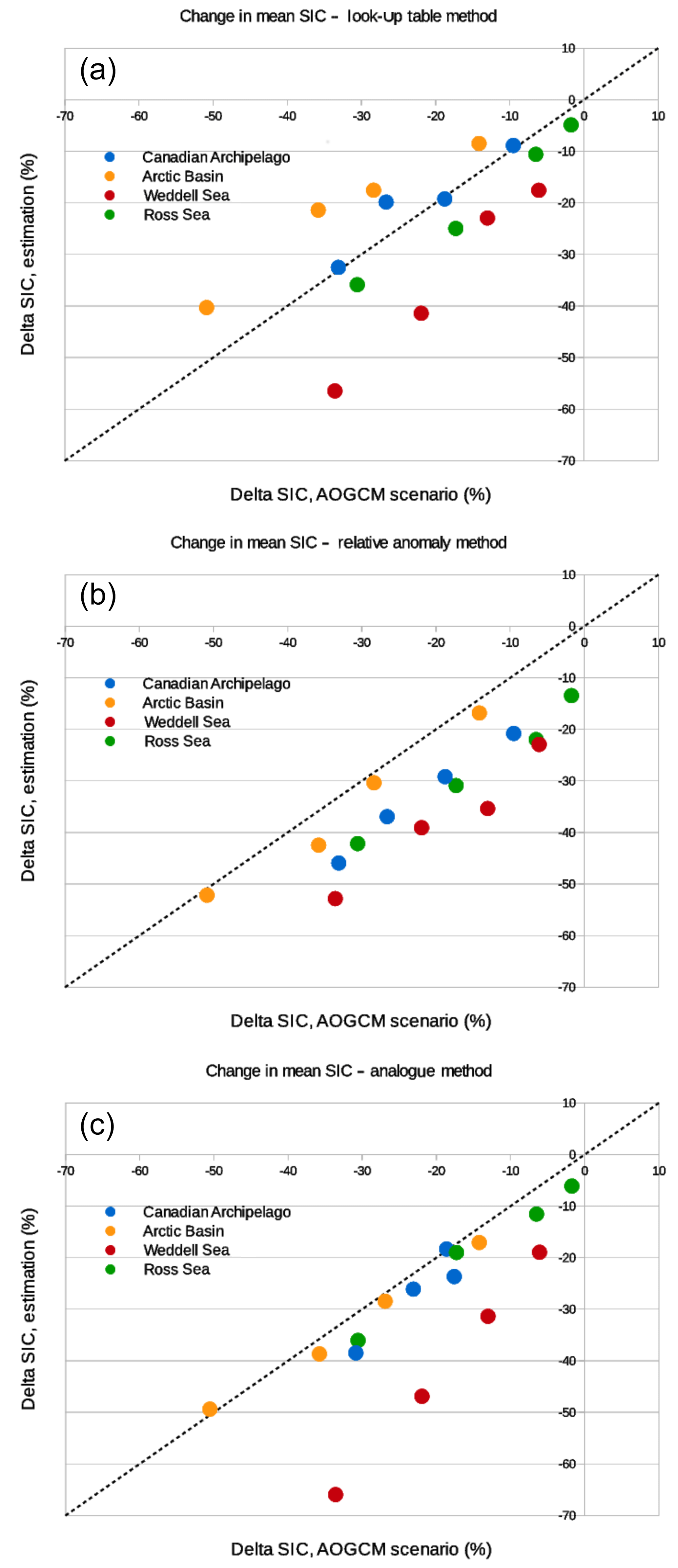
Figure 7Change in mean bias-corrected SIC projections using (a) look-up table, (b) iterative relative anomaly and (c) analogue methods against corresponding mean change in the A OGCM projection for the four test regions: Canadian Archipelago (blue), Arctic Basin (orange), Weddell Sea (red) and Ross Sea (green) for projections from CNRM-CM5 and IPSL-CM5A-LR.

Figure 8Change in bias-corrected SIC projection standard deviation using (a) look-up table, (b) iterative relative anomaly and (c) analogue methods against corresponding mean change in the AOGCM projection for the four test regions: Canadian Archipelago (blue), Arctic Basin (orange), Weddell Sea (red) and Ross Sea (green) for projections from CNRM-CM5 and IPSL-CM5A-LR.

Figure 9Mean error in the estimation of SST with respect to the corresponding original AOGCM scenario after applying the analogue method for sea ice, the quantile–quantile method for SST, and the correction for SST and SIC consistency for the Arctic (a) and the southern oceans (b).
Finally, the application of the analogue method gives intermediate scores (ME %; RMSE =48.7 %) with respect to the two previous methods for the estimation of the change in mean SIC (Fig. 7c). These scores are greatly deteriorated by distinct outliers corresponding to the Weddell Sea sector for each AOGCM scenario, with an overestimation of the decrease in sea ice. As for the relative anomaly method, the change in SIC variability (Fig. 8c) is correctly reproduced (ME %; RMSE =60.3 %), especially in the Arctic, while there is an overestimation of the decrease in variability around Antarctica, particularly for the Weddell Sea.
3.3 Consistency between sea surface temperature and sea-ice concentration
As bias corrections of SST and sea ice are performed separately, the physical consistency between the two variables needs to be ensured a posteriori. To do so, three different issues are examined.
-
There is a considerable amount of sea ice (>15 %) in the corrected scenario in which the SST is above the freshwater freezing point (273.15 K). In this case, we set SST equal to the seawater freezing point (271.35 K) for any SIC equal to or greater than 50%. If the future calculated SIC is between 15 % and 50 %, the future SST is obtained by linearly interpolating between the seawater freezing point and the freshwater freezing point.
-
The future corrected SST is below the freshwater freezing point but there is no significant (<15 %) SIC in the bias-corrected scenario. In this case, we put the SST of the concerned grid point equal to the freshwater freezing point.
-
SST has been used to remove very localised suspicious sea ice (no ice) in the Arctic in summer. Any sea ice for SST above 276.15 K has been removed, this temperature being the highest temperature at which a significant amount of sea ice (15 %) is found in the Arctic for the computed LUT using PCMDI data.
The impact of these modifications has been evaluated using the framework of the perfect model test. After applying the analogue method for SIC and the quantile–quantile method for SST in a perfect model approach, we applied the correction for SST and SIC consistency and compared obtained SSTs to the original AOCGM future scenario used to carry out the experiment. The error can be seen in Fig. 9 for the application of the method with IPSL-CM5A-LR and CNRM-CM5 scenarios. Error is negligible in most regions. Very locally, it can reach up to 1 ∘C. These regions generally correspond to regions where the analogue method has shown some errors for the reconstruction of sea ice, especially for CNRM-CM5 scenarios. The occurrences of the three cases mentioned above have been assessed for both the perfect method test and the real-case application. The first and third cases are very rare and about 1 % or less of global oceanic surfaces experience at least one case during a 30-year experiment. The second case is more frequent; more than 20 % of global oceanic surfaces experience at least one occurrence during a 30-year experiment, while the mean occurrence at each time step is about 1 % to 2 % of global oceanic surfaces. This case is responsible for the small (0.25 to 0.5 K) but widespread warm bias in SST that can be seen in the Antarctic seas for the reconstruction of IPSL model scenarios in Fig. 9. Nevertheless, this slight decrease in the quality of the reconstruction of SST is worth considering in order to ensure physical consistency between SST and SIC.
3.4 Sea-ice thickness
The original formulation by Krinner et al. (1997) was parameterised for both hemispheres. We will therefore first present results for the original unique parameter set applied to both hemispheres. In a second step, we will present results for separate Arctic and Antarctic parameter sets, yielding a better fit to the observations. The reasoning is that, at the expense of generality of the diagnostic parameterisation, one could argue that the strong difference between the Arctic and Antarctic geographic configuration – a closed small ocean favouring ice ridging and thus thicker sea ice in the Arctic versus a large open ocean favouring thinner sea ice around Antarctica – justifies choosing different parameter sets for the two hemispheres. As changes in the position of the continents will be irrelevant over the timescales of interest here, climate change experiments will not be adversely affected by this loss of generality.
3.4.1 Option 1: global parameter set
A comparison between the observed (Lindsay and Schweiger, 2015) and our diagnosed evolution of the Arctic mean SIT is given in Fig. 10a. The geographical patterns of the observed (in fact, observation-regressed) and parameterised Arctic ice thickness for March and September over the observation period 2000–2013 (Fig. 11a) do bear some resemblance, but they also show some clear deficiencies in the diagnostic parameterisation. The diagnostic parameterisation reproduces high SIT north of Greenland and the Canadian Archipelago linked to persistent strong ice cover, but underestimates maximum ice thickness (due in part to compression caused by the ocean surface current configuration). Thinner sea-ice over the seasonally ice-free parts of the basin is reproduced, but it is actually too thin, particularly in winter (for example in the Chukchi Sea). Obvious artifacts appear in September north of about 82∘ N where the SIC in the ERA-Interim data set clearly bears signs of limitations due to the absence of satellite data.
Both for spring (October–November) and fall (May–June), our diagnosed SIT (Fig. 12) compares generally well with the ICESat data except for an overestimate in the Weddell Sea in both seasons. The geographical pattern of alternating regions with thin and thick sea ice is remarkably well reproduced.
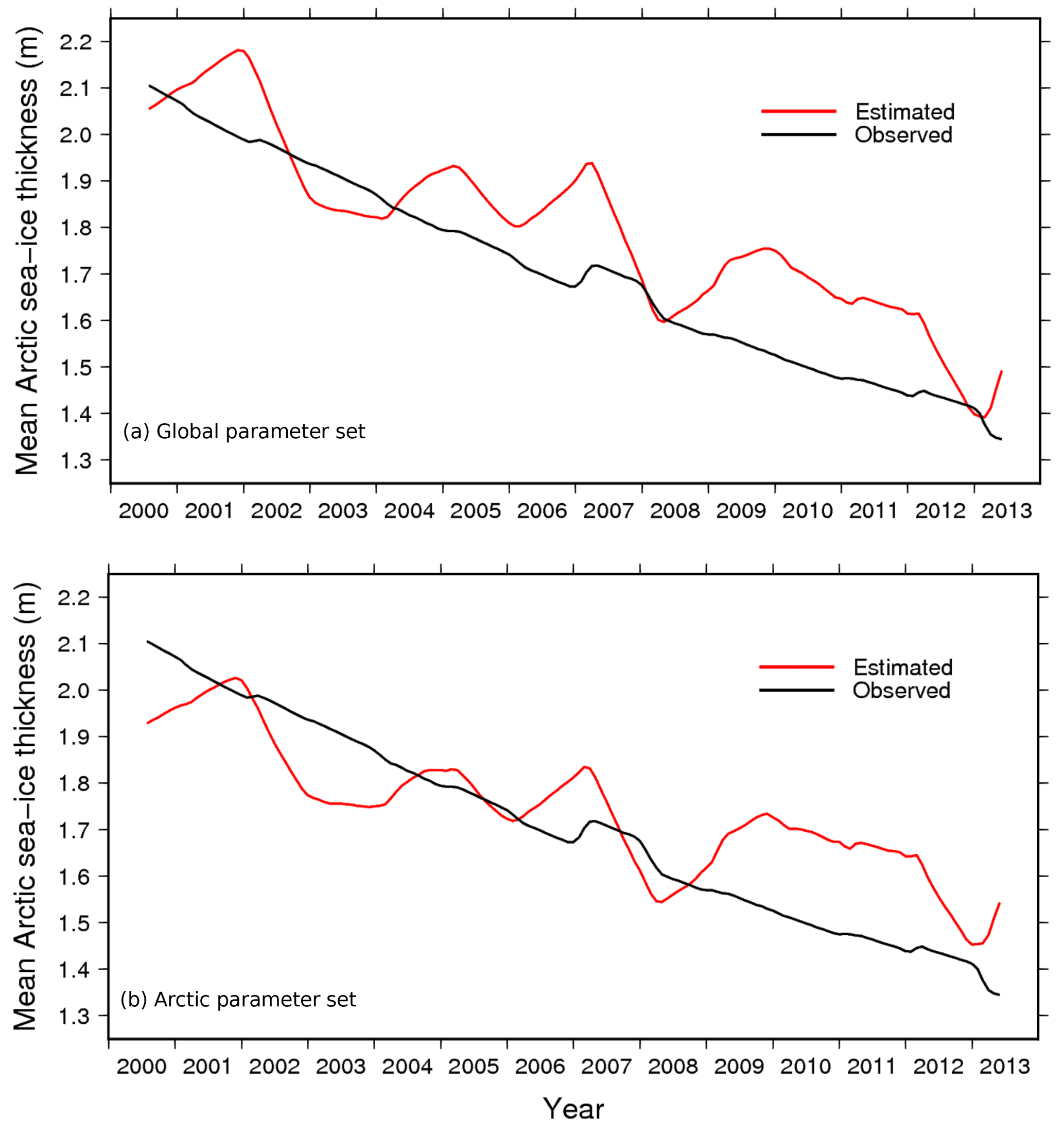
Figure 10Observed (black, after Lindsay and Schweiger, 2015) and diagnosed (red) 12-month moving average mean sea-ice SIT of the Arctic basin (see Fig. 11) using (a) the global parameter set and (b) the Arctic-specific parameter set. Slight differences to Figure 12 of Lindsay and Schweiger (2015) appear because here we mask ice-free (SIC <15 %) areas that have a finite, non-zero ice thickness in the regression proposed by Lindsay and Schweiger (2015), who extend their regression to the entire Arctic Basin in all seasons.
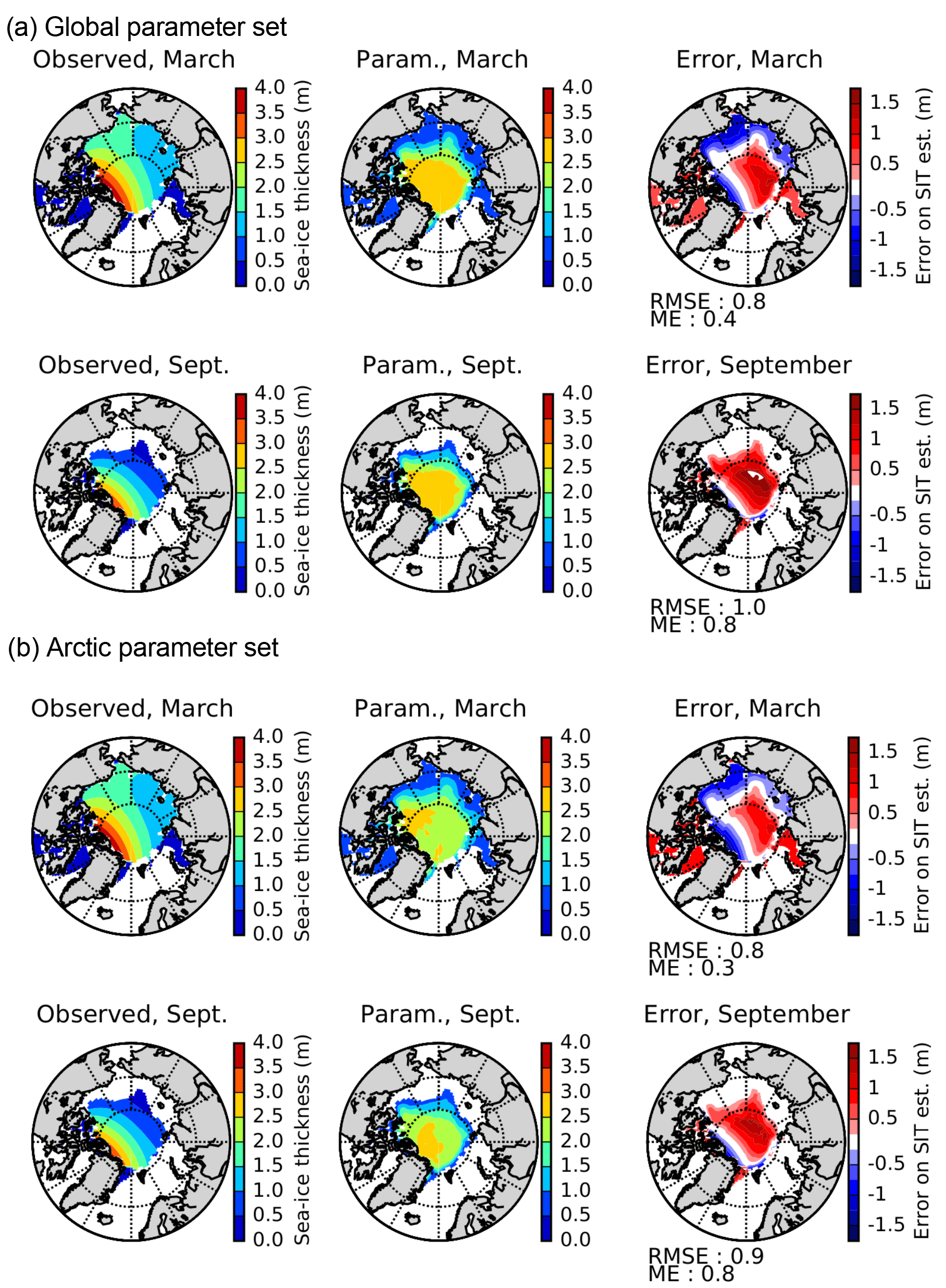
Figure 11Observed (regressed, Lindsay and Schweiger, 2015) and parameterised Arctic SIT (in m) for March and September and the difference between these (right) with (a) the global parameter set and (b) the Arctic parameter set.
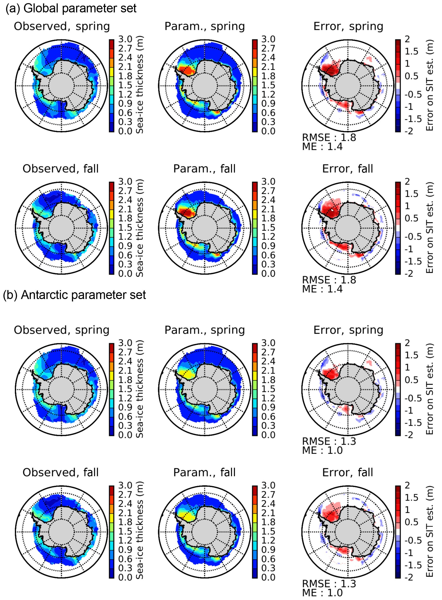
Figure 12Observed Kurtz and Markus (2012) and parameterised Antarctic sea-ice thickness (in m) for spring and fall and the difference between these (right) with (a) the global parameter set and (b) the Antarctic-specific parameter set.
3.4.2 Option 2: separate Arctic and Antarctic parameter sets
A slightly better fit for the two poles can be obtained with separate parameter sets. For the Arctic, it seems desirable to increase winter SIT in the Chukchi Sea area (by increasing c3 slightly) and to decrease the average SIT over the central Arctic (by decreasing c2). Figures 10b and 11b show results for the Arctic with c1=0.2 m, c2=2.4 m and c3=3 m. The spatial fit is slightly better, but the recent Arctic mean decadal trend towards decreased average SIT is somewhat less well reproduced. For the Antarctic, the main feature to improve is the maximum ice thickness in the Weddell Sea, which can be decreased by lowering c2 to 2.0 m. The Antarctic parameter set then becomes c1=0.2 m, c2=2 m and c3=2 m. The result (Fig. 12b) is indeed a decreased thickness of the perennial Weddell Sea ice with little impact elsewhere.
In any case, these hemisphere-specific sea-ice parameter sets are not very different from each other and are fairly similar to the original formulation.
4.1 Sea surface temperatures
The bias correction of projected SST coming from AOGCM scenarios is fairly easy to deal with, and different appropriate solutions have already been proposed in the literature (Ashfaq et al., 2011; Hernández-Díaz et al., 2017; Holland et al., 2010; Krinner et al., 2008). In these papers, it has been demonstrated that the use of bias-corrected SSTs has considerable influences on the modelled climate and its response in projected scenarios for regions and processes as different as precipitation and temperature in the tropics, the West African monsoon and the climate of Antarctica.
In this paper, we reviewed two existing bias-correction methods and propose a validation that allows for an objective evaluation of the efficiency of these methods with the use of a perfect model test and a real-case application. Since both methods show no biases in the perfect model test and succeed in reproducing the change in mean and variability coming from the AOGCM future scenarios, we can be confident in the use of these methods for the bias correction of future AOGCM scenarios.
4.2 Sea-ice concentration
SIC is a quantity that has to remain strictly bounded between 0 % and 100 %, exhibits some sharp gradients, and has to remain physically consistent with SST. Therefore the empirical bias correction of future SIC from coupled model scenarios is a much more complex issue to deal with than the bias correction of SSTs. The absence of satisfying solution proposals for this issue in the literature has led to the incorrect bias correction of future SIC in a recent study (Hernández-Díaz et al., 2017). Yet, the proposal of convenient solutions for the bias correction of sea ice for projected scenarios is crucial for the community interested in the downscaling of climate scenario experiments for polar regions.
The perfect model test revealed that the LUT method shows some reduced errors over most regions (Fig. 5). However, we have seen that the frequency distribution of future SIC obtained using this method is very different than the original distribution in the AOGCM and unavoidably exhibits some peaks due to the structure of LUT (Fig. 6). Moreover, the absence of SIC above 90 % in the Antarctic is also a considerable limitation to the method considering the large differences in terms of heat and moisture exchanges in winter between an ocean fully covered by sea ice and an ocean that exhibits some ice-free channels (Krinner et al., 2010). In addition, the use of SST as a proxy for SIC is physically questionable, as we should expect a large SIC gradient around the freezing point. The fact that both SST and SIC are averaged over a long period (1 month) and over a considerable area () is probably the main reason why we nevertheless find a relation between the two variables. The real-case application of the method also shows some difficulties for the reconstruction of large decreases in mean SIC (Fig. 7a) as well as a poor reconstruction of the change in variability in future SIC (Fig. 8a).
The relative anomaly method (Krinner et al., 2008) shows the largest spatial mean errors in the perfect model test (Fig. 5). The structure of some errors seems to be constant across the reconstruction of different climate scenarios used in the perfect model test. The empirical reduction of SIC by an iterative “erosion” from the edges of sea-ice-covered regions most likely has the tendency to overestimate the decrease in sea ice for some coastal regions, while it probably fails to reproduce some processes involved in the disappearance of sea ice in the future, such as the inflow of warmer waters through the Barents Sea or the Bering Strait in the Arctic. The real-case application of the relative anomaly method has shown some systematic negative errors in the reconstruction of the decrease in mean SIC (Fig. 7b) and a substantial overestimation of the decrease in variability in the Antarctic seas (Fig. 8b).
The evaluation of the analogue method with the perfect model test shows that the mean error can be locally slightly higher than for the LUT method (Fig. 5). However, the frequency distribution of the bias-corrected SIC perfectly reproduces the frequency distribution of the sea ice in the original AOGCM scenario (Fig. 6). The real-case application of the method succeeds in reproducing the change in mean and variability of SIC for most of the tested regions and scenarios (Fig. 7c). However, the decrease in mean (Fig. 7c) and variability (Fig. 8c) of the sea ice in the Antarctic, particularly the Weddell Sea, is also largely overestimated using this method. With respect to the relative anomaly method, the fact that we use observed or AOGCM-simulated sea-ice maps to reconstruct estimated future sea ice, and that we use a criterion for both SIA and SIE, allows us to better reproduce some critical features of future sea-ice cover and to obtain a more realistic frequency distribution. It should be noted that in the perfect model test as well as in the real-case application, the original AOGCM is not present among the possible analogue candidates. If this is done, the results are even better using this method.
The fact that the analogue method and the relative anomaly method share the same errors in the real-case application with a strong overestimation of the decrease in mean and variability of the sea ice in the Weddell Sea, particularly for the scenarios of the CNRM-CM5 model, is not a coincidence. For both methods, the targeted future SIE (or SIA) for a given sector is a product of the division of the integrated SIE (SIA) in the AOGCM scenario by the corresponding quantity in the historical simulation. As a consequence, the targeted projected SIE (SIA) for a given sector and a given month is null when the integrated SIE (SIA) is null in the future AOGCM scenario. Therefore, the bias in the scenario is not corrected in that case. The fact that both methods overestimate the decrease in sea ice mainly for CNRM-CM5 scenarios is linked to the fact that the historical simulation of this AOGCM shows some considerable negative biases for the sea ice in the Weddell Sea with respect to the observations. Consequently, SIC in the Weddell Sea in the CNRM-CM5 RCP8.5 scenario is low and the number of months with a complete disappearance of sea ice is large. For these months, SIC in these sectors is not bias corrected with the latter two methods. This means that although the methods described here are in principle applicable to any AOGCM output, it seems wise to exclude AOGCMs with a large negative bias in sea ice from their historical simulation as initial material for the bias correction.
4.3 Sea-ice thickness
Given the simplicity of the proposed diagnostic SIT parameterisation, the results are, at least in some aspects such as the predicted average Arctic sea-ice thinning, surprisingly good. The central Arctic SIT results are clearly adversely affected by the input SICs north of 82∘ N. Arctic winter SIT in the marginal seas appears underestimated. In the Antarctic, the spatial pattern of SIT is very well represented.
We think that in the absence of pan-Arctic and pan-Antarctic satellite-based data before approximately 2000, this parameterisation can serve as a surrogate and that it can, because it seems to have predictive power, also serve for climate change experiments with AGCMs or RCMs. Because of its simplicity, implementing this parameterisation should not be too complicated in any case provided the model does explicitly take into account SIT in its computations of heat flow through sea ice. In that case, SIT can either be calculated online (with the need to keep track of annual minimum SIC during the execution of the code) or be input as a daily boundary condition along with the SIC.
Of course, another possibility would be to prescribe SIT anomalies from coupled models. In this case, it would probably be wise to compute the prescribe SIT using its relative thickness changes. For example, in a climate change experiment, this would read . Problems could of course occur in areas where the coupled model simulates no sea-ice cover at present. A physically consistent diagnostic parameterisation of SIT as a function of constructed SIC, as proposed here, would not suffer from such problems.
In any case, it is very probable that Arctic SIT will further decrease as multi-year sea ice will be replaced by a predominantly seasonal sea-ice cover. This should probably be taken into account in future modelling exercises similar to CORDEX or HighResMIP given the non-negligible impact of sea-ice thinning on winter heat fluxes in particular.
4.4 General considerations on bias correction of oceanic forcings
As already mentioned, one may doubt whether it is possible to bias correct a GCM that has overly large biases in present-day climate. Indeed, most of the bias-correction methods rely on the hypothesis than the climate change signal coming from an AOGCM scenario is not dependent on the bias in the historical simulations. This hypothesis can largely be questioned in a non-linear system (formed by SIC and SST). For example, in a model with a large negative bias in sea ice for present-day climate, most of the additional energy due to an enhanced greenhouse effect will be used to heat the ocean, while it would be primarily used to melt sea ice in a model with a correct initial sea-ice state. For such a model, the reliability of the climate change signal in SST is thus necessarily questionable. The selection of climate models based on their credibility for climate change scenarios is a complex issue (Baumberger et al., 2017; Brekke et al., 2008) dependent on the purposes, processes and region of study. Whether the climate change signal should be corrected remains on open question (Ehret et al., 2012), even though there are good reasons to believe that model biases are time invariant (Maurer et al., 2013).
The skills of coupled GCMs in reproducing the observed climate and its variability for a region of interest are often evaluated in order to use the GCM output as forcing for downscaling experiments. However, the skills of atmospheric GCMs are generally better when forced by observed oceanic boundary conditions (Ashfaq et al., 2011; Hernández-Díaz et al., 2017; Krinner et al., 2008; Li and Xie, 2014). Similarly, even though bias-correction methods have some limitations, for future climate experiments, there are good reasons to believe that simulations produced using bias-corrected oceanic forcings bear reduced uncertainties with respect to simulations realised with “raw” oceanic forcings from coupled model scenarios such as those from the CMIP5 experiments.
Bias-corrected oceanic forcings can be used to force a regional climate model (RCM), but in this case an additional modelling step has to be carried out, as bias-corrected oceanic forcings should be used to force an atmosphere-only GCM that will provide atmospheric lateral boundary conditions for the RCM in order to ensure consistency between oceanic and atmospheric forcings, such as in Hernández-Díaz et al. (2017). In this framework, the use of a variable-resolution GCM which allows us to directly use bias-corrected oceanic forcings and downscale climate scenarios is an alternative worth considering, as it also allows for two-way interactions between the downscaled regions and the general atmospheric circulation.
In this paper, we reviewed existing methods for the bias correction of SST and SIC and proposed new ones, such as the analogue method for sea ice. We also proposed validation methods that allow for an objective evaluation of bias-correction methods with the use of a perfect model test and real-case applications.
The bias correction of SST is an issue that has already been widely addressed in recent papers and its importance for the modelling and downscaling of future climate scenarios has been demonstrated for multiple regions of the world. In our analysis, we were able to demonstrate the reliability and the suitability of absolute anomaly and quantile–quantile methods for the bias correction of future SST scenarios.
The bias correction of SIC is a more difficult issue to address. With the analogue method, we propose a method that shows promising results in most cases and that allows for a reconstruction of future SIC with a realistic frequency distribution. However, the fact that the relative anomaly between an AOGCM scenario and its historical simulation is also used in this method in order to determine future targeted sea-ice extent and area prevents the bias correction of cases in which sea ice disappears entirely in a given sector or even a hemisphere. Despite the absence of a perfect and definite solution to this issue, we propose a new and improved method as well as a convenient, objective way to evaluate bias-correction methods for climate scenarios. The bias correction of sea ice is currently somewhat overlooked by the community. The application of a multivariate bias-correction method (Cannon, 2016) is also a perspective that could help with the bias correction of SST and SIC projected scenarios at the same time. Nevertheless, corrected SIC using the analogue method represents a substantial improvement with respect to other previously existing bias-correction methods for sea-ice scenarios and will therefore be made available to anyone willing to use them as forcing for bias-corrected downscaling experiments.
The FORTRAN code enabling the generation of bias-corrected future SST and SIC using CMIP5 scenarios and PCMDI data as input is publicly available for each method via https transfer (https://mycore.core-cloud.net/index.php/s/80x0Te7CQ0BowNG, last access: 9 January 2019) or using the following DOI: https://doi.org/10.17605/OSF.IO/EFUY2 (Beaumet and Krinner, 2018a). Bias-corrected future CMIP5 scenarios (RCP4.5 and 8.5) realised within the framework of this study (IPSL-CM5A-LR and CNRM-CM5) are available as well (https://mycore.core-cloud.net/index.php/s/Q1cIsS71Mo4vGrG, last access: 9 January 2019) or by using the DOI https://doi.org/10.17605/OSF.IO/GMH8C (Beaumet and Krinner, 2018b).
A1 Anomaly method
This frequently used method (Krinner et al., 2008) simply consists of adding the SST anomaly coming from the difference between a coupled AOGCM projection and the corresponding historical simulation to the present-day observations. In practice, for each grid point, the difference between the SST for a given month in the future from a climate change simulation and the climatological mean SST in the corresponding historical simulation from the same coupled AOGCM is added to the observed climatological mean SST (e.g. PCMDI, 1971–2000).
In Eq. (A1), SSTFut, est is the estimated future SST for a given month, the observed climatological monthly mean, SSTFut, AOGCM the model future SST for a given month in the future AOGCM scenario and the model climatological monthly mean in the AOGCM historical simulation for the same reference period as for the observed climatology. As a result, the reconstructed SST time series has the chronology of the AOGCM projected scenario.

Figure A1Illustration of the quantile–quantile method for min. and max. of SST time series for a grid point in the central Pacific: GCM historical simulation (blue, a), GCM projected scenario (red, a), observed SST (dashed, b), reconstructed future SST (thick, b).
A2 Quantile–quantile method
This method has been proposed and described in Ashfaq et al. (2011). It consists of adding, for each grid point and each calendar month's quantile in the observations, the corresponding quantile change in the GCM data set, i.e. the difference between the maximum SST in the projected scenario and in the historical simulation, between the second highest SSTs in the two simulations and so on for each ranked SST quantile. However, unlike Ashfaq et al. (2011), we did not create a new SST field for the present by replacing SST from the GCM in the historical period with its corresponding quantile in the observations, but we directly added the quantile change to the corresponding quantile of the observational time series (Fig. A1). This conserves the chronology of the observations and their inter-annual variability in estimated SSTs for the future. In our results, we noticed a large fine-scale spatial variability in the constructed bias-corrected SSTs that was due to the large spatial variability of the climate change increments (quantile change) calculated individually for each pixel. To fix this, we applied a slight spatial filtering (three-grid-point Hann box filter; Blackman and Tukey, 1959) of the quantile shifts in order to produce more consistent SST fields.
B1 LUT method
This section presents the LUT linking SST and SIC using data from the CNRM-CM5 historical simulation (Fig. B1). The LUT obtained is clearly different from the one obtained using SST and SIC from the observations (Fig. 1).
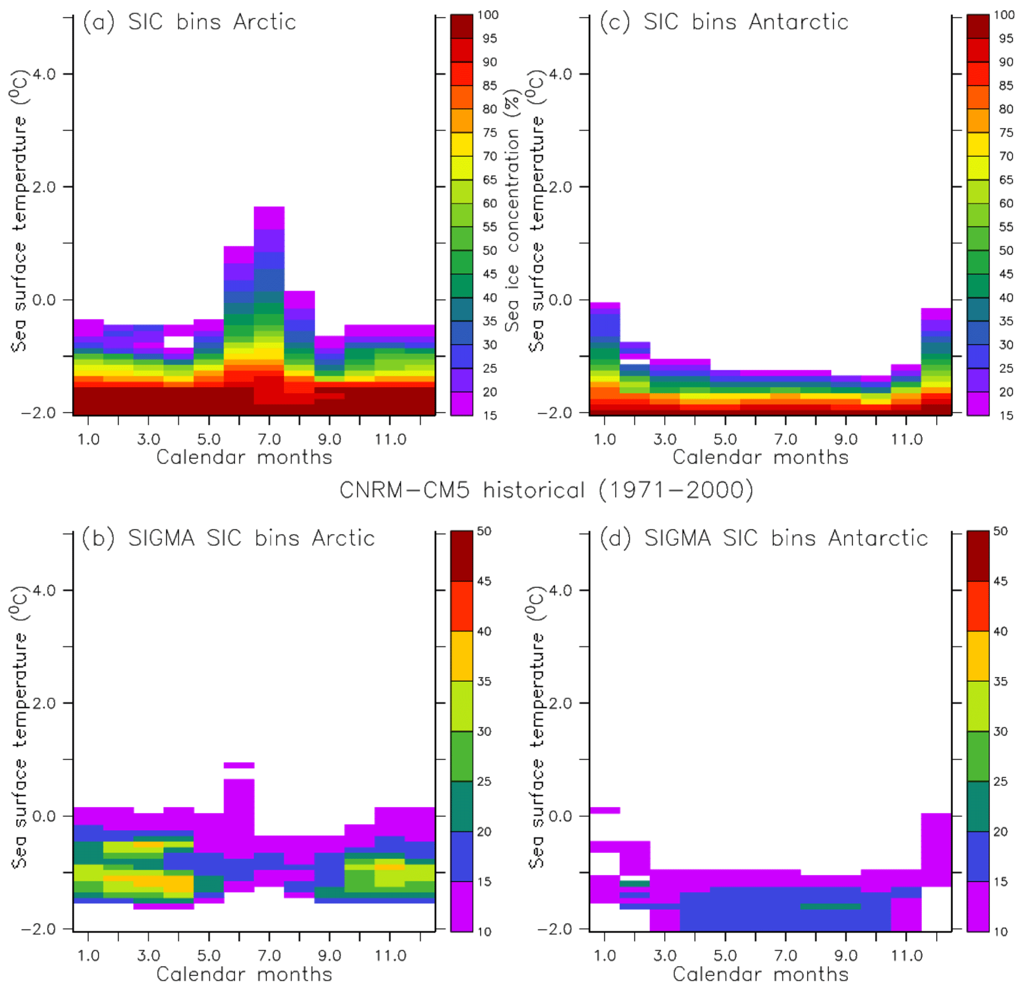
Figure B1Look-up tables linking SST and SIC for the Arctic (a) and the Antarctic (c) built using 1971–2000 CNRM-CM5 historical simulation data and the associated uncertainty (root mean square error) in the computed SIC average (b, d).
Table B1CMIP5 AOGCMs used to build the analogue candidate list.
B2 Analogue method
In this section, the sectors of the Arctic and the Antarctic used in the analogue method for the bias correction of SIC are presented (Fig. B2). We also present the list of AOGCMs used to build the analogue candidate library.
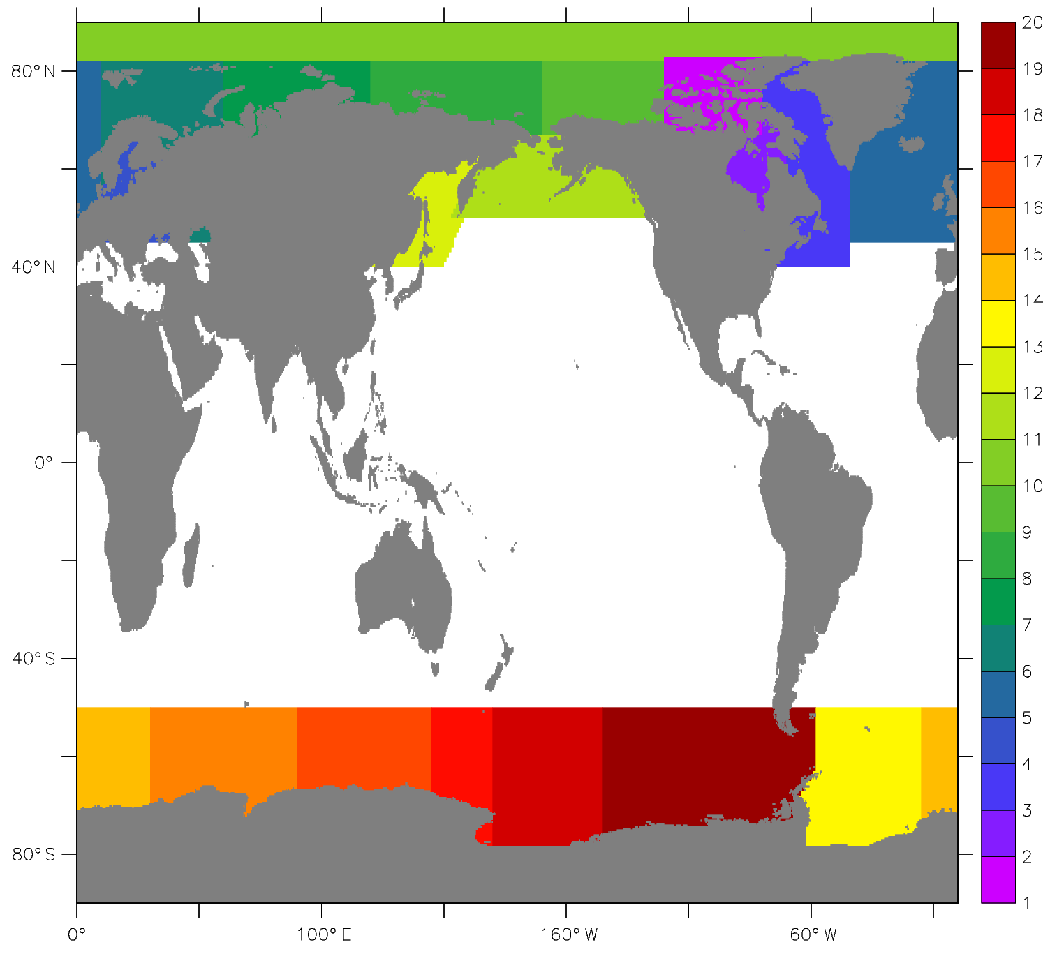
Figure B2Geographical sectors used for the analogue method: (1) Canadian Archipelago, (2) Hudson Bay, (3) Baffin Bay and the Danish straits, (4) north-east Atlantic, (5) Baltic Sea, (6) Barents Sea, (7) Kara and White Sea, (8) Laptev and East Siberian Sea, (9) Beaufort Sea, (10) Arctic Basin, (11) Bering Sea, (12) Sea of Okhotsk, (13) Weddell Sea, (14) East Atlantic, (15) West Indian Ocean, (16) East Indian Ocean, (17) West Pacific, (18) Ross Sea, (19) Amundsen and Bellingshausen Sea.
B3 Results of the perfect model test
In this section, supplementary results are presented for the application of the look-up table method and the analogue method for the reconstruction of SIC in HadGEM2-ES RCP4.5 and RCP8.5 scenarios within the framework of the perfect model test. The spatial distribution of the errors (%) is presented in Fig. B3. The magnitude of the errors is very similar to those presented for CNRM-CM5 and IPSL-CM5-LR in the main part of the article (Fig. 5). Both methods are successful in reconstructing the model SIC fields in most part of the Arctic and the Southern Ocean. Here again, the analogue method has some biases in the Canadian Archipelago region due to differences in land masks between the bias-corrected AOGCM and the selected analogue candidate from the library.

Figure B3Mean error in the estimation of SIC with respect to the original AOGCM future scenario within the framework of the perfect model test for the LUT and the analogue methods with HadGEM2-ES RCP4.5 and RCP8.5 scenarios for the Arctic (a) and the Antarctic (b).
JB wrote most of the paper, participated in the development of the analogue, the look-up table and the iterative relative anomaly methods for sea ice, and carried out the perfect model tests and “real-case” applications. GK participated in the development of the analogue, the look-up table and the relative anomaly methods for sea ice and wrote the sea-ice thickness section of the paper. RH provided material and advice for the application of the look-up table method. LL deserves credit for the original idea and the first developments of the analogue method. All authors actively contributed to the reviewing process aiming at the improvement of the paper.
The authors declare that they have no conflict of interest.
This study was funded by the Agence Nationale de la Recherche through
contracts ANR-14-CE01-0001-01 (ASUMA) and ANR-15-CE01-0003 (APRES3). We
acknowledge the World Climate Research Programme's Working Group on Coupled
Modelling, which is responsible for CMIP, and we thank the climate modelling
groups participating in CMIP5 for producing and making available their model
output. For CMIP the U.S. Department of Energy's Program for Climate Model
Diagnosis and Intercomparison provides coordinating support and led
the development of software infrastructure in partnership with the Global
Organization for Earth System Science Portals. Rein Haarsma was funded
through the PRIMAVERA project under grant agreement 641727 in the European
Commission's Horizon 2020 research programme. We thank Florian Gallo and two
anonymous referees for constructive comments aiming to improve the
quality of this paper.
Edited by: Olivier Marti
Reviewed by: Florian Gallo and two anonymous referees
Agosta, C., Favier, V., Krinner, G., Gallée, H., Fettweis, X., and Genthon, C.: High-resolution modelling of the Antarctic surface mass balance, application for the twentieth, twenty first and twenty second centuries, Clim. Dynam., 41, 3247–3260, https://doi.org/10.1007/s00382-013-1903-9, 2013. a, b
Ashfaq, M., Skinner, C. B., and Diffenbaugh, N. S.: Influence of SST biases on future climate change projections, Clim. Dynam., 36, 1303–1319, https://doi.org/10.1007/s00382-010-0875-2, 2011. a, b, c, d, e, f
Baumberger, C., Knutti, R., and Hirsch Hadorn, G.: Building confidence in climate model projections: an analysis of inferences from fit, WIREs Clim. Change, 8, e454, https://doi.org/10.1002/wcc.454, 2017. a
Beaumet, J. and Krinner, G.: SSC Bias correction – Source code, OSF, https://doi.org/10.17605/OSF.IO/EFUY2, 2018a. a
Beaumet, J. and Krinner, G.: SSC Bias correction – Data, OSF, https://doi.org/10.17605/OSF.IO/GMH8C, 2018a. a
Blackman, R. and Tukey, J. W. (Eds.): Particular pairs of windows, in: The measurement of power spectra, from the point of view of communications engineering, Dover Publications, inc., New York, chap. B5, 95–100, 1959. a
Brekke, L. D., Dettinger, M. D., Maurer, E. P., and Anderson, M.: Significance of model credibility in estimating climate projection distributions for regional hydroclimatological risk assessments, Climatic Change, 89, 371–394, https://doi.org/10.1007/s10584-007-9388-3, 2008. a
Cannon, A. J.: Multivariate bias correction of climate model output: Matching marginal distributions and intervariable dependence structure, J. Climate, 29, 7045–7064, 2016. a
Church, J. A., Clark, P. U., Cazenave, A., et al.: Sea level change, in: Climate change 2013: the Physical Science Basis. Contribution of Working Group I to the Fifth Assessment Report of the Intergovernmental Panel on Climate Change, edited by: Stocker, T. F., Qin, D., Plattner, G.-K., Tignor, M. M. B., Allen, S. K., Boschung, J., Nauels, A., Xia, Y., Bex, V., and Midgley, P. M., Cambridge University Press, Cambridge, United Kingdom and New York, NY, USA, chap. 13, 1137–1216, 2013. a
de Elía, R., Laprise, R., and Denis, B.: Forecasting Skill Limits of Nested, Limited-Area Models: A Perfect-Model Approach, Mon. Weather Rev., 130, 2006–2023, https://doi.org/10.1175/1520-0493(2002)130<2006:FSLONL>2.0.CO;2, 2006. a
Denis, B., Laprise, R., Caya, D., and Côté, J.: Downscaling ability of one-way nested regional climate models: the Big-Brother Experiment, Clim. Dynam., 18, 627–646, https://doi.org/10.1007/s00382-001-0201-0, 2002. a
Ehret, U., Zehe, E., Wulfmeyer, V., Warrach-Sagi, K., and Liebert, J.: HESS Opinions “Should we apply bias correction to global and regional climate model data?”, Hydrol. Earth Syst. Sci., 16, 3391–3404, https://doi.org/10.5194/hess-16-3391-2012, 2012. a
Flato, G., Marotzke, J., Abiodun, B., et al.: Evaluation of Climate Models, in: Climate Change 2013: The Physical Science Basis. Contribution of Working Group I to the Fifth Assessment Report of the Intergovernmental Panel on Climate Change, edited by: Stocker, T. F., Qin, D., Plattner, G.-K., Tignor, M. M. B., Allen, S. K., Boschung, J., Nauels, A., Xia, Y., Bex, V., and Midgley, P. M., Cambridge University Press, Cambridge, United Kingdom and New York, NY, USA, chap. 5, 741–866, 2013. a
Gerdes, R.: Atmospheric response to changes in Arctic sea ice thickness, Geophys. Res. Lett., 33, L18709, https://doi.org/10.1029/2006GL027146, 2006. a, b, c
Giorgi, F. and Gutowski, W. J.: Coordinated Experiments for Projections of Regional Climate Change, Current Climate Change Reports, 2, 202–210, https://doi.org/10.1007/s40641-016-0046-6, 2016. a
Haarsma, R. J., Hazeleger, W., Severijns, C., de Vries, H., Sterl, A., Bintanja, R., van Oldenborgh, G. J., and van den Brink, H. W.: More hurricanes to hit western Europe due to global warming, Geophys. Res. Lett., 40, 1783–1788, https://doi.org/10.1002/grl.50360, 2013. a
Haarsma, R. J., Roberts, M. J., Vidale, P. L., Senior, C. A., Bellucci, A., Bao, Q., Chang, P., Corti, S., Fuckar, N. S., Guemas, V., von Hardenberg, J., Hazeleger, W., Kodama, C., Koenigk, T., Leung, L. R., Lu, J., Luo, J.-J., Mao, J., Mizielinski, M. S., Mizuta, R., Nobre, P., Satoh, M., Scoccimarro, E., Semmler, T., Small, J., and von Storch, J.-S.: High Resolution Model Intercomparison Project (HighResMIP v1.0) for CMIP6, Geosci. Model Dev., 9, 4185–4208, https://doi.org/10.5194/gmd-9-4185-2016, 2016. a, b
Haralick, R. M., Sternberg, S. R., and Zhuang, X.: Image Analysis Using Mathematical Morphology, IEEE T. Pattern Anal., PAMI-9, 532–550, https://doi.org/10.1109/TPAMI.1987.4767941, 1987. a
Hawkins, E., Robson, J., Sutton, R., Smith, D., and Keenlyside, N.: Evaluating the potential for statistical decadal predictions of sea surface temperatures with a perfect model approach, Clim. Dynam., 37, 2495–2509, https://doi.org/10.1007/s00382-011-1023-3, 2011. a
Hernández-Díaz, L., Laprise, R., Nikiéma, O., and Winger, K.: 3-Step dynamical downscaling with empirical correction of sea-surface conditions: application to a CORDEX Africa simulation, Clim. Dynam., 48, 2215–2233, https://doi.org/10.1007/s00382-016-3201-9, 2017. a, b, c, d, e, f
Hewitson, B. C., Daron, J., Crane, R. G., Zermoglio, M. F., and Jack, C.: Interrogating empirical-statistical downscaling, Climatic Change, 122, 539–554, https://doi.org/10.1007/s10584-013-1021-z, 2014. a
Holland, G., Done, J., Bruyere, C., Cooper, C., and Suzuki, A.: Model Investigations of the Effects of Climate Variability and Change on Future Gulf of Mexico Tropical Cyclone Activity, in: Proceeding of the Offshore Technology Conference, 3–6 May, Houston, Texas, USA, https://doi.org/10.4043/20690-MS, 2010. a, b
Krinner, G., Genthon, C., Li, Z.-X., and Le Van, P.: Studies of the Antarctic climate with a stretched-grid general circulation model, J. Geophys. Res., 102, 13731–13745, https://doi.org/10.1029/96JD03356, 1997. a, b, c, d
Krinner, G., Guicherd, B., Ox, K., Genthon, C., and Magand, O.: Influence of Oceanic Boundary Conditions in Simulations of Antarctic Climate and Surface Mass Balance Change during the Coming Century, J. Climate, 21, 938–962, https://doi.org/10.1175/2007JCLI1690.1, 2008. a, b, c, d, e, f, g, h
Krinner, G., Rinke, A., Dethloff, K., and Gorodetskaya, I. V.: Impact of prescribed Arctic sea ice thickness in simulations of the present and future climate, Clim. Dynam., 35, 619–633, https://doi.org/10.1007/s00382-009-0587-7, 2010. a, b, c, d, e
Krinner, G., Largeron, C., Ménégoz, M., Agosta, C., and Brutel-Vuilmet, C.: Oceanic Forcing of Antarctic Climate Change: A Study Using a Stretched-Grid Atmospheric General Circulation Model, J. Climate, 27, 5786–5800, https://doi.org/10.1175/JCLI-D-13-00367.1, 2014. a
Kurtz, N. and Markus, T.: Satellite observations of Antarctic sea ice thickness and volume, J. Geophys. Res., 117, C08025, https://doi.org/10.1029/2012JC008141, 2012. a, b, c, d
Lenaerts, J. T. M., Vizcaino, M., Fyke, J., van Kampenhout, L., and van den Broeke, M. R.: Present-day and future Antarctic ice sheet climate and surface mass balance in the Community Earth System Model, Clim. Dynam., 47, 1367–1381, https://doi.org/10.1007/s00382-015-2907-4, 2016. a
Levine, R. C., Turner, A. G., Marathayil, D., and Martin, G. M.: The role of northern Arabian Sea surface temperature biases in CMIP5 model simulations and future projections of Indian summer monsoon rainfall, Clim. Dynam., 41, 155–172, https://doi.org/10.1007/s00382-012-1656-x, 2013. a
Li, G. and Xie, S.-P.: Tropical Biases in CMIP5 Multimodel Ensemble: The Excessive Equatorial Pacific Cold Tongue and Double ITCZ Problems, J. Climate, 27, 1765–1780, https://doi.org/10.1175/JCLI-D-13-00337.1, 2014. a, b, c
Lindsay, R. and Schweiger, A.: Arctic sea ice thickness loss determined using subsurface, aircraft, and satellite observations, The Cryosphere, 9, 269–283, https://doi.org/10.5194/tc-9-269-2015, 2015. a, b, c, d, e, f, g, h
Maurer, E. P., Das, T., and Cayan, D. R.: Errors in climate model daily precipitation and temperature output: time invariance and implications for bias correction, Hydrol. Earth Syst. Sci., 17, 2147–2159, https://doi.org/10.5194/hess-17-2147-2013, 2013. a
Mitchell, D., AchutaRao, K., Allen, M., Bethke, I., Beyerle, U., Ciavarella, A., Forster, P. M., Fuglestvedt, J., Gillett, N., Haustein, K., Ingram, W., Iversen, T., Kharin, V., Klingaman, N., Massey, N., Fischer, E., Schleussner, C.-F., Scinocca, J., Seland, Ø., Shiogama, H., Shuckburgh, E., Sparrow, S., Stone, D., Uhe, P., Wallom, D., Wehner, M., and Zaaboul, R.: Half a degree additional warming, prognosis and projected impacts (HAPPI): background and experimental design, Geosci. Model Dev., 10, 571–583, https://doi.org/10.5194/gmd-10-571-2017, 2017. a
Moss, R. H., Edmonds, J. A., Hibbard, K. A., Manning, M. R., Rose, S. K., Van Vuuren, D. P., Carter, T. R., Emori, S., Kainuma, M., Kram, T., Meehl, G. A., Mitchell, J. F. B., Nakicenovic, N., Riahi, K., Smith, S. J., Stouffer, R. J., Thomson, A. M., Weyant, J. P., and Wilbanks, T. J.: The next generation of scenarios for climate change research and assessment, Nature, 463, 747–756, 2010. a
Noël, B., Fettweis, X., van de Berg, W. J., van den Broeke, M. R., and Erpicum, M.: Sensitivity of Greenland Ice Sheet surface mass balance to perturbations in sea surface temperature and sea ice cover: a study with the regional climate model MAR, The Cryosphere, 8, 1871–1883, https://doi.org/10.5194/tc-8-1871-2014, 2014. a
Richter, I., Xie, S.-P., Behera, S. K., Doi, T., and Masumoto, Y.: Equatorial Atlantic variability and its relation to mean state biases in CMIP5, Clim. Dynam., 42, 171–188, https://doi.org/10.1007/s00382-012-1624-5, 2014. a
Sato, T., Kimura, F., and Kitoh, A.: Projection of global warming onto regional precipitation over Mongolia using a regional climate model, J. Hydrol., 333, 144–154, https://doi.org/10.1016/j.jhydrol.2006.07.023, 2007. a
Screen, J. A. and Simmonds, I.: The central role of diminishing sea ice in recent Arctic temperature amplification, Nature, 464, 1334–1337, 2010. a
Semmler, T., Jung, T., and Serrar, S.: Fast atmospheric response to a sudden thinning of Arctic sea ice, Clim. Dynam., 46, 1015–1025, 2016. a
Shu, Q., Song, Z., and Qiao, F.: Assessment of sea ice simulations in the CMIP5 models, The Cryosphere, 9, 399–409, https://doi.org/10.5194/tc-9-399-2015, 2015. a
Stroeve, J. C., Kattsov, V., Barrett, A., Serreze, M., Pavlova, T., Holland, M., and Meier, W. N.: Trends in Arctic sea ice extent from CMIP5, CMIP3 and observations, Geophys. Res. Lett., 39, L16502, https://doi.org/10.1029/2012GL052676, 2012. a, b
Taylor, K., Williamson, D., and Zwiers, F.: The sea surface temperature and sea-ice concentration boundary condition for AMIP II simulations, PCMDI Rep. 60, Program for Climate Model Diagnosis and Intercomparison, Lawrence Livermore National Laboratory, Livermore, CA, 25 pp., 2000. a
Taylor, K. E., Stouffer, R. J., and Meehl, G. A.: An overview of CMIP5 and the experiment design, B. Am. Meteorol. Soc., 93, 485–498, 2012. a, b
Turner, J., Bracegirdle, T. J., Phillips, T., Marshall, G. J., and Hosking, J. S.: An Initial Assessment of Antarctic Sea Ice Extent in the CMIP5 Models, J. Climate, 26, 1473–1484, https://doi.org/10.1175/JCLI-D-12-00068.1, 2013. a, b
Williams, G., Maksym, T., Wilkinson, J., Kunz, C., Murphy, C., Kimball, P., and Singh, H.: Thick and deformed Antarctic sea ice mapped with autonomous underwater vehicles, Nat. Geosci., 8, 61–67, 2015. a
Zhang, L. and Zhao, C.: Processes and mechanisms for the model SST biases in the North Atlantic and North Pacific: A link with the Atlantic meridional overturning circulation, J. Adv. Model. Earth Sy., 7, 739–758, https://doi.org/10.1002/2014MS000415, 2015. a