the Creative Commons Attribution 4.0 License.
the Creative Commons Attribution 4.0 License.
 | 17 Jul 2019
Reducing climate model biases by exploring parameter space with large ensembles of climate model simulations and statistical emulation
David E. Rupp
Linnia Hawkins
Philip W. Mote
Doug McNeall
Sarah N. Sparrow
David C. H. Wallom
Richard A. Betts
Justin J. Wettstein
Understanding the unfolding challenges of climate change relies on climate models, many of which have large summer warm and dry biases over Northern Hemisphere continental midlatitudes. This work, with the example of the model used in the updated version of the weather@home distributed climate model framework, shows the potential for improving climate model simulations through a multiphased parameter refinement approach, particularly over the northwestern United States (NWUS). Each phase consists of (1) creating a perturbed parameter ensemble with the coupled global–regional atmospheric model, (2) building statistical emulators that estimate climate metrics as functions of parameter values, (3) and using the emulators to further refine the parameter space. The refinement process includes sensitivity analyses to identify the most influential parameters for various model output metrics; results are then used to cull parameters with little influence. Three phases of this iterative process are carried out before the results are considered to be satisfactory; that is, a handful of parameter sets are identified that meet acceptable bias reduction criteria. Results not only indicate that 74 % of the NWUS regional warm biases can be reduced by refining global atmospheric parameters that control convection and hydrometeor transport, as well as land surface parameters that affect plant photosynthesis, transpiration, and evaporation, but also suggest that this iterative approach to perturbed parameters has an important role to play in the evolution of physical parameterizations.
- Article
(8254 KB) - Full-text XML
-
Supplement
(33076 KB) - BibTeX
- EndNote


Boreal summer (June–July–August, JJA) warm and dry biases over Northern Hemisphere (NH) continental midlatitudes are common in many global and regional climate models (e.g., Boberg and Christensen, 2012; Mearns et al., 2012; Mueller and Seneviratne, 2014; Kotlarski et al., 2014; Cheruy et al., 2014; Merrifield and Xie, 2016), including very-high-resolution convection-permitting models (e.g., Liu et al., 2017). These biases can have non-negligible impacts on climate change studies, particularly when relationships are nonlinear, such as is the case of surface latent heat flux as a function of water storage (e.g., Rupp et al., 2017b). Biases in present-day climate model simulations reduce the reliability of future climate projections from those models. As shown by Boberg and Christensen (2012), after applying a bias correction conditioned on temperature to account for model deficiencies, the Mediterranean summer temperature projections were reduced by up to 1 ∘C. Cheruy et al. (2014) demonstrated that of the climate models contributing to the Coupled Model Intercomparison Project Phase 5 (CMIP5), the models that simulate a higher-than-average warming overestimated the present climate net shortwave radiation, which increased more than the multi-model average in the future; those models also showed a higher-than-average reduction of evaporative fraction in areas with soil-moisture-limited evaporation regimes. Both studies suggested that models with a larger warm bias in surface temperature tend to overestimate the projected warming. The implication of the warm bias goes beyond climate model simulations, as many impact modeling (e.g., hydrological, fire, crop modeling) studies (e.g., Brown et al., 2004; Fowler et al., 2007; Hawkins et al., 2013; Rosenzweig et al., 2014) use climate model simulation results as driving data. Recently, there have been coordinated research efforts (Morcrette et al., 2018; van Weverberg et al., 2018; Ma et al., 2018; Zhang et al., 2018) to better understand the causes of the near-surface atmospheric temperature biases through process-level understanding and to identify the model deficiencies that generate the bias. These studies suggest that biases in the net shortwave and downward longwave fluxes as well as surface evaporative fraction are contributors to surface temperature bias.
In the aforementioned climate models, many small-scale atmospheric processes have significant impacts on large-scale climate states. Processes such as precipitation formation, radiative balance, and convection occur at scales smaller than the spatial resolution explicitly resolved by climate models, though very-high-resolution regional climate models are able to resolve or partially resolve some of these processes (e.g., convection). These processes must be represented by parameterizations that include parameters whose uncertainty are often high because (1) there are insufficient observations with which to constrain the parameters, (2) a single parameter is inadequate to represent the different ways a process behaves across the globe, and/or (3) there is incomplete understanding of the physical process (Hourdin et al., 2013). Many studies have demonstrated the importance of considering parameterization uncertainty in the simulation of present and future climates by perturbing single and multiple model parameters within plausible parameter ranges usually established by expert judgment (e.g., Murphy et al., 2004; Stainforth et al., 2005; Sanderson et al., 2008a, b, 2010; Sanderson, 2011; Collins et al., 2011; Bellprat et al., 2012a, b, 2016). These studies have argued for careful tuning of models not only to reduce model parameter uncertainties by selecting parameter values that result in a better match between model simulation results and observations, but also to better understand relationships among physical processes within the climate system via systematic experiments that alter individual parameter values or combinations thereof in order to assess model responses to perturbing parameters.
Older-generation Hadley Centre coupled models (HadCM2 and HadCM3), and atmosphere-only global (HadAM) and regional (HadRM), models have been used in numerous attribution studies (e.g., Tett et al., 1996; Stott et al., 2004; Otto et al., 2012; Rupp et al., 2017a; van Oldenborgh et al., 2016, 2017; Schaller et al., 2016; Uhe et al., 2018), and the same models have been used for future projections (e.g., Rupp and Li, 2017; Rupp et al., 2017b; Guillod et al., 2018). These model families exhibit warm and dry biases during JJA over continental midlatitudes, biases that have persisted over model generations and enhancements (e.g., Massey et al., 2015; Li et al., 2015; Guillod et al., 2017). The more recent generations of Hadley Centre models, HadGEMx (HadGEM1, Johns et al., 2006; HadGEM2, Collins et al., 2008), also have the same biases to some extent.
Many of the aforementioned studies using HadAM and HadRM generated simulations through a distributed computing system known as climateprediction.net (CPDN; Allen, 1999), within which a system called weather@home is used to dynamically downscale global simulations using regional climate models (Massey et al., 2015; Mote et al., 2016; Guillod et al., 2017). As with the previous version of weather@home, the current operational version of weather@home (version 2: weather@home2) uses the coupled HadAM3P–HadRM3P with the atmosphere component based on HadCM3 (Gordon et al., 2000), but it updates the land surface scheme from the Met Office Surface Exchange Scheme version 1 (MOSES1; Cox et al., 1999) to version 2 (MOSES2; Essery et al., 2003).
Although the current model version in weather@home2 produces some global-scale improvements in the global model's simulation of the seasonal mean climate, warm biases in JJA increase over North America north of roughly 40∘ compared with the previous version in weather@home1 (Fig. 2 in Guillod et al., 2017). The warm and dry JJA biases appear clearly in the regional model simulations over the northwestern US region (NWUS, defined here as all the continental US land points west of 110∘ and between 40 and 49∘ N – the grey bounding box in Fig. S1 in the Supplement). These biases may be related to, among other things, an imperfect parameterization of certain cloud processes, leading to excess downward solar radiation at the surface, which in turn triggers warm and dry summer conditions that are further amplified by biases in the surface energy and water balance in the land surface model (Sippel et al., 2016; Guillod et al., 2017). The fact that recent model enhancements did not reduce biases over most of the northwest US motivates the present study, which aims at reducing these warm–dry biases by way of adjusting parameter values, herein referred to as “parameter refinement”.
Improving a model by parameter refinement can be an iterative process of modifying parameter values, running a climate simulation, comparing model output to observations, and refining the parameter values again (Mauritsen et al., 2012; Schirber et al., 2013). This iterative process can be both computationally expensive and labor-intensive. Any parameter refinement process performed with the intent of improving the model also unavoidably involves arbitrary decisions – though guided by expert judgment – about which parameter(s) to adjust, which metric(s) to evaluate (i.e., which feature(s) of the climate system to simulate at some level of accuracy), and which observational dataset(s) to use as the basis for the evaluation metric(s). Nonetheless, model tuning through parameter refinement is invariably needed to better match model simulations with observations (Schirber et al., 2013).
One systematic, yet computationally demanding, approach to model tuning is through perturbed parameter experiments (Allen, 1999; Murphy et al., 2004). These experiments use a perturbed parameter ensemble (PPE) of simulations from a single model for which a handful of uncertain model parameters are varied systematically or randomly. Each set of perturbed parameter (PP) values is considered to be a different model variant – a PP set refers to a combination of parameter values from here on. PPEs can be treated as a sparse sample of behaviors from a vast, high-dimensional parameter space (Williamson et al., 2013). A PPE directly informs us about model behavior at those points in parameter space where the model is run (the PP sets) and helps us infer model behavior in nearby parameter space where the model has not been run. Besides parameter refinement, PPEs have also been used in many studies to estimate probability distribution functions (PDFs) of equilibrium climate sensitivity (e.g., Murphy et al., 2004) and transient regional climate change (e.g., Sexton et al., 2012; Sexton and Murphy, 2012), permitting the probabilistic projection of climate change (Murphy et al., 2007, 2009; Harris et al., 2013). PPEs are becoming common as a means to assess the range of uncertainty in climate model projections (Murphy et al., 2004; Stainforth et al., 2005; Collin et al., 2006; Sanderson, 2011; Sexton et al., 2012, 2019; Sexton and Murphy, 2012; Shiogama et al., 2012; Karmalkar et al., 2019).
Studies of climate model tuning using PPEs generally fall into three categories. The first category makes only direct use of the ensemble itself (e.g., Murphy et al., 2004; Rowlands et al., 2012) by screening out ensemble members that are deemed too far from the observed target metrics. This is often referred to as ensemble filtering. However, this approach can overlook certain critical parts of the parameter space not sampled by the PPE. One promising improvement of this approach is to estimate the response of metric(s) in a geophysical (e.g., atmospheric) model to parameter perturbations using a computationally efficient statistical model (i.e., emulator) that is trained from the PPE results. The emulator's skill is evaluated based on its metric prediction accuracy using independent simulations of the model and, if deemed sufficiently skillful, can be used to estimate the model's output metrics as a function of the model parameters in the parameter space not sampled by the PPE.
The second category uses a PPE to train a statistical emulator or establish some cost function, which is then used to automatically search for optimal parameter values that produce simulations closest to observations (e.g., Bellprat et al., 2012a, 2016; Zhang et al., 2015; Tett et al., 2017). Different approaches have been used in optimization, including ensemble Kalman filters (Annan et al., 2005; Annan and Hargreaves, 2007, and the references therein), stochastic Bayesian approaches (e.g., Jackson et al., 2004), Markov chain Monte Carlo integrations (Jackson et al., 2008; Järvinen et al., 2010), and optimization over multiple objectives (Neelin et al., 2010). These studies advocated for this approach particularly because of the efficiency and automation of available searching algorithms. However, as with any model evaluation effort, the use of a cost function with multiple target metrics means that optima for different metrics may occur at different parameter values. This approach (automatically searching for optimal parameters) also runs the risk of being trapped into local minima in the associated cost function; thus, searching results are heavily dependent on the initial parameter values. Admittedly, the idea of automatic searching to obtain optimal combinations of model parameters is appealing, but in reality there is still a high level of subjectivity, e.g., selecting which model performance metrics and observation(s) to use in evaluating the model, as well as the methods of optimization and searching algorithm.
Unlike the second category, which searches for the optimal parameter values that result in the closest match to observations, the third category, named “history matching” (McNeall et al., 2013, 2016; Williamson et al., 2013, 2015, 2017), seeks to rule out parameter choices that do not adequately reproduce observations. History matching uses PPEs to train statistical emulators that predict key metrics from the model output and then uses the emulators to rule out parameter space that is implausible. Williamson et al. (2017) demonstrated that this method is more powerful when iterative steps are taken to rule out implausible parameter space, whereby each step helps refine the parameter space containing potentially better-performing model variants. A drawback is that iterative history matching requires more model runs in the not-ruled-out-yet parameter space for later iterations. It is worth pointing out that the second and third categories may not be different from each other if a sufficient number of model simulations are used to train a statistical emulator over the full parameter space. With a good emulator, it is possible to rule out parameter space and optimize parameter values, in which case categories two and three are post-processing steps. The method we adopted in this study fits into the third category, borrowing the idea of “iterative refocusing” wherein parameter values are refined through phases of experiments. Our methodology differs from history matching in that we do not employ a formal statistical framework based on the definition of implausibility.
All three approaches begin with an initial PPE, which can be computationally expensive even with a modest number of free parameters. To cope with the computational demand, many previous studies have generated PPEs from a global climate model (GCM) using CPDN. The studies span a range of topics, from the earlier studies focusing on climate sensitivity (e.g., Murphy et al., 2004; Stainforth et al., 2005; Sanderson et al., 2008a, b, 2010; Sanderson, 2011), to later ones attempting to generate plausible representations of the climate without flux adjustments (e.g., Irvine et al., 2013; Yamazaki et al., 2013) and using history matching to reduce parameter space uncertainty (Williamson et al., 2013). More recently, Mulholland et al. (2017) demonstrated the potential of using PPEs to improve the skill of initialized climate model forecasts with 1-month lead time, and Sparrow et al. (2016) showed that large PPEs can be used to identify subgrid-scale parameter settings that are capable of best simulating the ocean state over the recent past (1980–2010). However, very little (Bellprat et al., 2012b, 2016) has been published on using PPEs for parameter refinement with the aim of improving regional climate models (RCMs).
The goals of this study were to (1) identify model parameters that most strongly control the annual cycle of near-surface temperature and precipitation over the NWUS in weather@home2 and (2) select model parameterizations that reduce the warm–dry summer biases without introducing or unduly increasing other biases. We acknowledge that changing a model in any way inevitably involves making sequences of choices that influence the behavior of the model. Some of the model behavioral changes are targeted and desirable, but parameter refinement may have unintended negative consequences. There is a general concern that “improved” performance arises because of compensation among model errors, and an “accurate” climate simulation may very well be achieved by compensating errors in different processes, rather than by best simulating every physical process. This concern motivated us to select multiple parameter sets from the tuning exercise rather than seeking an “optimal” set. Though having multiple parameter sets does not eliminate the problem, to the degree that each parameter set compensates for errors uniquely, obtaining a similar model response to some change in forcing across parameter sets may provide more confidence in that response. An alternative approach would be to interpolate between the sampled points in the parameter space and estimate a posterior parameter probability density function (PDF), which could then be used to produce a PDF of model outputs of interests (e.g., Murphy et al., 2004; Sexton et al., 2012; Sexton and Murphy, 2012). We chose to select multiple parameter sets instead of using parameter PDFs because the intended use is to make projections with a small ensemble of parameter sets with reduced biases in summer temperature and precipitation.
It is worth noting that this study looks mainly at atmospheric parameters because we intended to focus this study on larger-scale atmospherics dynamics that influence the boundary conditions of the regional model, especially how much moisture and heat are advected to the regional model, while local land surface–atmosphere interactions are being examined in a subsequent study that perturbs a suite of atmospheric and land surface parameters in the regional model.
Throughout this paper we use “simulated” to refer to outputs from climate models and “emulated” results to refer to estimated and/or predicted outputs from statistical emulators.
2.1 Overview of the parameter refinement process
This study carried out an iterative parameter refinement exercise, or an “iterative refocusing” procedure to use a term coined in Williamson et al. (2017). The multidimensional parameter space is reduced in phases, whereby each phase includes the following steps:
-
use space-filling Latin hypercube sampling (McKay et al., 1979) to randomly sample the initially defined parameter space (defined by the bounds of the 17 parameters listed in Table 1) to generate sets of parameter combinations;
-
generate a PPE with the parameters sets from step (1) through weather@home;
-
train statistical emulators for multiple climate metrics using the PPE from step (2);
-
reduce the parameter space (i.e., narrow the ranges of acceptable values for parameters) such that the space excludes ensemble parameter sets that are “too far away” from target metrics;
-
randomly sample the reduced parameter space to design a new set of parameter combinations;
-
use the trained emulators to filter the sample from step (5), and reject a parameter set if the emulator prediction is too far away from a target value; and
-
repeat steps (2) through (6) until the desired outcome is achieved.
Detailed descriptions of the parameter refinement process throughout the three phases is presented in Appendix A, including decisions on what key climate metrics to use in each phase and the stopping point of this iterative exercise after three phases.
Table 1Parameters perturbed in our tuning exercise with the post-culling parameters highlighted in bold.

Here we briefly summarize the objective of each phase. The objective of Phase 1 was to eliminate regions of parameter space that led to top-of-atmosphere (TOA) radiative fluxes that are too far out of balance. The objective of Phase 2 was to reduce biases in the simulated regional climate of the NWUS, while not straying too far away from TOA radiative (near) balance. Lastly, the objective of Phase 3 was to further refine parameter space, specifically to reduce the JJA warm and dry bias over the NWUS.
The principal climate metrics used to access the effect of parameter perturbation are the following. In Phase 1 were TOA radiative fluxes, wherein we considered outgoing (reflected) shortwave radiation (SW) and outgoing longwave radiation (LW) separately. In Phase 2 were NWUS regional surface metrics – the mean magnitude of the annual cycle of temperature (MAC-T) and mean temperature (T) and precipitation (Pr) in December–January–February (DJF) and (JJA), while still being mindful of SW and LW. Phase 3 was the same as Phase 2, except for selecting model parameterizations that reduce the JJA warm and dry biases over the NWUS.
2.2 Climate simulations with weather@home
The climate simulations used in this study were generated through the weather@home climate modeling system (Massey et al., 2015; Mote et al., 2016) with updates (Guillod et al., 2017) that include MOSES2. MOSES2 simulates the fluxes of CO2, water, heat, and momentum at the interface of the land and atmospheric boundary layer and is capable of representing a number of subgrid tiles within each grid box, allowing for a degree of subgrid heterogeneity in the surface characteristics to be modeled (Williams et al., 2013).
The western North America application of weather@home (weather@home-WNA) consists of HadRM3P () nested within HadAM3P (1.875∘ longitude × 1.25∘ latitude). Weather@home-WNA prior to recent enhancements was evaluated for how well it reproduced various aspects of the recent historical climate of the western US by Li et al. (2015), Mote et al. (2016), Rupp and Li (2017), and Rupp et al. (2017b). Notable warm–dry biases in JJA were present over the NWUS and these biases persist with MOSES2 (Fig. S1), with a temperature bias of 3.9 ∘C and a precipitation biases of −8.5 mm per month (−32 %) in JJA over Washington, Oregon, Idaho, and western Montana compared with the PRISM gridded observational dataset (Daly et al., 2008). Note that these were biases using default, i.e., standard physics (SP), model parameter values.
Each simulation in the PPE spanned 2 years, with the first year serving as spin-up and only the second year used in the analysis. Simulations began on 1 December of each year for the years 1995 to 2005, except for Phase 1 (see description of phases in Appendix A). Climate metrics were averaged over December 1996 to November 2007 (except Phase 1). This time period was chosen because it contained a wide range of sea surface temperature (SST) anomaly patterns, including the very strong 1997–1998 El Niño, which helps reduce the influence that any particular SST anomaly pattern may have on the sensitivities of chosen climate metrics to parameters.
2.3 Perturbed parameters
In our PPE, we initially selected 17 model parameters to perturb simultaneously: 16 in the atmospheric model and 1 in the land surface model (Table 1). The parameters reside in the global model as well as the regional model and are set to the same values in HadAM3P and HadRM3P in the experiments performed for this study; thus, any reduction of regional biases is considered to have been achieved through the improvement of boundary fluxes from the GCM to the RCM and improvement of the RCM itself. The atmospheric parameters are a subset of those perturbed in Murphy et al. (2004) and Yamazaki et al. (2013); both studies also perturbed ocean parameters, and Yamazaki et al. (2013) perturbed forcing parameters (e.g., scaling factor for emission from volcanic emissions) as well. Our selection of parameters was constrained to those available to be perturbed using weather@home at the time. Ranges for most parameter perturbations were 1∕3 to 3 times the default value, but for certain parameters (e.g., empirically adjusted cloud fraction, EACF), only values greater than the default value were used (Table 1). We intentionally began with ranges generally wider than those used in previous studies (Murphy et al., 2004; Yamazaki et al., 2013) because we intended to refine the ranges through multiple phases of PPEs.
Though a principal objective was to evaluate the sensitivity of the regional climate to atmospheric parameters, sensitivities may be a function of land–atmosphere exchanges (Sippel et al., 2016; Guillod et al., 2017). While many parameters influence land–atmosphere energy and water exchanges in MOSES2, one (V_CRIT_ALPHA) has been shown to be particularly important (Booth et al., 2012), so it was included in our tuning exercise. V_CRIT_ALPHA defines the soil water content below which transpiration begins being limited by soil water availability and not solely the evaporative demand.
2.4 Observational data
The regional biases in MAC-T, JJA-T, JJA-Pr, DJF-T, and DJF-Pr were all calculated with respect to the 4 km resolution monthly PRISM dataset, after regridding the PRISM data to the HadRM3P grid. To consider observational uncertainty, we also compared JJA-T biases using four other observational datasets: (1) NCEP–NCAR Reanalysis 1 (NCEP; Kalnay et al., 1996), (2) the Climate Forecast System Reanalysis and Reforecast (CFSR; Saha et al., 2010), (3) the Modern-Era Retrospective Analysis for Research and Applications Version 2 (MERRA2; Gelaro et al., 2017), and (4) the Climatic Research Unit temperature dataset v4.00 (CRU; Harris et al., 2014). The four datasets are not shown here for the regional analysis because the maximum regionally averaged difference (0.71 ∘C) among the datasets is less than 1∕5 of the regionally averaged JJA-T bias. Throughout this paper, biases of the regional model outputs are calculated with respect to PRISM.
The biases in global temperature were calculated with respect to CRU, MERRA2, CSFR, NCEP, and the Climate Prediction Centre global land surface temperature data; the latter is a combination of the station observations collected from the Global Historical Climatology Network version 2 and the Climate Anomaly Monitoring System (GHCN–CAMS; Fan and van den Dool, 2008). The biases in global precipitation were calculated with respect to CRU, MERRA2, CFSR, Global Precipitation Climatology Project monthly precipitation (GPCP; Adler et al., 2003), Global Precipitation Climatology Centre monthly precipitation (GPCC; Schneider et al., 2011), the ERA-Interim reanalysis dataset (ERAI; Dee et al., 2011), the Japanese 55-year Reanalysis (JRA-55; Onogi et al., 2007), NOAA–CIRES 20th Century Reanalysis version 2c (20CRv2c; Compo et al., 2011), the Climate Prediction Center (CPC) Merged Analysis of Precipitation (CMAP; Xie and Arkin, 1996), and the version 7 Tropical Rainfall Measuring Mission (TRMM) Multi-Satellite Precipitation Analysis (3B42 research version; Huffman et al., 2014). All the datasets were regridded to the HadAM3P grid before biases were calculated.

For all the observational datasets, data from December 1996 to November 2007 (the same time period the model simulations cover, as shown in Table 2) were used to calculate model biases, except TRMM, which is only available starting from 1998.
2.5 Emulators
In Phase 1, a two-layer feed-forward artificial neural network (ANN; Knutti et al., 2003; Sanderson et al., 2008a; Mulholland et al., 2017) was used. Although other machine-learning algorithms could be suitable (Rougier et al., 2009; Neelin et al., 2010; Bellprat et al., 2012a, b, 2016), we chose an ANN because it permits multiple simultaneous emulator targets (i.e., TOA SW and LW at the same time). Although an ANN has the advantage of using multiple metrics as targets simultaneously, the underlying emulator structure remains obscure. From Phase 2, for the sake of simplicity and transparency, we used kriging – which is similar to a Gaussian process regression emulator – following McNeall et al. (2016) as coded in the package DiceKriging (Roustant et al., 2012) in the statistical programming environment R. We used universal kriging, with no “nugget” term, meaning that the uncertainty on model outputs shrinks to zero at the parameter input points that have already been simulated by the climate model (Roustant et al., 2012). Please refer to Appendix A for further details.
2.6 Sensitivity analysis
The response of the climate model to perturbations in the multidimensional parameter space can be nonlinear. In order to isolate the influence of each parameter on key climate metrics and eliminate parameters that do not have a strong control on those metrics, we performed two types of sensitivity analysis. One determines the sensitivity of a single parameter by perturbing one parameter with all other parameters fixed, i.e., one-at-a-time (OAAT) sensitivity analysis. Following Carslaw et al. (2013) and McNeall et al. (2016), we also used a global sensitivity analysis with a Fourier amplitude sensitivity test (FAST) to validate the results of OAAT and to estimate interactions among parameters. FAST allows for the computation of the total contribution of each input parameter to the output's variance, wherein the total includes the factor's main effect, as well as the interaction terms involving that input parameter. In the FAST method, the fraction of the total variance due to the interactions is not resolved as the sum of individual interactions but is computed from the parameter contribution to the residual variance, i.e., variance not accounted for by the main effects. The computational aspects and advantages of FAST are described in Saltelli et al. (1999). Emulators are used for the sensitivity analysis.
Top-of-atmosphere (TOA) radiative balance is an emergent property in GCMs (Irvine et al., 2013), and the fact that the models of the IPCC Assessment Report 4 did not need flux adjustment was seen as an improvement over earlier models (Solomon et al., 2007). Although climate models approximately balance the net absorption of solar radiation with the outward emission of longwave radiation (OLR) at the TOA, the details on how solar absorption and terrestrial emission are distributed in space and time depend on global atmospheric and oceanic circulation, clouds, ice, and other aspects of model behavior. The surface expression of those global processes is also important given that a primary and practical purpose of climate modeling is to understand how (surface) climate will change. We describe the responses of both global TOA and regional surface climate to parameter refinement.
3.1 TOA radiative fluxes
In Fig. 1, we show the TOA energy flux components from the PPEs from each of the three phases. The ranges of acceptability for SW and LW (as denoted by the ellipse in Fig. 1) were defined by taking the observational uncertainty ranges given in Stephens et al. (2012), but tripling them (deliberately setting a lenient elimination criteria), and then expanding both the negative and positive thresholds by an additional 1 W m−2 to account for internal variability as estimated from SP (Fig. S5). Please refer to Appendix A for further details. In Phase 1, many parameter sets (72 %) resulted in TOA energy fluxes that vastly exceeded our ranges of acceptability (as defined in Appendix A). In Phase 2, most of the parameter sets resulted in TOA energy fluxes that fell within the ranges of acceptability; the 20 % that did not reveal the error in our predictions using the emulator since the parameter sets were chosen to specifically achieve TOA fluxes within the region of acceptability. In Phase 3, nearly all (97 %) the parameter sets yielded acceptable results. It is worth mentioning again that in Phase 3, the selection of parameter sets was based only secondarily on TOA fluxes and primarily on regional climate metrics (see the detailed description of Phase 3 in Appendix A). Figures B1 and B2 (in Appendix B) show predictions from emulators against model-simulated values for model output metrics as validations of the emulators. The linear relationships between the emulated and simulated results are very strong (regression coefficient regcoef >0.9 for both LW and SW), while the emulated results can predict the simulated results relatively well, with a coefficient of determination R2>0.9 for both LW and SW. Please refer to Appendix B for further details on emulator validations.
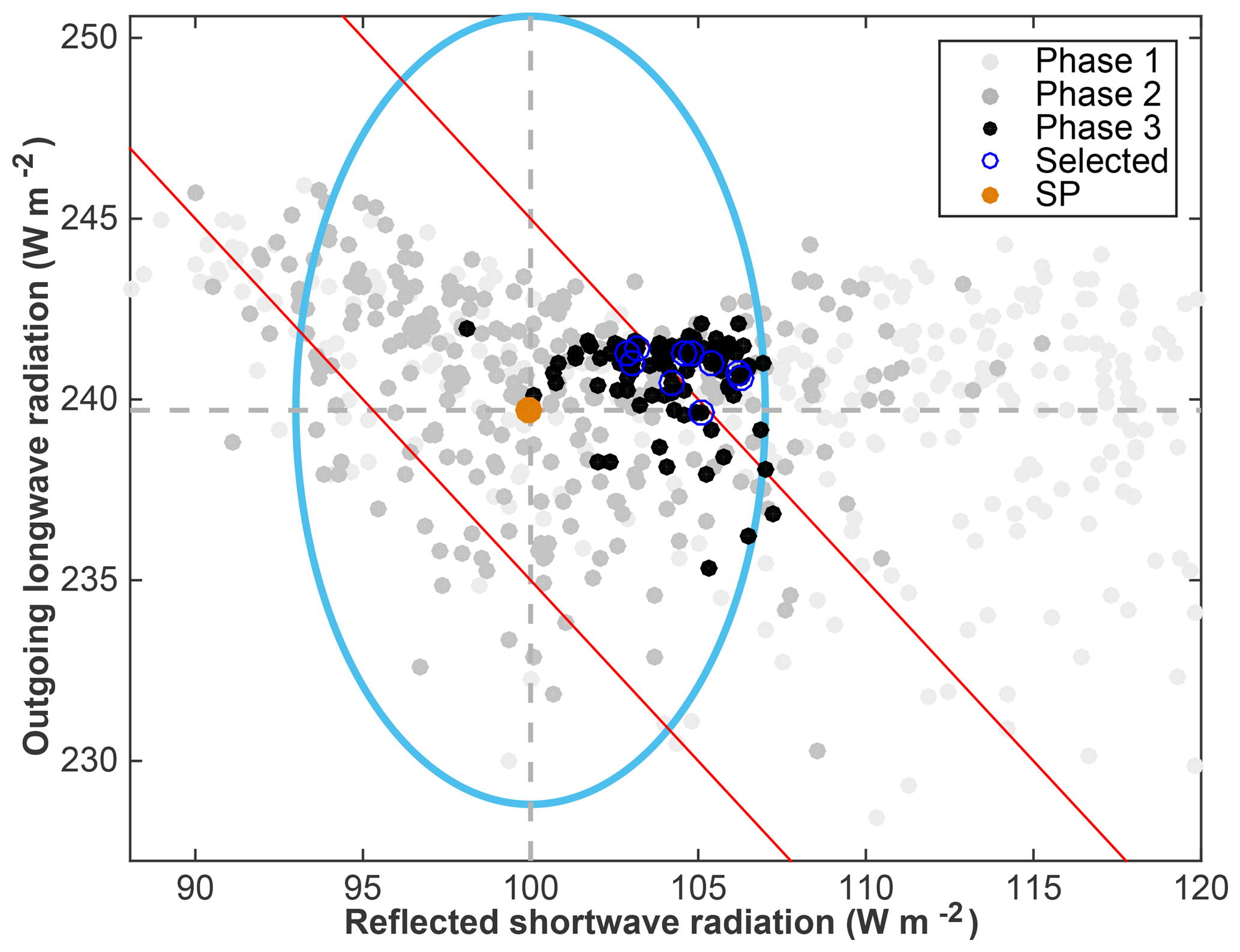
Figure 1Global mean top-of-atmosphere (TOA) outgoing (reflected) shortwave radiation (SW) and outgoing longwave radiation (LW) from the four ensembles run through weather@home2. Horizontal and vertical dashed lines denote the reference values for SW and LW taken from Stephens et al. (2012). The filled brown circle denotes our SP. The ellipse indicates the uncertainty ranges we are willing to accept for SW and LW, respectively, which includes the observational uncertainty range taken from Stephens et al. (2012), but tripled, plus the uncertainty range due to initial condition perturbations estimated from our SP reference ensemble. The red solid lines highlight net TOA energy flux of ±5 W m−2.
Rowlands et al. (2012) discarded any ensemble member that required a global annual mean flux adjustment of absolute magnitude greater than 5 W m−2 (see red lines in Fig. 1), and Yamazki et al. (2013) defined a confidence region (SW, LW) that corresponded to a TOA imbalance of less than 5 W m−2 as one that did “not drift significantly” from a realistic TOA state. Although the ranges of acceptability (Fig. 1) permits net TOA imbalance greater than 5 W m−2, more than half (55.8 %) of the Phase 3 parameter sets generated a TOA imbalance less than 5 W m−2, and the smallest TOA imbalance was less than 0.1 W m−2.
The entrainment coefficient (ENTCOEF) and the ice fall speed (VF1) were the dominant controls on the TOA outgoing SW and LW fluxes, respectively (see SW and LW response to these two parameters shown in the bottom two rows of Fig. S2). Why these parameters are important becomes clear from understanding their respective roles in the climate model, especially with respect to convection and hydrometeor transport.
The atmospheric model simulates a statistical ensemble of air plumes inside each convectively unstable grid cell. On each model layer, a proportion of rising air is allowed to mix with surrounding air and vice versa, representing the process of the turbulent entrainment of air into convection and the detrainment of air out of the convective plumes (Gregory and Rowntree, 1990). The rate at which these processes occur in the model is proportional to ENTCOEF, which is a parameter in the model convection component (Table 1). The implication of perturbing ENTCOEF has been investigated by Sanderson et al. (2008b) using single perturbation experiments, and they showed that a low ENTCOEF leads to a drier middle troposphere and moister upper troposphere. Conversely, increasing ENTCOEF results in increased low-level moisture (more low-level clouds) and decreased high-level moisture (fewer high-level clouds). Because the albedo effects of low clouds dominate their effects on emitted thermal radiation (Hartmann et al., 1992; Stephens, 2005), increasing ENTCOEF increases the outgoing SW fluxes.
VF1 is the speed at which ice particles may fall in clouds. A larger ice fall speed is associated with larger particle sizes and increased precipitation. Wu (2002) studied ice fall speed parameterization in radiative convective equilibrium models and found that a smaller ice fall speed leads to a warmer, moister atmosphere, more cloudiness, weak convection, and less precipitation, which could lead to decreased outgoing LW TOA flux due to absorption in the cloud itself and/or in the moist air. Higher ice fall speeds produce the opposite – a cooler and clearer atmosphere, less cloudiness, strong convection, and more precipitation, which increases the outgoing LW flux.
3.2 Regional climate improvements
A primary and practical purpose of climate modeling is to understand how (surface) climate will change, but model biases can have non-negligible impacts on projections. In Phases 2 and 3 we evaluate the response of regional surface climate to parameter perturbations and refine the parameter space to reduce biases in regional temperature and precipitation.
In Phase 2, we identified ENTCOEF and VF1 as distinct from the other 15 parameters with respect to their influence on the overall suite of climate metrics to a first-order approximation (Fig. S3). Recall that the regional surface metrics considered were MAC-T, JJA-T, JJA-Pr, DJF-T, and DJF-Pr. Though MAC-T is our principal metric (Sect. 2.1), MAC-T covaries with JJA-T, JJA-Pr, and DJF-T (Fig. S3), so moving in parameter space toward lower bias in MAC-T reduces biases in JJA-T, JJA-Pr, and DJF-T. MAC-T does not covary strongly with DJF-Pr.
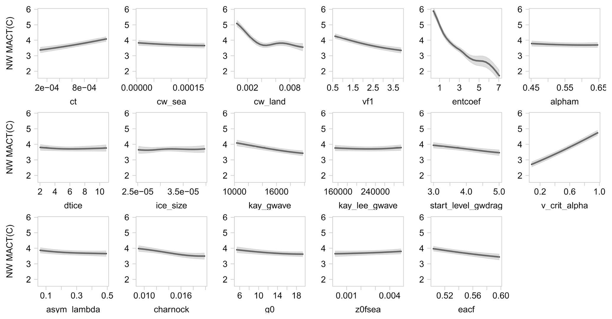
Figure 2One-at-a-time sensitivity analysis of the magnitude of the annual cycle of temperature (MAC-T) over the northwest to each input parameter in turn, with all other parameters held at the mean value of all the designed points. Heavy lines represent the emulator mean, and shaded areas represent the estimate of emulator uncertainty at the ±1 SD level.
Each OAAT relationship in Fig. 2 depends on the initial ranges of the input parameters from the ensemble design and is computed while holding all other parameters at their ensemble mean values. OAAT results while holding all other parameters at their SP values are similar to those shown in Fig. 2 (results not shown here). Because sensitivity can change as one moves through the parameter space (e.g., CW_LAND and ENTCOEF in Fig. 2), these relationships must be interpreted with care. Within the refined parameter space in Phase 2, ENTCOEF and the parameter that limits photosynthesis (and thereby latent heat flux via transpiration) as a function of soil water (V_CRIT_ALPHA) were the most influential individual parameters and counter each other when both increase (Figs. 2 and S3). The parameter that controls the cloud-droplet-to-rain threshold over land (CW_LAND) also had a strong influence on MAC-T across the lower end of the parameter perturbation range (up to 0.004). The other parameters had little to effectively no influence on MAC-T. The results of OAAT sensitivity analysis for the other output metrics considered in Phase 2 are presented in Figs. S6–S11.
The global sensitivities of the simulated outputs (the ones considered in Phase 2) due to each input, as both a main effect and total effect, including interaction terms, are presented in Fig. 3. ENTCOEF was the most important parameter for all three surface temperature metrics, with a total sensitivity index of ∼0.7, 0.5, and 0.4 for MAC-T, JJA-T, and DJF-T, respectively, wherein maximum sensitivity is 1 (see Saltelli et al., 1999). For the metrics MAC-T and JJA-T, V_CRIT_ALPHA was the next most important, with a total sensitivity index of ∼0.3 for both metrics. For JJA-Pr, the most important parameter was VF1, followed by ENTCOEF; for DJF-Pr, the most important parameter was ENTCOEF, closely followed by the parameter that controls the roughness length for free heat and moisture transport over the sea (Z0FSEA).
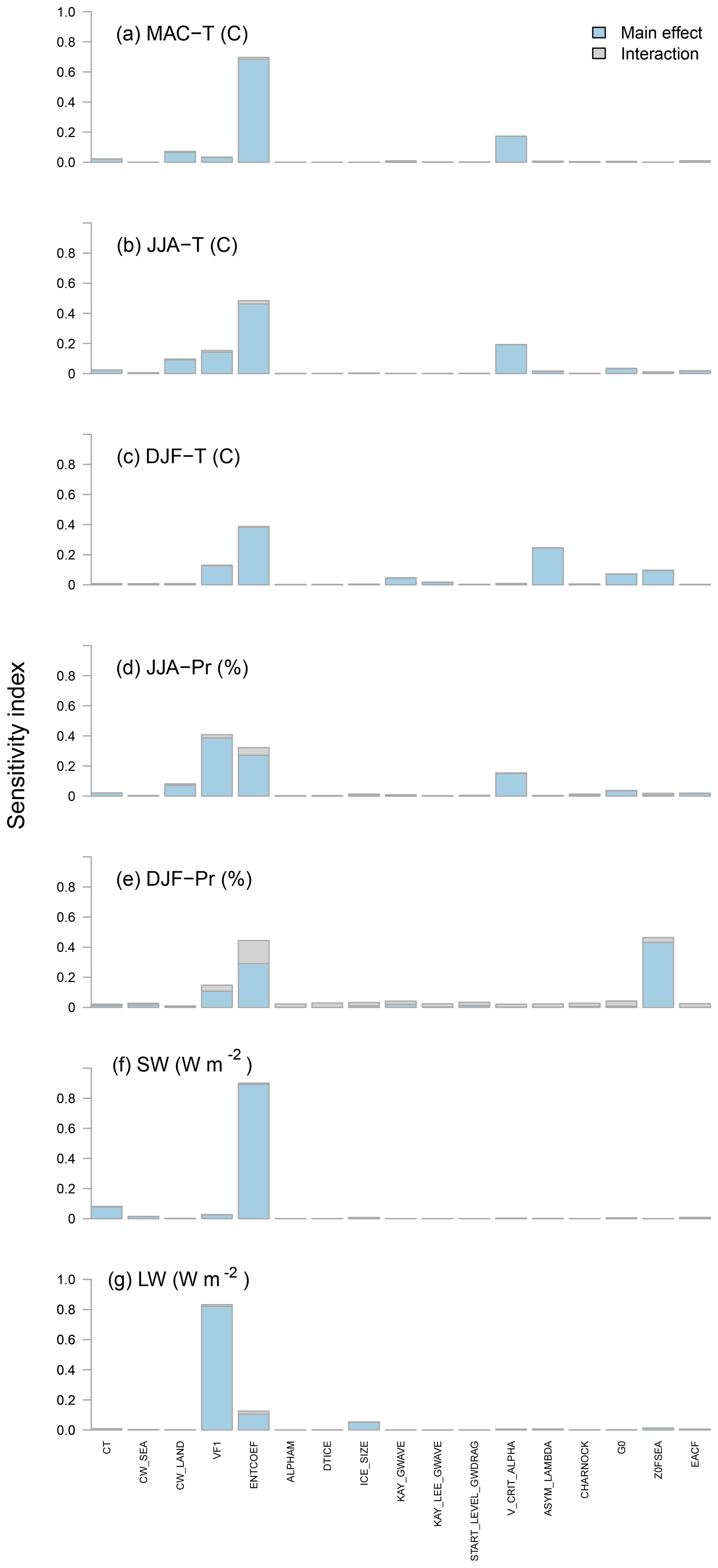
Figure 3Sensitivity analysis of model output metrics in Phase 2 via the FAST algorithm of Saltelli et al. (1999).
The interaction terms were relatively small, accounting for a few percent of the variance, except for the effect of ENTCOEF on DJF-Pr, wherein the interaction with other parameters accounts for of the variance. In a study constraining carbon cycle parameters by comparing emulator output with forest observations, McNeall et al. (2016) also found the importance of the interaction terms negligible. In contrast, Bellprat et al. (2012b) used a quadratic emulator to objectively calibrate a regional climate model and found non-negligible interaction terms. They showed that excluding the interactions in the emulator increased the error of the emulated temperature and precipitation results by almost 20 %. Further work could be done to assess the magnitude and functional form (i.e., linear or nonlinear) of the interaction terms, but this is beyond the scope of this study.
Only the parameters with a total sensitivity index larger than ∼0.1 for MAC-T, JJA-T, DJF-T, JJA-Pr, or DJF-Pr were retained for perturbation in Phase 3: CW_LAND, VF1, ENTCOEFF, V_CRIT_ALPHA, ASYM_LAMBDA, G0, and Z0FSEA. Although the parameter that controls the rate at which cloud liquid water is converted to precipitation (CT) had a total sensitivity index of ∼0.1 for SW, it was excluded from further perturbation because the primary interest in Phase 2 was in regional surface metrics, not TOA radiative fluxes.
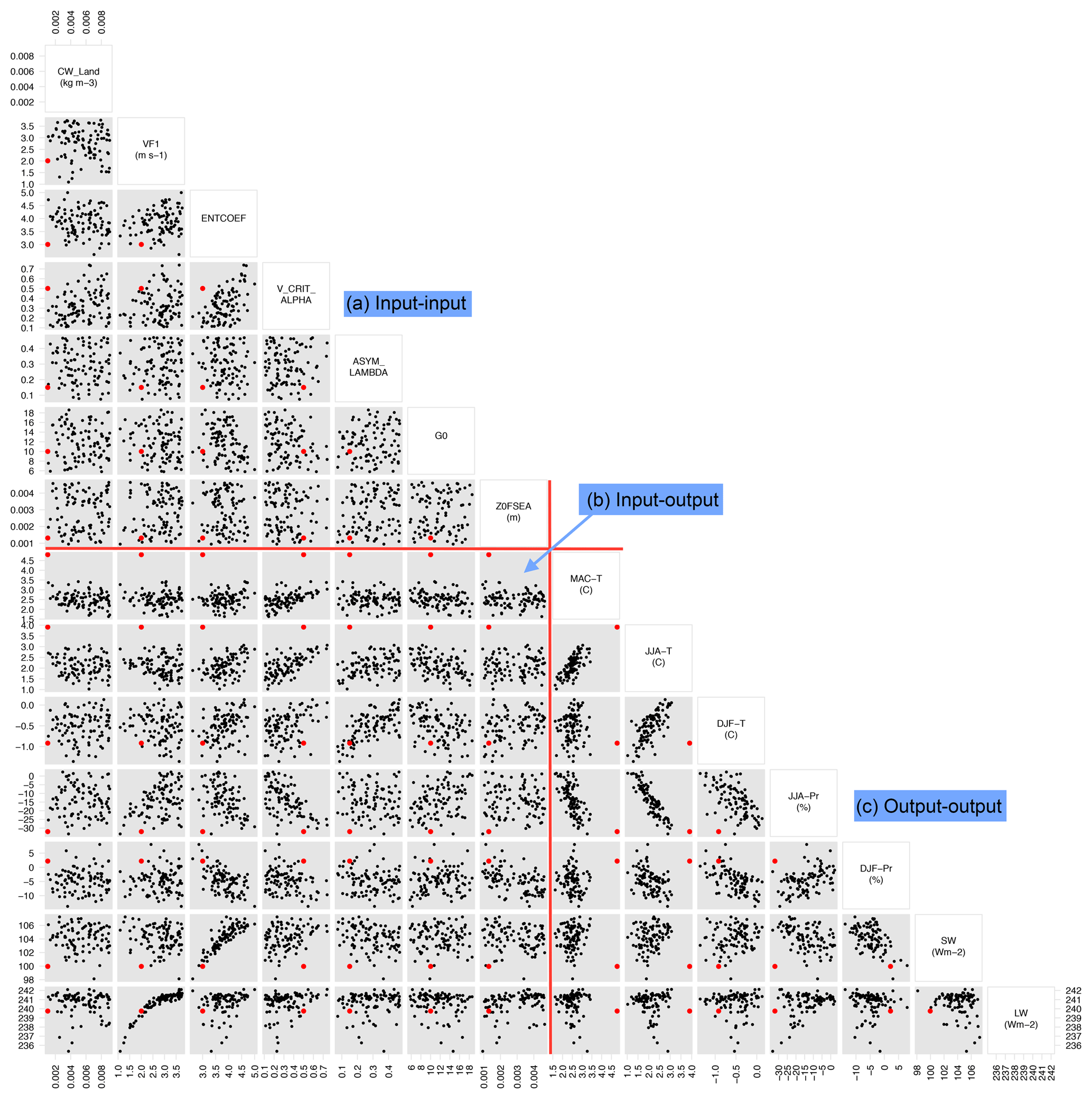
Figure 4Phase 3 PPE parameter inputs and summary model output metrics evaluated; 95 parameter sets are shown. The parameter values and model outputs under SP are marked in red. The horizontal and vertical red lines mark the transition from parameter inputs and model output metrics.
Phase 3 demonstrated the power of our approach for reducing regional mean biases in MAC-T, JJA-T, and JJA-Pr. Simulations from Phase 3 resulted in MAC-T biases 1–3 ∘C lower than SP (Fig. 4 middle row). All Phase 3 parameter sets improved the JJA-Pr dry bias, with several eliminating the bias entirely. Many parameter sets reduced the bias in JJA-T to less than 1.5 ∘C, a dramatic improvement (∼63 %) over the 4 ∘C SP bias. However, these improvements come at a small price, namely a larger regional (NWUS) dry bias in DJF-Pr (about −15 % compared with PRISM in the worst case). Because our primary goal was to reduce JJA warm and dry biases, any model variant from Phase 3 is preferable to SP. Any subset of parameterizations from Phase 3 can now be used in subsequent experiments.
V_CRIT_ALPHA plays an important role in controlling JJA-T and MAC-T (as shown in Figs. 2 and S6) due to its role in the surface hydrological budget. V_CRIT_ALPHA defines the critical point as a fraction of the difference between the wilting soil water content and the saturated soil water content (as described in Appendix C). The critical point is the soil moisture content below which plant photosynthesis becomes limited by soil water availability. When V_CRIT_ALPHA is 0, transpiration starts to be limited as soon as the soil is not completely saturated, whereas when it is 1, transpiration continues unlimited until soil moisture reaches the wilting point at which point transpiration switches off. Lower values of V_CRIT_ALPHA reduce the critical point, allowing plant photosynthesis to continue unabated at lower soil moisture levels; i.e., plants are not water-limited. As plants photosynthesize water is extracted from soil layers and transpired, increasing the local atmospheric humidity and lowering the local temperature through latent cooling. Our results are consistent with previous findings by Seneviratne et al. (2006), who also show that reducing the temperature and increasing humidity can feed back onto the regional temperature and precipitation during the summer months.
The only apparent constraints on ranges of parameter values through three phases of parameter refinement were seen for V_CRIT_ALPHA and ENTCOEF. Values of V_CRIT_ALPHA lower than 0.7 were required to keep the bias of MAC-T under 3 ∘C. For ENTCOEF, the range between 3 and 5 contains the best candidates to reduce regional warm–dry biases. The range of ENTCOEF identified here is consistent with the findings of Irvine et al. (2013), which also show that low values of ENTCOEF tend to give warmer conditions. However, results from other previous studies vary. Williamson et al. (2015) found that low values of ENTCOEF are implausible and that there are more plausible model variants at the upper end of its perturbed range, whereas Sexton et al. (2012) and Rowlands et al. (2012) consider the range between 2 and 4 to contain the best model variants. The discrepancy in optimal ranges for ENTCOEF is to be expected given that the primary metrics used to evaluate the effect of parameter refinement are different, with ours being JJA warm–dry biases over the NWUS, that of Williamson et al. (2015) being the behavior of the Antarctic Circumpolar Current, and those of other previous studies being climate sensitivities. This demonstrates that any parameter refinement process is tailored to a specific objective, and choices regarding metrics (e.g., variables, validation dataset(s), and/or cost functions) may determine which part of the parameter space is ultimately accepted.
3.3 Effects on global-scale climate
To avoid introducing or increasing biases over other parts of the globe with our regionally focused model improvement effort, we investigated the large-scale effects of the selected 10 “good” (least biased in MAC-T) sets of global parameter values. We focused on surface temperature and precipitation because they are key variables of the climate system and are of high interest for impact studies.
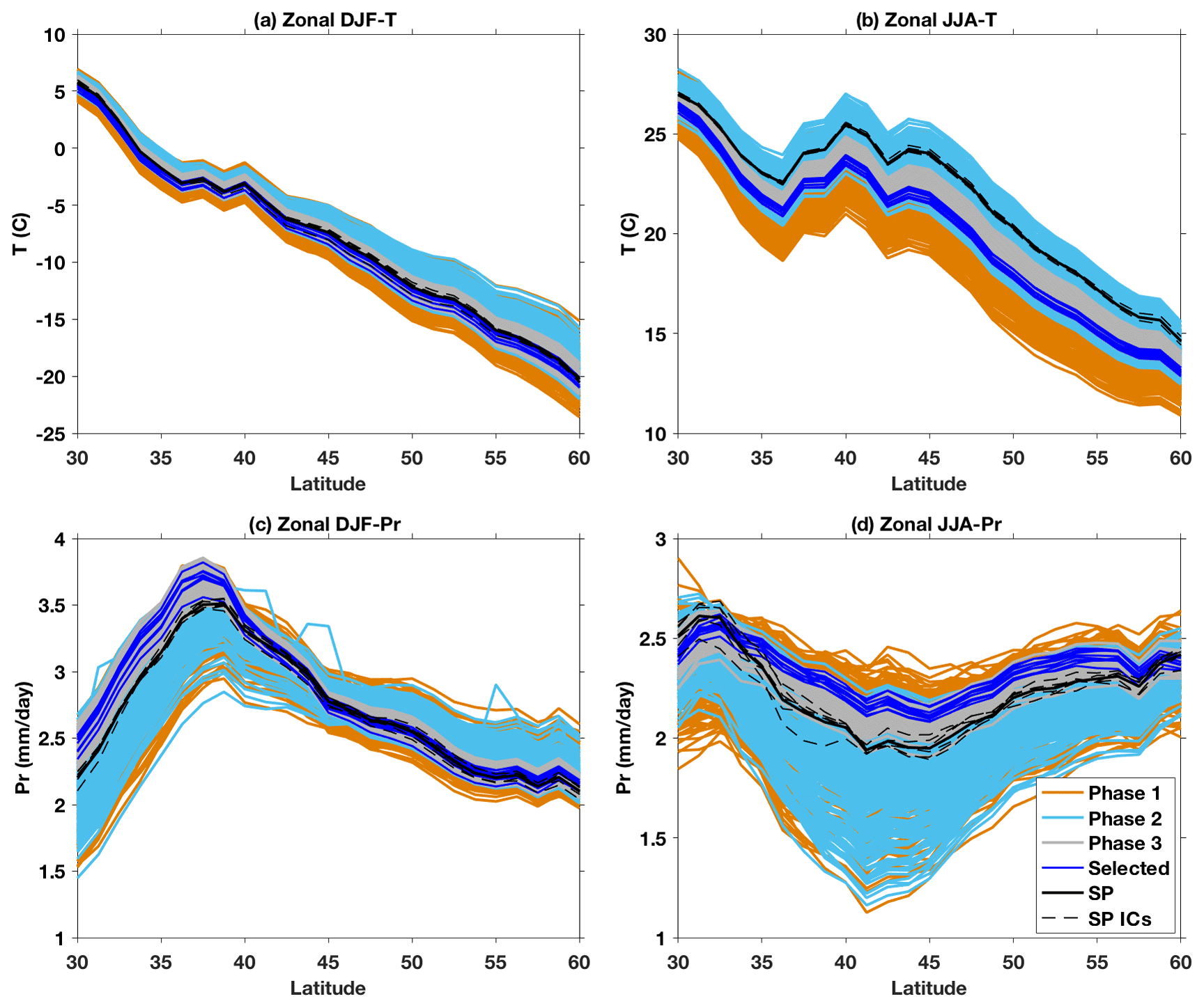
Figure 5Comparison between three PPEs and SP zonal mean HadAM3P-simulated Northern Hemisphere midlatitude (30–60∘ N) (a) DJF mean temperature over land, (b) JJA mean temperature over land, (c) DJF mean precipitation, and (d) JJA mean precipitation. Outputs from the 10 parameter sets selected, based on NWUS MAC-T, are shown in blue. Note that the plotting order is the same as the legend, so most Phase 1 curves are obscured by subsequent phases. The results from different initial conditions (ICs) under SP are shown as black dashed lines.
Figure 5 shows the meridional distribution of Northern Hemisphere (NH) midlatitude temperature (over land) and precipitation in DJF and JJA. Because of the wide range of parameter values in the PPEs of Phase 1 and Phase 2, the spread for these PPEs is quite large, whereas the ensemble spread in Phase 3 is substantially smaller. Compared with the SP ensemble, the new parameter values (final 10 sets) reduced the zonal mean JJA temperature throughout the NH midlatitudes (30–60∘ N) by ∼1–4 ∘C (depending on the particular combination of parameters) and increased JJA precipitation over the same latitude bands, except for latitudes south of 33∘ N and north of 58∘ N. In DJF, the effects are not as large nor are the changes consistent in sign across the NH midlatitude region (though south of ∼38∘ N all 10 parameter sets give increasing precipitation). The SP simulations have warm and dry biases over the NWUS and midlatitude land in general (as shown in Figs. 4, 6, and 7). In JJA all the selected PP model variants show considerably different results compared with the SP – cooler and wetter, i.e., reduced biases and improved model performance. Figure 5 also demonstrates that varying model parameters has a bigger influence than varying initial conditions, as seen from the wider spread of PP results compared with the spread of SP initial condition perturbation results.
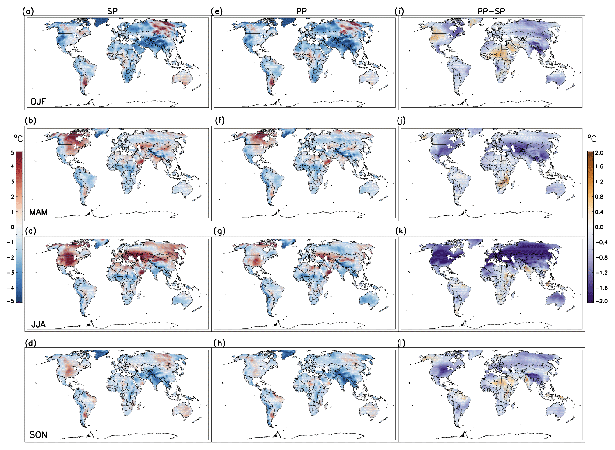
Figure 6Biases of SP temperature over land in (a) DJF, (b) MAM, (c) JJA, and (d) SON compared with CRU over December 1996 through November 2007. Biases of selected PP compared with CRU are shown in panels (e)–(h), while the differences between selected PP and SP, i.e., the absolute increase or decrease in biases in PP with respect to the SP values, are shown in panels (i)–(l). The PP results are the composites of the 10 selected sets with six ICs per set.
To examine how parameter refinements affect spatial patterns of biases, we compare the seasonal mean biases of temperature (Fig. 6) and precipitation (Fig. 7) under SP and the selected PP settings against CRU data. The SP simulations have large warm biases in JJA (and to a lesser extent in MAM and SON; Fig. 6b–d) over the NH midlatitude land region that are substantially lower in the PP simulations (Fig. 6f–h and j–l). In the tropics, the SP simulations have cold biases over northern South America, central Africa, and southern Asia in most seasons that are ameliorated in the PP simulations in some cases (e.g., central Africa in DJF and SON) – even though the focus of the PP simulations was improving the climate of the NWUS. The SP simulations also have cold biases over most of the Southern Hemisphere continents at midlatitudes in most seasons. A large fraction of the JJA temperature biases was reduced in the PP simulations, as shown in Fig. 6c, g, and k. These salient features in JJA temperature biases under SP and PP are not particular to the selection of the observational dataset (see Figs. S12–S13 for comparison with other datasets). In the other three seasons, however, the spatial patterns of temperature biases are not consistent across observational datasets.
The reduction of JJA temperature from SP to PP (Fig. 6k) and the resulting reduction in bias are accompanied by reduction in precipitation in the equatorial regions, increased precipitation over northern North America, northern Africa, and Europe (Fig. 7k), and decreased incoming shortwave radiation at the surface with increased evaporation (Fig. S14). Stronger evaporative cooling and reduced surface radiation lead to a cooling of the JJA climate, which roughly agrees with the geographical pattern of reduced mean JJA temperature, consistent with the findings in Zhang et al. (2018) that both overestimated surface shortwave radiation and underestimated evaporation contribute to the warm biases in JJA in CMIP5 climate models.
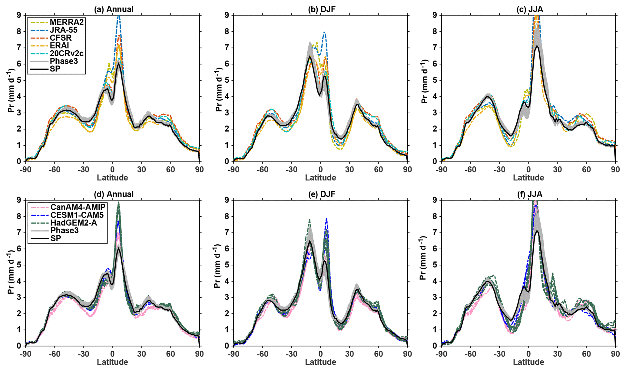
Figure 8Annual (a, d), DJF (b, e), and JJA (c, f) meridional distributions of precipitation from Phase 3 and SP (all panels). Reanalysis datasets MERRA2, JRA-55, CFSR, ERAI, and 20CRv2c are shown in panels (a–c), and GCMs CanAM4-AMIP, CESM1-CAM5, and HadGEM2-A are shown in panels (d)–(f).
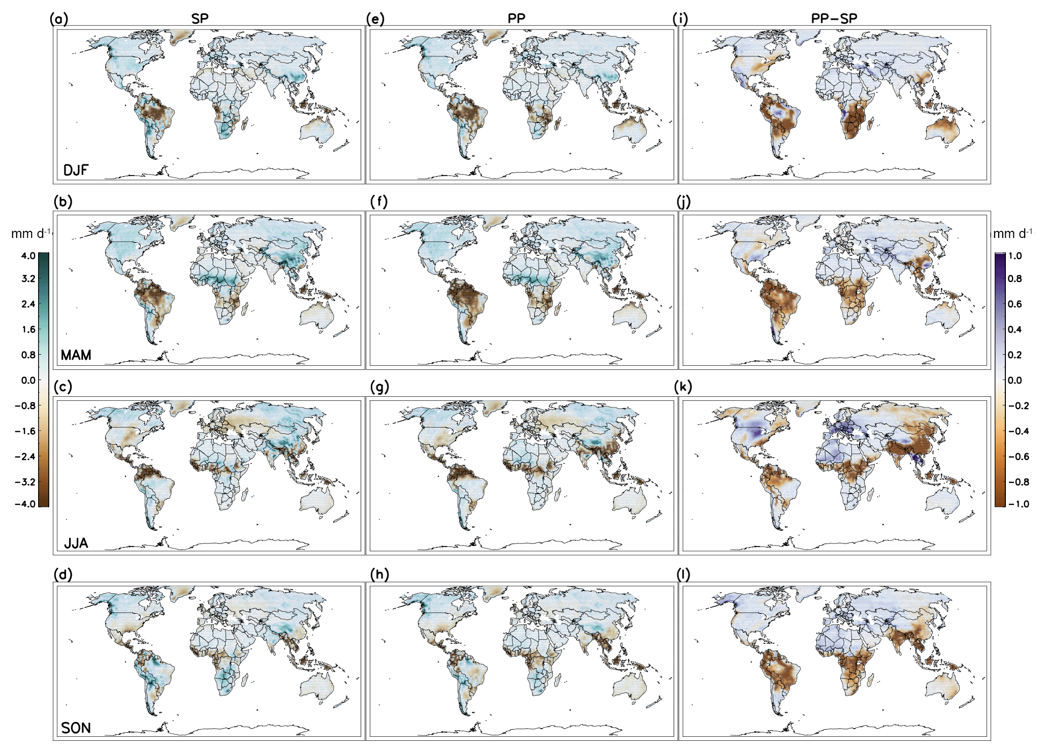
For precipitation, the largest biases in SP are over Amazonia in DJF and MAM (Fig. 7a and b) and northern South America, equatorial Africa, and south Asia in JJA (Fig. 7c). These summer biases are increased in the PP simulations (Fig. 7k). However, it is difficult to know whether we are improving the model's global precipitation patterns because of the large uncertainty in historical precipitation observational datasets. Still, it is worth comparing the PP simulations with both a variety of observational-based datasets and other GCMs (Fig. 8). The precipitation amounts differ substantially across different observational datasets, as well as across climate models. In the tropics, Phase 3 PP-simulated precipitation is mostly lower (except DJF just north of the Equator) and has a narrower range than the observations or other climate models, but it is higher in DJF and JJA (up to 25 % higher) than the SP simulation results. Outside the tropics, the precipitation distributions in PP remain similar to those of SP, and differences from observational datasets and other GCMs are less affected by the use of PP. The tropical precipitation improvements in JJA can be taken as a general improvement, though not with high confidence due to the variability across observational datasets. To further highlight the uncertainties in precipitation, global maps of differences in biases between SP and our selected parameter settings, in comparison with other observational-based datasets, are presented in Figs. S15–S22.
The fact that the large JJA warm bias (shared with many other GCMs and RCMs; see, e.g., Mearns et al., 2012; Kotlarski et al., 2014) could be reduced substantially through the use of PP is a notable result, especially since the bias persisted through initial tuning efforts and through the recent updates from version 1 to version 2 of weather@home. We demonstrated here that significant improvements in the simulation of JJA temperature can be made through parameter refinements and that these JJA temperature biases are not necessarily structural issues of the climate model. These improvements in simulating JJA temperature generally did not improve JJA precipitation patterns overall across the globe and even worsened the bias in some places (e.g., South America).
Through an iterative parameter refinement approach to improve model performance, we identified a region of climate model parameter space in which HadAM3P outperforms the SP variant in simulating summer climate over the NWUS specifically and over NH midlatitude land in general, while approximately maintaining TOA radiative (near) balance. Improving the northwest US climate comes with trade-offs, e.g., a larger JJA dry bias over Amazonia. However, it is important to note that there are large uncertainties in observed precipitation climatology, especially outside of the North American and European midlatitudes, so both apparent increases and decreases in biases should be treated with caution and compared against the range across observational datasets. In the end, we consider the cost of increasing biases in parts of the globe acceptable for the purposes of selecting multiple global model variants to drive the regional model with reduced JJA biases over the NWUS. The fact that improvements can be made at all (for a substantial area of the world) through targeted PPE is encouraging.
Our parameter refinement yielded important improvements in the representation of the summer climate over the NWUS, and it follows that biases in other models may also be reduced by refining certain parameters that, although they may not be identical to those in HadAM3–RM3P, influence the same physical processes similarly. We found ENTCOEF and V_CRIT_ALPHA to be the dominant parameters in reducing JJA biases. These parameters control cloud formation and latent heat flux, respectively. Bellprat et al. (2016) found that the key parameter responsible for the reduction of JJA biases is increased hydraulic conductivity, which increases the water availability at the land surface and leads to increased evaporative cooling, stronger low cloud formation, and associated reduced incoming shortwave radiation. We only perturbed one land surface parameter, but the effects of additional land surface parameters are being explored in a subsequent study. Given that land model parameters such as V_CRIT_ALPHA could reasonably be expected to interact with sensitive atmospheric parameters like ENTCOEF, it is particularly interesting to consider the multivariate sensitivity of a range of parameters that span across component models (e.g., land, ice, atmosphere, ocean). We argue that this frontier of parameter sensitivity should be explored in a transparent and systematic manner, and we have demonstrated that statistical emulators can be effectively leveraged to reduce computational expense.
The fact that V_CRIT_ALPHA (which is a parameter in the land surface scheme MOSES2) was found to be an important parameter in regional MAT-C and JJA-T has much further implications beyond this study. MOSES2 is the land surface scheme used in the HadGEM1 and HadGEM2 family, which were used in CMIP4 and CMIP5. Moreover, the Joint UK Land Environment Simulator (JULES) model (which is the land surface scheme of the CMIP6 generation Hadley Centre HadGEM3 family; https://www.wcrp-climate.org/wgcm-cmip/wgcm-cmip6, last access: 10 July 2019) is a development of MOSES2. What we have learned about the atmosphere–land surface interactions here is relevant to even the most recent HadGEM model generation and the in-progress CMIP6.
The reduction of JJA biases that we achieved in our multiphase parameter refinement is notable. However, despite out efforts, the “best-performing” parameter set still simulates a MAC-T bias of 1.5 ∘C and a JJA-T bias of 1 ∘C over the NWUS. Future work could be done to determine whether the model can be further improved by tuning additional land surface scheme parameters and/or to what extent the remaining biases are due to structural errors of the model for which we cannot (nor should we) compensate by refining parameter values. However, with the reduction in JJA temperature bias, future projections using the new parameter settings over the SP should be at less risk of overestimating projected warming in summer (as discussed in the Introduction).
It is also worth noting that we restricted our analysis to seasonal and annual mean climate metrics. Given the use of weather@home for attribution studies of many extreme weather events (e.g., Otto et al., 2012; Rupp et al., 2017a) as well as their impacts, such as flooding-related property damage (Schaller et al., 2016) and heat-related mortality (Mitchell et al., 2016), an important next step would be to investigate how the tails of distributions of weather variables respond to parameter perturbations. Furthermore, looking at biases in seasonal mean temperature and precipitation is insufficient to fully assess model performance. As a follow-up step to this study, we recommend a process-based model evaluation and physical explanation of model improvements to further refine the parameter space that provides improvements (e.g., reduce summer biases) through appropriate physical mechanisms. For example, a more accurate representation of clouds in the model could lead to better-simulated downward solar radiation at the surface, as well as better-simulated surface energy and water balance.
Another important next step would be to apply the selected PPE over the weather@home European domain, given the nontrivial JJA warm bias identified over Europe by previous studies (Massey et al., 2015; Sippel et al., 2016; Guillod et al., 2017). Bellprat et al. (2016) showed that regional parameters tuned over the European domain also produced similar promising results over the North American domain, but the same model parameterization yielded larger overall biases over North America than for Europe. One could test the transferability of parameter values over different regional domains in the weather@home framework, given that weather@home currently uses the same GCM to drive several RCMs over different parts of the world, all using the same parameter values.
The methodology presented in this study could be applied to other models in the evolution of physical parameterizations, and we make the argument that the parameter refinement process should be more explicit and transparent as done here. Choices and compromises made during the refinement process may significantly affect model results and influence evaluations against observed climate, and hence they should be taken into account in any interpretation of model results, especially in intercomparisons of multi-model analyses to help us understand model differences.
HadRM3P is available from the UK Met Office as part of the Providing REgional Climates for Impacts Studies (PRECIS) program. Access to the source code is dependent on attendance at a PRECIS training workshop (https://www.metoffice.gov.uk/research/applied/international/precis, last access: 10 July 2019). The code to embed the Met Office models within weather@home is proprietary and not within the scope of this publication.
The model output data for the experiment used in this study will be freely available at the Centre for Environmental Data Analysis (http://www.ceda.ac.uk, last access: 10 July 2019) in the next few months. Until the point of publication within the CEDA archive, please contact the corresponding author to access the relevant data.
The overarching goal is to refine parameter values to reduce warm and dry summer bias in the NWUS. In total four ensembles were generated, one using the SP values and one for each of three PPE phases. Details on each ensemble are listed in Table 2.
Internal variability of the atmospheric circulation can confound the relationship between parameter values and the response being sought (i.e., result in a low signal-to-noise ratio). Averaging over multiple ensemble members with the same parameter values but different atmospheric initial conditions (ICs) can clarify the true sensitivity to parameters by increasing the signal-to-noise ratio. We set up multiple ICs for each parameter set, but the numbers of ICs applied were not consistent throughout the experiment. The IC applied in each phase was determined somewhat subjectively to strike a balance between running a large enough PPE to probe as many processes and interactions between parameters as possible and to have multiple ICs so that the results were representative of the parameter perturbations instead of reflecting the influence of any particular IC while under the practical limitation of data transfer, storage, and analysis. The actual IC ensemble size used in the final analysis was also constrained by the number of successfully completed returns from the distributed computing network.
The four ensembles are summarized below.
SP. A preliminary “standard physics” (SP) ensemble with 10 ICs that used only the default model parameters was generated to provide a benchmark to access the effects of parameter perturbations.
Phase 1. The objective of this phase was to eliminate regions of parameter space that led to top-of-atmosphere (TOA) radiative fluxes that are strongly out of balance. Exclusion criteria were deliberately lenient to avoid eliminating regions of the parameter space that could potentially reproduce the observed temperature and precipitation over the western US. We perturbed 17 parameters simultaneously using space-filling Latin hypercube sampling (McKay et el., 1979) – maximizing the minimum distance between points – to generate 340 sets of parameterizations across the range of parameter values described in Table 1. To generate enough ensemble members for a statistical emulator, Loeppky et al. (2009) suggested that the number of sets of parameter values be 10 times the number of parameters (p). We used more than 10p sets of parameter values in this and subsequent phases of PPE. A total of 2040 simulations (340 sets of parameter values × 6 ICs) were submitted to the volunteer computing network. This phase was considered finalized when simulations with 220 sets of parameter values and three IC ensemble members per set were returned from the computing network.
Model results were used to train a statistical emulator that maps the relationship between parameter values and key climate metrics. In this phase, the metrics were outgoing LW and (reflected) SW TOA radiative fluxes. We considered these two metrics separately because the total net radiation could mask deficiencies in both types of radiation through cancellation of errors.
For the emulator, a two-layer feed-forward artificial neural network (ANN; Knutti et al., 2003; Sanderson et al., 2008a; Mulholland et al., 2017) was used. Although other machine-learning algorithms could be suitable (Rougier et al., 2009; Neelin et al., 2010; Bellprat et al., 2012a, b, 2016), we chose an ANN because it permits multiple simultaneous emulator targets (i.e., TOA SW and LW at the same time). We used an ellipse (Fig. 1) to define the space of acceptability for SW and LW, starting with the observational uncertainty ranges given in Stephens et al. (2012), but tripling them (deliberately setting a lenient elimination criteria), and then expanding both the negative and positive thresholds by an additional 1 W m−2 to account for internal variability as estimated from SP (Fig. S5). Sets of parameter values that fall within our range of acceptability were retained, and the ranges of these refined or restricted parameter values defined the remaining parameter space.
A new set of 1000 parameter configurations was generated from the remaining parameter space using space-filling Latin hypercube sampling. With this new ensemble we increased the sample density within the refined parameter space. The statistical emulator was used to predict SW and LW for each of these 1000 new sets of parameters, and 41 % fell within our range of acceptability, reflecting the deficiency of the emulator to some extent. Parameter sets that fell within the acceptable range were used in Phase 2.
Phase 2. The objective of this phase was to reduce biases in the simulated climate of the NWUS, where the warm summer biases were the most obvious (Fig. S1), while not straying far from TOA radiative (near) balance. The climate metrics considered were the mean magnitude of the annual cycle of temperature (MAC-T) and mean temperature (T) and precipitation (Pr) in December–January–February (DJF) and June–July–August (JJA). Although a primary motivation for this study was to investigate and reduce the warm and dry bias in JJA over the NWUS, MAC-T was treated as the primary metric in Phase 2 because it is a comprehensive measure of climate feedbacks in response to a large change in forcing, e.g., solar SW (Hall and Qu, 2006). MAC-T is also strongly correlated with the other regional metrics (particularly JJA-T) as evident in Fig. S3 – MAC-T against other metrics. We chose a NWUS average MAC-T of ±3 ∘C as the bias threshold over which parameter space would be eliminated. Though this threshold is arbitrary, falling below it would mean reducing the MAC-T bias for the NWUS by about 50 %.
We did not treat all metrics as equally important. The order of importance in this second phase was MAC-T > JJA-T, JJA-Pr, DJF-T, and DJF-Pr > SW and LW.
The 410 sets of new PPEs from Phase 1 became the starting point for Phase 2. A total of 27 060 simulations (410 sets of parameter values × 6 ICs × 11 years) was submitted to the computing network. This phase was considered finalized when simulations with 170 sets of parameter values and three IC ensemble members per set and per year were completed. These 5610 simulations were used to train a suite of statistical emulators for various climate metrics. An additional 94 sets of parameters with three IC ensemble members per set and per year completed after starting Phase 3 and were used to validate the emulators trained within Phase 2 (see Appendix B).
Separate statistical emulators were trained for MAC-T, JJA-T, JJA-Pr, DJF-T, DJF-Pr, SW, and LW. Although an ANN has the advantage of using multiple metrics as targets simultaneously, the underlying emulator structure remains obscure because an ANN is a network of simple elements called neutrons that are organized in multilayers, and different layers may perform different kinds of transformations on the inputs. For the sake of simplicity and transparency, in Phase 2 we used kriging instead – which is similar to a Gaussian process regression emulator – following McNeall et al. (2016) as coded in the package DiceKriging (Roustant et al., 2012) in the statistical programming environment R. We used universal kriging, with no “nugget” term, meaning that the uncertainty on model outputs shrinks to zero at the parameter input points that have already been run through our climate model (Roustant et al., 2012). To determine whether the emulators were adequate to predict outputs at unseen parameter inputs, we needed to ensure that it predicted relatively well across our designed parameter inputs. For each emulator, we performed “leave-one-out” cross-validation. The cross-validation results showed no significant deviations in the prediction of the outputs (results not shown).
In addition to reducing parameter space in Phase 2, we also looked for parameters that consistently showed little influence on our metrics of interest, as any reduction in parameters could benefit subsequent experiments by reducing the overall dimensionality. To identify which parameters have the most influence over the metrics of interest, we performed two types of sensitivity analyses as described in Sect. 2.5. In the end, the seven most influential parameters were retained after parameter reduction in Phase 2; these are the bold-faced parameters in Table 1.
After eliminating parameter space resulting in MAC-T biases larger than 3 ∘C and reducing the number of perturbed parameters to seven, we continued the parameter refinement process and randomly selected 100 parameter sets that emulated MAC-T biases less than 3 ∘C and had large spread in ENTCOEF and VIF1 (within the refined ranges of Phase 2). As a cutoff number of new PPE sets to run through weather@home in the next phase, 100 was subjectively chosen, mainly due to not knowing how many more phases would be required to reach our goal, while recognizing the practical constraints posed by the large datasets that would potentially be generated in the following phases.
Phase 3. This objective of this phase was to further refine parameter space to reach the target of the northwest US regional bias in MAC-T less than 3 ∘C and then select 10 sets of parameter values that met this criterion. The results in this phase satisfied our target, so we stopped the iterative process here.
We were aware that our approach of regionally targeted parameter refinements might degrade model performance elsewhere. Upon achieving our regional target, we investigated the effects of our model tuning on global model metrics.
We used 94 additional ensemble members returned from Phase 2 (the 94 simulations that completed after building the emulators from the Phase 2 PPE and starting Phase 3) to provide out-of-sample validations of the emulators trained in Phase 2. In Fig. B1, we show predictions from emulators against model-simulated values for all the output metrics. In all cases, the linear relationship between the emulated and simulated results is very strong (regression coefficient regcoef >0.9), while the emulated results can predict the simulated results relative well, with a coefficient of determination R2 >0.9 in the best cases (SW, LW, and JJA-T). It is not surprising that R2 for DJF-Pr is the smallest considering that precipitation in DJF over the NWUS is dominated by larger-scale atmospheric features such as the polar jet stream, the Pacific subtropical high, and storm tracks (e.g., Mock, 1996; Neelin et al., 2013; Seager et al., 2014; Langenbrunner et al., 2015); the internal variability of this metric is also the highest among those considered.
In Fig. B2, we present the emulated vs. simulated results in Phase 3 for the 95 PP sets that were returned in Phase 3. These 95 PP sets were run through the emulators from Phase 2 to predict the climate metrics, then the emulated results were compared with the simulated results returned from weather@home simulations. In most cases, r and R2 are lower than the Phase 2 results (Fig. B1), except for LW and DJF-T, wherein R2 increases by a few percent. This decrease in emulator prediction accuracy could be due to the fact that in Phase 3, only seven parameters were perturbed simultaneously while keeping the rest at their default values, so we have eliminated parts of the parameter space that are no longer available to the emulators.
The comparisons between simulated and emulated results from Phase 2 to Phase 3 highlight the necessity of doing parameter refinement exercise in phases. Training a statistical emulator once and then using it to search for optimal parameter settings may not always yield optimum results. An emulator may not fully capture the behavior of the climate model in every aspect, especially when the number of parameters perturbed was changed during the process, such as in our case.
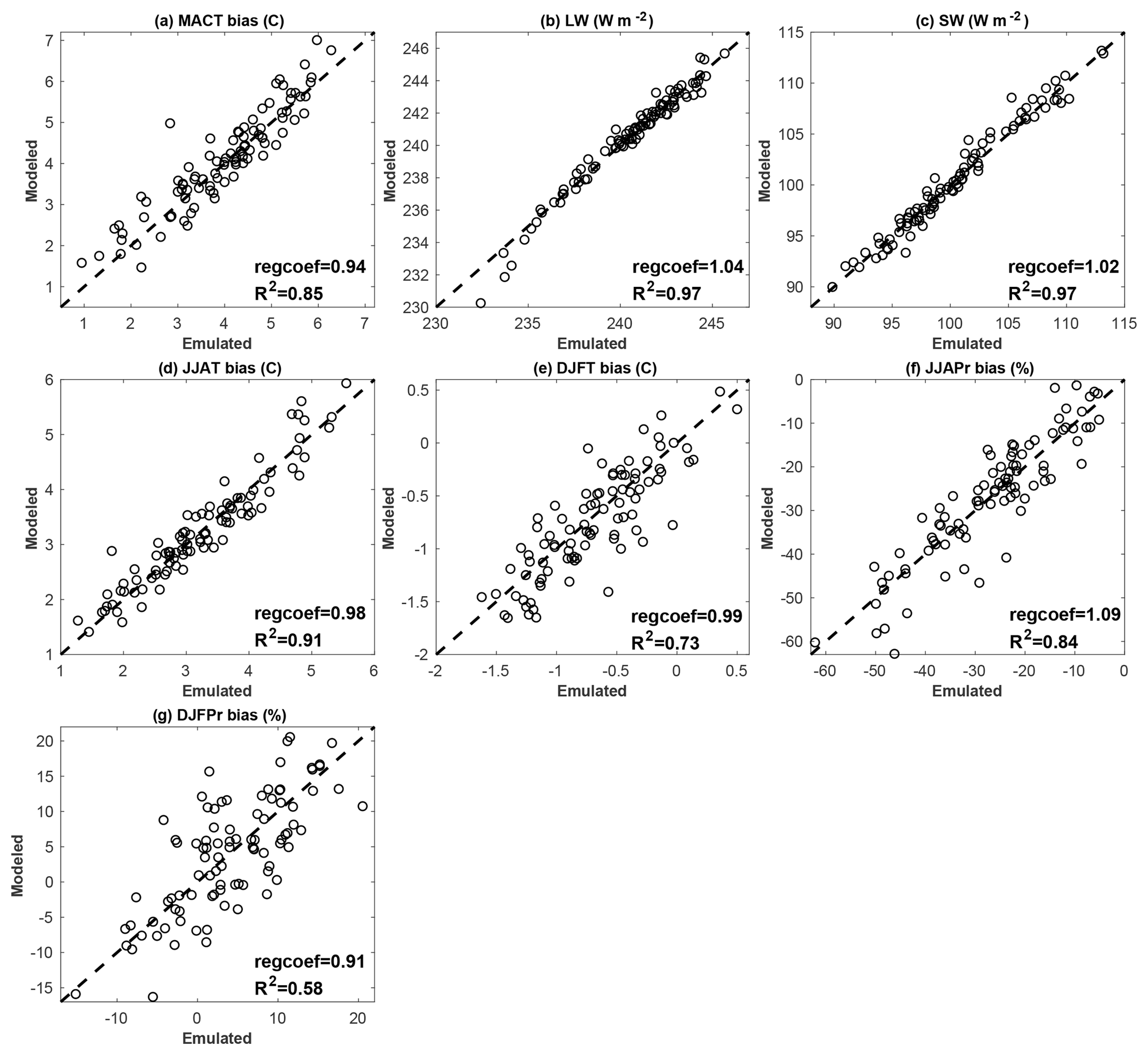
Figure B1Emulator-predicted results vs. model-simulated results in Phase 2 for different model output metrics based on 94 parameter sets not used to train the emulator (the 94 sets that finished after starting Phase 3). The regression coefficient (regcoef) and coefficient of determination (R2) from emulated results are shown in each panel. The dashed line in each panel denotes the 1 : 1 line.

Figure B2Same as Fig. B1, but for the 95 parameter sets in Phase 3. Note that the ranges of the x and y axis are set to be the same as in Fig. B1.
The critical point θcrit (cubic meters of water per cubic meters of soil) is the soil moisture content below which plant photosynthesis becomes limited by soil water availability and is calculated by
where θsat is the saturation point, i.e., the soil moisture content at the point of saturation, and θwilt is the wilting point, below which leaf stomata close. V_CRIT_ALPHA varies between 0 and 1, meaning that θcrit varies between θwilt and θsat (Cox et al., 1999).
The supplement related to this article is available online at: https://doi.org/10.5194/gmd-12-3017-2019-supplement.
The model simulations were designed by SL, DER, and LH, with inputs from PWM and DM. All the results were analyzed and plotted by SL. The paper was written by SL, with edits from DER, LH, PWM, DM, SNS, DCHW, RAB, and JJW.
The authors declare that they have no conflict of interest.
We would like to thank our colleagues at the Oxford e-Research Centre for their technical expertise. We would also like to thank the Met Office Hadley Centre PRECIS team for their technical and scientific support for the development and application of weather@home. Finally, we would like to thank all of the volunteers who have donated their computing time to climateprediction.net and weather@home.
This research has been supported by the USDA NIFA (grant no. 2013-67003-20652), Graduate School of Oregon State University, and RCUK Open Access Block Grant.
This paper was edited by James Annan and reviewed by two anonymous referees.
Adler, R. F., Huffman, G. J., Chang, A., Ferraro, R., Xie, P. P., Janowiak, J., Rudolf, B., Schneider, U., Curtis, S., Bolvin, D., Gruber, A., Susskind, J., Arkin, P., and Nelkin, E.: The Version 2 Global Precipitation Climatology Project (GPCP) Monthly Precipitation Analysis (1979-0Present), J. Hydrometeor., 4, 1147–1167, https://doi.org/10.1175/1525-7541(2003)004<1147:TVGPCP>2.0.CO;2, 2003.
Allen, M.: Do-it-yourself climate prediction, Nature, 401, 642, https://doi.org/10.1038/44266, 1999.
Annan, J. D. and Hargreaves, J. C.: Efficient estimation and ensemble generation in climate modelling, Philos. T. Roy. Soc. A, 365, 2077–2088, 2007.
Annan, J. D., Lunt, D. J., Hargreaves, J. C., and Valdes, P. J.: Parameter estimation in an atmospheric GCM using the Ensemble Kalman Filter, Nonlin. Processes Geophys., 12, 363–371, https://doi.org/10.5194/npg-12-363-2005, 2005.
Bellprat, O., Kotlarski, S., Lüthi, D., and Schär, C.: Exploring perturbed physics ensembles in a regional climate model, J. Climate, 25, 4582–4599, https://doi.org/10.1175/JCLI-D-11-00275.1, 2012a.
Bellprat, O., Kotlarski, S., Lüthi, D., and Schär, C.: Objective calibration of regional climate models, J. Geophys. Res.-Atmos., 117, D23115, https://doi.org/10.1029/2012JD018262, 2012b.
Bellprat, O., Kotlarski, S., Lüthi, D., De Elía, R., Frigon, A., Laprise, R., and Schär, C.: Objective calibration of regional climate models: application over Europe and North America, J. Climate, 29, 819–838, https://doi.org/10.1175/JCLI-D-15-0302.1, 2016.
Boberg, F. and Christensen, J. H.: Overestimation of Mediterranean summer temperature projections due to model deficiencies, Nat. Clim. Change, 2, 433–436, https://doi.org/10.1038/nclimate1454, 2012.
Booth, B. B. B., Jones, C. D., Collins, M., Totterdell, I. J., Cox, P. M., Sitch, S., Huntingford, C., Betts, R. A., Harris, G. R., and Lloyd, J.: High sensitivity of future global warming to land carbon cycle processes, Environ. Res. Lett., 7, 024002, https://doi.org/10.1088/1748-9326/7/2/024002, 2012.
Brown, T. J., Hall, B. L., and Westerling, A. L.: The impact of twenty-first century climate change on wildland fire danger in the western United States: an applications perspective, Climatic Change, 62, 365–388, 2004.
Carslaw, K. S., Lee, L. A., Reddington, C. L., Pringle, K. J., Rap, A., Forster, P. M., Mann, G. W., Spracklen, D. V., Woodhouse, M. T., Regayre, L. A., and Pierce, J. R.: Large contribution of natural aerosols to uncertainty in indirect forcing, Nature, 503, 67–71, 2013.
Cheruy, F., Dufresne, J. L., Hourdin, F., and Ducharne, A.: Role of clouds and land-atmosphere coupling in midlatitude continental summer warm biases and climate change amplification in CMIP5 simulations, Geophys. Res. Lett., 41, 6493–6500, https://doi.org/10.1002/2014GL061145, 2014.
Collins, M., Booth, B. B., Harris, G. R., Murphy, J. M., Sexton, D. M., and Webb, M. J.: Towards quantifying uncertainty in transient climate change, Clim. Dynam., 27, 127–147, 2006.
Collins, M., Booth, B. B., Bhaskaran, B., Harris, G. R., Murphy, J. M., Sexton, D. M., and Webb, M. J.: Climate model errors, feedbacks and forcings: a comparison of perturbed physics and multi-model ensembles, Clim. Dynam., 36, 1737–1766, 2011.
Collins, W. J., Bellouin, N., Doutriaux-Boucher, M., Gedney, N., Hinton, T., Jones, C. D., Liddicoat, S., Martin, G., O'Connor, F., Rae, J., Senior, C., Totterdell, I., Woodward, S., Reichler, T., and Kim, J.: Evaluation of the HadGEM2 model, Hadley Cent. Tech. Note, 74, Met Office Hadley Centre, Exter, UK, 2008.
Compo, G. P., Whitaker, J. S., Sardeshmukh, P. D., Matsui, N., Allan, R. J., Yin, X., Gleason, B. E., Vose, R. S., Rutledge, G., Bessemoulin, P., Brönnimann, S., Brunet, M., Crouthamel, R. I., Grant, A. N., Groisman, P. Y., Jones, P. D., Kruk, M. C., Kruger, A. C., Marshall, G. J., Maugeri, M., Mok, H. Y., Nordli, Ø., Ross, T. F., Trigo, R. M., Wang, X. L., Woodruff, S. D., and Worley, S. J.: The Twentieth Century Reanalysis Project, Q. J. Roy. Meteor. Soc., 137, 1–28, https://doi.org/10.1002/qj.776, 2011.
Cox, P. M., Betts, R. A., Bunton, C. B., Essery, R. L. H., Rowntree, P. R., and Smith, J.: The impact of new land surface physics on the GCM simulation of climate and climate sensitivity, Clim. Dynam., 15, 183–203, 1999.
Daly, C., Halbleib, M., Smith, J. I., Gibson, W. P., Doggett, M. K., Taylor, G. H., Curtis, J., and Pasteris, P. P.: Physiographically sensitive mapping of climatological temperature and precipitation across the conterminous United States, Int. J. Climatol., 28, 2031–2064, 2008.
Dee, D. P., Uppala, S. M., Simmons, A. J., Berrisford, P., Poli, P., Kobayashi, S., Andrae, U., Balmaseda, M. A., Balsamo, G., Bauer, P., Bechtold, P., Beljaars, A. C. M., van de Berg, L., Bidlot, J., Bormann, N., Delsol, C., Dragani, R., Fuentes, M., Geer, A. J., Haimberger, L., Healy, S. B., Hersbach, H., Hólm, E. V., Isaksen, L., Kållberg, P., Köhler, M., Matricardi, M., McNally, A. P., Monge-Sanz, B. M., Morcrette, J. J., Park, B. K., Peubey, C., de Rosnay, P., Tavolato, C., Thépaut, J. N., and Vitart, F.: The ERA-Interim reanalysis: configuration and performance of the data assimilation system, Q. J. Roy. Meteor. Soc., 137, 553–597, https://doi.org/10.1002/qj.828, 2011.
Essery, R. L. H., Best, M. J., Betts, R. A., Cox, P. M., and Taylor, C. M.: Explicit Representation of Subgrid Heterogeneity in a GCM Land Surface Scheme, J. Hydrometeorol., 4, 530–543, https://doi.org/10.1175/1525-7541(2003)004<0530:EROSHI>2.0.CO;2, 2003.
Fan, Y. and van den Dool, H.: A Global Monthly Land Surface Air Temperature Analysis for 1948–Present, J. Geophys. Res., 113, D01103, https://doi.org/10.1029/2007JD008470, 2008.
Fowler, H. J., Blenkinsop, S., and Tebaldi, C.: Linking climate change modelling to impacts studies: recent advances in downscaling techniques for hydrological modelling, Int. J. Climatol., 27, 1547–1578, 2007.
Gelaro, R., McCarty, W., Suárez, M. J., Todling, R., Molod, A., Takacs, L., Randles, C. A., Darmenov, A., Bosilovich, M. G., Reichle, R., and Wargan, K.: The modern-era retrospective analysis for research and applications, version 2 (MERRA-2), J. Climate, 30, 5419–5454, https://doi.org/10.1175/JCLI-D-16-0758.1, 2017.
Gordon, C., Cooper, C., Senior, C. A., Banks, H., Gregory, J. M., Johns, T. C., Mitchell, J. F., and Wood, R. A.: The simulation of SST, sea ice extents and ocean heat transports in a version of the Hadley Centre coupled model without flux adjustments, Clim. Dynam., 16, 147–168, 2000.
Gregory, D. and Rowntree, P. R.: A mass flux convection scheme with representation of cloud ensemble characteristics and stability-dependent closure, Mon. Weather Rev., 118, 1483–1506, 1990.
Guillod, B. P., Jones, R. G., Bowery, A., Haustein, K., Massey, N. R., Mitchell, D. M., Otto, F. E. L., Sparrow, S. N., Uhe, P., Wallom, D. C. H., Wilson, S., and Allen, M. R.: weather@home 2: validation of an improved global–regional climate modelling system, Geosci. Model Dev., 10, 1849–1872, https://doi.org/10.5194/gmd-10-1849-2017, 2017.
Guillod, B. P., Jones, R. G., Dadson, S. J., Coxon, G., Bussi, G., Freer, J., Kay, A. L., Massey, N. R., Sparrow, S. N., Wallom, D. C. H., Allen, M. R., and Hall, J. W.: A large set of potential past, present and future hydro-meteorological time series for the UK, Hydrol. Earth Syst. Sci., 22, 611–634, https://doi.org/10.5194/hess-22-611-2018, 2018.
Hall, A. and Qu, X.: Using the current seasonal cycle to constrain snow albedo feedback in future climate change, Geophys. Res. Lett., 33, L03502, https://doi.org/10.1029/2005GL025127, 2006.
Harris, G. R., Sexton, D. M., Booth, B. B., Collins, M., and Murphy, J. M.: Probabilistic projections of transient climate change, Clim. Dynam., 40, 2937–2972, 2013.
Harris, I. P. D. J., Jones, P. D., Osborn, T. J., and Lister, D. H.: Updated high-resolution grids of monthly climatic observations–the CRU TS3. 10 Dataset, Int. J. Climatol., 34, 623–642, https://doi.org/10.1002/joc.3711, 2014.
Hartmann, D. L., Ockert-Bell, M. E., and Michelsen, M. L.: The effect of cloud type on Earth's energy balance: Global analysis, J. Climate, 5, 1281–1304, https://doi.org/10.1175/1520-0442(1992)005<1281:TEOCTO>2.0.CO;2, 1992.
Hawkins, E., Osborne, T. M., Ho, C. K., and Challinor, A. J.: Calibration and bias correction of climate projections for crop modelling: an idealised case study over Europe, Agr. Forest Meteorol., 170, 19–31, 2013.
Hourdin, F., Grandpeix, J.-Y., Rio, C., Bony, S., Jam, A., Cheruy, F., Rochetin, N., Fairhead, L., Idelkadi, A., Musat, I., Dufresne, J. L., Lahellec, A., Lefebvre, M.-P., and Roehrig, R.: LMDZ5B: the atmospheric component of the IPSL climate model with revisited parameterizations for clouds and convection, Clim. Dynam., 40, 2193–2222, https://doi.org/10.1007/s00382-012-1343-y, 2013.
Huffman, G., Bolvin, D., Braithwaite, D., Hsu, K., Joyce, R., and Xie, P: Integrated Multi-satellitE Retrievals for GPM (IMERG), version 4.4. NASA's Precipitation Processing Center, available at: ftp://arthurhou.pps.eosdis.nasa.gov/gpmdata/ (last access: 31 March 2015), 2014.
Irvine, P. J., Gregoire, L. J., Lunt, D. J., and Valdes, P. J.: An efficient method to generate a perturbed parameter ensemble of a fully coupled AOGCM without flux-adjustment, Geosci. Model Dev., 6, 1447–1462, https://doi.org/10.5194/gmd-6-1447-2013, 2013.
Jackson, C., Sen, M. K., and Stoffa, P. L.: An efficient stochastic Bayesian approach to optimal parameter and uncertainty estimation for climate model predictions, J. Climate, 17, 2828–2841, 2004.
Jackson, C. S., Sen, M. K., Huerta, G., Deng, Y., and Bowman, K. P.: Error reduction and convergence in climate prediction, J. Climate, 21, 6698–6709, 2008.
Järvinen, H., Räisänen, P., Laine, M., Tamminen, J., Ilin, A., Oja, E., Solonen, A., and Haario, H.: Estimation of ECHAM5 climate model closure parameters with adaptive MCMC, Atmos. Chem. Phys., 10, 9993–10002, https://doi.org/10.5194/acp-10-9993-2010, 2010.
Johns, T. C., Durman, C. F., Banks, H. T., Roberts, M. J., McLaren, A. J., Ridley, J. K., Senior, C. A., Williams, K. D., Jones, A., Rickard, G. J., Cusack, S., Ingram, W. I., Crucifix, M., Sexton, D. M. H., Joshi, M. M., Dong, B.-W., Spencer, H., Hill, R. S. R., Gregory, J. M., Keen, A. B., Pardaens, A. K., Lowe, J. A., Bodas-Salcedo, A., Stark, S., and Searl, Y.: The new Hadley Centre climate model (HadGEM1): Evaluation of coupled simulations, J. Climate, 19, 1327–1353, https://doi.org/10.1175/JCLI3712.1, 2006.
Kalnay, E., Kanamitsu, M., Kistler, R., Collins, W., Deaven, D., Gandin, L., Iredell, M., Saha, S., White, G., Woollen, J., Zhu, Y., Chelliah, M., Ebisuzaki, W., Higgins, W., Janowiak, J., Mo, K. C., Ropelewski, C., Wang, J., Leetmaa, A., Reynolds, R., Jenne, R., and Joseph, D.: The NCEP/NCAR 40-Year Reanalysis Project, B. Am. Meteorol. Soc., 77, 437–471, 1996.
Karmalkar, A. V., Sexton, D. M., Murphy, J. M., Booth, B. B., Rostron, J. W., and McNeall, D. J.: Finding plausible and diverse variants of a climate model. Part II: development and validation of methodology, Clim. Dynam., 53, 847–877, 2019.
Knutti, R., Stocker, T. F., Joos, F., and Plattner, G. K.: Probabilistic climate change projections using neural networks, Clim. Dynam., 21, 257–272, 2003.
Kotlarski, S., Keuler, K., Christensen, O. B., Colette, A., Déqué, M., Gobiet, A., Goergen, K., Jacob, D., Lüthi, D., van Meijgaard, E., Nikulin, G., Schär, C., Teichmann, C., Vautard, R., Warrach-Sagi, K., and Wulfmeyer, V.: Regional climate modeling on European scales: a joint standard evaluation of the EURO-CORDEX RCM ensemble, Geosci. Model Dev., 7, 1297–1333, https://doi.org/10.5194/gmd-7-1297-2014, 2014.
Langenbrunner, B., Neelin, J. D., Lintner, B. R., and Anderson, B. T.: Patterns of precipitation change and climatological uncertainty among CMIP5 models, with a focus on the midlatitude Pacific storm track, J. Climate, 28, 7857–7872, 2015.
Li, S., Mote, P. W., Rupp, D. E., Vickers, D., Mera, R., and Allen, M. R.: Evaluation of a regional climate modeling effort for the western United States using a superensemble from weather@ home, J. Climate, 28, 7470–7488, 2015.
Liu, C., Ikeda, K., Rasmussen, R., Barlage, M., Newman, A. J., Prein, A. F., Chen, F., Chen, L., Clark, M., Dai, A. Dudhia, J., Eidhammer, T., Gochis, D., Gutmann, E., Kurkute, S., Li, Y., Thompson, G., and Yates, D.: Continental-scale convection-permitting modeling of the current and future climate of North America, Clim. Dynam, 49, 71–95, https://doi.org/10.1007/s00382-016-3327-9, 2017.
Loeppky, J. L., Sacks, J., and Welch, W. J.: Choosing the Sample Size of a Computer Experiment: a Practical Guide, Technometrics, 51, 366–376, 2009.
Ma, H. Y., Klein, S. A., Xie, S., Zhang, C., Tang, S., Tang, Q., Morcrette, C. J., Van Weverberg, K., Petch, J., Ahlgrimm, M., Berg, L. K., Cheruy, F., Cole, J., Forbes, R., Gustafson Jr., W. I., Huang, M., Liu, Y., Merryfield, W., Qian, Y., Roehrig, R., and Wang, Y.-C.: CAUSES: On the role of surface energy budget errors to the warm surface air temperature error over the Central United States, J. Geophys. Res.-Atmos., 123, 2888–2909, https://doi.org/10.1002/2017JD027194, 2018.
Massey, N., Jones, R., Otto, F. E. L., Aina, T., Wilson, S., Murphy, J. M., Hassell, D., Yamazaki, Y. H., and Allen, M. R.: weather@home – development and validation of a very large ensemble modelling system for probabilistic event attribution, Q. J. Roy. Meteor. Soc., 141, 1528–1545, https://doi.org/10.1002/qj.2455, 2015.
Mauritsen, T., Stevens, B., Roeckner, E., Crueger, T., Esch, M., Giorgetta, M., Haak, H., Jungclaus, J., Klocke, D., Matei, D., Mikolajewicz, U., Notz, D., Pincus, R., Schmidt, H., and Tomassini, L.: Tuning the climate of a global model, J. Adv. Model. Earth Syst., 4, M00A01, https://doi.org/10.1029/2012MS000154, 2012.
McKay, M. D., Beckman, R. J., and Conover, W. J.: Comparison of three methods for selecting values of input variables in the analysis of output from a computer code, Technometrics, 21, 239–245, 1979.
McNeall, D. J., Challenor, P. G., Gattiker, J. R., and Stone, E. J.: The potential of an observational data set for calibration of a computationally expensive computer model, Geosci. Model Dev., 6, 1715–1728, https://doi.org/10.5194/gmd-6-1715-2013, 2013.
McNeall, D., Williams, J., Booth, B., Betts, R., Challenor, P., Wiltshire, A., and Sexton, D.: The impact of structural error on parameter constraint in a climate model, Earth Syst. Dynam., 7, 917–935, https://doi.org/10.5194/esd-7-917-2016, 2016.
Mearns, L. O., Arritt, R., Biner, S., Bukovsky, M. S., McGinnis, S., Sain, S., Caya, D., Correia Jr., J., Flory, D., Gutowski, W., Takle, E. S., Jones, R., Leung, R., Moufouma-Okia, W., McDaniel, L., Nues, A. M. B., Qian, Y., Roads, J., Sloan., L., and Snyder, M.: The North American regional climate change assessment program: overview of phase I results, B. Am. Meteorol. Soc., 93, 1337–1362, 2012.
Merrifield, A. L. and Xie, S. P.: Summer US surface air temperature variability: Controlling factors and AMIP simulation biases, J. Climate, 29, 5123–5139, https://doi.org/10.1175/JCLI-D-15-0705.1, 2016.
Mitchell, D., Heaviside, C., Vardoulakis, S., Huntingford, C., Masato, G., Guillod, B. P., Frumhoff, P., Bowery, A., Wallom, D., and Allen, M.: Attributing human mortality during extreme heat waves to anthropogenic climate change, Environ. Res. Lett., 11, 074006, https://doi.org/10.1088/1748-9326/11/7/074006, 2016.
Mock, C. J.: Climatic Controls and Spatial Variations of Precipitation in the Western United States, J. Climate, 9, 1111–1125, 1996.
Morcrette, C. J., Van Weverberg, K., Ma, H. Y., Ahlgrimm, M., Bazile, E., Berg, L. K., Cheng, A., Cheruy, F., Cole, J., Forbes, R., and Gustafson Jr., W. I.: Introduction to CAUSES: Description of weather and climate models and their near-surface temperature errors in 5 day hindcasts near the Southern Great Plains, J. Geophys. Res.-Atmos., 123, 2655–2683, https://doi.org/10.1002/2017JD027199, 2018.
Mote, P. W., Allen, M. R., Jones, R. G., Li, S., Mera, R., Rupp, D. E., Salahuddin, A., and Vickers, D.: Superensemble regional climate modeling for the western United States, B. Am. Meteorol. Soc., 97, 203–215, https://doi.org/10.1175/BAMS-D-14-00090.1, 2016.
Mueller, B. and Seneviratne. S. I.: Systematic land climate and evapotranspiration biases in CMIP5 simulations, Geophys. Res. Lett., 41, 128–134, https://doi.org/10.1002/2013GL058055, 2014.
Mulholland, D. P., Haines, K., Sparrow, S. N., and Wallom, D.: Climate model forecast biases assessed with a perturbed physics ensemble, Clim. Dynam., 49, 1729–1746, 2017.
Murphy, J. M., Sexton, D. M. H., Barnett, D. N., Jones, G. S., Webb, M. J., Collins, M., and Stainforth, D. A.: Quantification of modelling uncertainties in a large ensemble of climate change simulations, Nature, 430, 768–772, https://doi.org/10.1038/nature02771, 2004.
Murphy, J. M., Booth, B. B., Collins, M., Harris, G. R., Sexton, D. M., and Webb, M. J.: A methodology for probabilistic predictions of regional climate change from perturbed physics ensembles. Philos. T. Roy. Soc. A, 365, 1993–2028, 2007.
Murphy, J. M., Sexton, D. M. H., Jenkins, G. J., Boorman, P. M., Booth, B. B. B., Brown, C. C., Clark, R. T., Collins, M., Harris, G. R., Kendon, E. J., and Betts, R. A.: UK climate projections science report: climate change projections, Met Office Hadley Centre, Exeter, UK, 21–35, 2009.
Neelin, J. D., Bracco, A., Luo, H., McWilliams, J. C., and Meyerson, J. E.: Considerations for parameter optimization and sensitivity in climate models, P. Natl. Acad. Sci. USA, 107, 21349–21354, https://doi.org/10.1073/pnas.1015473107, 2010.
Neelin, J. D., Langenbrunner, B., Meyerson, J. E., Hall, A., and Berg, N.: California winter precipitation change under global warming in the Coupled Model Intercomparison Project phase 5 ensemble, J. Climate, 26, 6238–6256, 2013.
Onogi, K., Tsutsui, J., Koide, H., Sakamoto, M., Kobayashi, S., Hatsushika, H., Matsumoto, T., Yamazaki, N., Kamahori, H., Takahashi, K., Kadokura, S., Wada, K., Kato, K., Oyama, R., Ose, T., Mannoji, N., and Taira, R.: The JRA-25 Reanalysis, J. Meteorol. Soc. Jpn., 85, 369–432, https://doi.org/10.2151/jmsj.85.369, 2007.
Otto, F. E. L., Massey, N., van Oldenborgh, G. J., Jones, R. G., and Allen, M. R.: Reconciling Two Approaches to Attribution of the 2010 Russian Heat Wave, Geophys. Res. Lett., 39, L04702, https://doi.org/10.1029/2011GL050422, 2012.
Rosenzweig, C., Elliott, J., Deryng, D., Ruane, A. C., Müller, C., Arneth, A., Boote, K. J., Folberth, C., Glotter, M., Khabarov, N., Neumann, K., Piontek, F., Pugh, T. A. M., Schmid, E., Stehfest, E., Yang, H., and Jones, J. W.: Assessing agricultural risks of climate change in the 21st century in a global gridded crop model intercomparison, P. Natl. Acad. Sci. USA, 111, 3268–3273, 2014.
Rougier, J. C., Sexton, D. M. H., Murphy, J. M., and Stainforth, D.: Analyzing the climate sensitivity of the HadSM3 climate model using ensembles from different but related experiments, J. Climate, 22, 3540–3557, https://doi.org/10.1175/2008JCLI2533.1, 2009.
Roustant, O., Ginsbourger, D., and Deville, Y.: DiceKriging, DiceOptim: Two R Packages for the Analysis of Computer Experiments by Kriging-Based Metamodeling and Optimization, J. Stat. Softw., 51, p. 54, 2012.
Rowlands, D. J., Frame, D. J., Ackerley, D., Aina, T., Booth, B. B., Christensen, C., and Gryspeerdt, E.: Broad range of 2050 warming from an observationally constrained large climate model ensemble, Nat. Geosci., 5, 256–260, 2012.
Rupp, D. E. and Li, S.: Less warming projected during heavy winter precipitation in the Cascades and Sierra Nevada, Int. J. Climatol., 37, 3984–3990, https://doi.org/10.1002/joc.4963, 2017.
Rupp, D. E., Li, S., Mote, P. W., Massey, N., Sparrow, S. N., and Wallom, D. C.: Influence of the Ocean and Greenhouse Gases on Severe Drought Likelihood in the Central US in 2012, J. Climate, 30, 1789–1806, https://doi.org/10.1175/JCLI-D-16-0294.1, 2017a.
Rupp, D. E., Li, S., Mote, P. W., Shell, K. M., Massey, N., Sparrow, S. N., Wallom, D. C. H., and Allen, M. R.: Seasonal Spatial Patterns of Projected Anthropogenic Warming in Complex Terrain: A Modeling Study of the Western USA, Clim. Dynam., 48, 2191–2213, https://doi.org/10.1007/s00382-016-3200-x, 2017b.
Saha, S., Moorthi, S., Pan, H.L., Wu, X., Wang, J., Nadiga, S., Tripp, P., Kistler, R., Woollen, J., Behringer, D., and Liu, H.: The NCEP climate forecast system reanalysis, B. Am. Meteorol. Soc., 91, 1015–1058, 2010.
Saltelli, A., Tarantola, S., and Chan, K. S.: A quantitative model-independent method for global sensitivity analysis of model output, Technometrics, 41, 39–56, 1999.
Sanderson, B. M.: A multimodel study of parametric uncertainty in predictions of climate response to rising greenhouse gas concentrations, J. Climate, 24, 1362–1377, 2011.
Sanderson, B. M., Knutti, R., Aina, T., Christensen, C., Faull, N., Frame, D. J., Ingram, W. J., Piani, C., Stainforth, D. A., Stone, D. A., and Allen, M. R.: Constraints on model response to greenhouse gas forcing and the role of subgrid-scale processes, J. Climate, 21, 2384–2400, 2008a.
Sanderson, B. M., Piani, C., Ingram, W. J., Stone, D. A., and Allen, M. R.: Towards constraining climate sensitivity by linear analysis of feedback patterns in thousands of perturbed-physics GCM simulations, Clim. Dynam., 30, 175–190, 2008b.
Sanderson, B. M., Shell, K. M., and Ingram, W.: Climate feedbacks determined using radiative kernels in a multi-thousand member ensemble of AOGCMs, Clim. Dynam., 35, 1219–1236, 2010.
Schaller, N., Kay, A. L., Lamb, R., Massey, N. R., van Oldenborgh, G. J., Otto, F. E. L., Sparrow, S. N., Vautard, R., Yiou, P., Ashpole, I., Bowery, A., Crooks, S. M., Haustein, K., Huntingford, C., Ingram, W. J., Jones, R. G., Legg, T., Miller, J., Skeggs, J., Wallom, D., Weisheimer, A., Wilson, S., Stott, P. A., and Allen, M. R.: Human Influence on Climate in the 2014 Southern England Winter Floods and Their Impacts, Nat. Clim. Change, 6, 627–634, 2016.
Schirber, S., Klocke, D., Pincus, R., Quaas, J., and Anderson, J. L.: Parameter estimation using data assimilation in an atmospheric general circulation model: From a perfect toward the real world, J. Adv. Model. Earth Syst., 5, 58–70, https://doi.org/10.1029/2012MS000167, 2013.
Schneider, U., Becker, A., Finger, P., Meyer-Christoffer, A., Rudolf, B., and Ziese, M.: GPCC Full Data Reanalysis Version 6.0 at 0.5∘: Monthly Land-Surface Precipitation from Rain-Gauges built on GTS-based and Historic Data, https://doi.org/10.5676/DWD_GPCC/FD_M_V6_050, 2011.
Seager, R., Neelin, D., Simpson, I., Liu, H., Henderson, N., Shaw, T., Kushnir, Y., Ting, M., and Cook, B.: Dynamical and thermodynamical causes of large-scale changes in the hydrological cycle over North America in response to global warming, J. Climate, 27, 7921–7948, 2014.
Seneviratne, S. I., Lüthi, D., Litschi, M., and Schär, C.: Land–atmosphere coupling and climate change in Europe, Nature, 443, 205–209, 2006.
Sexton, D. M. and Murphy, J. M.: Multivariate probabilistic projections using imperfect climate models. Part II: robustness of methodological choices and consequences for climate sensitivity, Clim. Dynam., 38, 2543–2558, 2012.
Sexton, D. M., Murphy, J. M., Collins, M., and Webb, M. J.: Multivariate probabilistic projections using imperfect climate models part I: outline of methodology, Clim. Dynam., 38, 2513–2542, 2012.
Sexton, D. M. H., Karmalkar, A. V., Murphy, J. M., Williams, K. D., Boutle, I. A., Morcrette, C. J., Stirling, A. J., and Vosper, S. B.: Finding plausible and diverse variants of a climate model. Part 1: establishing the relationship between errors at weather and climate time scales, Clim. Dynam., 53, 1–34, 2019.
Shiogama, H., Watanabe, M., Yoshimori, M., Yokohata, T., Ogura, T., Annan, J. D., Hargreaves, J. C., Abe, M., Kamae, Y., O'ishi, R., and Nobui, R.: Perturbed physics ensemble using the MIROC5 coupled atmosphere–ocean GCM without flux corrections: experimental design and results, Clim. Dynam., 39, 3041–3056, 2012.
Sippel, S., Otto, F. E. L., Forkel, M., Allen, M. R., Guillod, B. P., Heimann, M., Reichstein, M., Seneviratne, S. I., Thonicke, K., and Mahecha, M. D.: A novel bias correction methodology for climate impact simulations, Earth Syst. Dynam., 7, 71–88, https://doi.org/10.5194/esd-7-71-2016, 2016.
Solomon, S., Qin, D., Manning, M., Chen, Z., Marquis, M., Averyt, K. B., Tignor, M., and Miller, H. L.: Climate change 2007: The physical science basis, in: Contribution of Working Group I to the Fourth Assessment Report of the Intergovernmental Panel on Climate Change, 2007 Cambridge University Press, Cambridge, UK and New York, NY, USA, 2007.
Sparrow, S., Wallom, D., Mulholland, D. P., and Haines, K.: Climate model forecast biases assessed with a perturbed physics ensemble, Clim. Dynam., 49, 1729–1746, 2016.
Stainforth, D. A., Aina, T., Christensen, C., Collins, M., Faull, N., Frame, D. J., Kettleborough, J. A., Knight, S., Martin, A., Murphy, J., Piani, C., Sexton, D., Smith, L. A., Spicer, R. A., Thorpe, A. J., and Allen, M. R.: Uncertainty in predictions of the climate response to rising levels of greenhouse gases, Nature, 433, 403–406, 2005.
Stephens, G. L.: Cloud feedbacks in the climate system: A critical review, J. Climate, 18, 237–273, https://doi.org/10.1175/JCLI-3243.1, 2005.
Stephens, G. L., Li, J., Wild, M., Clayson, C. A., Loeb, N., Kato, S., L'ecuyer, T., Stackhouse Jr., P. W., Lebsock, M., and Andrews, T.: An update on Earth's energy balance in light of the latest global observations, Nat. Geosci., 5, 691–696, 2012.
Stott, P. A., Stone, D. A., and Allen, M. R.: Human contribution to the European heatwave of 2003, Nature, 432, 610–614, 2004.
Tett, S. F., Mitchell, J. F., Parker, D. E., and Allen, M. R.: Human influence on the atmospheric vertical temperature structure: Detection and observations, Science, 274, 1170–1173, 1996.
Tett, S. F. B., Yamazaki, K., Mineter, M. J., Cartis, C., and Eizenberg, N.: Calibrating climate models using inverse methods: case studies with HadAM3, HadAM3P and HadCM3, Geosci. Model Dev., 10, 3567–3589, https://doi.org/10.5194/gmd-10-3567-2017, 2017.
Uhe, P., Philip, S., Kew, S., Shah, K., Kimutai, J., Mwangi, E., van Oldenborgh, G. J., Singh, R., Arrighi, J., Jjemba, E., Cullen, H., and Otto, F. E. L.: Attributing Drivers of the 2016 Kenyan Drought, Int. J. Climatol., 38, e554–e568, 2018.
van Oldenborgh, G. J., Otto, F. E. L., Haustein, K., and AchutaRao, K.: The Heavy Precipitation Rvent of December 2015 in Chennai, India, In Explaining Extremes of 2015 from a Climate Perspective, B. Am. Meteorol. Soc., 97, S87–S91, 2016.
van Oldenborgh, G. J., van der Wiel, K., Sebastian, A., Singh, R., Arrighi, J., Otto, F. E. L., Haustein, K., Li, S., Vecchi, G., and Cullen, H.: Attribution of Extreme Rainfall from Hurricane Harvey, August 2017, Environ. Res. Lett., 12, 124009, https://doi.org/10.1088/1748-9326/aaa343, 2017.
Van Weverberg, K., Morcrette, C. J., Petch, J., Klein, S. A., Ma, H. Y., Zhang, C., Xie, S., Tang, Q., Gustafson Jr., W. I., Qian, Y., and Berg, L. K.: CAUSES: Attribution of surface radiation biases in NWP and climate models near the U.S. Southern Great Plains, J. Geophys. Res.-Atmos., 123, 3612–3644, https://doi.org/10.1002/2017JD027188, 2018.
Williams, J. H. T., Smith, R. S., Valdes, P. J., Booth, B. B. B., and Osprey, A.: Optimising the FAMOUS climate model: inclusion of global carbon cycling, Geosci. Model Dev., 6, 141–160, https://doi.org/10.5194/gmd-6-141-2013, 2013.
Williamson, D., Goldstein, M., Allison, L., Blaker, A., Challenor, P., Jackson, L., and Yamazaki, K.: History matching for exploring and reducing climate model parameter space using observations and a large perturbed physics ensemble, Clim. Dynam., 41, 1703–1729, 2013.
Williamson, D., Blaker, A. T., Hampton, C., and Salter, J.: Identifying and removing structural biases in climate models with history matching, Clim. Dynam., 45, 1299–1324, 2015.
Williamson, D. B., Blaker, A. T., and Sinha, B.: Tuning without over-tuning: parametric uncertainty quantification for the NEMO ocean model, Geosci. Model Dev., 10, 1789–1816, https://doi.org/10.5194/gmd-10-1789-2017, 2017.
Wu, X.: Effects of ice mircrophysics on tropical radiative-convective-oceanic quasi-equilibrium states, J. Atmos. Sci., 59, 1885–1897, 2002.
Xie, P. and Arkin, P. A.: Global precipitation: a 17-year monthly analysis based on gauge observations, satellite estimates, and numerical model outputs, B. Am. Meteorol. Soc., 78, 2539–2558, 1996.
Yamazaki, K., Rowlands, D. J., Aina, T., Blaker, A., Bowery, A., Massey, N., Miller, J., Rye, C., Tett, S. F. B., Williamson, D., Yamazaki, Y. H., and Allen, M. R.: Obtaining diverse behaviors in a climate model without the use of flux adjustments, J. Geophys. Res.-Atmos., 118, 2781–2793, https://doi.org/10.1002/jgrd.50304, 2013.
Zhang, C., Xie, S., Klein, S. A., Ma, H.Y ., Tang, S., Van Weverberg, K., Morcrette, C. J., and Petch, J.: CAUSES: Diagnosis of the summertime warm bias in CMIP5 climate models at the ARM Southern Great Plains site, J. Geophys. Res.-Atmos., 123, 2968–2992, https://doi.org/10.1002/2017JD027200, 2018.
Zhang, T., Li, L., Lin, Y., Xue, W., Xie, F., Xu, H., and Huang, X.: An automatic and effective parameter optimization method for model tuning, Geosci. Model Dev., 8, 3579–3591, https://doi.org/10.5194/gmd-8-3579-2015, 2015.
- Abstract
- Introduction
- Methodology
- Results and discussion
- Conclusions
- Code availability
- Data availability
- Appendix A: Detailed experimental process
- Appendix B: Emulated vs. simulated results
- Appendix C: Soil moisture control on plant photosynthesis in MOSES
- Author contributions
- Competing interests
- Acknowledgements
- Financial support
- Review statement
- References
- Supplement