A simplified parameterization of isoprene-epoxydiol-derived secondary organic aerosol (IEPOX-SOA) for global chemistry and climate models: a case study with GEOS-Chem v11-02-rc

Secondary organic aerosol derived from isoprene epoxydiols (IEPOX-SOA) is thought to contribute the dominant fraction of total isoprene SOA, but the current volatility-based lumped SOA parameterizations are not appropriate to represent the reactive uptake of IEPOX onto acidified aerosols. A full explicit modeling of this chemistry is however computationally expensive owing to the many species and reactions tracked, which makes it difficult to include it in chemistry–climate models for long-term studies. Here we present three simplified parameterizations (version 1.0) for IEPOX-SOA simulation, based on an approximate analytical/fitting solution of the IEPOX-SOA yield and formation timescale. The yield and timescale can then be directly calculated using the global model fields of oxidants, NO, aerosol pH and other key properties, and dry deposition rates. The advantage of the proposed parameterizations is that they do not require the simulation of the intermediates while retaining the key physicochemical dependencies. We have implemented the new parameterizations into the GEOS-Chem v11-02-rc chemical transport model, which has two empirical treatments for isoprene SOA (the volatility-basis-set, VBS, approach and a fixed 3 % yield parameterization), and compared all of them to the case with detailed fully explicit chemistry. The best parameterization (PAR3) captures the global tropospheric burden of IEPOX-SOA and its spatiotemporal distribution (R²=0.94) vs. those simulated by the full chemistry, while being more computationally efficient (∼5 times faster), and accurately captures the response to changes in NO_x and SO₂ emissions. On the other hand, the constant 3 % yield that is now the default in GEOS-Chem deviates strongly (R²=0.66), as does the VBS (R²=0.47, 49 % underestimation), with neither parameterization capturing the response to emission changes. With the advent of new mass spectrometry instrumentation, many detailed SOA mechanisms are being developed, which will challenge global and especially climate models with their computational cost. The methods developed in this study can be applied to other SOA pathways, which can allow including accurate SOA simulations in climate and global modeling studies in the future.

1 Introduction

Secondary organic aerosols (SOAs) are a major component of submicron particulate matter globally (Zhang et al., 2007; Jimenez et al., 2009) but are typically poorly predicted by global models (Tsigaridis et al., 2014). Isoprene is the most abundant nonmethane volatile organic compound (VOC), whose global emission flux (∼600 Tg yr⁻¹) is much larger than that of monoterpenes (∼100 Tg yr⁻¹) (Sindelarova et al., 2014) and nonmethane VOCs from anthropogenic sources (∼130 Tg yr⁻¹) (Lamarque et al., 2010). On account of its global source strength, isoprene oxidation can contribute substantially to SOA in the atmosphere, even if its yield is small (Carlton et al., 2009). There are several isoprene oxidation products that can lead to SOA formation, including isoprene-derived epoxydiols (IEPOX) (Paulot et al., 2009), glyoxal and methyl glyoxal (Fu et al., 2008), gas-phase low-volatility organic compounds (LVOC) produced from gas-phase oxidation of hydroxy hydroperoxides (ISOPOOH) (Krechmer et al., 2015; Liu et al., 2016), and methacryloylperoxynitrate (MPAN) (Surratt et al., 2010). Gas-phase IEPOX, mainly formed from the photooxidation of isoprene under low-NO conditions (Paulot et al., 2009), can efficiently partition onto aqueous acidic aerosols and produce SOA through aqueous-phase reactions (Paulot et al., 2009; Surratt et al., 2010; Gaston et al., 2014a; Zhang et al., 2018). SOA from IEPOX (IEPOX-SOA) is considered at present the dominant isoprene-derived SOA pathway (Marais et al., 2016; Carlton et al., 2018; Mao et al., 2018), compared to a less efficient formation from glyoxal (Knote et al., 2014).

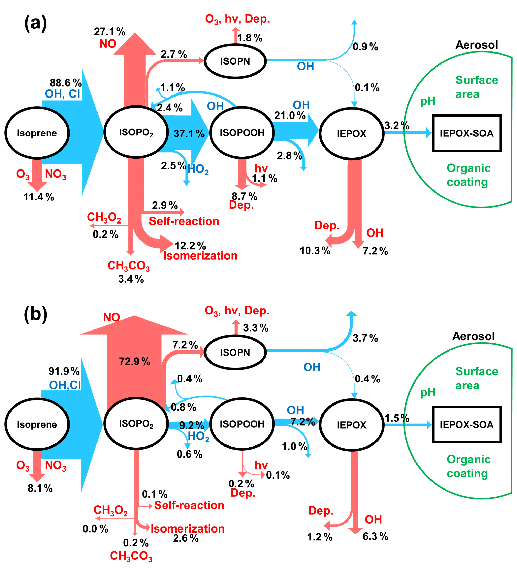
Figure 1 Schematic diagrams of IEPOX-SOA chemistry for (a) HO₂- and (b) NO-dominant regions. Blue arrows indicate IEPOX-SOA formation pathways and red arrows represent other chemical pathways that do not form significant IEPOX-SOA. “Dep.” and “hv” represent wet and dry deposition and photolytic losses, respectively. Values are averaged molar yields relative to the initial oxidation amount of isoprene from GEOS-Chem v11-02-rc results using the explicit full chemistry with updates in this study (see Sect. 2.2) over Borneo (as an example of HO₂-dominant conditions; 5^∘ S–5^∘ N, 105–120^∘ E) and Beijing (as an example of NO-dominant conditions; 35–45^∘ N, 110–120^∘ E) from July 2013 to June 2014. We note that Beijing is located in a region with typically low isoprene emissions, so the appreciable yield of IEPOX-SOA will still result in small ambient concentrations.

Ground-based and aircraft field measurements have shown that IEPOX-SOA can contribute to total OA concentrations by as much as 36 %, especially for forested regions under low NO across the globe (Hu et al., 2015). Several modeling studies have explicitly simulated IEPOX-SOA by considering detailed isoprene gas-phase chemistry and IEPOX uptake (Marais et al., 2016; Budisulistiorini et al., 2017; Stadtler et al., 2018). Figure 1 shows the main chemical pathways of the IEPOX-SOA chemistry in (a) HO₂- and (b) NO-dominant conditions simulated by GEOS-Chem. The fate of isoprene peroxy radicals (ISOPO₂) is substantially affected by the NO and HO₂ concentrations, which modulate the strength of the IEPOX-SOA pathway, consistent with observations in different regions (Hu et al., 2015). In the HO₂-dominant regions (panel a), most ISOPO₂ reacts with HO₂ to produce ISOPOOH and later IEPOX with a yield of 21.0 %. On the other hand, the IEPOX yield is lower (7.2 % here) for regions where the NO pathway is dominant (panel b). An opposite tendency is calculated for an IEPOX-SOA yield from IEPOX, implying the nonlinear chemistry by various factors. The IEPOX-SOA yields from IEPOX are 15.2 % (3.2/21.0) and 20.8 % (1.5/7.2), respectively, for (a) Borneo and (b) Beijing based on GEOS-Chem model calculations, which can be mainly explained by the higher available aerosol surface area in Beijing compared to Borneo.

Marais et al. (2016) reported that the model with the explicit irreversible uptake of isoprene SOA precursors to aqueous aerosols coupled to detailed gas-phase chemistry predicted isoprene SOA better than the default isoprene SOA mechanism based on volatility basis set (VBS) in GEOS-Chem v09-02. The VBS mechanism is based on the reversible partitioning of first-generation semivolatile oxidation products onto preexisting dry OA (Pye et al., 2010). The default VBS mechanism in GEOS-Chem underestimated the observed isoprene SOA formation by a factor of 3 over the southeast US in summer, whereas the model with the detailed isoprene chemistry showed a close agreement with the measured aircraft and surface isoprene-derived SOA concentrations.

The use of increasingly detailed chemistry in models enables realistic prediction of chemical composition in the atmosphere, but it is limited by the prohibiting computational cost. As a result, most of the models participating in the fifth phase of the Coupled Model Intercomparison Project (CMIP5) (Taylor et al., 2011), which provided results for the recent IPCC report (Stocker et al., 2013), used very simplified approaches, such as assuming that a constant fraction of emissions occur as nonvolatile SOA (Tsigaridis and Kanakidou, 2018). These simplified approaches were also used in many models participating in the recent AeroCom intercomparison study of OA (Tsigaridis et al., 2014). The modeling community has tried to improve computational efficiency by condensing complex VBS schemes into simpler ones (Shrivastava et al., 2011; Koo et al., 2014) or by developing empirical parameterizations based on field observations (Hodzic and Jimenez, 2011; Kim et al., 2015). In order to avoid the extra computational cost of the full isoprene mechanism, GEOS-Chem v11-02-rc includes a fixed 3 % yield of SOA from isoprene emission for most model applications based on the study by Kim et al. (2015) and confirmed by the study with the explicit isoprene SOA mechanism in Marais et al. (2016). However, the 3 % yield was derived from the measurements over the southeast US during summer in 2013 (Marais et al., 2016), but the explicit isoprene SOA mechanism estimated a wide range of SOA yields (3 %–13 %) in different years (Marais et al., 2017), implying that isoprene SOA yields could be different under different physicochemical environments in other regions and time periods (Hu et al., 2015).

In this study, we develop IEPOX-SOA parameterizations based on approximate analytical solutions of the relevant portion of the isoprene chemical mechanism supplemented with numerical fitting. First, a box model is used to develop and evaluate the parameterizations. We then implement the parameterizations into GEOS-Chem and compare the results against those from the explicit irreversible uptake of isoprene SOA precursors to aqueous aerosols coupled to detailed gas-phase chemistry, the default fixed 3 % yield, and the VBS scheme. We investigate the performance and limitations of the new parameterizations in terms of global tropospheric concentrations, vertical profiles, and burdens. Our methods substantially reduce the computational cost of the explicit isoprene SOA mechanism and provide a much-improved simulation compared to the fixed 3 % yield and the VBS parameterizations.

2 Global model description

2.1 General

We used the GEOS-Chem (v11-02-rc) global 3-D chemical transport model (Bey et al., 2001) to run the parameterizations described in Sect. 3, as well as the explicit isoprene SOA mechanism, fixed 3 % yield, and VBS schemes. The model was driven by Goddard Earth Observing System Forward Processing (GEOS-FP) assimilated meteorological data from the NASA Global Modeling and Assimilation Office (GMAO) for a year (July 2013 to June 2014) with a spin-up time of 2 months. Winds, temperature, precipitation, and other meteorological variables are provided at 0.3125^∘ (longitude) × 0.25^∘ (latitude) and regridded to 2.5^∘ (longitude) × 2^∘ (latitude) for computational efficiency. GEOS-Chem simulates gas-phase chemistry and aerosol formation including sulfate, ammonium, nitrate (Park et al., 2006), black carbon (Park et al., 2003), OA (Pye et al., 2010; Kim et al., 2015; Marais et al., 2016), sea salt (Jaeglé et al., 2011), and dust (Fairlie et al., 2007). Gas–particle partitioning of inorganic aerosols and aerosol pH are computed with the ISORROPIA II thermodynamic model (Fountoukis and Nenes, 2007; Pye et al., 2009).

2.2 Update to the full mechanism of IEPOX-SOA uptake

We updated the standard mechanism and code of GEOS-Chem v11-02-rc to include two recent scientific findings influencing the IEPOX-SOA uptake rate. First, we considered organic coating effects when we calculated reactive IEPOX uptake by assuming core (inorganic) and shell (organic) mixing state (Zhang et al., 2018). The detailed information for the register model and parameters used in this study are given in Sect. S1 in the Supplement.

Standard GEOS-Chem assumes no organic coating, only the surface area of inorganic aerosols. We updated the model to include suppression of IEPOX reactive uptake by the organic coating and to use the available surface area of the total sulfate–ammonium–nitrate–organic-aerosol mixture at a given relative humidity with hygroscopic growth factors. We found that the IEPOX reactive uptake coefficient (γ) was always decreased at atmospheric relevant aerosol pH and relative humidity conditions, but the IEPOX reactive uptake rate constant increased in some conditions (high pH and high IEPOX diffusion coefficient in the organic layer, Fig. S2 in the Supplement). We note that this is the case for GEOS-Chem v11-02-rc, because GEOS-Chem does not take into account organic aerosol mass for aerosol radius and aerosol surface area calculation when it calculates IEPOX reactive uptake. Therefore, additional OA mass considered in this study increases available aerosol surface area for IEPOX reactive uptake, which compensates or sometimes overcomes the effects by the decrease of γ as shown in Eq. (1) for the first-order uptake rate constant of IEPOX to form IEPOX-SOA:

$$\begin{array}{}\text{(1)}& \mathrm{IEPOX}\mathrm{uptake}\mathrm{rate}\mathrm{constant}={\displaystyle \frac{S_{\mathrm{a}}}{\frac{r_{\mathrm{a}}}{D_{\mathrm{g}}}+\frac{\mathrm{4}}{\mathit{\gamma }\times v_{\mathrm{mms}}}}}.\end{array}$$

S_a is the wet aerosol surface area on which IEPOX can be taken up (m² m⁻³), r_a is the wet aerosol radius (m), D_g is gas-phase diffusion coefficient of IEPOX (m² s⁻¹), and v_mms is the mean molecular speed (m s⁻¹) of gas-phase IEPOX. Again, the effects of organic coating on the IEPOX uptake rate constant in this study can be different from previous observational studies (Hu et al., 2016; Zhang et al., 2018), because observational studies used the measured and fixed available aerosol surface area and radius, and they changed organic aerosol layer thickness for their calculations (i.e., inorganic core radius was changed, but total particle radius and surface area were not changed). When we assumed the fixed aerosol radius and aerosol surface area, and only organic coating thickness increased as OA mass increased as per previous observational studies, all the cases showed the decreasing IEPOX reactive uptake rate constants (Fig. S3).

Parameters used in this study such as the Henry's law constant and the IEPOX diffusion coefficient in OA can be easily updated in future studies, as new information becomes available in the literature. Our parameterizations are flexible to the change in these variables, because they use the IEPOX reactive uptake rate constant (k₁₈ in Eqs. 7 and 14 in Sect. 3) rather than using individual input parameters. Therefore, updating the parameterizations developed here with more accurate values of input parameters determined in future literature studies is easy without having to refit the parameterizations.

Second, we calculate the submicron aerosol pH without sea salt based on the results from previous studies (Noble and Prather, 1996; Middlebrook et al., 2003; Hatch et al., 2011; Allen et al., 2015; Guo et al., 2016; Bondy et al., 2018; Murphy et al., 2019), which showed that sea salt aerosols were dominantly externally mixed with sulfate–nitrate–ammonium rather than internally mixed. Therefore, sea salt is not expected to impact submicron aerosol pH significantly in the real atmosphere. Effects of sea salt on pH and detailed analysis against the aircraft measurements were discussed in detail by Nault et al. (2018).

2.3 Isoprene SOA simulations

In this section, we briefly describe three different schemes for isoprene SOA simulations used in GEOS-Chem v11-02-rc: the explicit scheme (Marais et al., 2016), the VBS (Pye et al., 2010), and the fixed 3 % parameterization (Kim et al., 2015). In the explicit scheme, isoprene and its products, as well as related processes including chemistry, dry and wet deposition, and transport, are explicitly calculated in GEOS-Chem. The chemical mechanism related to IEPOX-SOA formation is shown in Table S1. Gas-phase concentrations of isoprene, ISOPO₂, ISOPOOH, IEPOX, and isoprene nitrate (ISOPN) are explicitly calculated in every model grid point. All the species (except for ISOPO₂ because of its short lifetime) are transported in the model. More detailed information can be found in Marais et al. (2016), with some updates for isomer reactions described in Sect. 3.1.

The VBS scheme implemented in GEOS-Chem uses six tracers to simulate isoprene SOA, three for gas-phase and three for aerosol-phase concentrations. This scheme calculates semivolatile products from the isoprene + OH reaction and distributes them into three saturation vapor pressure bins ($C^{\ast }=\mathrm{1}$, 10, 100 µg m⁻³). These products are partitioned into gas (ISOG1–3 in GEOS-Chem) and aerosol phase (ISOA1–3 in GEOS-Chem) at every model time step based on equilibrium partitioning (Pankow, 1994). Dry and wet deposition are calculated for both gas and aerosol species, with a Henry's law solubility coefficient of 10⁵ M atm⁻¹ (similar to HNO₃) for gas species. A more detailed description is available in Pye et al. (2010). We note that there are multiple VBS schemes available in the literature, and their details can vary (e.g., the number of bins, yields, chemical aging, NO_x dependence, photolysis). In this study we focused on evaluating the current default isoprene VBS scheme in GEOS-Chem.

The fixed 3 % parameterization applies the fixed 3 % mass yield to isoprene emissions to produce two tracers including the gas-phase SOAP (SOA precursor, with 1.5 % mass yield) and the aerosol product SOAS (“simple” SOA, with the 1.5 % yield). The gas-phase tracer SOAP is further aged with a fixed 1 d conversion timescale to SOAS. There are no losses in the gas phase for SOAP other than the conversion process to SOAS.

$$\begin{array}{}\text{(2a)}& {\displaystyle }{E}_{\mathrm{Isoprene}}\times \mathrm{1.5}\mathit{\%}\to \mathrm{SOAP}\stackrel{\mathrm{1}\mathrm{d}}{⟶}\mathrm{SOAS}\text{(2b)}& {\displaystyle }{E}_{\mathrm{Isoprene}}\times \mathrm{1.5}\mathit{\%}\to \mathrm{SOAS}\end{array}$$

Since the fixed 3 % and the VBS scheme do not separate IEPOX-SOA from isoprene SOA, we directly compared isoprene SOA from the VBS and the fixed 3 % with the parameterizations developed in Sect. 3. Because IEPOX-SOA is thought to comprise the dominant fraction of isoprene SOA, we think this assumption will not significantly affect our conclusions. Furthermore, isoprene SOA from the VBS and the fixed 3 % parameterizations underestimates the predicted IEPOX-SOA concentrations (Fig. 4), implying that the underestimation will be even larger for total isoprene SOA, if other pathways are significant.

3 Parameterization development

3.1 Chemical reactions

We use the explicit isoprene SOA formation mechanism coupled to detailed gas-phase isoprene chemistry from GEOS-Chem v11-02-rc (Yantosca, 2018) as the complete mechanism from which to develop the parameterization. The IEPOX-SOA formation pathway in v11-02-rc is mostly based on Marais et al. (2016), with updates for the inclusion of isomers of ISOPOOH and IEPOX (Bates et al., 2014; St. Clair et al., 2016). As in Marais et al. (2016), we lumped together isomers of the same species to make the resulting parameterizations simpler. Listed in Table S1 are the mechanism used in GEOS-Chem v11-02-rc and the isomer-lumped mechanism, which were used as a starting point for our work. Most reactions forming IEPOX-SOA were included, but we excluded a minor pathway from the isoprene + NO₃ reaction, which contributed only 0.06 % of global annual IEPOX production using GEOS-Chem (July 2013 to June 2014). We compared IEPOX-SOA molar yields from isoprene between the isomer-resolved and the isomer-lumped mechanisms for 14 000 different input parameter combinations (using the box model described in Sect. 3.2), which showed nearly identical results (Fig. S4; slope = 1.00 and R²=1.00). Hereinafter, we use the term “the full chemistry” or “FULL” to refer to the explicit IEPOX-SOA formation mechanism coupled to the detailed gas-phase isoprene chemistry, for brevity.

3.2 Box model calculation

We used a box model (KinSim v3.71 in Igor Pro 7.08) (Peng and Jimenez, 2019) to simulate IEPOX-SOA concentrations and develop parameterizations. Box model simulations were computed for 10 d with 400 s output time steps for the complete consumption of isoprene and intermediates. We evaluate the developed parameterization in Sect. 3.3 using the mechanism over a very wide range of all the key parameters. We conducted 14 000 box model simulations by varying key species concentrations, aerosol pH and physical properties, temperature, and planetary boundary layer (PBL) height logarithmically over their relevant global tropospheric ranges (Table S2). Aerosol properties are used for the calculation of the IEPOX uptake reaction (R18) (Gaston et al., 2014a, b; Hu et al., 2016). Dry deposition frequencies (Reactions R22–R23) were estimated as 2.5 cm s⁻¹/(PBL height) based on measured dry deposition velocity over the southeast United States temperate mixed forest in the summer (Nguyen et al., 2015).

3.3 Parameterization 1

We developed three IEPOX-SOA parameterizations based on an approximation of the analytical solution to the chemical mechanism in Table S1. The development of the first parameterization (PAR1) is described here. First, we divided the IEPOX-SOA formation pathway into four parts:

$$\begin{array}{}\text{(3)}& \begin{array}{rl}\text{IEPOX-SOA}& =E_{\mathrm{Isoprene}}\times Y_{\text{IEPOX-SOA}}\\ & =E_{\mathrm{Isoprene}}\times f_{\mathrm{Isoprene}\to \mathrm{ISOP}{\mathrm{O}}_{\mathrm{2}}}\\ & \times f_{{\mathrm{ISOPO}}_{\mathrm{2}}\to \mathrm{ISOPOOH}}\times f_{\mathrm{ISOPOOH}\to \mathrm{IEPOX}}\\ & \times f_{\mathrm{IEPOX}\to \mathrm{IEPOX}-\mathrm{SOA}},\end{array}\end{array}$$

where IEPOX-SOA and E_Isoprene are the formation rate and emissions of those species (molec. m⁻² s⁻¹). Y_IEPOX-SOA is the molar yield from isoprene. f_A→B means the mole fraction of product species B formed upon consumption of precursor species A. For example, if f_A→B is 0.3, 30 % of A produces B, and the remaining 70 % of A is lost by other chemical reaction pathways. Each fraction can be estimated using the instantaneous reaction rates and species concentrations. For example, the first fraction can be written as

$$\begin{array}{}\text{(4)}& \begin{array}{rl}& f_{\mathrm{Isoprene}\to {\mathrm{ISOPO}}_{\mathrm{2}}}=\\ & {\displaystyle \frac{k_{\mathrm{1}}\times \left[\mathrm{OH}\right]+k_{\mathrm{4}}\times \left[\mathrm{Cl}\right]}{k_{\mathrm{1}}\times \left[\mathrm{OH}\right]+k_{\mathrm{2}}\times \left[{\mathrm{O}}_{\mathrm{3}}\right]+k_{\mathrm{3}}\times \left[{\mathrm{NO}}_{\mathrm{3}}\right]+k_{\mathrm{4}}\times \left[\mathrm{Cl}\right]}},\end{array}\end{array}$$

where k_n represents the reaction rate constant of reaction number n in Table S1. Brackets refer to species concentrations in molecules per cubic centimeter (molec. cm⁻³).

Deriving the second conversion fraction (ISOPO₂ → ISOPOOH) in Eq. (3) is not straightforward, due to the ISOPO₂ self-reaction (R8). ISOPO₂ concentrations change with time and species concentrations. Therefore, we constrained this fraction by performing a numerical fitting method (using the curve fitting analysis tools within Igor Pro) to the output of the box model for the 14 000 independent simulations discussed above. We tried different functional forms for the equation (polynomial, Gaussian, Lorentzian, exponential, double-exponential, trigonometric, Hill, sigmoid, etc.), independent variables, and initial guesses for the coefficients. We found that the Hill-type equation combined with the production term of ISOPO₂ in exponential form showed the best results compared to the box model calculation. The result was as follows:

$$\begin{array}{}\text{(5a)}& {\displaystyle }\begin{array}{rl}& f_{{\mathrm{ISOPO}}_{\mathrm{2}}\to \mathrm{ISOPOOH}}=\\ & Y_{\mathrm{5}}\times {\displaystyle \frac{k_{\mathrm{5}}\times \left[{\mathrm{HO}}_{\mathrm{2}}\right]}{L_{{\mathrm{ISOPO}}_{\mathrm{2}}\mathit{\_}\mathrm{others}}+L_{{\mathrm{ISOPO}}_{\mathrm{2}}\mathit{\_}\mathrm{self}}}},\end{array}\text{(5b)}& {\displaystyle }\begin{array}{rl}& L_{{\mathrm{ISOPO}}_{\mathrm{2}}\mathit{\_}\mathrm{others}}=k_{\mathrm{5}}\times \left[{\mathrm{HO}}_{\mathrm{2}}\right]+k_{\mathrm{6}}\times \left[\mathrm{NO}\right]\\ & +k_{\mathrm{7}}\times \left[{\mathrm{CH}}_{\mathrm{3}}{\mathrm{O}}_{\mathrm{2}}\right]+k_{\mathrm{9}}\times \left[{\mathrm{CH}}_{\mathrm{3}}{\mathrm{CO}}_{\mathrm{3}}\right]+k_{\mathrm{10}},\end{array}\text{(5c)}& {\displaystyle }{L}_{{\mathrm{ISOPO}}_{\mathrm{2}}\mathit{\_}\mathrm{self}}=C_{\mathrm{1}}\times \left(\mathrm{1}-\left({\displaystyle \frac{L_{{\mathrm{ISOPO}}_{\mathrm{2}}\mathit{\_}\mathrm{others}}^{C_{\mathrm{2}}}}{L_{{\mathrm{ISOPO}}_{\mathrm{2}}\mathit{\_}\mathrm{others}}^{C_{\mathrm{2}}}+C_{\mathrm{3}}^{C_{\mathrm{2}}}}}\right)\right),\end{array}$$

where $C_{\mathrm{1}}=\mathrm{1.207}\times {\mathrm{10}}^{-\mathrm{2}}$–$\mathrm{1.048}\times {\mathrm{10}}^{-\mathrm{2}}\times \exp (-\mathrm{2260}\times [P_{{\mathrm{ISOPO}}_{\mathrm{2}}}\left]\right)$, C₂=1.24, and $C_{\mathrm{3}}=\mathrm{3.667}\times {\mathrm{10}}^{-\mathrm{2}}$–$\mathrm{3.149}\times {\mathrm{10}}^{-\mathrm{2}}\times \exp (-\mathrm{2411}\times [P_{{\mathrm{ISOPO}}_{\mathrm{2}}}\left]\right)$. Y_n means the product yield parameter of reaction number n in Table S1 (i.e., Y₅=0.937). If the number of products of interest in a single reaction is larger than 1, we used the notation Y_n,m, where n denotes the reaction and m the product number (see Eq. 8 below and Reaction R6 in Table S1 for example). $P_{{\mathrm{ISOPO}}_{\mathrm{2}}}$ is the production frequency term of ISOPO₂ from isoprene ($=k_{\mathrm{1}}\times \left[\mathrm{OH}\right]+k_{\mathrm{4}}\times \left[\mathrm{Cl}\right]$). The need for this numerical fitting function reflects the fact that ISOPO₂ concentration is affected by the loss frequency ($L_{{\mathrm{ISOPO}}_{\mathrm{2}}\mathit{\_}\mathrm{others}}$) and the production frequency ($P_{{\mathrm{ISOPO}}_{\mathrm{2}}}$) of ISOPO₂.

The third conversion fraction in Eq. (3) includes the regeneration of ISOPO₂ from ISOPOOH (Reaction R11). To consider this regeneration, the resulting $f_{\mathrm{isoprene}\to \mathrm{IEPOX},{\mathrm{HO}}_{\mathrm{2}}}$ (IEPOX formation fraction from isoprene via the ISOPO₂ + HO₂ pathway) can be calculated using a geometric series:

$$\begin{array}{}\text{(6a)}& {\displaystyle }\begin{array}{rl}& f_{\mathrm{Isoprene}\to \mathrm{IEPOX},{\mathrm{HO}}_{\mathrm{2}}}=f_{\mathrm{Isoprene}\to {\mathrm{ISOPO}}_{\mathrm{2}}}\\ & \times f_{{\mathrm{ISOPO}}_{\mathrm{2}}\to \mathrm{ISOPOOH}}\times f_{\mathrm{ISOPOOH}\to \mathrm{IEPOX}}\\ & +f_{\mathrm{Isoprene}\to {\mathrm{ISOPO}}_{\mathrm{2}}}\times f_{{\mathrm{ISOPO}}_{\mathrm{2}}\to \mathrm{ISOPOOH}}\\ & \times f_{\mathrm{ISOPOOH}\to {\mathrm{ISOPO}}_{\mathrm{2}}}\times f_{{\mathrm{ISOPO}}_{\mathrm{2}}\to \mathrm{ISOPOOH}}\\ & \times f_{\mathrm{ISOPOOH}\to \mathrm{IEPOX}}+\mathrm{\dots },\end{array}\text{(6b)}& {\displaystyle }\begin{array}{rl}& f_{\mathrm{ISOPOOH}\to \mathrm{IEPOX}}=\\ & Y_{\mathrm{12}}\times {\displaystyle \frac{k_{\mathrm{12}}\times \left[\mathrm{OH}\right]}{k_{\mathrm{11}}\times \left[\mathrm{OH}\right]+k_{\mathrm{12}}\times \left[\mathrm{OH}\right]+k_{\mathrm{21}}+k_{\mathrm{22}}}},\end{array}\text{(6c)}& {\displaystyle }\begin{array}{rl}& f_{\mathrm{ISOPOOH}\to {\mathrm{ISOPO}}_{\mathrm{2}}}=\\ & Y_{\mathrm{11}}\times {\displaystyle \frac{k_{\mathrm{11}}\times \left[\mathrm{OH}\right]}{k_{\mathrm{11}}\times \left[\mathrm{OH}\right]+k_{\mathrm{12}}\times \left[\mathrm{OH}\right]+k_{\mathrm{21}}+k_{\mathrm{22}}}}.\end{array}\end{array}$$

Equation (6a) can be solved as $f_{\mathrm{isoprene}\to \mathrm{IEPOX},{\mathrm{HO}}_{\mathrm{2}}}=a/(\mathrm{1}-r)$, where

$$\begin{array}{}\text{(6d)}& {\displaystyle }\begin{array}{rl}& a=f_{\mathrm{Isoprene}\to {\mathrm{ISOPO}}_{\mathrm{2}}}\times f_{{\mathrm{ISOPO}}_{\mathrm{2}}\to \mathrm{ISOPOOH}}\\ & \times f_{\mathrm{ISOPOOH}\to \mathrm{IEPOX}},\end{array}\text{(6e)}& {\displaystyle }r=f_{\mathrm{ISOPOOH}\to {\mathrm{ISOPO}}_{\mathrm{2}}}\times f_{{\mathrm{ISOPO}}_{\mathrm{2}}\to \mathrm{ISOPOOH}}.\end{array}$$

Finally, the fourth function can be calculated as

$$\begin{array}{}\text{(7)}& f_{\mathrm{IEPOX}\to \text{IEPOX-SOA}}={\displaystyle \frac{k_{\mathrm{18}}}{k_{\mathrm{17}}\times \left[\mathrm{OH}\right]+k_{\mathrm{18}}+k_{\mathrm{23}}}}.\end{array}$$

Analogously, the IEPOX formation fraction from the ISOPO₂ + NO pathway can be calculated as follows:

$$\begin{array}{}\text{(8)}& \begin{array}{rl}& f_{\mathrm{Isoprene}\to \mathrm{IEPOX},\mathrm{NO}}=\\ & {\displaystyle \frac{k_{\mathrm{1}}\times \left[\mathrm{OH}\right]+k_{\mathrm{4}}\times \left[\mathrm{Cl}\right]}{k_{\mathrm{1}}\times \left[\mathrm{OH}\right]+k_{\mathrm{2}}\times \left[{\mathrm{O}}_{\mathrm{3}}\right]+k_{\mathrm{3}}\times \left[{\mathrm{NO}}_{\mathrm{3}}\right]+k_{\mathrm{4}}\times \left[\mathrm{Cl}\right]}}\\ & \times \left\{{\displaystyle \frac{k_{\mathrm{6}}\times \left[\mathrm{NO}\right]}{L_{{\mathrm{ISOPO}}_{\mathrm{2}}\mathit{\_}\mathrm{others}}+L_{{\mathrm{ISOPO}}_{\mathrm{2}}\mathit{\_}\mathrm{self}}}}\right.\\ & \times \left(Y_{\mathrm{6},\mathrm{1}}\times Y_{\mathrm{13}}\times {\displaystyle \frac{k_{\mathrm{13}}\times \left[\mathrm{OH}\right]}{k_{\mathrm{13}}\times \left[\mathrm{OH}\right]+k_{\mathrm{15}}\times \left[{\mathrm{O}}_{\mathrm{3}}\right]}}\right.\\ & \left.\left.+Y_{\mathrm{6},\mathrm{2}}\times Y_{\mathrm{14}}\times {\displaystyle \frac{k_{\mathrm{14}}\times \left[\mathrm{OH}\right]}{k_{\mathrm{14}}\times \left[\mathrm{OH}\right]+k_{\mathrm{16}}\times \left[{\mathrm{O}}_{\mathrm{3}}\right]}}\right)\right\}.\end{array}\end{array}$$

With both HO₂ and NO pathways combined, the IEPOX-SOA yield (Y_IEPOX-SOA) is

$$\begin{array}{}\text{(9)}& \begin{array}{rl}& Y_{\text{IEPOX-SOA}}=\\ & \left(f_{\mathrm{isoprene}\to \mathrm{IEPOX},{\mathrm{HO}}_{\mathrm{2}}}+f_{\mathrm{Isoprene}\to \mathrm{IEPOX},\mathrm{NO}}\right)\\ & \times f_{\mathrm{IEPOX}\to \text{IEPOX-SOA}}.\end{array}\end{array}$$

From Eq. (9), we can calculate the IEPOX-SOA molar yield with instantaneous meteorological and chemical fields in each grid box. We evaluated this instantaneous IEPOX-SOA molar yield against the calculated IEPOX-SOA yield using the full mechanism with the box model (Fig. S5a). Each point indicates the IEPOX-SOA yield with randomly selected input variables in the parameter space shown in Table S2. We confirmed that the yield from Eq. (9) very accurately regenerated the simulated yield from the full mechanism with the box model (Fig. S5).

Equation (9) gives the instantaneous yield if all the reactions were extremely fast, but it takes time to produce IEPOX-SOA in the full chemistry model as well as in the real atmosphere. As a result, if the yield from Eq. (9) is used for making IEPOX-SOA, chemical transport models would likely overestimate IEPOX-SOA concentrations locally in isoprene-emitting areas due to the instantaneous formation of IEPOX-SOA from Eq. (9). To simulate the formation of IEPOX-SOA with a realistic timescale, we introduced a single gas-phase intermediate, similarly to the 3 % parameterization in GEOS-Chem v11-02-rc. The gas-phase intermediate is then converted to IEPOX-SOA with a first-order timescale that depends on the local conditions. The final form of parameterization PAR1 is

$$\begin{array}{}\text{(10)}& E_{\mathrm{Isoprene}}\times Y_{\text{IEPOX-SOA}}\to \mathrm{SOAP}\stackrel{\mathit{\tau }}{⟶}\text{IEPOX-SOA}.\end{array}$$

SOAP stands for the gas-phase precursor of IEPOX-SOA (using the same terminology as in the 3 % parameterization in GEOS-Chem), and τ is the formation timescale. SOAP represents the lumped species of isoprene, ISOPOOH, and IEPOX, and it undergoes wet deposition with the effective Henry's law solubility coefficient of 10⁵ M atm⁻¹ (the value used for the gas-phase semivolatile products of isoprene SOA simulated by the VBS in GEOS-Chem). Dry deposition of SOAP was not simulated in GEOS-Chem, because dry deposition of intermediate species was already included in the parameterization (Reactions R22 and R23). On the other hand, SOAP in the 3 % parameterization is not dry or wet deposited, as described in Sect. 2.3 (Kim et al., 2015; Yantosca, 2016). IEPOX-SOA formation is calculated at each time step (Δt) in the model as follows:

$$\begin{array}{}\text{(11)}& \begin{array}{rl}& \text{IEPOX-SOA}\left(t+\mathrm{\Delta }t\right)=\text{IEPOX-SOA}\left(t\right)\\ & +\left\{\mathrm{1}-\exp \left(-{\displaystyle \frac{\mathrm{\Delta }t}{\mathit{\tau }}}\right)\right\}\times \mathrm{SOAP}\left(t\right).\end{array}\end{array}$$

We conducted numerical fitting to calculate the value of τ, due to the fact that many processes in the mechanism can affect the formation timescale of IEPOX-SOA. Again, the best fitting results were obtained from Hill equation formulas with the loss rates of different precursors as shown in Eq. (12) below.

$$\begin{array}{}\text{(12a)}& {\displaystyle }\begin{array}{rl}& \mathit{\tau }=C_{\mathrm{0}}+C_{\mathrm{1}}\times {\displaystyle \frac{L_{\mathrm{ISOP}}^{C_{\mathrm{2}}}}{L_{\mathrm{ISOP}}^{C_{\mathrm{2}}}+C_{\mathrm{3}}^{C_{\mathrm{2}}}}}\\ & +C_{\mathrm{4}}\times {\displaystyle \frac{L_{\mathrm{ISOPOOH}}^{C_{\mathrm{5}}}}{L_{\mathrm{ISOPOOH}}^{C_{\mathrm{5}}}+C_{\mathrm{6}}^{C_{\mathrm{5}}}}}\times F\\ & +C_{\mathrm{7}}\times {\displaystyle \frac{L_{\mathrm{ISOPN}}^{C_{\mathrm{8}}}}{L_{\mathrm{ISOPN}}^{C_{\mathrm{8}}}+C_{\mathrm{9}}^{C_{\mathrm{8}}}}}\times \left(\mathrm{1}-F\right)\\ & +C_{\mathrm{10}}\times {\displaystyle \frac{L_{\mathrm{IEPOX}}^{C_{\mathrm{11}}}}{L_{\mathrm{IEPOX}}^{C_{\mathrm{11}}}+C_{\mathrm{12}}^{C_{\mathrm{11}}}}},\end{array}\text{(12b)}& {\displaystyle }\begin{array}{rl}& F=C_{\mathrm{13}}+C_{\mathrm{14}}\times \exp \left(-C_{\mathrm{15}}\times {\displaystyle \frac{P_{\mathrm{ISOPOOH}}}{L_{{\mathrm{ISOPO}}_{\mathrm{2}}}}}\right)\\ & +C_{\mathrm{16}}\times \exp \left(-C_{\mathrm{17}}\times {\displaystyle \frac{P_{\mathrm{ISOPN}}}{L_{{\mathrm{ISOPO}}_{\mathrm{2}}}}}\right),\end{array}\end{array}$$

where L stands for the loss frequency of a species (s⁻¹), and P represents the production frequency of a species (s⁻¹). Constants are listed in Table S3. Equation (12a) has five parts – constant (C₀), isoprene (ISOP) loss (C₁–C₃), ISOPOOH loss (C₄–C₆), ISOPN loss (C₇–C₉), and IEPOX loss (C₁₀–C₁₂). All precursor loss rates affect the formation timescale except for ISOPO₂ loss. The loss rate of ISOPO₂ is very fast; therefore, it rarely influences the formation timescale of IEPOX-SOA. There are two different ISOPO₂ loss pathways leading to IEPOX. We designed the term F to consider contributions of high- and low-NO_x pathways to the formation timescale in the single equation system. The ISOPO₂ + NO pathway is dominant when F=0, and the ISOPO₂ + HO₂ pathway is dominant when F=1. F cannot be below 0 or above 1 in terms of the physical meaning, but the fitted F can have values outside of the 0 to 1 range because the numerical fitting works to minimize the total error compared to the box-model-calculated timescale of IEPOX-SOA. As shown in Fig. S5b, the formation timescale by the box model was generally well captured by the parameterization over the entire input parameter space (slope = 0.98 and R²=0.98).

3.4 Parameterizations 2 and 3

PAR1 showed some limitations in performance (discussed in Sect. 4), which were related to the calculation of Y_IEPOX-SOA based on the local conditions when isoprene is emitted. Since the time to form and uptake IEPOX can be significant, and some parametric dependences are quite nonlinear (especially for IEPOX reactive uptake), this approximation can result in some deviations between the parameterization and the full chemistry since the local conditions at the time of IEPOX uptake may be different than those at the time of isoprene emission. To address this problem and improve performance, a modified second parameterization (PAR2) was developed, where the gas-phase IEPOX yield is calculated with the local conditions at the point of isoprene emissions, while the IEPOX uptake to form IEPOX-SOA is calculated explicitly using Eq. (14). Y_IEPOX was calculated from Eq. (9), by eliminating f_{IEPOX→IEPOX-SOA} from the right side of the equation. The form of PAR2 is

$$\begin{array}{}\text{(13)}& \begin{array}{rl}& E_{\mathrm{Isoprene}}\times Y_{\mathrm{IEPOX}}\to \mathrm{IEPOX}\\ & \stackrel{f_{\mathrm{IEPOX}\to \text{IEPOX-SOA}}}{⟶}\text{IEPOX-SOA}.\end{array}\end{array}$$

IEPOX-SOA formation is calculated at each time step (Δt) in the model as follows:

$$\begin{array}{}\text{(14)}& \begin{array}{rl}& \text{IEPOX-SOA}(t+\mathrm{\Delta }t)=\text{IEPOX-SOA}\left(t\right)\\ & +\left\{\mathrm{1}-\exp \left(\mathrm{\Delta }t\times \left(k_{\mathrm{17}}\times \left[\mathrm{OH}\right]+k_{\mathrm{18}}+k_{\mathrm{23}}\right)\right)\right\}\\ & \times \mathrm{IEPOX}\left(t\right)\times {\displaystyle \frac{k_{\mathrm{18}}}{k_{\mathrm{17}}\times \left[\mathrm{OH}\right]+k_{\mathrm{18}}+k_{\mathrm{23}}}}.\end{array}\end{array}$$

PAR2 effectively replaces the generic SOAP gas-phase intermediate of PAR1 with a chemically meaningful gas-phase intermediate (IEPOX).

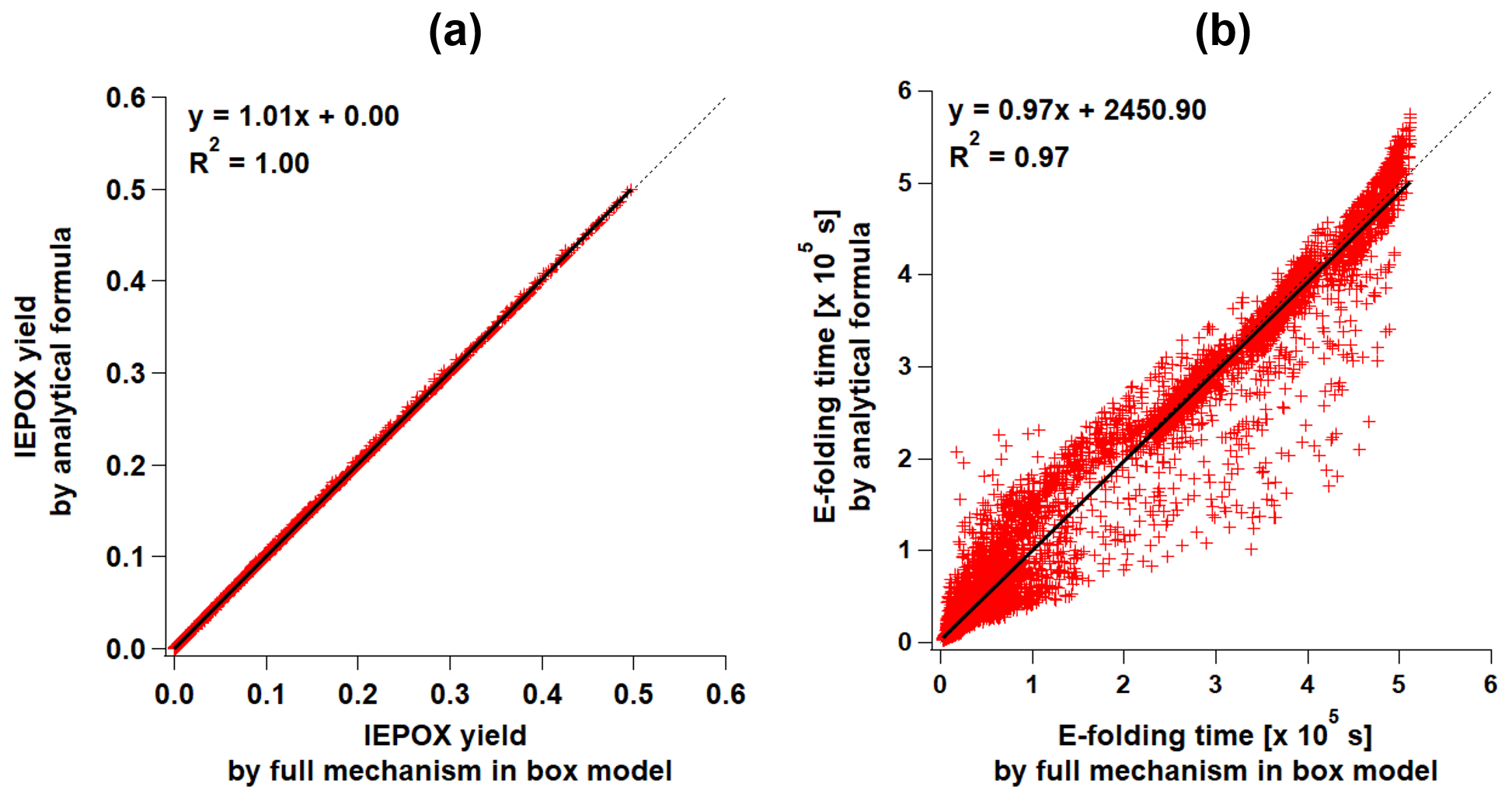
Figure 2 Scatterplots of the results of parameterizations (y axis) versus the full mechanism (x axis) box model results for (a) IEPOX molar yield (PAR2 and PAR3) and (b) formation timescale (PAR3). Formation timescale of the full mechanism box model was calculated as follows. We saved IEPOX concentrations for each time step. We defined the formation timescale as the time when the IEPOX concentration is closest to the $\mathrm{1}-\mathrm{1}/e$ (∼63 %) of the final IEPOX concentration.

Because IEPOX is formed immediately after isoprene emission in PAR2, it can result in an overestimated IEPOX concentration since the gas-phase chemistry has a limited rate. Therefore, we developed a third parameterization (PAR3) by modifying PAR2 by representing the formation timescale for IEPOX by adding a second intermediate:

$$\begin{array}{}\text{(15)}& \begin{array}{rl}& E_{\mathrm{Isoprene}}\times Y_{\mathrm{IEPOX}}\to {\mathrm{SOAP}}_I\stackrel{{\mathit{\tau }}_I}{⟶}\mathrm{IEPOX}\\ & \stackrel{f_{\mathrm{IEPOX}\to \text{IEPOX-SOA}}}{⟶}\text{IEPOX-SOA},\end{array}\end{array}$$

where τ_I is the formation timescale of IEPOX, which is calculated using the equation below.

$$\begin{array}{}\text{(16)}& \begin{array}{rl}& {\mathit{\tau }}_I=C_{\mathrm{0}}+C_{\mathrm{1}}\times {\displaystyle \frac{L_{\mathrm{ISOP}}^{C_{\mathrm{2}}}}{L_{\mathrm{ISOP}}^{C_{\mathrm{2}}}+C_{\mathrm{3}}^{C_{\mathrm{2}}}}}\\ & +C_{\mathrm{4}}\times {\displaystyle \frac{L_{\mathrm{ISOPOOH}}^{C_{\mathrm{5}}}}{L_{\mathrm{ISOPOOH}}^{C_{\mathrm{5}}}+C_{\mathrm{6}}^{C_{\mathrm{5}}}}}\times F\\ & +C_{\mathrm{7}}\times {\displaystyle \frac{L_{\mathrm{ISOPN}}^{C_{\mathrm{8}}}}{L_{\mathrm{ISOPN}}^{C_{\mathrm{8}}}+C_{\mathrm{9}}^{C_{\mathrm{8}}}}}\times \left(\mathrm{1}-F\right)\end{array}\end{array}$$

The functional form of Eq. (16) is the same as Eq. (12a) but excludes the last term (IEPOX loss). F is calculated using Eq. (12b) but with different constant values, which are provided in Table S3. Similar to the evaluation of PAR1, Y_IEPOX and τ_I were generally well predicted compared to 14 000 box model simulations (Fig. 2).

Three parameterizations from Eqs. (10), (13), and (15) were implemented in GEOS-Chem and evaluated in the rest of the paper. For brevity, hereinafter the parameterizations using Eqs. (10), (13), and (15) are referred to simply as PAR1, PAR2, and PAR3, respectively.

4 Results

4.1 Full chemistry vs. parameterizations

Figure 3 shows global annual surface maps of simulated IEPOX-SOA concentrations by using the full chemistry and the five parameterizations, while Fig. 4 compares the concentrations and burdens. The fixed 3 % yield parameterization (FIXED) underestimated IEPOX-SOA concentrations with a slope of 0.66. Similar to the 3 % parameterization, isoprene SOA concentrations with the VBS were substantially lower than those with the full chemistry and parameterizations. Isoprene SOA ratios of the VBS to the full chemistry were less than 20 % except for the aerosol source regions (Fig. 3c), because more semivolatile products can exist in aerosol phase due to high preexisting aerosol concentrations in the source regions. Furthermore, the VBS/full chemistry ratios were even higher than 1 for anthropogenic-source-dominant regions (California, western Europe, and Asia), where NO concentrations are high. However, the VBS predicted very low isoprene SOA concentrations in remote regions, leading to a low global burden (Fig. 4c). This dramatic difference came from the fact that the IEPOX-SOA is nonvolatile in the full chemistry, but the isoprene SOA is treated as semivolatile using the partitioning theory in the VBS. The VBS simulated most of the semivolatile products as gas phase (tropospheric burden of 232 Gg) rather than aerosol phase (tropospheric burden of 48 Gg), especially for remote regions where preexisting aerosol concentrations were low.

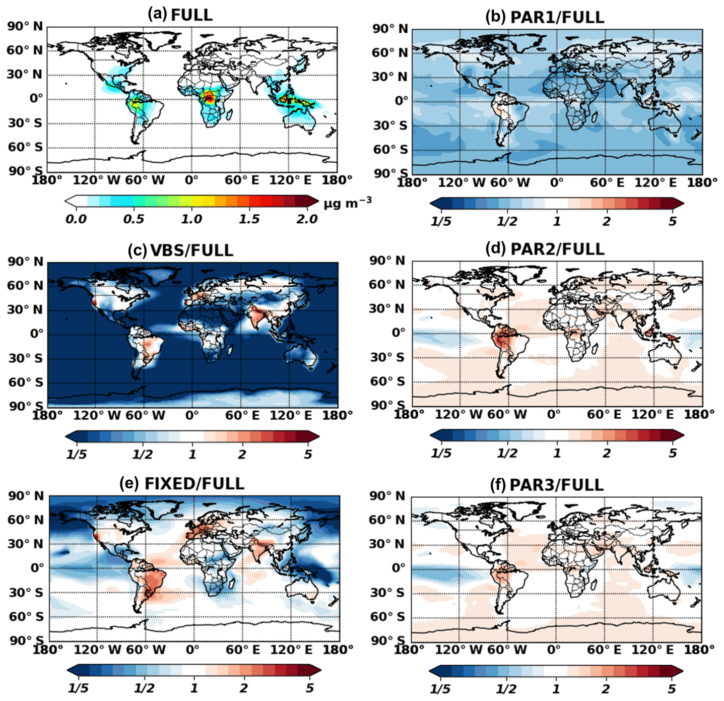
Figure 3 Annual mean (July 2013–June 2014) surface concentrations for IEPOX-SOA as predicted by full chemistry (a). Ratios of parameterized IEPOX-SOA concentrations to the full chemistry case are shown in panels (b)–(f).

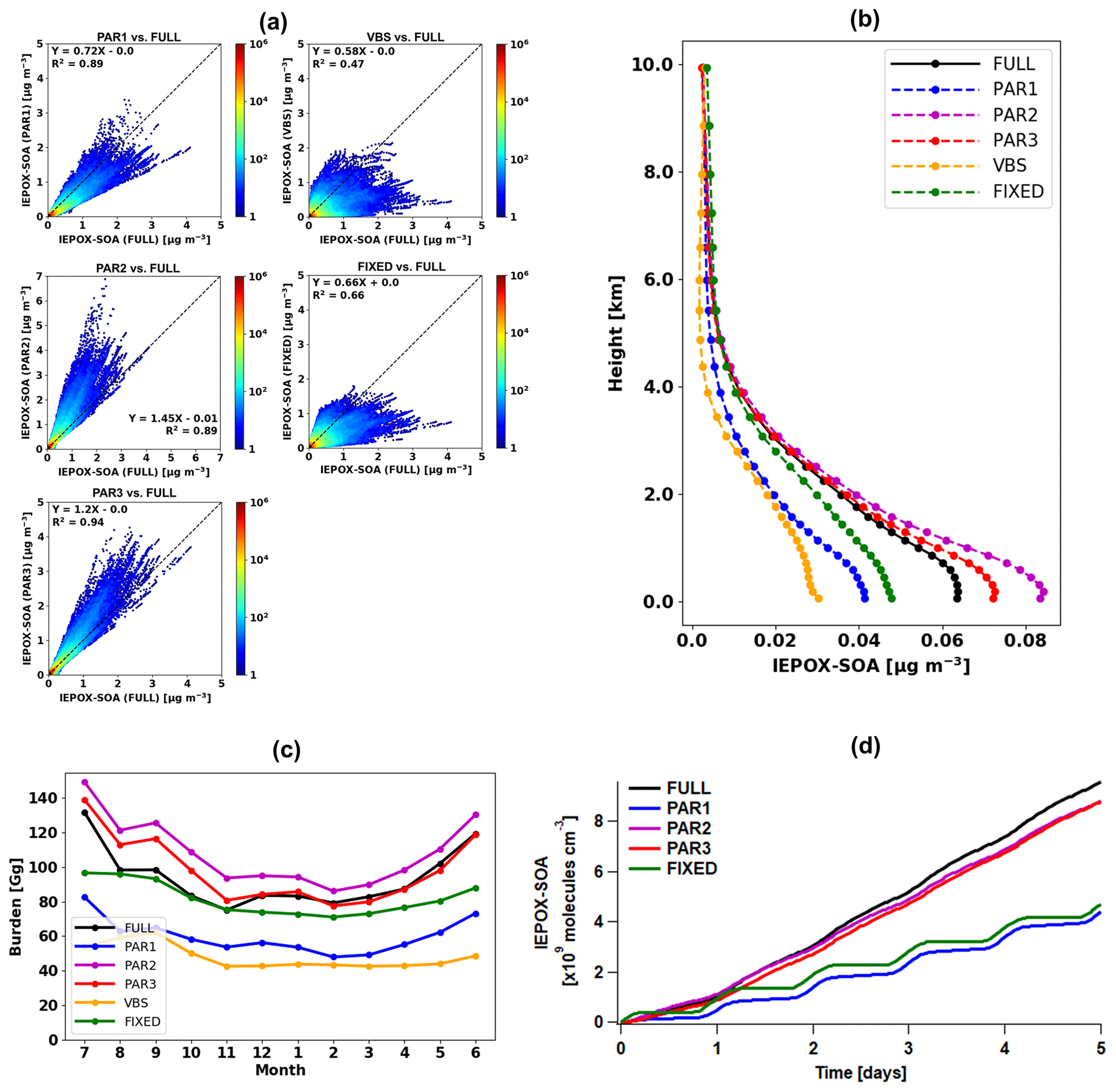
Figure 4 (a) Scatterplots of parameterized (y axis) versus full chemistry IEPOX-SOA (x axis) concentrations within the troposphere for July 2013–June 2014. Each point represents monthly averaged model grid value of IEPOX-SOA concentration. Colors represent the density of points, where densities were calculated by dividing x- and y-axis ranges into 100 by 100 grid cells. (b) Vertical profiles of global annual mean average IEPOX-SOA concentrations. The vertical locations of the markers indicate the midlevels of the vertical grid boxes in GEOS-Chem. (c) Time series of global tropospheric burdens of IEPOX-SOA (Gg). (d) Time series of IEPOX-SOA concentrations simulated by the box model. The VBS was not calculated with the box model, as it requires additional partitioning calculation with preexisting aerosols, which are calculated online in GEOS-Chem. Input chemical/meteorological fields were averaged from GEOS-Chem results for four major isoprene source regions (the southeastern United States: 30–40^∘ N, 100–80^∘ W; the Amazon: 10–0^∘ S, 70–60^∘ W; Central Africa: 5–15^∘ N, 10–30^∘ E; Borneo: 5^∘ S–5^∘ N, 105–120^∘ E). Input values represent annual mean values, which were calculated by using the first 2 d of each month model outputs at 30 min interval averaged within the PBL.

PAR1 generally underestimated IEPOX-SOA concentrations compared to the full chemistry simulation (slope = 0.72; R²=0.89), although with less bias and better skill than the default VBS (slope = 0.58; R²=0.47). An important driver of the low bias vs. the full chemistry was the diurnal variation of the chemical fields. Y_IEPOX-SOA is calculated in PAR1 using the instantaneous chemical fields at the time of isoprene emission, while in the full chemistry simulation (and in the real atmosphere) some processes proceed at different rates due to the different diurnal variations of key parameters.

To directly investigate the effect from the diurnal variation of the chemical fields, we used the box model to exclude other factors such as transport and deposition processes. First, we extracted isoprene emissions and chemical/meteorological fields affecting the IEPOX-SOA formation pathway from GEOS-Chem with 30 min temporal resolution (equivalent to the chemistry time step of GEOS-Chem used in this study). Then we averaged global chemical/meteorological fields within the PBL based on local time at each grid point for four major isoprene source regions (the southeastern United States, the Amazon, Central Africa, and Borneo). In this way, we constructed the source-region-averaged diurnal profile of chemical species, temperature, boundary layer height, isoprene emission, and reaction rate constants as inputs of the box model. The underestimation of IEPOX-SOA concentrations by PAR1 also occurred when we calculated IEPOX-SOA with the box model (Fig. 4d). This was caused by the diurnal variation of chemical/meteorological fields, as PAR1 successfully captured the time series of IEPOX-SOA when we used constant input values (Fig. S7).

The box model simulation with the source-region-averaged diurnal cycle resulted in similar IEPOX-SOA concentrations between the two parameterizations directly calculating IEPOX (PAR2 and PAR3) and the full chemistry (Fig. 4d). PAR2 and PAR3 also showed similar global spatial patterns vs. the full chemistry, but they slightly overestimated IEPOX-SOA over source regions (the Amazon, Central Africa, and Southeast Asia) (Fig. 3d and f), which is discussed in detail below.

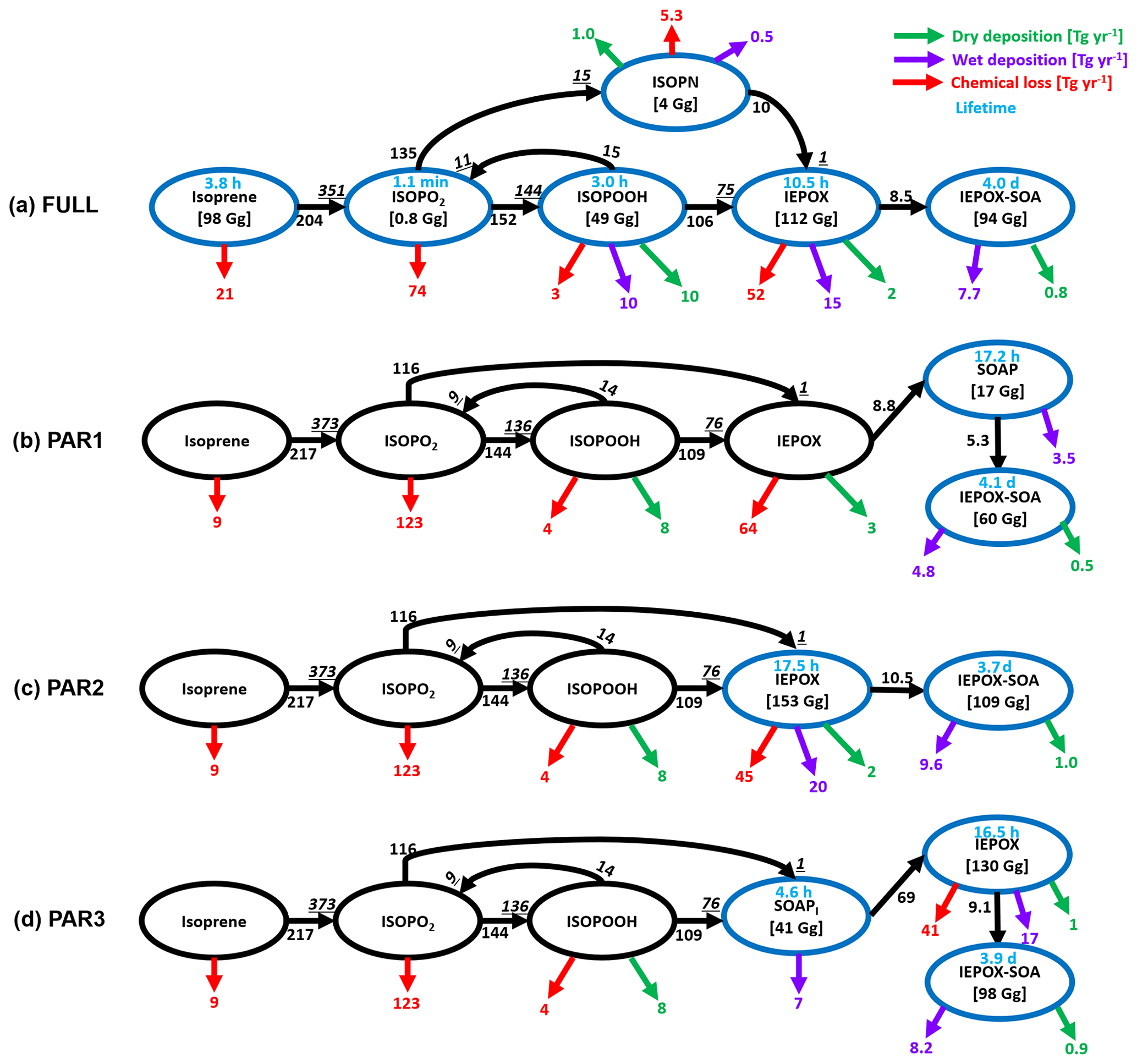
Figure 5 Global budget analysis of IEPOX-SOA formation from isoprene on a total annual mean basis (July 2013–June 2014). Black arrows with numbers show the IEPOX-SOA formation pathways. Two numbers are shown if the loss amount of reactant differs from the production amount of product (underline italic), which are caused by the different molecular weights and product yields. The isoprene nitrate (ISOPN) production pathway from isoprene + NO₃ reaction is not shown. Chemical losses that are not leading to IEPOX-SOA formation are shown in red arrows. Dry and wet deposition amounts are presented in green and purple arrows, respectively. Tropospheric burdens are given in brackets if species is explicitly simulated in the model. Blue circles are used for species that are explicitly simulated in each case.

The different performance between PAR1 and PAR2–3 was mainly caused by the differing influence of the diurnal variation profiles of chemical fields (Fig. S8). Furthermore, the diurnal variation effect influenced the IEPOX-SOA yield differently for each IEPOX-SOA precursor. Compared to the chemical pathways simulated by the full chemistry, PAR1 calculated higher chemical losses for isoprene but lower chemical losses for ISOPO₂ as revealed in global budget analysis (Fig. 5).

The underestimation of PAR1 was mainly caused by two reactions – IEPOX + OH and IEPOX reactive uptake. During the daytime when OH concentration was high, IEPOX + OH reaction became dominant, which reduced the IEPOX-SOA yield by PAR1. However, in the full chemistry model, IEPOX was less consumed by OH because IEPOX was not formed immediately from isoprene emissions. IEPOX peaked around 16:00 (all times are in local time; Fig. S8). Therefore, PAR1 overestimated the loss of IEPOX because it used a higher IEPOX loss rate compared to the full chemistry. In a similar way, PAR1 underestimated the IEPOX reactive uptake. In the full chemistry model, isoprene emission and OH peaked around local noon, but the IEPOX uptake rate constant peaked around 16:00 (Fig. S8). The IEPOX-SOA yield calculated at the time of isoprene emission (in PAR1) underestimated the real IEPOX-SOA yield. For example, the instantaneous IEPOX-SOA yield using both the isoprene emission and IEPOX reactive uptake rate constant at noon is lower than the yield calculated using the isoprene emission rate at 12:00 and the IEPOX reactive uptake rate constant at 16:00, when each process peaks.

Contrary to PAR1, which calculated IEPOX-SOA yield at the time of isoprene emission, PAR2 and PAR3 did not show a global underestimation because they only calculated IEPOX yield at the time of isoprene emission and then simulated the IEPOX reactive uptake explicitly. However, they showed slight overestimations over isoprene source regions such as the Amazon. We found that PAR2 and PAR3 generally overestimate the IEPOX-SOA when OH concentrations are low (Fig. S9), and the Amazon is one of low-OH regions from the GEOS-Chem model (Fig. S10). We attributed this tendency to the effects of lifetime of IEPOX precursor gases, for which OH concentrations are one of the major controlling factors. IEPOX yields in PAR2 and PAR3 are calculated using the instantaneous chemical fields. Therefore, the discrepancies between the explicit chemistry and PAR2–3 are reduced when the lifetimes of precursor gases are short. For the southeastern US where PAR3 did not show an overestimation, the lifetimes of isoprene and ISOPOOH were 0.9 and 1.5 h, respectively. The discrepancies are much larger for the Amazon: the lifetimes of isoprene and ISOPOOH are 12.3 and 6.1 h, respectively, due to low OH concentrations. As a result, PAR1–3 calculated the similar IEPOX production rate (1.9 Tg yr⁻¹) from the ISOPOOH + OH reaction compared to the full chemistry (1.8 Tg yr⁻¹) for the southeastern US, but the disagreement was larger for the Amazon (4.8 Tg yr⁻¹ in PAR1–3 vs. 3.9 Tg yr⁻¹ in the full chemistry). We anticipate that the discrepancy in source regions will be reduced in the future version of GEOS-Chem, because GEOS-Chem with the most-up-to-date isoprene mechanism predicts higher OH concentrations (up to 250 % increase) in the Amazon, central Africa, and Borneo regions compared to the isoprene mechanism used in this study (Fig. S17 in Bates and Jacob, 2019).

Table 1 Computational time estimation for the simulation of IEPOX-SOA using the full chemistry and parameterization cases in the box model and GEOS-Chem. The box model results are mean values of 1000 simulations based on 5 d integration time. The VBS was not simulated in the box model, because the VBS requires the partitioning calculation with preexisting aerosol concentrations, which are not available in the box model and are calculated online in GEOS-Chem. For GEOS-Chem, values were based on 7 d simulation using 32 cores on the NCAR Cheyenne machine. The Gprof performance analysis tool was used to calculate how much time was spent in subroutines with Intel Fortran Compiler 17.0.1 with the “-p” option. For GEOS-Chem, values were estimated by multiplying the total time spent in each process by the contribution of related reactions/species for each case, except for time estimates for chemistry of PAR1–3 and FIXED. For example, transport time in full chemistry was calculated by multiplying 2978 s (total transport time in Table S4) by 10 (total number of the explicit full chemistry species relevant to IEPOX-SOA formation)/173 (total number of advected species).

Parameterizations using chemical fields (PAR1–3) captured the variability of IEPOX-SOA well with R² values of 0.89–0.94. PAR3 always showed the best R² and slopes in terms of not only annual mean (Fig. 4a) but also monthly mean evaluation (Fig. S11), due to the fact that the structure of PAR3 was closer to that of full chemistry compared to other parameterizations. PAR3 requires three tracers and has a slightly higher computational cost than PAR1 and PAR2, which need two tracers to simulate IEPOX-SOA (Table 1).

In terms of vertical profiles (Fig. 4b), PAR2 and PAR3 again showed the best results, although these parameterizations slightly overestimated surface concentrations. On the other hand, PAR1, the VBS, and the 3 % yield substantially underestimated concentrations below 4 km.

The annual mean global tropospheric burden of IEPOX-SOA by full chemistry was 94 Gg vs. 60, 108, 98, 48, and 82 Gg for PAR1, PAR2, PAR3, the VBS, and the 3 %, respectively. The global IEPOX-SOA burden of PAR3 was within ∼5 % of the IEPOX-SOA burden simulated by full chemistry. Furthermore, we found that PAR2 and PAR3 showed similar monthly variations to the full chemistry (Fig. 4c). It also applied to the seasonal patterns of the hemispheric burden when we separated them for the northern and southern hemispheres as shown in Fig. S12. We also found that the fixed 3 % yield generally well reproduced the global burden amount of IEPOX-SOA, which gave some confidence in using the 3 % yield derived from the southeastern US summer conditions in terms of reproducing the global burden of IEPOX-SOA.

We calculated the annual mean global budgets of IEPOX-SOA simulated by the full chemistry and the parameterizations developed in this study (Fig. 5). Generally, each term is of the same order, with some differences in some cases, which are mainly due to the diurnal variation of the chemical fields. For example, the isoprene loss by O₃ and NO₃ was 21 Tg yr⁻¹ for the full chemistry, but this loss was reduced to 9 Tg yr⁻¹ in our parameterizations. Because NO₃ concentration was very low during the daytime when isoprene was emitted (Fig. S8), our parameterizations using the instantaneous yield applied to isoprene emission underestimated isoprene loss by NO₃. On the other hand, ISOPO₂ loss was higher in our parameterizations (123 Tg yr⁻¹) than in the full chemistry (74 Tg yr⁻¹) because chemical species affecting ISOPO₂ loss (CH₃CO₃ in Fig. S8) had similar diurnal variation patterns compared to the isoprene emission.

Although there were some differences between the results of the parameterizations and the full chemistry above, the parameterizations generally showed similar source and sink values compared to the full chemistry. The full chemistry showed annual production of 144 Tg yr⁻¹ ISOPOOH, which was similar to the value estimated by the parameterizations (136 Tg yr⁻¹). That was also the case for the annual production of IEPOX (75 Tg yr⁻¹ vs. 76 Tg yr⁻¹). Results in Fig. 5 imply that chemical-reaction-based parameterizations can capture global budgets of IEPOX-SOA chemistry with reasonable accuracy without explicit calculation of all intermediates. Furthermore, we found that the flux from IEPOX (or SOAP) to IEPOX-SOA was important for IEPOX-SOA simulation capability. For example, the flux from IEPOX to IEPOX-SOA in PAR3 was 9.1 Tg yr⁻¹, which was similar to the flux (8.5 Tg yr⁻¹) in the full chemistry, and PAR3 showed the best results. On the other hand, the production of IEPOX-SOA was 5.3 Tg yr⁻¹ in PAR1, which was the main reason for the IEPOX-SOA underestimation in that case.

When the explicit full chemistry changed, and the resulting IEPOX-SOA burden was increased by a factor of 2, our parameterizations showed very similar statistical parameters and evaluation results compared to the full chemistry (see Figs. 3 and 4 in the discussion paper and response to reviewers for more details). In other words, our parameterizations are robust to the changes in chemistry. This characteristic can be further confirmed by emission sensitivity tests as discussed below.

We investigated the effects of anthropogenic emission reductions on the simulated IEPOX-SOA concentrations. We conducted additional sensitivity tests for 2 months by reducing NO_x and SO₂ emissions by 50 %. New parameterizations (PAR1–3) showed similar sensitivities to the full chemistry case, but the VBS and fixed 3 % parameterizations did not reproduce changes relative to emission reductions (Fig. 6). Isoprene SOA concentrations by the fixed 3 % parameterizations remain the same because they are using the constant yield.

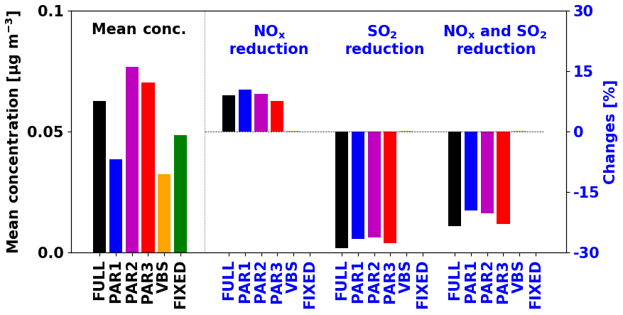
Figure 6 Global PBL averaged IEPOX-SOA concentrations (left, black) and the concentration changes with anthropogenic emission reductions (right, blue) for July–August 2013. The anthropogenic emissions were decreased by 50 % for each sensitivity case.

The VBS showed negligible sensitivities (less than 0.3 %). For the VBS, the change in the rate of oxidation of isoprene is the most important factor that can affect the isoprene SOA change. We found that OH concentrations were decreased in the NO_x reduction case (Fig. S13a). However, isoprene concentrations were increased (Fig. S13b) due to the reduced oxidant fields affecting isoprene loss (OH, O₃, and NO₃), because the chemical loss is the only pathway for isoprene loss (i.e., no isoprene is lost by dry and wet deposition) and isoprene emissions are unaffected. As a result, the initial rate oxidation of isoprene (rate constant × [isoprene] × [OH]) did not show the significant changes (Fig. S13d), as is also observed for isoprene SOA (Fig. S13f).

However, in the explicit full chemistry, for the sensitivity case of NO_x emission reduction, the contribution of HO₂ pathway was increased compared to the NO pathway, making more IEPOX and IEPOX-SOA. The reduced sulfate aerosol caused by the SO₂ emission reduction increases aerosol pH and decreases available aerosol surface area, which eventually decreases IEPOX reactive uptake. New parameterizations successfully captured these tendencies, indicating that they will be much more accurate compared to the current parameterizations in simulating the response of isoprene SOA to different scenarios, such as the response to future climates or anthropogenic emission reduction scenarios.

4.2 Computational time estimation

We estimated the computational time related to IEPOX-SOA simulation for the full chemistry and the different parameterizations. The box model was used for estimating the time needed for chemistry calculation using chemical reactions and dry depositions in Table S1. All the parameterizations showed much faster integration time compared to the full chemistry.

For estimation within GEOS-Chem, we used the Gprof function profiling program and categorized the results according to four major processes (chemistry, transport, dry deposition, and wet deposition), as shown in Table 1. One of the main advantages of using a function profiling program is that all of the timings are estimated at once without the need for multiple simulations. Because model computational time varies between individual executions even for the same machine and code (Philip et al., 2016), and because we examined a minority (IEPOX-SOA chemistry) of total GEOS-Chem model reactions, computational time estimation using multiple runs can lead to significant errors.

Our parameterizations (PAR1–3) reduced the computational time by factors of ∼5 and ∼2 compared to the full chemistry and the VBS, respectively. There was a factor-of-2 difference among parameterizations due to two main reasons. First, the difference between PAR1 and PAR2 arose from the additional calculation of formation timescale in PAR1 (Eq. 12). Second, the number of species was a key factor making the difference between PAR1 (two species) and PAR3 (three species). The 3 % showed the best efficiency – the cost of the 3 % case was ∼2–3 times less than those of PAR1–3, given its simplest structure.

When using GEOS-Chem, the full chemistry can still be chosen if the computational cost is not important or the detailed gas-phase chemical reactions are needed. Our developed parameterizations (PAR1–3) can be useful for researchers who are not interested in the details of isoprene SOA but who still want to have realistic aerosol concentrations in their simulations. PAR3 adds significant accuracy compared to the 3 % yield GEOS-Chem default for limited additional cost. The default VBS in GEOS-Chem v11-02-rc requires more computational cost than all of the parameterizations while being less accurate, and we recommend against its use in future simulations. Although we have used GEOS-Chem as a convenient development platform, the parameterizations may be especially useful for climate models for long-term simulations using other codes.

5 Conclusions

IEPOX-SOA is thought to dominate the contribution of isoprene to SOA, but it is formed by complex multiphase chemistry which cannot be accurately simulated by the commonly used lumped volatility-basis-set or fixed-yield SOA schemes. A detailed isoprene chemistry mechanism has been recently developed and implemented in some models, and recent studies have found good agreement between observed and simulated IEPOX-SOA concentrations. However, the detailed chemistry requires higher computational cost than the lumped SOA schemes, which may not be applicable for long-term multiscenario simulations in climate and similar models. The likely addition of other explicit SOA mechanisms as knowledge improves in the future would exacerbate this problem.

Here we developed parameterization methods to enable accurate yet fast IEPOX-SOA formation for climate model applications that mostly require having the correct SOA mass, spatiotemporal distribution, and response to changes in important precursors, for accurate calculations of the aerosol radiative effects. First, we developed a method to calculate the yield of IEPOX-SOA from isoprene emissions based on an approximate analytical solution of the full mechanism. Numerical fitting to box model results was introduced when the reaction could not be directly implemented for yield calculation. Formation timescales of key products were also used to more accurately represent the characteristic time of formation of IEPOX-SOA. Therefore, our parameterizations used two (PAR1 and PAR2) or three tracers (PAR3) to simulate IEPOX-SOA without the full chemical mechanism.

The parameterizations (especially PAR3) generally captured the spatial and temporal variations of IEPOX-SOA including sources, sinks, burdens, surface concentrations, and vertical profiles. Furthermore, the parameterizations showed better performance and lower computational cost compared to the current fixed-yield or VBS schemes in GEOS-Chem. Therefore, these parameterizations can be used for more accurate predictions of surface concentrations, as well as climate effects such as direct radiative forcing calculation.

The parameterizations can be easily updated if new values of key parameters are adopted by the community (e.g., Henry's law constant of IEPOX). The differences between the parameterizations and the full chemistry were mostly explained by nonlinear effects due to the diurnal variation of chemical/meteorological fields, which cannot be captured without additional complexity. One caveat is that some climate models use monthly mean fields of VOCs and oxidants. Because the diurnal variation was found to be important for accurate predictions of IEPOX-SOA, this may reduce the accuracy of the results for such models. We recommend that climate models account for diurnal variations for each chemical field in order to obtain more accurate IEPOX-SOA concentrations.

Detailed mechanistic studies in the laboratory, often aided by new mass spectrometry instrumentation with higher molecular detail, are leading to the development of many detailed SOA mechanisms, which will challenge global and especially climate models with their increased computational cost. The method developed in this study can be used to simplify other SOA mechanisms, allowing more accurate SOA simulations while limiting computational cost.