Estimating surface carbon fluxes based on a local ensemble transform Kalman filter with a short assimilation window and a long observation window: an observing system simulation experiment test in GEOS-Chem 10.1

We developed a carbon data assimilation system to estimate surface carbon fluxes using the local ensemble transform Kalman filter (LETKF) and atmospheric transport model GEOS-Chem driven by the MERRA-1 reanalysis of the meteorological field based on the Goddard Earth Observing System model, version 5 (GEOS-5). This assimilation system is inspired by the method of Kang et al. (2011, 2012), who estimated the surface carbon fluxes in an observing system simulation experiment (OSSE) as evolving parameters in the assimilation of the atmospheric CO₂, using a short assimilation window of 6 h. They included the assimilation of the standard meteorological variables, so that the ensemble provided a measure of the uncertainty in the CO₂ transport. After introducing new techniques such as “variable localization”, and increased observation weights near the surface, they obtained accurate surface carbon fluxes at grid-point resolution. We developed a new version of the local ensemble transform Kalman filter related to the “running-in-place” (RIP) method used to accelerate the spin-up of ensemble Kalman filter (EnKF) data assimilation (Kalnay and Yang, 2010; Wang et al., 2013; Yang et al., 2012). Like RIP, the new assimilation system uses the “no cost smoothing” algorithm for the LETKF (Kalnay et al., 2007b), which allows shifting the Kalman filter solution forward or backward within an assimilation window at no cost. In the new scheme a long “observation window” (e.g., 7 d or longer) is used to create a LETKF ensemble at 7 d. Then, the RIP smoother is used to obtain an accurate final analysis at 1 d. This new approach has the advantage of being based on a short assimilation window, which makes it more accurate, and of having been exposed to the future 7 d observations, which improves the analysis and accelerates the spin-up. The assimilation and observation windows are then shifted forward by 1 d, and the process is repeated. This reduces significantly the analysis error, suggesting that the newly developed assimilation method can be used with other Earth system models, especially in order to make greater use of observations in conjunction with models.

1 Introduction

The exchange of carbon among the atmosphere, land, and ocean contributes to changes in the Earth's climate and is also sensitive to climate conditions. The CO₂ concentration in the atmosphere is affected by both the natural variability of the Earth's planetary system and anthropogenic emissions. The terrestrial and oceanic ecosystems absorb more than one-half of anthropogenic CO₂ emissions (Le Quéré et al., 2016). One major scientific question is whether this rate of removal of CO₂ from atmosphere will continue in future and if it can be enhanced. It is thus essential to better quantify the dynamics of Earth surface carbon fluxes (SCFs) and the variations in carbon sources and sinks and their associated uncertainties.

A common approach for estimating SCF from atmospheric CO₂ measurements and atmospheric transport models is referred to as a “top-down” approach. The top-down methods estimate SCF through techniques such as Bayesian synthesis approach (Rödenbeck et al., 2003; Gurney et al., 2004; Enting, 2002; Bousquet et al., 1999), different types of ensemble Kalman filters (EnKF) (e.g., Peters et al., 2005, 2007; Feng et al., 2009; Zupanski et al., 2007; Lokupitiya et al., 2008), or variational data assimilation methods (e.g., Baker et al., 2006, 2010; Chevallier et al., 2009).

Kang et al. (2011, 2012) developed a top-down carbon data assimilation system by coupling an atmospheric general circulation model (AGCM), including atmospheric CO₂ concentrations, with the local ensemble transform Kalman filter (LETKF) (Hunt et al., 2007). The meteorological variables (wind, temperature, humidity, surface pressure) and CO₂ concentrations were assimilated simultaneously in order to account for the uncertainties of the meteorological field and their impact on the transport of atmospheric CO₂. They carried out observing system simulation experiments (OSSEs), and their carbon assimilation system achieved an accurate estimation of the evolving SCF at the model grid resolution for the first time, without requiring any a priori information. The surface carbon fluxes were considered “unobserved evolving parameters” by augmenting the state vector at each column with a surface carbon flux (SCF). The local ensemble transform Kalman filter (LETKF) then estimated this evolving parameter from the error covariance between the low-level atmospheric CO₂ and the estimated SCF, and, after a spin-up of about 1 month, the LETKF accurately recovered the “nature” run seasonal surface carbon fluxes.

Kang et al. (2011, 2012) used a short 6 h assimilation window for both atmospheric and CO₂ observations because atmospheric observations are usually assimilated at this frequency and because most ensemble Kalman filter methods require short windows to ensure that the forecast perturbation growth remains linear. Such a short data assimilation window, required by the LETKF, also protects the system from becoming ill conditioned (Enting, 2002, Fig. 1.3), and as a result it does not require additional a priori information. We note further that the use of such a short assimilation window differs very much from most other top-down approaches for estimating SCFs that use long assimilation windows varying from a few weeks to months or even years (e.g., Baker et al., 2006, 2010; Peters et al., 2005, 2007; Michalak, 2008; Feng et al., 2009; Liu et al., 2016).

Although the Kang et al. (2011, 2012) methodology was successful, it is computationally expensive, requiring ensemble forecasts and data assimilation, not only for the carbon variables but also for the standard atmospheric variables, in order to estimate the uncertainties of the CO₂ atmospheric transport process. In this study, we used an improved version of LETKF data assimilation system with a state-of-the-art atmospheric transport model, the GEOS-Chem (Bey et al., 2001; Nassar et al., 2013), which is driven by the MERRA-1 reanalysis of the Goddard Earth Observing System model, version 5 (GEOS5). The improved data assimilation system, unlike Kang et al. (2011, 2012), does not include an estimation of transport uncertainties related to the meteorological field.

The ultimate goal of our LETKF_C system is to estimate the grid-point SCFs, which, as in Kang et al. (2011, 2012), are treated as time-evolving parameters in the system. As mentioned before, an ensemble Kalman filter requires a short assimilation window in order to have the ensemble perturbations evolve linearly and remain Gaussian. On the other hand, it is well known that the training needed to estimate evolving parameters through data assimilation could be quite long, thus it benefits from having many observations. Therefore, a short assimilation window would shorten the training period needed for the estimation of the SCF error covariance, and therefore lengthen the spin-up time.

To address this problem, we developed a new version of the LETKF using the running-in-place (RIP) method to accelerate the spin-up of EnKF data assimilation (Kalnay and Yang, 2010; Wang et al., 2013; Yang et al., 2012). Like RIP, the new assimilation system uses the “no cost smoothing” algorithm (Kalnay et al., 2007b) that allows shifting at a negligible cost the Kalman filter solution forward or backward within a given assimilation window. Briefly, the new scheme works as follows: a long “observation window” (e.g., 7 d, containing all the observations within 7 d) is used to create a temporary LETKF ensemble analysis at 7 d. Then the RIP smoother is used to obtain a final analysis at 1 d. This analysis has the advantage of being based on a short assimilation window, which makes it more accurate, and of having been exposed to the 7 d of observations, which accelerates the spin-up time. The assimilation and observation windows are then shifted forward by 1 d, and the process is repeated. We have tested this new method (short assimilation, long observation window), achieving a significant reduction of analysis errors, and we believe that this method could be useful in other data assimilation problems.

This paper is organized as follows: Sect. 2 briefly describes the new system used for CO₂ data assimilation (LETKF_C). Section 3 explores the effect of combining assimilation and observation windows in an OSSE framework. Section 4 presents results of the proposed methodology applied to CO₂ data. A summary and discussion are presented in Sect. 5.

2 LETKF_C data assimilation system

A data assimilation system includes a forecast model, observations, and a data assimilation method that optimally combines them. In the proposed LETKF_C data assimilation system we use the GEOS-Chem as the forecast model and LETKF as the data assimilation method. The pseudo-observations for our OSSE experiments are created at the locations of the real carbon observations from Orbiting Carbon Observatory-2 (OCO-2) satellite (Crisp et al., 2004).

2.1 GEOS-Chem model and the “nature” run

GEOS-Chem is a global 3-D atmospheric chemical transport model driven by the NASA reanalysis (MERRA-1) meteorological fields from the Goddard Earth Observing System data assimilation, version 5, by the NASA Global Modeling and Assimilation Office (Bosilovich et al., 2015). This model has been applied worldwide to a wide range of atmospheric composition and transport studies. The GEOS-Chem model used in this study is the version 10.01 with a resolution of 4^∘ × 5^∘ (latitude × longitude) and 47 hybrid pressure–sigma vertical levels for CO₂ simulation (Nassar et al., 2013). GEOS-Chem is driven by the MERRA-1 reanalysis with 72 hybrid vertical levels, extending from the surface up to 0.01 hPa. The data used in this study was provided by the GEOS-Chem support team, based at the Harvard and Dalhousie Universities with support from the NASA Earth Science Division and the Canadian National and Engineering Research Council, who re-gridded the original data of spatial resolution of 0.25^∘ × 0.3125^∘ into the resolution of 4^∘ × 5^∘.

GEOS-Chem requires the SCFs as a set of parameters at each grid point in order to simulate the CO₂ concentration in the atmosphere. It is not possible to observe the global SCFs directly. Therefore, the SCFs are created from a “bottom-up” approach (considered “truth” in our experiments) and used for the simulation of atmospheric CO₂ concentration with GEOS-Chem. The bottom-up SCFs used in this study include the three components shown in Eq. (1): (1) terrestrial carbon fluxes (F_TA), (2) air–sea carbon fluxes (F_OA), and (3) anthropogenic fossil fuel emissions (F_fe).

$$\begin{array}{}\text{(1)}& \mathrm{SCF}=F_{\mathrm{TA}}+F_{\mathrm{OA}}+F_{\mathrm{fe}}\end{array}$$

The F_TA values are derived from the VEgetation Global Atmosphere Soils (VEGAS) model (Zeng et al., 2004, 2005), forced by the real evolving weather, obtained from the GEOS-Chem. The F_OA values are from Takahashi et al. (2002), a climatological seasonal cycle estimated for the 1990s, and the F_fe values are from the Fossil Fuel Data Assimilation System (FFDAS) for the year 2012 (Asefi-Najafabady et al., 2014). The air–sea carbon flux and F_fe values were scaled using the global carbon budget data of Le Quéré et al. (2015) in order to include interannual variations. A nature run for atmospheric CO₂ concentration simulation is driven by the SCFs in units of (kgC (m² yr)⁻¹) based on all three datasets.

In OSSEs, the nature run serves as the truth. We assume that the true bottom-up carbon fluxes are not known in our data assimilation experiments, and they will be estimated using the atmospheric pseudo-observations derived from the truth, as described in more detail below. The nature run obtained by coupling GEOS-Chem with VEGAS is fairly realistic (figure not shown), so we use it to create the pseudo-OCO-2 observations for the period of January 2015–March 2016.

2.2 Pseudo-observations

The ultimate goal of this model–data assimilation system is to estimate the SCFs at every grid point using real observations such as the conventional surface CO₂ measurements of GlobalViewplus (GV+) flask network provided by Cooperative Global Atmospheric Data Integration Project (2016) and the observations from satellites such as the Greenhouse Gases Observing Satellite (GOSAT) (Yokota et al., 2004), and the Orbiting Carbon Observatory-2 (OCO-2) (Crisp et al., 2004). Therefore, it is very beneficial to choose a realistic observation network to generate the pseudo-observations for testing the proposed data assimilation system. In this study, we developed the pseudo-observations for the OSSE assimilation experiments, based on a realistic OCO-2 observation product.

The OCO-2 observations are the CO₂ column-averaged dry air mole fractions over the entire OCO-2 pixel (defined as XCO₂). The synthetic observations cover the entire globe once every 14 d with very high spatial resolution. This includes 24 samples per second along the satellite track within ∼7 km span. The observations are expected to be highly correlated over a short length scale. Furthermore, the observation quality is greatly affected by conditions such as cloud cover, surface type, and the solar zenith angle at the time of measurement. The OCO-2 retrieval algorithm uses a warning level (WL) between 0 and 19 to indicate the quality of measurements, where WL = 0 means “most likely good”, and WL = 19 means “least likely good” observations. To avoid highly correlated measurements being treated as independent measurements and to bring the spatial resolution in line with the resolution of atmosphere transfer model, David Baker provided an OCO-2 observation dataset which averaged the synthetic XCO₂ in 10 s time window using the “good-quality” observations retrieval defined by $\mathrm{WL}<=\mathrm{15}$ (David Baker, personal communication, April 2017).

The OCO-2 retrievals used to obtain averages are based on the NASA Atmospheric CO₂ Observations from Space XCO₂ retrieval Algorithm version 7r (O'Dell et al., 2012), as archived at https://disc.gsfc.nasa.gov/datasets/OCO2_L2_Lite_FP_7r/summary (last access: 23 March 2017). A two-step averaging method has been used in order to avoid the final average being disproportionately weighted to one part of the averaging bin (track) with more good-quality retrievals. In the first step, the “good-quality” retrievals, defined as $\mathrm{WL}<=\mathrm{15}$ and XCO₂_quality_flag = 0 (another quality indicator of the data), are averaged over 1 s bins, with weights inversely proportional to the square of each retrieval's posterior uncertainty. In the second step, all the 1 s bins with at least one valid retrieval are averaged over a 10 s interval to create 10 s averaged data. The OCO-2 averaging kernels are similarly averaged to create 10 s mean averaging kernels. This averaging method had been used for similar purposes in the recent study by Basu et al. (2018). In this study, we further aggregated the observations from David Baker at the nearest GEOS-Chem output time of 00:00, 06:00, 12:00, and 18:00 UTC for each model day. The typical 1 d coverage of observation of OCO-2 is shown in Fig. 1. The values of XCO₂ in the winter are significantly larger than those in summer of the Northern Hemisphere and the OCO-2 observations are missing in the winter for midlatitude and high-latitude regions (latitude > ∼30). We used the actual location, timescales, and error scales of the OCO-2 observations to create the pseudo-observations for our experiment. The pseudo-observations are created by obtaining the true CO₂ from the nature run using the location and time of the valid observation, then adding random errors with due consideration to the scales of the corresponding real observations. These derived pseudo-observations used in this study are based on the real observations associated error scales; thus, they are much more realistic than the GOSAT observations also used in Kang et al. (2012) because they are anchored on the real OCO-2 observations, their quality, and their statistical representation.

Figure 1 The 10 s average of good-quality OCO-2 XCO₂ observations (warning level < = 15), obtained from David Baker for (a) 1 January 2015 and (b) 1 July 2015.

2.3 The LETKF data assimilation system

The ensemble Kalman filter (EnKF) is a powerful tool for data assimilation that was first introduced by Evensen (1994). The key attribute of this method is to derive the forecast uncertainties from an ensemble of integrated model simulations. A variety of ensemble Kalman filter assimilation methods have been proposed (Burgers et al., 1998; Houtekamer and Mitchell, 1998; Anderson, 2001, 2003; Bishop et al., 2001; Whitaker and Hamill, 2002; Tippett et al., 2003; Ott et al., 2004; Hunt et al., 2004). The local ensemble transform Kalman filter (LETKF) introduced by Hunt et al. (2007) is chosen for this study.

The LETKF is an extension of the local ensemble Kalman filter (Ott et al., 2004) with the implementation of the ensemble transform filter (Bishop et al., 2001; Wang and Bishop, 2003). It is widely used for data assimilation, including several operational centers, and was also used for carbon data assimilations by Kang et al. (2011, 2012).

As discussed earlier, we follow Kang et al. (2011) in estimating the SCFs as evolving parameters, augmenting the state vector C (the prognostic variable of atmospheric CO₂) with the parameter SCF, i.e., $X=[\mathrm{C},\mathrm{SCF}{]}^T$. The analysis mean ${\stackrel{\mathrm{‾}}{X}}^{\mathrm{a}}$ and its ensemble perturbations X^a are determined by Eq. (2.1, 2.2) at every grid point, and the ensemble analysis is used as the initial conditions for the ensemble forecast in the next cycle.

$$\begin{array}{}\text{(2)}& {\stackrel{\mathrm{‾}}{X}}^{\mathrm{a}}={\stackrel{\mathrm{‾}}{X}}^{\mathrm{b}}+X^{\mathrm{b}}\stackrel{\mathrm{̃}}{K}(y^{\mathrm{o}}-{\stackrel{\mathrm{‾}}{y}}^{\mathrm{b}})\end{array}$$

$$\begin{array}{}\text{(3)}& X^{\mathrm{a}}=X^{\mathrm{b}}\left[\right(K-\mathrm{1}){\stackrel{\mathrm{̃}}{P}}^{\mathrm{a}}{]}^{\mathrm{1}/\mathrm{2}}\end{array}$$

Here, ${\stackrel{\mathrm{‾}}{X}}^{\mathrm{b}}$ is the mean of the forecast (background) ensemble members; X^b is a matrix, whose columns are the background perturbations of $X_k^{\mathrm{b}}-{\stackrel{\mathrm{‾}}{X}}^{\mathrm{b}}$for each ensemble member $X_k^{\mathrm{b}}$ (k=1,..., K), where K is the ensemble size; y^o is a vector of all the observations; ${\stackrel{\mathrm{‾}}{y}}^{\mathrm{b}}$ is the background ensemble mean in observation space (${\stackrel{\mathrm{‾}}{y}}^{\mathrm{b}}=H\left({\stackrel{\mathrm{‾}}{X}}^{\mathrm{b}}\right))$, where H is the observation forward operator that transforms values in the model space to those in the observation space; ${\stackrel{\mathrm{̃}}{P}}^{\mathrm{a}}={\left[{\left(Y^{\mathrm{b}}\right)}^T{R}^{-\mathrm{1}}{Y}^{\mathrm{b}}+\frac{\left(K-\mathrm{1}\right)I}{r}\right]}^{-\mathrm{1}}$ is the analysis error covariance matrix in ensemble space, which is a function of Y^b=HX^b , the matrix of background ensemble perturbations in the observation space, R, the observation error covariance (e.g., measurement error, aggregation error, representativeness error), and of r, a multiplicative inflation parameter; and $\stackrel{\mathrm{̃}}{K}={\stackrel{\mathrm{̃}}{P}}^{\mathrm{a}}{Y}^{\mathrm{b}}{R}^{-\mathrm{1}}$. LETKF simultaneously assimilates all observations within a certain distance at each analysis grid point, which defines the localization scale. Hunt et al. (2004) introduced a four-dimensional version, and Hunt et al. (2007) provide a detailed documentation of the 4-D LETKF that we are using.

2.4 Choosing the long observation window (OW) and the short assimilation window (AW)

Like other data assimilation methods, LETKF proceeds in analysis cycles that consist of two steps, a forecast step and an analysis step. In the analysis step, the model forecast (also called prior or background) and the observations are optimally combined to produce the analysis (also called the posterior), which is the best estimate of the current state of the system under study. In the forecast step, the model is then advanced in time with the analysis as the initial condition and its result becomes the forecast for the next analysis cycle. All observations within the assimilation time window are used to constrain the state at the end of the assimilation window.

The focus of this study is on the estimation of SCFs that are time-varying parameters in GEOS-Chem. As mentioned earlier, a preliminary LETKF analysis, which provides the weights for each ensemble perturbation, is performed over a longer window (e.g., 7 d, with observations starting at time t). Then, the “no cost” smoothing (Kalnay et al., 2007b; Kalnay and Yang, 2010) is applied, using the same analysis weights obtained at the end of the long observation window (e.g., 7 d) for each ensemble member but combining the ensemble perturbations at the end of the corresponding short assimilation window (e.g., 1 d). This creates the final 1 d analysis (at time t+AW), which benefits from the information from all the observations made throughout the long OW (7 d) and from the linearity of the perturbations in the short AW of 1 d, which is required for accuracy. At this time the procedure is repeated starting at t+AW, which is 1 d later.

In this new approach, we have the flexibility to combine a short assimilation window (AW) of length m (e.g., m=1 d) with a long observation window (OW) of length n (e.g., n=7 d) to improve the estimation of SCF. In the forecast step, the model is integrated from t to t+n to produce the forecast corresponding to the observations within the OW. In the analysis step, the observations and corresponding forecasts within the OW are used by the LETKF to estimate optimal weights for the ensemble members. The no cost smoother applies these optimal weights to determine the analysis of the model state and the SCF parameter at t+m. The resulting analysis is then used as the initial conditions for the next analysis cycle starting from time t+m.

2.5 Experimental setup

In our experiments we used an ensemble size of 20 members, which was reasonable since the data assimilation only includes one state variable (CO₂ concentration) and one parameter variable (SCF). A similar experiment but with 80-member ensemble size showed only slight improvement of assimilation quality (figure not shown) but dramatically increased the computational cost. The initial ensemble is created by random selection of the state and flux values from the model-based nature run for both SCF and atmospheric CO₂ concentration. Therefore, the initial uncertainties of fluxes and CO₂ values are equivalent to their “natural” variability. Based on a sensitivity analysis, we found a horizontal localization radius of 15 000 km is optimal for our system. Following Kang el al. (2012), a vertical localization is also applied by assigning a larger weight to the CO₂-updating layers near the surface, to reflect the expected dominance of layers near the ground in the change of the total column CO₂ measured by OCO-2.

2.6 Additive inflation method

Inflation is very important for our LETKF_C data assimilation system. The LETKF uses the forecast ensemble spread to represent forecast uncertainties. All EnKFs tend to underestimate the uncertainty in their state estimate because of nonlinearities and the limited number of ensemble members (Whitaker and Hamill, 2002). Underestimating the uncertainty (ensemble spread) leads to overconfidence in the background state estimate and less confidence in the observations, which will eventually lead the EnKF to ignore the observations and result in filter divergence. This is also true for our carbon-LETKF data assimilation system. The ensemble spread of CO₂ in GEOS-Chem model decreases during model integration when the ensemble members are using the same meteorological forcing and SCF values, which is very different from the system with prognostic meteorological fields where the ensemble spread of model state increases during model integration (not shown). The ensemble spread of SCFs also does not increase during model integration because the SCFs are predicted using persistence, and the LETKF decreases the ensemble spreads for both SCFs and CO₂ during analysis steps. Therefore, without inflation, the ensemble spread of the CO₂ and SCFs would be continuously decreasing during data assimilation, and soon would become too small for LETKF to accept any observations, causing filter divergence.

There are different types of inflation methods that address the problem of overconfidence, such as multiplicative inflation, relaxation to prior, and additive inflation (e.g., Anderson and Anderson, 1999; Mitchell and Houtekamer, 2000; Zhang et al., 2004; Whitaker et al., 2008; Miyoshi, 2011). For this study, we chose additive inflation, which adds random fields to the analysis before the ensemble forecast of the next analysis cycle. Additive inflation has some advantages compared to multiplicative inflation because it prevents the effective ensemble dimension from collapsing toward the dominant directions of error growth (Whitaker et al., 2008; Kalnay et al., 2007a). We applied additive inflation to the ensemble of atmospheric CO₂ and SCF to increase perturbations in the initial conditions for the next time step. It is important for an additive inflation method to minimize the impact of model imbalance and initial shocks generated by adding the random fields into a model. Following Kang et al. (2012), the added fields are selected randomly from the model nature run. Pairs of atmospheric CO₂ and surface CO₂ flux fields are chosen randomly from the model nature run within 1 year before the analysis time; their ensemble mean is removed and their differences are scaled to a magnitude corresponding to 30 % of model seasonal variance to create the ensemble of random fields for additive inflation. Therefore, each selected random field is balanced, and when it is added into model, the balance will be essentially maintained.

3 Sensitivity analysis for AW and OW length

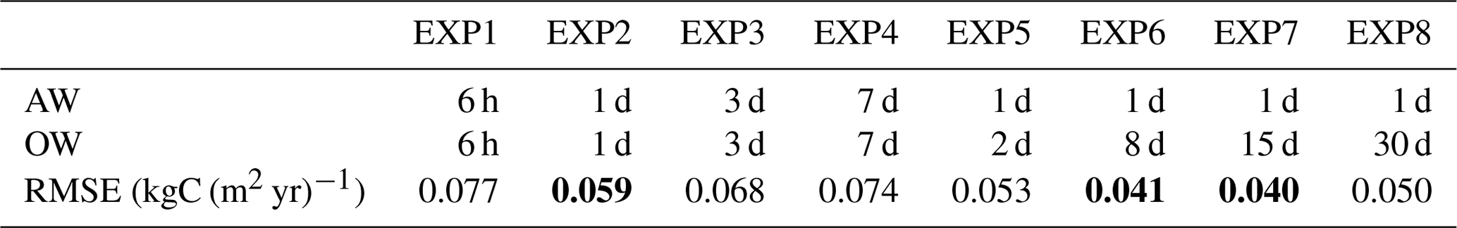
We tested the new version of the LETKF with short AW and long OW, described in previous sections by conducting two sets of experiments using the LETKF_C system in an OSSE framework with OCO-2-like observations. The first set of experiments used the regular 4-D LETKF settings (with a single window length AW = OW) to investigate the effect of the length of AW for estimating SCF. In the second set of experiments, we investigated the optimal OW length after choosing the best AW from the first set of experiments. The assimilation period for all experiments was 1 January 2015 to 1 March 2016. The annual mean RMSE differences are calculated from the simulation results by removing the spin-up period of the first 2 months (January and February 2015). The average period is from 1 March 2015 to the end of February 2016. The details of experimental settings are shown in Table 1.

Table 1 Lengths of assimilation windows (AWs) and observation window (OWs) and the resulting time-averaged global mean RMSEs for different experiments. The first four experiments use a regular 4-D LETKF, with AW = OW. The last four experiments use AW = 1 d, found to be optimal, and different OWs.

3.1 Sensitivity analysis for different assimilation windows

The sensitivity of SCF estimates to the length of AW was investigated based on the first set of experiments (EXP1–EXP4) with regular 4-D LETKF settings, where the length of OW is the same as that of the AW. All experiments used the same observations and initial conditions. Since the temporal coverage of the OCO-2 observation network is too sparse for our LETKF_C assimilation system to estimate the SCF signal over short timescales, we focus on evaluating the estimation of SCF for seasonal and longer timescales.

Figure 2 shows the estimated global total surface fluxes from the first set of experiments. The true global total surface fluxes show a clear seasonal cycle with very large carbon uptake during the growing season of the Northern Hemisphere (NH), from May to August, and carbon release during other seasons, with the peak release during November. All experiments reproduced the seasonal cycle of SCF fairly well.

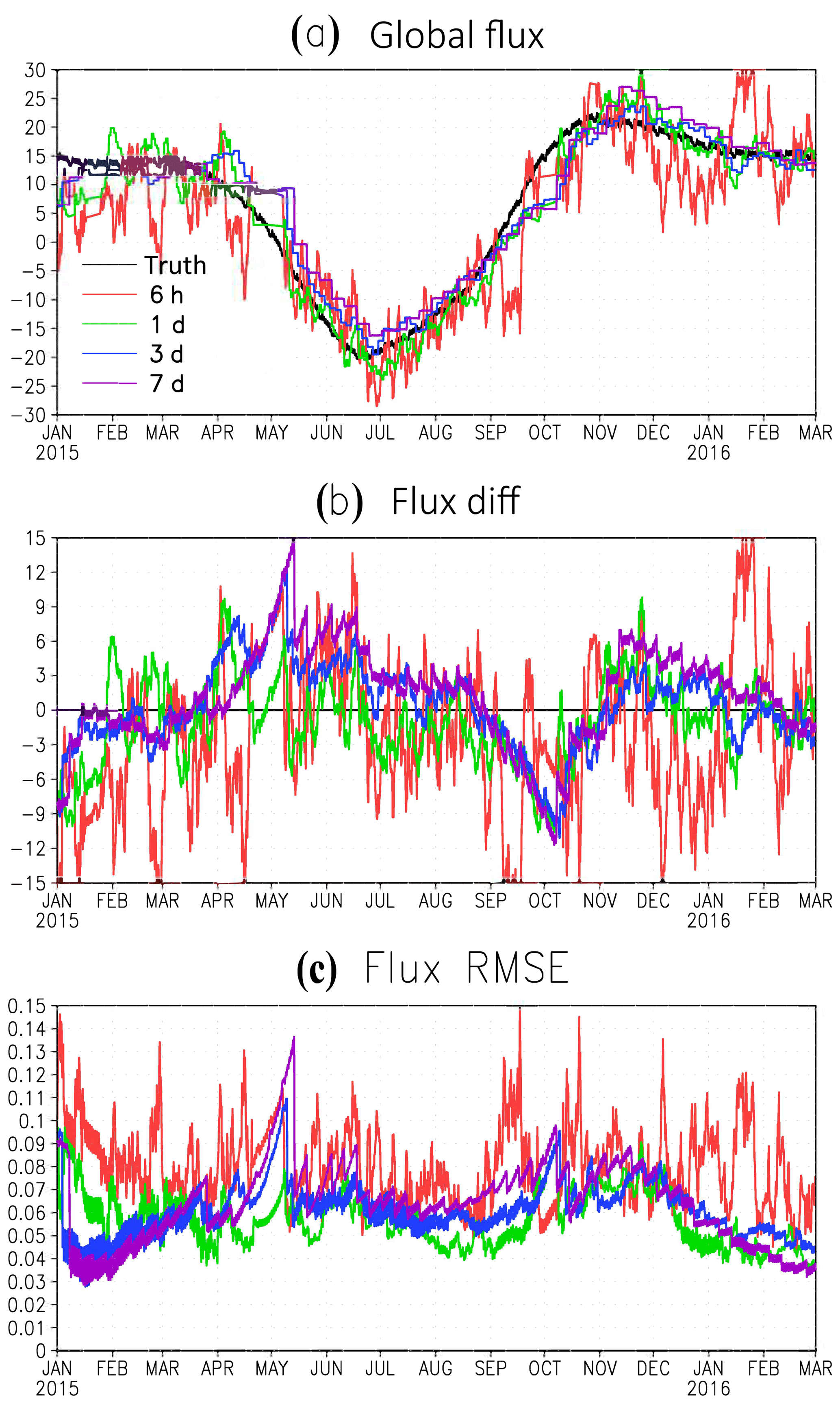
Figure 2 (a) The global total SCF from the nature run (“truth”, black line) and from the estimations of the first set of experiments with different AW. (b) The difference of global total SCF between the estimations from the experiments with different AW and the nature run (truth). (c) The global average RMSE of the estimated SCFs from the experiments with different AW.

When the AW is very short (6 h), there is large-magnitude and high-frequency noise overlaying the seasonal cycle. The magnitude of high-frequency errors of SCF estimation in EXP1 is comparable with the seasonal variability of SCF (Fig. 2a). When the AW = 7 d, the high-frequency errors of estimation decay but the long assimilation window increases the analysis RMSE (EXP4). The EXP2 with AW = 1 d produced the best estimation of SCF among all four experiments with equal observation and assimilation windows (Fig. 2).

The advantage of AW = 1 d (EXP2) is clearly seen from the smaller average global root-mean-square error (RMSE) (Fig. 2c). The RMSE of surface carbon flux is calculated as follows:

$$\begin{array}{}\text{(4)}& \mathrm{RMSE}\left(t\right)=\sqrt{E_x\left({\left(F^{\mathrm{a}}\left(x,t\right)-F^{\mathrm{n}}\left(x,t\right)\right)}^{\mathrm{2}}\right)},\end{array}$$

where x and t are space and time location; F^a and Fⁿ indicate the analysis and the true SCF from the nature run, respectively. E_x is spatial average. The estimations from experiments with long AW (3 and 7 d) have a smaller RMSE for the first 3 months (January to March), when the truth had very little variation because the long AWs enhance the signal and smooth the high-frequency noise. However, the experiments with long AW can miss the fine-scale signals of SCF variation and fail to catch its variations with time. As a result, the estimations with long AW showed large RMSE during the period when SCF had larger variations. The estimation with an AW of 6 h also showed very large RMSE because of the overwhelming high-frequency noise. Thus, the estimation with an AW of 1 d had the smallest RMSE among all of the experiments with a regular 4-D LETKF.

The time-averaged RMSEs of SCFs is calculated as follows:

$$\begin{array}{}\text{(5)}& \mathrm{RMSE}\left(x\right)=\sqrt{E_t\left({\left(F^{\mathrm{a}}\left(x,t\right)-F^{\mathrm{n}}\left(x,t\right)\right)}^{\mathrm{2}}\right)},\end{array}$$

which shows very similar spatial patterns but different amplitudes for different experiments (Fig. 3). The large RMSEs of SCF estimation located in the southeastern USA and the southeast of both China and Russia, resembled that of the SCF variance (not shown). The regions of higher variance indicate more information is needed to resolve such large variance by observations, which is hard to achieve. As expected, the SCF RMSE of 0.059 from EXP2 with an AW of 1 d is significantly smaller than the RMSE from EXP1 with a short AW of 6 h (0.077 kgC (m² yr)⁻¹) and EXP3 and EXP4 with longer AWs of 3 d (0.068kgC (m² yr)⁻¹) and 7 d (0.074 kgC (m² yr)⁻¹), respectively.

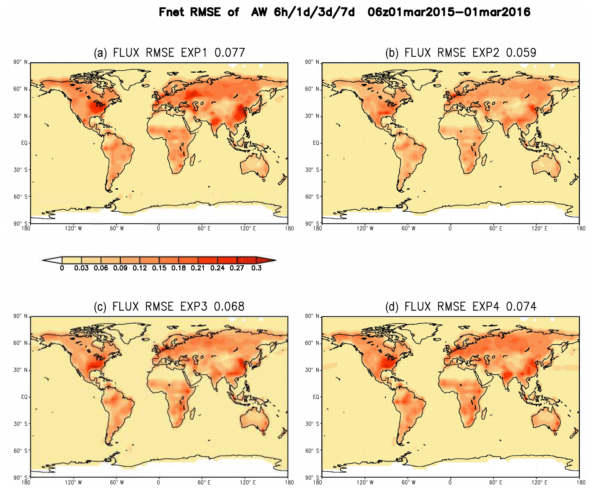
Figure 3 The spatial pattern of the annual mean RMSE of estimated SCF from the experiments with different AW (EXP1–4) for the average period from 1 March 2015 to the end of February 2016. (January and February 2015 are treated as a spin-up period for our experiments).

Our results suggest that the optimal AW for estimating SCF is about 1 d. This is distinctly different from previously published studies that indicate that either a very short AW (6 h) (Kang et al., 2011, 2012), or a very long AW (longer than a few weeks) is optimal (e.g., Baker et al., 2006, 2010; Peters et al., 2005, 2007; Michalak, 2008; Feng et al., 2009). A short AW can better constrain the model state and therefore produce a better parameter estimation. However, a very short AW of 6 h can degrade the SCF estimation with high-frequency noise in our LETKF-C system. We postulate that the high-frequency noise is related to the sampling errors in the CO₂–SCF covariance that has a smaller signal-to-noise ratio compared to those in experiments with longer AWs.

The same results can be obtained from the same experiments with different initial times, indicating the robustness of our findings (figure not shown). The convergence of estimated SCFs from the experiments starting from months with big SCF variation, such as April, is slightly slower than the experiments from the time with small SCF variation, such as January. While the estimated SCFs converge in a few analysis cycles (a few days) in our system (Fig. 2), the small difference of convergence rate does not make any significant impact on the quality of estimated SCFs. Moreover, the calculation of RMSE of estimated SCFs has excluded the spin-up period of the first 2 months to remove the potential impact of the initial conditions and initial time.

3.2 Sensitivity analysis for different observation windows (OW)

The results presented earlier and associated discussion suggest that parameter estimation through data assimilation benefits from a long training time and having a sufficient number of observations, implying that the length of OW is critical for the estimation of desired parameter(s). We investigated the effect of such sensitivity to find out the suitable length of OW for estimating SCF in the second set of experiments (EXP5–EXP8), all based on the optimum AW = 1 d that was identified from the first set of experiments but using different OW lengths.

The estimated global total SCFs in the second set of experiments show a clear seasonal cycle matching the truth (Fig. 4a). Compared with EXP2 (OW = 1), shown with the green line in Fig. 2a, EXP5 (OW = 2 d) reduced the high-frequency noise significantly when the OW length was increased from 1 to 2 d. There is still some high-frequency noise in the SCF estimation for EXP5 because the observations for 2 d are not sufficient to smooth out the high-frequency noise introduced into the estimation through data assimilation. The estimated global total SCFs for EXP6 (OW = 8 d), EXP7 (OW = 15), and EXP8 (OW = 30) are much smoother than that of EXP5 (OW = 1 d) because of their longer OW. However, the estimation for OW of 30 d shows a clear time-shift compared with the truth, especially during the transient period when the majority of ecosystems and plants are switching from dormant phase in the winter to the growing phase in the spring. The surface carbon fluxes change rapidly during this period. The time-shift can also be seen in the estimations for these experiments with an OW of 15 d, but it is less pronounced. In the proposed LETKF technique, most of observations in a long OW are introduced at a time later than the assimilation time. Since the SCFs are temporally evolving parameters, the information (variation) of future surface fluxes is brought into the estimation of current time when the future observations are included in the OW. Therefore, the estimated SCFs with a very long OW tend to shift towards its future value. The estimated SCFs with moderate OW = 8 and 15 d (EXP6 and EXP7) are more accurate than those with a short OW of 2 d (EXP5) and very long OW of 30 d (EXP8) by avoiding the significant high-frequency noise observed in EXP5 (OW = 2 d) and the significant time-shift present in EXP8, with a very long observation window (OW = 30 d). The global mean RMSEs of estimated SCF from OW = 8 and 15 d (EXP6 and EXP7) are significantly smaller than those from OW = 2 and 30 d, i.e., EXP5 and EXP8 (Fig. 4c).

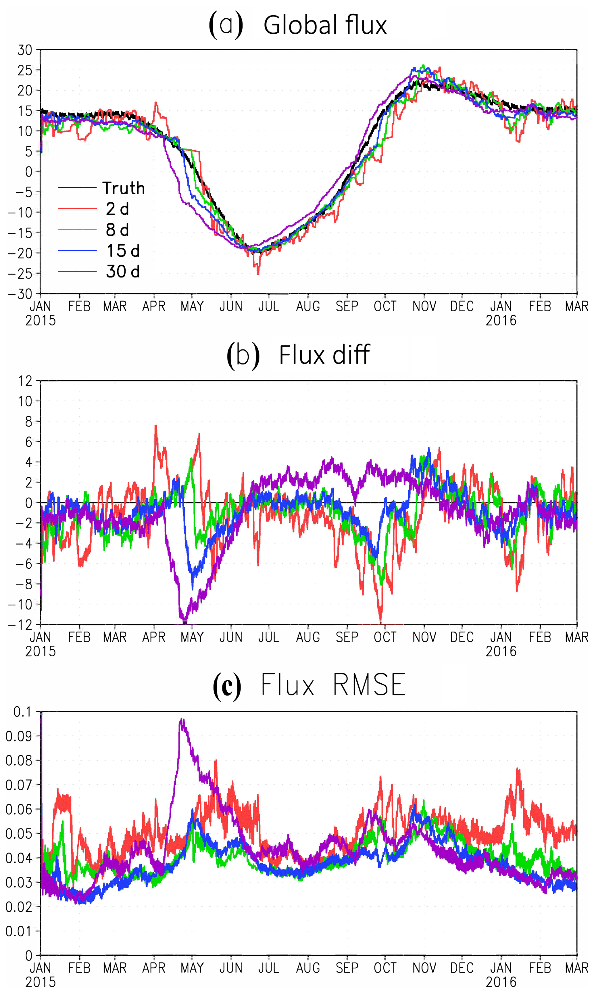
Figure 4 Same as Fig. 2, except for the second set of experiments with different OW but the same AW of 1 d.

The spatial pattern of time-averaged RMSE of SCF for EXP5 (OW = 2 d; Fig. 5) is similar to those in the first set of experiments, which had short AW = OW (Fig. 3). The regions with large RMSE in EXP5 (OW = 2 d) disappear with OW = 7 and 15 d in EXP6 and EXP7 because the long OWs enhance the signals for SFC estimation. The large RMSE in SCF estimates for EXP8 (OW = 30 d) are primarily in the Northern Hemisphere midlatitudes because of the time-shift in estimations with OW = 30 d. The mean RMSEs of experiments with moderate OWs of 8 and 15 d are 0.041 and 0.040kgC (m² yr)⁻¹, respectively, which is significantly smaller than those from experiments with OWs of 2 d (0.053 kgC (m² yr)⁻¹) and 30 d (0.050 kgC (m² yr)⁻¹).

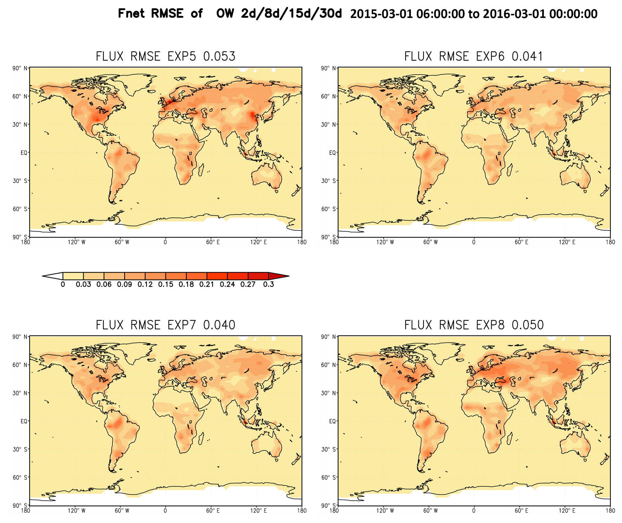
Figure 5 Same as Fig. 3, except for the second set of experiments with different OW but similar AW of 1 d.

However, a longer OW requires a longer forecast period for each forecast step, which results in additional computational time and cost. For example, EXP7 with an OW of 8 d used 8 times more computational time compared to EXP2. Furthermore, the length of the OW is also constrained by the timescale of estimation parameters. A long OW tends to generate a time-shift for its estimation. For seasonal and longer timescales, OW(s) in the moderate range of 8–15 d appear to be most suitable for the LETKF_C estimates of the SCF. EXP6 and EXP7 show almost the same quality of SCF estimation, but EXP6 has higher computational efficiency. The best configuration thus appears to be EXP6 with an OW of 8 d and AW of 1 d, referred as the “benchmark” experiment hereafter.

We note that the high-frequency noise in EXP1 with a short AW of 6 h can be smoothed out by a long OW (i.e., 8–15 d). We postulate that an experiment with an AW of 6 h and OW 8 d will produce similarly realistic estimations as the benchmark experiment; however, it would require much more computational time.

4 Evaluating estimated fluxes from the benchmark experiment

With the moderately long observation and short assimilation windows, we obtained best estimates of surface carbon fluxes, and their seasonal cycle. This section describes the SCF estimates from the benchmark experiment (AW = 1 d, OW = 8 d). Figure 6 shows a comparison of surface carbon fluxes based on the benchmark assimilation experiment and the nature (truth) run for Northern Hemisphere summer (June, July, and August) and winter seasons (December, January, and February). The bottom-up carbon fluxes used in the nature run show a very strong seasonal cycle over all of the continents except Antarctica. The Northern Hemisphere midlatitude areas are very large carbon sinks in the summer and carbon sources in the winter, as expected. The strong seasonal cycle of surface fluxes is mainly related to the variability of terrestrial ecosystems that absorb a large amount of CO₂ during the growing season (spring and summer) and release carbon back to the atmosphere during dormant seasons (fall and winter). The estimated surface fluxes in the seasonal timescale follow the truth closely. The benchmark assimilation experiment closely reproduces the spatial pattern of surface fluxes globally, for different seasons. The difference between the benchmark estimation and truth shown in Fig. 6e, f are very small. There are some positive carbon flux differences over Northern Hemisphere midlatitudes in the winter, thus a positive bias in estimated atmospheric CO₂ concentration is expected.

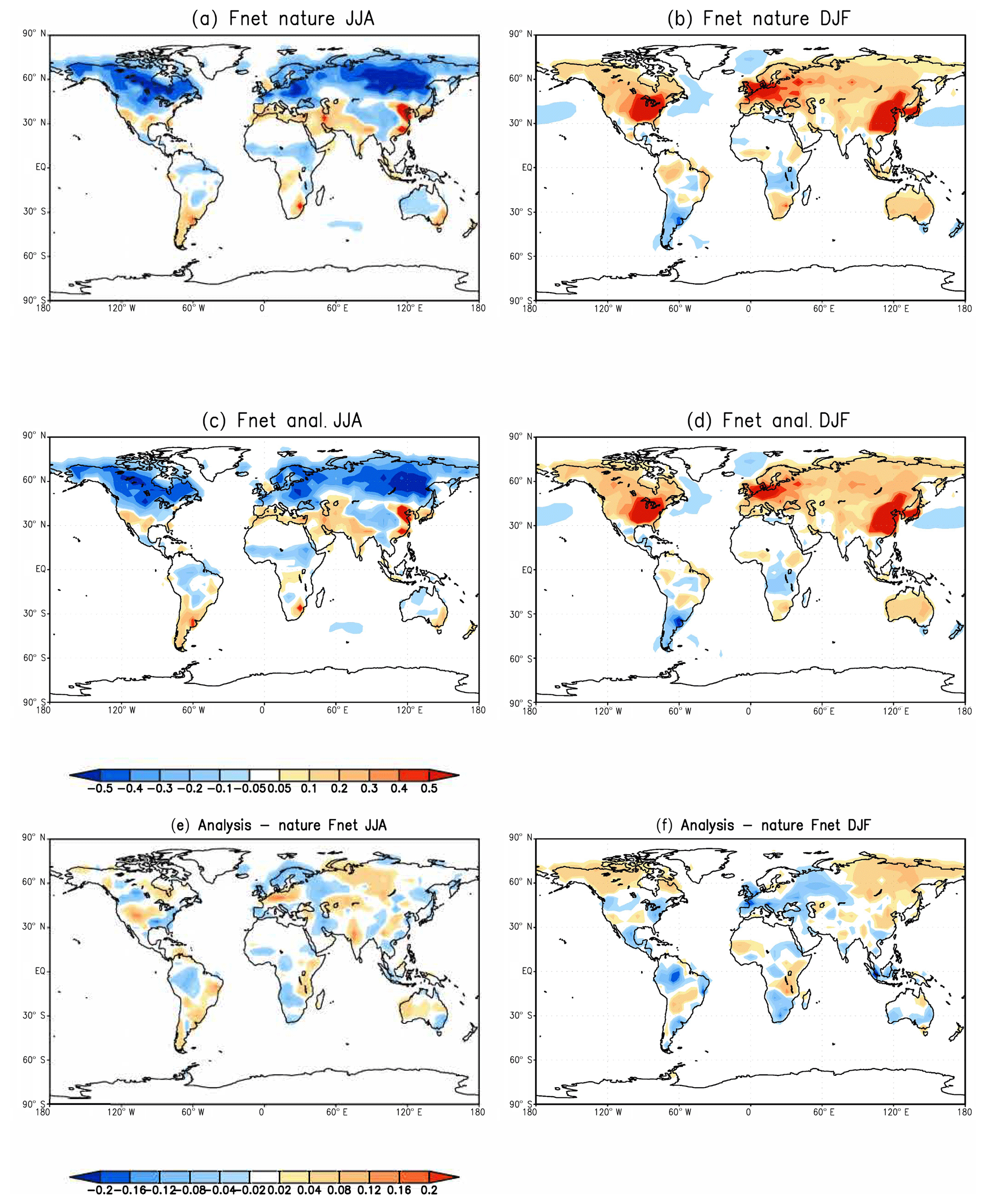
Figure 6 The SCF of the “nature” run and an estimation from the benchmark experiment (AW = 1 d, OW = 8 d) for Northern Hemisphere summer (a, c and e), and winter (b, d, and f). Panels (a) and (b) are the “truth” from the nature run, panels (c) and (d) are the estimates from benchmark experiment, and panels (e) and (f) are the difference between estimation and truth.

The analysis of CO₂ concentrations matches the nature run well. The error pattern also matches the CO₂ seasonal cycle and the error pattern of estimated SCF. Figure 7 shows the comparison of surface atmospheric CO₂ concentrations between the benchmark assimilation experiment and the nature (truth) run for the Northern Hemisphere summer and winter. The spatial pattern of assimilated CO₂ matches the truth very well. The analysis successfully reproduced the seasonal cycle of CO₂ over Northern Hemisphere midlatitudes, with low CO₂ concentration in summer (Fig. 7a–c) and high CO₂ in winter (Fig. 7b–d), consistent with the seasonal cycle of CO₂ absorption and release from terrestrial ecosystems. There are positive CO₂ concentrations located at high latitudes of the North American and East Asian regions during winter 2016 (Fig. 7f), due to the positive bias in estimated SCF (Fig. 6f).

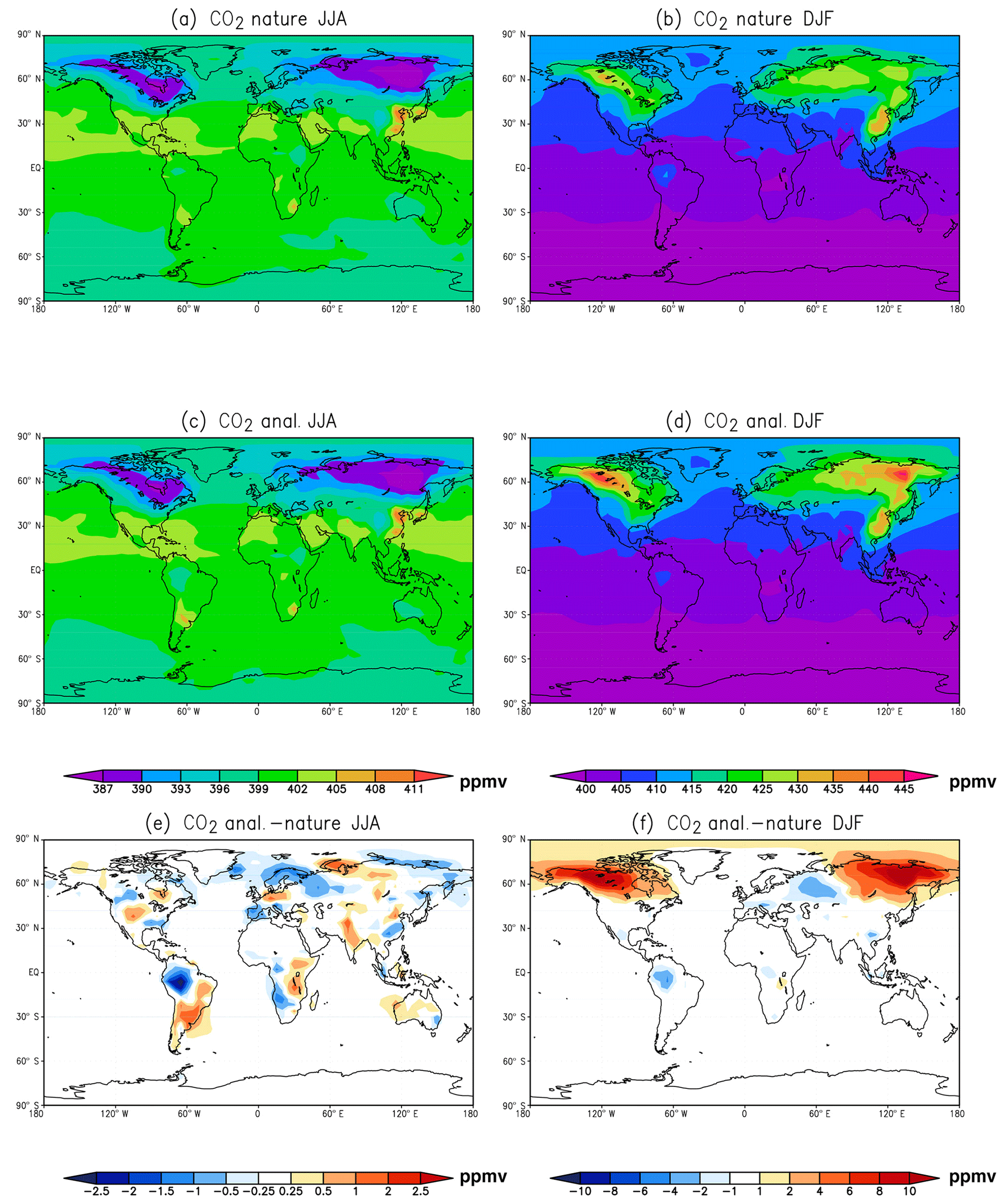
Figure 7 Same as Fig. 6, except for surface concentrations of CO₂. Where panels (a) and (c) share the upper left color bar; Panels (b) and (d) use the upper right color bar.

The consistency of annual mean estimated SCF for both benchmark experiment and truth is a very important feature for our LETKF_C assimilation system (Fig. 8a). In EnKF assimilation the ensemble spread is considered a good representation of uncertainties associated with both parameters and model state (e.g., Evensen, 2007; Liu et al., 2014). The surface carbon fluxes are special parameters that vary with time and it is very hard to quantify their uncertainty during assimilation. When the ensemble spread of parameters are too small to drive a model with a robust response, the estimation fails. The additive inflation with 30 % of nature variability is used to maintain the amplitude of parameter ensemble spread. Although the ensemble spread of the global total surface flux, in our experiments, is bigger than its error (Fig. 8a), we were still able to estimate the global total surface CO₂ fluxes (ensemble mean) and their seasonal variability very well. This is consistent with findings of Liu el al. (2014) that parameter estimation can tolerate some inconsistency between parameter ensemble spread and parameter error.

Figure 8 (a) The global total SCF of “truth” and estimation from the benchmark experiment: the black line is the truth, the green line is the ensemble mean of the estimation, and the yellow shading is the ensemble spread. (b) The global mean RMSE of the estimated SCF from the benchmark experiment(AW = 1 d, OW = 8 d).

The global mean RMSE of SCF decreases from an initial value of ∼0.1 to ∼0.04 kg C m⁻² yr⁻¹ in just a few analysis cycles (Fig. 8b). It does not further decrease during following assimilation cycles because the SCF values vary temporally. The signals added by observations are mainly used to reproduce the temporal variation in SCF.

It is very important for a SCF estimation to reproduce the spatial distribution of the annual mean of the SCF, since it identifies the carbon sources and sinks in the Earth system. Though the amplitude of annual mean SCF is much smaller than the seasonal cycle of SCF, the estimated spatial pattern of annual mean SCF in the benchmark experiment (Eq. 5) is generally consistent with the truth (Fig. 9).

$$\begin{array}{}\text{(6)}& \mathrm{\Delta }F\left(x\right)=E_t\left(F^{\mathrm{a}}\left(x,t\right)\right)-E_t\left(F^{\mathrm{n}}\left(x,t\right)\right)\end{array}$$

In summary, we found that the OSSE experiments using long observation windows and short assimilation windows resulted in the best estimates of SCF.

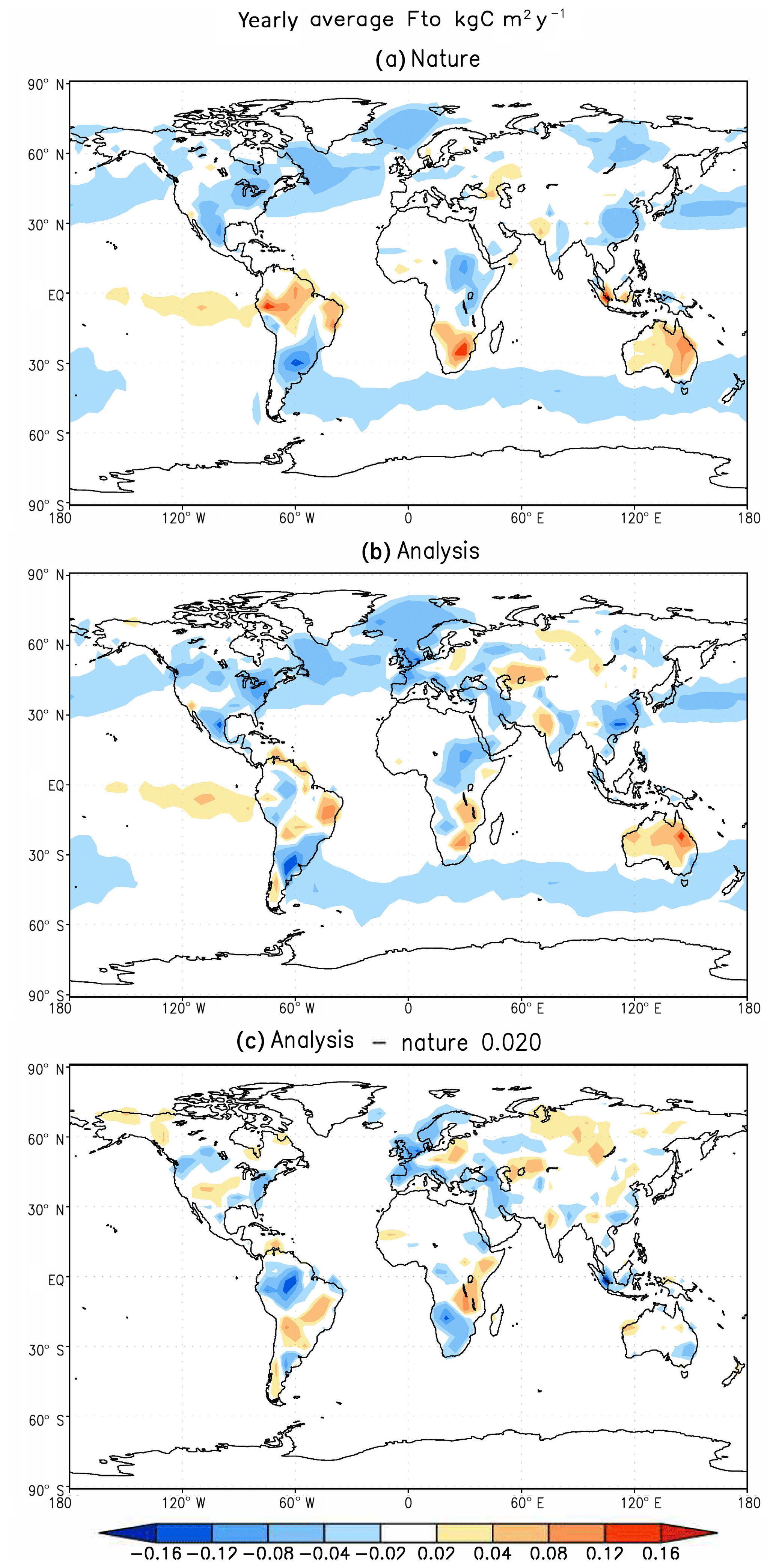
Figure 9 (a) The annual mean of SCF (with the F_fe removed) for the “nature” run, (b) the annual mean of estimated SCF (with the F_fe removed) from the benchmark experiment, and (c) their differences.

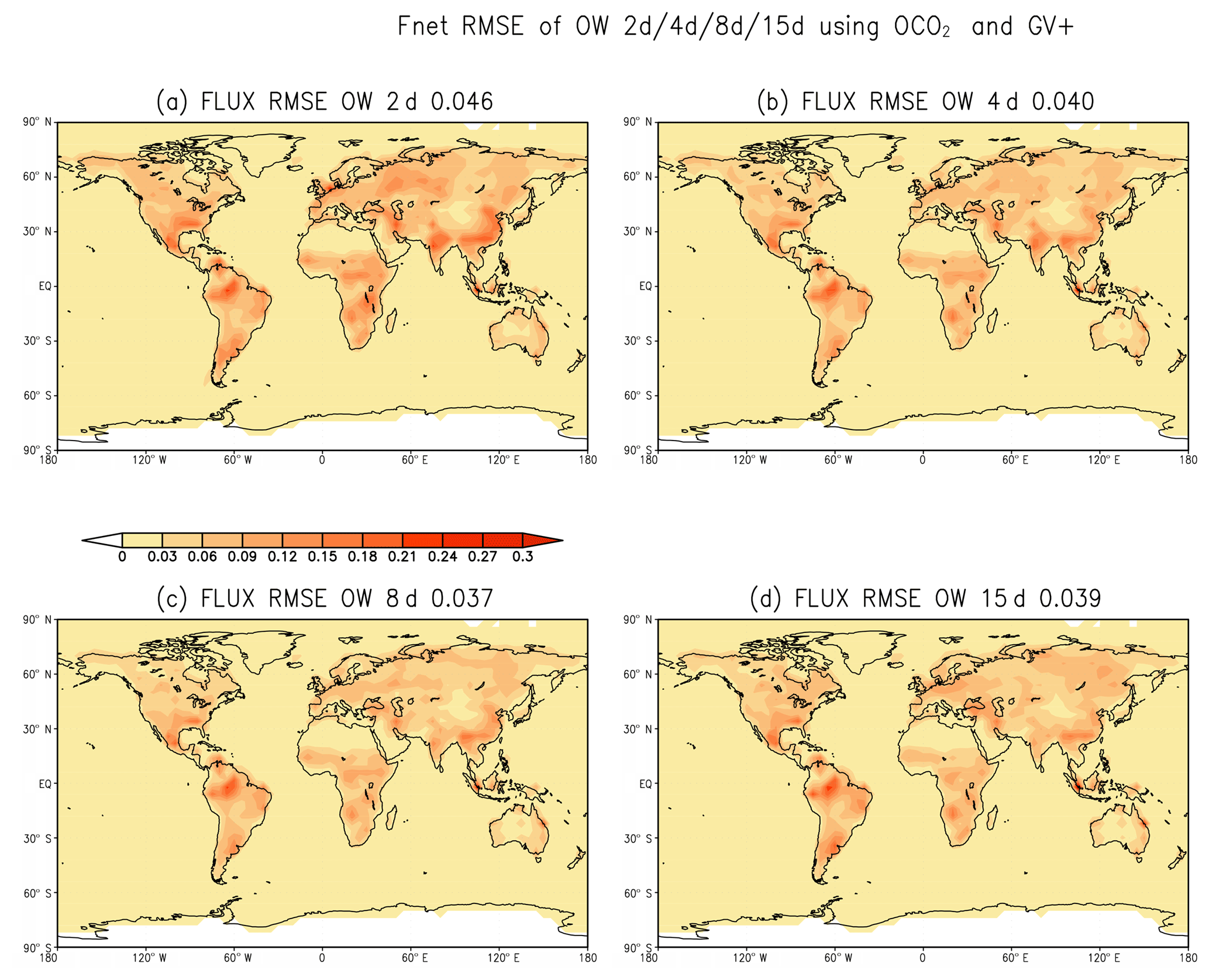
Figure 10 Same as Fig. 5, except for assimilating both OCO-2 and GV+ pseudo-observations. Panels (a), (b), (c), and (d) show the results with OWs of 2, 4, 8, and 15 d respectively.

5 Summary and discussion

We have developed a LETKF GEOS-Chem carbon data assimilation (LETKF_C) system for estimating the surface carbon fluxes (SCFs). The true GEOS-Chem atmospheric transport model is driven by the single realization of meteorology fields from MERRA reanalysis. The proposed data assimilation system captured the true SCF spatial and temporal variability well. The system performed best with a choice of short assimilation and long observation windows.

The LETKF requires a short assimilation window to avoid an ill-posed condition caused by the nonlinear processes in the forecast model with a long forecast time. The parameter estimation favors a long training period and many observations. Based on these features, we developed a new method to accurately estimate the SCF. The new scheme separates the original assimilation time window into observation (OW) and assimilation (AW) windows, allowing for the flexibility to apply an OW that is different to the AW. Like the running-in-place (RIP) method, the new technique takes advantage of the no cost smoothing algorithm developed for the LETKF by Kalnay et al. (2007b) that allows the transportation of the Kalman filter solution forward or backward within the observation window.

The new method was applied to the LETKF_C system in the OSSE mode using a dataset developed based on the OCO-2 observation characteristics. The sensitivity experiments for this model assimilation system demonstrated that the new technique, i.e., using a short AW and long OW, significantly improves the SCF estimation as compared to a regular 4-D LETKF with identical observation and assimilation windows. The best AW for SCF estimation is 1 d, which is different from the typical AW of 6 h used in the meteorological assimilations. An OW in the range of 8–15 d is required to estimate the surface carbon fluxes for seasonal and longer timescales. The benchmark experiment with an AW of 1 d and the OW of 8 d successfully reproduced the mean seasonal and annual SCF.

Our working hypothesis was that the optimal OW for the estimation of SCF could be reduced with more observations. We examined this hypothesis by using simulated OCO-2 observations and GlobalViewPlus (GV+) observations. Similar to the OCO-2 pseudo-observations, the GV+ pseudo-observations were also generated based on the actual location, time, and corresponding error scale of the GV+ flask observations. The results show that the AW and OW lengths of 1 d and 8 d, respectively, are also optimal using both the OCO-2 and GV+ observation characteristics. We estimated the SCF using the OCO-2 and GV+ pseudo-observations with the identical experiment settings as the OCO-2 experiments, except we replace the experiment with very long OW of 30 d with an experiment with a short OW of 4 d to better evaluate the impact from short OWs. Thus, the current experiments settings are using OW of 2, 4, 8, and15 d.

The results from these experiments show that the AW and OW lengths of 1 d and 8 d, respectively, are still optimal for both the OCO-2 and GV+ observation characteristics (Fig. 10). Generally, the time mean RMSE of estimated SCF with OCO-2 and GV+ (Fig. 10) are smaller than the corresponding estimates for OCO-2 only (Fig. 5). The short OW of 2 d performs worse than the moderate OWs of 4, 8, and 15 d. The time-averaged global mean RMSE is 0.046 kgC (m² yr)⁻¹ for experiments with an OW of 2 d (Fig. 10a). The time-averaged global mean RMSE is only 0.040, 0.037, and 0.039 kgC (m² yr)⁻¹ for experiments with OWs of 4, 8, and 30 d, respectively (Fig. 10b, c and d). We only see a slight impact of observation coverage on the optimal OW length. The best OW appears to be 8–15 d, which produces the smallest RMSE when only OCO-2 observations are assimilated. The smallest RMSE is obtained in the experiment with the best OW of 8 d, when both OCO-2 and GV+ observations are assimilated into the system.

Two different sets of experiments (OCO-2 vs. OCO-2 and GV+) suggesting the same optimal OW of 8 d indicate that the observation coverage and observation type are not the major factor in deciding the length of optimal OW. We speculate that the optimal OW is mainly determined by the timescale of model response to the SCF uncertainties because LETKF constrains parameters (SCF) based on the mapping function of parameter-state covariance; hence, only the model response to the parameter uncertainties provide the signal for parameter estimation.

It is worth noting that our approach works best for estimating parameters that vary slowly over moderate timescales. It may not be optimum for estimating SCF variation for short timescales such as sub-daily to daily because the variations shorter than the OWs are filtered out. Furthermore, we used a coarse spatial resolution (4^∘ × 5^∘) GEOS-Chem in our study. We postulate that the optimal AW and OW could be different when a higher spatial resolution version of GEOS-Chem is used with the proposed assimilation system because models with different resolutions' responses to the SCF may be different. This issue also merits further exploring in the future.

Our newly developed short AW and long OW technique is different from both the standard 4-D variational method and the 4-D LETKF. The 4-D Var (four-dimensional variational) and the 4-D LETKF methods have been shown (Bonavita et al., 2015; Hamrud et al., 2015) to have an essentially equivalent performance, and their hybrid Kalman Gain combination (Penny, 2014) in a EnKF framework was comparable to the hybrid ensemble data assimilation system currently operational at ECMWF but with a lower computational cost. The hybrid ensemble data assimilation system at ECMWF uses an ensemble of 4-D Var assimilations at reduced resolution to provide a flow-dependent estimate of background errors for use in 4-D Var assimilation (Bonavita et al., 2015). The short AW and long OW approach can be used with other Earth system models for parameter estimation, when the parameters have slow and smooth variations in time and space and the observations are too limited to constrain the parameters well.