the Creative Commons Attribution 4.0 License.
the Creative Commons Attribution 4.0 License.
 | 24 May 2019
Calculating the turbulent fluxes in the atmospheric surface layer with neural networks
Lukas Hubert Leufen
Gerd Schädler
The turbulent fluxes of momentum, heat and water vapour link the Earth's surface with the atmosphere. Therefore, the correct modelling of the flux interactions between these two systems with very different timescales is vital for climate and weather forecast models. Conventionally, these fluxes are modelled using Monin–Obukhov similarity theory (MOST) with stability functions derived from a small number of field experiments. This results in a range of formulations of these functions and thus also in differences in the flux calculations; furthermore, the underlying equations are non-linear and have to be solved iteratively at each time step of the model. In this study, we tried a different and more flexible approach, namely using an artificial neural network (ANN) to calculate the scaling quantities u* and θ* (used to parameterise the fluxes), thereby avoiding function fitting and iteration. The network was trained and validated with multi-year data sets from seven grassland, forest and wetland sites worldwide using the Broyden–Fletcher–Goldfarb–Shanno (BFGS) quasi-Newton backpropagation algorithm and six-fold cross validation. Extensive sensitivity tests showed that an ANN with six input variables and one hidden layer gave results comparable to (and in some cases even slightly better than) the standard method; moreover, this ANN performed considerably better than a multivariate linear regression model. Similar satisfying results were obtained when the ANN routine was implemented in a one-dimensional stand-alone land surface model (LSM), paving the way for implementation in three-dimensional climate models. In the case of the one-dimensional LSM, no CPU time was saved when using the ANN version, as the small time step of the standard version required only one iteration in most cases. This may be different in models with longer time steps, e.g. global climate models.
- Article
(4817 KB) - Full-text XML
- BibTeX
- EndNote


The turbulent fluxes of momentum, heat, water vapour and trace gases link the atmosphere with the Earth's surface. Therefore, the faithful representation of these fluxes is essential for climate and weather forecast models to function properly. In these models, the fluxes are parameterised as momentum flux and heat flux (where ρ is air density and cp is air heat capacity), using a velocity scale u* and a (potential) temperature scale θ*. u* and θ* depend on near-surface wind and temperature, their gradients, surface roughness and atmospheric stability. In the framework of the almost exclusively used Monin–Obukhov similarity theory (MOST; Monin and Obukhov, 1954), one has to determine stability functions for momentum and heat which depend on a single stability parameter (for details, see e.g. Arya, 2001). These stability functions must be determined empirically and have been obtained by different authors from regressions on observations from a small number of field experiments. As shown in Högström (1996), the results vary considerably, especially in the very stable and the very unstable regimes, due to a lack of and/or a large scatter of the observations and possibly violations of the assumptions of MOST. Furthermore, the underlying non-linear equations must be solved iteratively at each time step of a model run which can be time consuming.
In the present study, artificial neural networks (ANN) and their ability to simulate a wide range of relationships between input and output variables as a universal approximator (Hornik et al., 1989) are used to model the stability functions. Our goals in this study are (a) to see how well ANNs can approximate the stability relationships, (b) to possibly increase accuracy by using larger data sets, (c) to use the more flexible ANN approach instead of function fitting and (d) to possibly speed up the calculations. With positive outcomes, we ultimately want to replace the relevant subroutines in a climate model with ANNs in order to improve overall model performance.
A good overview of various applications of ANNs in different disciplines can be found in Zhang (2008). Several studies (e.g. Gardner and Dorling, 1999; Elkamel et al., 2001; Kolehmainen et al., 2001) describe applications of ANNs to meteorological and air quality problems. In these studies, long time series of observational data are available for ANN training and only one station is involved in the training and validation process. Comrie (1997) compares ozone forecasts using ANNs with forecasts using standard linear regression models and finds that ANNs are “somewhat, but not overwhelmingly” better than the regression models. The best performance is obtained with an ANN incorporating time lagged data. Gomez-Sanchis et al. (2006) use a multilayer perceptron (MLP) to predict ozone concentrations near Valencia based on meteorological and traffic information. Different model architectures are tested and good agreement with observations is found. However, for different years different model architectures are required for optimal results, which they attribute to the varying relative importance of the input variables. Elkamel et al. (2001) use a one hidden layer ANN and meteorological and precursor concentrations to predict ozone levels in Kuwait. They find that the ANN gives consistently better predictions than both linear and non-linear (log output) multivariate regression models. Kolehmainen et al. (2001) compare the ability of self-organising maps and the MLP to predict NO2 concentrations when combined with different methods to preprocess the data. They find that direct application of the MLP gives the best results. In all of these studies, just one hidden layer is sufficient, and it is pointed out that careful selection of the input data is crucial.
Some papers deal with the idea of replacing whole models or model components with ANNs. For example, Knutti et al. (2003) teach a neural network to simulate certain output variables of a global climate model and use the result to establish probability density functions as well as to enlarge a global climate model ensemble considerably. Gentine et al. (2018) use an ANN to parameterise the effects of sub-grid-scale convection in a global climate model. The ANN learns the combined effects of turbulence, radiation and cloud microphysics from a convection resolving sub-model. They find that using the ANN, many of these processes can be predicted skilfully, but spatial variability is reduced compared with the original climate model; they attribute this to chaotic dynamics accounted for in the original model, but not in the version using the ANN, which is deterministic by construction. Sarghini et al. (2003) and Vollant et al. (2017) use an ANN trained with direct numerical simulation data as a sub-grid-scale model in a large-eddy simulation model. Sarghini et al. (2003) find that the ANN is able to reproduce the non-linear behaviour of the turbulent flows, whereas Vollant et al. (2017) find that the ANN performs well for the flow cases the ANN was trained for, but that it can fail for other flow configurations.
This paper is structured as follows: in Sect. 2, we give a short overview over Monin–Obukhov similarity theory and artificial neural networks, introduce cross-validation, present the data used (including important quality checks) and describe our strategy to find the best network. Thereafter, trained ANNs (which are in fact MLPs, but we will stick to the generic name ANN here) are validated and results are discussed (Sect. 3). In Sect. 4, the ANN that shows the best performance is implemented in a one-dimensional land surface model (LSM), and the results are compared with those of the standard version. A summary is given in Sect. 5.
2.1 Monin–Obukhov similarity theory (MOST)
In weather forecast and climate models, the turbulent fluxes of momentum, heat, water vapour and trace gases between the Earth's (land and water) surface and the atmosphere are usually calculated on the basis of Monin–Obukhov similarity theory (MOST, Monin and Obukhov, 1954). Here, we give a very brief overview of MOST, focussing on momentum and heat fluxes; details can be found in Arya (2001). The main assumptions of MOST are as follows: horizontally homogeneous terrain (in particular, flow characteristics are independent of wind direction), stationarity, fair (i.e. dry) weather conditions and low terrain roughness, i.e. no or low vegetation; for tall vegetation, the last assumption is usually circumvented by introducing the concept of displacement height d≈0.67z. MOST postulates that turbulence in the surface layer (also called the Prandtl or constant flux layer) only depends on four quantities: the height above the ground z (for tall canopies z–d), a velocity scale u*, a temperature scale θ* and a buoyancy term g∕θ, where g is gravitational acceleration and θ denotes potential temperature. The velocity and temperature scales depend on the respective velocity and temperature gradients as well as on atmospheric stability, and this dependence will be used later to build the neural networks. According to the Buckingham Pi theorem, these four quantities based on length, time and temperature can be combined to a single non-dimensional quantity , where is the Obukhov length and κ≈0.40 is the von Kármán constant; other dimensionless quantities such as dimensionless wind and temperature gradients can be expressed as functions of ζ. The Obukhov length L measures the stratification of the surface layer: large (positive or negative) values (i.e. ) indicate neutral stratification, positive values indicate stable stratification and negative values indicate unstable stratification. As momentum flux is expressed as , and heat flux as (ρ is air density and cp is air heat capacity), our goal is to determine u* and θ* from known quantities, which are modelled or observed wind and temperature gradients in the surface layer in our case. Non-dimensional wind shear ϕm and the non-dimensional gradient of the potential temperature ϕh (also called stability functions) can be written as
respectively, where u is the mean wind speed at height z.
The “universal” functions ϕm and ϕh can be obtained from simultaneously measured values of the wind speed and temperature gradients and the momentum and heat fluxes (providing u* and θ*). Conversely, u* and θ* can be calculated from these universal functions, given the wind speed and temperature gradients; this is how these functions are used in weather and climate models. Data from field experiments, notably the Kansas experiment in 1968, have been used to derive these universal functions by Businger et al. (1971). Generally, the stability functions obtained in this manner have the following form:
with the coefficients depending on ζ>0 or ζ≤0. An overview of these functions can be found in Högström (1988); Högström (1988) shows that there is considerable scatter in the data (especially under very stable and very unstable conditions) and, as a result, also in the derived universal functions.
In applications, differences are known rather than gradients. Integrating the functions (Eq. 1) between a reference height zr and z yields
where
For the purpose of climate modelling, i.e. obtaining fluxes from simulated wind and temperature profiles, u* and θ* need to be derived from the respective wind and temperature data at two heights using Eq. (1) or Eq. (3). As ζ itself depends on u* and θ*, this amounts to solving a system of two non-linear equations; we will call this traditional method the MOST method.
2.2 Neural networks
In this section, we describe only those aspects of neural networks which are relevant to our study; for more information on neural networks, the reader is referred the literature, e.g. Rojas (2013); Kruse et al. (2016). Neural networks, or more precisely artificial neural networks (ANNs), are a widely used technique to solve classification and regression problems as well as to analyse time series (Zhang, 2008). The building blocks of an ANN are the so-called neurons, arranged in different layers. An ANN has at least an input and an output layer; between these layers, there can be so-called hidden layers. The neurons in successive layers (but not within the same layer) are connected via weights (see Fig. 7). A neuron processes input data as follows:
where oj is the output of the neuron j, N is the number of neurons in the preceding layer (including the bias neuron, see below), oi is the output of the ith neuron in the preceding layer and wi j is corresponding weight. Non-linear behaviour of the network is induced by using non-linear activation functions f. Each neuron belongs to a unique layer in a directed graph. Here, we use so-called multilayer perceptrons (MLP), also known as feed-forward networks due to the unidirectional information flow. Each MLP consists of an input, an output and at least one hidden layer with an arbitrary number of neurons. The input layer takes (normalised) input data and the output data returns the (also normalised) results of the MLP. Normalisation is essential for equal weighting of the input and for consistency with the domain and range of the activation functions. Input information is propagated from layer to layer while each neuron responds to the signal. Bias neurons are used to adjust the activation level.
All free parameters (i.e. weights) of a MLP need to be determined by a training process. In the case of supervised learning, the MLP knows its deviation from target values at every time and an error can be calculated using this deviation (Zhang, 2008). The aim of the training is to minimise an error metric by adjusting the network's weights. Here we use the mean squared error (MSE):
where P is the total number of data points, NΩ is the number of neurons in the output layer, tjp is the target value of data point p and ojp is the output of the MLP for data point p. In the study described here, we use a MLP with hyperbolic tangent activation functions in the hidden layer(s) (here one or two) and linear functions in the output layer trained by the Broyden–Fletcher–Goldfarb–Shanno (BFGS) quasi-Newton backpropagation algorithm (Broyden, 1970; Fletcher, 1970; Goldfarb, 1970; Shanno, 1970).
2.3 Regression model
To compare the performance of the neural networks described in Sect. 2.2 with a standard regression model, we used the multivariate linear regression (MLR) model as implemented in the “mvregress” MATLAB routine:
where the βij are the regression coefficients and the ϵj are the residual errors with a multivariate normal distribution. The model uses a multivariate normal maximum likelihood estimation. The resulting values for βij maximise the log-likelihood function . We used the same six-element input vector and two-element target vector as for the ANN (both described in Sect. 2.6), as well as the same training and independent test data sets (from DE-Keh station; see Sect. 2.4 and 2.5).
2.4 Data
To train and validate the neural network, data from 20 meteorological towers in Europe, Brazil and Russia spread over different land use types including forest, grassland and crop fields were collected. All data were measured after the year 2000 and observation periods range from a few months to several years. Figure 1 shows a map of the sites that provided data. Stations varied widely with respect to their environmental surrounding, instrumental set-up and measurement heights. The tower configuration of the sites is shown schematically in Fig. 2. For our purposes, we required temperature and wind speed at two measurement heights as well as the momentum and sensible heat fluxes to calculate the scaling quantities u* and θ* (see Sect. 2.6). The fluxes at the sites used were all measured using the eddy covariance method. If this information was not available, density was calculated from the ideal gas equation using virtual temperature when humidity data were available, otherwise the temperature of dry air was utilised. For forests, all observations had to be above the canopy, and all vertical distances were reduced by the displacement height, which was assumed to be two-thirds of the canopy height. The original temporal resolution of the data was either 10 or 30 min; these data were aggregated to 1 h averages.
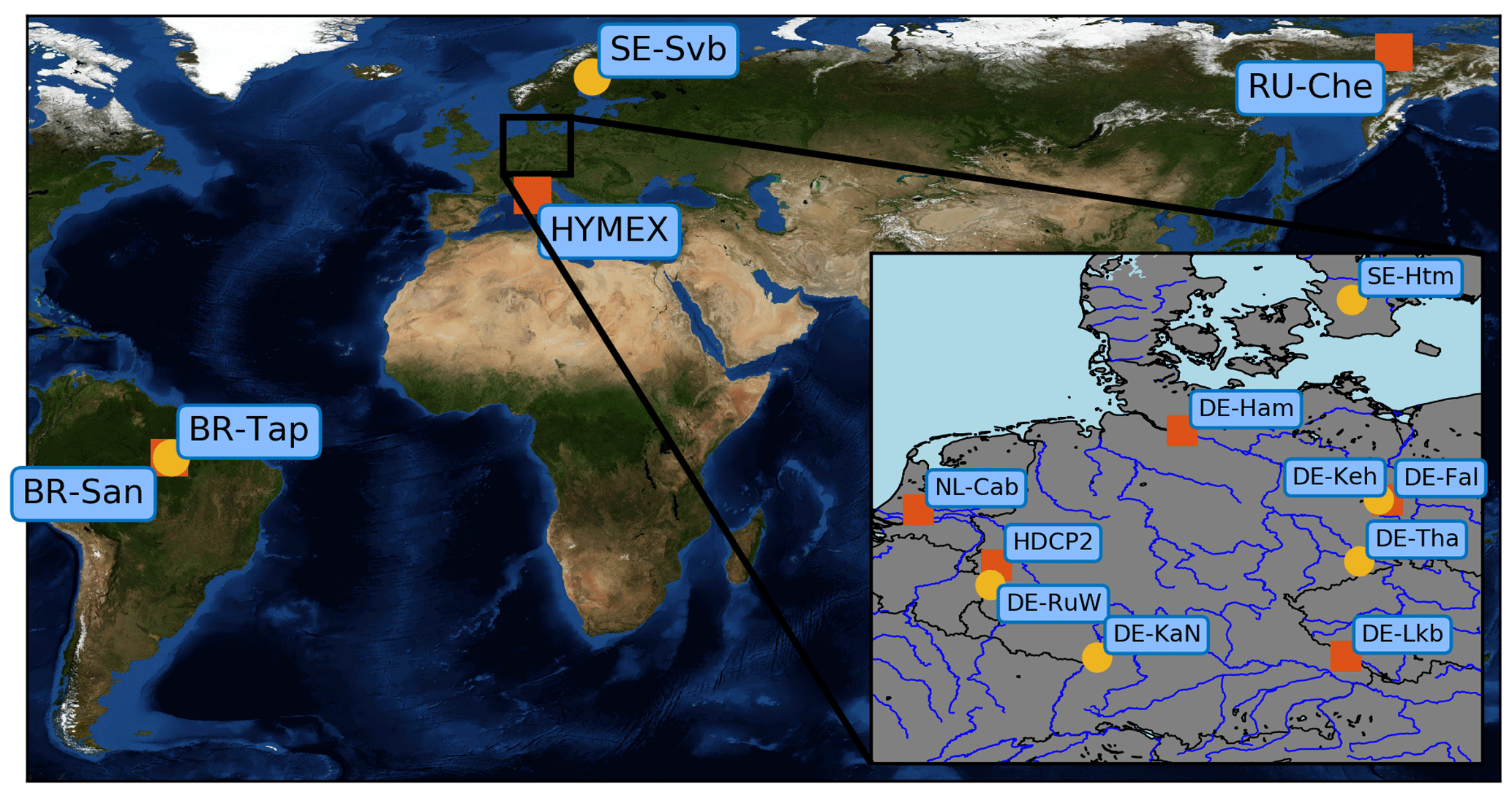
Figure 1Location of the stations that provided data for this study. Station symbols represent low (red square; grasslands, croplands and wetlands) and tall (yellow circle; forest) vegetation. HDCP2 includes the DE-Nie07, DE-Nie13 and DE-Was06 stations, and HYMEX includes the FR-CorX and FR-GiuX stations. Further information can be found in Table A1.

Figure 2The schematic set-up of the meteorological towers used for this study. Available measurements for wind velocity (black, left arm) and temperature (black, right arm) are shown as well as the final measurement height that was used for wind (blue), temperature (yellow) and turbulent fluxes (red). Vegetation height is illustrated in green, and towers with a total height above 80 m are clipped. (“Left arm” and “right arm” in this caption refer to horizontal arms that the instruments are mounted to on a real mast.)
An important step before using data as input for the ANN was to check if the data were compatible with Monin–Obukhov theory, i.e. if an (at least approximate) functional relationship between ζ and the right-hand sides of Eq. (1) was present and if so, how well they were represented by the universal stability functions in Eq. (1). It was found that no relationship existed for some sites. This may have been due to a violation of the assumptions of the Monin–Obukhov theory, such as inhomogeneous terrain around the site or the dependence of the roughness length on the wind direction. Data from these sites were not used further, except for data from the DE-Tha site (see Sect. 4). The remaining stations (see Table 1), which comprised about 113 500 hourly averaged data points in total (see Table 2), were used to train and validate the networks. For these stations, agreement was generally better for temperature than for wind; furthermore, agreement was better for unstable than for stable stratification, an observation which is often mentioned in the literature.
Data were preprocessed before they were presented to the ANN. Input and output data were normalised according to their extrema to the interval [0,1] (see Table 3). Furthermore, weak wind situations with wind speeds below 0.3 m s−1 were filtered out. Because of the large scatter of wind and temperature gradients under atmospheric conditions with absolute heat fluxes below 10 W m−2 or small scaling wind speeds ( m s−1), such data were excluded. Finally, the signs of the temperature scale θ* and the potential temperature gradient had to be the same; this meant excluding counter-gradient fluxes which can be observed over forests (Denmead and Bradley, 1985) and ice (Sodemann and Foken, 2005) but violate the assumptions of MOST (Foken, 2017a, b).
2.5 Cross-validation and generalisation
Trained networks were validated using k-fold cross-validation (Kohavi, 1995; Andersen and Martinez, 1999) to prevent overfitting (Domingos, 2012). Overfitting originates from the trade-off between minimising the error for given data and maximising performance for new unknown data (Chicco, 2017). In the first experiment, the full data set is divided into k=6 subsets using a random data split with approximately equal size first. Cyclically, one subset is kept for independent testing, the remaining k−1 subsets are used for training and validation. Using this experiment, we can show that ANNs are able to learn from the data and to represent their characteristics. In the second experiment, we go one step further and check if the ANNs found can handle not only unknown data but also completely new stations that were not previously used, i.e. if they are able to generalise. For this experiment, we decided to validate trained models using the NL-Cab station and to then test the best ANNs on the DE-Keh station, which had been left out in the training and validation phases of this experiment (see stations details in Sect. 2.4). For these two stations, the MOST method performed best; thus, they present a strong challenge for the ANNs with respect to achieving similar quality.
2.6 ANN set-up and the selection of the best ANN
Neural networks are very flexible in terms of the number of layers, the number of nodes, the error metrics, the training method, the activation function and so on; thus, a series of sensitivity runs were performed, which always consisted of a training and a validation phase. To find an optimal network architecture, we varied the following parameters:
-
the number and type of input variables,
-
the number of hidden layers (one or two) and
-
the total number of nodes in the hidden layer(s) (between 1 and 14).
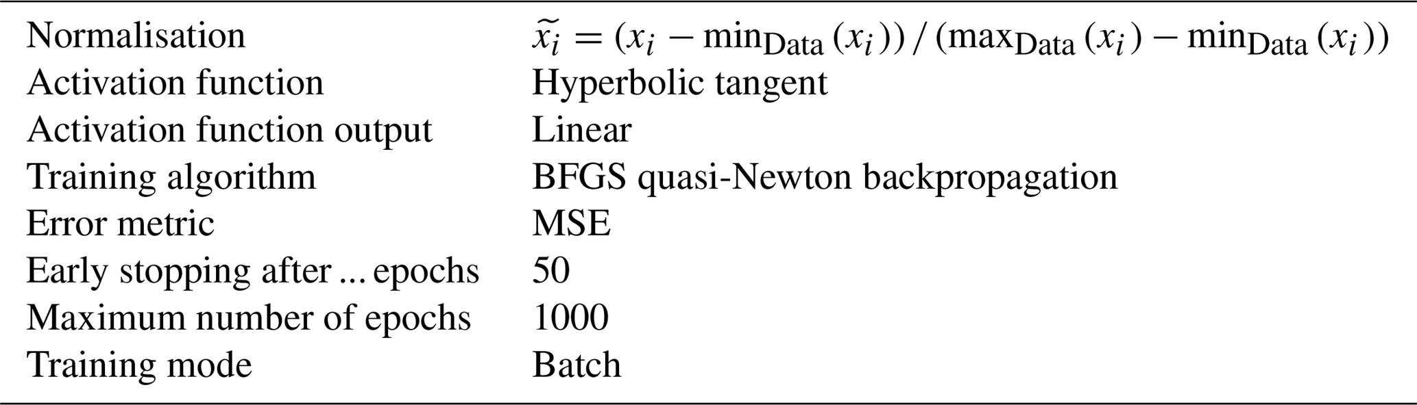
To avoid an excessive number of sensitivity runs, the parameters listed in Table 3 were kept fixed based on recommendations in the literature (Zhang, 2008; Kruse et al., 2016). Training was carried out in batch mode; therefore, the network's weights were adjusted after each epoch. Training ended at most after 1000 epochs or if the error on the validation data increased for 50 successive epochs (early stopping). In the latter case, the state of the trained network with the lowest error for the validation data (and not the early stopping state) was set as final state. We tested network architectures with six- and seven-element input vectors. The six-element input vector consisted of the wind speed and potential temperature averages over the two heights, the vertical gradients of wind and potential temperature, and their ratio and a classifier to distinguish between low (cveg=0) and tall (cveg=1) vegetation. For the seven-element input vector, we replaced the temperature gradient by its absolute value and added an additional input node describing the sign of the potential temperature gradient. In both cases, the target vector remained a two-element vector consisting of the wind scale u* and the temperature scale θ*. As mentioned above, we experimented with ANNs with one and two hidden layers. For the ANNs with one hidden layer, we varied the number of neurons in the hidden layer from one to twice the size of the input layer. For ANNs with two hidden layers, the number of neurons in each layer was increased up to the number of input neurons.
Table 1Station information for the meteorological towers selected for training and validation (see Sect. 2.4); a list of all stations is given in Table A1. Land usage classification follows the International Geosphere–Biosphere Programme (IGBP) standards: evergreen needle-leaf forests (ENF), grasslands (GRA), permanent wetlands (WET) and croplands (CRO).

Table 2Time series information for the meteorological towers selected for training and validation. Count and availability are measured at hourly intervals and not at the original resolution of each time series.
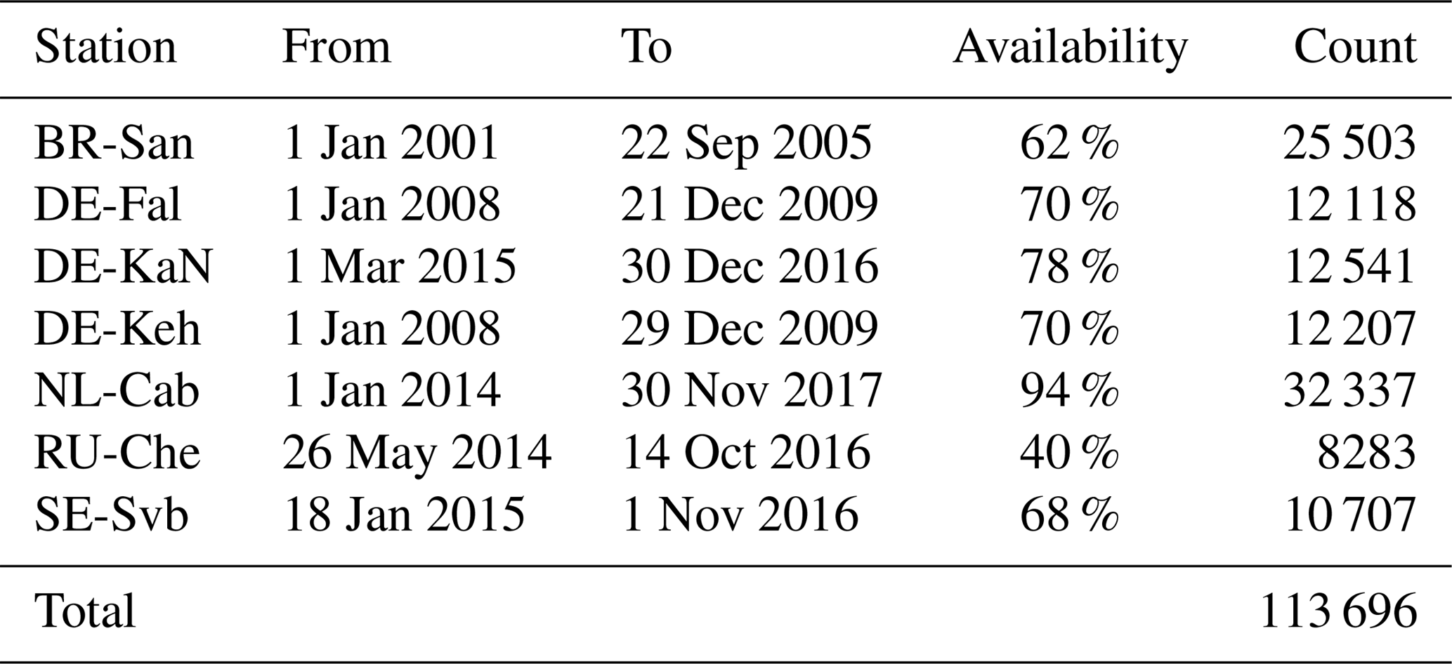
Table 3Fixed network parameters for training (following Zhang, 2008; Kruse et al., 2016).
All networks were trained to minimise the overall (sum of u* and θ*) MSE on normalised data from Eq. (6). To compare the different ANNs, we used the root-mean-squared error (RMSE) , the mean absolute error (MAE)
and the Pearson correlation coefficient (r)
where and are the averages of the jth net output and the target value with and .
When ANNs are to be used in climate models, one has to find a trade-off between two aspects: on the one hand, the model should perform well according to the quality metrics described above, on the other hand, a superior model in terms of small errors but with higher computational demands may not be the best choice for use in climate models where reducing computing time is a very high-priority criterion. For ANNs, computing time normally increases with the complexity of a network, i.e. with its size. Therefore, we also tested ANNs with smaller-than-optimal numbers of neurons in view of this trade-off. To find smaller networks that possibly required less computing time, we looked at networks that met the requirement that the size of each hidden layer was less or equal to the size of the input layer nI minus 1:
This condition was found after some experimentation and is somewhat arbitrary, but there is no hard rule defining the simplicity of a model. We will refer to ANNs that satisfy this condition as “simple networks”.
As described in Sect. 2.5, ANNs are always trained on the training data set only and validated on a disjoint validation data set. If the MSE on the validation set rises continuously, training is stopped to prevent overfitting (early stopping). Following this training and validation stage, the ability of the selected ANNs to generalise is tested on data that are completely new to the ANNs. All in all, more than 100 000 networks were trained and tested this way.
3.1 Effect of data splitting
The validation results from ANNs with six inputs and one single hidden layer trained under six-fold cross-validation with random data splitting are shown in the box-and-whiskers plot in Fig. 3 as a function of the number of hidden neurons. One can see that the validation MSE decreases with the increasing number of hidden neurons and has already reached an asymptotic value of about 0.008 with six to seven neurons. Furthermore, the scatter of the MSE is quite small, meaning that the quality of the results from ANNs trained on different sets varies only slightly.
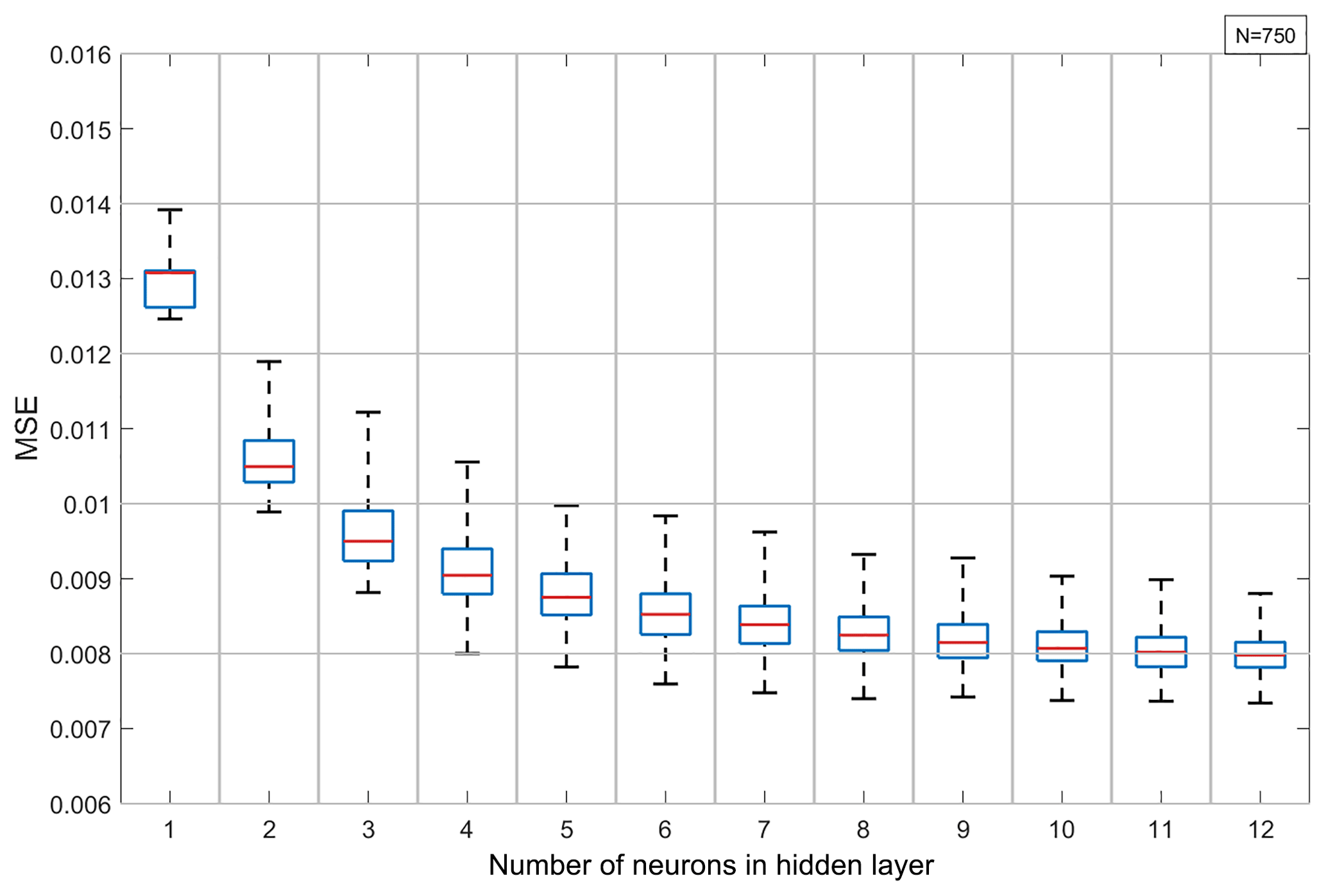
Figure 3Network with six inputs and one hidden layer under six-fold cross-validation: the MSE of the network trained on the validation data set using random data splitting as a function of the hidden layer size. Whiskers indicate the interquartile range, and each box summarises the results from 750 single networks.
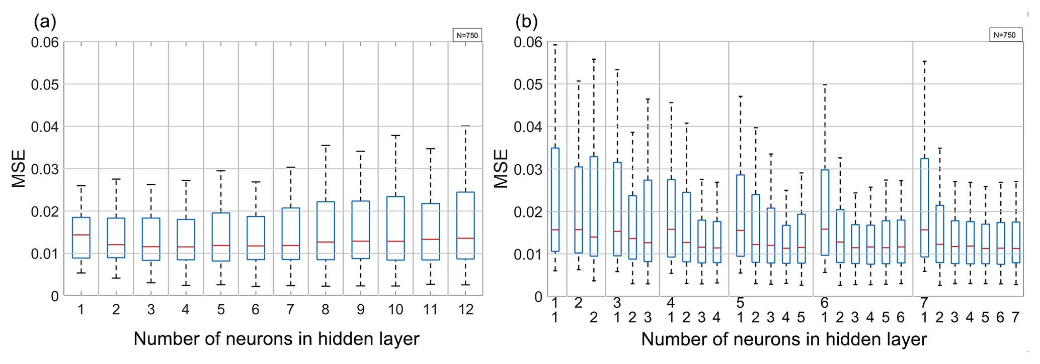
Figure 4The validation MSE of trained networks using a station-wise data split as a function of the hidden layer size for (a) the network with six inputs and one hidden layer (left), and (b) the network with seven inputs and two hidden layers (right). The numbers on the bottom axis of (b) indicate the number of neurons in the first (top row) and second (bottom row) hidden layer. Values for the other networks considered are similar. Whiskers indicate the length of interquartile range, and each box summarises the results from 750 single networks.
If the training data are not split randomly but undergo a station-wise split, a larger MSE and a considerably larger scatter of the MSE results are found. Comparing Fig. 4 with Fig. 3 shows that the MSE roughly doubles, whereas scatter increases by about a factor of 10, almost independent of the network architecture. Conversely, increasing the network size does not necessarily imply a lower MSE. Using two hidden layers slightly reduces the median and error minimum, but also increases the MSE spread. The comparison of Fig. 3 with Fig. 4 also shows that the station-wise error minima are comparable to those obtained from a random data split. In both types of validation, ANNs with one and two hidden layers are not significantly different.
All in all, comparing Fig. 3 with Fig. 4 shows that the station-wise data split substantially reduces the ANN performance. This implies that using not enough stations as well as station-wise training impairs the generalisation of learned relationships between inputs and target values. Possible reasons for this may be the tendency of the ANNs to overfit training data by memorising relationships and local effects contaminating the validity of MOST, such as unideal positioning of sites or unideal atmospheric conditions. These findings confirm the need for independent testing with data that is unknown to the ANN in order to estimate the ANNs real ability to generalise. This will be discussed in the next section.
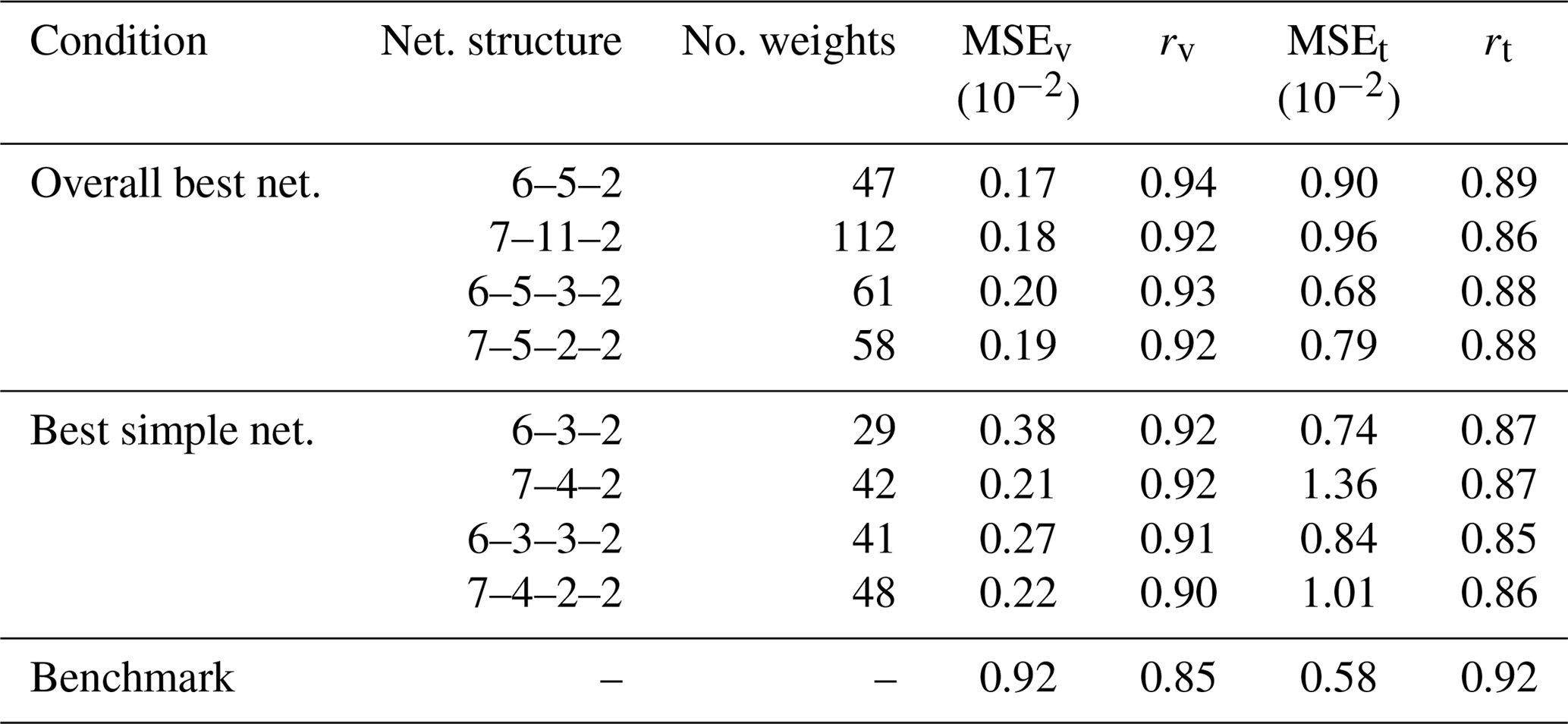
Table 4Performance results of the overall best network and the best simple network. MSE and r are measured on normalised data and are non-dimensional. MSEv and rv are calculated on validation data, and MSEt and rt are calculated on test data. The performance of the MOST method (the “Benchmark”) is also shown.
3.2 Generalisation to unknown data
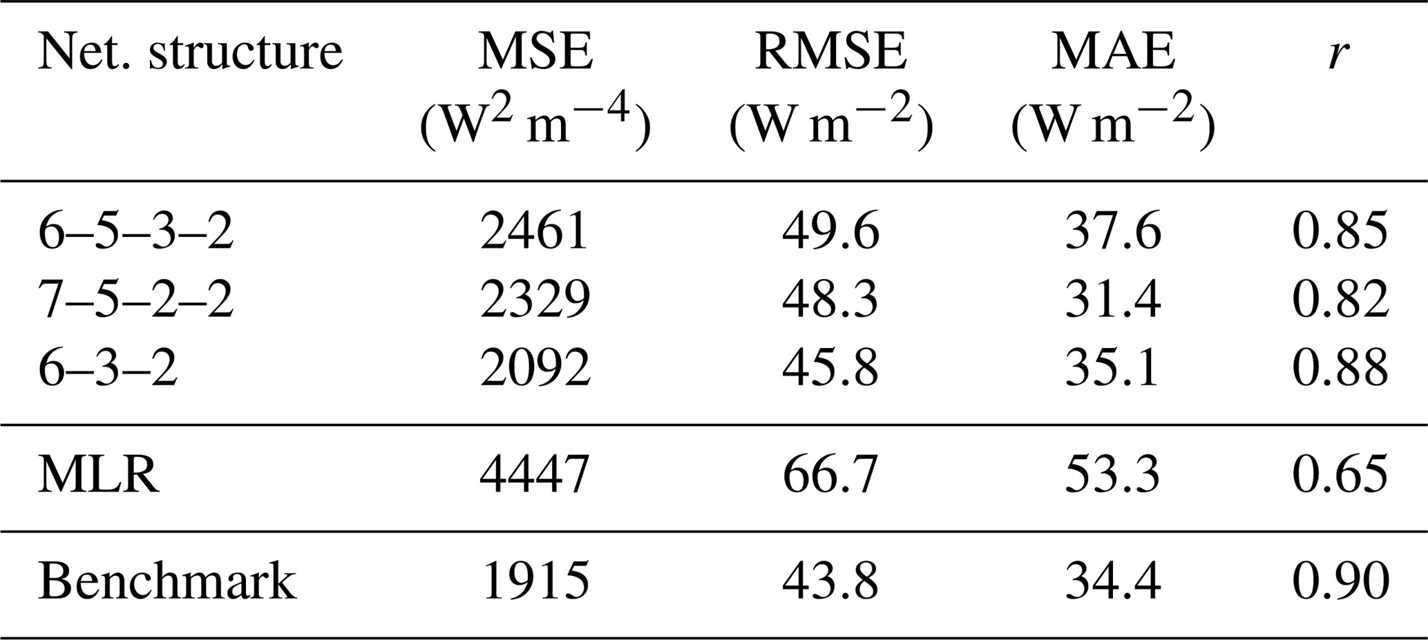
After showing that ANNs are able to extract u* and θ* from training data successfully, our next step is to assess how the ANNs found in the previous section can handle input from stations which were not used for training or validation, i.e. data completely unknown to them; this simulates the situations in which ANNs would be used in climate models (where grid points play the role of stations). To test this, we choose the NL-Cab station for validation and DE-Keh as the unknown station. We selected these two stations because the MOST method performed best for these stations; therefore it is a strong challenge for the ANNs to produce equivalent results. The results of the networks that perform best on the validation set are summarised in Table 4, where we compare the ANNs according to the increasing complexity of their network architecture. For comparison, and in view of reducing CPU time, we also show the results of the best simple networks (as defined in Sect. 2.6) in this table. Table 4 shows that all ANNs perform better than the MOST method on the validation data set (NL-Cab), in terms of the MSE and correlation coefficient (r). Applying these ANNs to the test data set (DE-Keh) results in an increased MSE and a lower correlation coefficient, whereas the MOST method performs better on the test data set. Among the ANNs, the 6–5–3–2 ANN displayed the best test performance with a MSE of , but the simpler 6–3–2 ANN was second best (also in terms of the MSE); thus, simple networks can be almost as good as larger networks. Networks with seven inputs have no substantial advantage over networks with six inputs in our research. ANNs with two hidden layers perform slightly better on the test data than ANNs with a single hidden layer. The overall correlation between network outputs and target values is quite high (r≥0.85) in all cases.
We also carried out a comparison for the turbulent momentum and heat fluxes and , which are the quantities ultimately needed in climate simulations. Results for the momentum and heat fluxes of three networks that performed well as well as for the MOST method are shown in Figs. 5 and 6 and in Tables 5 and 6, respectively. In the tables we also show the results of the multivariate linear regression (MLR) described in Sect. 2.3. Both ANNs, MLR and the standard method tend to underestimate larger momentum fluxes, but differences among ANNs are quite small. The best agreement is achieved with the 6–5–3–2 ANN, which is almost as good as the standard method.
Regarding the heat flux, the differences between the ANNs are again relatively small, but the ANNs as well as the standard method tend to overestimate the heat fluxes, whereas MLR underestimates them (not shown). The best results are obtained with the 6–3–2 ANN. For heat flux, the 7–5–2–2 ANN behaves quite differently to the other ANNs. It produces two distinct states, one around −30 W m−2 and the other from 50 to 200 W m−2; as a result, r is reduced but the MAE is lowest for this 7–5–2–2 ANN. Thus, the 7–5–2–2 ANN acts more like a dichotomous classifier of stability rather than the continuous regression we are looking for. As for the momentum fluxes, the ANNs shows considerably better performance than the regression model. These results reiterate that smaller networks can be as good as or even better than larger networks.
Table 5Performance of networks vs. multivariate linear regression (MLR) and the MOST method (“Benchmark”) for momentum flux at the DE-Keh station.
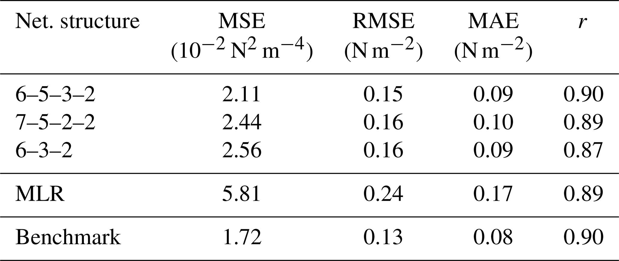
All ANNs show considerably better performance than the multivariate linear regression model. This is not really surprising, as the scaling quantities to be approximated are non-linear functions of stability (Arya, 2001), meaning that an ANN with a non-linear activation function would be expected to perform better than any linear model; as Tables 5 and 6 show, this is the case, even for the small 6–3–2 ANN with one hidden layer.

Figure 5Plots of network output vs. target values for momentum flux on unknown test data (DE-Keh). The 6–3–2 ANN (a), 6–5–3–2 ANN (b), 7–5–2–2 ANN (c) and the MOST method (d) are shown. Contours represent the kernel density estimates of the two-dimensional probability density distribution with the 95th, 75th, 25th and 5th percentiles (yellow contours – starting from the outermost contour) and the 50th percentile (green contour).
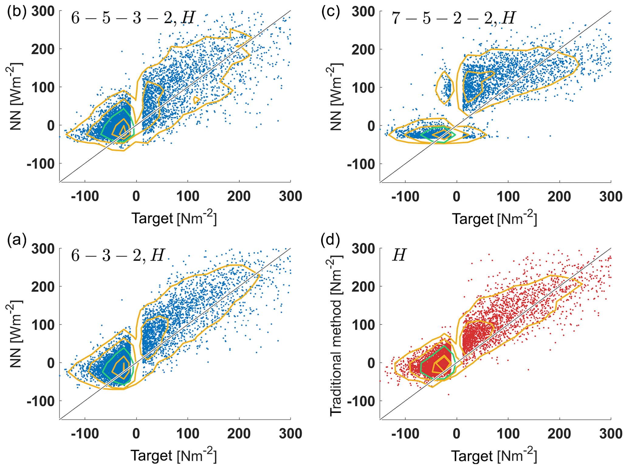
Figure 6Plots of network output vs. target values for heat flux on unknown test data (DE-Keh). The 6–3–2 ANN (a), 6–5–3–2 ANN (b), 7–5–2–2 ANN (c) and the MOST method (d) are shown. Contours represent the kernel density estimates of the two-dimensional probability density distribution with the 95th, 75th, 25th and 5th percentiles (yellow contours – starting from the outermost contour) and the 50th percentile (green contour). The vertical gap is due to the exclusion of heat fluxes between ±10 W m−2.
Table 6Performance of networks vs. multivariate linear regression (MLR) and the MOST method (“Benchmark”) for heat flux at the DE-Keh station.
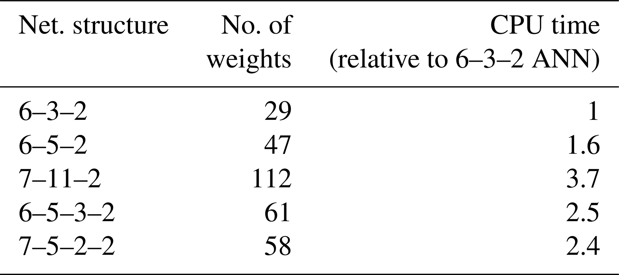
A comparison of the CPU time required by the different ANNs relative to 6–3–2 ANN is shown in Table 7. The table shows that the increase in computational demand is approximately proportional to the number of weights (as could be expected), and therefore increases considerably when two-layer networks are used. As the discussion above shows, these costs are not reflected in a substantially higher quality of results.
We can conclude that generalisation entails a reduced performance of the ANNs with quite small differences between the various ANNs. The performance of the ANNs is comparable to the MOST method, and the simplest 6–3–2 network has the best score in terms of accuracy and computational efficiency.
Table 7Relative computational demand of the ANNs discussed in the text.
As already mentioned, our goal is to replace the MOST method for calculating fluxes with an ANN in the land surface component of climate models; in doing so, we expect more flexibility, accuracy and to possibly save CPU time. The results presented in the previous section indicate that from an accuracy and computational efficiency point of view, the 6–3–2 ANN seems to be most suitable for implementation into a land surface model (LSM). This ANN is shown in Fig. 7.
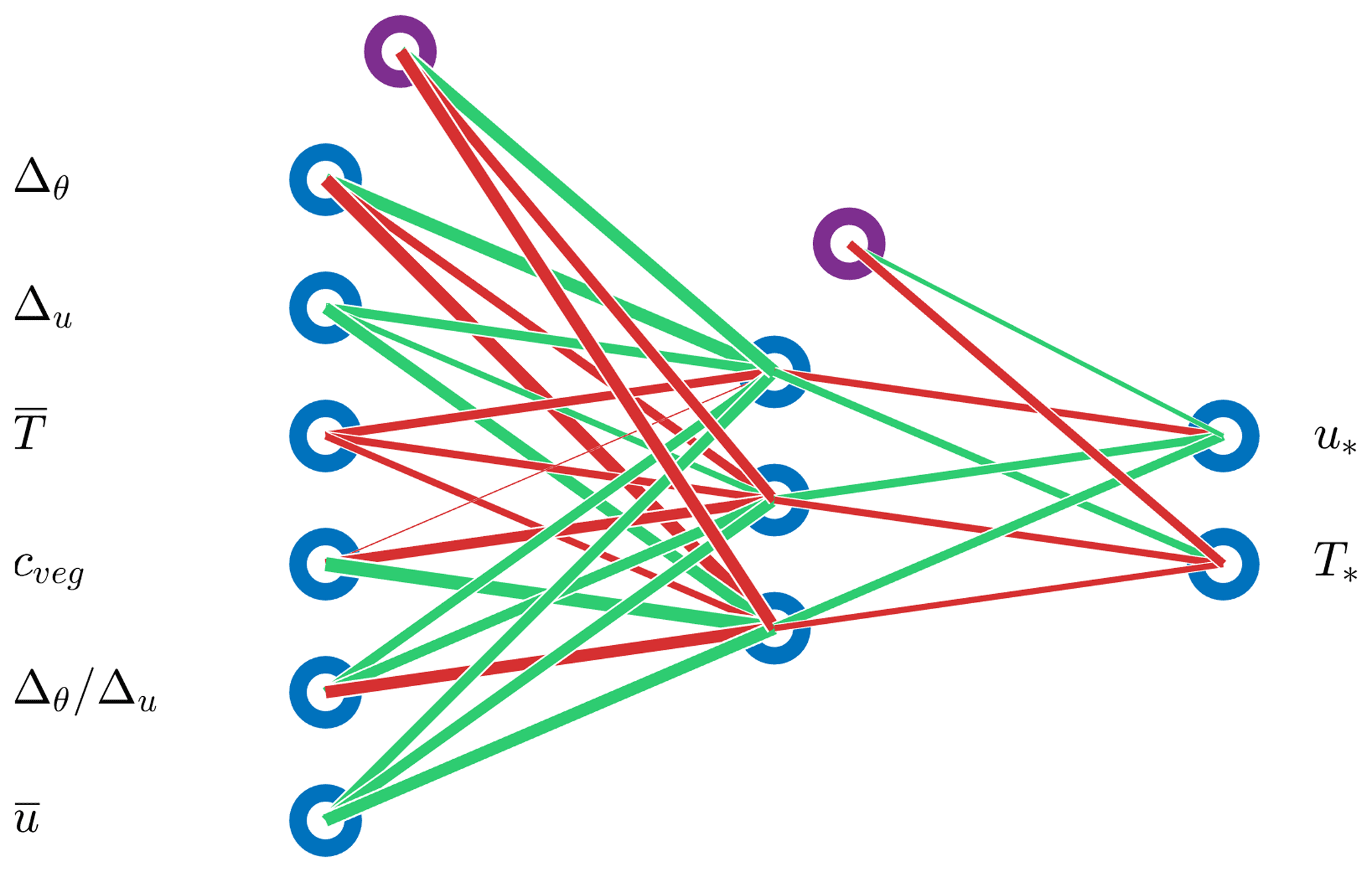
Figure 7The architecture of the 6–3–2 ANN implemented in the land surface model. Input is described in Sect. 2.6. Purple circles are bias neurons.
We implemented the 6–3–2 ANN with weights as obtained in the previous sections in a stand-alone version of the one-dimensional LSM Veg3d (Braun and Schädler, 2005); this replaced the routine using the MOST method to calculate the scaling quantities u* and θ*. Here, we refer to the LSM version with the original MOST version as the reference version. Input data for the ANN and data normalisation were the same as described in Sect. 2.4 and output was analogously de-normalised. As the LSM requires the moisture flux in addition to the momentum and heat fluxes, we calculated the scaling specific humidity q* as proportional to θ* following the standard procedure used in boundary layer meteorology (Arya, 2001). Meteorological input for the LSM consisted of 30 min values of short- and longwave radiation, wind speed, temperature, specific humidity and air pressure at two heights; soil type and land use were also additionally prescribed. In the present study, the meteorological data were only available for the DE-Fal station for the year 2011 and for the DE-Tha site for the year 1998. For comparison with observations, time series of heat and moisture fluxes as well as soil temperature and soil moisture in the upper soil layers were available, so that the effect of the ANN on the soil component could also be assessed. We performed the comparison with data from the DE-Fal (grassland, year 2011) and DE-Tha (evergreen needle-leaf forest, year 1998) stations for years which had not yet been used for training or validation; thus, the data were new to the ANN in the sense that time periods were used which had not been previously used for training and validation. The DE-Tha station had not been used at all up until this point, as the other sites selected in Sect. 2.4 were more consistent with MOST than DE-Tha and because the DE-Tha time series covered only 1 year. We compared the RMSE and the correlation coefficient of the calculated values with those observed for the reference version and the ANN version. Additionally, we compared the required CPU times. The results of the comparison are shown in Tables 8 and 9.
Table 8Comparison of the reference version with the ANN version of Veg3d for the DE-Fal grassland station. H denotes the heat flux, M is moisture flux, Ts is soil temperature and ws is soil moisture.
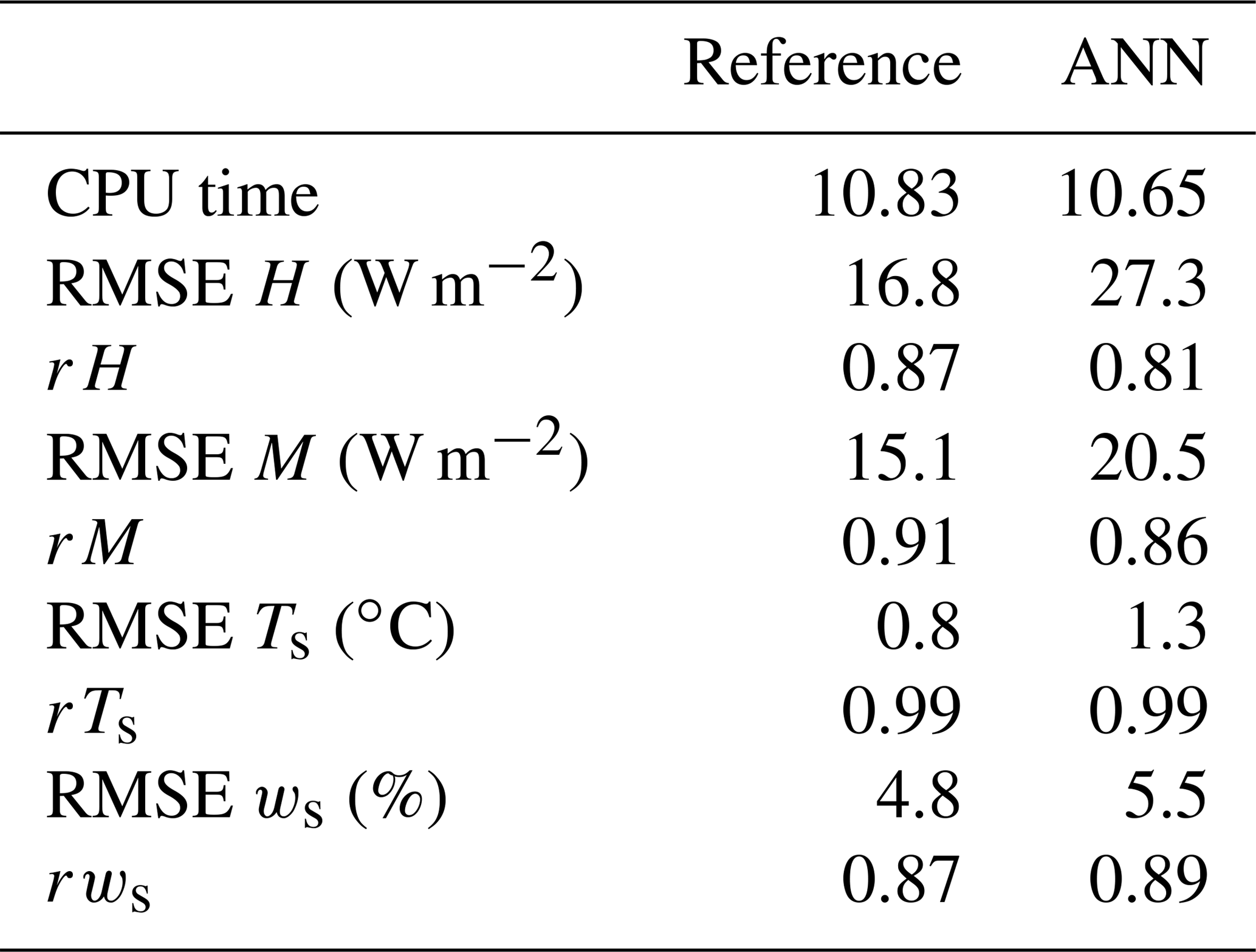

Especially for grassland, the results of the reference version are very good in terms of RMSE and correlation coefficients, and it is difficult for the ANN version to outperform this. However, the results show that the ANN version is able to produce results of a similar quality to the reference version for the fluxes as well as for soil temperature and soil moisture. For tall vegetation, RMSEs are larger and the correlation coefficients are lower; but the differences between the ANN version and the reference version are even smaller than for grassland, and the ANN version even outperforms the reference version for soil moisture. In terms of fluxes, the reference version is generally slightly better. Regarding CPU time, there are only minor differences, although we expected the ANN version to be faster. However, due to the small prognostic time step used, once initialised, the reference version does not need to do more than one iteration to find a solution to the non-linear equation and to update the scaling quantities in most cases; hence, the expensive iteration is reduced considerably. In summary, as a result of this first comparison, it can be concluded that the ANN version works as well as the reference version.
We used an ANN (more precisely, a MLP) to obtain the scaling quantities u* and θ* as defined in MOST; these parameters are used in weather and climate models to calculate the turbulent fluxes of heat and momentum in the atmospheric surface layer. To train, validate and test the neural network, a large set of worldwide observations was used, which represented tall (forests) and low vegetation (grassland and agricultural terrain). A quality assessment of the data sets showed that not all of them were compatible with MOST, so only 7 of the 20 initial data sets could be used.
Sensitivity studies were performed with different sets of input parameters, data sampling methods and network architectures; validation was undertaken using 6-fold cross validation. An important part of the overall network validation was to assess the ability of the network to generalise, i.e. to produce acceptable output if input were data from stations that were completely unknown to the network. These studies showed that even a relatively small 6–3–2 network with six input parameters and one hidden layer yields satisfying results in terms of the RMSE and correlation coefficient. With respect to the trade-off between the quality of results and the computational efficiency, this network performed best.
We could show that the results of the ANN were equivalent to the standard method in all of the tests we performed. A final validation with the heat and momentum fluxes instead of the scaling quantities showed that the MOST method and the ANN approach were also almost equal in terms of quality in this case, with the 6–3–2 ANN performing best. Furthermore, we could show that the ANNs outperform a multivariate linear regression model with the same input and output variables and training and test data. This could be expected, as the stability functions are non-linear functions; therefore, even a small ANN with one hidden layer and a non-linear activation function could be expected to perform better than any linear model. An implementation of the 6–3–2 ANN into an existing LSM showed that the ANN version gives results equivalent to the standard implementation, sometimes even with even higher correlations. However, no decrease in the required CPU time was found.
In summary, it could be shown that even at this stage, an ANN gives results comparable in quality to the MOST method. Some obvious improvements will include more and better differentiated land use classes (e.g. water and urban areas) and more situations of strong stratification. Next steps will include more experiments with the input parameters (e.g. including a time lag) and some fine tuning to improve the computational efficiency (e.g. using different activation functions). We intend to implement and test the neural network routine in a three-dimensional regional climate model (RCM). We expect to save about 5 % of the CPU time, taking parallelisation into account. This may not seem like much, but RCMs in particular are very expensive to run (climatologically relevant multidecadal simulations at high resolution can take several tens of weeks on a high performance system), so every saving counts. The implementation will require the ANN to learn some additional land use types, such as urban areas or water surfaces. If these tests are positive, this would pave the way for replacing other “uncertain” components of climate models (e.g. cloud microphysics, sea ice) with neural network subroutines, similar to the work described in Sarghini et al. (2003) and Vollant et al. (2017), which would increase flexibility and save CPU time. The main hindrance to this undertaking is the current lack of suitable training and validation data. An alternative to “real”' data may be the use of data from more detailed models such as LES or urban climate models.
A MATLAB script (run.m) that runs the 6–3–2 network with a sample data set (DE-KaN.dat) can be found at http://doi.org/10.23728/b2share.36ef510c515c4a00bb963113647e44a9.
The data for this study were obtained from the sources mentioned in the acknowledgements.
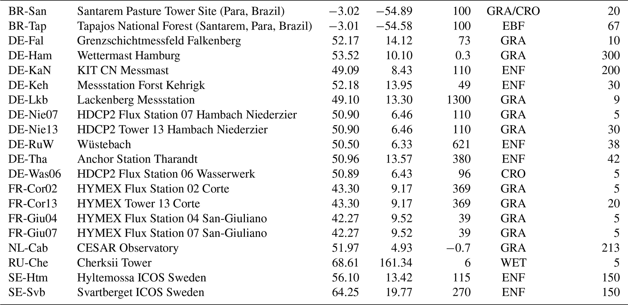
Table A1Station information for all of the meteorological towers utilised in the study. Land use classification follows the International Geosphere–Biosphere Programme (IGBP) standards: evergreen needle-leaf forests (ENF), evergreen broadleaf forests (EBF), grasslands (GRA), permanent wetlands (WET) and croplands (CRO).
LL was responsible for data collection, quality checks and data preprocessing. LL also trained, validated and generalised the ANNs, performed the MLR analysis and made the comparisons with the MOST method. GS implemented the 6–3–2 network in a land surface model and carried out performance measurements in terms of result quality and CPU time. GS prepared the paper with contributions from LL.
The authors declare that they have no conflict of interest.
The authors would like to thank following people and institutions for providing station data: Martin Kohler and Rainer Steinbrecher (Karlsruhe Institute for Technology), Mathias Göckede, Olaf Kolle and Fanny Kittler (Max Planck Institute for Biogeochemistry Jena), Frank Beyrich (German Weather Service), Ingo Lange (University of Hamburg), Clemens Drüe (University of Trier), Marius Schmidt (Forschungszentrum Jülich) and Thomas Grünwald (TU Dresden). In addition, data from the following sources were collected and used: the Integrated Carbon Observation System Sweden (ICOS), the Cabauw Experimental Site for Atmospheric Research (CESAR) database, the Oak Ridge National Laboratory Distributed Active Archive Center (ORNL DAAC) and the University Corporation for Atmospheric Research (UCAR). We thank the two anonymous reviewers and the editor for their helpful comments and suggestions. Finally, we acknowledge support from the KIT-Publication Fund of the Karlsruhe Institute of Technology.
The article processing charges for this open-access publication were covered by a Research Centre of the Helmholtz Association.
This paper was edited by Chiel van Heerwaarden and reviewed by two anonymous referees.
Andersen, T. and Martinez, T.: Cross validation and MLP architecture selection, in: IJCNN'99. International Joint Conference on Neural Networks. Proceedings, Washington, DC, USA, 10–16 July 1999, IEEE, 3, 1614–1619, 1999. a
Arya, P. S.: Introduction to micrometeorology, in: International Geophysics Series, San Diego, Calif., Academic Press, vol. 79, 2001. a, b, c, d
Braun, F. and Schädler, G.: Comparison of Soil Hydraulic Parameterizations for Mesoscale Meteorological Models., J. Appl. Meteorol., 44, 1116–1132, 2005. a
Broyden, C. G.: The Convergence of a Class of Double-rank Minimization Algorithms 1. General Considerations, IMA J. Appl. Math., 6, 76–90, https://doi.org/10.1093/imamat/6.1.76, 1970. a
Businger, J. A., Wyngaard, J. C., Izumi, Y., and Bradley, E. F.: Flux-Profile Relationships in the Atmospheric Surface Layer, J. Atmos. Sci., 28, 181–189, https://doi.org/10.1175/1520-0469(1971)028<0181:FPRITA>2.0.CO;2, 1971. a
Chicco, D.: Ten quick tips for machine learning in computational biology, BioData Min., 10, 35, https://doi.org/10.1186/s13040-017-0155-3, 2017. a
Comrie, A. C.: Comparing neural networks and regression models for ozone forecasting, JAPCA J. Air Waste Ma., 47, 653–663, 1997. a
Denmead, O. T. and Bradley, E. F.: Flux-Gradient Relationships in a Forest Canopy, in: The Forest-Atmosphere Interaction: Proceedings of the Forest Environmental Measurements Conference held at Oak Ridge, Tennessee, 23–28 October 1983, edited by: Hutchison, B. A. and Hicks, B. B., Springer Netherlands, Dordrecht, 421–442, 1985. a
Domingos, P.: A few useful things to know about machine learning, Commun. ACM, 55, 78–87, 2012. a
Elkamel, A., Abdul-Wahab, S., Bouhamra, W., and Alper, E.: Measurement and prediction of ozone levels around a heavily industrialized area: a neural network approach, Adv. Environ. Res., 5, 47–59, 2001. a, b
Fletcher, R.: A new approach to variable metric algorithms, Comput. J., 13, 317–322, 1970. a
Foken, T.: Micrometeorology, SpringerLink: Bücher, Springer, Berlin, Heidelberg, 2nd edn., 2017a. a
Foken, T.: Energy and Matter Fluxes of a Spruce Forest Ecosystem, vol. 229, Springer, International Publishing, 2017b. a
Gardner, M. and Dorling, S.: Neural network modelling and prediction of hourly NOx and NO2 concentrations in urban air in London, Atmos. Environ., 33, 709–719, 1999. a
Gentine, P., Pritchard, M., Rasp, S., Reinaudi, G., and Yacalis, G.: Could machine learning break the convection parameterization deadlock?, Geophys. Res. Lett., 45, 5742–5751, https://doi.org/10.1029/2018GL078202, 2018. a
Goldfarb, D.: A family of variable-metric methods derived by variational means, Math. Comput., 24, 23–26, 1970. a
Gomez-Sanchis, J., Martín-Guerrero, J. D., Soria-Olivas, E., Vila-Francés, J., Carrasco, J. L., and del Valle-Tascón, S.: Neural networks for analysing the relevance of input variables in the prediction of tropospheric ozone concentration, Atmos. Environ., 40, 6173–6180, 2006. a
Högström, U.: Non-dimensional wind and temperature profiles in the atmospheric surface layer: A re-evaluation, Bound.-Lay. Meteorol., 42, 55–78, https://doi.org/10.1007/BF00119875, 1988. a, b
Högström, U.: Review of some basic characteristics of the atmospheric surface layer, Bound.-Lay. Meteorol., 78, 215–246, https://doi.org/10.1007/BF00120937, 1996. a
Hornik, K., Stinchcombe, M., and White, H.: Multilayer feedforward networks are universal approximators, Neural Networks, 2, 359–366, 1989. a
Knutti, R., Stocker, T., Joos, F., and Plattner, G.-K.: Probabilistic climate change projections using neural networks, Clim. Dynam., 21, 257–272, 2003. a
Kohavi, R.: A study of cross-validation and bootstrap for accuracy estimation and model selection, in: IJCAI'95 Proceedings of the 14th international joint conference on Artificial intelligence, Montreal, Quebec, Canada, 20–25 August 1995, 2, 1137–1145, 1995. a
Kolehmainen, M., Martikainen, H., and Ruuskanen, J.: Neural networks and periodic components used in air quality forecasting, Atmos. Environ., 35, 815–825, 2001. a, b
Kruse, R., Borgelt, C., Braune, C., Mostaghim, S., and Steinbrecher, M.: Computational intelligence: a methodological introduction, Springer, London, 2016. a, b, c
Monin, A. S. and Obukhov, A. M.: Basic laws of turbulent mixing in the surface layer of the atmosphere, Tr. Akad. Nauk SSSR Geophiz. Inst., 24, 163–187, 1954. a, b
Rojas, R.: Neural networks: a systematic introduction, Springer Science & Business Media, Berlin, 2013. a
Sarghini, F., de Felice, G., and Santini, S.: Neural networks based subgrid scale modeling in large eddy simulations, Comput. Fluids, 32, 97–108, 2003. a, b, c
Shanno, D. F.: Conditioning of quasi-Newton methods for function minimization, Math. Comput., 24, 647–656, 1970. a
Sodemann, H. and Foken, T.: Special characteristics of the temperature structure near the surface, Theor. Appl. Climatol., 80, 81–89, 2005. a
Vollant, A., Balarac, G., and Corre, C.: Subgrid-scale scalar flux modelling based on optimal estimation theory and machine-learning procedures, J. Turbul., 18, 854–878, https://doi.org/10.1080/14685248.2017.1334907, 2017. a, b, c
Zhang, G. P.: Neural Networks For Data Mining, in: Soft Computing for Knowledge Discovery and Data Mining, edited by: Maimon, O. and Rokach, L., Springer US, Boston, MA, chap. 21, 17–44, https://doi.org/10.1007/978-0-387-69935-6_2, 2008. a, b, c, d, e