Bayesian inference and predictive performance of soil respiration models in the presence of model discrepancy

Bayesian inference of microbial soil respiration models is often based on the assumptions that the residuals are independent (i.e., no temporal or spatial correlation), identically distributed (i.e., Gaussian noise), and have constant variance (i.e., homoscedastic). In the presence of model discrepancy, as no model is perfect, this study shows that these assumptions are generally invalid in soil respiration modeling such that residuals have high temporal correlation, an increasing variance with increasing magnitude of CO₂ efflux, and non-Gaussian distribution. Relaxing these three assumptions stepwise results in eight data models. Data models are the basis of formulating likelihood functions of Bayesian inference. This study presents a systematic and comprehensive investigation of the impacts of data model selection on Bayesian inference and predictive performance. We use three mechanistic soil respiration models with different levels of model fidelity (i.e., model discrepancy) with respect to the number of carbon pools and the explicit representations of soil moisture controls on carbon degradation; therefore, we have different levels of model complexity with respect to the number of model parameters. The study shows that data models have substantial impacts on Bayesian inference and predictive performance of the soil respiration models such that the following points are true: (i) the level of complexity of the best model is generally justified by the cross-validation results for different data models; (ii) not accounting for heteroscedasticity and autocorrelation might not necessarily result in biased parameter estimates or predictions, but will definitely underestimate uncertainty; (iii) using a non-Gaussian data model improves the parameter estimates and the predictive performance; and (iv) accounting for autocorrelation only or joint inversion of correlation and heteroscedasticity can be problematic and requires special treatment. Although the conclusions of this study are empirical, the analysis may provide insights for selecting appropriate data models for soil respiration modeling.

1 Introduction

Developing accurate soil respiration models is important for realistic projection of global carbon (C) cycle, as global soils store 2300 Pg carbon, an amount more than 3 times that of the atmosphere (Schmidt et al., 2011), and release 60–75 Pg C yr⁻¹, about 7 times more CO₂ to the atmosphere than all anthropogenic emissions (Le Quéré et al., 2014). The major work on soil respiration modeling has been focused on advancing knowledge about model inputs and calibration data (e.g., Janssens et al., 2003; Peters et al., 2007; Scott et al., 2009; Barron-Gafford et al., 2011; Hilton et al., 2014) and on developing more advanced models to better represent soil microbial processes (e.g., Schimel and Weintraub, 2003; Allison et al., 2010; Davidson et al., 2011; Wieder et al., 2013, 2015; Xu et al., 2014; Zhang et al., 2014). Integration of data and models is indispensable for improving predictability of the terrestrial carbon cycle, and statistical modeling is a vital tool for the model–data integration (Luo et al., 2011, 2014; Wieder et al., 2015). In addition, use of state-of-the-art statistical methods is necessary to accurately quantify uncertainty in parameters and structures of soil respiration models for the improvement and practical use of the models (Katz et al., 2013). A data model, also known as a residuals model or an error model, is used to characterize residuals (i.e., the difference between data and corresponding model simulations). While a large number of data models have been used (e.g., Elshall et al., 2018; Scholz et al., 2018), to our knowledge, a comprehensive and systematic evaluation of data models for soil respiration modeling has not been reported in the literature.

The objectives of this study are to evaluate the impacts of data models on Bayesian inference and predictive performance of three mechanistic soil respiration models, and to use the evaluation results to make broader recommendations. The three models were developed by Zhang et al. (2014) to simulate the Birch effect (the peak soil microbial respiration pulses in response to episodic rainfall pulses) at the site scale and at a short temporal scale; understanding the Birch effect is important to gain a mechanistic understanding of CO₂ efflux production (Högberg and Read, 2006; Vargas et al., 2011). The models from Zhang et al. (2014) are based on an existing four-carbon-pool model from Allison et al. (2010), but have additional carbon pools and/or explicit representations of soil moisture controls on carbon degradation and microbial uptake rates. The models were calibrated, and Bayesian model selection was used to select the best model (Zhang et al., 2014). However, this effort was based on a single data model. It is unknown whether the best model still remains the best (in terms of reproducing both the calibration data and the cross-validation data) if a different data model is used. In addition, as predictive performance of the models was not evaluated in Zhang et al. (2014), it is unknown if the best model will give the best predictions. These two questions are addressed in this study by considering eight data models and by evaluating predictive performance using cross-validation. The top two models (also the two most high-fidelity models) ranked by Zhang et al. (2014) are considered in this study, and the worst model (also the low-fidelity model) is also considered for comparison. We use the terms model fidelity and model discrepancy interchangeably. Model fidelity refers to the degree of realism of the model regarding representing our scientific knowledge with respect to the real world system; hence a high-fidelity model has less discrepancy. Evaluating predictive performance for the three models with different degrees of fidelity provides more insights than a single model.

Bayesian inference in general uses the Bayes' theorem to update the prior distributions of model parameters to posterior parameter distributions given a likelihood function of data. The mathematical formulation of the (formal and informal) likelihood function requires a probabilistic data model; however, this probability model is intrinsically unknown due to unknown errors in all model components such as model structures, parameters, and driving forces. Bayesian inference of soil respiration models often adopts the assumption of independent, normally distributed, and homoscedastic residuals (e.g., Ahrens et al., 2014; Bagnara et al., 2015, 2018; Barr et al., 2013; Barron-Gafford et al., 2014; Braakhekke et al., 2014; Braswell et al., 2015; Correia et al., 2012; Du et al., 2015, 2017; Hararuk et al., 2014; Hashimoto et al., 2011; He et al., 2018; Keenan et al., 2012; Klemedtsson et al., 2008; Menichetti et al., 2016; Raich et al., 2002; Ren et al., 2013; Richardson and Hollinger, 2005; Steinacher and Joos, 2016; Tucker et al., 2014; Tuomi et al., 2008; Xu et al., 2006; Yeluripati et al., 2009; Yuan et al., 2012, 2016; Zhang et al., 2014; Zhou et al., 2010). These assumptions are conveniently adopted to satisfy the requirement of using an unknown probability model in Bayesian statistics, which was referred to as “a basic dilemma” by Box and Tiao (1992).

Postulating the data models is always based on assumptions about residual statistics, and the most widely used assumptions are paired as follows: (i) independent vs. correlated residuals, (ii) homoscedastic vs. heteroscedastic residuals, and (iii) Gaussian vs. non-Gaussian residuals. For soil respiration modeling few studies have relaxed the non-correlation assumption (e.g., Cable et al., 2008, 2011; Q. Li et al., 2016), the homoscedasticity assumption (e.g., Berryman et al., 2018; Elshall et al., 2018; Ogle et al., 2016; Tucker et al., 2013), and the non-Gaussian and homoscedasticity assumptions (e.g., Elshall et al., 2018; Ishikura et al., 2017; Kim et al., 2014). A recent study by Scholz et al. (2018) relaxed these three assumptions using the generalized likelihood function developed by Schoups and Vrugt (2010). However, few studies have focused on investigating the appropriateness and impact of these assumptions for soil respiration modeling by relaxing the independent residuals assumption (Ricciuto et al., 2011) and the Gaussian residuals assumption (Ricciuto et al., 2011; van Wijk et al., 2008). By relaxing these three assumptions stepwise, to our knowledge this is the first study that systematically evaluates the impact of data model selection on Bayesian inference and predictive performance of soil respiration modeling. In addition, to our knowledge, this is the first soil respiration modeling study that investigates the impact of data models in relation to model fidelity.

Relaxing these three assumptions stepwise results in eight data models, which are shown in details in Sect. 2. For example, combining the assumptions of independent, homoscedastic, and Gaussian residuals leads to the standard least squares data model. This model is the simplest of the eight data models, as it only requires one parameter, i.e., the constant variance of the Gaussian distribution. Note that there is a difference between the soil respiration model parameters and the data model parameters. They can technically be jointly estimated, but one arises from assumptions about soil respiration processes and the other from assumptions about the residuals. Relaxing the homoscedastic assumption to heteroscedastic gives the weighted least squared data model. It is more complex because it has extra parameters to account for multiple variances for multiple data. Whenever one or combinations of the three assumptions (independence, homoscedasticity, and normality) are relaxed, the resulting data models become more complex and require more parameters. Such systematic evaluation of data models (McInerney et al., 2017; T. Smith et al., 2010, 2015) is necessary to evaluate the appropriateness of residuals assumptions and their impacts on Bayesian inference.

The assumptions of heteroscedastic, correlated, and non-Gaussian residuals are accounted for using the method of Schoups and Vrugt (2010) in the following procedure: (i) the correlation is removed from the residuals using an autoregressive model; (ii) the resulting residuals are normalized by a linear model of variance; and (iii) the normalized residuals are characterized using the skew exponential power distribution. The data model parameters (i.e., coefficients of the autoregressive model, the linear variance model, and the skew exponential power distribution) are not specified by users, but are estimated along with the soil respiration model parameters during the Bayesian inference. The skew exponential power distribution is general in that by adjusting the values of its kurtosis and skewness parameters the distribution can produce distributions such as the Laplace distribution (van Wijk et al., 2008; Ricciuto et al., 2011) or the distributions from the study by Tang and Zhuang (2009), which utilized an exponential model with different kurtosis parameters. It is worth pointing out that other methods exist to account for the three assumptions. Evin et al. (2013) suggested accounting for residual heteroscedasticity before accounting for residual autocorrelation. Lu et al. (2013) developed an iterative two-stage procedure to separately estimate physical model parameters and data model parameters. Evin et al. (2014) developed a similar procedure to first estimate model parameters and then estimate heteroscedasticity and autocorrelation parameters. While this study uses the method from Schoups and Vrugt (2010), exploring other methods is warranted in future studies.

After investigating the impacts of the data models on Bayesian inference, this study evaluates the impacts of the data models on the predictive performance of the three soil respiration models. Using random samples generated during the Bayesian inference, a prediction ensemble is produced for each soil respiration model. The ensemble is used to evaluate predictive performance of the models in a stochastic sense by estimating extent to which the models can predict future events. The evaluation in this study is carried out using cross-validation by splitting the CO₂ efflux dataset into two parts for Bayesian inference and cross-validation, respectively. The evaluation of predictive performance is important because different data models may give different parameter distributions and therefore different predictive performance. For example, the study by van Wijk et al. (2008) concluded that the choice of the residual function is crucial to achieve accurate model prediction and parameter estimation. Shi et al. (2014) showed that the posterior parameter distributions and predictive performance given by two data models (weighted least squared and skew exponential power distribution after removing heteroscedasticity and autocorrelation) are dramatically different, and a definitive conclusion was drawn that one data model was better than the other. The evaluation of predictive analysis is conducted for the following two cases: (1) the prediction ensemble is generated by random samples of the soil respiration models only (i.e., credible interval), and (2) the prediction ensemble is generated by random samples of not only the soil respiration models but also the data models (i.e., predictive interval). The two cases lead to different conclusions about the predictive performance. It is expected that the evaluation of predictive performance conducted in this study can help select the most appropriate data model to achieve optimal model predictions.

The remainder of the paper is organized as follows. Section 2 starts with a description of the evolving data models and their corresponding likelihood functions used in Bayesian inference, followed by a brief summary of the three soil respiration models. The results of Bayesian inference are discussed in Sects. 3 and 4, addressing the data model implications on parameter estimation and predictive performance, respectively. Section 5 summarizes the key findings and limitations of this study, and provides recommendations for approaching data model selection.

2 Methodology

This section starts with a description of the eight data models that account for the three pairs of assumptions about residuals in a stepwise manner in Sect. 2.1. The data models are used to build the likelihood functions used in Sect. 2.2 for Bayesian inference. The three soil respiration models and observations of CO₂ efflux are described in Sect. 2.3 and 2.4, respectively. Metrics for evaluating predictive performance are presented in Sect. 2.5.

2.1 Data models

This study considers eight evolving data models starting from a data model that assumes independent, homoscedastic, and Gaussian residuals to a data model that relaxes all three assumptions. The eight data models are based on the generic normalized residual,

$$\begin{array}{}\text{(1)}& {\displaystyle }{a}_t={\displaystyle \frac{{\mathit{\epsilon }}_t}{{\mathit{\sigma }}_t}}{a}_t\sim X,\end{array}$$

where ${\mathit{\epsilon }}_t=d_t-Y_t$ is the residual (the difference between data d_t and its corresponding model simulation Y_t) at time or location t, σ_t is the standard deviation of the residual, and X is the probability density function (PDF) of a_t. The eight data models are formulated with different forms of ε_t, σ_t, and X. The standard least square (SLS) data model is

$$\begin{array}{}\text{(2)}& {\displaystyle }{a}_t={\displaystyle \frac{{\mathit{\epsilon }}_t}{{\mathit{\sigma }}_{\mathrm{0}}}}{a}_t\sim N(\mathrm{0},\mathrm{1}),\end{array}$$

where σ_t=σ₀ is a constant for all of the data (i.e., homoscedasticity), and X is the standard normal distribution, N(0,1). The unknown parameter σ₀ is estimated along with the unknown physical model parameters. If σ_t is not a constant (i.e., heteroscedastic), SLS becomes the weighted least squared (WLS) data model. While heteroscedasticity can be accounted for via residuals transformation (e.g., Thiemann et al., 200; T. Smith et al., 2010) or other similar approaches (Gragne et al., 2015), a linear heteroscedastic model ${\mathit{\sigma }}_t={\mathit{\sigma }}_{\mathrm{0}}+{\mathit{\sigma }}_{\mathrm{1}}{Y}_t$ is assumed here following the studies of Thyer et al. (2009), Schoups and Vrugt (2010), and Evin et al. (2013, 2014). With the linear model, there is no need to estimate σ_t for each piece of data. Instead, σ_t is calculated by estimating only two parameters, σ₀ and σ₁. The WSL data model is written as

$$\begin{array}{}\text{(3)}& {\displaystyle }{a}_t={\displaystyle \frac{{\mathit{\epsilon }}_t}{{\mathit{\sigma }}_{\mathrm{0}}+{\mathit{\sigma }}_{\mathrm{1}}{Y}_t}}{a}_t\sim N(\mathrm{0},\mathrm{1}).\end{array}$$

The two unknown parameters σ₀ and σ₁ are estimated along with the unknown physical model parameters. The linear model assigns smaller weights to data with larger simulation values, Y_t. If the simulation value is small and σ₀≫σ₁Y_t, the weight becomes constant for all data. Both SLS and WLS assume that a_t is independently and identically distributed.

It is not uncommon that residuals are correlated in space and time, due to the propagation of measurement errors (Tiedeman and Green, 2013) and model structure errors (Evin et al., 2014; Kavetski et al., 2003; Lu et al., 2013). The temporal correlation that occurs in the numerical example of this study can be accounted for by using a p order autoregressive model. This leads to the standard least square data model with autocorrelation (SLS-AC):

$$\begin{array}{}\text{(4)}& {\displaystyle }{a}_t={\displaystyle \frac{{\mathit{\epsilon }}_t-\sum _{i=\mathrm{1}}^p{\mathit{\varphi }}_i{\mathit{\epsilon }}_{t-i}}{{\mathit{\sigma }}_{\mathrm{0}}}}{a}_t\sim N(\mathrm{0},\mathrm{1}),\end{array}$$

where p is the order of autocorrelation, and ϕ_i is an autocorrelation coefficient. The unknown ϕ_i and σ₀ are estimated along with the unknown model parameters. Extending the concept of correlated residuals to WLS leads to the weighted least squared with autocorrelation (WLS-AC):

$$\begin{array}{}\text{(5)}& {\displaystyle }{a}_t={\displaystyle \frac{{\mathit{\epsilon }}_t-\sum _{i=\mathrm{1}}^p{\mathit{\varphi }}_i{\mathit{\epsilon }}_{t-\mathrm{1}}}{{\mathit{\sigma }}_{\mathrm{0}}+{\mathit{\sigma }}_{\mathrm{1}}{Y}_t}}{a}_t\sim N(\mathrm{0},\mathrm{1}).\end{array}$$

The unknown parameters of σ₀, σ₁, and ϕ_i are estimated along with the physical model parameters. Equations (2)–(5) assume that the residuals are Gaussian.

The next four data models are similar to the previous four models except that the standard normal distribution of a_t is replaced by the skew exponential power distribution, $\text{SEP}(\mathrm{0},\mathrm{1},\mathit{\xi },\mathit{\beta })$, with a zero mean and unit standard deviation (Schoups and Vrugt, 2010):

$$\begin{array}{}\text{(6)}& {\displaystyle }p\left(a_t\mathrm{|}\mathit{\xi },\mathit{\beta }\right)={\displaystyle \frac{\mathrm{2}{\mathit{\sigma }}_{\mathit{\xi }}}{\mathit{\xi }+{\mathit{\xi }}^{-\mathrm{1}}}}{\mathit{\omega }}_{\mathit{\beta }}\exp \left[-c_{\mathit{\beta }}{\left|a_{\mathit{\xi },t}\right|}^{\mathrm{2}/(\mathrm{1}+\mathit{\beta })}\right],\end{array}$$

where ξ is skewness, β is kurtosis, $a_{\mathit{\xi },t}=\left({\mathit{\mu }}_{\mathit{\xi }}+{\mathit{\sigma }}_{\mathit{\xi }}{a}_t\right)/{\mathit{\xi }}^{\mathrm{sign}({\mathit{\mu }}_{\mathit{\xi }}+{\mathit{\sigma }}_{\mathit{\xi }}{a}_t)}$, ${\mathit{\mu }}_{\mathit{\xi }}=M\left(\mathit{\xi }-{\mathit{\xi }}^{-\mathrm{1}}\right)$, ${\mathit{\omega }}_{\mathit{\beta }}=\frac{{\mathrm{\Gamma }}^{\mathrm{1}/\mathrm{2}}\left[\mathrm{3}\left(\mathrm{1}+\mathit{\beta }\right)/\mathrm{2}\right]}{\left(\mathrm{1}+\mathit{\beta }\right){\mathrm{\Gamma }}^{\mathrm{3}/\mathrm{2}}\left[\left(\mathrm{1}+\mathit{\beta }\right)/\mathrm{2}\right]}$, ${\mathit{\sigma }}_{\mathit{\xi }}=\sqrt{\left(\mathrm{1}-M^{\mathrm{2}}\right)\left({\mathit{\zeta }}^{\mathrm{2}}+{\mathit{\zeta }}^{-\mathrm{2}}\right)+\mathrm{2}{M}^{\mathrm{2}}-\mathrm{1}}$, $M=\frac{\mathrm{\Gamma }\left[\mathrm{1}+\mathit{\beta }\right]}{{\mathrm{\Gamma }}^{\mathrm{1}/\mathrm{2}}\left[\mathrm{3}\left(\mathrm{1}+\mathit{\beta }\right)/\mathrm{2}\right]{\mathrm{\Gamma }}^{\mathrm{1}/\mathrm{2}}\left[\left(\mathrm{1}+\mathit{\beta }\right)/\mathrm{2}\right]}$, and $c_{\mathit{\beta }}={\left(\frac{\mathrm{\Gamma }\left[\mathrm{3}\left(\mathrm{1}+\mathit{\beta }\right)/\mathrm{2}\right]}{\mathrm{\Gamma }\left[\left(\mathrm{1}+\mathit{\beta }\right)/\mathrm{2}\right]}\right)}^{\mathrm{1}/\left(\mathrm{1}+\mathit{\beta }\right)}$ are derived variables of β and ξ, and Γ[.] is the gamma function. The kurtosis parameter $\left\{\mathit{\beta }\in \mathbb{R}:-\mathrm{1}\le \mathit{\beta }\le \mathrm{1}\right\}$ determines the peakedness of the PDF such that the β values of −1, 0, and 1 give uniform, Gaussian, and Laplace distributions, respectively. The skewness parameter $\left\{\mathit{\xi }\in \mathbb{R}:\mathrm{0.1}\le \mathit{\xi }\le \mathrm{10}\right\}$ determines the skewness of the PDF such that the ξ values of 0.1, 1, and 10 give positively skewed, symmetric, and negatively skewed distributions, respectively. Setting β=0 and ξ=1 leads to μ_ξ=0, σ_ξ=1, ${\mathit{\omega }}_{\mathit{\beta }}=\mathrm{1}/\sqrt{\mathrm{2}\mathit{\pi }}$, c_β=1/2, and $a_{\mathit{\xi },t}=a_t$, and the skew exponential power distribution $\text{SEP}(\mathrm{0},\mathrm{1},\mathit{\xi }=\mathrm{1},\mathit{\beta }=\mathrm{0})$ becomes the standard normal distribution,

$$\begin{array}{}\text{(7)}& {\displaystyle }p\left(a_t\mathrm{|}\mathit{\xi }=\mathrm{1},\mathit{\beta }=\mathrm{0}\right)={\displaystyle \frac{\mathrm{1}}{\sqrt{\mathrm{2}\mathit{\pi }}}}\exp \left[-{\displaystyle \frac{\mathrm{1}}{\mathrm{2}}}(a_t{)}^{\mathrm{2}}\right],\end{array}$$

which is the SLS data model in Eq. (2).

Replacing $a_t\sim N(\mathrm{0},\mathrm{1})$ with $a_t\sim \text{SEP}\left(\mathrm{0},\mathrm{1},\mathit{\xi },\mathit{\beta }\right)$ in Eqs. (2)–(4) leads to the SEP, WSEP, SEP-AC, and WSEP-AC data models as follows:

$$\begin{array}{}\text{(8)}& {\displaystyle }& {\displaystyle }{a}_t={\displaystyle \frac{{\mathit{\epsilon }}_t}{{\mathit{\sigma }}_{\mathrm{0}}}}{a}_t\sim \text{SEP}\left(\mathrm{0},\mathrm{1},\mathit{\xi },\mathit{\beta }\right)\text{(9)}& {\displaystyle }& {\displaystyle }{a}_t={\displaystyle \frac{{\mathit{\epsilon }}_t}{{\mathit{\sigma }}_{\mathrm{0}}+{\mathit{\sigma }}_{\mathrm{1}}{Y}_t}}{a}_t\sim \text{SEP}\left(\mathrm{0},\mathrm{1},\mathit{\xi },\mathit{\beta }\right).\text{(10)}& {\displaystyle }& {\displaystyle }{a}_t={\displaystyle \frac{{\mathit{\epsilon }}_t-\sum _{i=\mathrm{1}}^p{\mathit{\varphi }}_i{\mathit{\epsilon }}_{t-\mathrm{1}}}{{\mathit{\sigma }}_{\mathrm{0}}}}{a}_t\sim \text{SEP}\left(\mathrm{0},\mathrm{1},\mathit{\xi },\mathit{\beta }\right)\text{(11)}& {\displaystyle }& {\displaystyle }{a}_t={\displaystyle \frac{{\mathit{\epsilon }}_t-\sum _{i=\mathrm{1}}^p{\mathit{\varphi }}_i{\mathit{\epsilon }}_{t-\mathrm{1}}}{{\mathit{\sigma }}_{\mathrm{0}}+{\mathit{\sigma }}_{\mathrm{1}}{Y}_t}}{a}_t\sim \text{SEP}\left(\mathrm{0},\mathrm{1},\mathit{\xi },\mathit{\beta }\right)\end{array}$$

In comparison with the Gaussian data models, the SEP-based data models have two more parameters (ξ and β) that are estimated along with the physical model parameters. The WSEP-AC data model, which is known as the generalized likelihood function, is the most commonly used SEP-based data model (e.g., Vrugt and Ter Braak, 2011; Hublart et al., 2016; Scholz et al., 2018). A summary table of the eight data models showing the corresponding parameters is provided in the Supplement.

2.2 Bayesian inference and likelihood functions

Consider a Bayesian inference problem for a nonlinear model, f, used to simulate state variables (e.g., CO₂ efflux), $\mathit{d}=Y\left(\mathit{\theta }\right)+\mathit{\epsilon }$, where d is a vector of data, θ is a vector of model parameters, and ε is a vector of residuals that may include errors in data, model parameters, and model structures. The goal of Bayesian inference is to estimate the posterior distributions, p(θ|d), of model parameters, θ, given data, d, using Bayes' theorem (Box and Tiao, 1992):

$$\begin{array}{}\text{(12)}& {\displaystyle }p\left(\mathit{\theta }|\mathit{d}\right)={\displaystyle \frac{p\left(\mathit{d}|\mathit{\theta }\right)p\left(\mathit{\theta }\right)}{\int p\left(\mathit{d}|\mathit{\theta }\right)p\left(\mathit{\theta }\right)\mathrm{d}\mathit{\theta }}},\end{array}$$

where p(θ) is the prior distribution, and p(d|θ) is the likelihood function to measure goodness-of-fit between model simulations, Y(θ), and data, d. The prior distribution can be obtained using data from previous studies (e.g., Elshall and Tsai, 2014) or expert judgment. When prior information is lacking, a common practice is to assume uniform distributions with relatively large parameter ranges so that the prior distributions do not affect the estimation of posterior distributions.

The data models above can be used to construct the likelihood functions. For the Gaussian data models given in Eqs. (2)–(5), the corresponding Gaussian likelihood functions are straightforward (see Eq. 7 for an example). For the SEP data models, the corresponding likelihood, which is called generalized likelihood function, is (Schoups and Vrugt, 2010)

$$\begin{array}{ll}{\displaystyle }& {\displaystyle }p\left(\mathit{d}|\mathit{\theta }\right)=p\left({\mathit{\epsilon }}_t|\mathit{\theta }\right)\\ \text{(13)}& {\displaystyle }& {\displaystyle }=\prod _{t=\mathrm{1}}^n{\mathit{\sigma }}_t^{-\mathrm{1}}{\displaystyle \frac{\mathrm{2}{\mathit{\sigma }}_{\mathit{\xi }}}{\mathit{\xi }+{\mathit{\xi }}^{-\mathrm{1}}}}{\mathit{\omega }}_{\mathit{\beta }}\exp \left(-c_{\mathit{\beta }}{\left|a_{\mathit{\xi },t}\right|}^{\mathrm{2}/(\mathrm{1}+\mathit{\beta })}\right),\end{array}$$

where n is the dimension of d. The Gaussian likelihood functions are special cases of the generalized likelihood functions. For example, by setting β=0, ξ=1, ϕ_i=0, σ_t=σ₀, σ_ξ=1, μ_ξ=0, ${\mathit{\omega }}_{\mathit{\beta }}=\mathrm{1}/\sqrt{\mathrm{2}\mathit{\pi }}$, c_β=1/2, and $a_{\mathit{\xi },t}=a_t$, Eq. (13) becomes the likelihood function corresponding to the SLS data model. Replacing σ_t=σ₀ by ${\mathit{\sigma }}_t={\mathit{\sigma }}_{\mathrm{0}}+{\mathit{\sigma }}_{\mathrm{1}}{E}_t$, Eq. (13) becomes the likelihood function of the WLS data model.

In this study, the posterior distributions of the data model parameters are estimated along with the soil respiration model parameters using the MT-DREAM_(ZS) code (Laloy and Vrugt, 2012). MT-DREAM_(ZS) implements a Markov chain Monte Carlo (MCMC) algorithm by running multiple Markov chains in parallel with adaptive proposal distribution, multiple-try sampling, and sampling from an archive of past states. These state-of-the-art features assist in overcoming common challenges in the sampling space such as multimodality, ill-conditioning, and high dimensionality, and thus allow for accurate exploration of the targeted distributions.

2.3 Soil respiration models

Zhang et al. (2014) studied the Birch effect (the peak soil microbial respiration pulses in response to episodic rainfall pulses), and developed five models, evolving from an existing four-carbon-pool model to models with additional carbon pools and/or explicit representations of soil moisture controls on carbon degradation and microbial uptake rates. Three of the five models are used in this study, and they are denoted as 4C, 5C, and 6C. Note that model 4C is model 4C_NOSM from Zhang et al. (2014), not their model 4C. Figure 1 is the diagram of model 6C, the most complex of the five models. The simplest model, model 4C, has four carbon pools, i.e., soil organic carbon (SOC), dissolved organic carbon (DOC), microbial biomass (MIC), and enzymes (ENZ), and does not consider the soil moisture control on carbon degradation and microbial uptake rates. Models 5C and 6C have an explicit representation of soil moisture controls on the rates. Based on the dual Arrhenius and Michaelis–Menten kinetics model, the original SOC degradation rate, V_decom, is (Davidson et al., 2011; Davidson and Janssens, 2006)

$$\begin{array}{}\text{(14)}& {\displaystyle }{V}_{\mathrm{decom}}=V_{max}{C}_{\mathrm{ENZ}}{\displaystyle \frac{C_{\mathrm{SOC}}}{K_m+C_{\mathrm{SOC}}}},\end{array}$$

where V_max (s⁻¹) is the maximum SOC degradation rate per unit enzyme when the substrates is not limiting, C_ENZ (g C m⁻³) is enzyme pool size, C_SOC (g C m⁻³) is SOC pool size, and K_m is the half-saturation for SOC. The original microbial uptake rate, V_uptake, is (Davidson et al., 2011; Davidson and Janssens, 2006)

$$\begin{array}{}\text{(15)}& {\displaystyle }{V}_{\mathrm{uptake}}=V_{\max \mathrm{\_}\mathrm{up}}{C}_{\mathrm{MIC}}{\displaystyle \frac{C_{\mathrm{DOC}}}{K_{m\mathit{\_}\mathrm{up}}+C_{\mathrm{DOC}}}}{\displaystyle \frac{C_{{\mathrm{O}}_{\mathrm{2}}}}{K_{m\mathit{\_}\mathrm{up}{\mathrm{O}}_{\mathrm{2}}}+C_{{\mathrm{O}}_{\mathrm{2}}}}},\end{array}$$

where V_{max_up} (s⁻¹) is the maximum DOC uptake rate when the substrates is not limiting, C_MIC (g C m⁻³) is the MIC pool size, C_DOC (g C m⁻³) is the DOC pool size, $C_{{\mathrm{O}}_{\mathrm{2}}}$ (m³ m⁻³) is the gas concentration of O₂ in the soil pore, and K_{m_up} (g C m⁻³) and $K_{m\mathit{\_}\mathrm{up}{\mathrm{O}}_{\mathrm{2}}}$ (m³ m⁻³) are the corresponding half-saturation constants for DOC and O₂, respectively. With the explicit representation of soil moisture control, the two rates become (Zhang et al., 2014)

$$\begin{array}{ll}\text{(16)}& {\displaystyle }& {\displaystyle }{V}_{\mathrm{decom}}=V_{max}{C}_{\mathrm{ENZ}}{\displaystyle \frac{C_{\mathrm{SOC}}}{K_m+C_{\mathrm{SOC}}}}\left({\displaystyle \frac{\mathit{\theta }}{{\mathit{\theta }}_{\mathrm{s}}}}\right){\displaystyle }& {\displaystyle }{V}_{\mathrm{uptake}}=V_{\max \mathrm{\_}\mathrm{up}}{C}_{\mathrm{MIC}}\\ \text{(17)}& {\displaystyle }& {\displaystyle }{\displaystyle \frac{C_{\mathrm{DOC}}}{K_{m\mathit{\_}\mathrm{up}}+C_{\mathrm{DOC}}}}{\displaystyle \frac{C_{{\mathrm{O}}_{\mathrm{2}}}}{K_{m\mathit{\_}\mathrm{up}{\mathrm{O}}_{\mathrm{2}}}+C_{{\mathrm{O}}_{\mathrm{2}}}}}\left({\displaystyle \frac{\mathit{\theta }}{{\mathit{\theta }}_{\mathrm{s}}}}\right),\end{array}$$

where θ (–) is the volumetric soil moisture, and θ_s (–) is the porosity.

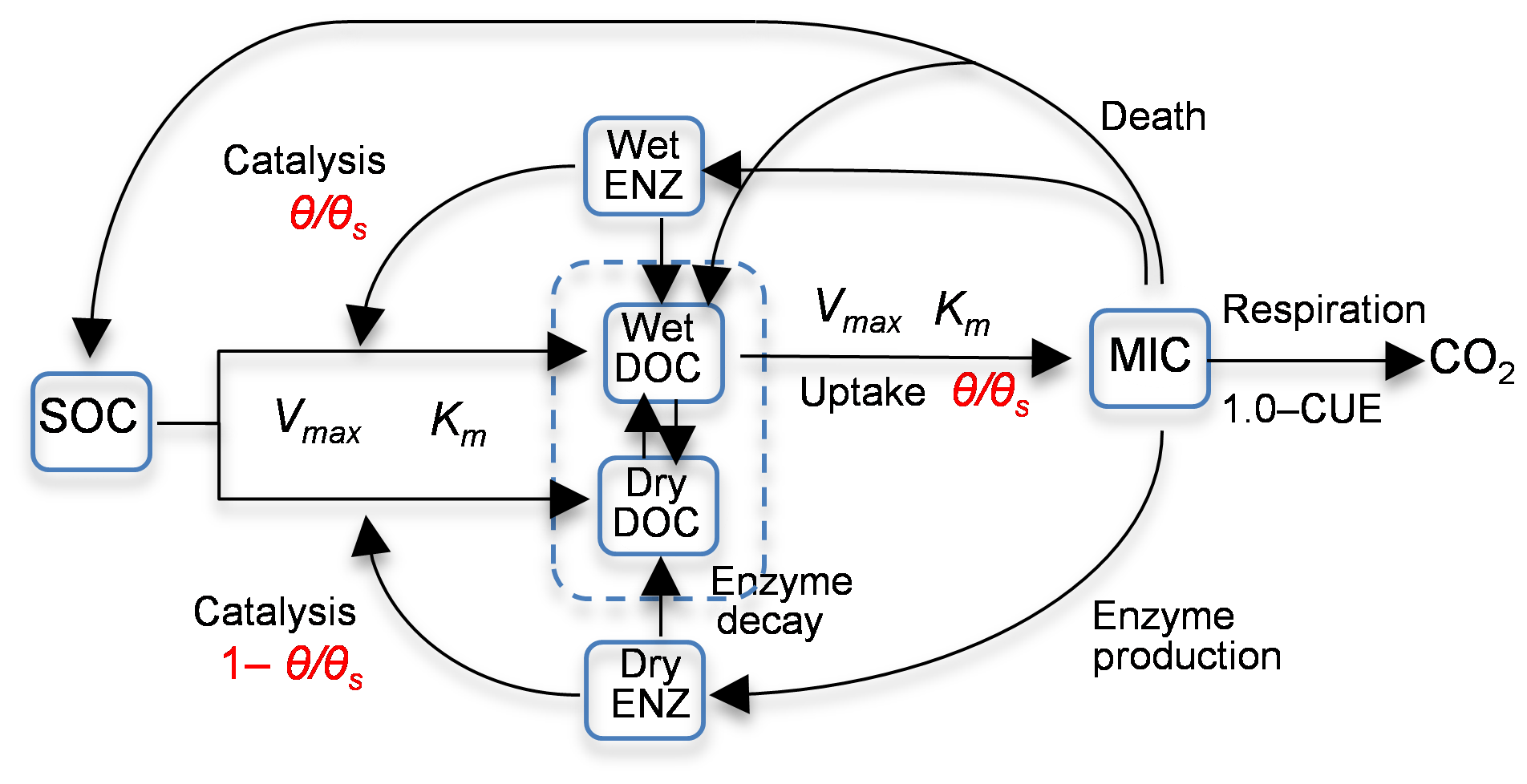
Figure 1 Diagram of model 6C representing the processes of (1) degradation of soil organic carbon (SOC) to dissolved organic carbon (DOC) through the catalysis of enzymes (ENZ) produced by microbes (MIC), (2) MIC uptake of DOC, and (3) microbial (MIC) respiration to produce CO₂ (CUE is the carbon use efficiency). SOC degradation and microbial uptake rates are controlled by water saturation (θ∕θ_s). The DOC and ENZ pools are split into two sub-pools, one for the wet zone and the other for the dry zone of the soil pore space. Microbial uptake of DOC only occurs in the wet zone, and the uptake rate is linearly related to θ∕θ_s. Catalysis through ENZ in the wet zone is proportional to θ∕θ_s, whereas that in the dry zone is proportional to $\mathrm{1}-\mathit{\theta }/{\mathit{\theta }}_{\mathrm{s}}$. V_max (s⁻¹) is the maximum rate, and K_m is the half-saturation concentration.

In addition to using the new rate equations, models 5C and 6C have more carbon pools. In model 5C, DOC is split into two sub-pools for the wet zone and the dry zone of soil pores, and only the wet DOC is used by MIC, as shown in Fig. 1. The moisture-controlled microbial uptake rate becomes

$$\begin{array}{ll}{\displaystyle }& {\displaystyle }{V}_{\mathrm{uptake}}=V_{max\mathrm{\_}\mathrm{up}}{C}_{\mathrm{MIC}}\\ \text{(18)}& {\displaystyle }& {\displaystyle }{\displaystyle \frac{C_{\mathrm{DOC}\mathrm{\_}\mathrm{W}}}{K_{m\mathit{\_}\mathrm{up}}+C_{\mathrm{DOC}\mathrm{\_}\mathrm{W}}}}{\displaystyle \frac{C_{{\mathrm{O}}_{\mathrm{2}}}}{K_{m\mathit{\_}\mathrm{up}{\mathrm{O}}_{\mathrm{2}}}+C_{{\mathrm{O}}_{\mathrm{2}}}}}\left({\displaystyle \frac{\mathit{\theta }}{{\mathit{\theta }}_{\mathrm{s}}}}\right),\end{array}$$

where C_{DOC_W} (g C m⁻³) is the DOC pool size in the wet soil pores. Model 6C is more complex in that ENZ is further split into two sub-pools for wet and dry pores, and both the wet and dry ENZ are subject to degradation, as shown in Fig. 1. The moisture-controlled SOC degradation rate becomes

$$\begin{array}{}\text{(19)}& {\displaystyle }{V}_{\mathrm{decom}}=V_{max}{C}_{\mathrm{ENZ}\mathrm{\_}\mathrm{W}}{\displaystyle \frac{C_{\mathrm{SOC}}}{K_m+C_{\mathrm{SOC}}}}\left({\displaystyle \frac{\mathit{\theta }}{{\mathit{\theta }}_{\mathrm{s}}}}\right)\end{array}$$

for the wet ENZ and

$$\begin{array}{}\text{(20)}& {\displaystyle }{V}_{\mathrm{decom}}=V_{max}{C}_{\mathrm{ENZ}\mathrm{\_}\mathrm{D}}{\displaystyle \frac{C_{\mathrm{SOC}}}{K_m+C_{\mathrm{SOC}}}}\left(\mathrm{1}-{\displaystyle \frac{\mathit{\theta }}{{\mathit{\theta }}_{\mathrm{s}}}}\right){\mathit{\epsilon }}_{\mathrm{D}}\end{array}$$

for the dry ENZ, where C_{ENZ_W} (g C m⁻³) is the wet soil pores enzyme pool size, C_{ENZ_D} (g C m⁻³) is the enzyme pool size in the dry soil pores, and ε_D is the catalysis efficiency of the dry zone enzyme.

Due to considering the moisture control and adding more soil pools, model 5C is expected to be significantly better than model 4C for simulating the Birch effect. As the accumulated ENZ in dry soil is secondary, model 6C is expected to be slightly better than model 5C. In terms of model structural error, model 4C has the largest model structure error, model 5C has significantly less model structure error, and model 6C has the smallest model structural error. In other words, model 6C has the highest model fidelity (i.e., lowest model discrepancy) among the three models. As shown below, the degree of model structural error is reflected in the process of Bayesian inference and verified by the cross-validation.

2.4 Observations and parameter estimation

Figure 2 plots the time series of 17 016 observations of soil moisture and CO₂ efflux used in this study. The observations were obtained during the entire year of 2007, covering a long period of dry season prior to the monsoon and episodic rainfall events during the monsoon. The first two-thirds of this dataset are used for the Bayesian inference, and the last third is used for cross-validation. The inference and cross-validation periods have both dry and wet periods, as shown in Fig. 2. The observation site is located within the Santa Rita Experimental Range (SRER; 31.8214^∘ N, 110.8661^∘ W, elevation 1116 m) outside of Tucson, Arizona (Barron-Gafford et al., 2011; Scott et al., 2009). This savanna site was covered by 22 % perennial grass, forbs, and subshrubs and 35 % mesquite. The soils are uniformly comprised of Comoro loamy sand (77.6 % sand, 11.0 % clay, and 11.4 % silt). The half-hourly atmospheric forcing data were collected from measurements via an eddy covariance tower (Scott et al., 2009). This includes downward shortwave radiation, longwave radiation, precipitation, wind, air temperature, humidity, and pressure. The volumetric CO₂ concentration was measured at a half-hourly intervals using compact probes. The CO₂ efflux was estimated from the gradient of the CO₂ concentration measured at two depths (2 and 10 cm) using Fick's first law of diffusion, and the estimates were validated against measurements from a portable CO₂ gas analyzer.

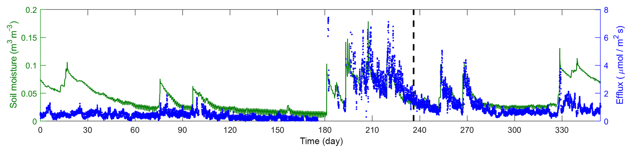
Figure 2 Time series of soil moisture and efflux observations. The dashed line marks the divide of the dataset into calibration and validation periods.

The parameters estimated in this study include the parameters of the soil respiration models (4C–6C) and the parameters of the data models described in Sect. 2.1. The estimated parameters of models 4C and 5C include the microbial carbon use efficiency (CUE) (g g⁻¹), enzyme production rate, k_e (g m⁻³ s⁻¹), microbial turnover rate, τ_m (1 s⁻¹), and enzyme turnover rate τ_e (1 s⁻¹). Uniform distributions are used as the prior in the Bayesian inference, and the ranges of the four parameters are 0.2–1.00, $\mathrm{1}\times {\mathrm{10}}^{-\mathrm{12}}$–$\mathrm{1}\times {\mathrm{10}}^{-\mathrm{7}}$, $\mathrm{1}\times {\mathrm{10}}^{-\mathrm{12}}$–$\mathrm{1}\times {\mathrm{10}}^{-\mathrm{5}}$, and $\mathrm{1}\times {\mathrm{10}}^{-\mathrm{11}}$–$\mathrm{1}\times {\mathrm{10}}^{-\mathrm{6}}$, respectively. The values of other parameters are fixed at the values used in Allison et al. (2010). Model 6C has two more parameters, and they are the catalysis efficiency ε_D (–) and the turnover rate of the dry-zone enzymes τ_en (1 s⁻¹). The priors of the two parameters are uniform distributions with the ranges of 0.2–0.8 and $\mathrm{1}\times {\mathrm{10}}^{-\mathrm{12}}$–$\mathrm{1}\times {\mathrm{10}}^{-\mathrm{8}}$, respectively.

The DREAM-based MCMC simulation is conducted for a total of 24 cases, the combinations of eight data models and three soil respiration models. For each case, the parameter distributions are obtained after drawing a total of 5×10⁵ samples using five Markov chains. The Gelman and Rubin (1992) R statistic is used for the convergence diagnostic, and it approaches 1 in less than 40 000 samples. The initial 50 % of the samples are discarded during the burn-in period.

2.5 Metrics for evaluating predictive performance

Three criteria are used to evaluate the predictive performance of the soil respiration models and data models: the central mean tendency, the dispersion, and the reliability. Each criterion is measured by a single metric. In addition, a newly defined metric by Elshall et al. (2018) is also used to simultaneously measure the three criteria.

The central mean tendency is measured in this study using the Nash–Sutcliffe model efficiency (NSME) coefficient (Nash and Sutcliffe, 1970),

$$\begin{array}{}\text{(21)}& {\displaystyle }\text{NSME}=\mathrm{1}-\sum _{i=\mathrm{1}}^n{\left(d_i-\stackrel{\mathrm{‾}}{{\mathit{Y}}_i}\right)}^{\mathrm{2}}/\sum _{i=\mathrm{1}}^n{\left(d_i-\stackrel{\mathrm{‾}}{\mathit{d}}\right)}^{\mathrm{2}},\end{array}$$

where n is the number of cross-validation data, d_i is the ith data, $\stackrel{\mathrm{‾}}{\mathit{d}}$ is the mean of the data, and $\stackrel{\mathrm{‾}}{{\mathit{Y}}_i}$ is the mean of the prediction ensemble, Y_i, for d_i. The NSME ranges from −∞ to 1, with NSME =1 corresponding to a perfect match between data and mean prediction, i.e., the ensemble is centered on the data. NSME =0 indicates that the model predictions are only as accurate as the mean of the data, whereas an efficiency NSME <1 indicates that the mean of data is a better prediction than the mean prediction.

In addition to the central mean tendency, it is also desirable that the ensemble is precise, with small dispersion, and reliable to cover all of the data. This study uses a nonparametric metric for dispersion, which is the sharpness of a prediction interval (e.g., M. W. Smith et al., 2010):

$$\begin{array}{}\text{(22)}& {\displaystyle }\text{Sharpness}=\mathrm{1}/n{\sum }_{i=\mathrm{1}}^n\left[\text{Max}\left({\mathit{Y}}_i\right)-\text{Min}\left({\mathit{Y}}_i\right)\right],\end{array}$$

where Y_i is the prediction ensemble within the 95 % prediction interval, the Bayesian credible interval, not the confidence interval used in nonlinear regression (Lu et al., 2013). Smaller sharpness values indicate better prediction precision. Reliability is measured using predictive coverage (e.g., Hoeting et al., 1999), which is the percentage of data contained in the prediction interval. Larger predictive coverage values are preferred.

To account for the trade-off between the three metrics, Elshall et al. (2018) defined relative model score (RMS) that simultaneously measures all three criteria. Scoring rules are commonly used in hydrology to assess predictive performance (e.g., Weijs et al., 2010; Westerberg et al., 2011). The RMS is used in this study to measure the relative predictive performance of the combinations of soil respiration models and data models. For combination M_j, RMS is defined as

$$\begin{array}{}\text{(23)}& {\displaystyle }\text{RMS}\left(M_j\right)=\sum _{i=\mathrm{1}}^n{\displaystyle \frac{p\left(d_i|{\mathit{Y}}_{ij},M_j\right)}{\sum _{j=\mathrm{1}}^{m}p\left(d_i|{\mathit{Y}}_{ij},M_j\right)}}\times \mathrm{100},\end{array}$$

where m is the number of combinations; the ensemble prediction Y_ij is similar to Y_i above with index i over time and index j specific to the jth combination. The density function p(d_i|Y_ij) can be evaluated by first obtaining the density function p(Y_ij) of the ensemble prediction Y_ij (e.g., by using the kernel density function) and then evaluating p(d_i|Y_ij) using interpolation methods based on the intersection of Y_ij and d_i. More details about evaluating RMS can be found in Elshall et al. (2018). This evaluation is based purely on the model predictions, and does not involve any assumptions on the models, their parameters, or their likelihood functions. Larger RMS values indicate better overall predictive performance. A figure displaying our workflow scheme is presented in the Supplement.

3 Results of Bayesian inverse modeling

This section analyzes the residuals of the best realization (with the highest likelihood value) of the MCMC simulation to understand whether the assumptions of the eight data models hold. The impacts of the data models on the posterior parameter distributions are also analyzed.

Figure 3 Residual analysis of the best realization (among multiple MCMC realizations) for model 6C using the (a–c) SLS and (d–f) WSEP-AC data models.

3.1 Residual characterization

Figure 3 shows residual plots for model 6C based on the SLS and WSEP-AC data models. SLS is the simplest data model with the assumptions of homoscedastic, independent, and Gaussian residuals, and WSEP-AC is the most complex model without the assumptions. Model 6C is the most complex model and also the best model as ranked by Zhang et al. (2014) using Bayesian model selection. The variable a_t, plotted in Fig. 3a–c and Fig. 3d–f, is defined in Eqs. (2) and (11), respectively. Figure 3a–c show that all three residual assumptions are violated when SLS is used, as (i) the residual variance is not constant, but increases as a function of the simulated CO₂ efflux (Fig. 3a); (ii) the autocorrelation function at most lags is beyond the 95 % confidence interval (Fig. 3b); and (iii) the standard normal density function cannot adequately characterize the residuals (Fig. 3c). Figure 3d–f show that, after relaxing the three assumptions, the processed residuals, a_t, can be well characterized by WSEP-AC. Figure 3d shows that, after normalizing ε_t with the linear variance (${\mathit{\sigma }}_t=\mathrm{0.034}+\mathrm{0.099}{E}_t$), the variation of the variance of a_t becomes significantly smaller, although the variance is still not constant. Figure 3e shows that, after removing a first-order autoregressive model from ε_t, a_t becomes less correlated, although the correlation is not fully removed. The two coefficients of the autoregressive model are ϕ₁=0.989 and ${\mathit{\varphi }}_{\mathrm{2}}=\mathrm{4.5}\times {\mathrm{10}}^{-\mathrm{6}}$; the small value of ϕ₂ indicates that there is no need to attempt an autoregressive model of higher order. Figure 3f shows that a_t follows the SEP distribution with the estimated skewness coefficient of ξ=0.933 and kurtosis coefficient of β=0.998. As a summary, Fig. 3 shows that it is important to examine the residuals and to determine whether the selected data model is adequate for characterizing the residuals. While WSEP-AC still cannot perfectly characterize ε_t, it is significantly better than SLS.

Figure 4 Residual quantile–quantile (Q–Q) plots of the best realization (among multiple MCMC realizations) for the three soil respiration models and eight data models.

Although the Gaussian assumption used in SLS is violated for model 6C (Fig. 3c), this is not generally the case for other data models and soil respiration models. This is shown in Fig. 4, which presents the quantile–quantile (Q–Q) plot for the eight data models and the three soil respiration models. For SLS, WLS, SLS-AC, and WLS-AC, the theoretical quantiles are based on the standard normal distribution, N(0, 1); for SEP, WSEP, SEP-AC, and WSEP-AC, the theoretical quantiles are based on the standard skew exponential power distribution, $\text{SEP}(\mathrm{0},\mathrm{1},\mathrm{1},\mathrm{0})$. If the residuals follow the assumed standard distributions, the Q–Q plots fall on the 1:1 lines, marked as the theoretical lines in Fig. 4. If the residuals are Gaussian or SEP but not standard, the Q–Q plots fall on a straight line but not on the 1:1 line. Figure 4a and e show that, for all of the soil respiration models, the Q–Q plots of SLS and SEP deviate significantly from the theoretical lines and exhibit fat-tail behaviors, which are an indication of outliers (Thyer et al., 2009). The deviation is reduced after accounting for autocorrelation in SLS-AC and SEP-AC, as shown in Fig. 4c and g. It is interesting to observe from the two figures that the Q–Q plots of the three models are visually almost identical. The deviation is almost fully removed after accounting for heteroscedasticity in WLS and WSEP in that their corresponding Q–Q plots fall on the 1:1 lines, especially for models 5C and 6C (as shown in Fig. 4b and f). However, the Q–Q plots start deviating from the 1:1 lines as shown in Fig. 4d and h, after accounting for both heteroscedasticity and autocorrelation in WLS-AC and WSEP-AC. In summary, Fig. 4 shows that, for the numerical example of this study, either the Gaussian or the SEP distribution is valid if heteroscedasticity is accounted for in the data models. However, accounting for autocorrelation in the data models does not help improve the characterization of the residual distributions.

3.2 Posterior parameter distributions

While Figs. 3 and 4 help understand the validity of the three assumptions used in the data models, the impacts of the data models on estimating model parameter distributions must be evaluated separately. This section discusses the impact of the data model selection on parameter estimation with the objective of understanding whether the incorrect specification of the data model necessarily leads to biased parameter estimates. Such assessment is not a trivial task for two main reasons. First, microbial soil respiration models aggregate complex natural processes and spatial details into simpler conceptual representations. As a result, several model parameters are effective values of several complex natural processes that cannot actually be measured in the field, as discussed by Vrugt et al. (2013). Second, even for model parameters that can be measured in the field, as the model structure is imperfect, calibrated parameter values are sometimes beyond their physically reasonable range, as discussed by Pappenberger and Beven (2006). This is often undesirable, if we seek to make the models more mechanistically descriptive.

We focus our discussion on the carbon use efficiency (CUE) for microbial growth due to two reasons: (1) the CUE is a fundamental parameter in microbial soil respiration models, and (2) a physically reasonable range can estimated for the CUE. The concept of microbial CUE (Allison et al., 2010; Bradford et al., 2008; Manzoni et al., 2012; Wieder et al., 2013) has been used to present fundamental microbial processes in recent microbial enzyme models (Allison et al., 2010; German et al., 2011; Schimel and Weintraub, 2003; Wang et al., 2013). The microbial CUE, which is marked between MIC and CO₂ in Fig. 1, controls microbial growth, enzyme production, and microbial respiration. A physically reasonable range of the CUE can be estimated from the physical viewpoint (Tang and Riley, 2014). Sinsabaugh et al. (2013) showed that the thermodynamic calculations support a maximum CUE of 0.60 and that previous studies that estimate CUE in terrestrial systems report a mean value of 0.55. Theoretically, there is no lower limit for the CUE as it can approach zero, and CUE <0.1 has been reported for terrestrial ecosystems (e.g., Fernández-Martínez et al., 2014) and used in modeling studies (Li et al., 2014). Note that, for inverse modeling with MCMC sampling, we did not assume a CUE maximum value of 0.6. In other words, for parameter estimation and predictive performance we did not impose the constraint that the CUE is less than 0.6. We merely use this CUE maximum value of 0.6 to evaluate whether the posterior CUE parameter samples obtained using different data models and different soil respiration models are within the physically reasonable range of 0–0.6.

Figure 5 Marginal posterior parameter density of carbon use efficiency (CUE) for the three soil respiration models and eight data models. The yellow shaded areas represent the reasonable physical range of CUE (0–0.6).

Figure 5 plots the CUE posterior marginal density of the three soil respiration models obtained using the eight data models. The physical range between zero and 0.6 is marked in yellow. Figure 5 shows that the CUE posterior parameter distribution of model 6C (obtained using the data models) that does not account for autocorrelation is within the physically reasonable range. For models 4C and 5C, the posterior parameter samples are outside the range for six data models. For model 4C, the posterior parameters are only within the physical range for the SEP and WSEP data models; for model 5C, the two data models are WLS and WSEP. It is not surprising to find the posterior parameter distribution of models 4C and 5C, which have a certain degree of model structure error, to be outside of the physically plausible range. This can be attributed to two reasons. First, the model solution can be biased toward the missing processes in the model structure such as the additional carbon pool in both 4C and 5C or missing the explicit accounting for soil moisture in 4C. Second, biased parameter estimation can compensate for model structure inadequacy and other sources of discrepancy in both the physical models and the data models.

In addition, it is important to understand how accounting for autocorrelation, heteroscedasticity, and non-Gaussian residuals can affect the parameter estimation. First, it is observed in Fig. 5e–h that biased parameter estimates are outside of the physically reasonable range when autocorrelation is explicitly accounted for. This may suggest again that accounting for heteroscedasticity is desirable but accounting for autocorrelation is not. A possible reason is that filtering autocorrelation may reduce the residual space such that the transformed residual space cannot correspond to the parameter space of the models. In other words, parameter information may be lost due to filtering out autocorrelation. However, it is not fully understood why this does not occur for model 6C under data model SLS-AC (Fig. 5e), and more research is warranted. Second, unlike accounting for autocorrelation, accounting for heteroscedasticity alone (i.e., WLS and WSEP) only amplifies or reduces the variance without affecting the structure of the residual space. Figure 5c and d show that accounting for heteroscedasticity (i.e., WLS and WSEP) tends to improve the parameter estimation in comparison with the homoscedastic data models (i.e., SLS and SEP) shown in Fig. 5a and b. Finally, with respect to non-Gaussian residuals, Schoups and Vrugt (2010) suggested that, compared to Gaussian PDF, the peaked PDF of the SEP with a longer tail is useful for making the parameter inference robust against outliers. To a certain degree, this can be substantiated by the results in Fig. 5a–d, in that SEP and WSEP provide more favorable parameter estimates than SLS and WLS.

Finally, Fig. 5a shows that the posterior parameter distributions of SLS are very narrow for the three soil respiration models. The narrow distributions can be attributed to several reasons. As a SEP distribution can have longer tails than a Gaussian distribution, this can further increase the sample's acceptance ratio from tails resulting in a wider distribution (Fig. 5b). In addition, accounting for heteroscedasticity will result in a wider posterior parameter distribution (Fig. 5c) due to accepting higher variances at peak effluxes. Moreover, filtering correlation (Fig. 5e–h) increases the entropy, and leads to wider distributions.

4 Results of predictive performance

Based on the last one-third of the CO₂ efflux observations, a cross-validation test was conducted for the combinations of three soil respiration models and eight data models. For the cross-validation period, the predictive performance is examined using the four statistical metrics defined in Sect. 2.5. The metrics are also calculated for the calibration period. This is not to perform Bayesian model selection given the calibration data, but to better understand the impact of data models on predictive performance of the three soil respiration models. For each calibration and each cross-validation dataset, a prediction ensemble is generated from the two perspectives: parametric uncertainty only, and total uncertainty. These two perspectives are presented in Sect. 4.1 and 4.2, respectively.

4.1 Predictive performance with parametric uncertainty of soil respiration model

In this section the ensemble is generated by running the soil respiration models with the posterior samples (obtained from the Bayesian inference) of the physical model parameters. In other words, the ensemble addresses parametric uncertainty of the soil respiration models only. Considering the relative contribution of parametric uncertainty only will provide insights for modeling approaches that attempt to segregate various sources of uncertainty (e.g., Thyer et al., 2009; Tsai and Elshall, 2013). The four statistics above (i.e., NSME, sharpness, coverage, and RMS) are calculated for the three soil respiration models and the eight data models. Taking the SLS and WSEP-AC data models as examples, Fig. 6 plots the data (for the calibration and cross-validation periods separately) along with the mean and 95 % credible intervals of the prediction ensemble for the three models.

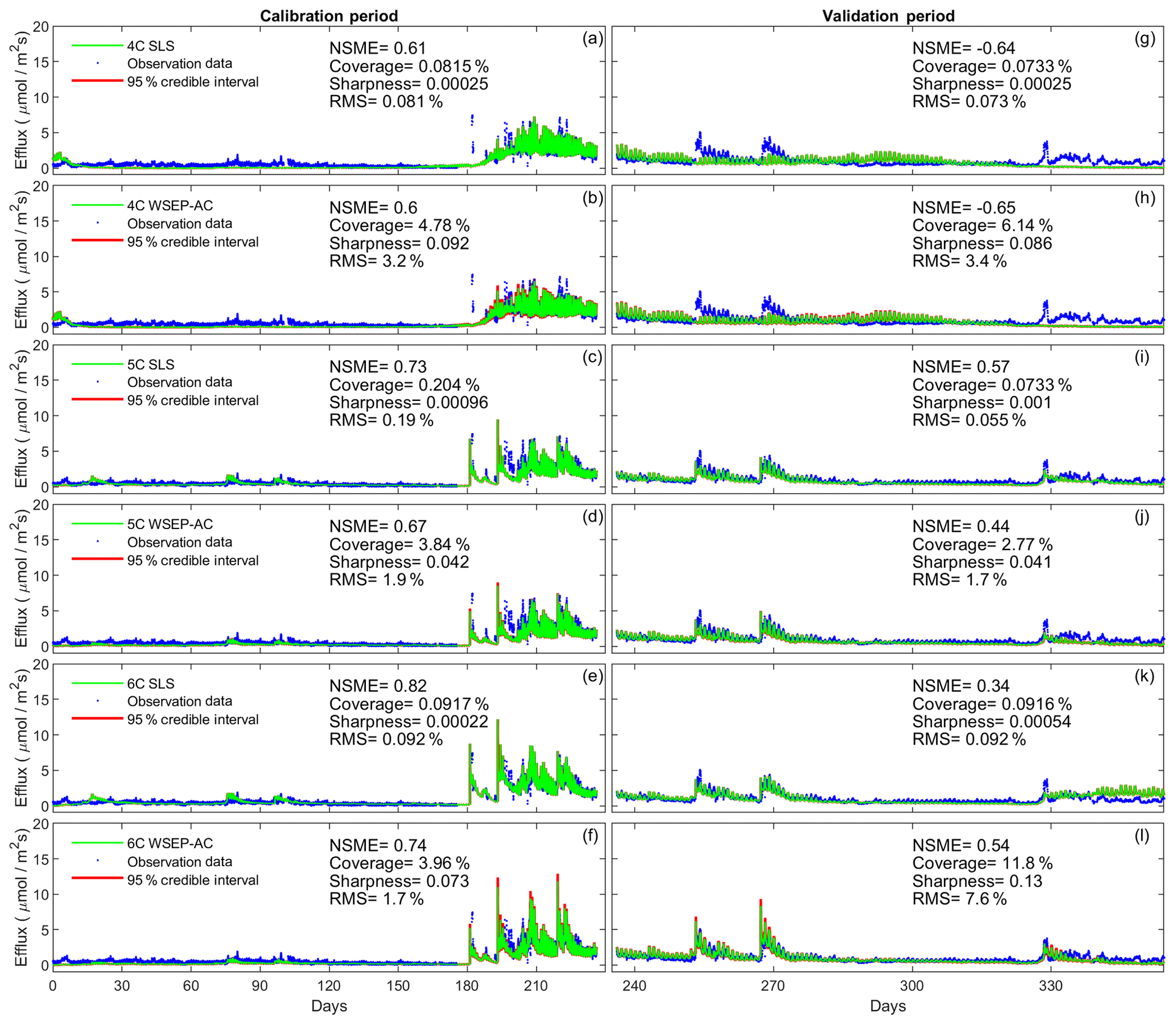
Figure 6 Observation data (blue dots), mean prediction (green line), and 95 % credible intervals (red line) of prediction ensembles for (a–f) the calibration period and (g–l) the validation period. The plots are for the three soil respiration models using the SLS and WSEP-AC data models. The prediction ensembles are generated to consider parametric uncertainty of the soil respiration models only. The model prediction accuracy, reliability, dispersion and overall predictive performance are measured by the Nash–Sutcliffe model efficiency (NSME), the predictive coverage metric (“Coverage”), the sharpness metric (“Sharpness”) and the relative model score (RMS), respectively.

Figure 6 shows that the data models affect model simulations for all of the models. The statistics, especially the RMS, indicate that WSEP-AC has better predictive performance than SLS. This is most visually obvious for model 6C during the cross-validation period after 330 d, as the prediction ensemble of SLS (Fig. 6k) cannot cover the observations, whereas the prediction ensemble of WSEP-AC can (Fig. 6l). This conclusion that WSEP-AC outperforms SLS agrees with the conclusion drawn from Figs. 3 and 4.

Figure 7 plots the four statistics for all of the soil respiration models and data models. Figure 7a and b show the predictive performance with respect to the central mean tendency measured by the NSME for both the calibration and cross-validation periods, respectively. The results indicate that, under all data models, the low-fidelity model 4C over-fits the data and results in biased predictions, in that the NSME values become significantly worse (e.g., from 0.6 to −0.6) from the calibration to the cross-validation period. This is confirmed by the visual inspection of Fig. 6a and g for data model SLS and of Fig. 6b and h for data model WSEP-AC. For models 5C and 6C, the NSME values vary with the data models; the central mean accuracy is the worst for SLS-AC that only considers autocorrelation (Fig. 6b).

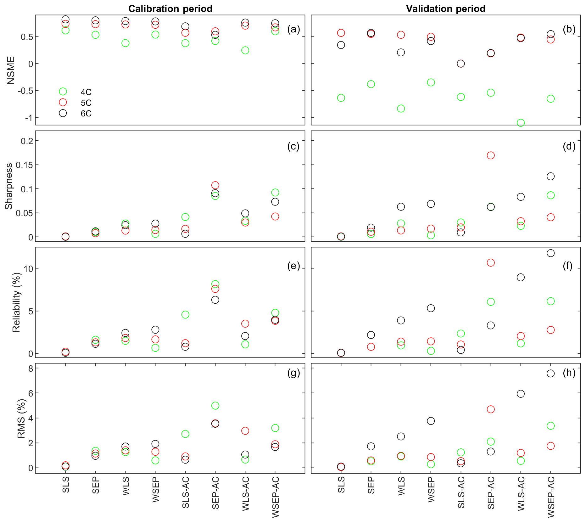
Figure 7 (a, b) Nash–Sutcliffe model efficiency (NSME), (c, d) sharpness, (e, f) predictive coverage, and (g, h) relative model score for measuring predictive performance of the three soil respiration models and the eight data models during the calibration and cross-validation periods. The statistics are evaluated from the prediction ensembles generated to consider parametric uncertainty of the soil respiration models only.

With respect to the parametric uncertainty estimation, Fig. 7c and d show that sharpness generally increases when the three assumptions in the data models are gradually relaxed from SLS to WSEP-AC. This is even more obvious during the validation period. Given that the prediction ensemble does not center on the data, the increasing sharpness is desirable as it improves reliability. This is confirmed by the reliability plots in Fig. 7e and f. The exceptions are once again for SLS-AC and SEP-AC that generally have the lowest coverage.

With respect to the overall predictive performance measured by the RMS, the same variation pattern and exception are also observed in the RMS plots in Fig. 7g and h. This is not surprising because the RMS is the metric that can be used to measure all three criteria (central mean tendency, sharpness, and reliability). As the prediction ensemble is not centered on the data, the sharpness and reliability are the decisive factors for evaluating the predictive performance.

In summary, while it is necessary to account for heteroscedasticity in a data model, caution is needed when accounting for autocorrelation in the manner described in Sect. 2.1. In addition, after comparing the RMS values of the residuals using the Gaussian and SEP distributions, the conclusion is that the SEP distribution outperforms the Gaussian distribution with respect to predictive performance. Finally, uncertainty underestimation is evidenced by the very small predictive coverage. The underestimation of uncertainty for all of the physical models with all of the data model is not unexpected because only parametric uncertainty is considered in this study. Considering the overall predictive uncertainty is the subject of the next section.

4.2 Predictive performance with total uncertainty

The simulated output Y(θ_p) is generally not equal to the observed output d, and we have a residual term ε due to measurement, input, and model structure errors such that $\mathit{d}=\mathit{Y}\left({\mathit{\theta }}_p\right)+\mathit{\epsilon }$. Accounting for the error term ε can be undertaken by separating various error terms. For example, in Sect. 4.1 we obtained uncertainty due to the physical model parameters. Accounting for other sources of uncertainty can be carried out using a single model approach (e.g., Thyer et al., 2009) or a multi-model approach (e.g., Tsai and Elshall, 2013). Alternatively, we can quantify the uncertainty based on total residuals that separates out parametric uncertainty, so the residual error includes errors in measurements, model inputs, and model structures (e.g., Thyer et al., 2009; Schoups and Vrugt, 2010). This lumped approach is based on sampling the residuals model ε(θ_ε) with parameters θ_ε. SLS has one fixed parameter, the constant variance, and other data models have two to six parameters. Thus, in this section the prediction ensemble addresses parametric uncertainty of not only the soil respiration models but also the data models. When generating the prediction ensemble in the procedure described by Schoups and Vrugt (2010), an ensemble of residuals is first generated by running the data models with posterior samples of the data model parameters for the positive carbon efflux domain; the residual ensemble is then added to the prediction ensemble generated in Sect. 4.1.

We start by undertaking a visual assessment of the predictive performance. Figure 8 is similar to Fig. 6 with the exception that Fig. 8 considers the overall predictive uncertainty (i.e., parametric and output uncertainty), whereas Fig. 6 only considers the parametric uncertainty. Figure 8 reveals a practical observation about accounting for the overall uncertainty using the lumped approach of sampling the data models. For example, Fig. 8b shows that, despite the wide prediction interval of model 4C, the model with significant model structure error cannot capture the birch pulse around day 180. It indicates that properly using a data model for model residuals cannot compensate for significant model structure error.

Figure 8 Observation data (blue dots), mean prediction (green line), and 95 % credible intervals (red line) of prediction ensembles for (a–f) the calibration period and (g–l) the validation period. The plots are for the three soil respiration models using the SLS and WSEP-AC data models. The prediction ensembles are generated to consider parametric uncertainty of not only the soil respiration models but also the data models. The model prediction accuracy, reliability, dispersion and overall predictive performance are measured by the Nash–Sutcliffe model efficiency (NSME), the predictive coverage metric (“Coverage”), the sharpness metric (“Sharpness”) and the relative model score (RMS), respectively.

Figure 9 plots the four statistics (NSME, sharpness, predictive coverage, and RMS) of the three soil respiration models under the eight data models to assess the predictive performance. With respect to the central mean tendency, the NSME values in Fig. 9a and b are visually the same as those in Fig. 7a and b, indicating that the central mean accuracy under parametric uncertainty is the same as that under predictive uncertainty.

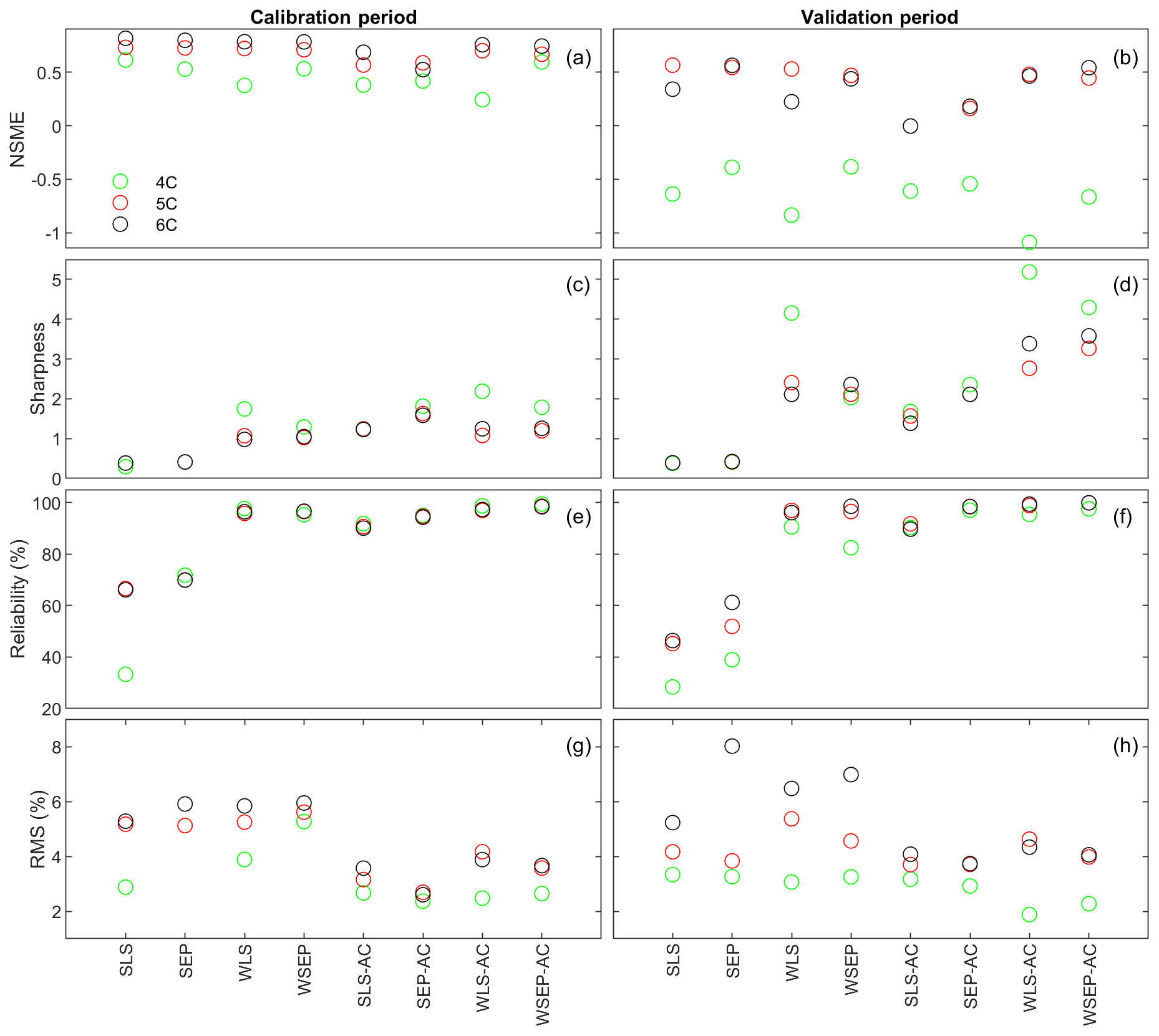
Figure 9 (a, b) Nash–Sutcliffe model efficiency (NSME), (c, d) sharpness, (e, f) predictive coverage, and (g, h) relative model score for measuring predictive performance of the three soil respiration models and the eight data models during the calibration and cross-validation periods. The statistics are evaluated from the prediction ensembles generated to consider parametric uncertainty of not only the soil respiration models but also the data models.

With respect to uncertainty, the values of sharpness and predictive coverage increase substantially (Fig. 9c–f). In particular, Fig. 9e and f show that, except for SLS and SEP, the predictive coverage of the rest of the six data models are close to 100 % for all three soil respiration models, indicating that the prediction intervals cover almost all of the data. This is demonstrated in Fig. 6 for WSEP-AC. Similar to Figs. 7c and d, Figs. 9c and d also show a general pattern where the sharpness increases when the three assumptions in the data models are gradually relaxed from SLS to WSEP-AC. The data models that account for autocorrelation are still the exceptions.

With respect to the overall predictive performance, the RMS values are largely determined by the mean accuracy and sharpness as the predictive coverage is similar for different data models. Figure 9g and h of RMS show that the predictive performance of the four data models that account for autocorrelation is worse than that of the other four data models. This suggests again that one needs to be cautious when building autocorrelation into a data model. This is consistent with the finding of Evin et al. (2013, 2014) that accounting for autocorrelation before accounting for heteroscedasticity or jointly accounting for autocorrelation and heteroscedasticity can result in poor predictive performance. In summary, Fig. 9g and h show that accounting for heteroscedasticity in WLS and WSEP for both the calibration and prediction periods gives the best overall predictive performance, and accounting for autocorrelation without heteroscedasticity in SLS-AC and SEP-AC gives the worst overall predictive performance. Finally, for the three soil respiration models, RMS shows that model 4C has the worst predictive performance for both the calibration and cross-validation data. Generally speaking, the high-fidelity model 6C outperforms model 5C for both the calibration and cross-validation data, which justifies the complexity of model 6C.

To demonstrate the impacts of the data models on the predictive performance of the soil respiration models, Fig. 10 plots the model simulations and predictions given by model 6C during the calibration and cross-validation periods using all the eight data models. Figure 10 is used to investigate predictive performance characteristics of the different data models. By examining the predictive performance of model 6C, specific predictive performance patterns can be identified. Figure 10a–d show that SLS and SEP have similar predictive performance with SEP generally having better predictive performance especially during the validation period. Not accounting for heteroscedasticity will underestimate the predication uncertainty (Fig. 10b, d). This is mainly because the variance of the efflux residuals increases with the magnitude of the carbon effluxes (Fig. 3a); thus, assuming constant variance is not representative. Accordingly, accounting for heteroscedasticity using WLS (Fig. 10e) or WSEP (Fig. 10h) will make the predictions more sensitive to peak carbon effluxes. This will generally improve the predictive coverage on the expense of sharpness and the central mean tendency. While WLS and WSEP have similar predictive performance, WSEP has better central mean tendency and overall predictive performance than WLS. Figure 10i–l show that accounting for autocorrelation using SLS-AC and SEP-AC results in wider uncertainty bands and insensitivity to peak carbon effluxes compared with SLS and SEP (Fig. 10a–d), which may be due to the reduction in the information content of the residuals. This results in the deterioration of the sharpness, the central mean tendency, and the capturing of peak carbon fluxes, especially during the validation period. Figure 10m–p show that accounting for both heteroscedasticity and autocorrelation using WLS-AC and WSEP-AC makes the inference robust against peak carbon effluxes. However, due to the loss of information content, the uncertainty bands are still wider, and the uncertainty becomes overestimated especially during validation period compared with WLS and WSEP (Fig. 10e–h). The results of models 4C and 5C, which are not shown here, also display the same prediction patterns with respect to non-Gaussian residuals, heteroscedasticity, and autocorrelation.

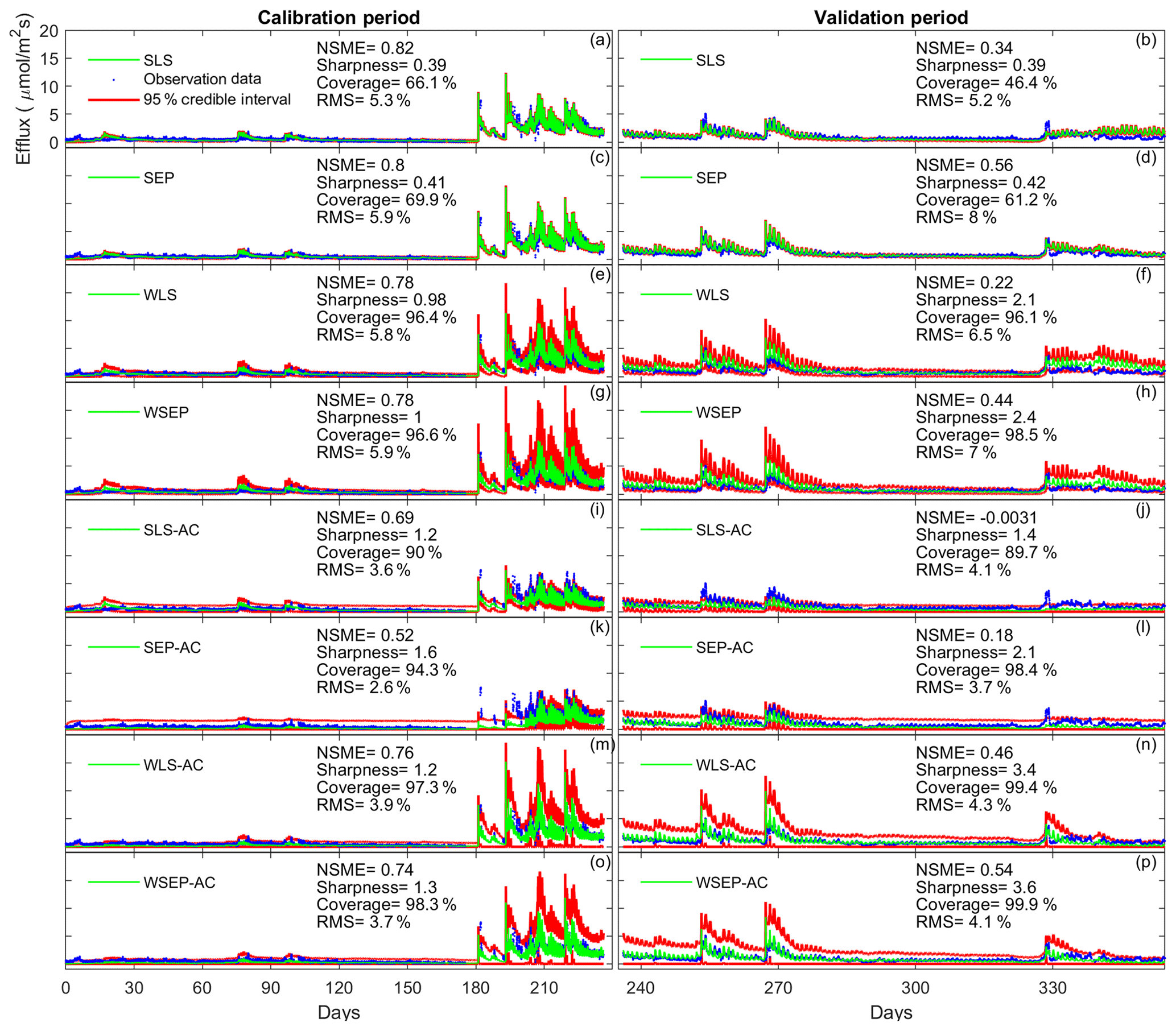
Figure 10 Observation data (blue dots), mean prediction (green line), and 95 % credible intervals (red line) for 6C for the eight likelihood functions during the calibration period (a–h) and the validation period (i–p). The prediction ensembles are generated to consider parametric uncertainty of not only the soil respiration models but also the data models. The model prediction accuracy, reliability, dispersion and overall predictive performance are measured by the Nash–Sutcliffe model efficiency (NSME), the predictive coverage metric (“Coverage”), the sharpness metric (“Sharpness”) and the relative model score (RMS), respectively. For clarity, the y axis markers and label are only displayed for the first subplot and are the same for all subplots.

Finally, we observe in Fig. 10 that the data models that have good overall predictive performance as measured by RMS during the calibration period will maintain this good predictive performance during the validation period. For model 6C, the RMS values for the calibration and validation periods are very well correlated with a correlation coefficient of 0.92. However, we note that for models 4C and 5C the overall predictive performances during the calibration and validation periods are not as well correlated as for 6C, with correlation coefficients of 0.52 for model 4C and 0.61 for model 5C. This suggests that model 6C is more robust than 4C and 5C for forecasting and hindcasting.

4.3 Discussion on handling residual correlation

Accounting for autocorrelation can lead to biased parameter estimation (Fig. 5) and poor predictive performance (Fig. 10). Autocorrelated residuals may be attributed to model discrepancy, as shown in Lu et al. (2013). The most obvious solution to handle the autocorrelation is to reduce the autocorrelation by improving the soil respiration model. If model improvement is difficult for practical reasons, we can improve the data model to better characterize the autocorrelation. Addressing autocorrelation in a data model is challenging, as it involves several interlinked factors as follows:

1. Non-stationarity could be a reason for this problem. By drawing on similarity from surface hydrology, the study of Ammann et al. (2018) suggests that autocorrelated residuals might be attributed to non-stationarity due to wet–dry periods with half-hourly data. Accounting for non-stationarity due to wet–dry periods could better address the problem of autocorrelated residuals (Ammann et al., 2018; T. Smith et al., 2010).

2. The way that autocorrelation is implemented could have an impact. Autocorrelation could be directly applied to raw residuals (e.g., Li et al., 2015), to transformed residuals based on the covariance matrix of residuals L(e) (e.g., Lu et al., 2013), or to normalized residuals L(a) (e.g., Schoups and Vrugt, 2010; Evin et al., 2013). Note that “e” is a vector of transformed residuals, whereas “a” denotes a vector of independent and identically distributed random errors with a zero mean and unit standard deviation. The L(e) approach based on covariance matrix of residuals is generally limited to Gaussian data models (e.g., Lu et al., 2013), whereas the L(a) approach for normalized residuals can be readily adopted for non-Gaussian data models.

3. The autocorrelation model could have an impact. Using an autoregressive model is a popular technique to account for autocorrelated residuals. However, using an autoregressive model with either a joint inversion approach (e.g., this study and Schoups and Vrugt, 2010) or sequential approaches (e.g., Evin et al., 2013, 2014; Lu et al., 2013) removes correlation errors via a filter approach, which can lead to a loss of information content. As this may cause an overcorrection of prediction especially at surge events, Li et al. (2015) developed a restricted autoregressive model to overcome this adverse effect. Other autocorrelation models include the moving average model and the mixed autoregressive-moving averaging model (Chatfield, 2003).

4. Joint vs. sequential inversion for autocorrelation could have an impact. Sequential inversion approaches include two-step procedures (e.g., Evin et al., 2013, 2014; Lu et al., 2013) or the multi-step procedure (M. Li et al., 2016). These sequential approaches estimate the autoregressive parameters sequentially in a later step after estimating the physical model parameters and other data model parameters. Evin et al. (2013, 2014) used a sequential approach to avoid the interaction between the parameters of the heteroscedasticity model and the autocorrelation model. In addition, the autoregressive model parameters can be deterministically calculated as internal variables of the data model similar to Lu et al. (2013), and not as calibration parameters (e.g., Schoups and Vrugt, 2010; Evin et al., 2013, 2014). While the first step in the sequential approach would avoid the biased parameter estimation (Fig. 10a–d), the second step can still lead a poor predicative performance as we are essentially using a filter approach to remove residual correlation. To address this problem, M. Li et al. (2016) utilizes a multi-step procedure that is based on a Gaussian data model that uses restricted autoregressive model. Generally, the study by Ammann et al. (2018) states that joint inversion is still preferred, and that understanding the conditions under which accounting for autocorrelation can be achieved remains poorly understood.

5 Conclusions

In parameter estimation and prediction of soil carbon fluxes to the atmosphere, one often assumes that residuals, which include errors in observations, model inputs, parameter estimates, and model structures, are normally distributed, homoscedastic, and uncorrelated. We study these assumptions by calibrating three soil respiration models, which have varying degrees of model structure errors. We further explore eight data models that statistically characterize the residuals; we start with the standard least squares (SLS) and skew exponential power (SEP) data models that assume homoscedastic and non-correlated residuals. For these two distributions, we evaluate six other data models that account for heteroscedasticity (WLS and WSEP), autocorrelation (SLS-AC and SEP-AC), and joint inversion of heteroscedasticity and autocorrelation (WLS-AC and WSEP-AC). To our knowledge this is the first study that provides such a detailed analysis for soil reparation inverse modeling. We also use three soil respiration models with different degrees of model fidelity (i.e., model discrepancy) and model complexity (i.e., number of model parameters) to understand the impact of model discrepancy on the calibration results under different data models. We analyze the results with respect to (1) residual characterization, (2) parameter estimation, (3) predictive performance, and (4) impacts of model discrepancy. The main findings of this study are summarized as follows:

1. With respect to residual characterization, residual analysis results suggest that the common assumption of not accounting for heteroscedasticity and residual autocorrelation in the SLS and SEP data models results in the poor characterization of residuals. Explicitly accounting for heteroscedasticity in WLS and WSEP results in the significantly improved characterization of the residuals, and the improvement is larger than that obtained by accounting for both heteroscedasticity and autocorrelation in WSL-AC and WSEP-AC. Accounting for autocorrelation only in SLS-AC and SEP-AC does not significantly improve the characterization of the residuals.

2. With respect to parameter estimation, the impacts of the data models are evaluated by focusing on the carbon use efficiency (CUE), which is a central parameter in soil respiration modeling. Using SLS yields relatively reasonable posterior parameter distributions for the CUE , yet very narrow posteriors. The SLS-AC, SEP-AC, WLS-AC, and WSEP-AC data models that consider autocorrelation tend to yield CUE estimates that are physically unreasonable. We speculate that filtering residual correlation can affect the mapping of the model physics (as implicitly included in the residuals) into the parameter space, which might result in biased parameter estimates that are physically unreasonable.

3. With respect to predictive performance, it is measured by four statistical criteria: central mean tendency, sharpness, coverage, and relative model score for both the calibration and the cross-validation periods. Results show that accounting for autocorrelation in SLS-AC, SEP-AC, WLS-AC, and WSEP-AC reduces the predicative performance, such that the predictive performance is inferior to that of SLS in terms of the central mean tendency and overall predictive performance (measured by the relative model score), especially during the cross-validation period. Results also indicate that using the SEP distribution can potentially improve the predictive performance. The same is true for accounting for heteroscedasticity. Using the SEP distribution and accounting for heteroscedasticity (i.e., WSEP) can potentially improve the predictive performance.

4. With respect to the impact of model discrepancy, the high-fidelity model (6C) gives the best results with respect to parameter estimation and predictive performance. Model 6C generally maintains its superior performance under different data models. This justifies the complexity of model 6C relative to model 5C that has one less carbon pool. Model 4C, with the lowest fidelity, maintains its poor performance for different data models, because the model only has four carbon pools and lacks the explicit representation of soil moisture control.

Based on the empirical findings above, we conclude the following:

1. Not accounting for heteroscedasticity and autocorrelation using a Gaussian or non-Gaussian data model might not necessarily result in biased parameter estimates or biased predictions with respect to the central mean tendency, but will definitely underestimate uncertainty resulting in lower overall predictive performance.

2. Using a non-Gaussian data model can improve the parameter estimation and predictive performance with respect to the central mean tendency and the uncertainty quantification.

3. Accounting for heteroscedasticity improves the uncertainty estimation with respect to reliability at the cost of having a wider predictive interval.

4. This study confirms other empirical findings and theoretical analyses (Evin et al., 2013, 2014; Li et al., 2015; Ammann et al., 2018) which propose that separately accounting for autocorrelation or jointly accounting for autocorrelation and heteroscedasticity can be problematic. While the reasons remain poorly understood (Ammann et al., 2018), this might be attributed to non-stationarity due to wet–dry periods with half-hourly data (Ammann et al., 2018) or to the method of handling autocorrelation (e.g., Schoups and Vrugt, 2010; Evin et al., 2013, 2014; Lu et al., 2013; M. Li et al., 2015, 2016; Ammann et al., 2018). Further investigation to address autocorrelation in soil respiration modeling is warranted in a future study.

The above conclusions are subject to several limitations. First, the conclusions are specific to the soil respiration models developed and validated for semi-arid savannah landscapes. Performance variations across different soil respiration models with different levels of complexity are possible. Second, the conclusions are conditioned on data that were obtained at half-hourly intervals over a 1-year period. Different conclusions would be possible if the data were thinned to daily or weekly scales or data from longer observation periods were used. Third, our study investigates the effects of the residual assumptions of formal likelihood functions via direct conditioning of the residuals model parameters, yet this can also be undertaken using other approaches such as residuals transformation (Thiemann et al., 2001), autoregressive bias models (Del Giudice et al., 2013), approximate Bayesian computation (Sadegh and Vrugt, 2013), and data assimilation (Spaaks and Bouten, 2013). Comparing different methods for accounting for the residual assumptions are beyond the scope of this work. Fourth, this study focuses on formal Bayesian computation using formal likelihood functions, and comparison with other inference functions such as informal likelihood functions or approximate Bayesian computation is warranted in a future study.

Based on the aforementioned conclusions and limitations, we recommend beginning the calibration of soil respiration models with simple SLS or SEP likelihood function. If the residuals characterization is adequate (e.g., Scharnagl et al., 2011), then the underlying assumptions are met. Otherwise, the complexity of the data model can be increased until satisfactory results are obtained in terms of residuals characterization, posterior parameter estimation, and predictive performance. This is similar to the procedure given in Smith et al. (2015). Although the empirical findings of this study provide general guidelines for data model selection for soil respiration modeling, more comparative studies are needed to validate or refute the findings of this study.

Appendix A: Acronyms

4C	Four-carbon-pool model
5C	Five-carbon-pool model
6C	Six-carbon-pool model
CUE	Microbial carbon use efficiency
DOC	Dissolved organic carbon
ENZ	Enzymes
MCMC	Markov chain Monte Carlo
MIC	Microbial biomass
NSME	Nash–Sutcliffe model efficiency
PDF	Probability density function
RMS	Relative model score
SEP	Skew exponential power distribution
SEP-AC	Skew exponential power distribution with autocorrelation
SLS	Standard least square
SLS-AC	Standard least square with autocorrelation
SOC	Soil organic carbon
WLS	Weighted least squared
WLS-AC	Weighted least squared with autocorrelation
WSEP	Weighted skew exponential power distribution
WSEP-AC	Weighted skew exponential power distribution with autocorrelation