Towards end-to-end (E2E) modelling in a consistent NPZD-F modelling framework (ECOSMO E2E_v1.0): application to the North Sea and Baltic Sea

Coupled physical–biological models usually resolve only parts of the trophic food chain; hence, they run the risk of neglecting relevant ecosystem processes. Additionally, this imposes a closure term problem at the respective “ends” of the trophic levels considered. In this study, we aim to understand how the implementation of higher trophic levels in a nutrient–phytoplankton–zooplankton–detritus (NPZD) model affects the simulated response of the ecosystem using a consistent NPZD–fish modelling approach (ECOSMO E2E) in the combined North Sea–Baltic Sea system. Utilising this approach, we addressed the above-mentioned closure term problem in lower trophic ecosystem modelling at a very low computational cost; thus, we provide an efficient method that requires very little data to obtain spatially and temporally dynamic zooplankton mortality.

On the basis of the ECOSMO II coupled ecosystem model we implemented one functional group that represented fish and one group that represented macrobenthos in the 3-D model formulation. Both groups were linked to the lower trophic levels and to each other via predator–prey relationships, which allowed for the investigation of both bottom-up processes and top-down mechanisms in the trophic chain of the North Sea–Baltic Sea ecosystem. Model results for a 10-year-long simulation period (1980–1989) were analysed and discussed with respect to the observed patterns. To understand the impact of the newly implemented functional groups for the simulated ecosystem response, we compared the performance of the ECOSMO E2E to that of a respective truncated NPZD model (ECOSMO II) applied to the same time period. Additionally, we performed scenario tests to analyse the new role of the zooplankton mortality closure term in the truncated NPZD and the fish mortality term in the end-to-end model, which summarises the pressure imposed on the system by fisheries and mortality imposed by apex predators.

We found that the model-simulated macrobenthos and fish spatial and seasonal patterns agree well with current system understanding. Considering a dynamic fish component in the ecosystem model resulted in slightly improved model performance with respect to the representation of spatial and temporal variations in nutrients, changes in modelled plankton seasonality, and nutrient profiles. Model sensitivity scenarios showed that changes in the zooplankton mortality parameter are transferred up and down the trophic chain with little attenuation of the signal, whereas major changes in fish mortality and fish biomass cascade down the food chain.

1 Introduction

The majority of spatially resolved marine ecosystem models are dedicated to a specific part of the marine food web. These models can be differentiated into lower-trophic-level nutrient–phytoplankton–zooplankton models (so-called NPZ models or LTL models – e.g. Blackford et al., 2004; Daewel and Schrum, 2013; Maar et al., 2011; Schrum et al., 2006; Skogen et al., 2004) and, on the other end of the trophic chain, higher-trophic-level models (HTL models). The latter mainly simulate fish on the species level, including both single-species individual-based models (IBMs; e.g. Daewel et al., 2008; Megrey et al., 2007; Politikos et al., 2018; Vikebø et al., 2007) and multi-species models. Although some of these models are complex and already include many food web components such as OSMOSE (Shin and Cury, 2004, 2001) and ERSEM (Butenschön et al., 2016), the separation of trophic levels often constrains such models' ability to simulate and distinguish between major control mechanisms on marine ecosystems (Cury and Shannon, 2004). The difficulty of resolving trophic feedback mechanisms increases the uncertainties when modelling the impacts of external controls on the trophic food chain (e.g. Daewel et al., 2014; Peck et al., 2015).

In the last 10 to 15 years, major efforts have been made to link the different trophic levels together to cover the marine ecosystem from the lowest to the uppermost “end” (end-to-end: E2E) (Christensen and Walters, 2004; Fennel, 2009; Fulton, 2010; Heath, 2012; Shin et al., 2010; Travers et al., 2007; Watson et al., 2014). Although some models such as Atlantis (Fulton et al., 2005), StrathE2E (Heath, 2012), and Ecopath with Ecosim (EwE; Christensen and Walters, 2004) consider more trophic levels (from phytoplankton to marine mammals and birds and/or fisheries) consistently within the model formulation, the majority of approaches couple conceptually different model types – either “one-way”, with no feedback on the lower trophic levels (e.g. Daewel et al., 2008; Rose et al., 2015; Utne et al., 2012), or “two-way” (e.g. Megrey et al., 2007; Oguz et al., 2008) – when linking the trophic levels. All of these approaches work reasonably well in serving a specific purpose or scientific question, but are accompanied by different uncertainties and conceptual limitations to model ecosystem structuring under external forcing. While one-way coupled approaches neglect feedbacks and therefore imply difficulties at the model interfaces, comprehensive food web models like Atlantis resolve food webs on the basis of species or specific groups and are difficult to parameterise, especially in complex ecosystems. One of the most commonly used food web modelling tools is the Ecopath with Ecosim (EwE) modelling software (Christensen and Walters, 2004), which provides an instantaneous snapshot of the trophic mass balance in marine food webs. The combination of the software's dynamical modelling capability (Ecosim) and a tool that replicates the model on a spatial grid (Ecospace) allows for 2-D estimates of the system's response to e.g. policy measures. However the approach still falls short when simulating ecosystem dynamics at high temporal and 3-D spatial resolutions. In Peck et al. (2015), a number of different ecosystem models used in the European VECTORS project (http://www.marine-vectors.eu/, last access: 2 May 2019) were reviewed. Besides discussing statistical and physiology-based life cycle models, Peck et al. (2015) identified strengths and weaknesses in food web models like Atlantis. While the strength of these models is the explicit consideration of species-specific responses, which are often vital for advising ecosystem management, a clear weakness of these models is the huge amount of data needed for model parameterization (Peck et al., 2015) and the sensitivity of the models to assumptions made regarding the food web structure and functioning. Another drawback of the recent end-to-end models is the lack of spatial resolution. They are either solved in 2-D (such as EwE) or are resolved in predefined (based on environmental conditions) larger area polygons (such as Atlantis). This consequently excludes the dynamic resolution of ecologically highly relevant hydrographical structures such as tidal fronts or the thermocline, and it implies that future changes in relevant hydrodynamics and their impacts cannot be considered using these models. To our knowledge, the first approach that attempted to resolve the trophic food web more consistently in a functional group framework with the spatial and temporal resolution of a state-of-the-art physical model was the food web model presented by Fennel (2010, 2008) and Radtke et al. (2013). The above-mentioned research proposed a nutrient-to-fish model where fish is consistently included in a NPZD (nutrient–phytoplankton–zooplankton–detritus) model framework using a Eulerian approach. In these studies they chose a species-specific way of introducing fish, using size-structured formulations for the three major fish species in the Baltic Sea. The model has been proven to work well in the Baltic Sea, which is characterised by a relatively simple food web (Casini et al., 2009; Fennel, 2008), but it is likely more difficult to parameterise in other, more complex structured food webs involving more key species such as those in the North Sea.

Here, we aim to address these conceptual limitations in end-to-end modelling and present a different approach based on the assumption that food availability and corresponding energy and mass fluxes are the major controls on the higher trophic production and spatial and temporal distribution of fish biomass. A physical–biological coupled 3-D NPZD ecosystem model is extended to include fish and macrobenthos (MB). Although our idea is inspired by the model presented by Fennel (2010, 2008) and Radtke et al. (2013), it is substantially different to their concept which is based on three key species. We used a functional group approach instead, which represents the entire fish population and aims to be consistent with the functional group approach used for phytoplankton and zooplankton. This enables the estimation of the total fish production potential and allows for the structuring impacts on the ecosystem to be resolved. The advantage of this generic approach is its broad applicability. It allows for general and comparative studies on changing ecosystem structure and is not limited by unknown changes in key species for the respective ecosystems. The approach we use cannot address changes in ecosystem structure related to variations in the fish assemblage or selected fishing activities. However, it does provide the potential for further developments towards a more complex food web (e.g. by distributing fish into separate feeding guilds), which will then allow us to address specific changes in food web structure.

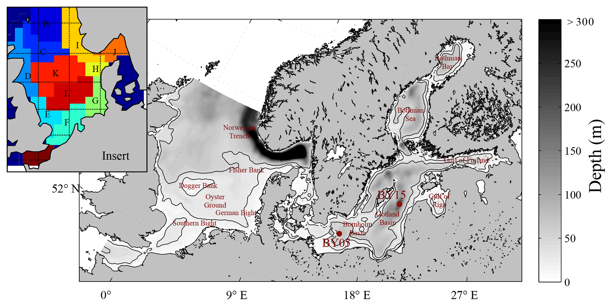
Figure 1 Model area and bathymetry. Black lines indicate depths of 30 and 60 m respectively. The insert represents the area subdivision in the ICES boxes for model comparison to ICES data (see Fig. 10).

We present the first application of a Eulerian end-to-end model for the shelf sea system of the North Sea and the Baltic Sea. The coupled North Sea–Baltic Sea system (Fig. 1) is located adjacent to the North Atlantic Ocean. Despite the close proximity of these seas, they are very different with respect to their physical and biogeochemical characteristics. The North Sea features pronounced co-oscillating tides combined with a major inflow from the North Atlantic. The Baltic Sea in contrast, only has a narrow opening to the North Sea which leads to an almost enclosed, brackish system with weak tidal forcing (Müller-Navarra and Lange, 2004). The restricted exchange capacity and fresh water excess of the Baltic Sea lead to an estuarine-type circulation with strong stratification and relatively low salinities in addition to a relatively long water residence time of about 30 years (Omstedt and Hansson, 2006; Rodhe et al., 2006). Due to its brackish waters, winter sea ice regularly develops in the Baltic Sea, which can, in severe winters, cover almost the entire surface (Seinä and Palosuo, 1996).

The two systems also differ substantially in terms of ecosystem dynamics. The North Sea is known as a highly productive area inhabited by more than 26 zooplankton taxa (Colebrook et al., 1984) and over 200 fish species (Daan et al., 1990), with the majority of the biomass distributed among demersal gadoids, flatfish, clupeids, and sand eel (Ammodytes marinus) (Daan et al., 1990). Consequently, the North Sea is economically highly relevant with nine nations fishing in the area and current landings of about 2 ×10⁶ t annually (ICES, 2018b). Compared with the North Sea, the species composition in the Baltic Sea is primarily limited by the low salinities and encompasses only a few key zooplankton (Möllmann et al., 2000) and fish (Fennel, 2010) species. Thus, compared to the North Sea, commercial fishing in the Baltic Sea is limited to a few stocks with total landings of over 0.6 ×10⁶ t annually (ICES, 2018a). In both regions, landings peaked in the 1970s and have substantially (ca. 50 %) declined since then. Thus, fishing has a substantial impact on the overall fish biomass in the region.

Studies on the food web dynamics of the North Sea and Baltic Sea have additionally highlighted the relevance of benthic fauna for fish consumption (Greenstreet et al., 1997; Tomczak et al., 2012). The term benthos generally refers to all organisms inhabiting the sea floor. A comprehensive review on the topic is given in Kröncke and Bergfeld (2003). The faunal components encompass over 5000 species which are generally divided by size into microfauna, meiofauna, and macrofauna. Additional differentiation can be made by considering the vertical habitat structure, with infauna inhabiting the inner part of the sediment and epifauna living above the sediments. While macrobenthos assemblages in the North Sea are structured based on the spatial distribution of sediment characteristics and depth, the Baltic sea community is additionally influenced by oxygen availability (Ekeroth et al., 2016) and salinity (Gogina et al., 2010). Besides their role as prey and predator in the marine food web, macrobenthos additionally influences nutrient effluxes from the sediments and can therefore modify the temporal and spatial patterns of nutrient concentrations (Ekeroth et al., 2016).

Here we present a functional type, E2E modelling approach, which relates food availability to potential fish growth and biomass distributions. In this paper we introduce the conceptual basis of the model, discuss its characteristics, and explore its performance with respect to the observed fish and MB distributions. Furthermore, we analyse model performance at the lower trophic levels in comparison to the NPZD modelling approach, and discuss the potential of our model for understanding and comparing basic regional ecosystem characteristics.

Figure 2 Schematic diagram of biological–geochemical interactions in ECOSMO E2E.

2 Methods

2.1 Model description

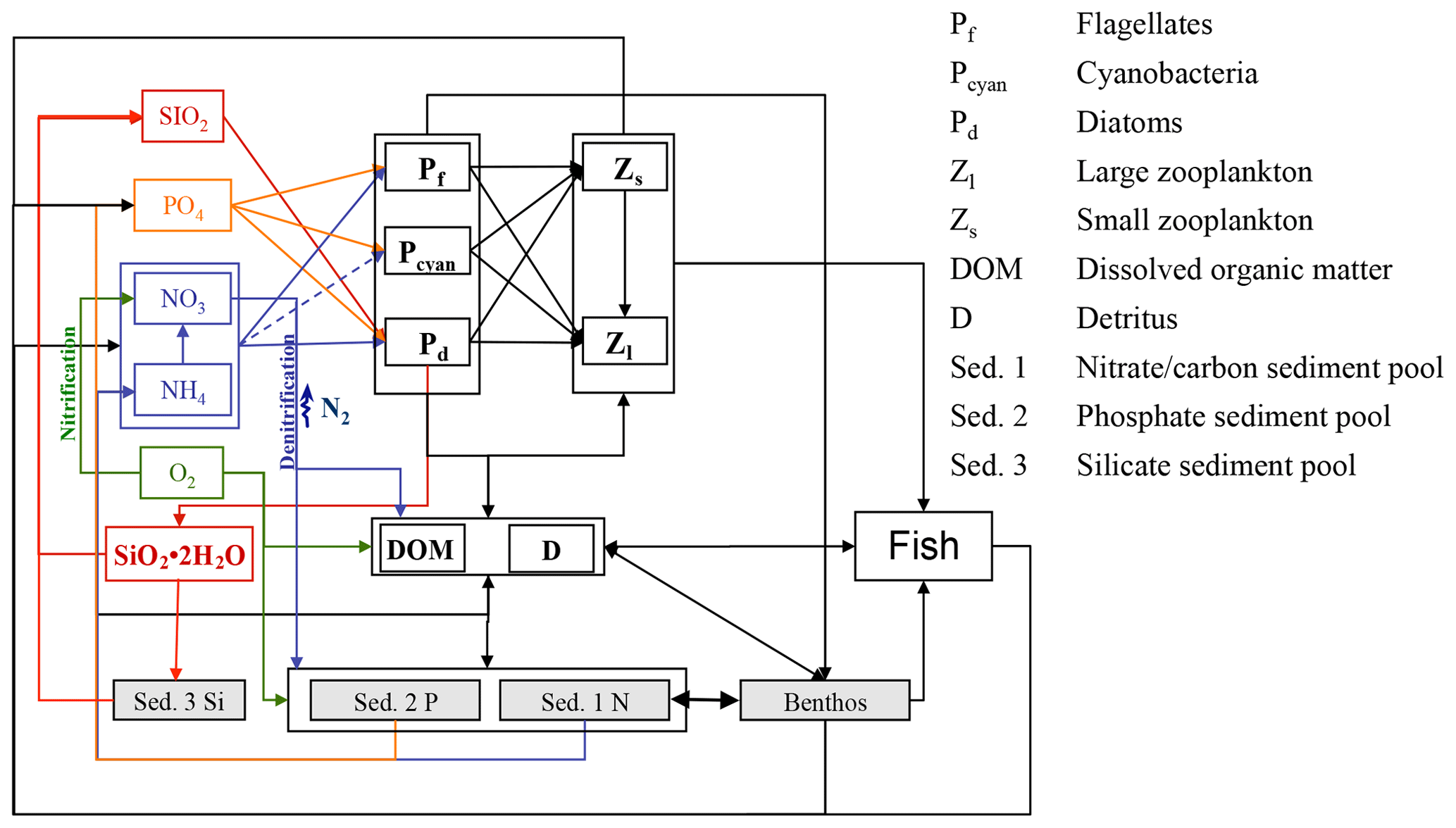
The E2E model builds on the coupled hydrodynamic–lower-trophic-level ecosystem model ECOSMO II (Barthel et al., 2012; Daewel and Schrum, 2013; Schrum et al., 2006; Schrum and Backhaus, 1999), which is further expanded for the present study. The latter model has been shown to accurately reproduce lower-trophic-level ecosystem dynamics in the coupled North Sea–Baltic Sea system. The model equations and a model validation on the basis of nutrients were presented in detail by Daewel and Schrum (2013), who showed that the model is able to reasonably simulate ecosystem productivity in the North Sea and the Baltic Sea on seasonal up to decadal timescales. The NPZD module was designed to simulate different macronutrient limitation processes in targeted ecosystems and comprises 16 state variables. Besides the three relevant nutrient cycles (nitrogen, phosphorus, and silica), three functional groups of primary producers (diatoms, flagellates, and cyanobacteria) and two zooplankton (herbivore and omnivore) groups were resolved. Additionally, oxygen, biogenic opal, detritus, and dissolved organic matter were considered. Sediment is implemented in the model as an integrated surface sediment layer, which accounts for the consideration of sedimentation as well as resuspension. Biogeochemical remineralisation is considered in surface sediments leading to inorganic nutrient fluxes into the overlying water column. To allow for nutrient-specific processes in the sediment, the organic silicate content of the sediment is estimated in a separate state variable. A third sediment compartment is considered for iron-bound phosphorus in the sediment (Neumann and Schernewski, 2008). To estimate total fish production and biomass in a consistent manner compared with lower-trophic-level production, we expanded the NPZD-type model via the implementation of a wider food web in the system (Fig. 2).

Although zooplankton in ECOSMO II could in principle also grow at the bottom, its parameterization as a passive tracer and the choice of parameterization for the functional groups makes it unsuitable for representing benthic production. Hence, the parameterisation of a specific functional group representing benthic (meio- and macro-) fauna remains necessary. The group was designed in a similar fashion to the zooplankton groups, but with the additional restriction that benthos only grows at the bottom and is not exposed to advection or diffusion. Benthic fauna has been observed to exhibit little tolerance to hypoxic and anoxic conditions (Kröncke and Bergfeld, 2003); therefore macrobenthos growth was only estimated for positive oxygen concentrations in the model framework. In contrast to the benthic compartment in ERSEM (Butenschön et al., 2016), where the benthic predators are distributed into three different functional types, in this study we neglect different functional traits of infauna and epifauna and only consider one functional group, which we, for convenience, will refer to as macrobenthos (MB).

Each state variable C in ECOSMO II is estimated following prognostic equations in the form of

$$\begin{array}{}\text{(1)}& C_t+\left(\mathit{V}\cdot \mathrm{\nabla }\right)C+\left(w_{\text{d}}\right)C_z=(A_v{C}_z{)}_z+R_{\text{c}}\end{array}$$

with $C_t=\frac{\partial C}{\partial t}$, $C_z=\frac{\partial C}{\partial z}$, where t is time and z is the vertical coordinate. The equation includes advective transport $(\mathit{V}\cdot \mathrm{\nabla })C(\mathit{V}=(u,v,w)$ the current velocity vector), vertical turbulent sub-scale diffusion (A_vC_z)_z (A_v is the turbulent sub-scale diffusion coefficient), sinking rates (w_d)C_z (the w_d sinking rate is non-zero for detritus, opal, and cyanobacteria), and chemical and biological reactions (R_c). As MB production occurs locally at the bottom and the group is not exposed to mechanical displacement, Eq. (1) is simplified for MB:

$$\begin{array}{}\text{(2)}& {\displaystyle \frac{\text{d}{C}_{\text{MB}}}{\text{d}t}}={\left[R_{\text{MB}}\right]}_{z=z_{\text{bottom}}}\end{array}$$

Concurrently chemical and biological interactions are employed in the biological reaction term R_C, which is different for each variable (C) based on the relevant biochemical processes. For MB it is divided into production, which is a function of consumption (R_{MB_Cons}) and assimilation efficiency (γ_MB), and a MB loss term as follows:

$$\begin{array}{}\text{(3)}& R_{\text{MB}}={\mathit{\gamma }}_{\text{MB}}{R}_{\text{MB\_Cons}}-R_{\text{MB\_Loss}}\end{array}$$

The production of zooplankton in the model depends on the available food resources, which include phytoplankton, detritus, and (for the omnivorous zooplankton group) also herbivorous zooplankton. For the macrobenthos functional group, we assume a much wider range of potential prey items. The benthic community can be divided into the following groups: benthic suspension-/filter-feeders that mainly feed on phytoplankton, detritus, and bacteria; benthic deposit-feeders that ingest bottom sediments; and larger individuals that exert predation pressure (among others) on the available zooplankton (Kröncke and Bergfeld, 2003). Thus, the prey spectrum of the simulated MB functional group also includes, besides phyto- and zooplankton, detritus, and organic sediments. As we assume that benthic suspension-/filter-feeders would also indirectly ingest dissolved organic matter, we chose to add the latter to the MB diet.

Consumption of the MB group is estimated as the sum of the consumption rates of the single prey items: herbivorous zooplankton (Z₁), omnivorous zooplankton (Z₂), flagellates (P₁), diatoms (P₂), detritus (D), dissolved organic matter (DOM), and organic sediment (Sed. 1).

$$\begin{array}{ll}\text{(4)}& {\displaystyle }{R}_{\text{MB\_Cons}}& {\displaystyle }=C_{\text{MB}}\left(\sum _{j=\mathrm{1}}^{\mathrm{2}}{G}_{\text{MB}}\left(C_{Z_j}\right)+\sum _{l=\mathrm{1}}^{\mathrm{2}}{G}_{\text{MB}}\left(C_{P_{\text{l}}}\right)\right.{\displaystyle }& {\displaystyle }+G_{\text{MB}}\left(C_{\text{D}}\right)+G_{\text{MB}}\left(C_{\text{DOM}}\right)+G_{\text{MB}}\left(C_{\text{Sed. 1}}\right))\end{array}$$

Grazing rates (G_MB) on prey type X (Xϵ [Z₁; Z₂; P₁; P₂; D; DOM; Sed. 1]) are estimated using the Michaelis–Menten equation (Michaelis and Menten, 1913; Monod, 1942):

$$\begin{array}{}\text{(5)}& G_{\text{MB}}\left(C_X\right)={\mathit{\sigma }}_{\text{MB},X}{\displaystyle \frac{a_{\text{MB},X}{C}_X}{r_{\text{MB}}+F_{\text{MB}}}},\end{array}$$

where $F_{\text{MB}}=\sum _X{a}_{\text{MB},X}{C}_X$.

Table 1 Parameters used for the MB functional group reaction terms.

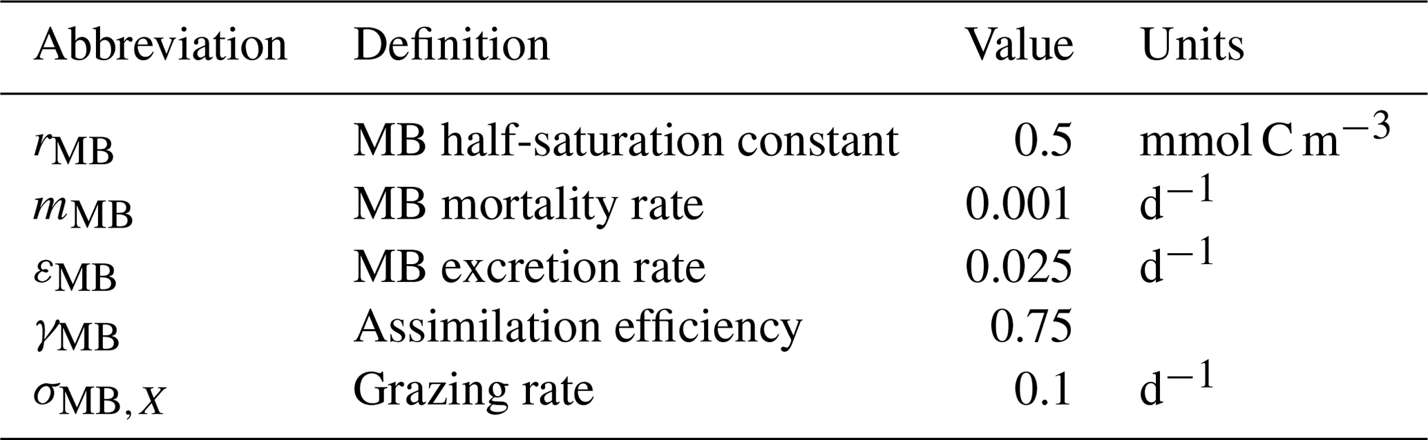
Table 2 Feeding preferences for macrobenthos (MB) and fish (Fi) a_Y,X.

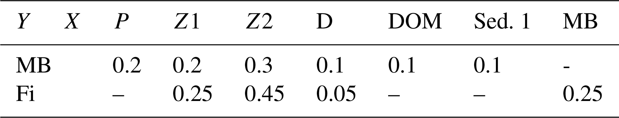
The half-saturation constant (r_MB) and values for grazing rates (σ_MB,X) are given in Table 1, and feeding preferences (a_MB,X) are given in Table 2.

The MB loss term consists of excretion (ε_MBC_MB), natural mortality (m_MBC_MB), and predation mortality from the fish functional group (C_FiG_Fi(C_MB)). Values for excretion (ε_MB) and mortality rate (m_MB) are given in Table 1.

$$\begin{array}{}\text{(6)}& R_{\text{MB\_Loss}}=C_{\text{Fi}}{G}_{\text{Fi}}\left(C_{\text{MB}}\right)+m_{\text{MB}}{C}_{\text{MB}}+{\mathit{\epsilon }}_{\text{MB}}{C}_{\text{MB}}\end{array}$$

We assume that “fish” is a prognostic variable, which is, in contrast to the other prognostic state variables in the ecosystem model, not exposed to passive transport processes and does not actively move horizontally. This can be translated into the assumption that characteristic fish migration is restricted to a spatial scale below the model grid size – of the order of 10 km. Larger-scale migration behaviour is neglected here. As we know that neglecting larger horizontal migrations places major constraints on the model's ability to estimate the spatial distribution of the overall fish biomass, we believe that the assumption is still valid for calculating the overall fish production potential and its spatial distribution in the system. Thus, in the following we will refer to “fish” as a functional group that comprises the fish biomass that emerges based on the lower trophic production at each horizontal grid cell. For clarification it needs to be noted that, even when referred to as “fish production potential”, the fish biomass is a state variable in the model that interacts dynamically with the lower-trophic-level components and that will be used in the following to confirm the models ability to simulate spatial and temporal patterns of carbon transfer to higher trophic levels. By constraining the horizontal migration capabilities of the fish group to one grid cell we will likely underestimate the local fish production potential by confining it to the locally available fish biomass.

The potential “fish” still needs to be considered more mobile than the other ecosystem components in the model; therefore, the vertical distribution of the fish group is assumed to result from fish active movement and varies based on food availability. This leads to the following principles being applied for the fish functional group:

1. We neglect horizontal fish migration at spatial scales larger than one grid cell.

2. The fish group is mobile and, within the given time step (20 min), able to search the water column for food beyond the vertical extent of a single grid cell. Therefore, we assume that the fish group is able to utilise the food resources available at all depth levels within the water column. Consequently, the fish group is not (as other variables are) calculated within one sole grid cell, but depends on the vertically integrated food resources.

3. The vertical distribution of the fish group and fish production depends on the food availability in each grid cell. This means that during each time step the integrated fish biomass in the water column is vertically redistributed based on the vertical prey distribution after consumption has been estimated.

Following these three principles implies that Eq. 1 is simplified to $\frac{\partial C_{\text{Fi}}}{\partial t}+w_{\text{m}}\left(z\right)\frac{\partial C_{\text{Fi}}}{\partial z}=R_{\text{Fi}}$, where w_m(z) is the vertical migration speed, which is given implicitly by the vertical distribution of the fish biomass and is dependent on the vertical prey distribution. In each grid cell the biological interaction term (R_Fi) is estimated and contains fish consumption ($R_{{\text{Fi}}_{\text{Cons}}}$), assimilation efficiency γ_Fi, and a loss term ($R_{{\text{Fi}}_{\text{Loss}}}$):

$$\begin{array}{}\text{(7)}& R_{\text{Fi}}={\mathit{\gamma }}_{\text{Fi}}{R}_{{\text{Fi}}_{\text{Cons}}}-R_{{\text{Fi}}_{\text{Loss}}}\end{array}$$

Following principle 2 and 3, R_Fi is estimated via a two-step process. First, total fish consumption at the horizontal location (m, n) is estimated based on the vertically integrated values for fish and prey biomass:

$$\begin{array}{ll}\text{(8)}& {\displaystyle }{R}_{{\text{Fi}}_{\text{prod}}}(m,n)& {\displaystyle }=\sum _{k=\mathrm{1}}^{k_{\text{max}}}\left(R_{{\text{Fi}}_{\text{Cons}}}\right(m,n,k)\times \mathrm{\Delta }{z}_k){\displaystyle }& {\displaystyle }=\sum _X(G_{\text{Fi}}\left(P_X\right)\times P_{\text{Fi}}),\end{array}$$

where P_X (X is one of four prey types – herbivorous zooplankton Z₁, omnivorous zooplankton Z₂, detritus D, and macrobenthos MB – available for fish in the model) is defined as the integrated biomass of the prey type X ($P_X=\sum _{k=\mathrm{1}}^{k_{\text{max}}}(C_{X_k}\times \mathrm{\Delta }{z}_k)$) over all vertical levels ($k=\mathrm{1}:k_{\text{max}}$) at the respective horizontal location (m, n). P_Fi is the corresponding vertically integrated biomass of fish. Grazing rates G_Fi are estimated using the Michaelis–Menten equation $G_{\text{Fi}}\left(P_X\right)={\mathit{\sigma }}_{\text{Fi},X}\frac{a_{\text{Fi},X}{P}_{\text{Fi}}}{r+F}$ with $F=\sum _X{a}_{\text{Fi},X}{P}_X$, and a_Fi,X is the feeding preference of fish on prey type X (values in Table 2), in a similar manner as for the zooplankton and MB groups.

In a second step, fish consumption in each grid box (m, n, k) is estimated by weighting the prey-specific components of the consumption in each vertical layer based on the vertical distribution of the prey biomass with $C_X(m,n,k)/P_X(m,n)$ such that

$$\begin{array}{ll}\text{(9)}& {\displaystyle }& {\displaystyle }{R}_{{\text{Fi}}_{\text{Cons}}}(m,n,k)={\displaystyle }& {\displaystyle }{P}_{\text{Fi}}\left(\sum _{j=\mathrm{1}}^{\mathrm{2}}{G}_{\text{Fi}}\left(P_{Z_j}\right)\times {\displaystyle \frac{C_{Z_j}}{P_{Z_j}}}+G_{\text{Fi}}\left(P_{\text{D}}\right)\times {\displaystyle \frac{C_{\text{D}}}{P_{\text{D}}}}\right.\\ {\displaystyle }& {\displaystyle }+{\left[G_{\text{Fi}}\left(P_{\text{MB}}\right)\right]}_{k=\text{bottom}})\end{array}$$

Note that, as fish do not tolerate anoxic conditions, only grid cells featuring positive oxygen concentrations were considered for the estimate of fish consumption.

The loss term for fish includes mortality and excretion.

$$\begin{array}{}\text{(10)}& R_{{\text{Fi}}_{\text{Loss}}}=m_{\text{Fi}}{C}_{\text{Fi}}+{\mathit{\epsilon }}_{\text{Fi}}{C}_{\text{Fi}}\end{array}$$

Mortality is considered as a linear mortality rate including biomass losses due to natural mortality and predation. Fisheries mortality was not considered for the standard simulation, but was explicitly addressed in additional scenario experiments as described in Sect. 2.4. Excretion is considered to be related to fish metabolism and consequently to respiration (see the equation for oxygen in Table 4) and hence has been parameterised as dependent on temperature (Clarke and Johnston, 1999; Gillooly et al., 2001). Reaction kinetics vary with temperature according to the Boltzmann factor k, and we formulated the fish excretion as follows:

$$\begin{array}{}\text{(11)}& {\displaystyle }{\mathit{\epsilon }}_{\text{Fi}}={\mathit{\mu }}_{\text{Fi}}{e}^{\left(\frac{{\mathit{\theta }}_{\text{Fi}}}{k}\times TK\right)};TK={\displaystyle \frac{T-T_{\mathrm{0}}}{T\times T_{\mathrm{0}}}}\end{array}$$

, where T is given in K and T₀=273.15 K. All rates are given in Table 3.

Table 3 Parameters used for the fish functional group.

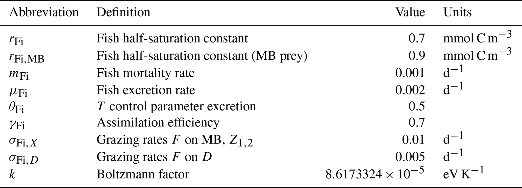
Table 4 Changes in the biogeochemical reaction terms (R) of ECOSMO due to the macrobenthos (MB) and fish functional groups.

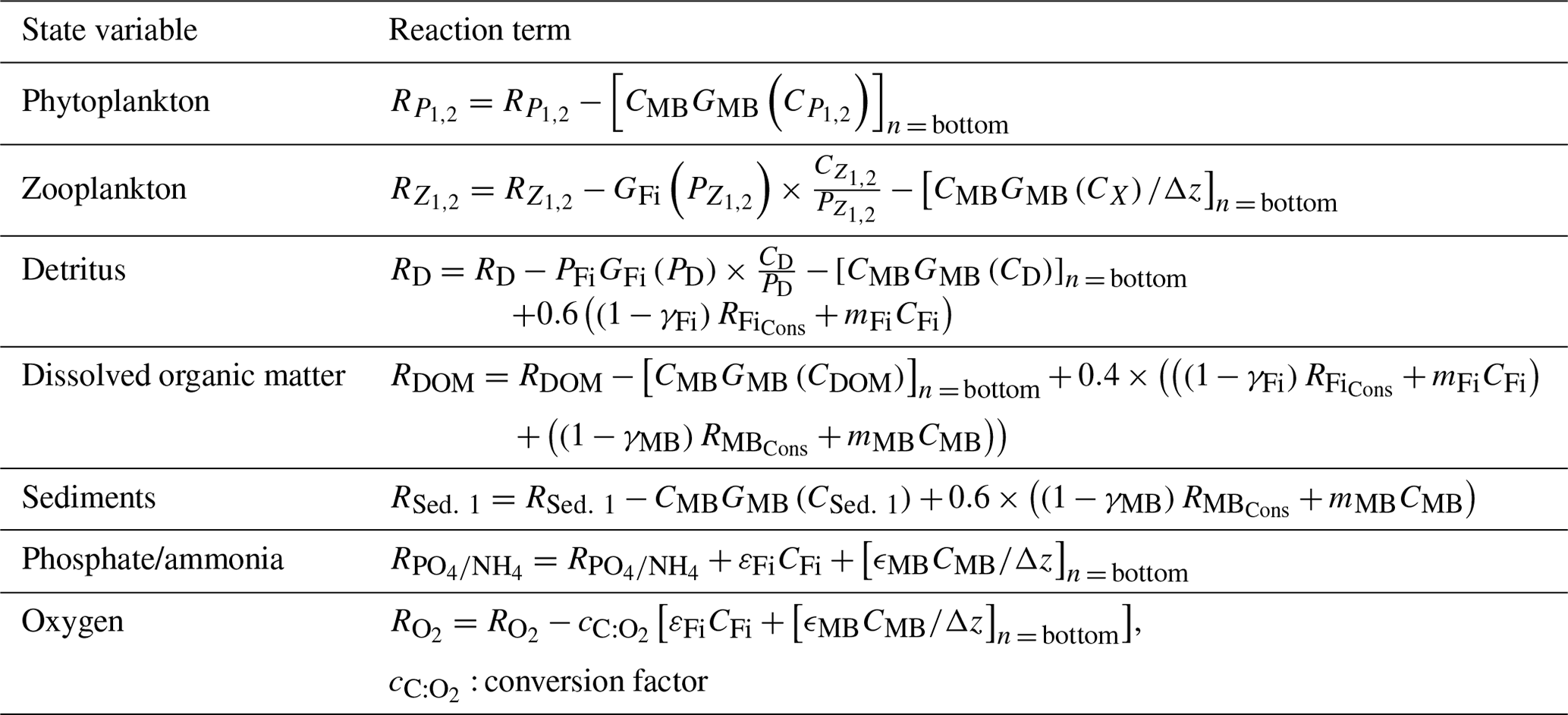
Fish and macrobenthos predation, excretion, and mortality are considered in addition to the pelagic lower-trophic-level biological reaction terms (see Daewel and Schrum, 2013) for nutrients, phytoplankton, zooplankton, detritus, dissolved organic matter, or sediment (Table 4). While fecal matter is accounted for through the use of assimilation efficiency, the excretion term from both fish and MB directly contributes to the nutrient reaction terms (see equation for phosphate and ammonia in Table 4). The new zooplankton mortality term consists of fish predation and additional background mortality, which is 80 % of the background mortality term used in ECOSMO II. In situ and laboratory studies indicate that predation mortality accounts for 67 %–75 % of the total mortality (Hirst and Kiørboe, 2002). Other sources of mortality are parasitism, disease, and starvation. However, including fish and macrobenthos as predators in the model does not account for the overall predation exerted on zooplankton. By analysing the pelagic food web of the North Sea, Heath (2005) identified the fish consumption of omnivorous zooplankton to be 6.7 g C m⁻² year⁻¹ on average. This value was recalculated in Heath (2007), after the role of fish pre-recruits feeding on zooplankton was more specifically considered, and was reported to amount to ∼ 7.6 g C m⁻² year⁻¹, whereas the average consumption by carnivorous zooplankton (euphausids and macroplankton) was considerably higher at 11 g C m⁻² year⁻¹. As the zooplankton groups in the model are not stage resolving, intra-guild predation is not explicitly prescribed as a mortality term, but is implicitly included in the background mortality. Although our model results also suggest that a substantial amount of zooplankton is consumed by macrobenthos in the shallow regions of the North Sea, assuming that about 20 %–30 % of zooplankton mortality stems from the combined fish and benthos group seems to be a good first guess. The fact that the reduction of the background mortality rate to 80 % of its initial value does not necessary imply that the background mortality is 80 % of the total mortality should be taken into consideration. By including a spatially and temporally variable mortality term in the model, this term can locally play a much larger (or smaller) role for the overall mortality. To evaluate the model sensitivity to the choice of this parameter, we performed scenario experiments described in Sect. 2.4. The degradation products from MB, fish mortality, and food consumption contribute to particulate organic matter (POM) and dissolved organic matter (DOM), and it is distributed between the two partitions POM and DOM with a ratio 60 % ∕ 40 % (for an explanation see Daewel and Schrum, 2013b). As MB species live at the sea floor we assume that the POM generated directly contributes to the sediment pool (Sed. 1), which might contribute to the suspended particulate matter (D) via resuspension depending on bottom stress. The fish contribution to the POM is added to the detritus pool.

2.2 Experimental set-up

To evaluate the model performance after including two new functional groups, we chose to analyse model results from a 10-year-long simulation period (1980–1989) based on two key requirements. First, as the characteristic timescale of the Baltic Sea is in the range of 3 decades, and the model results also indicate an adaptation period of about 20–30 years for fish and MB in the Baltic Sea (not shown), the simulation was started in 1948 to allow for a sufficiently long spin-up period with a realistic forcing. Second, we wanted to analyse a relatively undisturbed period with respect to hydrodynamic and biogeochemical conditions. Therefore, we chose a period prior to the observed regime shift at the end of the 1980s and the major Baltic inflow in 1993.

The model set-up is similar to that described by Daewel and Schrum (2013) for long-term simulations using a hydrodynamic core model based on HAMSOM (Hamburg Shelf Ocean Model), as described in Schrum and Backhaus (1999), with additional modification of the advection scheme (Barthel et al., 2012). The model is formulated on a staggered Arakawa-C grid with a horizontal resolution of 6^′ × 10^′ (∼ 10 km) and a 20 min time step. The vertical dimension was resolved with 20 vertical levels; within these levels, the upper 40 m has a layer thickness of 5 m, and the resolution becomes coarser below this point. The model requires boundary conditions at the atmosphere–ocean boundary (NCEP/NCAR reanalysis; Kalnay et al., 1996) and at the open boundaries to the North Atlantic. Transport of freshwater and nutrient loads from land is considered. Details on the boundary and forcing data utilised are given by Daewel and Schrum (2013), who also provided a detailed description of analysis methods and validation datasets.

2.3 Datasets and statistical methods for model analysis

As described in Daewel and Schrum (2013), we used observational data on surface (depth < 10 m) nutrients (nitrate and phosphate) in the North Sea, which are made available by the ICES (International Council for the Exploration of the Seas, http://www.ices.dk/Pages/default.aspx, last access: 30 November 2011), for nutrient validation. Observations and modelled surface nutrients were averaged over the upper 10 m of the water column and co-located in space and in time, and corresponding statistics were calculated for the sub-areas specified in Fig. 1. The seasonal cycle was not removed prior to the analysis. The reason for this was the sparse data situation, which did not allow for the estimation of a reliable seasonal cycle at each location, in addition to the seasonal cycle changes from year to year. Thus, removing an average seasonal cycle from the data would add a bias to the data and subsequently increase the level of uncertainty. In the Baltic Sea, we used vertical nutrient profiles (NO₃, PO₄, and O₂) at two distinct locations in the Baltic proper: BY05 (lat/long: (∼ 55.1^∘ N/15.59^∘ E) and BY15 (lat/long: ∼ 57.2^∘ N/20.03^∘ E) (see Fig. 1); these location were from the Baltic Sea monitoring network (see e.g. http://www.helcom.fi/, last access: 29 April 2019) and have been continuously sampled since 1970. The data are available for download at http://www.ices.dk (last access: November 2016). To account for inconsistencies in sampling frequencies, we co-located model data and observations prior to estimating average vertical profiles and standard deviations. For this purpose, the model values were linearly interpolated onto a 1 m vertical grid to allow for the best local comparison to the observations, whereas the observations where considered at the actual sampling depth. The statistical measures chosen for model analysis were the Pearson correlation coefficient, the standard deviation and the root mean square deviation presented in a Taylor diagram (Taylor, 2001), and the empirical orthogonal functions (EOFs) as described in von Storch and Zwiers (1999). The EOF analysis is a statistical method used to understand the major modes of variability in multidimensional data fields. A detailed description on how this method has been applied is given in Daewel et al. (2015): “The annual values of the spatially explicit PLS field form an N×M matrix χ (N: number of years; M: number of wet grid points). The empirical modes are given by the K eigenvectors of the covariance matrix with non-zero eigenvalues. Those modes are temporally constant and have the spatially variable pattern p_k ($m=\mathrm{1},\mathrm{\dots },M$) where $k=\mathrm{1},\mathrm{\dots },K$. The time evolution A_k ($t=\mathrm{1},\mathrm{\dots },N$) of each mode can then be obtained by projecting p_k(m) onto the original data field χ such that: $\mathit{\chi }(t,m)=\sum _{k=\mathrm{1}}^K{p}_k\left(m\right)A_k\left(t\right)$. In the following sections we will refer to A_k(t) as the principal components (PCs) and to p_k(m) as the EOF. The percentage of the variance of the field χ explained by mode k is determined by the respective eigenvalues and is referred to as the global explained variance η_g(k). Before using the method to analyse the spatio-temporal dynamics of the field, the data were demeaned (to account for the variability only) and normalised (to allow an analysis of the variability independent of its amplitude). The identified modes are not necessarily equally significant in all grid points of the data field. Thus, the local explained variance η_local,k(m) could provide additional information about the regional relevance of an EOF mode and the corresponding PC in percent:

$$\begin{array}{}\text{(12)}& {\mathit{\eta }}_{\text{local}}^k\left(m\right)=\left[\mathrm{1}-{\displaystyle \frac{\text{Var}\left(\mathit{\chi }(m,t)-p^k\left(m\right)A^k\left(t\right)\right)}{\text{Var}\left(\mathit{\chi }(m,t)\right)}}\right]\times \mathrm{100},\end{array}$$

where $\text{Var}\left(X\right)=\sum _{t=\mathrm{1}}^N{\left(\stackrel{\mathrm{‾}}{X}-X\left(t\right)\right)}^{\mathrm{2}}$ denotes the variance of the field X(t).” In Daewel et al. (2015), the method was applied to the potential larval survival (PLS) of Atlantic cod (Gadus morhua), while in this study it is used on estimated MB and fish biomass.

Information on the North Sea fish community were collected during the North Sea international Bottom Trawl Survey (NS-IBTS) (ICES, 2012) and are freely available at the International Council for the Exploration of the Sea (http://www.ices.dk/Pages/default.aspx, last access: May 2012). The NS-IBTS dataset contains spatially resolved, species-specific information on fish length (for some target species also age) and catch per unit effort (CPUE: in numbers captured per hour). Given that our model estimated state variables on the base of carbon biomass, we converted fish length and abundance data to fish biomass (in grams captured per hour) based on published length–weight relationships (LWRs) for each species sampled in the NS-IBTS between 1980 and 1989 (inclusive of these years).

LWRs were derived from Coull et al. (1989), Froese et al. (2014), and FishBase (Froese and Pauly, 2000) for teleost species; McCully et al. (2012) and Templeman (1987) for rays and skates; Klaoudatos et al. (2013) for crabs; and Pierce et al. (1994) and Guerra and Rocha (1994) for squids. Total body weight (W) is a function of total length (L) following the relationship W=aL^b, where b is a parameter indicating isometric growth in body proportions if b∼3, and a is a parameter describing body shape and condition if b∼3.

Calculations were made at the species level, where species names were available, with the a and b parameter estimates taken from published sources in the following order:

1. Studies specific to the North Sea (i.e. Coull et al., 1989; Froese and Pauly, 2000).

2. If information was not available in the abovementioned research, studies specific to the British Isles were utilised (i.e. Coull et al., 1989; Froese and Pauly, 2000; McCully et al., 2012).

3. If information was not available in the abovementioned research, studies specific to the North Atlantic (i.e. Coull et al., 1989; Froese and Pauly, 2000; McCully et al., 2012; Templeman, 1987).

4. If information was not available in the abovementioned research, posterior mean estimates of a and b from a Bayesian hierarchical analysis for the species across all credible LWR studies were utilised, regardless of location (see Froese et al., 2014; Froese and Pauly, 2000).

For some species, e.g. herring, sprat, and mackerel, Coull et al. (1989) provided mean parameter estimates for each month, or at least some months throughout the year, in addition to annual estimates. In these cases, we used annual estimates only. If information was only available for genus, family, or order, the a and b parameter estimates for all species within that genus, family, or order captured during the surveys were averaged to give a genus-, family-, or order-specific value. If no information was available at any species level within a genus, family, or order, the geometric mean of that genus, family, or order was computed from the data file accompanying Froese et al. (2014). The data were sorted onto the horizontal model grid based on their sampling location. For the data–model comparison we only considered data from the first quarter of the year, as this was the only systematically surveyed quarter in the considered time period (1980–1989) in the survey.

2.4 Scenario definition

Two sets of scenarios were performed to evaluate the simulated food web response to specific changes in the food web parameterisations. We study the structuring effects of the new model closure term (higher trophic levels/fisheries) and the effects of changes in background zooplankton mortality. The first set of scenario experiments addresses the carbon loss through apex predators and fisheries by adding another source of mortality in addition to the natural fish mortality term. Following the fisheries overview of the North Sea and Baltic Sea regions as published by ICES (2018a, b), biomass losses due to fisheries are in the range of 20 %–50 % of the total fish biomass per year in both regions. Therefore, for convenience we decided to calculate the fisheries mortality rate by scaling the natural mortality rate (= 0.001 d⁻¹ = 0.365 years⁻¹) by 0.5, 1, and 2. As such, three different scenarios were calculated with an average (0.1825 years⁻¹), high (0.365 years⁻¹), and extreme (0.5475 years⁻¹) loss rate. Note that the latter two loss rates were chosen to provoke extreme responses in the fish biomass, and do not represent realistic catch rates in the areas.

The second set of experimental scenarios was designed to understand the ecosystem response to changes in the zooplankton natural mortality. This term previously formed the sole closure term of the system, and the rate has been reduced by 20 % to account for the additional mortality induced to the system by MB and fish predation. Here, we chose four scenarios for the experiment: (1) the control run, which considered the unchanged zooplankton mortality rate from ECOSMO II; (2) control −20 %, which is the reference set-up for ECOSMO E2E; (3) control −40 %; and (4) control +20 %; scenarios (3) and (4) were used for comparison.

3 Results and discussion

In the following, we discuss the basic characteristics of the model and assess its performance based on 10-year averages of the model variables. Specifically, we (i) present and discuss the spatial dynamics of the newly introduced functional groups, (ii) discuss the seasonality of the ecosystem components and introduce the MB and fish diet composition emerging from the model, (iii) present the comparison of the simulated fish biomass distribution to observed data and repeat the nutrient validation analysis as previously presented for ECOSMO II in Daewel and Schrum (2013), and (iv)  discuss the model sensitivity with respect to ecosystem model closure.

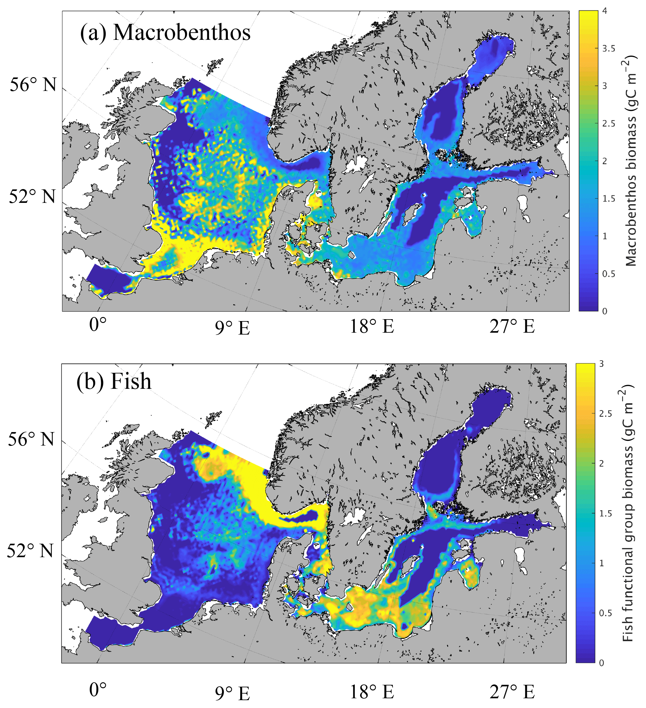
Figure 3 Simulated spatial pattern of annual mean biomass of macrobenthos (a) and fish (b) (g C m⁻²).

3.1 Description of modelled spatial pattern

The mean spatial patterns of calculated MB and fish vertically integrated biomass for the period from 1980 to 1989 are presented in Fig. 3. On average, estimated MB biomass (Fig. 3a) in the North Sea is 1.98 g C m⁻² for the time period considered. As we will see later, this value is highly sensitive to the parameterisation of zooplankton mortality and fisheries effort (cf. Sect. 3.4 and Fig. 12). Heip et al. (1992) proposed an average of 7 g ash-free dry weight (AFDW) m⁻² based on a synoptic sampling of North Sea benthos in April–May 1986. This equates to approximately 3.5 g C m⁻² when assuming a carbon fraction of the ash-free dry weight of 0.5 (Ingrid Krönke, Senckenberg am Meer, Wilhelmshaven, Germany, personal communication, 2016), which is somewhat higher than our model estimates, but also includes benthic carnivore biomass (Greenstreet, 1997). Greenstreet (1997) estimated the biomass of the benthic filter-feeder and deposit-feeder guild to be ∼ 3 g C m⁻² when the same carbon fraction of 0.5 was applied. Note that the comparison can only be an approximation due to the high variability in carbon content among species (e.g. Timmermann et al., 2012). Observational estimates of North Sea MB biomass indicate a decrease in biomass with increasing latitude according to Heip et al. (1992), and similar results were obtained from a subsequent sampling project in 2000 (Rees et al., 2007). Particularly high values of MB biomass were found in the shallow areas of the southern North Sea, including the coastal areas and Dogger Bank (Heip et al., 1992, their Fig. 1), and in the river mouth areas along the English coast. This is in clear agreement with what was estimated by our model.

In the Baltic Sea, the MB biomass was modelled to be 1.01 g C m⁻² on average. This is in the range of what was published by Timmermann et al. (2012) based on HELCOM data, where spatially resolved values between 5 and 100 g WWt m⁻² (approx. 0.25–5 g C m⁻²) were reported; it is also within the range of values published by Tomczak et al. (2012), who estimated macrobenthos biomass of about 30 t km⁻² (which equals 1.5 g C m⁻² using an Ecopath with Ecosim Baltic Proper food web model). Furthermore, the spatial distribution of MB modelled using our simplified model is consistent with the spatial distribution of major MB species in the Baltic Sea as presented by Gogina and Zettler (2010) based on species-specific model estimates and observations. This applies specifically to the high abundances in the southern Baltic Sea, the near coastal areas, and the Gulf of Riga.

Our model estimates the highest MB biomass in both the North Sea and the Baltic Sea in shallower areas, especially near the coast and in bank regions, such as Dogger Bank, Fisher Banks, and Oyster Ground, with a maximum of around 5 g C m⁻² found in the southern North Sea. MB production in the model is constrained by the availability of oxygen; therefore, large areas of the central Baltic Sea are not inhabited by macrobenthos. In the North Sea, minimum MB biomass is estimated slightly offshore of the British coast and in the deeper parts of the Norwegian Trench region. These minima in the North Sea were not caused by anoxic conditions, but by a lack of prey in the respective areas. In contrast, the transition zone between the North Sea and the Baltic Sea, including the Skagerrak, Kattegat, the Danish straits, and the Fehmarn Belt, generally exhibits high MB biomass values.

Simulated spatial variability in vertically integrated fish biomass shows a structured pattern in both the North Sea and the Baltic Sea. In the Baltic Sea, maxima of fish biomass are simulated in the coastal areas, the Gulf of Riga, in the southern Baltic Sea (including Arkona Basin, Bornholm Basin, and Bay of Gdansk), and in the Åland Sea at the entrance to the Bothnian Sea. The deeper parts of the Eastern Gotland Basin, the Gulf of Finland, and the Gulf of Bothnia, in contrast, feature very low fish biomass due to low prey biomass and oxygen depletion near the bottom. The modelled spatial distribution compares well with findings from the nutrient-to-fish model from Radtke et al. (2013). They integrated the model over a 4-year period from 1980 to 1983. In their model approach, fish follows specific rules for horizontal migration (food availability and spawning). However, their simulated spatial distribution of the combined biomass for the three different simulated fish species is very similar to our estimates. Differences between the simulated fish distributions specifically occur in time periods when predefined spawning areas determine the distribution. Other spatial differences were simulated for the Gulf of Finland, where the model by Radtke et al. (2013) estimated relatively high fish biomass in contrast to our model, and around Gotland, where our model produces fish biomass maxima potentially fostered by the additional availability of macrobenthos as prey, which remains unconsidered by Radtke et al. (2013). Interestingly, the distribution of fish biomass maxima (estimated by our model) resembles the pattern of cod nursery areas described in the Baltic Sea by Bagge et al. (1994).

The structure of modelled North Sea fish biomass is very distinct with maxima in frontal areas such as the tidal mixing front in the southern North Sea and around Dogger Bank and the frontal zone off the German, Danish, and British coast, and in the Norwegian Trench. Maxima are also modelled in the Fisher Banks and Oyster Ground as well as the Fladen Ground regions. Minima, in contrast, were estimated in the deeper parts of the western North Sea off the British coast, the German Bight, and in the English Channel. They partly resemble the minima estimated for MB, which indicates that fish biomass minima are caused by food shortages in areas with low MB biomass. In particular, off the British Coast, studies from Callaway et al. (2002) and Jennings et al. (1999) indicate high fishing effort, indicating that the model likely underestimates the fish biomass in that region. Potential reasons for this are the model underestimating zooplankton production in that area (Daewel et al., 2015), and the missing impact of the open boundary, where neither zooplankton nor fish were prescribed to enter the model domain.

When integrating fish biomass over the North Sea and the Baltic Sea regions, it amounts to ca. 0.462 and 0.312 ×10⁶ t C respectively. Assuming that the carbon content of fish is 45 % (Huang et al., 2012; Sterner and George, 2000) and that the AFDW (ash-free dry weight) to wet weight fish ratio ranges from 0.1 to 0.2, this corresponds to a simulated total fish biomass in the range of 5.13–10.27 ×10⁶ t for the North Sea and 3.47–6.93 ×10⁶ t for the Baltic Sea. As the AFDW to wet weight ratio is highly variable, even within species, depending on factors such as temperature, season, and the diet of the fish (Elliott and Hemingway, 2002), it is difficult to determine an exact value for the simulated entire fish assemblage biomass. The modelled estimates of fish biomass are well within the range of what has been estimated for total fish biomass based on observations for the Baltic Sea (Thurow, 1997). Using yield data and age composition data in catches, Thurow (1997) estimated total fish biomass in the Baltic Sea for the time period from 1900 to 1985. His results indicate relatively low fish biomass (< 2 ×10⁶ t) for the first half of the century, but a drastic increase thereafter. For the time period considered here (i.e. 1980–1989) he proposed the fish biomass to be around 7 ×10⁶ t. Following ICES (2018b, a), fisheries during the 1980s were in the range of 0.7–1 ×10⁶ t in the Baltic Sea and 2–3 ×10⁶ t in North Sea. Despite the fact that the model underestimates fish production due to the assumption that there is no horizontal migration and that no fish migrate over the lateral boundaries, the model's estimates of fish biomass in the North Sea would support the landing data from fisheries during that time period.

Estimates for North Sea total biomass for the 1983-1985 period based on the ICES International Young Fish Survey (IYFS) and the English Groundfish Survey (EGFS) were published by Sparholt (1990). For the first quarter, Sparholt (1990) estimated an average fish biomass of about 8.6 ×10⁶ t, whereas for the third quarter the average biomass was estimated to be 13.1 ×10⁶ t. The discrepancy between first and third quarter was explained by the migration of the western stock of Atlantic mackerel (Scomber scombrus) and horse mackerel (Trachurus trachurus) into the North Sea, which is not considered by our model. Furthermore, our results are in agreement with output from an Ecopath with Ecosim food web model of the North Sea proposed by Mackinson and Daskalov (2007), which estimated that the North Sea total fish biomass was ∼ 11 ×10⁶ t in 1991. Indeed, our modelled estimate is well within the range of previously published observations and model results. We suggest that any discrepancies are most likely due to our model neglecting fish migration at large scales. When discussing the spatial variation of estimated fish biomass we need to consider that the model is constrained by the assumption that fish do not move horizontally. Thus, we estimate the production potential for fish in each horizontal grid cell rather than the actual fish biomass at a given time and location.

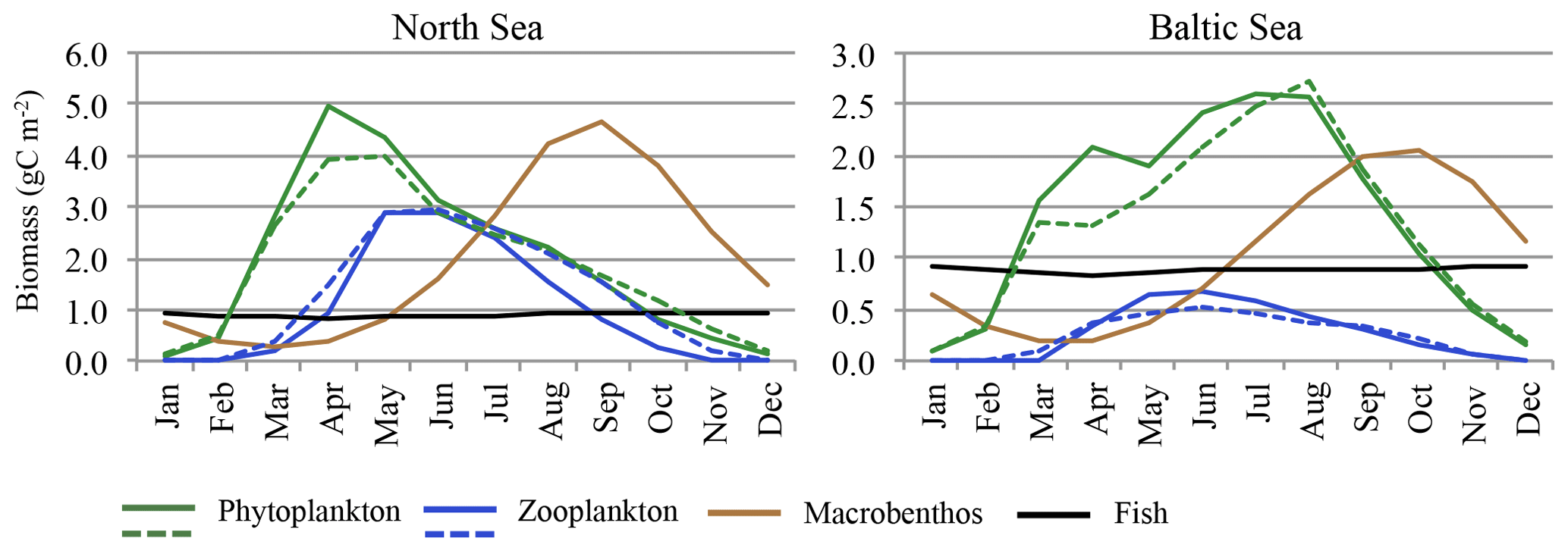
Figure 4 Average seasonality of ecosystem components. Monthly means averaged for 1980–1989. Solid lines represent ECOSMO E2E, and dashed lines represent ECOSMO II (phytoplankton and zooplankton).

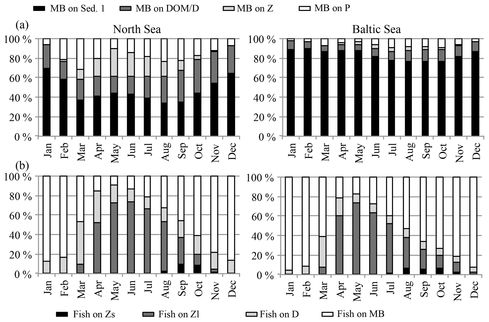
Figure 5 Prey composition of (a) macrobenthos (MB) and (b) fish in the North Sea (left) and the Baltic Sea (right). MB feeds on Sed. 1 (organic material in the sediment), DOM ∕ D (dead organic material in the water column; dissolved organic matter ∕ detritus), Z (zooplankton), and P (phytoplankton). Fish feed on Z_s (“small” herbivorous zooplankton), Z_l (“large” omnivorous zooplankton), D (detritus), and MB.

3.2 Seasonal dynamics of ecosystem components and diet composition

Values for both MB and fish biomass vary over the course of the year (Fig. 4). While the modelled seasonal amplitude for fish biomass is relatively small (94.7 mg C m⁻³ ≅ 11 % of the mean biomass in the North Sea and 84.8 mg C m⁻³ ≅ 9.7 % of the mean biomass in the Baltic Sea) when compared to the average values, MB seasonality is substantial (4.4 g C m⁻³ ≅ 222 % of the mean biomass in the North Sea and 1.86 g C m⁻³ ≅ 183 % of the mean biomass in the Baltic Sea). Minimum MB and fish biomass is estimated for winter and early spring, and the seasonal maximum is modelled for late summer and autumn. The MB maximum lags behind the zooplankton maximum by about 3 months. In contrast to zooplankton, the MB minimum does not reach values close to zero; however, the model also simulates a significant standing stock for MB during winter.

In Fig. 4 the seasonal cycles for the phytoplankton and zooplankton estimates of the ECOSMO E2E run are presented along with those of the ECOSMO II simulation (Daewel and Schrum, 2013). The seasonal cycles for both phytoplankton and zooplankton are clearly affected by the consideration of MB and fish. Although the general phytoplankton biomass seasonality and the phenology remain relatively unchanged, the magnitude of the seasonal maximum, especially of the diatom bloom, is significantly increased in spring and early summer in both the North Sea and Baltic Sea regions when the MB and fish groups are included. The consideration of seasonally variable MB and fish predation on zooplankton imposes a different seasonality on zooplankton mortality compared with the constant mortality rate used in ECOSMO II (Daewel and Schrum, 2013) and therefore impacts zooplankton phenology. The reduced zooplankton biomass at the beginning of the season due to MB and fish predation (Fig. 5) consequently leads to a reduction in phytoplankton mortality and an increase in phytoplankton biomass (top-down process). Additionally, MB competes with zooplankton for resources and thereby changes zooplankton seasonality, especially in autumn in the North Sea when MB biomass is highest and it preys dominantly on dead organic material and phytoplankton (Fig. 5).

An overview of the seasonal feeding dynamics can be obtained by identifying the monthly prey composition for MB (Fig. 5a) and fish (Fig. 5b) in the North Sea and the Baltic Sea. For MB, the major food source throughout the year is organic sediments followed by dead organic material, although the percentage of the latter is considerably higher in the North Sea than in the Baltic Sea, presumably due to the fact that a higher percentage of detritus is resuspended in the tidally influenced, highly turbulent areas of the North Sea. Zooplankton and phytoplankton are included in the MB diet when available in spring and summer. The fish prey composition (Fig. 5b) is very similar in both sub-areas: MB dominates the diet in the autumn and winter months and omnivorous (large) zooplankton dominates in summer. Detritus contributes a significant food source in March and April, while small zooplankton only appears in autumn and in very low amounts. Greenstreet et al. (1997) reviewed food web studies in the North Sea and analysed the food consumption of fish by guild. When adding up the average MB and zooplankton in the diet of the four fish guilds considered in the study (demersal piscivores, demersal benthivores, pelagic piscivores, and pelagic planktivores), the zooplankton ∕ MB ratio in the diet lies at around 6 ∕ 4 in summer, which is comparable to our estimated food composition in summer. In contrast to our model results, the estimates from Greenstreet et al. (1997) show no significant seasonal variations in diet composition. Explanations for this disagreement might be found in the model performance of e.g. the zooplankton standing stock. The latter has been estimated to be very low in winter, and hence lead to an intensification of the modelled zooplankton seasonal cycle and to too little zooplankton in the fish diet in winter. Another possible reason for the mismatch between the model and the estimates from Greenstreet et al. (1997) might be related to spatio-temporal differences in the fish biomass and diet.

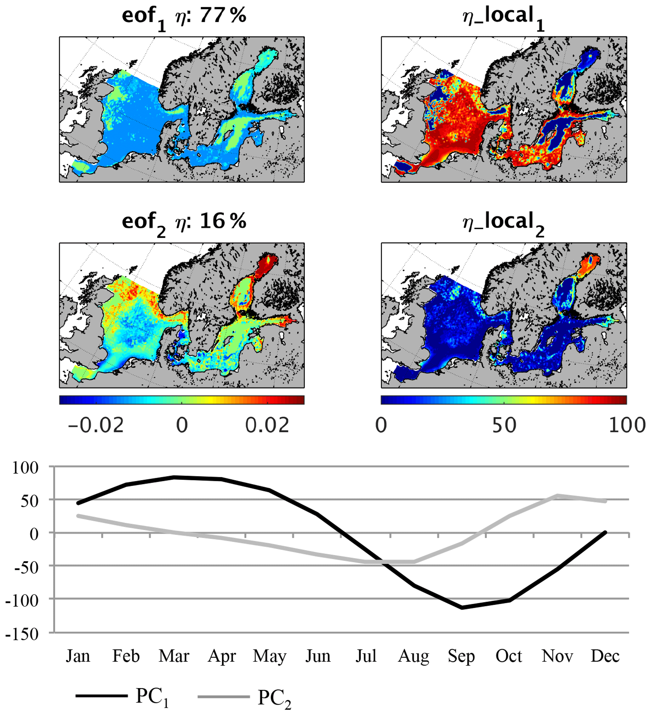
Figure 6 Empirical orthogonal function (EOF) of macrobenthos biomass average seasonality (1980–1989). eof_1,2 refers to the spatial pattern of the first and second EOF mode; η refers to the global explained variance; η_local refers to the local explained variance for the first and second EOF; PC_1,2 refers to the temporal variability related to eof_1,2.

Figure 7 Empirical orthogonal function (EOF) of fish biomass average seasonality (1980–1989). eof_1,2 refers to the spatial pattern of the first and second EOF mode; η refers to the global explained variance; η_local refers to the local explained variance for the first and second EOF; PC_1,2 refers to the temporal variability related to eof_1,2.

An EOF analysis of the monthly mean fields for MB and fish biomass reveals the spatial–seasonal pattern. In Fig. 6 (MB) and Fig. 7 (fish) the first two EOF patterns are shown for MB and fish biomass respectively. Additionally, the local explained variance and the related temporal pattern (PC) are given. For MB, the seasonal signal is very homogeneous across the whole area (Fig. 6). The first mode explains a significantly large part – 77 % – of the overall variability, and the temporal signal resembles the average variability shown in Fig. 4. This highlights that the MB seasonality is mainly induced by the seasonal pattern of the system productivity with increased production of fresh organic material in summer and less food availability in winter. This is in line with observations on the seasonality of benthic infauna at three different locations in the North Sea published by Reiss and Krönke (2005), who found maximum biomass in late summer. Although the observed seasonality showed the highest magnitude in the German Bight, the seasonality was clear at all three locations. The authors concluded that of the potential relevant factors (food availability/quality, water temperature, predation, and hydrodynamic stress), food quality plays the major role for infauna seasonality; thus, this factor is strongly related to primary production. They also suggest food limitation and predation pressure to be the main processes influencing the decrease in abundance during winter. Furthermore, the same authors looked at seasonality in the epibenthic community (Reiss and Krönke, 2004) and showed that the epifaunal biomass varies less seasonally, especially in the offshore region, and that the main processes causing seasonal variations are related to migratory behaviour, which is not covered by our model. For the Baltic Sea only, very local studies in seasonality of MB are available with some of these indicating strong local seasonality (Anders and Möller, 1983); however, in other regions no seasonal changes in biomass were observed due to the dominance of long-lived species (Persson, 1983). On the one hand, the comparison with observations generally indicates that the model is able to represent the main seasonality in MB even though epifauna and infauna are not separated. On the other hand, in future studies the consideration of an additional functional group encompassing longer-lived species will be required to more correctly address MB seasonality.

The second EOF explains about 16 % of the overall variability and is especially important in the Gulf of Finland and Bothnian Bay where it explains to up to 80 % of the total variability. PC₂ differs from PC₁ by showing a maximum in MB in late autumn and winter with a time lag of about 2 months compared with PC₁, whereas the minimum is modelled for July and August. The ecosystem seasonality in the Bothnian Bay and the Gulf of Finland is highly impacted by a relatively long period of winter sea ice cover; therefore, the onset of the spring bloom is delayed (see e.g. Andersson et al., 1996; Daewel and Schrum, 2013). This would consequently affect the phenology of MB and fish in that area and explains the difference in the seasonal cycle.

In contrast to the MB pattern, the EOF of the fish biomass seasonality (Fig. 7) reveals a clear distinction between seasonal signals in different regions. Together, the first two EOFs explain over 70 % of the overall variability, whereas the first EOF comprises 44 %. This first pattern describes a seasonal cycle with a minimum in March/April and a plateau in maximum fish production between August and December, which dominates the average seasonal cycle shown in Fig. 4. It specifically explains the seasonality in the deeper central North Sea, the Norwegian Trench, the Skagerrak, and the northern Kattegat region as well as the coastal areas of the central Baltic basins. In all of these regions this mode explains up to 80 % of the variability. The second pattern describes the seasonal variability in the shallow areas of the southern North Sea, including Dogger Bank, the north-western North Sea, and the belts at the entrance to the Baltic Sea, with a maximum in fish biomass in late spring and summer. The dynamics in these areas are determined by the zooplankton seasonality featuring a maximum in summer, which is unlike the central North Sea. The two modes of the estimated fish seasonal cycles clearly indicate two different fish habitats, structured by food availability and temperature. In Fig. 8, fish production, partitioned into diet components, in the shallow (Fig. 8a) and deeper (Fig. 8b) North Sea is illustrated along with the seasonal temperature cycle. The main differences contributing to variations in fish biomass seasonality are the timing of the food resources and the difference in temperature. In the shallow areas of the North Sea, zooplankton forms the major food source for fish in early spring and summer, reaching a maximum in May and June. Following this, the MB contribution increases and resumes its role as the major food source in August. In the deeper parts of the North Sea, the dynamics of the fish diet composition are shifted by 1–2 months, and, in contrast to the shallower North Sea, dead organic material plays an important role throughout the year. As the seasonality in total fish production is very similar in both regions, this difference in diet composition would not inherently lead to a difference in fish biomass seasonality, as seen from the EOF analysis (Fig. 7). However, in addition to the difference in food resources, the two habitats feature very different seasonal temperature cycles. The most likely explanation for the stronger decrease in fish biomass in the shallow North Sea in August and September (Fig. 7, PC₂) is the temperature-driven higher loss rate (Eq. 11).

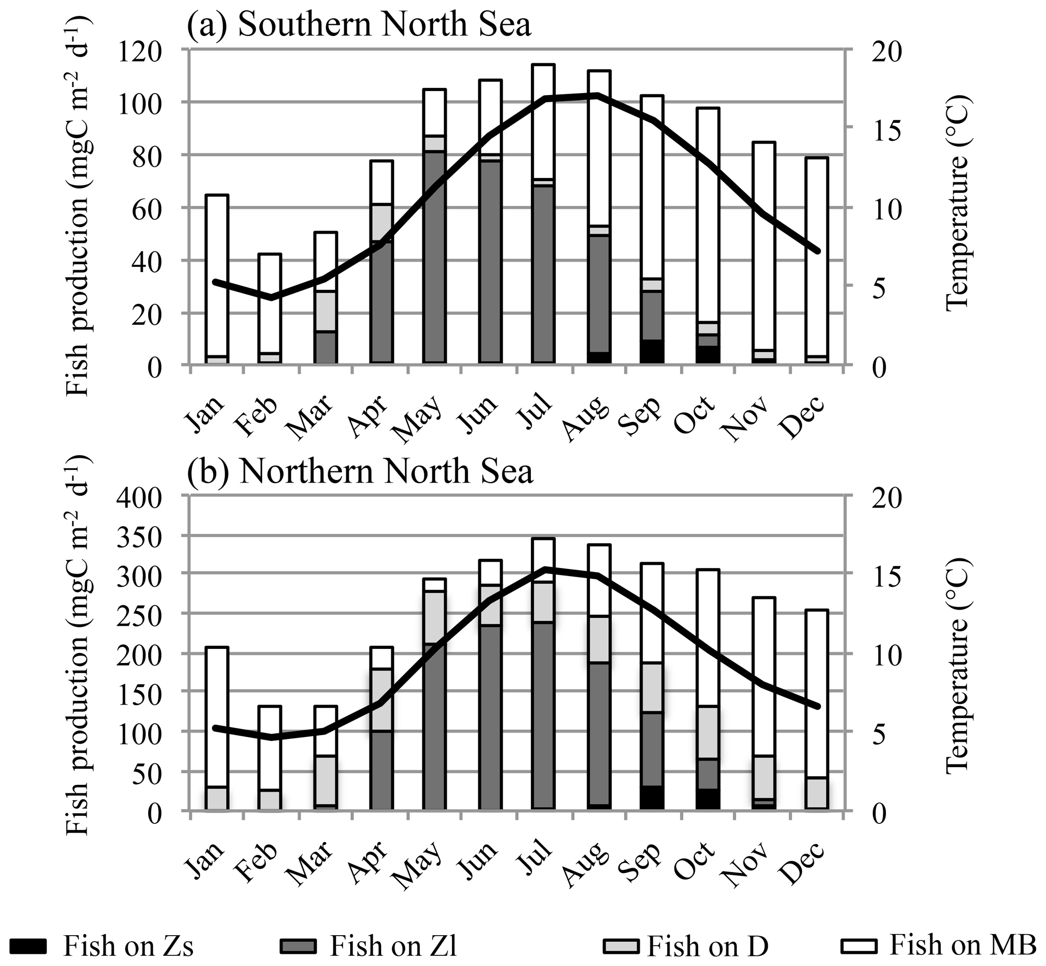
Figure 8 Seasonal cycle of fish production (primary y axis) in the shallow (depth < 50 m) southern North Sea (a) and in the deeper (depth > 50 m) northern North Sea (b), divided into diet components (Z_s denotes herbivorous zooplankton; Z_l denotes omnivorous zooplankton; D denotes detritus; MB denotes macrobenthos). The mean depth averaged temperature in the respective region is also shown (solid line; secondary y axis).

Here, we can identify the distinction of North Sea fish communities at approximately the 50 m depth line, which is comparable to the separation line reported for North Sea fish communities in earlier published observational studies (Callaway et al., 2002; Rees et al., 1999). Using data from 270 stations distributed over the whole North Sea, Callaway et al. (2002) separated the North Sea fish community into several clusters (three or five in depending on the trawling method) and two main groups. The most conspicuous boundary was defined at approximately the 50 m depth contour separating the community in the shallow southern North Sea, which mainly consisted of small non-commercial species, from the community in the central North Sea, which was dominated by haddock (Melanogrammus aeglefinus), Merlangius merlangus, herring (Clupea harengus), and plaice (Pleuronectes platessa). The authors also suggested that the environmental conditions in the region play a major role in structuring the community. Although our model cannot distinguish between different species and actual communities, the results indicate a clear distinction between the seasonality and the driving environmental conditions of fish production potential in the shallow southern North Sea and in the central North Sea.

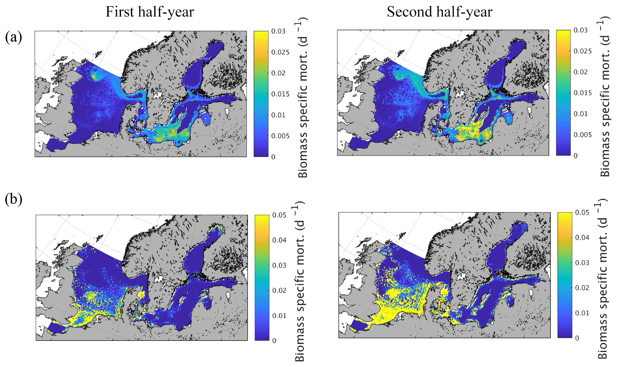
Figure 9 Semi-annually averaged (1980–1989) biomass-specific mortality (d⁻¹) of zooplankton due to (a) fish predation and (b) macrobenthos predation.

Spatial variations of biomass-specific mortality related to zooplankton consumption by fish and MB are given in Fig. 9 as an average from 1980 to 1989. The results were additionally separated into the first and second quarter of the year to identify potential intra-annual variations as suggested by Maar et al. (2014). The results show a very distinct spatial pattern for fish-induced zooplankton mortality (Fig. 9a) with increased values in some specific regions in the central North Sea, especially in the vicinity of Dogger Bank, close to the English coast, Oyster Ground, and in the Fisher Bank (Little and Great Fisher Bank) area. Furthermore, our model shows considerable consumption in the Norwegian Trench, along the coast of the southern and central Baltic Sea including the Kattegat/Skagerrak region, in the central basins of the southern Baltic Proper, the Gulf of Gdansk, and in the Gulf of Riga. The biomass-specific mortality related to MB consumption (Fig. 9b), in contrast, is confined to shallow areas with a relatively strong coupling between the benthic and pelagic system. This includes the shallower areas of the southern and central North Sea and the near coastal areas in the Baltic Sea. The difference between the first half and the second half of the year is relatively small for the fish-induced mortality. However, there is a clear but small increase in the central North Sea and a much stronger change in the Baltic Sea pattern with a higher impact in the second half of the year. For MB the impact is substantially stronger for the second half of the year, which is clearly related to the strong seasonal signal in MB biomass.

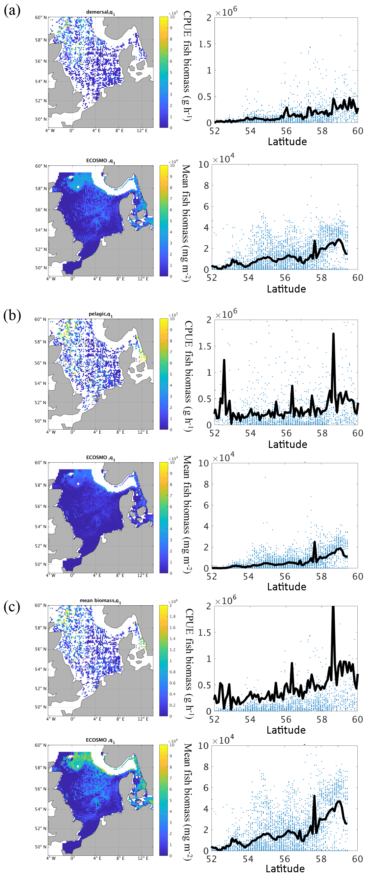
Figure 10 (a–c) Mean (1980–1989) total fish biomass from the ICES IBTS survey and fish biomass from ECOSMO E2E for the associated sampling time and area in the first quarter of the year (January–March) for demersal species (a), pelagic species (b), and combined biomass (c). Left panels show the spatial distribution of fish biomass. Right panels show the biomass versus latitude and the mean of biomass at latitude (black line).

While we estimate zooplankton predation losses within the model, an earlier study by Maar et al. (2014) proposed spatial–temporal variations in biomass-specific mortality of zooplankton based on data of the major zooplanktivorous fish species and on larval distribution in the North Sea (their Fig. 10c, d). Our results show clear similarities in magnitude and spatial structure when compared to the results from Maar et al. (2014). However, the results of Maar et al. (2014) showed a clear difference between the first half of the year and the second half of the year with decreased biomass-specific mortality in the second half of the year in the central North Sea. This intra-annual variation is not evident in our model results. Nevertheless, we found a clear difference in magnitude when comparing winter and summer season (not shown). The reasons for the discrepancies between our model results and Maar et al. (2014) are presumably related to inter-annual variations in fish consumption (which are not considered in a 10-year average) the fact that migration is not considered in the model and thus restrict the spatial variation, and that our functional group cannot resolve species- and stage-specific spatial and temporal variations such as the increase in larval biomass in spring and changes in species composition. Conversely, the approach from Maar et al. (2014) reveals uncertainties due to the fact that only parts of the North Sea fish assemblage are considered and that the fish biomass is prescribed and not dynamically coupled to zooplankton biomass.

The approach from Maar et al. (2014) provides the possibility of replacing the spatially and temporally invariant closure term usually used in NPZD-type models (Daewel et al., 2014) with a data-driven, detailed formulation, and allows for the consideration of the predation effects of different fish species and larvae on the zooplankton dynamics. However, the main disadvantage is that, as the authors already pointed out, a huge amount of detailed species specific and potentially under-sampled data are required and that the estimated mortality index relies on a number of assumptions concerning factors such as the relevance of the individual fish species and spawning time and distribution. Moreover, such a data-driven approach has a limited potential for future projections and sensitivity studies regarding various effects on the ecosystem. However, following a very different, less detailed approach, the spatial variability of our estimates of zooplankton consumption (Fig. 9a) by fish compares surprisingly well to the spatial variability of the fish consumption index provided by Maar et al. (2014; their Fig. 4), which we consider to be an implicit validation of our model approach. The consideration of MB-related zooplankton predation mortality is an additional advantage that arises from our modelling approach.

Figure 11 Taylor diagram for surface (< 10 m) nutrients (model versus ICES data) in different areas of the North Sea (area separation in ICES boxes according to Fig. 1), showing nitrate (a) and phosphate (b). Arrows indicate regions with relatively large changes in the validation measures.

3.3 Model performance and nutrient dynamics

To get a more direct measure of the validity of the modelled fish functional group we used data from the NS-IBTS. In Fig. 10, we compared the mean fish functional group biomass distribution to the fish biomass from the NS-IBTS calculated following the method described in Sect. 2.3. We classified species within the North Sea fish community into “demersal” (Fig. 10a) and “pelagic” groups (Fig. 10b) based on life-history characteristics, and then summed the biomass of each group to form a “combined” (Fig. 10c) group. In contrast to the species-specific differentiation into groups used for the observations, the model results do not provide this level of detail. Here, the differentiation was performed based on the vertical distribution of the fish biomass. Thus, we assigned all biomass in the bottom layer to the “demersal” groups and biomass in the remaining water column to the “pelagic” group. Therefore, and because the units in the NS-IBTS data and in the model data differ, the figures are not quantitatively comparable. When we compare the data for the different fish groups we find that the “demersal” fish increase more strongly with latitude and (following the North Sea bathymetry) with depth. The “pelagic” fish group biomass, in contrast, shows, in addition to the increase with latitude, a maximum in the south and in the north of the North Sea. In general, we find a clear increase in fish biomass with latitude with a maximum at the entrance to the North Sea, but also higher values in the central North Sea and around Dogger Bank. From the data, we can also conclude that the contribution of pelagic fish biomass to the overall biomass is higher in the south than further north. From a purely qualitative comparison, we find that the modelled fish group biomass roughly resembles the observed pattern, with increasing biomass from south to north. The model also represents the maximum in the Kattegat and at the northern shelf edge. However, the model estimates a pronounced minimum off the British coast, which is not evident from the observations; this likely stems from the zero boundary condition, meaning that no fish enters or leaves the model area over the lateral boundaries, and the missing migration parameterization in the model. In summary, we found that the model is able to represent the spatial fish distribution in the North Sea. However, the differences in fish biomass off the British and partly at the European continental coast in addition to the discrepancy between the observed and modelled “pelagic” group indicate a potential under-representation of the pelagic fish stock by the simulated fish functional group.

To understand the effect of changes in the NPZD model closure on model performance with respect to nutrient dynamics, we repeated the nutrient validation for surface nutrients in the North Sea (Fig. 11) and for nutrient profiles in the Baltic Sea (Fig. 12) as described by Daewel and Schrum (2013). For both surface nitrate (Fig. 11a) and phosphate (Fig. 11b) the statistics, presented here using a Taylor diagram, indicate an improvement for some regions when MB and fish are considered. Larger improvements occur in regions with relatively high estimated biomass for MB and fish, such as in region E off the English coast, where the correlation coefficient for nitrate improved from under 0.4 to 0.5, and for phosphate from under 0.6 to above 0.7, although with a stronger bias for both nutrients. Better results were also accomplished in the central North Sea (region K), where the standard deviation moved significantly closer to that of the observations. Small improvements are also shown for regions F and L.

The MB and fish groups potentially alter the nutrient dynamics in the Baltic Sea (Fig. 12). Although we found only relatively small changes for phosphate compared with the ECOSMO II simulation in both locations considered, clear differences for the nitrogen and oxygen profiles were apparent, especially in the intermediate depth levels between 50 and 150 m and at the surface. The model indicates a slight upward shift of the oxycline when fish and MB are resolved, which also affects nitrate by relocating the nitrate maximum. This results in decreased model performance with respect to nitrate in the intermediate layer, but improves the performance at the surface by increasing the initially (too) low modelled surface nutrient concentrations. Ammonium is significantly improved in lower layers at the BY15 station for the ECOSMO E2E model. Several processes interact to determine the changes in vertical nutrient profiles. Examples of possible candidates are as follows: changes in the oxygen dynamics due to including oxygen dependent fish and MB, and changes in sediment dynamics, as organic sediments are ingested by MB and nutrients are subsequently released on different time and spatial scales. Additionally, we found that the nutrient dynamics are also sensitive to the parameter choice of zooplankton mortality and the loss rate though fisheries and apex predation (cf. Sect. 3.4).

Figure 12 Modelled (blue: ECOSMO II; green ECOSMO E2E) and observed (HELCOM data: black) vertical nutrient profiles. Data were averaged over the 10-year period from 1980 to 1989 and the mean (full line) and standard deviation (dashed line) are presented at two distinct locations in the Baltic Sea, BY15 (a) and BY05 (b) (see Fig. 1).

4 Ecosystem response to structuring drivers

Using the two sets of scenarios, we try to evaluate the impact of changes in model closure (fisheries mortality) and zooplankton mortality on ecosystem structure.

In the fisheries scenarios we would expect a top-down response of the ecosystem dynamics to changes in fisheries, such that reduced fish biomass would relax the predation on the secondary producers (zooplankton and MB), which would consequently increase the biomass and reduce the phytoplankton (see e.g. Cury et al., 2003). Our model results indicate this type of trophic response for the Baltic Sea ecosystem (Fig. 13b), but with very little efficiency for the lowest trophic level. The reduction of fish biomass for the highest catch rate scenario is about 98 % compared with the control run, and for zooplankton and MB the increase is 13 % and 62 % respectively. The response of phytoplankton biomass, in contrast, is only of the order of 4 % and is therefore small compared to the inter-annual variability of phytoplankton biomass, which is of the order of 10 %.

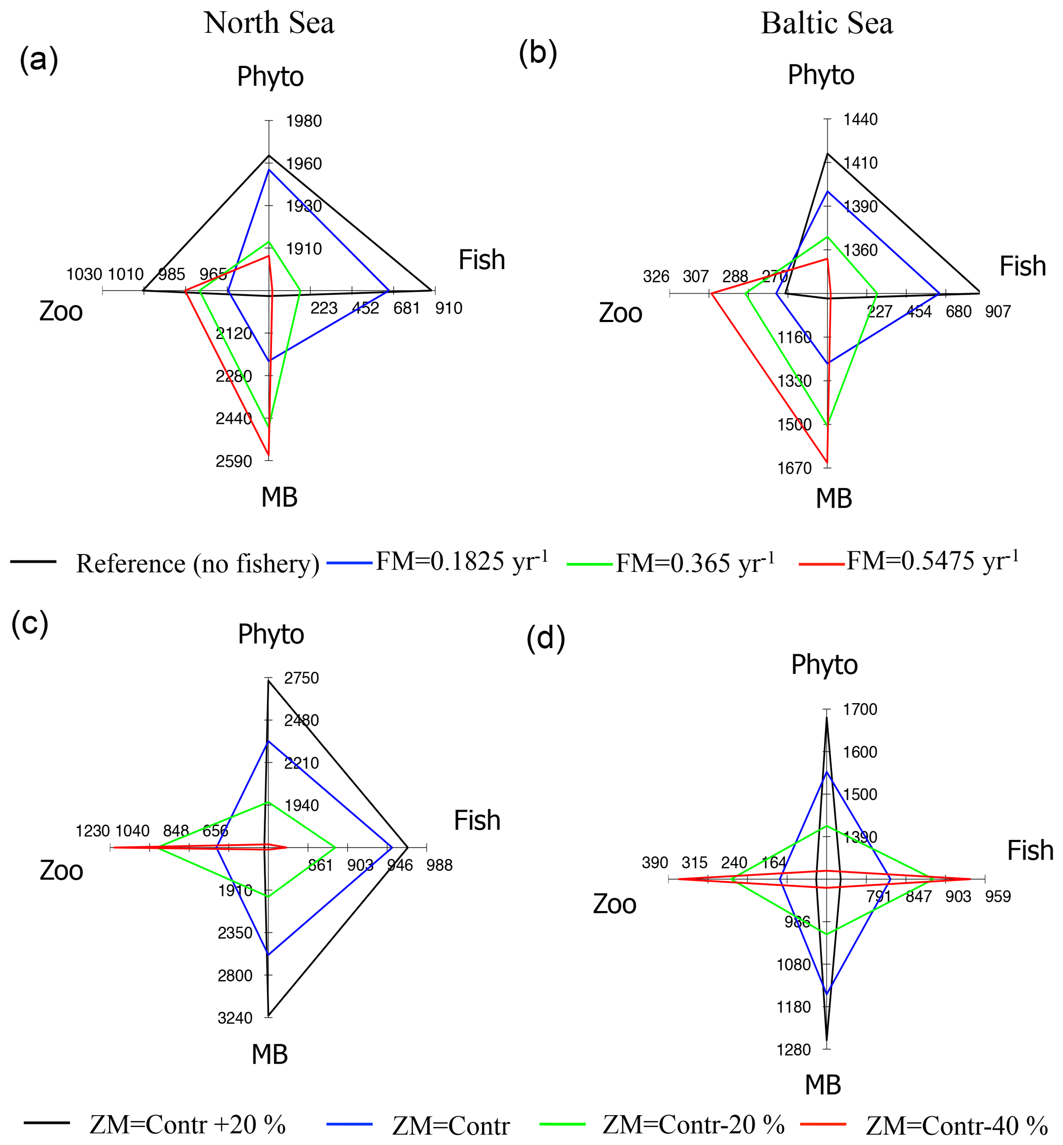
Figure 13 Spider chart showing averaged changes in North Sea and Baltic Sea annual mean phytoplankton (Phyto), zooplankton (Zoo), MB, and fish biomass (mg C m⁻²) due to specific changes in the food web components. (a, b) Scenarios for fisheries mortality (FM); (c, d) scenarios for changes in zooplankton natural mortality (ZM).

The North Sea ecosystem responds less predictably than the Baltic Sea to simulated changes in the fish model closure term. Although the reduction of fish biomass in the North Sea results in an increase in MB, zooplankton biomass does not respond in the same fashion (Fig. 13a). The introduction of a moderate loss term leads to a comparably strong reduction of zooplankton biomass, while, with further increase in the loss rate zooplankton biomass increases again. As in the Baltic Sea, phytoplankton biomass is reduced with increasing fishing effort but the response is even smaller (∼ 3 %). The most likely reason for the more complex response of the North Sea ecosystem is the tighter coupling between MB and zooplankton and phytoplankton (see Fig. 7a). As zooplankton forms a prey group for MB in the North Sea, a major change in MB and fish biomass affects the relevance of the two zooplankton predator groups and the increased predation pressure by MB will counteract (and potentially overshadow) the relaxed predation by fish.

The second set of scenario experiments was designed to understand the ecosystem response to changes in the zooplankton natural mortality. In the new E2E model configuration a change in this term cascades up and down the trophic food chain (Fig. 13c, d). In both systems, a reduction in zooplankton natural mortality subsequently leads to an increase in zooplankton biomass and to a decrease in phytoplankton as well as an associated decrease in MB. The difference between the systems becomes manifest in the response of the fish group, which is positive in the Baltic Sea (Fig. 13d), but reverses in the North Sea (Fig. 13c) with higher fish biomass in a low zooplankton environment. This response once again highlights the major role of MB in the North Sea ecosystem, which partly competes with zooplankton and forms a major prey item for fish.

Despite the strong changes in the magnitude of phytoplankton and zooplankton biomass, the phenology of the seasonal cycles was almost not impacted by the sensitivity changes (not shown). The only distinct change is a decrease in phytoplankton spring biomass in the Baltic Sea when the model closure term is increased. Almost none of the other phenological changes described in Sect. 3.2 were affected when fish biomass was decreased in the first set of sensitivity experiments, highlighting the dominant role of MB in these changes.

5 Conclusion

In this study, we presented a 3-D resolved food web model that is based on a functional group approach ranging from nutrients to fish. In contrast to the study by Fennel (2010), we did not distinguish between different fish species to avoid the uncertainties associated with the choice of fish species and their contribution, compared with the unconsidered remaining biomass. Our approach integrates the full production potential for fish into one single functional group by defining the feeding pathways via primary and secondary production, including zooplankton and MB. This approach has certain advantages. For example, we avoid the parameterization of a detailed species dependent food web, and the adaptability of the model to other ecosystems is independent of the local fish assemblage. The advantage of the generic functional group approach used in the model for all trophic levels is that we can simplify a complex community structure and reduce the information to the basic common features, thereby avoiding a huge parameter set and excessive data requirements. Still the model is able to simulate relevant ecosystem dynamics at high spatial and temporal resolutions with relatively low computational requirements.

Despite the simplicity of the approach, we found that the model was able to reproduce the observed spatial pattern and magnitude of both macrobenthos and fish biomass in the North Sea and the Baltic Sea as described in the literature (see Fig. 3 and Sect. 3.1). This highlights the advantage of our approach, and adds weight to the assumption that the fish biomass distribution consequently emerges from prey availability and environmental conditions. Furthermore, the model was able to distinguish between the two different fish production areas, which were separated around the 50 m depth line (compare Callaway et al., 2002), with differences in the seasonal cycle and the diet composition. Although this differentiation is not based on species composition as in Callaway et al. (2002), it shows the basic concept that biotic and abiotic conditions determine the composition of the local fish community, as realised in the model, and allows for conclusions to be formed about the local fish community, even when it is not explicitly prescribed in the model. This opens up possibilities for additional investigations on topics such as the inter-annual variability of fish production and biomass through general fish diet composition, as well as investigations on how this compares to observed long-term fish stock variations. Future model developments and applications should particularly address the composition of local fish communities, by classifying fish into two or more functional groups such as planktivores and piscivores, or into pelagic and benthic feeding guilds, to allow for a clearer representation of the food web structure.

However, the simplicity of the model and the related assumptions confine the model interpretation, and some of the simplifications require revision in future model applications. Besides the redistribution of the MB and fish into several food web-specific functional groups, neglecting fish movements in the model approach is a clear limitation, as we know that fish are mobile and would migrate in response to factors including food shortage, spawning behaviour, or predators. In contrast to the Norwegian Sea, where distinct feeding migrations are observed for the pelagic fish component (Nøttestad et al., 2011) following the northward progressing zooplankton blooms and light conditions, the North Sea and the Baltic Sea exhibit a relatively constant spatial pattern of system productivity, with highly productive areas along the coast and less productivity in the central seasonally stratified regions. Hence, the migratory movements of North Sea and Baltic Sea fish stocks might not be based solely on large feeding migrations, but may also related to temperature and salinity changes and spawning behaviour (Hinrichsen et al., 2016; Hunter et al., 2003; Pinto et al., 2018; Radtke et al., 2013). Additionally, fish migrate into the area from the North Atlantic (e.g. Sparholt, 1990). Two questions arise that are specifically related to this topic: (i) Is including migration strategies on a functional group level effective and reasonable in the North Sea and the Baltic Sea environment, considering the variability among species? (ii) Would migration behaviour effectively impact the productivity of the system at the higher trophic level? Therefore, we would like to highlight the necessity of investigating the impact of specific migration strategies in continuative studies.

One major aim of the model development was to solve the closure term problem that arises with NPZD-type models when choosing a fixed zooplankton mortality term (for review see Daewel et al., 2014). The model results show that the inclusion of a higher trophic functional group can provide a more consistent and dynamic closure term, which produces a realistic but variable mortality field independent of in situ observations, in contrast to observational-based zooplankton predation as used by studies such as Maar et al. (2014). In return, the closure term problem is transferred to the new “end” of the food web, namely the fish group mortality. In future studies, this should be addressed by including dynamic formulations for apex predators and fisheries. This might be accomplished by introducing simple fisheries catch rates as explored in the scenario runs in this study (Sect. 3.4), or by coupling the model to socio-economic models, which allow for the inclusion of social interests and management decisions in the modelling approach (e.g. Charles, 1989; Schlüter et al., 2014). The latter approach could allow the model to be applied in a fisheries management context if the model's ability to capture local fish community structure with respect to potential production and species composition was further developed.