Discrete k-nearest neighbor resampling for simulating multisite precipitation occurrence and model adaption to climate change

Stochastic weather simulation models are commonly employed in water resources management, agricultural applications, forest management, transportation management, and recreational activities. Stochastic simulation of multisite precipitation occurrence is a challenge because of its intermittent characteristics as well as spatial and temporal cross-correlation. This study proposes a novel simulation method for multisite precipitation occurrence employing a nonparametric technique, the discrete version of the k-nearest neighbor resampling (KNNR), and couples it with a genetic algorithm (GA). Its modification for the study of climatic change adaptation is also tested. The datasets simulated from both the discrete KNNR (DKNNR) model and an existing traditional model were evaluated using a number of statistics, such as occurrence and transition probabilities, as well as temporal and spatial cross-correlations. Results showed that the proposed DKNNR model with GA-simulated multisite precipitation occurrence preserved the lagged cross-correlation between sites, while the existing conventional model was not able to reproduce lagged cross-correlation between stations, so long stochastic simulation was required. Also, the GA mixing process provided a number of new patterns that were different from observations, which was not feasible with the sole DKNNR model. When climate change was considered, the model performed satisfactorily, but further improvement is required to more accurately simulate specific variations of the occurrence probability.

1 Introduction

Stochastic simulation of weather variables has been employed for water resources management, hydrological design, agricultural irrigation, forest management, transportation planning and evacuation, recreation activities, filling in missing historical data, simulating data, extending observed records, and simulating different weather conditions. Stochastic simulation models play a key role in producing weather sequences, while preserving the statistical characteristics of observed data. A number of stochastic weather simulation models have been developed using parametric and nonparametric approaches (Lee, 2017; Lee et al., 2012; Wilby et al., 2003; Wilks, 1999; Wilks and Wilby, 1999).

Parametric approaches simulate statistical characteristics of observed weather data with a set of parameters that are determined by fitting (Jeong et al., 2012; Lee, 2016; Zheng and Katz, 2008), whereas in nonparametric approaches, historical analogs with current conditions are searched, following the weather simulation data (Buishand and Brandsma, 2001; Lee et al., 2012). Combinations of parametric and nonparametric approaches have also been proposed (Apipattanavis et al., 2007; Frost et al., 2011).

Among weather variables, precipitation possesses intermittency and zero values between precipitation events, which make it difficult to properly reproduce the events (Beersma and Buishand, 2003; Hughes et al., 1999; Katz and Zheng, 1999). To overcome the problem of intermittency and zero values, precipitation is simulated separately from other variables. The main method for reproducing intermittency has been the multiplication of precipitation occurrence and an amount as $Z=X\cdot Y$, where X is the occurrence (binary as either 0 or 1) and Y is the amount (Jeong et al., 2013; Lee and Park, 2017; Todorovic and Woolhiser, 1975). The spatial and temporal dependence in the occurrence and amount of precipitation introduce further complexity in multisite simulation.

Wilks (1998) presented a multisite simulation model for the occurrence process (i.e., X) using the standard normal variable that is spatially dependent, representing the relationship between the occurrence variable and the standard normal variable with simulation data. Originally, the occurrence of precipitation had been simulated with a discrete Markov chain (MC) model (Katz, 1977). Compared to the MC model that requires a significant number of parameters for generating multisite occurrence, the multisite occurrence model proposed by Wilks (1998) transforms the standard normal variate and simulates the sequence with multivariate normal distribution, and then back-transforms the multivariate normal sequence to the original domain. The model is able to reproduce the contemporaneous multisite dependence structure and lagged dependence only for the same site but it requires a complex simulation process to estimate parameters for each site and is unable to preserve lagged dependence between sites. Also, a recent improvement has also been made, but the weakness of the model in Wilks (1998) was not significantly improved (Evin et al., 2018; Mehrotra et al., 2006; Srikanthan and Pegram, 2009).

Lee et al. (2010) proposed a nonparametric-based stochastic simulation model for hydrometeorological variables. Their model overcame the shortcomings of a previous nonparametric simulation model (Lall and Sharma, 1996), called k-nearest neighbor resampling (KNNR), but the simulated data do not produce patterns different from those of the observed data (Brandsma and Buishand, 1998; Mehrotra et al., 2006; St-Hilaire et al., 2012). In addition to KNNR, Lee et al. (2010) used a metaheuristic genetic algorithm (GA) that led to the reproduction of similar populations by mixing the simulated datasets. Note that the reproduction procedure of the GA allows to generate new patterns that are similar to observed patterns, but a small number of totally new patterns are simulated from the mutation procedure of the GA.

While KNNR is employed to find historical analogues of multisite occurrence similar to the current status of a simulation series, GA is applied to use its skill to generate a new descendant from the historical parent chosen with the KNNR. In this procedure, the multisite occurrence of precipitation can be simulated while preserving spatial and temporal correlations. Metaheuristic techniques, such as GA, have been popularly employed in a number of hydrometeorological applications (Chau, 2017; Fotovatikhah et al., 2018; Taormina et al., 2015; Wang et al., 2013). Although a number of variants of KNNR-GA have been applied (Lee et al., 2012; Lee and Park, 2017), none of them can simulate multisite occurrence of precipitation whose characteristics are binary and temporally and spatially related.

Therefore, this study proposes a stochastic simulation method for multisite occurrence of precipitation with the KNNR-GA-based nonparametric approach that (1) simulates multisite occurrence with a simple and direct procedure without parameterization of all the required occurrence probabilities, and (2) reproduces the complex temporal and spatial correlation between stations, as well as the basic occurrence probabilities. The proposed nonparametric model is compared with the popular model proposed by Wilks (1998). Even though the multisite occurrence data generated from the Wilks model preserves various statistical characteristics of the observed data well, significant underestimation of lagged cross-correlation still exists. Furthermore, the relation between standard normal variable and occurrence variable relies on long stochastic simulation.

The paper is organized as follows. The next section presents the mathematical background of existing multisite occurrence modeling and section discusses the modeling procedure. The study area and data are reported in Sect. 4. The model application is presented in Sect. 5. Results of the proposed model are discussed in Sect. 6, and summary and conclusions are presented in Sect. 7.

2 Background

2.1 Single site occurrence modeling

Let $X_t^s$ represent the occurrence of daily precipitation for a location s ($s=\mathrm{1},\mathrm{\dots },S$) on day t ($t=\mathrm{1},\mathrm{\dots },n$; n is the number observed days) and let $X_t^s$ be either 0 for dry days or 1 for wet days. The first-order Markov chain model for $X_t^s$ is defined with the assumption that the occurrence probability of a wet day is fully defined by the previous day as

$$\begin{array}{}\text{(1)}& {\displaystyle }& {\displaystyle }\mathrm{Pr}\left\{X_t^s=\mathrm{1}\mathrm{|}{X}_{t-\mathrm{1}}^s=\mathrm{0}\right\}=p_{\mathrm{01}}^s\text{(2)}& {\displaystyle }& {\displaystyle }\mathrm{Pr}\left\{X_t^s=\mathrm{1}\mathrm{|}{X}_{t-\mathrm{1}}^s=\mathrm{1}\right\}=p_{\mathrm{11}}^s.\end{array}$$

Also, $p_{\mathrm{00}}^s=\mathrm{1}-p_{\mathrm{01}}^s$ and $p_{\mathrm{10}}^s=\mathrm{1}-p_{\mathrm{11}}^s$, since the summation of 0 and 1 should be unity with the same previous condition. This consists of a transition probability matrix (TPM) as

$$\begin{array}{}\text{(3)}& {\mathrm{TPM}}^s=\left[\begin{array}{cc}{p}_{\mathrm{00}}^s& p_{\mathrm{01}}^s\\ p_{\mathrm{10}}^s& p_{\mathrm{11}}^s\end{array}\right]=\left[\begin{array}{cc}\mathrm{1}-p_{\mathrm{01}}^s& p_{\mathrm{01}}^s\\ \mathrm{1}-p_{\mathrm{11}}^s& p_{\mathrm{11}}^s\end{array}\right].\end{array}$$

The marginal distributions of TPM (i.e., p₀ and p₁) can be expressed with TPM and its condition of $p_{\mathrm{0}}+p_{\mathrm{1}}=\mathrm{1}$ as

$$\begin{array}{}\text{(4)}& {\displaystyle }& {\displaystyle }{p}_{\mathrm{0}}^s={\displaystyle \frac{p_{\mathrm{01}}^s}{\mathrm{1}+p_{\mathrm{01}}^s-p_{\mathrm{11}}^s}}\text{(5)}& {\displaystyle }& {\displaystyle }{p}_{\mathrm{1}}^s={\displaystyle \frac{\mathrm{1}-p_{\mathrm{11}}^s}{\mathrm{1}+p_{\mathrm{01}}^s-p_{\mathrm{11}}^s}}.\end{array}$$

Note that p₁ represents the probability of precipitation occurrence for a day, while p₀ represents non-occurrence. The lag-1 autocorrelation of precipitation occurrence is the combination of transition probabilities as

$$\begin{array}{}\text{(6)}& {\mathit{\rho }}_{\mathrm{1}}(s,s)=p_{\mathrm{11}}^s-p_{\mathrm{01}}^s.\end{array}$$

The simulation can be done by comparing TPM with a uniform random number ($u_t^s$) as

$$\begin{array}{}\text{(7)}& X_t^s=\left\{\begin{array}{ll}\mathrm{1}& \mathrm{if}{u}_t^s\le p_{i\mathrm{1}}^s\\ \mathrm{0}& \mathrm{otherwise}\end{array}\right.,\end{array}$$

where$p_{i\mathrm{1}}^s$ is the selected probability from TPM regarding the previous condition i (i.e., either 0 or 1). Wilks (1998) suggested a different method using a standard normal random number $w_t^s\sim N[\mathrm{0},\mathrm{1}]$ as

$$\begin{array}{}\text{(8)}& X_t^s=\left\{\begin{array}{ll}\mathrm{1}& \mathrm{if}{w}_t^s\le {\mathrm{\Phi }}^{-\mathrm{1}}\left(p_{i\mathrm{1}}^s\right)\\ \mathrm{0}& \mathrm{otherwise}\end{array}\right.,\end{array}$$

where Φ⁻¹indicates the inverse of the standard normal cumulative function Φ.

2.2 Multisite occurrence modeling

Wilks (1998) suggested a multisite occurrence model using a standard normal random number (here denoted as MONR) that is spatially dependent but serially independent. The correlation of the standard normal variate for a site pair of q and s can be expressed as

$$\begin{array}{}\text{(9)}& \mathit{\tau }(q,s)=\mathrm{corr}[w_t^q,w_t^s].\end{array}$$

Also, the correlation of the original occurrence variate is

$$\begin{array}{}\text{(10)}& \mathit{\rho }(q,s)=\mathrm{corr}[X_t^q,X_t^s].\end{array}$$

Once the correlation of the standard normal variate is known, the simulation of multisite precipitation occurrence is straightforward. Multivariate standard normal distribution is used with a parameter set of [0, T], where 0 is the zero vector (S×1) and T is the correlation matrix with the elements of τ(q,s) for $q\in \mathit{\{}\mathrm{1},\mathrm{\dots },S\mathit{\}}$ and $s\in \mathit{\{}\mathrm{1},\mathrm{\dots },S\mathit{\}}$.

Since direct estimation of τ(q,s) is not feasible, a simulation technique is used to estimate τ(q,s) from ρ(q,s). A long sequence of the occurrences is simulated with different values of τ(q,s) and its corresponding correlation of the original domain ρ(q,s) is estimated with the simulated long sequence by the inverse standard normal cumulative function (i.e., Φ⁻¹). A curve between τ(q,s) and ρ(q,s) is derived from this long simulation with the MONR model and is employed for parameter estimation for a real application.

3 DKNNR

3.1 DKNNR modeling procedure

In the current study, a novel multisite simulation model for discrete occurrence of precipitation variable with the KNNR technique (Lall and Sharma, 1996; Lee and Ouarda, 2011; Lee et al., 2017) for a discrete case (denoted as discrete KNNR; DKNNR) is proposed by combining a mixture mechanism with GA. Provided the number of nearest neighbors, k, is known, the discrete k-nearest neighbor resampling with genetic algorithm is done as follows:

1. Estimate the distance between the current (i.e., time index: c) multisite occurrence $X_c^s$ and the observed multisite occurrence $x_i^s$. Here, the distance is measured for $i=\mathrm{1},\mathrm{\dots },n-\mathrm{1}$ as

   $$\begin{array}{}\text{(11)}& D_i=\sum _{s=\mathrm{1}}^S\left|X_c^s-x_i^s\right|.\end{array}$$

2. Arrange the estimated distances from step (1) in ascending order, select the first k distances (i.e., the smallest k values), and reserve the time indices of the smallest k distances.

3. Randomly select one of the stored k time indices with the weighting probability given by

   $$\begin{array}{}\text{(12)}& w_m={\displaystyle \frac{\mathrm{1}/m}{\sum _{j=\mathrm{1}}^k\mathrm{1}/j}},m=\mathrm{1},\mathrm{\dots },k.\end{array}$$

4. Assume the selected time index from step (3) as p. Note that there are a number of values that have the same distance as the selected D_p, since D_p is a natural number between 0 and S. For example, if S=2 and $X_c^{\mathrm{1}}=\mathrm{0}$ and $X_c^{\mathrm{2}}=\mathrm{1}$, the two sequences have the same D=1 as [$x_i^{\mathrm{1}}=\mathrm{0}$ and $x_i^{\mathrm{2}}=\mathrm{0}$] and [$x_i^{\mathrm{1}}=\mathrm{1}$ and $x_i^{\mathrm{2}}=\mathrm{1}$]. In this case, a random selection procedure is required to take into account the cases with the same quantity. One particular time index is randomly selected with equal probabilities among the time indices of the same distances. Note that instead of the random selection, one can always use the first one. In such a case, only one historical combination of multisite occurrences will be selected.

5. Assign the binary vector of the proceeding index of the selected time as ${\mathit{x}}_{p+\mathrm{1}}=[x_{p+\mathrm{1}}^s{]}_{s\in \mathit{\{}\mathrm{1},S\mathit{\}}}$. Here, p is the finally selected time index from step (4).

6. Execute the following steps for GA mixing if GA mixing is subjectively selected. Otherwise, skip this step.

   • a.

     Reproduction: select one additional time index using steps (1) through (4) and denote this index as p^∗. Obtain the corresponding precipitation occurrence values, ${\mathit{x}}_{p^{\ast }+\mathrm{1}}=[x_{p^{\ast }+\mathrm{1}}^s{]}_{s\in \mathit{\{}\mathrm{1},\mathrm{\dots },S\mathit{\}}}$. The subsequent two GA operators employ the two selected vectors, x_p and ${\mathit{x}}_{p^{\ast }}$. This reproduction process is a mating process by finding another individual that has characteristics similar to those of the current one (x_p+1). With this procedure, a vector similar to the current vector will be mated and will produce a new descendant.

   • b.

     Crossover: replace each element $x_{p+\mathrm{1}}^s$ with $x_{p^{\ast }+\mathrm{1}}^s$ at probability P_cr, i.e.,

     $$\begin{array}{}\text{(13)}& X_{c+\mathrm{1}}^s=\left\{\begin{array}{ll}{x}_{p^{\ast }+\mathrm{1}}^s& \mathrm{if}\mathit{\epsilon }<P_{\mathrm{cr}}\\ x_{p+\mathrm{1}}^s& \mathrm{otherwise}\end{array}\right.,\end{array}$$

     where ε is a uniform random number between 0 and 1. From this crossover, a new occurrence vector whose elements are similar to the historical ones is generated.

   • c.

     Mutation: replace each element (i.e., each station, $s=\mathrm{1},\mathrm{\dots },S$) with one selected from all the observations of this element for $i=\mathrm{1},\mathrm{\dots },n$ with probability P_m, i.e.,

     $$\begin{array}{}\text{(14)}& X_{c+\mathrm{1}}^s=\left\{\begin{array}{ll}{x}_{\mathit{\xi }+\mathrm{1}}^s& \mathrm{if}\mathit{\epsilon }<P_{\mathrm{m}}\\ x_{p+\mathrm{1}}^s& \mathrm{otherwise}\end{array}\right.,\end{array}$$

     where $x_{\mathit{\xi }+\mathrm{1}}^s$ is selected from $[x_i^s{]}_{i\in \mathit{\{}\mathrm{1},\mathrm{\dots },n\mathit{\}}}$ with equal probability for $i=\mathrm{1},\mathrm{\dots },n$, and ε is a uniform random number between 0 and 1. This mutation procedure allows to generate a multisite occurrence combination that is totally different from the historical records. Without this procedure, multisite occurrences always similar to historical combinations are generated, which is not feasible for a simulation purpose.

7. Repeat steps (1)–(6) until the required data are generated.

The selection of the number of nearest neighbors (k) has been investigated by Lall and Sharma (1996) and Lee and Ouarda (2011). A simple selection method was applied in the current study as $k=\sqrt{n}$. For hydrometeorological stochastic simulation, this heuristic approach of the k selection has been employed (Lall and Sharma, 1996; Lee and Ouarda, 2012; Lee et al., 2010; Prairie et al., 2006; Rajagopalan and Lall, 1999). One can use generalized cross-validation (GCV) as shown in Lall and Sharma (1996) and Lee and Ouarda (2011) by treating this simulation as a prediction problem. However, the current multisite occurrence simulation does not necessarily require an accurate value prediction and not much difference in simulation using the simple heuristic approach has been reported. Also, this heuristic approach of the k selection has been popularly employed for hydrometeorological stochastic simulations (Lall and Sharma, 1996; Lee and Ouarda, 2012; Lee et al., 2010; Prairie et al., 2006; Rajagopalan and Lall, 1999).

In Appendix A, an example of the DKNNR simulation procedure is explained in detail.

3.2 Adaptation to climate change

The capability of model to take climate change into account is critical. For example, the marginal distributions and transition probabilities in Eqs. (5) and (3) can change in future climate scenarios. It is known that nonparametric simulation models have difficulty adapting to climate change, since the models employ in general the current observation sequences. However, the proposed model in the current study possesses the capability to adapt to the variations of probabilities by tuning the crossover and mutation probabilities in P_cr (Eq. 13) and P_m (Eq. 14), adding the condition when applied.

For example, the probability of P₁₁ can be increased with the crossover probability P_cr by adding the condition to increase the probability of P₁₁ as

$$\begin{array}{ll}{\displaystyle }& {\displaystyle }{X}_{c+\mathrm{1}}^s=\\ \text{(15)}& {\displaystyle }& {\displaystyle }\left\{\begin{array}{ll}{x}_{p^{\ast }+\mathrm{1}}^s& \mathrm{if}\mathit{\epsilon }<P_{\mathrm{cr}}\mathit{\&}{x}_{p^{\ast }+\mathrm{1}}^s=\mathrm{1}\mathit{\&}{X}_c^s=\mathrm{1}\\ x_{p+\mathrm{1}}^s& \mathrm{otherwise}\end{array}\right..\end{array}$$

It is obviously possible to increase the probability of P₁ by removing the condition of $X_c^s=\mathrm{1}$.

In addition, further adjustment can be made with the mutation process in Eq. (14) as

$$\begin{array}{}\text{(16)}& X_{c+\mathrm{1}}^s=\left\{\begin{array}{ll}{x}_{\mathit{\xi }+\mathrm{1}}^s& \mathrm{if}\mathit{\epsilon }<P_{\mathrm{m}}\mathrm{and}{x}_{\mathit{\xi }+\mathrm{1}}^s=\mathrm{1}\\ x_{p+\mathrm{1}}^s& \mathrm{otherwise}\end{array}\right..\end{array}$$

This adjustment of adding the condition $x_{\mathit{\xi }+\mathrm{1}}^s=\mathrm{1}$ can increase the marginal distribution as much as P_m×P₁. This has been tested in a case study.

4 Study area and data description

For testing the occurrence model, 12 weather stations were selected from the Yeongnam province, which is located in the southeastern part of South Korea, as shown in Fig. 1. Information on longitude and latitude (fourth and fifth columns), as well as order index and the identification number (first and second columns) of these stations operated by Korea Meteorological Administration with the area name (third column), is shown in Table 1. The employed precipitation dataset presents strong seasonality, since this area is dry from late fall to early autumn and humid and rainy during the remaining seasons, especially in summer. The employed stations are not far from each other, at most 100 km apart, and not many high mountains are located in the current study area. Therefore, this region can be considered as a homogeneous region (Lee et al., 2007).

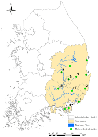
Figure 1 Locations of 12 selected weather stations in the Yeongnam province. See Table 1 for further information about the stations.

Figure 1 illustrates the locations of the selected weather stations. All the stations are inside Yeongnam province, which consists of two different regions (north and south Gyeongsang), as well as the self-governing cities of Busan, Daegu, and Ulsan. Most of the Yeongnam region is drained to the Nakdong River. To validate the proposed model appropriately, test sites must be highly correlated with each other as well as have significant temporal relation. The stations inside the Yeongnam area cover one of the most important watersheds, the Nakdong River basin, where the Nakdong River passes through the entire basin, and its hydrological assessments for agriculture and climate change have a particular value in flood control and water resources management such as floods and droughts.

Table 1 Information on 12 selected stations from the Yeongnam province, South Korea.

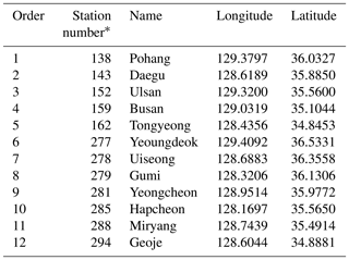
^∗ The station number indicates the identification number operated by Korea Meteorological Administration (KMA).

It is important to analyze the impact of weather conditions for planning agricultural operations and water resources management, especially during the summer season, because around 50 %–60 % of the annual precipitation occurs during the summer season from June to September. The length of daily precipitation data record ranges from 1976 to 2015 and the summer season record was employed, since a large number of rainy days occur during summer and it is important to preserve these characteristics. Also, the whole-year dataset was tested and other seasons were further applied but the correlation coefficient was relatively high and its estimated correlation matrix was not a positive semi-definite matrix for the MONR model.

5 Application

To analyze the performance of the proposed DKNNR model, the occurrence of precipitation was simulated. The DKNNR simulation was compared with that of the MONR model. For each model, 100 series of daily occurrence with the same record length were simulated. The key statistics of observed data and each generated series, such as transition probabilities (P₁₁, P₀₁, and P₁) and cross-correlation (see Eq. 10), were determined. The MONR model underestimated the lag-1 cross-correlation, as indicated by Wilks (1998). In the current study, this statistic was analyzed, since a synoptic-scale weather system often results in lagged cross-correlation for daily precipitation data (Wilks, 1998). It was formulated as

$$\begin{array}{}\text{(17)}& {\mathit{\rho }}_{\mathrm{1}}(q,s)=\mathrm{corr}[X_{t-\mathrm{1}}^q,X_t^s].\end{array}$$

Statistics from 100 generated series were evaluated by the root mean square error (RMSE), expressed as

$$\begin{array}{}\text{(18)}& \mathrm{RMSE}={\left({\displaystyle \frac{\mathrm{1}}{N}}\sum _{m=\mathrm{1}}^N{\left({\mathrm{\Gamma }}_m^G-{\mathrm{\Gamma }}^h\right)}^{\mathrm{2}}\right)}^{\mathrm{1}/\mathrm{2}},\end{array}$$

where N is the number of series (here 100), ${\mathrm{\Gamma }}_m^G$ is the statistic estimated from the mth generated series, while Γ^h is the statistic for the observed data. Note that lower RMSE indicates better performance, represented by the summarized error of a given statistic of generated series from the statistic of the observed data.

The 100 simulated statistic values were illustrated with box plots to show their variability as shown in Figs. 5–7. The box of the box plot represents the interquartile range (IQR), ranging from the 25th percentile to the 75th percentile. The whiskers extend up and down to 1.5 times the IQR. The data beyond the whiskers (1.5×IQR) are indicated by a plus sign (+). The horizontal line inside the box represents the median of the data. The statistics of the observed data are denoted by a cross (×). The closer a cross is to the horizontal line inside the box, the better the simulated data from a model reproduce the statistical characteristics of the observed data.

6 Results

6.1 GA mixing and its probability selection

The roles of crossover probability P_cr (Eq. 13) and mutation probability P_m (Eq. 14) were studied by Lee et al. (2010). In the current study, we further tested these by selecting an appropriate parameter set of these two parameters with the simulated data from the DKNNR model and the record length of 100 000. RMSE (Eq. 18) of the three transition and limiting probabilities (P₁₁, P₀₁, and P₁) between the simulated data and the observed was used, since those probabilities are key statistics that the simulated data must match the observed data, and no parameterization of these probabilities was made for the current DKNNR model. Results are shown in Figs. 2 and 3 for P_cr and P_m, respectively. For P_cr in Fig. 2, the probability of 0.02 shows the smallest RMSE in all transition and limiting probabilities. The RMSE of P_m in Fig. 3 shows a slight fluctuation along with P_m. However, all three probabilities (P₁₁, P₀₁, and P₁) have relatively small RMSEs in P_m=0.003. Therefore, the parameter set 0.02 and 0.003 was chosen for P_cr and P_m, respectively, and employed in the current study. We also tested the simulation without the GA mixing procedure (results not shown). The results showed that no better result could be found from the simulation without GA mixing. The necessity of the GA mixing is further discussed in the following.

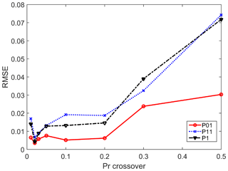
Figure 2 Testing for different probabilities of crossover P_cr. RMSE is estimated for all the tested 12 stations for each transition and limiting probability of the simulated data with the record length of 100 000.

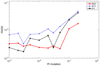
Figure 3 Testing for different probabilities of mutation P_m. RMSE is estimated for all the tested 12 stations for each transition and limiting probability of the simulated data with the record length of 100 000.

We further tested and discuss why the GA mixing is necessary in the proposed DKNNR model as follows. For example, assume that three weather stations are considered and observed data only have the occurrence cases of 000, 001, 011, 010, 011, 100, and 111, among 2³=8 possible cases. In other words, no patterns for 110 and 101 are found in the observed data. Note that 0 indicates dry days and 1 indicates rainy (or wet) days. The KNNR is a resampling process in which the simulation data are resampled from observations. Therefore, no new patterns such as 110 and 101 can be found in the simulated data.

This can be problematic for the simulation purpose in that one of the major simulation purposes is to simulate sequences that might possibly happen in the future. The wet (1) or dry (0) for multisite precipitation occurrence is decided by the spatial distribution of a precipitation weather system. A humid air mass can be distributed randomly, relying on wind velocity and direction, as well as the surrounding air pressure. In general, any combinations of wet and dry stations can be possible, especially when the simulation continues infinitely. Therefore, the patterns of simulated data must be allowed to have any possible combinations (here 4096), even if they have not been observed from the historical records. Also, the probability to have this new pattern must not be high, since it has not been observed in the historical records, and this can be taken into account by low probability of the crossover and mutation.

This drawback of the KNNR model frequently happens in multisite occurrence as the number of stations increases. Note that the number of patterns increases as 2ⁿ, where n is the number of stations. If n=12, then 4096 cases must be observed. However, among 4096 cases, observed cases are limited, since the amount of data is limited. The GA process can mix two candidate patterns to produce new patterns. For example, in the three-station case, a new pattern of 101 can be produced from two observed occurrence candidates of 001 and 100 by the crossover of the first value of 001 with the first value of 100 (i.e., 001→101), which is not in the observed data.

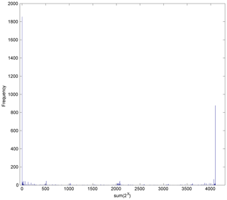
Figure 4 Frequency of the observed patterns among all the possible cases (2¹²=4096). The x coordinate indicates each pattern with the numbering of the binary number system. All zero (0) and all one (4095) have the largest and second largest numbers of frequency as 1894 and 877, respectively, as expected meaning all dry and all wet stations. Note that the bars are very sporadic, indicating a number of occurrence patterns are not observed.

Note that the data employed in the case study are 40 years and 122 days (summer months) in each year. The total number of the observed data is 4880 and the number of possible cases is 4096. We checked the number of possible cases that were not found in the observed data. The result shows that 3379 cases were not observed at all for the entire cases as shown in Fig. 4.

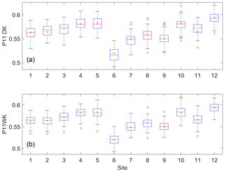
Figure 5 Box plots of the P₁₁ probability for the simulated data from the DKNNR model (a) and the MONR model (b), as well as the observed (x marker) for the 12 selected weather stations from the Yeongnam province.

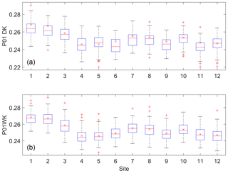
Figure 6 Box plots of the P₀₁ probability for the data simulated from the DKNNR model (a) and the MONR model (b), as well as the observed (x marker) for the 12 selected weather stations from the Yeongnam province.

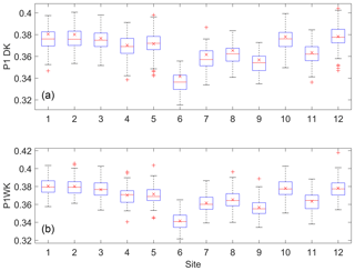
Figure 7 Box plots of the P₁ probability for the data simulated from the DKNNR model (a) and the MONR model (b), as well as the observed (x marker) for the 12 selected weather stations from the Yeongnam province.

We further investigated the number of new patterns that were generated with the probabilities P_cr=0.02, P_m=0.001 by the proposed GA mixing. The generated data for 100 sequences from DKNNR with the GA mixing show that the number 3379 was reduced to 1200, which is not in the dataset among the 4096 possible patterns. Therefore, more than 2000 new patterns were simulated with the GA mixing process. The KNNR model without the GA mixing did not produce any new patterns in the 100 sequences with the same length of the historical data.

6.2 Occurrence and transition probabilities

The data simulated from the proposed DKNNR model and the existing MONR model were analyzed. The estimated transition probabilities (P₁₁ and P₀₁ in Eq. 3) as well as the occurrence probability (P₁ in Eq. 5) are shown in Table 2 and Figs. 5–7 for the observed data and the data generated from the DKNNR and MONR models. In Table 2, the observed statistic shows that P₁₁ is always higher than P₀₁, and P₁ is between P₁₁ and P₀₁. Site 6 shows the lowest P₁₁ and P₁, and site 12 shows the highest P₁₁.

Table 2 Occurrence and transition probabilities of observed data and data simulated by DKNNR and MONR for 12 stations from the Yeongnam province, South Korea, during the summer season. Note that 100 sets with the same record length as the observed data were simulated and the statistics of 100 sets were averaged.

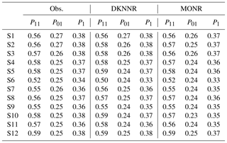
As shown in Fig. 5, the probability P₁₁ of the observed data shows that sites 6, 7, 8, and 9 located in the northern part of the region exhibited lower consistency (i.e., consecutive rainy days) than did the other sites, while sites 5 and 12 had higher probability of P₁₁ than did other sites. Both models preserved well the observed P₁₁ statistic. It seems that the MONR model had a slightly better performance, since this statistic is parameterized in the model, as shown in Sect. 2.2, and that is the same for P₀₁ and P₁, as shown in Figs. 6 and 7. Note that the MONR model employed the transition probabilities in simulating rainfall occurrence, while the DKNNR model did not. The occurrence probability P₁ can be described with the combination of transition probabilities as in Eq. (5). Even though the transition probabilities were not employed in simulating rainfall occurrence, the DKNNR model preserved this statistic fairly well.

In the DKNNR modeling procedure, the simple distance measurement in Eq. (11) allows to preserve transition probabilities in that the following multisite occurrence is resampled from the historical data whose previous states of multisite occurrence ($x_i^s$) are similar to the current simulation multisite occurrence ($X_c^s$). This summarized distance (D_i) is an essential tool in the proposed DKNNR modeling. The condition of the current weather system is memorized and the system is conditioned on simulating the following multisite occurrence with the distance measurement like a precipitation weather system dynamically changes, but often it impacts the system of the following day.

As shown in Fig. 6, the P₀₁ probability showed a slightly different behavior such that sites 1, 2, and 3 located in the middle part of the Yeongnam province showed a higher probability than did other sites. A slight underestimation was seen for sites 2 and 11 but it was not critical, since its observed value with a cross mark was close to the upper IQR representing the 75th percentile.

The behavior of P₁ was found to be the same as that of the P₁₁ probability. It can be seen in Fig. 7a that no significant underestimation is seen for the DKNNR model. The P₁ statistic was fairly preserved by both DKNNR and MONR models. Note that the MONR model parameterized the P₁ statistic through the transition probabilities as in Eq. (5), while the DKNNR model did not. Although the DKNNR model used almost no parameters for simulation, the P₁ statistic was preserved fairly well.

6.3 Cross-correlation

Cross-correlation is a measure of the relationship between sites. The preservation of cross-correlation is important for the simulation of precipitation occurrence and is required in the regional analysis for water resources management or agricultural applications. Furthermore, lagged cross-correlation is also as essential as cross-correlation (i.e., contemporaneous correlation). For example, the amount of streamflow for a watershed from a certain precipitation event is highly related to lagged cross-correlation.

Table 3 Cross-correlation of observed data for 12 stations from the Yeongnam province, South Korea.

Table 4 Averaged cross-correlation of the 100 simulated series from the DKNNR model for 12 stations from the Yeongnam province, South Korea.

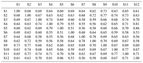
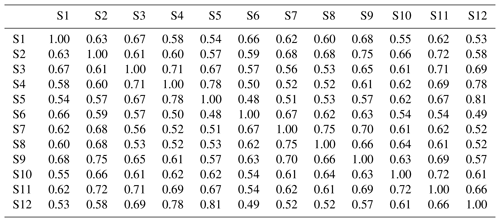
Table 5 Averaged cross-correlation of 100 simulated series from the MONR model for 12 stations from the Yeongnam province.

Daily precipitation occurrence, in general, shows the strongest serial correlation at lag-1 and its correlation decays as the lag gets longer. This is because a precipitation weather system moves according to the surrounding pressure and wind direction that dynamically change within a day or week. Therefore, we analyzed the lag-1 cross-correlation in the current study as the representative lagged correlation structure.

Table 6 The difference of RMSE of cross-correlation between MONR and DKNNR. Note that the positive value indicates that the DKNNR model performs better in preserving the cross-correlation, while a negative value (in bold font) shows that the MONR model performs better.

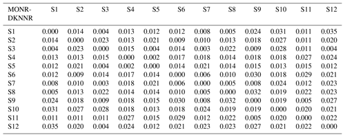
Note that no negative value can be found, implying that the DKNNR model preserves the cross-correlation better than the MONR model.

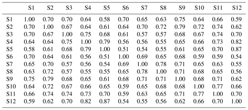
Table 7 Lag-1 cross-correlation of observed data for 12 stations from the Yeongnam province, South Korea.

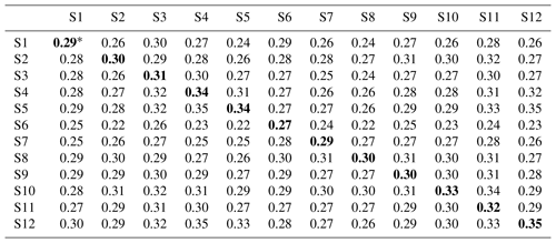
^∗ Values in bold font represent lag-1 autocorrelation (i.e., the one lagged correlation for the same site).

The cross-correlation of observed data is shown in Table 3. High cross-correlation among grouped sites, such as sites 6, 7, and 8 (northern part) and sites 3, 4, and 5, as well as 12 (southeast coastal area, 0.68–0.87), was found. As expected, sites 5 and 12 had the highest cross-correlation (0.87) due to proximity. The northern sites and coastal sites showed low cross-correlation. This observed cross-correlation was well preserved in the data generated from both DKNNR and MONR models, as shown in Fig. 8 as well as Tables 4 and 5. However, consistently slight but significant underestimation of cross-correlation was seen for the data generated by the MONR model (see Fig. 8b). Note that the error bars are extended to upper and lower lines of the circles to 1.95 times the standard deviation. The difference of RMSE in Table 6 showed this characteristic, as most of the values were positive, indicating that the proposed DKNNR model performed better for cross-correlation.

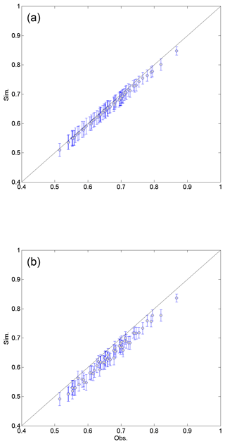
Figure 8 Scatterplot of cross-correlations between 12 weather stations for the observed data (x coordinate) and the generated data (y coordinate) from the DKNNR model (a) and the MONR model (b). The cross-correlations from 100 generated series are averaged for the filled circle, and the error bars upper and lower extended lines indicate the range of 1.95 times the standard deviation.

The lag-1 cross-correlation of observed data, as shown in Table 7, ranged from 0.22 to 0.35. The lag-1 cross-correlation for the same site (i.e., ρ₁(q,s), q=s) was autocorrelation and was highly related to P₀₁ and P₁₁ as in Eq. (6). All the lag-1 cross-correlations exhibited similar magnitudes even for autocorrelation. This implies that the lag-1 cross-correlation among the selected sites was as strong as the autocorrelation and as much as the transition probabilities P₀₁ and P₁₁ thereof.

Table 8 The difference of RMSE of lag-1 cross-correlation between MONR and DKNNR. Note that a positive value indicates that the DKNNR model performs better in preserving lag-1 cross-correlation, while a negative value (in bold font) shows that the MONR model performs better.

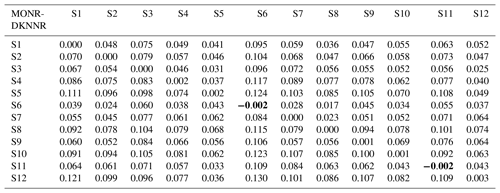
Table 9 Bias of lag-1 cross-correlation of the generated data from the DKNNR model. Note that a positive value indicates the overestimation of lag-1 cross-correlation, while a negative value shows underestimation. Note that $\mathrm{bias}=\mathrm{1}/N\sum _{m=\mathrm{1}}^N{\mathrm{\Gamma }}_m^G-{\mathrm{\Gamma }}^h$, and see Eq. (18) for the details of each term.

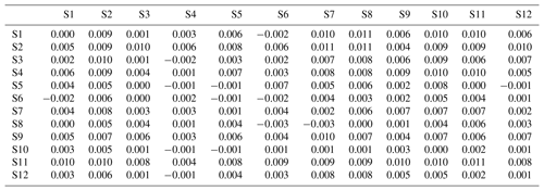
Table 10 Bias of lag-1 cross-correlation of the generated data from the Wilks model. Note that a positive value indicates the overestimation of lag-1 cross-correlation, while a negative value shows underestimation.

The observed lag-1 cross-correlations were well preserved in the data generated by the DKNNR model, as shown in Fig. 9a, while the MONR model showed significant underestimation, as seen in Fig. 9b. The difference of RMSE shown in Table 8 reflects this behavior. In Fig. 9b, some of the lag-1 cross-correlations were well preserved, that were aligned with the baseline. From Table 8, the MONR model reproduced the autocorrelations well with the shaded values. It is because the lag-1 autocorrelation was indirectly parameterized with the transition probabilities of P₁₁ and P₀₁ as in Eq. (6). Other than this autocorrelation, the lag-1 cross-correlation was not reproduced well with the MONR model. This shortcoming was mentioned by Wilks (1998). Meanwhile, the proposed DKNNR model preserved this statistic without any parameterization.

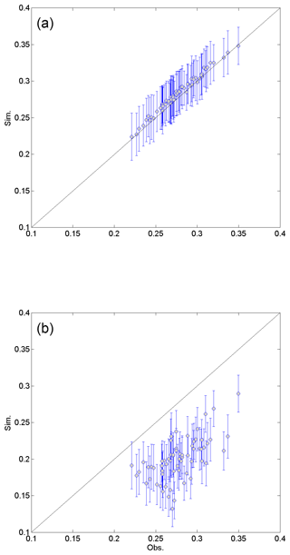
Figure 9 Scatterplot of lag-1 cross-correlations between 12 weather stations for the observed data (x coordinate) and the generated data (y coordinate) from the DKNNR model (a) and the MONR model (b). The cross-correlations from 100 generated series are averaged for the filled circle, and the error bars upper and lower extended lines indicate the range of 1.95 times the standard deviation.

We further tested the performance measurements of mean absolute error (MAE) and bias whose estimates showed that MAE had no difference from RMSE. In addition, bias of lag-1 correlation presented significant negative values, implying its underestimation for the simulated data of the MONR model as shown in Table 9, while Table 10 of the DKNNR model showed a much smaller bias.

Also, the whole-year data instead of the summer season data were tested for model fitting. Note that all the results presented above were for the summer season data (June–September), as mentioned in Sect. 4 in the data description. The lag-1 cross-correlation is shown in Fig. 10, which indicates that the same characteristic was observed as for the summer season, such that the proposed DKNNR model preserved better the lagged cross-correlation than did the existing MONR model. Other statistics, such as correlation matrix and transition probabilities, exhibited the same results (not shown). Also, other seasons were tried but the estimated correlation matrix was not a positive semi-definite matrix and its inverse cannot be made for multivariate normal distribution in the MONR model. It was because the selected stations were close to each other (around 50–100 km) and produced high cross-correlation, especially in the occurrence during dry seasons. Special remedy for the existing MONR model should be applied, such as decreasing cross-correlation by force, but further remedy was not applied in the current study since it was not within the current scope and focus.

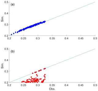
Figure 10 Scatterplot of lag-1 cross-correlations between 12 weather stations for the observed data (x coordinate) and the generated data (y coordinate) from the DKNNR model (a) and the MONR model (b) with the whole-year data and not with the summer season. The cross-correlations from 100 generated series are averaged.

6.4 Adaptation to climate change

Model adaptability to climate change in hydro-meteorological simulation models is a critical factor, since one of the major applications of the models is to assess the impact of climate change. Therefore, we tested the capability of the proposed model in the current study by adjusting the probabilities of crossover and mutation as in Eqs. (15) and (16). A number of variations can be made with different conditions.

In Fig. 11, the changes of transition and marginal probabilities are shown, along with the increase of crossover probability P_cr from 0.01 to 0.2 with the condition that the candidate value is 1 and the previous value is also 1 as in Eq. (15) for the selected 5 stations among the 12 stations (from station 1 to station 5; see Table 1 for details). The stations were limited in this analysis due to computational time. In each case, 100 series were simulated. The average value of the simulated statistics is presented in the figure. It is obvious that the transition probability P₁₁ increased as intended along with the increase of P_cr. As expected from Eq. (5), P₁ presents that the change of P₁ is highly related to P₁₁. However, the probability P₀₁ fluctuated along with the increase of P_cr. Elaborate work to adjust all the probabilities is however required.

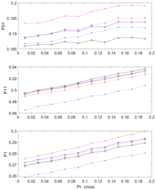
Figure 11 Transition probabilities and marginal distribution for the selected five stations along with changing the crossover probability P_cr with the condition that the candidate value is 1 and the previous value is also 1. See Eq. (15) for details.

The changes in transition and marginal probabilities are presented in Fig. 12 with increasing mutation probability P_m from 0.01 to 0.2 under the condition that the candidate value is 1, so that the marginal probability P₁ increased. P₀₁ also increased along with increasing P₁. The change of P₁₁ was not related to other probabilities. The combination of the adjustment of P_cr and P_m with a certain condition to the previous state will allow the specific adaptation for simulating future climatic scenarios.

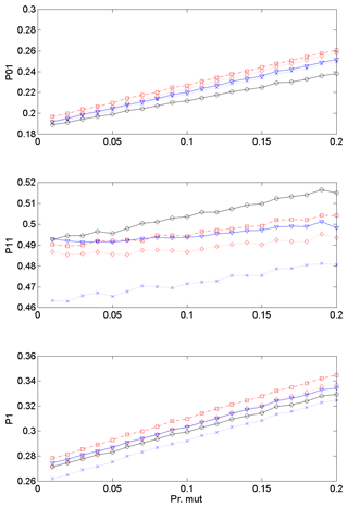
Figure 12 Transition probabilities and marginal distribution along with changing the crossover probability with the condition that the mutation is processed only if the candidate value is 1. See Eq. (16) for details.

As an example, assume that the occurrence probability (P₁) of the control period is 0.26 (see the dotted line with a cross in the bottom panels of Figs. 11 and 12) and global circulation model (GCM) output indicates that the occurrence probability (P₁) increases up to 0.27. This can be achieved with increasing either the crossover probability to 0.1 or the mutation probability to 0.05. Note that the crossover probabilities might cause the stations to affect each other, while the mutation probabilities do not.

Climate change, however, may refer to a larger phenomenon, which cannot be addressed directly through modifying only the marginal and transition probabilities as in the current study. Further model development on systematically varying temporal and spatial cross-correlations is required to properly address climate change of the regional precipitation system.

7 Conclusions

In the current study, the discrete version of a nonparametric simulation model, based on KNNR, is proposed to overcome the shortcomings of the existing MONR model, such as long stochastic simulation for parameter estimation and underestimation of the lagged cross-correlation between sites, as well as testing the adaptability for climatic change. Occurrence and transition probabilities and cross-correlation, as well as lag-1 cross-correlation are estimated for both models. Better preservation of cross-correlation and lag-1 cross-correlation with the DKNNR model than the MONR model is observed. For some cases (i.e., the whole-year data and seasons other than the summer season), the estimated cross-correlation matrix is not a positive semi-definite matrix, so the multivariate normal simulation is not applicable for the MONR model, because the tested sites are close to each other with high cross-correlation.

Results of this study indicate that the proposed DKNNR model reproduces the occurrence and transition probabilities satisfactorily and preserves the cross-correlations better than the existing MONR model. Furthermore, not much effort is required to estimate the parameters in the DKNNR model, while the MONR model requires a long stochastic simulation just to estimate each parameter. Thus, the proposed DKNNR model can be a good alternative for simulating multisite precipitation occurrence.

We further tested the enhancement of the proposed model for adapting to climate change by modifying the mutation and crossover probabilities (P_m and P_cr). Results show that the proposed DKNNR model has the capability to adapt to the climate change scenarios, but further elaborate work is required to find the best probability estimation for climate change. Also, only the marginal and transition probabilities cannot address the climate change of regional precipitation. The variation of temporal and spatial cross-correlation structure must be considered to properly address the climate change of the regional precipitation system. Further study on improving the model adaptability to climate change will follow in the near future. Also, the simulated multisite occurrence can be coupled with a multisite amount model to produce precipitation events, including zero values. Further development can be made for multisite amount models with a nonparametric technique, such as KNNR and bootstrapping.