Modular System for Shelves and Coasts (MOSSCO v1.0) – a flexible and multi-component framework for coupled coastal ocean ecosystem modelling

Shelf and coastal sea processes extend from the atmosphere through the water column and into the seabed. These processes reflect intimate interactions between physical, chemical, and biological states on multiple scales. As a consequence, coastal system modelling requires a high and flexible degree of process and domain integration; this has so far hardly been achieved by current model systems. The lack of modularity and flexibility in integrated models hinders the exchange of data and model components and has historically imposed the supremacy of specific physical driver models. We present the Modular System for Shelves and Coasts (MOSSCO; http://www.mossco.de), a novel domain and process coupling system tailored but not limited to the coupling challenges of and applications in the coastal ocean. MOSSCO builds on the Earth System Modeling Framework (ESMF) and on the Framework for Aquatic Biogeochemical Models (FABM). It goes beyond existing technologies by creating a unique level of modularity in both domain and process coupling, including a clear separation of component and basic model interfaces, flexible scheduling of several tens of models, and facilitation of iterative development at the lab and the station and on the coastal ocean scale. MOSSCO is rich in metadata and its concepts are also applicable outside the coastal domain. For coastal modelling, it contains dozens of example coupling configurations and tested set-ups for coupled applications. Thus, MOSSCO addresses the technology needs of a growing marine coastal Earth system community that encompasses very different disciplines, numerical tools, and research questions.

1 Introduction

Environmental science and management consider ecosystems as their primary subject, i.e. those systems in which the organismic world is fundamentally linked to the physical system surrounding it; there are neither unequivocally defined spatial nor processual boundaries between the components of an ecosystem (Tansley, 1935). Consequently, holistic approaches to ecological research (Margalef, 1963), biogeochemistry (Vernadsky, 1998, originally 1926), and environmental science in general (Lovelock and Margulis, 1974) have been called for.

The need for systems approaches is perhaps most apparent in coastal research. Shelf and coastal seas are described by components from different spatial domains, such as the atmosphere, ocean, soil, and they are driven by manifold interlinked processes: biological, ecological, physical, and geomorphological, amongst others. Crossing these domain and process boundaries, the dynamics of suspended sediment particles (SPM; see Appendix Appendix A for abbreviations), living particles, and the interaction between water attenuation and phytoplankton growth, for example, are both scientifically challenging and relevant for the ecological state of the coastal system (e.g.  Shang et al., 2014; Maerz et al., 2011; Azhikodan and Yokoyama, 2016).

For historical and practical reasons, the representation of the coastal ecosystem in numerical models has been far from holistic. Most often, ecological and biogeochemical processes are described in modules that are tightly coupled to one or a few hydrodynamic models. For example, the Pelagic Interactions Scheme for Carbon and Ecosystem Studies (PISCES; Aumont et al., 2015) has been integrated into the Nucleus for European Modelling of the Ocean (NEMO; Van Pham et al., 2014) and the Regional Ocean Modeling System (ROMS; Jaffrés, 2011). The Biogeochemical Flux Model (BFM) has been integrated into the Massachusetts Institute of Technology Global Circulation Model (MITgcm) (Cossarini et al., 2017) and ROMS. These tight couplings not only exclude important processes at the edges of or beyond the pelagic domain, but they also lack flexibility to exchange or to test different process descriptions.

To stimulate the development, application, and interaction of ecological and biogeochemical models independently of a single-host hydrodynamic model, Bruggeman and Bolding (2014) presented the Framework for Aquatic Biogeochemical Models (FABM), which serves as an intermediate layer between the biogeochemical zero-dimensional process models and the three-dimensional geophysical environment models. FABM has been implemented in the Modular Ocean Model (MOM; Bruggeman and Bolding, 2014), NEMO, the Finite-Volume Coastal Ocean Model (FVCOM; Cazenave et al., 2016), and the General Estuarine Transport Model (GETM; Kerimoglu et al., 2017). With more than 20 biogeochemical and ecological models included, FABM has enabled marine ecosystem researchers to describe the system's many aquatic processes.

The process-oriented modularity realised within FABM, however, lacks the means to describe cross-domain linkages. Historically rooted in atmosphere–ocean circulation models (Manabe, 1969), the coupling of Earth domains is the standard concept in Earth system models (ESMs). Domain coupling is also a major challenge in coastal modelling and has been used, for example, in the Coupled Ocean–Atmosphere–Wave–Sediment Transport (COAWST; Warner et al., 2010) system. COAWST is comprised of the Regional Ocean Modeling System (ROMS) with a tightly coupled sediment transport model, the Advanced Research Weather Research and Forecasting (WRF) atmospheric model, and the Simulating Waves Nearshore (SWAN) wave model. Each of the components in domain coupling is usually a self-sufficient model that is run in a special “coupled mode”. Interfacing to other components is done via coupling infrastructure, such as the Flexible Modeling System (FMS; Dunne et al., 2012), the Model Coupling Toolkit (MCT; Warner et al., 2008) and/or the Ocean Atmosphere Sea Ice Soil (OASIS) coupler (Craig et al., 2017), or the Earth System Modeling Framework (ESMF; Theurich et al., 2016; see Jagers, 2010 for an example intercomparison of coupling technologies). Recently, Pelupessy et al. (2017) introduced the Oceanographic Multipurpose Software Environment (OMUSE) and demonstrated nested ocean and ocean–wave domain couplings. Their intention is to provide a high-level user interface and infrastructure for coupling existing and new oceanographic models whose spatial representations differ greatly, in particular between Lagrangian- and Eulerian-type representations. The Community Surface Dynamics Modeling System (CSDMS; Peckham et al., 2013) even allows for the coupling of models implemented in many different languages, as long as all of these describe their capabilities in basic model interface (BMI; Peckham et al., 2013) descriptions. Typically, however, only three to five domain components are coupled through one of the above technologies (Alexander and Easterbrook, 2015).

The differentiation between domain and process coupling is not a technical necessity: a typical domain coupling software like ESMF can also be used to couple processes. With the Modeling Analysis and Prediction Layer (MAPL; Suarez et al., 2007), the Goddard Earth Observing System version 5 (GEOS-5) encompasses 39 process models coupled hierarchically through ESMF. The development of these modules, however, is strictly regulated within the developing laboratory. Vice versa, a typical process coupling infrastructure like the Modular Earth Submodel System (MESSy; Jöckel et al., 2005), which initially linked mostly atmospheric processes, has been generalised to support linking at a user-chosen granularity regardless of the process versus domain dichotomy (e.g. Kerkweg and Jöckel, 2012).

Up to now, there has been no coastal modelling environment that enables a modular and flexible process (model) integration and cross-domain coupling at the same time that is open to a larger community of independent biogeochemical and ecological scientists. The underlying long-term goal for increasingly holistic model systems conflicts with the evolving and diverse research needs of individual scientists or research groups to address very specific problems; it remains difficult to link up-to-date research that is delivered on the (local) process scale to the Earth system scale. Thus we present the Modular System for Shelves and Coasts (MOSSCO, http://www.mossco.de), a novel system for domain and process coupling that is tailored but not limited to the coupling challenges of and applications in the coastal ocean. This new system builds on the flexibility of FABM and on the infrastructure provided by ESMF with its cross-domain and many-component hierarchical capability. We present the major design ideas of MOSSCO and briefly demonstrate its usability in a series of coastal applications.

2 MOSSCO concepts

The modularity and coupling concepts proposed in this paper describe a novel software system that addresses the needs of researchers who want to make maximum use of their existing knowledge in a specific field (e.g. geomorphology or marine ecology) but wish to conduct integrative research in a wider and flexible context. In strengthening the independence from specific physical drivers, the new concept should, in addition to addressing the problems listed above, support (1) liaisons between traditionally separated modelling communities (e.g. coastal engineers, physical oceanographers, and biologists), (2) intercomparison studies of physical, geological, and biological modules, and (3) up-scaling studies in which models developed on the laboratory scale in a non-dimensional context are applied to regional, global, and Earth system scales.

The design of MOSSCO is application oriented and driven by the demands for enabling and improving integrated regional coastal modelling. It is targeted towards building coupled systems that support decision making for local policies implementing the European Union Water Framework Directive (WFD) and Marine Strategic Planning Directive (MSPD). From a design point of view we envisioned a system that is foremost flexible and equitable.

Flexibility

means that the system itself is able to deal on the one hand with a diverse small or large constellation of coupled model components and on the other hand with different orders of magnitude of spatial and temporal resolutions; it is able to deal equally well with zero-, one-, two-, and three-dimensional representations of the coastal system. Flexibility implies the capability to also encapsulate existing legacy models to create one or more different “ecosystems” of models. This feature should allow for the seamless replacement of individual model components, which is an important procedure in the continual development of integrated systems. Flexibly in replacing components finally creates a test bed for model intercomparison studies.

Equitability

means that all models in the coupled framework are treated as equally important and that none is more important than any other. This principle dissolves the primacy of the hydrodynamic or atmospheric models as the central hub in a coupled system. Also, data components are as important as process components or model output; any de facto difference in model importance should be grounded in the research question and not on technological legacy. As complexity grows by coupling more and more models, this equitability also demands that experts in one particular model can rely on the functionality of other components in the system without having to be an expert in those models as well.

Flexibility

means that the system itself is able to deal on the one hand with a diverse small or large constellation of coupled model components and on the other hand with different orders of magnitude of spatial and temporal resolutions; it is able to deal equally well with zero-, one-, two-, and three-dimensional representations of the coastal system. Flexibility implies the capability to also encapsulate existing legacy models to create one or more different “ecosystems” of models. This feature should allow for the seamless replacement of individual model components, which is an important procedure in the continual development of integrated systems. Flexibly in replacing components finally creates a test bed for model intercomparison studies.

Equitability

means that all models in the coupled framework are treated as equally important and that none is more important than any other. This principle dissolves the primacy of the hydrodynamic or atmospheric models as the central hub in a coupled system. Also, data components are as important as process components or model output; any de facto difference in model importance should be grounded in the research question and not on technological legacy. As complexity grows by coupling more and more models, this equitability also demands that experts in one particular model can rely on the functionality of other components in the system without having to be an expert in those models as well.

The equitability design extends to participation: contributions to the development of components or the coupling framework itself is allowed and encouraged. Anyone can use and modify the coupled framework or parts of both in a legal sense through open source licencing and in an accessibility sense through template codes and extensive documentation.

2.1 Wrapping legacy models – first steps in PARSE

Figure 1 MOSSCO's adoption of legacy code follows the two-layer paradigm of BMI–CMI (basic model interface–component model interface) suggested by Peckham et al. (2013). An existing legacy code (illustrated by “some model”) is enhanced by model-specific code that exhibits basic coupling functionality (BMI) and is framework agnostic. In a second step, a component (CMI) is added that uses the BMI in the specific application programming interface of the coupling framework. In addition to model interfaces that can be used in MOSSCO-independent contexts, MOSSCO provides coupling concepts and working implementations for coupled applications.

As MOSSCO is built around the ESMF hierarchy of components, any existing code that can be wrapped in an ESMF component can be a component in MOSSCO, too. The ESMF user guide (ESMF Joint Specification Team, 2013) suggests a best practice method, PARSE, to achieve this componentisation of a legacy code.

P

repare the user code by splitting it into three phases that initialise, run, and finalise a model.

A

dapt the model data structures by wrapping them in ESMF infrastructure like states and fields.

R

egister the user's initialise, run, and finalise routines through ESMF.

S

chedule data exchange between components.

E

xecute a user application by calling it from an ESMF driver.

This PARSE concept allows for a smooth transition from a legacy model to an ESMF component. In this concept, the first three steps have to be performed on the model side and the latter two on the framework side and have been taken care of by the MOSSCO coupling layer. The preparation of the code is independent of the use of ESMF and provides the basic coupling ability – or “coupleability” – of the model; many existing models already implement this separation into initialise, run, and finalise phases, either structurally or more formally by implementing a BMI. For the run phase, it is mandatory to refer to a single model timestep and not to the entire run loop.

The adaption of a model's internal structures to ESMF consists of technically wrapping data into ESMF communication objects and providing sufficient metadata for communication. Among these are the grid definition and decomposition, units, and semantics of data, optimally following a metadata scheme like the widespread Climate and Forecast (CF; Eaton et al., 2011) or the more bottom-up Community Surface Dynamics Modeling System (CSDMS; following a scheme like object + operation + quantity; Peckham, 2014). Both are currently being included in the emerging Geoscience Standard Names Ontology (GSN; http://geoscienceontology.org).

ESMF provides the interfaces for models written in either the Fortran or C programming languages; data arrays are bundled together with related metadata in ESMF field objects. All field objects from components are then bundled into exported and imported ESMF state objects to be passed between components. As a third step, the ESMF registration facility, needs to be added to a user model; this step is achieved by using template code from any one of the examples or tutorials provided with ESMF. The second and third step (adapt and register) are typical tasks of what Peckham et al. (2013) refer to as a component model interface (CMI); it is very similar between models (and thus easily accessible from template code) and targets the interface of a specific coupling framework.

MOSSCO contains CMIs for ESMF in all of its provided components (Fig. 1). The current naming scheme follows the CF convention for standard names except for quantities that are not defined by CF; these names (often from biological processes) are modelled onto existing CF standard names as much as possible. MOSSCO also allows for specification within other naming schemes and includes a name-matching algorithm to mediate between different schemes. For future development, adoption of the GSN ontology is foreseen.

2.2 Scheduling in a coupled system – the “S” in PARSE

Figure 2 Scheduling of three coupled component instances A, B, C and their data exchanges according to a pairwise coupling specification (see Fig. 3b); shown along a simulation time axis, which is independent of the type of (sequential or concurrent) deployment. Note how each individual component instance has varying run lengths resulting from the interference of all coupling intervals with this component. The time steps of the (anonymous) scheduler component t_k+n (grey bars) vary according to the interference pattern of all coupling intervals. Coupling specification (Fig. 3): A couples bidirectionally to B at interval Δt_AB (green), A couples unidirectionally to C via a coupler D at interval Δt_AC (blue), C couples unidirectionally to B at interval Δt_CB (black).

MOSSCO adds onto ESMF a scheduling system (corresponding to the fourth step in PARSE) that calls the different phases of participating coupled models. The coupling time step duration of this new scheduler relies on the ESMF concept of alarms and a user specification of pairwise coupling intervals between models. The scheduler minimises calls to participating models by flexibly adjusting time step duration to the greatest common denominator of coupling intervals pertinent to each coupled model. Upon reading the user's coupling specification, (i) models are initialised in random order but with consideration of special initialisation dependencies set by the user; (ii) a list of alarm clocks is generated that considers all pairwise couplings a model is involved in; (iii) special couplers associated with a pairwise coupling are executed; (iv) the scheduler then tells each model to run until that model reaches its next alarm time; and (v) the advancing of the scheduler to the minimum next alarm time repeats until the end of the simulation.

The MOSSCO scheduler allows for both sequential and concurrent coupling of model components or a hybrid coupling mode. In the concurrent mode, components run at the same time on different computing resources; in the sequential mode, components are executed one after another on the same set of computing resources. Recently, Balaji et al. (2016) demonstrated how a hybrid coupling mode and fine granularity could be used to increase the performance of a system that consists of both highly scalable and less scalable components. In their system, an ocean and an atmosphere component run concurrently; within the atmospheric component, the radiation code is executed concurrently to a composite component that encompasses a sequential coupling of all non-radiative atmospheric processes.

For both concurrent and sequential modes, coupling between components is explicit: the MOSSCO scheduler runs the connectors and mediator components that exchange the data before the components are run. For sequential mode, the coupling configuration also allows for a memory efficient scheme in which consecutive components operate on shared data that always reflect the most recently calculated data from the previous component (Fig. 2; see also Sect. 3.3.1); such sequential coupling on shared data potentially introduces mass imbalances.

Figure 3 Examples of coupling configurations (a, b) and the steps from installation to deployment (c). The configurations exhibit a minimal default coupling specification (a) and a more complex one (b, see Fig. 2) that makes use of dependencies, instantiation, and different coupling intervals. The line-numbered installation steps (c) include environment variable specification (export), download of the system with git, loading additional external models with make, installation of the mossco executable script, and finally deployment of the coupling specification jfs in a predefined set-up called “helgoland”, a 1-D station near the island of Helgoland in the southern North Sea.

Users specify the coupling in a text format using YAML (short for YAML Ain't Markup Language; http://yaml.org) notation, a human-reader-friendly data serialisation standard. The item coupling contains a list of components that itself contains a list of coupled components; in the simple example (Fig. 3a) two components named “A” and “B” are coupled. By default, these components are coupled in sequential mode with the default connector sharing their data; the execution order of A and B is not specified. In a more elaborate example (Fig. 3b), the order of components in the scheduler is specified in the dependency section, indicating a run sequence of first A, then B, and last C; all components run on the same set of computing resources in (default) sequential coupling mode.

The instances section declares that the component named C is an instance (or copy) of A; this makes it possible to reuse components multiple times in (possibly different) configurations. Typically, data reader or writer components are instantiated from a generic input–output component to access different files for model input and output. Multiple couplings between the three components A, B, and C are present with coupling intervals that lead to the scheduling of coupling events according to Fig. 2. Between A and C, a special coupler “D” handles the data exchange instead of the default connector.

2.3 Deployment of the coupled system – the “E” in PARSE

MOSSCO provides a Python-based generator that dynamically creates an ESMF driver component in a star topology that then acts as the scheduler for the coupled system. This generator reads the specification of pairwise couplings (Fig. 3) and generates a Fortran source file that represents the scheduler component. The generator takes care of compilation dependencies of the coupled models and of coupling dependencies, such as grid inheritance; in addition to the basic init–run–finalise BMI scheme, it also honours multi-phase initialisation (as in the National Unified Operational Prediction Capability, NUOPC, ESMF extension) and a restart phase. The generated code structurally and functionally resembles a NUOPC driver, but it does not require implementation of the NUOPC extension, which is currently restricted to handling only structured grid-based sub-models.

A MOSSCO command line utility provides a user-friendly interface to generating the scheduler, (re-)compiling all source codes into an executable and submitting the executable to a multi-processor system, including different high-performance computing (HPC) queueing implementations; this is the fifth step in PARSE. By designing this command line utility and automatic scheduler component creation based on the simple YAML textual coupling specification, MOSSCO provides a fast way to reconfigure, rearrange, extend, or reduce coupled systems very quickly in contrast to more elaborate graphical coupling tools such as the CUPID Eclipse interface (Dunlap, 2013, only for NUOPC).

MOSSCO has been successfully deployed at several national HPC centres, such as the Norddeutsche Verbund für Hoch- und Höchstleistungsrechnen (HLRN), the German Climate Computing Center (DKRZ), and the Jülich Supercomputing Centre (JSC). Equally, MOSSCO is currently functioning on a multitude of Linux and macOS laptops, desktops, and multiprocessor workstations using the same MOSSCO (bash-based) command line utility on all platforms.

The MOSSCO coupling layer is coded in Fortran, while most of the supporting structure is coded in Python and partially in bash syntax. The system requirements are a Fortran 2003 compliant compiler, the CMake build system, the Git distributed version control system, Python with YAML support (version 2.6 or greater), a Network Common Data Form (NetCDF; Rew and Davis, 1990) library, and ESMF (version 7 or greater). For parallel applications, a message-passing library (e.g. OpenMPI) is required. Many HPC centres have toolchains available that already meet all of these requirements. For an individual user installation, all requirements can be taken care of with one of the package managers distributed with the operating system, except for the installation of ESMF, which needs to be manually installed; MOSSCO provides a semi-automated tool for helping in this installation of ESMF. The steps to get MOSSCO running quickly on any suitable computer system are outlined in Fig. 3c. These instructions should get a reader started on carrying out initial simulations with a coupled system by typing a dozen lines of code, provided that all requirements are met.

3 MOSSCO components and utilities

Table 1 Components currently integrated into MOSSCO and described shortly in this paper. Several other components are under development and not listed here.

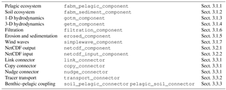
Driven by user needs, MOSSCO currently entails utilities for I/O, an extensive model library, and coupling functionalities (Fig. 4 and Table 1). As a utility layer on top of ESMF, MOSSCO also extends the application programming interface (API) of ESMF by providing convenience methods to facilitate the handling of time, metadata (attributes), configuration, and to unify the provisioning and transfer of scientific data across the coupling framework. The use of this utility layer is not mandatory; any ESMF-based component can be coupled to the MOSSCO-provided components without using this utility layer.

One of the major design principles of MOSSCO is seamless deployment from zero-dimensional to three-dimensional spatial representations, while maintaining the coupling configuration to the maximum extent possible. This design principle builds on the dimensional independency concept of FABM achieved by the local description of processes (often referred to as a box model), in which the dimensionality is defined by the hydrodynamic model to which FABM is coupled. MOSSCO generalises this concept to enable the developers of new biological and chemical models to scale up from a box model (zero-dimensional) to a water column (one-dimensional), sediment plate, or a vertically resolved transect (two-dimensional) and a full atmosphere or ocean (three-dimensional) set-up. As a concrete example, the novel Model for Adaptive Ecosystems in Coastal Seas (MAECS; Wirtz and Kerimoglu, 2016; Kerimoglu et al., 2017) has been developed, iterating between an application for the lab (zero-dimensional) scale and the three-dimensional regional coastal ocean scale.

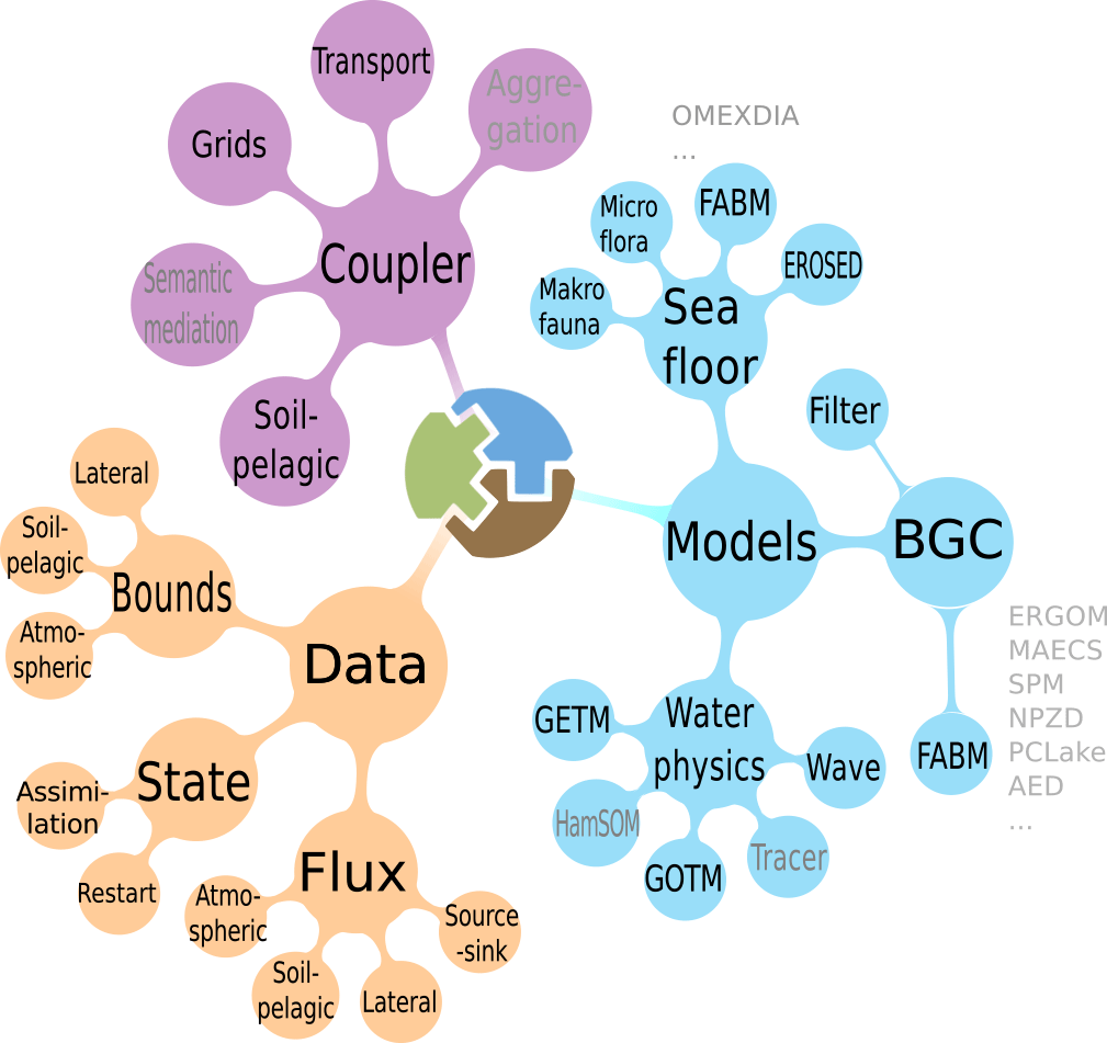
Figure 4 Modular components of MOSSCO. The blue branch collects newly created sub-models and components that wrap around legacy codes; the violet branch collects coupling functionalities and the orange branch the input–output utilities.

All utility functions and components, especially the model-independent I/O facilities from MOSSCO, are able to handle data of any spatial dimension. Components that do not define their own spatial representation as a grid or mesh are able to inherit the complete spatial information from a coupled component that provides such a grid: usually (but not necessarily) biological and chemical models inherit the spatial configuration from a hydrodynamic model. Equally, this information can be obtained from data in standardised grid description formats like Gridspec (Balaji et al., 2007) or the Spherical Coordinate Remapping and Interpolation Package (SCRIP; Jones, 1999). Grid inheritance is specified as a dependency in the coupling specification.

3.1 Model library: model interfaces for scientific model components

The model library (right branch in Fig. 4) includes new models (e.g. for filter feeders and surface waves) and wrappers to legacy models and frameworks such as FABM or GETM. Some of these wrappers are under development, among them the Hamburg Shelf Ocean Model (HamSOM; Harms, 1997) and a Lagrangian particle tracer model. Here, we briefly document the model collection, particularly with respect to their preparation and functioning within the new coupling context.

3.1.1 Pelagic ecosystem component

The pelagic ecosystem component (fabm_pelagic_component) collects (mostly biological) process models for aquatic systems. This component makes use of the Framework for Aquatic Biogeochemical Models (Bruggeman and Bolding, 2014). FABM is a coupling layer to a multitude of biogeochemical models which provide the source-minus-sink terms for variables, their vertical local movement (e.g. due to sinking or active mobility), and diagnostic data. Each model variable is equipped with metadata, which is transferred by the ecosystem component into ESMF field names and attributes. Similarly, the forcing required by the biogeochemical models is communicated within the framework and linked to FABM. The pelagic ecosystem component includes a numerical integrator for the boundary fluxes and local state variable dynamics. Advective and diffusive transport are not part of this component but are left to the hydrodynamical model through the transport_connector (Sect. 3.3.2). The close connection between transport and the pelagic ecosystem requires that the spatial representation of the FABM state variables be inherited from the hydrodynamic model component that performs the transport calculations.

Many well-known biogeochemical process models have been coded in the FABM standard by various institutes, such as the European Regional Seas Ecosystem Model (ERSEM; Butenschön et al., 2016), ERGOM (Hinners et al., 2015), PCLake (Hu et al., 2016), and the Bottom RedOx Model (BROM; Yakushev et al., 2017). All pelagic biogeochemical models complying with the FABM standard can equally be used in MOSSCO, while retaining their functionality.

3.1.2 Sediment and soil component

The sediment component fabm_sediment_component hosts (mostly biogeochemical) process descriptions for aquatic soils. To allow for efficient coupling to a pelagic ecosystem, the sediment component inherits a horizontal grid or mesh from the coupled system and adds its own vertical coordinate, a number of layers of horizontally equal height for the upper soil (typical domain heights range from 10–50 cm). State variables within the sediment are defined through the FABM framework within the 3-D grid or mesh in the sediment. As in the pelagic ecosystem component, the state variables, metadata, diagnostics, and forcings are communicated via the ESMF framework to the coupled system. The sediment component is the numerical integrator for the tracer dynamics within each sediment column in the horizontal grid or mesh, including diffusive transport, driven by molecular diffusion of the nutrients or bioturbative mixing. Additionally, a 3-D variable porosity defines the fraction of pore water as part of the bulk sediment, while all state variables are measured per volume of pore water in each cell. The FABM infrastructure of state variable properties is used to label the new boolean property particulate in FABM models to define whether a state variable belongs to the solid phase within the domain. A typical model used in applications of the sediment component is the biogeochemical model of the Ocean Margin Exchange Experiment OMEXDIA (Soetaert et al., 1996); a version of this model with added phosphorous cycle is contained in the FABM model library as OMEXDIA_P (Hofmeister et al., 2014).

3.1.3 1-D Hydrodynamics: General Ocean Turbulence Model (GOTM))

The General Ocean Turbulence Model (GOTM; Burchard et al., 1999, 2006) is a one-dimensional water column model for hydrodynamic and thermodynamic processes related to vertical mixing. MOSSCO provides a component for GOTM and a component hierarchy that considers a coupled GOTM with internally coupled FABM within one component (gotm_fabm_component), as many existing available model set-ups rely on the direct coupling of FABM to GOTM. This way, the modularisation – taking a coupled GOTM–FABM apart and recoupling it through the MOSSCO infrastructure – can be verified; the encapsulation of GOTM is implemented in the gotm_component.

3.1.4 3-D Hydrodynamics: General Estuarine Transport Model (GETM)

MOSSCO provides an interface to the 3-D coastal ocean model GETM (Burchard and Bolding, 2002). GETM solves the Navier–Stokes equations under Boussinesq approximation, optionally including the non-hydrostatic pressure contribution (Klingbeil and Burchard, 2013). A direct interface to GOTM (see Sect. 3.1.3) provides state-of-the-art turbulence closure in the vertical. GETM supports horizontally curvilinear and vertically adaptive meshes (Hofmeister et al., 2010; Gräwe et al., 2015). The interface to GETM is provided by the getm_component; any model coupled to GETM via the transport component can have its state variables conservatively transported by GETM (see Sect. 3.3.2). In the component, the GETM-created spatial topology is made available as an ESMF grid object; typically this grid and subdomain decomposition is communicated to the coupled system in which the spatial and parallelisation information is inherited by other components.

3.1.5 Model components for erosion, sedimentation, and their biological alteration

The erosion and sedimentation routines of the Deltares Delft3D model (EROSED; van Rijn, 2007) were encapsulated in a MOSSCO component. EROSED uses a Partheniades–Krone equation (Partheniades, 1965) for calculating the net sediment flux of cohesive sediment at the water–sediment interface for multiple SPM size classes. The MOSSCO BMI uses the current version of EROSED maintained by Deltares; it isolates with the help of subsidiary infrastructure the original code from the deeply intertwined dependencies in the Delft3D system. The erosed_component can provide its own spatial representation as a structured grid or unstructured mesh; it can also inherit the spatial information from a coupled component. The functionality of the erosion and sedimentation component is described in more detail by Nasermoaddeli et al. (2014).

Flow and sediment transport can be affected by the presence of benthic organisms in many ways. Protrusion of benthic animals and macrophytes in the boundary layer changes the bed roughness and thus the bed shear stress and consequently the sediment transport. The erodibility of sediment can be modified by the mucus produced by benthic organisms; the erodibility of the upper bed sediment can be altered by bioturbation generated by macrofauna (de Deckere et al., 2001). In the benthos_component, these biological effects of microphytobenthos and of benthic macrofauna on sediment erodibility and critical bed shear stress are parameterised and provided to other coupled components (e.g. the erosion and sedimentation component) as additional erodibility and critical shear stress factors. The benthos effect model is described in detail by Nasermoaddeli et al. (2018).

3.1.6 Filter feeding model

The filtration_component describes the instantaneous filtration by suspension feeders within the water column. This biological filtration model follows Bayne et al. (1993) and describes the filtration rate as a function of food supply; it can be adapted to different species of filter feeders and was recently applied to describing the ecosystem effect of blue mussels on offshore wind farms as the filtration_component of MOSSCO (Slavik et al., 2018). The filtration model uses an arbitrary chemical species or compound, for example phytoplankton carbon, as the “currency” for processing. The ambient phytoplankton carbon concentration is sensed by the model organisms and filtered along with the other nutrients (in stoichiometric proportion) out of the environment, creating a sink term for subsequent numerical integration in the pelagic ecological model.

3.1.7 Wind waves

A simple wind wave model is part of the MOSSCO suite. Based on the parameterisation by Breugem and Holthuijsen (2007), significant wave height and peak wave period are estimated in terms of local water depth, wind speed, and fetch length. This wave data enable the inclusion of wave effects, especially for idealised 1-D water column studies, e.g. the consideration of erosion processes due to wave-induced bottom stresses. Coupling to 3-D ocean models and the calculation of additional wave-induced momentum forces, following either the radiation stress or vortex force formulation (Moghimi et al., 2013), is possible as well. For the inclusion of wave–wave or wave–current interactions in realistic 3-D applications, coupling to a more advanced third-generation wind wave model like SWAN, WaveWatch III, or a wave atmospheric model (WAM) would be necessary.

3.2 Input–output utilities

The input and output (I/O) utilities include general purpose coupling functionalities that deal with boundary conditions, provide a restart facility, and add surface, lateral, and point source fluxes (lower left branch in Fig. 4).

3.2.1 NetCDF output

This component of MOSSCO provides an output facility netcdf_component for any data that are communicated in the coupling framework. The component writes one- to three-dimensional time-sliced data into a NetCDF (Rew and Davis, 1990) file and adds metadata on the simulation to this output. Multiple instances of this component can be used within a simulation such that output of different variables, differently processed data, and output at various time steps can be recorded. The output component is fully parallelised with a grid decomposition inherited from one of the coupled science or data components. In order to reduce interprocess communication during runtime, each write process considers only the part of the data (its data tile) that resides within its computing domain. This comes at a cost to the user, who has to post-process the output tiles to combine for later analysis; a Python script is provided with MOSSCO that takes care of joining tiled files.

The output component also adds metadata that is collected from the system and the user environment at the creation time of the output files. Diagnostics on the processing element and run time between output steps are recorded. The structure of the NetCDF output follows the Climate and Forecast (CF; Eaton et al., 2011) convention for physical variables, geolocation, units, dimensions, and methods modifying variables. When (mostly biological) terms are not available in the controlled vocabulary of CF, names are built to resemble those contained in the standard.

3.2.2 NetCDF input

The netcdf_input_component of MOSSCO reads from NetCDF files and provides the file content wrapped in ESMF data structures (fields) to the coupling framework. It inherits its decomposition from other components in the coupled system. Data can be read from a single file for the entire domain or from distributed files for all decomposed computing elements separately. Upon reading data, fields can be renamed and filtered before they are passed on to the coupled system.

The input component is typically used to initialise other components for restarting, to provide boundary conditions, and for assimilating data into the coupled system. The input facility supports the interpolation of data in time upon reading the data with nearest, most recent, and linear interpolation. It also supports reading climatological data and translates the climatological time stamp to a simulation present time stamp in the coupling framework.

3.3 MOSSCO connectors and mediators

Information in the form of ESMF states that contain the output fields of every component are communicated to the ESMF driver; requests for data by every component are also communicated to the ESMF driver component. MOSSCO connectors are separate components that link the output and requested fields between pairwise coupled components. MOSSCO informally distinguishes between connector components that do not manipulate the field data on transfer at all (or only slightly) and mediator components that extract and compute new data out of the input data.

3.3.1 Link, copy, and nudge connectors

The simplest and default connecting action between components is to share a reference (i.e. a link) to a single field that resides in memory and can be manipulated by each component; in contrast, the copy_connector duplicates a field at coupling time. The consideration of a link or copy connector is important for managing the data flow sequence in a coupled system: the copy mechanism ensures that two coupled components work on the same lagged state of data, whereas the link mechanism ensures that each component works on the most recent data available.

The nudge_connector is used to consolidate output from two components through the weighted averaging of the connected fields. It is typically used as a simple assimilation tool to drive model states towards observed states or to impose boundary conditions.

These connectors can only be applied between components that run on the same grid (but maybe with a different subdomain decomposition). The link_connector can only be applied between components with an identical subdomain decomposition so that the components have access to the same memory. Components on different grids require regridding, which is currently under development in MOSSCO.

3.3.2 Transport connector

A model component qualifies as a transport component when it offers to transport an arbitrary number of tracers in its numerical grid; this facility is present, for example, in the current gotm_component and getm_component. The transport_connector collects state variables to be transported from any coupled component and communicates this collection to the hydrodynamic component based on the availability of both the tracer concentrations and their rate of vertical movement independent of the water currents. This connector is usually called only once per coupled pair of components during the initialisation phase.

3.3.3 Mediators for soil–pelagic coupling

One aspect of the generalised coupling infrastructure in MOSSCO is the use of connecting components that mediate between technically or scientifically incompatible data field collections. The soil–pelagic coupling of biogeochemical model components with a variety of different state variables raises the need for these mediators. The use of mediators leaves the level of data aggregation, data disaggregation, and unit conversion to the coupling routine instead of requiring specific output from a model component depending on its coupling partner component.

For soil–pelagic (or benthic–pelagic) coupling, the soil_pelagic_connector mediates the soil biogeochemistry output towards the pelagic ecosystem input and the pelagic_soil_connector mediates the pelagic ecosystem output towards the soil biogeochemistry input. Examples include the following: (i) disaggregation of dissolved inorganic nitrogen to dissolved ammonium and dissolved nitrate; (ii) filling missing pelagic state fields for phosphate using the Redfield equivalent for dissolved inorganic nitrogen; and (iii) calculation of the vertical flux of particulate organic matter (POM) from the water column into the sediment depending on POM concentrations in the near-bottom water, its sinking velocity, and a sedimentation efficiency depending on the near-bottom turbulence. The effective vertical flux is communicated into the pelagic ecosystem component to budget the respective loss and is communicated to the soil biogeochemistry component to account for the respective new mass of POM. The mediator also handles (iv) disaggregation of a single oxygen concentration (allowing for positive and negative values) into dissolved oxygen concentration, if positive, and dissolved reduced substances, if negative, and (v) aggregation of pelagic POM composition (variable nitrogen to carbon ratio) into fixed stoichiometry POM pools in the soil biogeochemistry.

4 Selected applications as feasibility tests and use cases

MOSSCO was designed for enhancing flexibility and equitability in environmental data and model coupling. These design goals have been helpful in generating new integrated models for coastal research with applications at different marine stations (1-D), transects (2-D), and sea domains (3-D). Below, we describe from a user perspective the added value and success of the design goals obtained from using MOSSCO in selected applications; here, the focus is not on the scientific outcome of the application (these are described elsewhere by Nasermoaddeli et al., 2018, Slavik et al., 2018, and Kerimoglu et al., 2017). All set-ups described in the use cases are available as open source (with limited forcing data due to space and bandwidth constraints).

4.1 Helgoland station

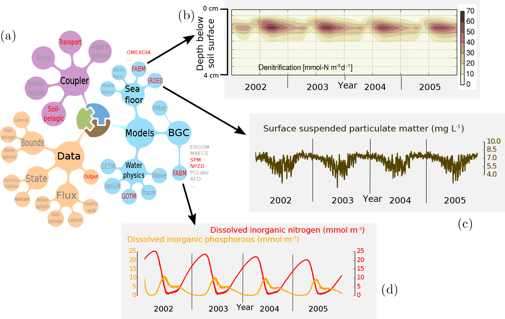
Figure 5 Coupling set-up and exemplary results from a 1-D system simulating the nutrient and SPM dynamics near the island of Helgoland, Germany with soil–pelagic coupling from 2002 to 2005. (a) Coupling set-up with seven ESMF components (highlighted in red, leaves) and three FABM sub-models (side text); (b) soil denitrification rate; (c) surface SPM dynamics resulting from EROSED and pelagic FABM–SPM; (d) middle water column nitrogen and phosphorous dynamics from pelagic FABM–NPZD.

The seasonal dynamics of nutrients and turbidity emerge from the interaction of physical, ecological, and biogeochemical processes in the water column and the underlying sea floor. We resolve these dynamics in a coupled application for a 1-D vertical water column for a station near the German offshore island of Helgoland. Average water depth around the island is 25 m; tidal currents are affected by the M2 and S2 tides with a characteristic spring–neap cycle, with current velocity not exceeding 1 m s⁻¹.

The Helgoland 1-D application is realised by a coupled system consisting of GOTM hydrodynamics, the pelagic FABM component with a nutrient–phytoplankton–zooplankton–detritus (NPZD) ecosystem model (Burchard et al., 2005), and two SPM size classes interacting with the erosion and sedimentation module, the sediment component with the OMEXDIA_P early diagenesis sub-model, and coupler components for soil–pelagic, pelagic–soil, and tracer transport. This system and set-up are described in more detail by Hofmeister et al. (2014).

Simulations with this application show a prevailing seasonal cycle in the model states (Fig. 5). Dissolved nutrients (referred to as dissolved inorganic nitrogen) are taken up by phytoplankton, which fills the pool of particulate organic nitrogen during the spring bloom (Fig. 5d). The particulate organic matter sinks into the sediments, where it is remineralised along axis, sub-oxic, and anoxic pathways; denitrification, for example, shows a peak in late summer (Fig. 5b). At the end of a year, nutrient concentrations are high in the sediment and diffuse back into the water column up to winter values of 20–25 mmol m⁻³. The seasonal variation of turbidity is a result of higher erosion in winter and reduced vertical transport in summer (Fig. 5c).

4.2 Idealised coastal 2-D transect

The coastal nitrogen cycle is resolved in an idealised coupled system for a tidal shallow sea. This two-dimensional set-up represents a vertically resolved cross-shore transect 60 km in length and at 5–20 m of water depth and has been used by Hofmeister et al. (2017) to simulate sustained horizontal nutrient gradients by particulate matter transport towards the coast. Within the MOSSCO coupling framework, the 2-D transect scenario additionally provides insights into the horizontal variability of erosion–sedimentation and benthic biogeochemistry. Its coupling configuration builds on the one used for the 1-D station Helgoland (Sect. 4.1); the water column hydrodynamic model GOTM, however, is replaced by the 3-D model GETM; a local wave component and data components for open boundaries and restart have been added.

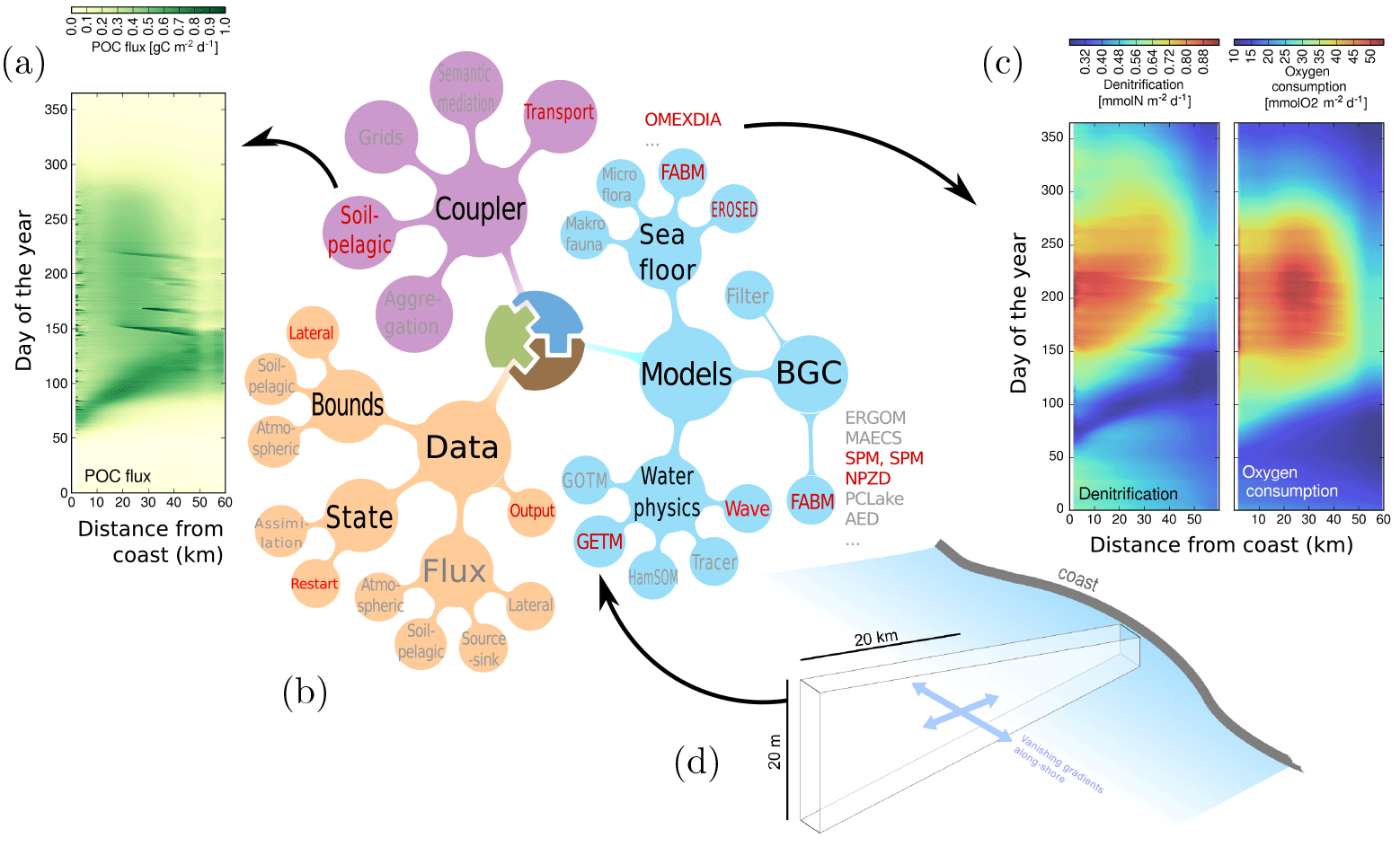
Figure 6 A 2-D idealised cross-shore transect off the German coastline is used to investigate the feedback loop among estuarine circulation, sediment transport, and nutrient cycling across the benthic–pelagic interface. (a, c) Hovmöller diagrams showing the soil–pelagic fluxes of particulate organic carbon (POC) and the soil BGC denitrification and oxygen consumption rates for the 60 km long transect. (b) Coupling diagram including components for hydrodynamics, erosion–sedimentation, waves, pelagic ecology, suspended particles, and soil ecology. This example uses both ESMF modularity (the components) and FABM modularity (the different ecological–biogeochemical models within the pelagic and sediment environmental components). (d) Spatial set-up of the idealised 2-D cross-shore transect.

Figure 6 shows exchange fluxes between the water column and the sediment for 1 year of simulation. The simulation of turbidity, as a result of pelagic SPM transport and resuspension by currents and wave stress, provides the light climate for the pelagic ecosystem. The flux of particulate organic carbon (POC) into the sediment reflects bloom events in summer during calm weather conditions. Macrobenthic activity in the sea floor brings fresh organic matter into the deeper sub-oxic layers of the sediment, where denitrification removes nitrogen from the pool of dissolved nutrients. The coupled simulation reveals decoupled signals of benthic respiration, denitrification and nutrient reflux into the water column, which is not resolved in monolithically coded regional ecosystem models of the North Sea (Lorkowski et al., 2012; Daewel and Schrum, 2013).

4.3 Southern North Sea bivalve ecosystem applications

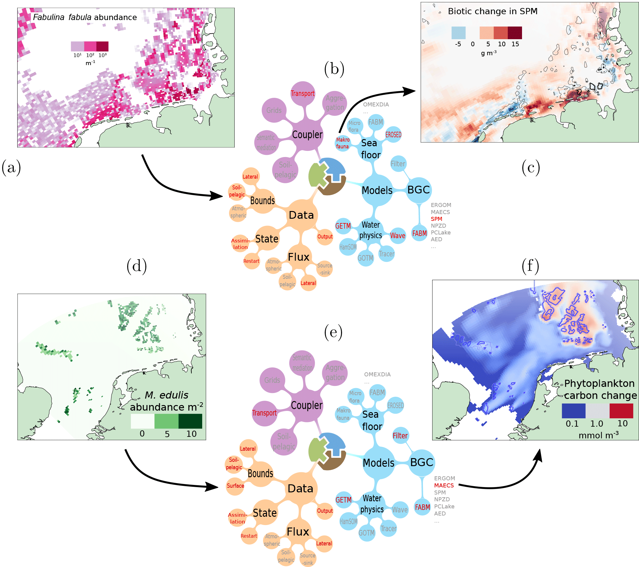
Figure 7 Building flexible applications with MOSSCO. Two bivalve-related scientific applications are showcased: Nasermoaddeli et al. (2018) investigated the effect of bottom-dwelling Fabulina fabula (a, showing parts of the southern North Sea) on suspended sediment concentration (c) with a coupled application integrating hydrodynamics, three pelagic SPM classes in the ecosystem model, the mediation of erodibility by benthic bivalves, and an explicit description of bed erosion and sedimentation (b); see Sect. 4.4 and Fig. 5. Slavik et al. (2018) investigated the effect of epistructural Mytilus edulis (d) on phytoplankton concentration (f) with a coupled application integrating hydrodynamics, the FABM–MAECS ecosystem model, and filtration by mussels (e).

A southern North Sea (SNS) domain was used in two studies concerning the effects of bivalves on the pelagic ecosystem. Slavik et al. (2018) investigated how the accumulation of epifauna on wind turbine structures (Fig. 7d) impacts pelagic primary production and ecosystem functioning in the SNS on larger spatial scales. This study is the first of its kind that extrapolates the ecosystem impacts of anthropogenic offshore wind farm structures from a local to a regional sea scale. The authors use a MOSSCO coupled system consisting of the hydrodynamic model GETM, the ecosystem model MAECS as described by Kerimoglu et al. (2017), the transport connector, the filter feeder component, and several input and output components (Fig. 7e). They assess the impact of anthropogenically enhanced filtration from blue mussel (Mytilus edulis) settlement on offshore wind farms that are planned to meet the 40-fold increase in offshore wind electricity in the European Union by 2030. They find a small but non-negligible large-scale effect in both phytoplankton stock and primary production, which possibly contributes to better water clarity (Fig. 7f).

Biological activities of macrofauna on the sea floor mediate suspended sediment dynamics, at least locally. In the study by Nasermoaddeli et al. (2018), the large-scale biological contribution of benthic macrofauna, represented by the key species Fabulina fabula (Fig. 7a), to the suspension of sediment was investigated. Simulation results for a typical winter month revealed that SPM is increased not only locally but beyond the mussel-inhabited zones. This effect is not limited to the near-bed water layers but can be observed throughout the entire water column, especially during storm events (Fig. 7c). In this coupled application, the hydrodynamic model GETM, the pelagic ecosystem component with three SPM size classes, the erosion–sedimentation and benthic mediation components, several input and one output components, and the transport connector were used (Fig. 7d).

4.4 Exemplary workflow

For the SPM bivalve example above (Nasermoaddeli et al., 2018 and Fig. 7c), the coupled system contains 13 modular components: the hydrodynamic getm_component and simplewave_component, a pelagic fabm_component, the benthic erosion–sedimentation erosed_component and benthos_component, one output and four input components, the default link_connector, the nudge_connector, and the transport_connector. Each of these 13 components is involved in at least one pairwise coupling described in a couplings section of the YAML coupling configuration (Fig. 3b). This coupled application is to be deployed in sequential mode on the same set of computing resources for all 13 components.

The horizontal spatial representation and domain decomposition are provided by the grid that is created in the hydrodynamic model and that is communicated to the wave, pelagic ecosystem, benthic, and input components; this is achieved by specifying the hydrodynamic model as a dependency of these components (dependencies in Fig. 3b) Four instances of the netcdf_input_component (see Sect. 3.2.2 and instances in Fig. 3b) are created to provide macrofauna forcing, lateral open ocean boundaries, rivers fluxes, and restart information from netCDF files. In the first of two initialisation phases, the output components and the hydrodynamic component are initialised first, as they have no dependencies. Dependent components then receive the spatial grid information from the hydrodynamic component. All components advertise what information they can provide (e.g. a certain quantity) and what information they need (e.g. grid information) in the coupled system.

In the second initialisation phase, the transport_connector ensures that all fields from the ecosystem component are made available in the hydrodynamic component for advection and diffusion. For all other pairwise couplings, the link_connector communicates advertised data from a sending component as a pointer to the receiving component; passing pointers to data instead of copies of the data is only possible in sequential mode and on identical grids. In the restart phase, additional initialisation data are communicated to all components implementing this (optional) phase; here, the bed mass and SPM concentrations are updated in the ecosystem and erosion components via a coupling to an instance of the input component that reads data from a file created in prior model runs (“restart”).

In the run phase, all pairwise couplings are called in the same order as during the initialisation phase. First, the connector (or coupler) is called to synchronise the two components' data, then each of the coupled components in this pairwise coupling is executed for the minimum time interval to the next coupling time step of the involved components (see Fig. 2). With the boundary conditions read with the input component from files at each coupling interval, the SPM fields that reside in the ecosystem component are updated by way of connecting these components with the nudge_connector. Finally, at the end of a simulation, all output components are run once more to ensure that the final state of the system is recorded; then, all components go through their finalisation phase and clean up reserved memory.

5 Discussion and outlook

In merging existing frameworks that address distinct types of modularity and by developing a superstructure for making the multi-level coupling approach applicable in coastal research, the MOSSCO system largely meets the design goals of flexibility and equitability. In doing so, the structural deficiencies of legacy models and the need for practical compromises became very apparent.

For legacy reasons, equitability is the harder to achieve design goal. Both the distribution of computing resources and the spatial grid definition can in principle be determined by any one of the participating components; de facto, in marine or aquatic research, they are prescribed by the hydrodynamic models that have so far not been enabled to inherit a grid specification or a resource distribution from a coupler or coupled system. With the ongoing development and diversification of hydrodynamic models and no immediate benefit for the different physical models to outsource grid and resource allocation, this situation is not likely to change. MOSSCO compromises here with its flexible grid inheritance scheme and with the grid-provisioning component that delivers this information to the coupled system whenever a hydrodynamic component is not used.

Beyond grid and resource allocation, however, the equitability concept is successfully driving independent developments of sub-modules. We found that experts in one particular model, e.g. the erosion module, could rely on the functionality of the other parts of the system without having to be experts themselves in all of the constituent models in the coupled application. The limitations to this black-box approach became evident in the scientific application and evaluation of the coupled model system, which was only possible when collaboration with experts in these other model systems was sought. By taking away the inaccessibility barrier and by enforcing a clear separation of tasks, the modular system stimulated a successful collaboration. Sustained granularity also helped in terms of alignment with ongoing development in external packages. These can be integrated fast into the coupled system, which does not rely on specific versions of the externally provided software unless structural changes occur. Long-term supported interfaces on the external model side facilitate MOSSCO being up to date with, for example, the fast-evolving GETM and FABM code bases.

When legacy codes were equipped with a framework–agnostic interface, we encountered four major difficulties.

1. For organising the data flow between the components, MOSSCO uses standard names and units compatible with the infrastructure and library of standard names and units provided in the pelagic component for the FABM framework (mostly modelled on CF). Other components, such as the BMIs of wrapped legacy models, do not provide such a standard name in their own implementation and, in particular, often do not adhere to a naming standard. We found ambiguity arising, e.g. with temperature to be represented as temperature vs. sea_water_temperature vs. temperature_in_water. While this can be resolved based on CF for temperature, most ecological and biogeochemical quantities currently lack a consistent naming scheme. The forthcoming GSN ontology (building on CSDMS names; Peckham, 2014) could adequately address this coupling challenge.

2. Deep subroutine hierarchies of existing models made it difficult to isolate desired functionality from the structural external overhead. In one example, in which a single functional module was taken out of the context of an existing third-party coupled system, the module depended on many routines dispersed throughout that third-party system repository.

3. Components based on stand-alone models are developed and tested with their own I/O infrastructure and typically supply a BMI implementation only for part of their state and input data fields. A new coupled application or data provisioning and/or requesting within a coupled system can therefore easily require a change in a model BMI. The implementation potential input and output for all quantities, including replacement of the entire model-specific I/O in the BMI, is therefore desirable for new developments and re-factoring.

4. Mass and energy need to be conserved across the coupled components. Mediators communicate conservatively regridded mass and energy fluxes into pairs of coupled components. These fluxes then need to be appropriately integrated by the coupled components, even when their internal time discretisation differs and for asynchronous scheduling that can incur different coupling time steps. The conservative integration of exchanged mass and energy fluxes cannot automatically be ensured by the coupling system, and the user has to carefully consider time steps in the preparation of the coupling set-up.

Efforts to make legacy models coupleable, either for MOSSCO or similar frameworks, however, can have additional benefits besides the immediate applicability in an integrated context. Coupleability strictly demands the communication of sufficient metadata, which stimulates the quality and quantity of documentation and the scientific and technical reproducibility of legacy models. Indeed, transparency has been greatly increased by wrapping legacy models in the MOSSO context. All participating components performed the introspection and leveraging of a collection of metadata at the assembly time of the coupled application and during output. Transparency is expected to be continuously increased by new coupling demands and more generous metadata provisioning from wrapped science models. MOSSCO is moving towards adopting the Common Information Model (CIM) that is also required by Climate Model Intercomparison Project (CMIP) participating coupled models (Eyring et al., 2016).

With a current small development base of 12 contributors, the openness concept of MOSSCO in terms of including contributions from outside the core developer team has not yet been tested; in the categorisation by de Laat (2007) internal governance with simple structure is sufficient at this size. Formally, external contributions can be included in MOSSCO by way of contributor licence agreements. The openness concept has been useful in instigating discussions about the need for explicit (and preferably open) licencing of related scientific software and data as demanded in current open science strategies (e.g. Scheliga et al., 2016).

Scalability in MOSSCO applications depends on the scalability of the coupled model components and on the potential overhead of the coupling infrastructure. Strong scaling experiments were performed with a coupled application using GETM, FABM with MAECS (≈ 20 additional transported 3-D tracers), and FABM with OMEXDIA_P, including bidirectional benthic–pelagic coupling, on Jureca (Krause and Thörnig, 2016). They show linear (perfect) scaling from 100 to 1000 cores and a small levelling-off (to 85% of perfect scaling) at 3000 cores. We have not observed a loss of computing time due to the infrastructure and superstructure overhead of ESMF, which remained below 0.1 % in the run phase of the scaling experiment. A typical operational computation speed achieved, e.g. in the bivalve wind farm application (Sect. 4.3; 175 000 grid cells), on 192 processors is 2000 computed hours per elapsed wall clock hour: such a performance allows for decadal to multi-decadal simulations. One of the identified bottlenecks (that varies strongly with the HPC system used) is data transfer from memory to disc: this will be addressed in the future by the use of parallel NetCDF and/or leveraging the XML I/O server (XIOS; Meursedoif, 2013).

Multi-component systems may also suffer from low acceptance by the research community. They are much harder to implement and maintain by individual groups, in the context of which researchers solve coastal ocean problems of a large range of complexity, from purely hydrodynamic applications via coupled hydrodynamic–sediment dynamic applications to fully coupled systems. Many academic problems focus on specific mechanisms and thus do not require the complete and fully coupled modular system such that the application of the full system might mean a large structural overhead and additional workload. There is, however, the necessity of following a holistic approach when tackling grand research questions in environmental science, such as those related to system responses to anthropogenic intervention. Yet, it is not clear whether the bottom-up approach of many interacting modular components leads to an emergent system behaviour that is desirable and exhibits new insights or whether the system gets tangled up in coupling complexity.

As evident from the test cases (Sect. 4), MOSSCO also encourages coupled applications that are far from a complete system-level description. With few coupled components, the technical threshold to getting an application running on an arbitrary system is relatively low. The user can quickly reach initial success. MOSSCO provides a full documentation, step by step recipes, and a public bug tracker; it adopts abundant error reporting from ESMF and a fail fast design that stops a coupled application as soon as a technical error is detected (Shore, 2004). Usability is especially high due to an available master script that compiles, deploys, and schedules a coupled application. To address a wide range of users, the system is designed to run on a single processor or on a user's laptop equally well as on a high-performance computer using several thousand computing nodes.

An obvious advantage of modular coupling is the opportunity to bridge the gap between different scientific disciplines. It allows in principle for the combination of, for example, hydrodynamic models from oceanography with sediment transport models from coastal engineering. Thus different experts can work on their individual models but benefit from all others' progress. This seeming advantage, however, also poses a drawback for modular coupling approaches. An initial effort which is necessary for individual models to meet the requirements of a modular modelling framework has to be invested. This will only happen if there is either urgent pressure to include specific model capabilities, which will be difficult to include otherwise, or if convincing examples of possible benefits can be presented. It cannot be expected that the coastal ocean modelling community will agree about one coupler or one way of interfacing modules, so it will still require considerable implementation work to transfer a module from one modular system to another. To solve this problem, coupling standards need to become more general, but in turn this might even increase the structural overhead involved in using these systems.

For certain applications it might be preferable for different reasons to hardwire sub-models and exercise strong control over such a monolithic coupled system. But at the least, such sub-models should be made coupleable by following the minimal requirements set forth by the BMI specification. This ensures that the monolithic model system or parts of it can be reused or expanded in a more modular way. And by strictly separating the BMI from any framework-specific CMI specification, the effort spent on wrapping an existing model or on equipping a new model with a basic model interface is not tied to a particular coupling framework or even a particular coupling framework technology. A model that follows BMI principles will be more easily interfaced to other models no matter what coupler is used. Wrapped legacy models from MOSSCO can thus be useful in non-ESMF contexts as well, and models with an existing BMI can be integrated into MOSSCO more easily in turn.

One demand for integrative modelling, which is likely best practised in open and flexible system approaches, arises from current European Union legislation. The Water Framework Directive and the Marine Strategic Planning Directive require the description of marine environmental conditions and the development of action plans to achieve a good environmental status. These objectives can initially be met by a monitoring programme to determine present-day conditions but ultimately rely on numerical model studies to evaluate anthropogenic measures. This ecosystem-based approach to management (e.g. Ruckelshaus et al., 2008) demands modelling systems which are capable of taking into account hydrodynamics, biogeochemistry, sedimentology, and their interactions to properly describe the environmental status. As further legal requirements can be expected for many coastal seas worldwide, numerical modelling systems applied for this task need to be flexible in terms of integrating additional (e.g. site-specific) processes. In this ongoing process, the initial effort of creating a modular system may be the only way forward that can take into account all relevant processes in the long run.

Outlook

The suite of components provided or encapsulated so far meets the demands that were initially formulated by our users; they already allow for a wide range of novel coupled applications to investigate the coastal sea. To stimulate more collaboration, however, and to bring forward a general “ecosystem” of modular science components, several legacy models could interface to MOSSCO components in the near future by building on complementary work at other institutions. For example, the Regional Earth System Model (RegESM; Turuncoglu et al., 2013; Turuncoglu and Sannino, 2017) provides ESMF interfaces for MITgcm, ROMS, and WAM, amongst others. The convergence of the development of MOSSCO and RegESM is feasible in the near term. Also, the recently developed Icosahedral Non-Hydrostatic Atmospheric Model (ICON; Zängl et al., 2015) is currently being equipped with an ESMF component model interface.

Once ESMF interfaces have been developed for a legacy model, it is desirable that these developments move out of the coupler system and become integrated into the development of the legacy model itself. This has been successfully achieved with the ESMF interface for the hydrodynamic model GETM, which is now distributed with the GETM code. Much of the utility layer developed in MOSSCO, or likewise in MAPL or in the ESMF extension of the WRF model, is expected to be propagated upstream into the framework ESMF itself.

The interoperability of current coupling standards will increase. While currently there are three flavours of ESMF (basic ESMF as in MOSSCO, ESMF–MAPL as in the GEOS-5 system, and ESMF–NUOPC as in the RegESM), only a minor effort would be required to provide the basic ESMF and ESMF–MAPL implementations with a NUOPC cap and make them interoperable with the entire ESMF ecosystem. Even a coupling of ESMF-based systems to OASIS-MCT-based systems has been proposed, and investigation is ongoing on a coupling of MOSSCO to the formal BMI for CSDMS.

6 Conclusions

We problematised both the primacy of hydrodynamic models and the limited modularity in coupled coastal modelling that can stand in the way of developing and applying novel and diverse biogeochemical process descriptions. Such developmental potential is likely needed to progress towards holistic regional coastal systems models. We presented the novel Modular System for Shelves and Coasts (MOSSCO) that is built on coupling concepts centred around equitability and flexibility to resolve the issue of obstructed modularity. These concepts also bring about openness, usability, transparency, and scalability. MOSSCO as a current Fortran implementation of this concept includes the wrapped Framework for Aquatic Biogeochemical Models (FABM) and a usability layer for the Earth System Modeling Framework (ESMF).

The MOSSCO design principles emphasise basic coupleability and rich meta-information. Basic coupleability requires that models communicate about flow control, computing resources, and exchanged data and metadata. We demonstrated that the design principles of flexibility and equitability enable the building of complex coupled models that adequately represent the complexity found in environmental modelling. In this first version, the MOSSCO software wrapped several existing legacy models with basic model interfaces (BMIs); we added ESMF-specific component model interfaces (CMIs) to these wrappers and other models and frameworks to build a suite of ESMF components that when coupled represent a small part of a holistic coastal system. These components deal with hydrodynamics, waves, pelagic and sediment ecology and biogeochemistry, river loads, erosion, resuspension, biotic sediment modification, and filter feeding.

In selected applications, each with a different research question, the applicability of the coupled system was successfully tested. MOSSCO facilitates the development of new coupled applications for studying coastal processes that extend from the atmosphere through the water column into the seabed and that range from laboratory studies to 3-D simulation studies of a regional sea. This system meets an infrastructural need that is defined by experimenters and process modellers who develop biogeochemical, physical, sedimentological, or ecological models on the lab scale first and who would like to seamlessly embed these models into the complex coupled three-dimensional coastal system. This upscaling procedure may ultimately also support the global Earth system community.

Appendix A: Acronyms and model abbreviations used in the text

bash	GNU Bourne Again SHell
BFM	Biogeochemical Flux Model
	(ecosystem model)
BGC	Biogeochemistry
BMI	Basic model interface (coupling concept)
CC-BY-SA	Creative Commons Attribution
	Share-Alike licence
CF	NetCDF Climate and Forecast convention
CIM	Common Information Model
	(metadata standard)
CMI	Component model interface
	(coupling concept)
CMIP	Climate Model Intercomparison Project
COAWST	Coupled Ocean–Atmosphere–Wave–
	Sediment Transport
CSDMS	Community Surface Dynamics
	Modeling System
DKRZ	Deutsches Klimarechenzentrum (HPC centre)
ESM	Earth system model
ESMF	Earth System Modeling Framework
FABM	Framework for Aquatic
	Biogeochemical Models
FMS	Flexible Modeling System
	(coupling technology)
FONA	Forschung für Nachhaltigkeit (funding scheme)
FVCOM	Finite-Volume Coastal Ocean Model
GCC	GNU Compiler Collection
GETM	General Estuarine Transport Model
	(3-D coastal ocean model)
GEOS-5	Goddard Earth Observing System version 5
GNU	GNU is Not Unix
GOTM	General Ocean Turbulence Model
	(1-D water column model)
GPL	General Public License
GSN	Geoscience Standard Names Ontology
HLRN	Norddeutscher Verbund für Hoch-
	und Höchstleistungsrechnen
HPC	High-performance computing
ICON	Icosahedral Non-Hydrostatic Model
I/O	Input and output
JSC	Jülich Supercomputing Centre
MAPL	Modeling Analysis and Prediction Layer
MAECS	Model for Adaptive Ecosystems
	in Coastal Seas
MCT	Model Coupling Toolkit
MESSy	Modular Earth Submodel System
MITgcm	Massachusetts Institute of Technology
	Global Circulation Model
MOM	Modular Ocean Model
MOSSCO	Modular System for Shelves and Coasts
MPI	Message-passing interface

MSPD	European Union Marine Strategic
	Planning Directive
NEMO	Nucleus for European Modelling
	of the Ocean
NetCDF	Network Common Data Form
NPZD	Nutrient, phytoplankton, zooplankton,
	detritus (ecosystem model)
NUOPC	National Unified Operational
	Prediction Capability
OASIS	Ocean Atmosphere Sea Ice Soil coupler
OMEXDIA	Ocean Margin Exchange Experiment
	early diagenetic model
OMEXDIA_P	OMEXDIA with added phosphorous
OMUSE	Oceanographic Multipurpose Software
	Environment
PARSE	Prepare, adapt, register, schedule,
	execute methodology
PISCES	Pelagic Interactions Scheme for
	Carbon and Ecosystem Studies
POM	Particulate organic matter
POC	Particulate organic carbon
RegESM	Regional Earth System Model
ROMS	Regional Ocean Modeling System
SCRIP	Spherical Coordinate Remapping and
	Interpolation Package
SNS	Southern North Sea
SPM	Suspended particulate matter
SWAN	Simulating Waves Nearshore
WAM	Wave atmospheric model
WFD	European Union Water Framework
	Directive
WRF	Advanced Research Weather
	Research and Forecasting
XIOS	XML input–output server
XML	Extensible Markup Language
YAML	YAML Ain't Markup Language