Description and validation of the Simple, Efficient, Dynamic, Global, Ecological Simulator (SEDGES v.1.0)

In this paper, we present a simple dynamic global vegetation model whose primary intended use is auxiliary to the land–atmosphere coupling scheme of a climate model, particularly one of intermediate complexity. The model simulates and provides important ecological-only variables but also some hydrological and surface energy variables that are typically either simulated by land surface schemes or else used as boundary data input for these schemes. The model formulations and their derivations are presented here, in detail. The model includes some realistic and useful features for its level of complexity, including a photosynthetic dependency on light, full coupling of photosynthesis and transpiration through an interactive canopy resistance, and a soil organic carbon dependence for bare-soil albedo. We evaluate the model's performance by running it as part of a simple land surface scheme that is driven by reanalysis data. The evaluation against observational data includes net primary productivity, leaf area index, surface albedo, and diagnosed variables relevant for the closure of the hydrological cycle. In this setup, we find that the model gives an adequate to good simulation of basic large-scale ecological and hydrological variables. Of the variables analyzed in this paper, gross primary productivity is particularly well simulated. The results also reveal the current limitations of the model. The most significant deficiency is the excessive simulation of evapotranspiration in mid- to high northern latitudes during their winter to spring transition. The model has a relative advantage in situations that require some combination of computational efficiency, model transparency and tractability, and the simulation of the large-scale vegetation and land surface characteristics under non-present-day conditions.

1 Introduction

Simulation of the land surface is a critical component of models of the Earth climate system. In such models, heat, energy, and moisture transfer between the land and atmosphere or ocean are calculated with information from the hydrological and vegetation components of these models. The Simple, Efficient, Dynamic, Global, Ecological Simulator (SEDGES) simulates the gross properties of vegetation, as well as some large-scale land surface characteristics, which are important for the simulation of energy and moisture exchange with the atmosphere. These simulated variables are to be used by a land surface scheme in which SEDGES is embedded in a climate or Earth system model. Models of similar complexity to SEDGES exist that simulate the vegetative if not also the hydrological and energy-transferring aspects of the land surface, include the Vegetation Continuous Description model (VECODE) (Brovkin et al., 1997, 2002) and the Efficient Numerical Terrestrial Scheme (ENTS) (Williamson et al., 2006). The purpose of these kinds of models is to efficiently and reasonably simulate dynamic land surface characteristics and behavior and provide these to the atmospheric components of Earth system models of intermediate complexity. In such a framework, the need for sophisticated simulations of the land surface is obviated by the simplifications present in the other model components (which reduce the benefit of a more realistic representations of land surface processes as compared to when the other model components are complex and realistic), by a desire to more easily understand the processes underlying experimental results, and by the computational burden that goes along with the increased complexity.

SEDGES is a new model that is based on the original SIMulator for Biospheric Aspects (SimBA) model (Kleidon, 2006b), which is coupled to the Planet Simulator (PlaSim) general circulation model (GCM) (Lunkeit et al., 2007), and it is even more strongly based on a later version of SimBA that the lead author of this paper developed (Lunkeit et al., 2011) and which is also coupled to PlaSim. Neither version of SimBA has been thoroughly evaluated. However, when coupled to PlaSim, the earlier version's net primary productivity was shown to be broadly reasonable in Kleidon (2006b), and it has been used successfully in a number of studies (e.g., Kleidon, 2006a, b; Bowring et al., 2014). The SimBA model is based on a light and water-use efficiency model for crops (Monteith et al., 1989) that was later adapted and expanded to forest canopies (Dewar, 1997). This approach to vegetative productivity is maintained in SEDGES and helps form the core of the model. Other aspects of SEDGES's structure that are particular to SEDGES (i.e., are uncommon in or absent from other models) are carried over from the original SimBA, including the determination of soil water-holding capacity and moist-soil leaf cover fraction by the amount of vegetation biomass (Fig. 1).

SEDGES builds upon SimBA by improving most of its parameterizations. Some of the updated and expanded model features are taken or adapted from currently existing models. Although SEDGES makes many improvements upon the original SimBA, it is still a simple model; i.e., it is not of “intermediate” complexity (cf. Willeit and Ganopolski, 2016). Compared to the original SimBA, SEDGES (and the land surface framework that it presupposes) has four major increases in complexity: the separation of evapotranspiration into soil and vegetative components, the inclusion of aerodynamic conductance in the formulation for carbon uptake by vegetation, full coupling of photosynthesis and transpiration through interactive canopy conductance, and soil organic carbon-dependent soil albedo. Choosing the appropriate level of complexity of represented processes within a land surface or dynamic global vegetation model often depends on the context in which the model is to be used and involves subjective weighting of trade-offs between increased accuracy and realism on the one hand and, on the other hand, robustness to the chosen values of poorly constrained parameters and model reliability in a wide range of situations (Prentice et al., 2015).

This paper presents the SEDGES model's structure, equations, and ability to simulate ecological and hydrological variables when used in conjunction with a simple soil hydrological scheme and parameterization for aerodynamic conductance and forced by reanalysis data.

2 Model description: SEDGES

2.1 Overview of SEDGES

SEDGES is a simple, dynamic global vegetation model (DGVM). Within the context of the history of land surface modeling, the SEDGES framework (defined as SEDGES and the type of land surface model that it presupposes that it forms a part of) combines aspects of first- and third-generation models (Sellers et al., 1997; Pitman, 2003; Prentice et al., 2015), which include, respectively, the use of a simple single-layer “bucket” model for soil hydrology and the full coupling of photosynthesis and transpiration through interactive canopy conductance.

The intended main use of SEDGES is for it to be embedded within a land surface scheme and to thus help the land surface scheme simulate large-scale properties and behavior of the surface in which vegetation and soil play a role. These large-scale properties and behavior include interactions between the land surface and the atmosphere through simulated CO₂, moisture, energy, heat, and momentum exchanges. SEDGES either directly simulates or else provides the greater land surface scheme with the necessary variables. SEDGES also simulates ecological variables (e.g., biomass, soil organic carbon, forest cover fraction, leaf cover fraction) that are not directly used outside it by either the rest of the land surface scheme or by the atmosphere, but these ecological variables almost always have a downstream impact on the simulations of the aforementioned land–atmosphere exchanges. SEDGES has been designed, in particular, for coupling with the Planet Simulator, and thus presupposes that the land surface scheme that it forms a part of be similar to that of PlaSim in its hydrology and scheme for surface evaporation. This section presents, in detail, the SEDGES model formulations for its output ecological and land surface variables, including their derivations.

Overall, sub-grid-scale heterogeneity is treated similarly in SEDGES as it is in the SLAM-1T (Simple Land-Atmosphere Mosaic – 1 Tile) configuration of CHASM (CHAmeleon Surface Model) (Desborough, 1999) and in the original Met Office Surface Exchange Scheme (MOSES) land surface scheme (Cox et al., 1999). Because of its need to couple with the Planet Simulator GCM, which uses a bulk aerodynamic formulation with a single tile (i.e., one surface type per grid cell), SEDGES handles sub-grid-scale heterogeneity according to what is called the “average parameter” method (Giorgi and Avissar, 1997) or the “composite” approach (Li and Arora, 2012; Melton and Arora, 2014). In this approach, land surface characteristics are aggregated to provide a single, representative value on the scale of the entire grid cell. The framework in SEDGES for evapotranspiration (ET) is special because it also qualifies as a simplified mosaic (or “mixed”, Li and Arora, 2012) approach, such that only surface conductance differs between the surface types (or tiles). This mosaic approach is also used to extend a “big-leaf” formulation for vegetative CO₂ uptake (Appendix B of Raupach, 1998) to a mixed soil–vegetation surface, enabling us to isolate the fraction of total ET that is due to transpiration and thus formulate vegetative control of water loss and CO₂ uptake. The SEDGES framework neglects evaporation from intercepted canopy water and thus only distinguishes between two tiles when snow is absent: bare soil and vegetation. When there is snow cover, there are essentially three tiles: snow-free exposed bare soil, snow-covered surface, and snow-free exposed vegetation (see Sect. 2.3.1 for more detail).

Figure 2 Canopy resistance dependencies and updating in SEDGES

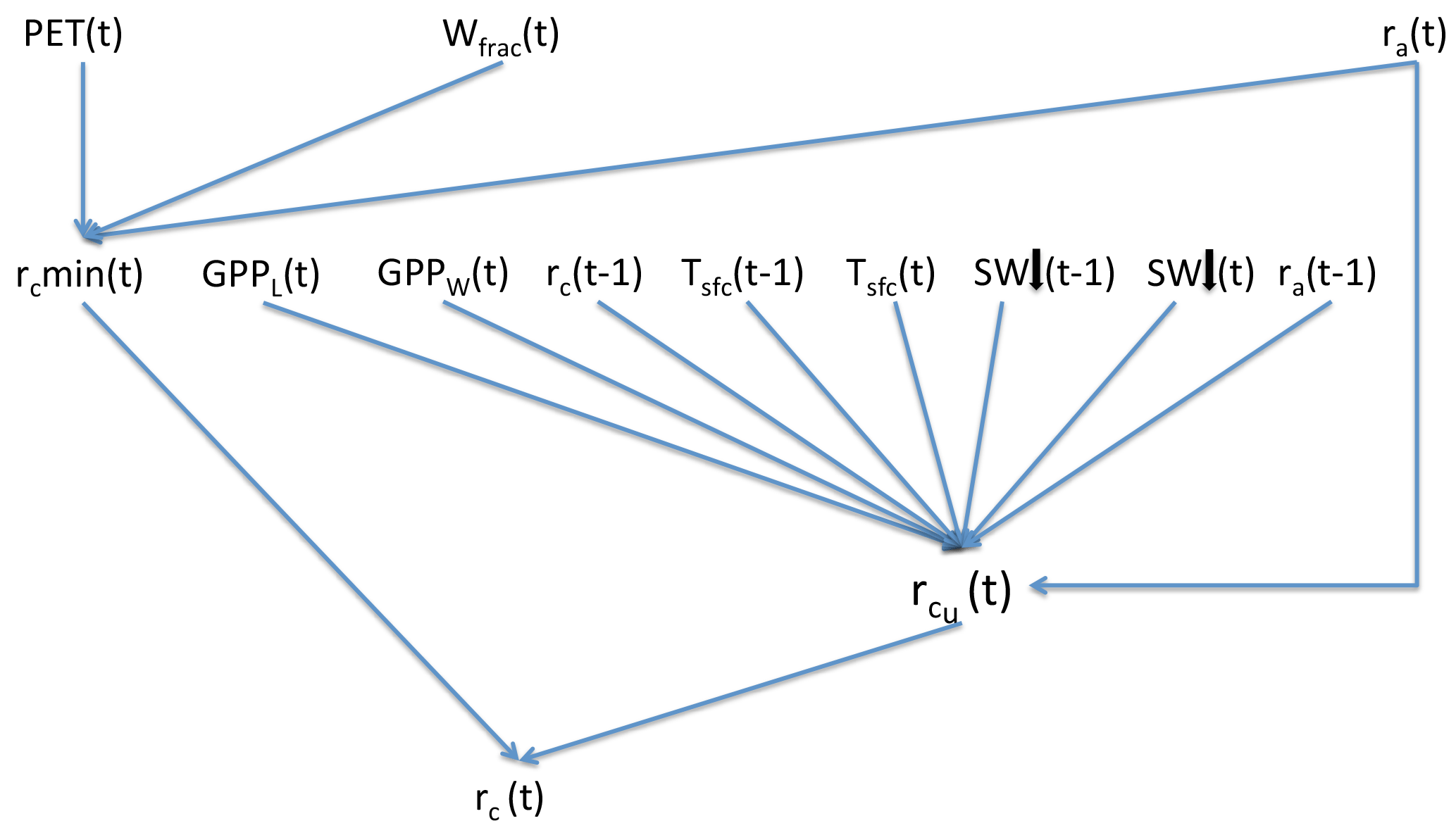
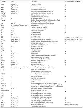
Table 1 SEDGES variables in the paper. Notation for the rightmost column is as follows: “I”, “O”, and “M” indicate variables that are, respectively, input to, output by, or modified by the SEDGES model. A blank field in that column indicates that the variable could be output if desired, but some code changes would be needed. “EI” denotes a variable from ERA-Interim that is used by the simple land surface scheme that we use to drive SEDGES with in Sect. 4. We denote by “M” only those output variables that are output by SEDGES that are expected to be already existing in the land surface scheme in which SEDGES is embedded.

Franks et al. (2013)Pisek et al. (2010); He et al. (2012)Raupach (1998)van de Griend and Owe (1994)Knorr (2000)Jenkinson et al. (1990)Roesch et al. (2001)Roeckner et al. (2003)Moody et al. (2007)Oke (1987)(Sellers et al., 1996b)

Table 2 SEDGES parameters in the paper.

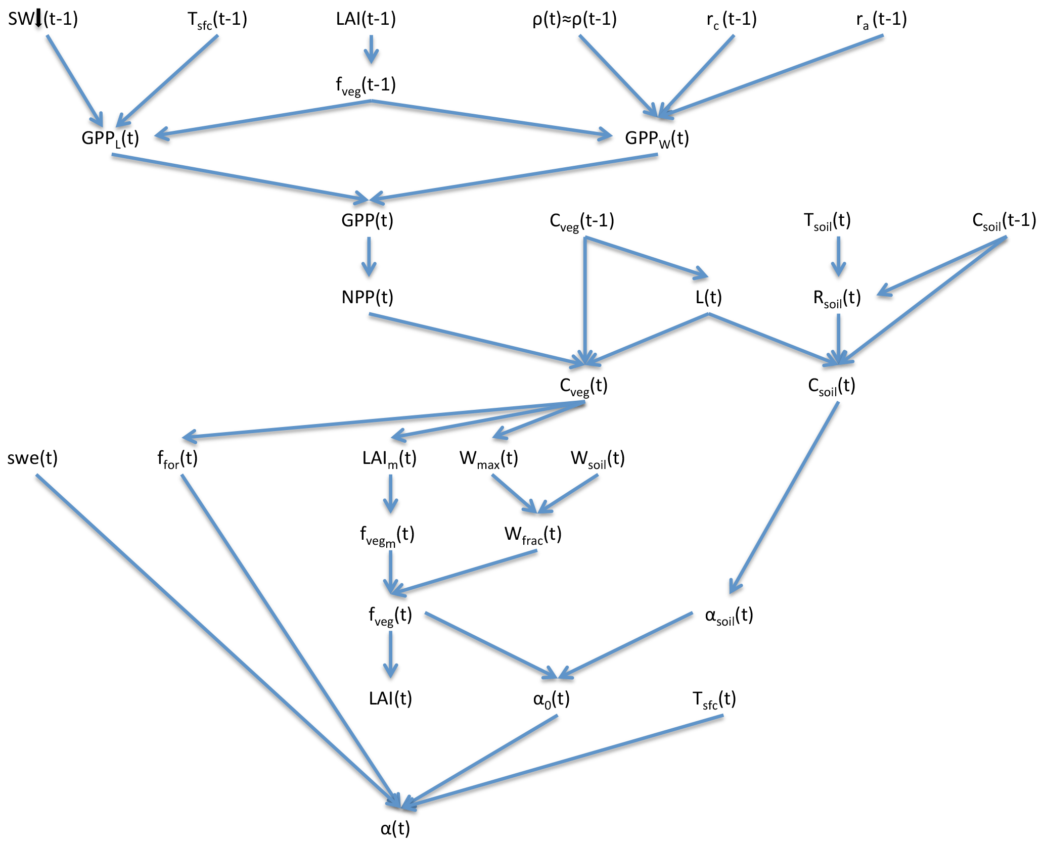
The core driving variable in SEDGES is gross primary productivity (GPP), which impacts the living biomass, which, in turn, heavily influences or determines the values of almost every other simulated land surface variable (listed in Sect. 3). Forest cover and leaf cover fractions and (implicitly) rooting depth are parameterized to increase with biomass using respective relationships that are fixed. SEDGES (as well as SimBA) uses a simple single-layer bucket for the soil hydrology and has essentially one plant functional type. Soil organic carbon is treated as a single homogeneous reservoir. Surface albedo depends on soil organic carbon content, snow depth, biomass, and leaf cover fraction. Surface roughness increases monotonically with biomass. Gross primary productivity and canopy resistance¹ are coupled through the vegetation's effort to conjointly minimize water loss and satisfy photosynthetic demand for CO₂, as per the original Dewar (1997) model (see Sect. 2.2.6). Table 1 lists all SEDGES variables, their units, and their relationship with the SEDGES vegetation model. Their dependencies and how those variables are updated is shown in Figs. 1 and 2. Table 2 lists all parameters that are used in the paper along with their values and their units.

With its main use and design already indicated, SEDGES can also be forced offline with external data. The offline mode of SEDGES was used in combination with a simple soil hydrological scheme and parameterization for aerodynamic conductance and run using reanalysis climate data for the SEDGES model evaluation (see Sect. 4).

In Sect. 2.2 and 2.3, we describe in detail the equations of the ecological and physical variables in the SEDGES model. Because SEDGES uses the original SimBA model (Kleidon, 2006b) (and its code) as a basis, we explicitly mention in the text when significant changes are introduced in SEDGES compared with SimBA. We provide extra detail on the original SimBA for the cases in which Kleidon (2006b) provides insufficient information for comparison with SEDGES. The broadest structural increases in complexity in SEDGES have already been identified in the introduction; our focuses are narrower in scope in these coming sections.

2.2 Equations for ecological variables

2.2.1 Vegetation biomass

The most important SEDGES variable is biomass of live vegetation. This quantity is used to directly or indirectly derive almost all the land surface variables; these are presented in the coming sections. The prognostic equation for biomass is as follows:

$$\begin{array}{}\text{(1)}& {\displaystyle \frac{{\mathrm{dC}}_{\mathrm{veg}}}{\mathrm{d}t}}=\mathrm{NPP}-L,\end{array}$$

where C_veg is the carbon in living biomass (kg C m⁻²), L is the litterfall and equals $\frac{{\mathrm{C}}_{\mathrm{veg}}}{{\mathit{\tau }}_{\mathrm{veg}}}$, τ_veg is the residence time of the vegetative carbon (see Sect. 2.2.9) and equals 10 years, and NPP (net primary productivity) is approximated as 0.5 GPP.

2.2.2 Net primary productivity and gross primary productivity

SEDGES uses a constant NPP ∕ GPP = 0.5 approximation. This approximation is supported by the conservative nature of the ratio of mitochondrial respiration to gross photosynthesis and (hence) of the ratio of net photosynthesis to gross photosynthesis over a wide variety of conditions, on timescales of weeks or more (see the brief review in Van Oijen et al., 2010). Since each model time step in SEDGES is much shorter than this, it thus might seem incorrect to hold NPP ∕ GPP fixed for each time step. It is appropriate to do so, however, because the NPP-to-GPP ratio in SEDGES only impacts biomass changes, and the latter occur on very long timescales. Finally, meta-analyses of previous studies have found a robust (DeLucia et al., 2007; Litton et al., 2007) linear or proportional relationship between NPP and GPP, with slope or proportionality constant of around 0.5 (Gifford, 2003; DeLucia et al., 2007; Litton et al., 2007), albeit with considerable variation in NPP ∕ GPP across field sites (Amthor and Baldocchi, 2001; DeLucia et al., 2007; Litton et al., 2007).

GPP is calculated as the minimum of a light-limited rate, GPP_L, and a water-limited rate, GPP_W (Monteith et al., 1989; Dewar, 1997). That is, GPP $=min({\mathrm{GPP}}_{\mathrm{L}},{\mathrm{GPP}}_{\mathrm{W}}$.)

2.2.3 Light-limited gross primary productivity

GPP_L uses a light use efficiency (LUE) formulation (e.g., Yuan et al., 2007) whose overall structure is very similar to that of the original version of SimBA (Kleidon, 2006b). The equation is as follows:

$$\begin{array}{}\text{(2)}& {\mathrm{GPP}}_{\mathrm{L}}={\mathit{ϵ}}_{max}\cdot f_{\mathrm{1}}\left({\mathrm{CO}}_{\mathrm{2}}\right)\cdot f_{\mathrm{2}}\left(T_{\mathrm{sfc}}\right)\cdot f_{\mathrm{APAR}}\cdot \mathrm{SW}\downarrow ,\end{array}$$

where ϵ_max is a globally constant maximum LUE parameter ($\mathrm{5.0}\times {\mathrm{10}}^{-\mathrm{10}}$ kg C J⁻¹); f₁(CO₂) is a CO₂ fertilization function (described below); f₂(T_sfc) is a temperature limitation function (described below); f_APAR is the fraction of photosynthetically active radiation (PAR) that is absorbed by green vegetation (see below); and SW↓ is the downward flux of shortwave radiation just above the canopy surface (in W m⁻²). (Instead of this term, the original version of SimBA (Kleidon, 2006b) uses the net surface shortwave radiation flux.)

In Eq. (2), the first term on the right-hand side, ϵ_max, is the LUE with respect to the total shortwave broadband radiation that is absorbed by the photosynthetic parts of the vegetation. This constant term is the maximum efficiency with which incident shortwave radiation can be used to synthesize vegetative carbon at the reference (360 ppmv) CO₂ level (also see explanation of f_APAR, below).

The second term in Eq. (2), f₁(CO₂), increases productivity with increasing CO₂ and is taken directly from Eq. (5) of Franks et al. (2013). For CO${}_{\mathrm{2}}>{\mathrm{CO}}_{{\mathrm{2}}_{\mathrm{comp}}}$, we have

$$\begin{array}{}\text{(3)}& f_{\mathrm{1}}\left({\mathrm{CO}}_{\mathrm{2}}\right)={{\mathrm{CO}}_{\mathrm{2}}}_{\mathrm{norm}}{\displaystyle \frac{c_{\mathrm{a}}-{\mathrm{CO}}_{{\mathrm{2}}_{\mathrm{comp}}}}{c_{\mathrm{a}}+\mathrm{2}{\mathrm{CO}}_{{\mathrm{2}}_{\mathrm{comp}}}}},\end{array}$$

where c_a is the atmospheric CO₂ concentration (ppmv), ${\mathrm{CO}}_{{\mathrm{2}}_{\mathrm{comp}}}=\mathrm{40}$ ppmv is the light compensation point in the absence of dark respiration, and ${{\mathrm{CO}}_{\mathrm{2}}}_{\mathrm{norm}}=\frac{\mathrm{360}+\mathrm{2}{\mathrm{CO}}_{{\mathrm{2}}_{\mathrm{comp}}}}{\mathrm{360}-{\mathrm{CO}}_{{\mathrm{2}}_{\mathrm{comp}}}}$. Otherwise, f₁(CO₂)=0. This fertilization function replaces an earlier “beta” factor approach used in SimBA (Lunkeit et al., 2011). The latter does not saturate and therefore yields unrealistically large fertilization at high CO₂ levels.

The third term in Eq. (2) is f₂(T_sfc). f₂(T_sfc) is a ramp function, reducing productivity linearly from a surface temperature of T_crit≡20 to 0 ^∘C, with f₂(T_sfc)=0 for below 0 ^∘C temperatures. The 20 ^∘C value is the critical temperature below which productivity drops. See Appendix Appendix A for more discussion.

The fourth term in Eq. (2) is f_APAR. “f_APAR” refers to the fraction of PAR that is absorbed by photosynthesizing parts (i.e., green leaves) of plants. PAR is the portion (≈ 50 %) of incoming solar radiation that is in wavelengths usable for photosynthesis. We approximate f_APAR as follows:

$$\begin{array}{}\text{(4)}& f_{\mathrm{APAR}}=\mathrm{1}-e^{-k_{\mathrm{veg}}\cdot {\mathrm{\Omega }}_{\mathrm{c}}\cdot \mathrm{LAI}},\end{array}$$

where k_veg is a light extinction coefficient (set to 1 for horizontal leaves), Ω_c is the clumping index (or factor) and is set to 0.7, a near-mean value for natural land cover types (Pisek et al., 2010; He et al., 2012), and LAI is the leaf area index (see Sect. 2.2.8).

Equation (4) uses a simple Beer–Lambert approach, extended to canopies with leaves that are nonrandomly distributed in space (Nilson, 1971) (e.g., “clumped”). Here, we have used the common approximation (e.g., see Gower et al., 1999) that f_APAR equals the fraction of intercepted PAR (f_IPAR). Other assumptions and simplifications in Eq. (4) include an azimuthally symmetric leaf distribution (Gower et al., 1999), leaf absorptivity of 1 with respect to PAR, and the neglect of the influence of non-photosynthesizing plant parts. A final and important assumption of horizontal leaves² eliminates zenith angle dependency of the light extinction coefficient (Campbell and Norman, 1998), which makes the canopy gap fraction the same from any angle. This, in turn, eliminates the dependency of f_IPAR on diffusive/direct radiative partitioning and on zenith angle, thus reducing f_IPAR (and f_APAR) to the simple Beer–Lambert expression of Eq. (4), with a constant light extinction coefficient. Earlier versions of SimBA and the derivative model (Dewar, 1997) assume a constant value of 0.5 for k_veg.

The simplifications made in the last paragraph allow us to interchange f_APAR and the leaf cover fraction, f_leaf. Thus, we can rewrite Eq. (4) as follows:

$$\begin{array}{}\text{(5)}& f_{\mathrm{leaf}}=\mathrm{1}-e^{-k_{\mathrm{veg}}\cdot {\mathrm{\Omega }}_{\mathrm{c}}\cdot \mathrm{LAI}},\end{array}$$

where f_leaf is the areal fraction of view that is covered by photosynthesizing plant parts when looking directly down on the land surface. That is, $f_{\mathrm{leaf}}=\mathrm{1}-$ the gap fraction from the nadir.

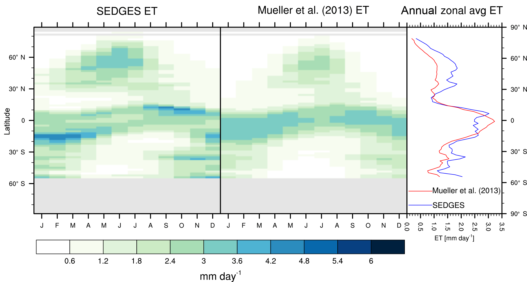
Figure 3 Zonal multiyear monthly means and zonal multiyear annual means of ET for SEDGES and the Mueller et al. (2013) reference dataset for the 1989–2005 period over non-glaciated land.

2.2.4 Water-limited gross primary productivity

Most land plants take up the CO₂ they need for photosynthesis through tiny pores in their leaves called “stomata”. Water is also lost (transpired) through these same openings. Water loss in excess of water uptake can lead to cavitation, hydraulic system collapse (e.g., see discussion in Sperry et al., 2002), and/or permanent reduction in photosynthetic capacity (Lawlor and Cornic, 2002). To prevent and mitigate such occurrences in both the present and future, most land plants adjust their stomatal openings in such a way as to balance the short- and long-term costs of transpiration with the photosynthetic gain from increased CO₂ intake (Cowan and Farquhar, 1977; Medlyn et al., 2011; Buckley and Schymanski, 2014; Prentice et al., 2014). Thus, water limitation in most land plants is closely tied to CO₂ limitation on photosynthesis. For this reason, this CO₂-limited rate in SEDGES is referred to as the “water-limited rate of GPP”. This rate is given as follows:

$$\begin{array}{}\text{(6)}& {\mathrm{GPP}}_{\mathrm{W}}={\displaystyle \frac{\left(\mathrm{co}\mathrm{2}\mathrm{conv}\right)\left(\mathrm{1}-\frac{c_{\mathrm{i}}}{c_{\mathrm{a}}}\right)c_{\mathrm{a}}\left(f_{\mathrm{leaf}}\right)\mathit{\rho }}{\mathrm{1.6}{r}_{\mathrm{c}}+r_{\mathrm{a}}}},\end{array}$$

where r_c is the canopy resistance (see Sect. 2.2.6); r_a is the aerodynamic resistance; $\mathit{\rho }\left(\equiv \frac{p_{\mathrm{sfc}}}{R_{\mathrm{d}}{T}_{\mathrm{sfc}}}\right)$ is the surface air density, where p_sfc is the surface pressure and R_d is the gas constant for dry air; co2conv $=\mathrm{4.15}\times {\mathrm{10}}^{-\mathrm{7}}$ kg C kg air⁻¹ ppmv⁻¹; c_i represents a “bulk leaf” intercellular concentration of CO₂ (ppmv); and $\frac{c_{\mathrm{i}}}{c_{\mathrm{a}}}$ is set to 0.80. This last value was lowered from the ≈ 0.86 value that was apparently used in Raupach (1998) because such a high value is less representative of typical daytime $\frac{c_{\mathrm{i}}}{c_{\mathrm{a}}}$ values (e.g., see Prentice et al., 2014). SimBA uses a value of 0.7. The ramifications of using a fixed value of $\frac{c_{\mathrm{i}}}{c_{\mathrm{a}}}$ are discussed in Sect. 6.

Equation (6) is essentially the bulk aerodynamic formula for CO₂ in Appendix B of Raupach (1998), except that we have multiplied their right-hand side by f_leaf to generalize from their big-leaf approach to the simplified mosaic framework (as mentioned in Sect. 2.1), and we have multiplied by the ratio of the molar masses of carbon and CO₂ to convert the flux into carbon units. In addition, we neglect the contribution of leaf mitochondrial respiration for simplicity. (It can be shown that including daytime leaf mitochondrial respiration in the formulation of GPP_W multiplies its current form by a factor of $\frac{\mathrm{1}}{\mathrm{1}-X}$, where X is the ratio of leaf mitochondrial respiration under light to gross photosynthesis.)

The above bulk aerodynamic formulation for GPP_W in SEDGES is more realistic than the diffusive scheme used in earlier versions of SimBA and in the Dewar (1997) model. The latter scheme, at the canopy level, assumes that r_c ≫ r_a (which is noted, too, by Medlyn et al., 2017). This condition is likely to be satisfied for aerodynamically rough canopies and when using daily-averaged environmental conditions, such as in Dewar (1997). However, early diagnostic tests of SEDGES coupled with PlaSim showed that the condition was often not satisfied, thus motivating our implementation of the bulk aerodynamic formulation for CO₂ uptake. Implementing the new formulation led to higher daytime values of r_c for moist areas (which is shown by Medlyn et al., 2017, to follow from theory). These values were more in line with reported maximum surface conductances for various vegetation types (Kelliher et al., 1995). Use of the bulk aerodynamic formulation for GPP_W also unifies vegetation–atmosphere exchanges of CO₂ and water under the same physical framework, which enables the process of transpiration to be properly tied into carbon uptake through interactive canopy conductance (see Sect. 2.2.6).

2.2.5 Evapotranspiration and transpiration

As was mentioned earlier in Sect. 2.1, the SEDGES framework for ET is very similar to the approaches taken by the SLAM-1T configuration of CHASM (Desborough, 1999) and by the original MOSES land surface scheme (Cox et al., 1999). These approaches all expand on the SimBA framework (Appendix Appendix C) by separating evapotranspiration into soil and vegetative components and (in SEDGES and MOSES) by coupling photosynthesis and transpiration through interactive canopy conductance. We find that these changes greatly improve the simulation of ET (compare Fig. A2 with Fig. 3) when using the forcing setup described in Sect. 4.

By design, SEDGES does not directly calculate the evapotranspiration; rather, it provides a surface wetness factor to be used by the bulk aerodynamic formulation of the land surface scheme that is coupled to the atmospheric model, which performs the actual calculation of ET. An exception to this exporting of ET calculation to outside of SEDGES is the explicit calculation by SEDGES of evaporation from exposed soil when there is snow cover.

Although the (total) evapotranspiration is calculated outside of SEDGES, the way it is simulated is intimately tied into many parameterizations within the actual SEDGES model, which presuppose a specific ET framework (as discussed in Sects. 2.1 and 3). The ET framework is thus presented in this section, along with the SEDGES parameterizations that help comprise it. For this simplified mosaic approach (Sect. 2.1), we remind the reader that the aerodynamic conductance and saturation specific humidity of the air at the surface are homogeneous throughout the grid cell:³

$$\begin{array}{}\text{(7)}& \mathrm{ET}={\displaystyle \frac{\mathit{\rho }}{{\mathit{\rho }}_{\mathrm{w}}{r}_{\mathrm{a}}}}{\mathrm{C}}_{\mathrm{w}}\mathrm{\Delta }q,\end{array}$$

where ET is the evapotranspiration in units of volumetric liquid water m³ m⁻² s⁻¹, ρ_w is the density of liquid water, $\mathrm{\Delta }q\equiv q{\mathrm{sat}}_{\mathrm{sfc}}-q$, qsat_sfc is the temperature- (T_sfc) and pressure- (p_sfc) dependent saturation specific humidity of the air at the surface, q is the specific humidity of the air at the lowest atmospheric model level, and C_w is a surface “wetness” factor that reduces evapotranspiration from the potential rate by incorporating the effects of canopy resistance and soil resistance. C_w ranges from 0 to 1, where “1” gives the potential evapotranspiration (PET) rate:

$$\begin{array}{}\text{(8)}& \mathrm{PET}={\displaystyle \frac{\mathit{\rho }}{{\mathit{\rho }}_{\mathrm{w}}{r}_{\mathrm{a}}}}\mathrm{\Delta }q.\end{array}$$

Although the above framework for ET (and PET) is required in order for SEDGES to operate as designed, there is no stipulation that the coupled land surface model calculate qsat_sfc or r_a in any preset way. That said, it is desirable for the calculation of r_a to depend, in some way, on the surface roughness length that is output by SEDGES (Sect. 2.3.3).

Under snow-free conditions, SEDGES derives the key ET variable, the surface wetness factor, as follows:

$$\begin{array}{}\text{(9)}& {\mathrm{C}}_{\mathrm{w}}={\displaystyle \frac{f_{\mathrm{leaf}}}{\mathrm{1}+r_{\mathrm{c}}{g}_{\mathrm{a}}}}+{\displaystyle \frac{\mathrm{1}-f_{\mathrm{leaf}}}{\mathrm{1}+r_{\mathrm{ss}}{g}_{\mathrm{a}}}},\end{array}$$

where g_a is the aerodynamic conductance⁴ $\left(=\frac{\mathrm{1}}{r_{\mathrm{a}}}\right)$, and r_ss is the soil surface resistance, whose formulation is taken from the Joint UK Land Environment Simulator (JULES) model (Best et al., 2011), except for the use of the lower minimum soil resistance from van de Griend and Owe (1994). This reduction was made to compensate for the absence of evaporation from ponded surface water in SEDGES. Soil surface resistance is formulated as follows:

$$\begin{array}{}\text{(10)}& r_{\mathrm{ss}}=min\left(r_{\mathrm{ss}}max,{\displaystyle \frac{r_{\mathrm{ss}}min}{{\mathit{\beta }}_{\mathrm{ss}}}}\right),\end{array}$$

where r_ssmin is the minimum soil surface resistance of 10 s m⁻¹ (van de Griend and Owe, 1994), r_ssmax is the maximum soil surface resistance (a very large number), and β_ss limits evaporation from the soil surface and is considered a “water stress factor”. This last factor is formulated according to Best et al. (2011), except that SEDGES uses the entire soil hydrological layer instead of just the top of several layers. The water stress factor for the soil surface in SEDGES is as follows:

$$\begin{array}{}\text{(11)}& {\mathit{\beta }}_{\mathrm{ss}}={W_{\mathrm{frac}}}^{\mathrm{2}},\end{array}$$

where the soil wetness fraction, W_frac, is given as follows:

$$\begin{array}{}\text{(12)}& W_{\mathrm{frac}}={\displaystyle \frac{W_{\mathrm{soil}}}{W_{\max }}},\end{array}$$

where W_max is the biomass-dependent soil bucket depth and W_soil is the water content (as depth) within the bucket. The SimBA model uses a general water stress factor that is a ramp function, reducing ET linearly from a soil wetness fraction of 0.25 to 0. In SimBA, C_w is equal to this water stress factor. In this way, no distinction is made between soil moisture's impact on soil evaporation and its impact on transpiration.

Examining Eq. (9), we see that C_w is comprised of a vegetation term and a bare-soil term (since 1−f_leaf is the bare-soil fraction (neglecting non-photosynthesizing plant parts for simplicity)). The vegetation term involves loss of water only due to transpiration; canopy interception and evaporation are neglected for simplicity. Under snow-free conditions, ET is partitioned into transpiration and bare-soil evaporation, respectively, by replacing C_w in Eq. (7) with the vegetation term, $\frac{f_{\mathrm{leaf}}}{\mathrm{1}+r_{\mathrm{c}}{g}_{\mathrm{a}}}$, or with the bare-soil term, $\frac{\mathrm{1}-f_{\mathrm{leaf}}}{\mathrm{1}+r_{\mathrm{ss}}{g}_{\mathrm{a}}}$. Doing so with the vegetation term yields the following equation for transpiration:

$$\begin{array}{}\text{(13)}& \mathrm{T}={\displaystyle \frac{\mathit{\rho }}{{\mathit{\rho }}_{\mathrm{w}}}}{\displaystyle \frac{f_{\mathrm{leaf}}}{r_{\mathrm{a}}+r_{\mathrm{c}}}}\mathrm{\Delta }q.\end{array}$$

From the above formulations, one can see that we weight the contributions to evapotranspiration from transpiration and bare-soil evaporation, respectively, by the fractional coverages of vegetation and bare soil.

In the presence of snow cover, the surface is treated as a mosaic of different types, with each type sharing the same aerodynamic conductance, soil hydrology, and surface temperature, as discussed before (Sect. 2.1). The parts of the grid cell that are snow-covered evaporate at the potential rate. The portion of the grid cell considered to be snow-free surface is comprised of vegetation parts that protrude above the snowpack and are snow-free, the exposed bare soil, and the exposed, low-lying leaf cover. In these snow-free portions of the grid cell, transpiration is 0 and bare-soil evaporation occurs (Eqs. 7, 9, and 10). The final equation for C_w in the presence of snow in the grid cell is as follows:

$$\begin{array}{ll}\text{(14)}& {\displaystyle }{\mathrm{C}}_{\mathrm{w}}=& {\displaystyle }{\displaystyle \frac{(\mathrm{1}-f_{\mathrm{for}})(\mathrm{1}-f_{\mathrm{leaf}})(\mathrm{1}-f_{\mathrm{snow}\mathrm{flat}})}{\mathrm{1}+r_{\mathrm{ss}}{g}_{\mathrm{a}}}}{\displaystyle }& {\displaystyle }+(\mathrm{1}-f_{\mathrm{for}})\left(f_{\mathrm{snow}\mathrm{flat}}\right)+\left(f_{\mathrm{for}}\right)\left(f_{\mathrm{snow}\mathrm{for}}\right),\end{array}$$

where f_for is the forest cover fraction (Eq. 22), f_snow flat is the fraction of the flat portion of the grid cell that is covered by snow (see Eq. 26 and nearby text), and f_snow for≡0.12 is the snow-covered fraction of the vegetation cover that protrudes above the snow pack (i.e., of the forest cover).⁵

From Eq. (14) and the relationship ET =C_wPET (from Eqs. 7 and 8), one can deduce that bare-soil evaporation, E_soil, when there is snow cover is given as follows:

$$\begin{array}{}\text{(15)}& {\mathrm{E}}_{\mathrm{soil}}={\displaystyle \frac{(\mathrm{1}-f_{\mathrm{for}})(\mathrm{1}-f_{\mathrm{leaf}})(\mathrm{1}-f_{\mathrm{snow}\mathrm{flat}})}{\mathrm{1}+r_{\mathrm{ss}}{g}_{\mathrm{a}}}}\mathrm{PET}.\end{array}$$

In SimBA, C_w=1 when there is snow cover. The formulation was changed in SEDGES when it was discovered that it led to excessive ET when snow was present. The original MOSES and its progenitor UKMO (United Kingdom Met Office) scheme also set their equivalent C_w to 1 when there is snow cover, which also leads to excessive ET under those conditions (Essery, 1998; Cox et al., 1999).

2.2.6 Canopy resistance

Canopy resistance, r_c, is determined at each time step in accordance with the supply/demand principle in the original Dewar (1997) paper. That is, the plants attempt to adjust r_c so that CO₂ uptake exactly matches the light-limited rate of canopy photosynthesis, GPP_L. (GPP_L is the rate of gross carbon uptake in the absence of any CO₂ limitation.) However, r_c must also be sufficiently high to prevent transpiration from exceeding the maximum rate suppliable by the roots (the “supply rate”). If the r_c value that would be needed to satisfy the CO₂ demand caused the transpiration to exceed the supply rate, then water ∕ CO₂ limitation occurs and r_c takes on the value that would yield transpiration at the supply rate. In the derivation of the equation for canopy resistance, the unconstrained adjustment of r_c is the first step. The second step is the calculation of the minimum possible value of r_c that satisfies the supply constraint on transpiration. If needed, the unconstrained r_c is raised to this minimum value. r_c is also constrained to not exceed a maximum possible value, r_cmax. Details on the mechanics of the formulation are given in Appendix Appendix B.

The original SimBA model does not explicitly consider canopy resistance. Although the incorporation of an interactive canopy resistance scheme within a coupled water ∕ CO₂ exchange framework adds complexity to SEDGES, we feel that this is a critical feature for a vegetation model to have when it is used as part of a land surface model. In particular, significant climatic impacts of stomatal closure induced by increased CO₂ are well-established in the literature and include reductions in ET, increased runoff, and increased surface temperature (Sellers et al., 1996a; Betts et al., 1997; Levis et al., 2000; Betts et al., 2007; Cao et al., 2010).

2.2.7 Soil organic carbon

The overall modeling framework for soil organic carbon is the same as that of both the original SimBA (Kleidon, 2006b) and the land surface component (ENTS) of GENIE (Grid Enabled Integrated Earth System Model) (Williamson et al., 2006). In this simple framework, soil organic carbon is treated as a single homogeneous reservoir (in which litter is included) that has a single, temperature-dependent residence time. Soil respiration (see below) depends only on temperature. The prognostic equation for soil organic carbon is given by

$$\begin{array}{}\text{(16)}& {\displaystyle \frac{{\mathrm{dC}}_{\mathrm{soil}}}{\mathrm{d}t}}=L-R_{\mathrm{soil}},\end{array}$$

where C_soil is the soil organic carbon (kg C m⁻²), L is the litterfall (Eq. 1), and R_soil is the rate of soil respiration (kg C m⁻² s⁻¹).

Soil respiration is modeled according to the following equation:

$$\begin{array}{}\text{(17)}& R_{\mathrm{soil}}=\left\{\begin{array}{ll}{\displaystyle \frac{c_{\mathrm{8}}{\mathrm{C}}_{\mathrm{soil}}}{{\mathit{\tau }}_{\mathrm{soil}}\left(\mathrm{1}+e^{\frac{c_{\mathrm{9}}}{T_{\mathrm{soil}}-\mathrm{254.85}}}\right)}},& T_{\mathrm{soil}}>\mathrm{256.1}\mathrm{K},\\ \mathrm{0},& T_{\mathrm{soil}}\le \mathrm{256.1}\mathrm{K},\end{array}\right.\end{array}$$

where T_soil is the soil temperature at ≈ 0.20 m depth (i.e., the middle depth of the topsoil layer in PlaSim), τ_soil is the residence time (42 years) of the soil organic carbon at 10 ^∘C, $c_{\mathrm{8}}\equiv \mathrm{1}+e^{\frac{\mathrm{106}}{\mathrm{283.15}-\mathrm{254.85}}}$, and c₉=106 K.

The above formulation is based on that of ENTS (Williamson et al., 2006), except that we replace its temperature dependency (Lloyd and Taylor, 1994) with that from the RothC (Rothamsted Carbon Model) soil organic carbon model (Jenkinson et al., 1990; Clark et al., 2011), since the latter's temperature function reduces a negative soil organic carbon bias in the high Arctic. In addition, we use c₈ as a normalizing constant to make the soil organic carbon residence time, $\frac{{\mathrm{C}}_{\mathrm{soil}}}{R_{\mathrm{soil}}}$, at 10 ^∘C the same as in the original SimBA formulation. Moreover, for strictly numerical purposes, 256.1 K is used as the cutoff temperature, below which soil respiration is set to 0. In SimBA, soil respiration is parameterized as follows: $\left({Q_{\mathrm{10}}}^{\frac{T_{\mathrm{sfc}}-\mathrm{10}}{\mathrm{10}}}\right)\frac{{\mathrm{C}}_{\mathrm{soil}}}{{\mathit{\tau }}_{\mathrm{soil}}}$. (Here, the T_sfc is surface temperature in ^∘C, and Q₁₀ is set to 2). In the current version of SEDGES, it is tacitly assumed, for simplicity, that all respired soil organic carbon is emitted directly to the atmosphere.

2.2.8 Leaf area index and leaf cover fraction

LAI is typically defined as “the one-sided leaf area per unit ground area”, or else, for conifers, as the projected area of the needle leaves (Monson and Baldocchi, 2014, p. 246). In SEDGES (as well as in SimBA), LAI is based on a moist soil value that gets subsequently reduced for conditions of low soil moisture. We first describe the moist soil formulation.

For sufficiently moist soils, LAI is a simple function of biomass. In the version of SimBA that came out with version 15 of the Planet Simulator model (Lunkeit et al., 2007), this moist soil LAI is a linear function of forest cover fraction (which, in turn, depends directly on biomass). This parameterization is discarded in the subsequent SimBA in version 16 of Planet Simulator, in favor of a simpler LAI functional dependency on biomass (Lunkeit et al., 2011) to reduce the high number of multiple equilibria in the coupled climate-vegetation system that Dekker et al. (2010) found when using PlaSim version 15. This new parameterization is maintained in SEDGES, but its three parameters have updated values.

The equation for LAI in the absence of soil moisture stress is a monotonically increasing function of biomass with decreasing slope:

$$\begin{array}{}\text{(18)}& {\mathrm{LAI}}_{\mathrm{m}}={\mathrm{LAI}}_{min}+{\displaystyle \frac{\mathrm{2}}{\mathit{\pi }}}({\mathrm{LAI}}_{max}-{\mathrm{LAI}}_{min})\mathrm{atan}\left(c_{\mathrm{6}}{\mathrm{C}}_{\mathrm{veg}}\right),\end{array}$$

where LAI_min and LAI_max are the minimum and maximum LAIs (respectively) under moist soil conditions. LAI_min is set to 0.05 and represents a seeding source with negligible mass. LAI_max is set to 7.

While winter-deciduous phenology is not included in SEDGES, the model simulates drought-deciduous phenology using a crude parameterization from SimBA that came originally from the ECHAM3 model (Klimarechenzentrum, 1993). LAI_m is converted into leaf cover fraction, $f_{{\mathrm{leaf}}_{\mathrm{m}}}$, by substituting it into Eq. (5), giving the following:

$$\begin{array}{}\text{(19)}& f_{{\mathrm{leaf}}_{\mathrm{m}}}=\mathrm{1}-e^{-k_{\mathrm{veg}}\cdot {\mathrm{\Omega }}_{\mathrm{c}}\cdot {\mathrm{LAI}}_{\mathrm{m}}},\end{array}$$

where $f_{{\mathrm{leaf}}_{\mathrm{m}}}$ is the leaf cover fraction under moist soil conditions.

Then, we set

$$\begin{array}{}\text{(20)}& f_{\mathrm{leaf}}=min(f_{{\mathrm{leaf}}_{\mathrm{m}}},f_{{\mathrm{leaf}}_{\mathrm{dry}}}),\end{array}$$

where

$$\begin{array}{}\text{(21)}& f_{{\mathrm{leaf}}_{\mathrm{dry}}}=\left\{\begin{array}{ll}\mathrm{1},& W_{\mathrm{frac}}\ge W_{{\mathrm{frac}}_{\mathrm{crit},\mathrm{lai}}},\\ {\displaystyle \frac{W_{\mathrm{frac}}}{W_{{\mathrm{frac}}_{\mathrm{crit},\mathrm{lai}}}}},& \mathrm{0}<W_{\mathrm{frac}}<W_{{\mathrm{frac}}_{\mathrm{crit},\mathrm{lai}}},\\ \mathrm{0},& W_{\mathrm{frac}}=\mathrm{0}.\end{array}\right.\end{array}$$

Here, $f_{{\mathrm{leaf}}_{\mathrm{dry}}}$ represents the maximum leaf cover permitted by the soil wetness fraction; $W_{{\mathrm{frac}}_{\mathrm{crit},\mathrm{lai}}}$ is the critical soil wetness fraction at which leaf cover begins to get restricted and is set to 0.05.

Although the final LAI is merely a diagnostic, it has a one-to-one relationship with f_leaf because the f_leaf in Eq. (19) is converted back into LAI by inverting the LAI–f_leaf relationship in Eq. (5) as follows:

$$\begin{array}{}\text{(22)}& \mathrm{LAI}={\displaystyle \frac{-\ln (\mathrm{1}-f_{\mathrm{leaf}})}{k_{\mathrm{veg}}\cdot {\mathrm{\Omega }}_{\mathrm{c}}}}.\end{array}$$

2.2.9 Forest cover fraction

In SEDGES, forest cover fraction is defined as the fraction of the grid cell above ground that is covered by trees. However, woody shrubs are counted as partial trees. It has no seasonal phenology. Forest cover fraction helps to determine the amount of surface that is covered by snow for the calculation of evaporation (see Eq. 14). In SimBA, forest cover affects the albedo of snow-covered land; instead, SEDGES has a dependency on biomass (Eq. 25). As in the last version of SimBA (Lunkeit et al., 2011), forest cover is parameterized to commence at a biomass of 1 kg C m⁻². Such cover would represent woody shrubs. Only at a biomass threshold of 1.5 kg C m⁻² is the woody cover considered tall enough so as to protrude above the winter snowpack and lower the albedo (Sect. 2.3.1). Forest cover fraction is formulated as follows:

$$\begin{array}{}\text{(23)}& f_{\mathrm{for}}=max\left(\mathrm{0},\mathrm{1}-e^{-c_{\mathrm{1}}({\mathrm{C}}_{\mathrm{veg}}-c_{\mathrm{2}})}\right),\end{array}$$

where c₁ is a shape parameter and c₂ is the biomass threshold for forest cover.

The derivation of the c₁ and c₂ parameter values involved translating NPP from outside data into SEDGES biomass. If one assumes long timescales and steady-state conditions, then the translation is readily achieved by setting the left-hand side of Eq. (1) to 0 and solving for C_veg in terms of NPP. Doing so results in the following relationship: NPP $=\frac{{\mathrm{C}}_{\mathrm{veg}}}{{\mathit{\tau }}_{\mathrm{veg}}}$. Using this relationship allows modeled annual NPP from Cramer et al. (1999) and McGuire et al. (1992) to be interpreted as SEDGES biomass equivalent. Then, comparing the real-world spatial distribution of boreal forest, boreal woodland, and tundra with the NPP data in those sources, including the NPP ranges for boreal forest, boreal woodland, and tundra ecosystems in McGuire et al. (1992), yields a rough threshold value of 1 kg C m⁻² for forest cover commencement. The shape parameter, c₁, was tuned so that forest cover fraction values in the Hagemann (2002) land cover dataset would match the NPP values in Cramer et al. (1999) for natural land cover types, while maintaining a fairly close likeness between the SEDGES-parameterized and Hagemann (2002) relationships between forest cover fraction and LAI. (This likeness was assessed by scatterplotting the forest cover fraction and maximum LAI for the moist ecosystems given in Hagemann (2002) along with SEDGES-formulated forest cover fractions and LAIs for a wide range of biomass values.) The original SimBA's (Kleidon, 2006b) dependency of forest cover fraction on biomass uses an S-shaped curve that is equivalent to $f_{\mathrm{for}}=\frac{max(\mathrm{0},\mathrm{atan}({\mathrm{C}}_{\mathrm{veg}}-\mathrm{3})-\mathrm{atan}(-\mathrm{3}\left)\right)}{\mathrm{0.5}\mathit{\pi }-\mathrm{atan}(-\mathrm{3})}$ and is similar to the formulation in the later SimBA version (Lunkeit et al., 2011). The two previous SimBA formulations give higher forest cover fractions than SEDGES except at some low biomass values. Neither SimBA parameterization yields a good match with the aforementioned reference data in the absence of using additional fitting parameters.

2.3 Equations for remaining land surface variables

While the equations for the ecological variables were presented in Sect. 2.2, here, we provide the formulations for the land surface variables used by the PlaSim GCM as well as some purely diagnostic variables.

2.3.1 Surface albedo

A surface albedo with respect to broadband shortwave radiation is obtained by incorporating the effects of snow cover on the albedo for snow-free conditions. In obtaining the snow-free albedo (α₀), we simplify by ignoring dependencies on solar zenith angle, diffuse and direct radiation partitioning, the spectral composition of the incident light, the effect of soil moisture on soil albedo, and any impact of leaf litter. Moreover, we neglect variations in leaf reflectivity that often occur between differing plant species and leaf development stages. The formulation of snow-free albedo in SEDGES is of the same form as that for SimBA, the ECHAM5 GCM (Rechid et al., 2009) and the ENTS land surface scheme (Williamson et al., 2006); it is as follows:

$$\begin{array}{}\text{(24)}& {\mathit{\alpha }}_{\mathrm{0}}={\mathit{\alpha }}_{\mathrm{veg}}{f}_{\mathrm{leaf}}+{\mathit{\alpha }}_{\mathrm{soil}}(\mathrm{1}-f_{\mathrm{leaf}}),\end{array}$$

where α_veg is the albedo of a completely leaf-covered surface and α_soil is the albedo of the bare soil.

Soil albedo decreases linearly with soil organic carbon to a minimum value that is reached at 9 kg C m⁻² and stays constant with further carbon increase. The equation is as follows:

$$\begin{array}{}\text{(25)}& {\mathit{\alpha }}_{\mathrm{soil}}=\begin{array}{ll}{\displaystyle \frac{{\mathit{\alpha }}_{\mathrm{peat}}-{\mathit{\alpha }}_{\mathrm{sand}}}{c_{\mathrm{7}}}}{\mathrm{C}}_{\mathrm{soil}}+{\mathit{\alpha }}_{\mathrm{sand}},& {\mathrm{C}}_{\mathrm{soil}}\le c_{\mathrm{7}},\\ {\mathit{\alpha }}_{\mathrm{peat}},& {\mathrm{C}}_{\mathrm{soil}}>c_{\mathrm{7}},\end{array}\end{array}$$

where c₇= 9 kg C m⁻² and is the soil organic carbon level at which the soil albedo saturates, α_sand is the soil albedo in the complete absence of soil organic carbon, and α_peat is the albedo of soil when saturated with soil organic carbon.

This soil albedo formulation is taken from ENTS (Williamson et al., 2006), except for the following modifications: the peat albedo has been increased from 0.11 to 0.12, the sand albedo has been increased from 0.30 to 0.32, and c₇ was decreased from 15 to 9 kg C m⁻². The first change was made for the sake of model simplicity (since the albedo of a fully leaved surface is 0.12 in SEDGES); the increase in sand albedo was made to better match observed values in the Sahara and Arabian deserts (e.g., Knorr and Schnitzler, 2006). A saturation level for soil albedo as a function of soil column carbon content was estimated to be around 9 kg C m⁻² by visually comparing the soil/litter surface albedo map from Houldcroft et al. (2009) with a global gridded dataset of soil organic carbon content (Wieder et al., 2011). Using this estimate for saturation value in SEDGES reduces a positive albedo bias in the high Arctic in summer as compared to using the standard ENTS value of 15 kg C m⁻².

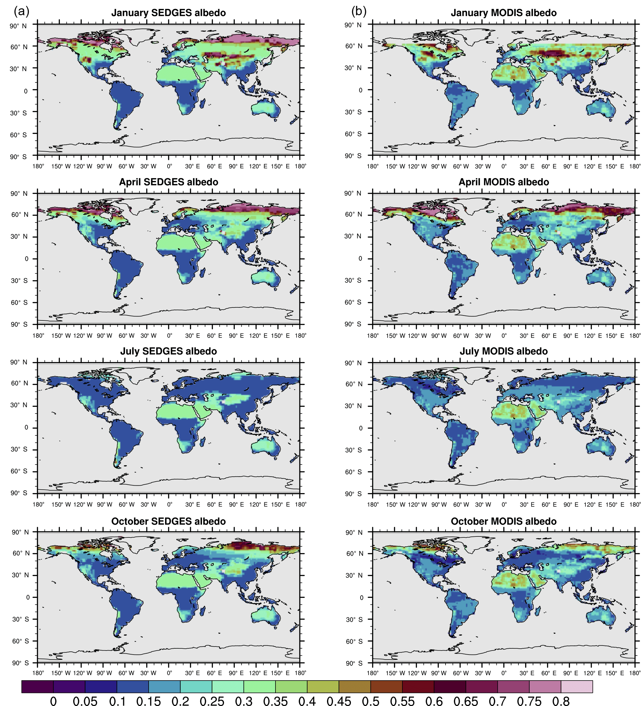
Figure 4 (a) SEDGES monthly mean climatologies of surface albedo for 2001–2010. (b) MODIS monthly mean climatologies of white-sky albedo for 2001–2010 (NASA LP DAAC, 2008b).

The soil albedo formulation in SEDGES is an advent to SimBA, which has always used a fixed soil albedo of 0.30. The new dynamic scheme was adopted, in part, due to the important role played by ground albedo in Sahelian/Saharan vegetation–precipitation feedbacks, as seen through its effect on low-frequency precipitation variability (Vamborg et al., 2014) and increased greening in the mid-Holocene (Vamborg et al., 2011). The new scheme also gives more realistic snow-free albedo values in the high latitudes and in the hot deserts (Fig. 4). While the above formulation for snow-free albedo, α₀, neglects, for simplicity, the radiative impact of non-photosynthesizing plant parts (e.g., stems and branches), this impact becomes important (although implicit) in the snow-covered formulation.

A new snow albedo scheme for SEDGES replaces the version from SimBA that linearly combines the albedos from the forested and flat portions of the grid cell according to the forest cover fraction. The SimBA formulation did not simulate well the sharp, real-world transition in snow-covered albedo from tundra to boreal forest (Loranty et al., 2014), which is why a new exponential decay scheme was developed.

In SEDGES, for snow depth > 0, the surface is treated as consisting of two components: (1) “flat” surface (consisting of exposed soil, prostrate vegetation, and dwarf shrubs) that can be partially or entirely buried by the snow cover; (2) “forest” that is covered by trees and shrubs of sufficient stature so as to protrude above the snowpack and mask it from the sun via their leaves, stems, and/or branches, regardless of accumulated snow depth on the ground. A nonlinear combination of the albedo of the flat portion and the snow-covered forest albedo yields the final surface albedo (α):

$$\begin{array}{}\text{(26)}& \mathit{\alpha }={\mathit{\alpha }}_{\mathrm{snow}\mathrm{for}}+({\mathit{\alpha }}_{\mathrm{snow}\mathrm{flat}}-{\mathit{\alpha }}_{\mathrm{snow}\mathrm{for}})e^{-c_{\mathrm{4}}\cdot max(\mathrm{0},{\mathrm{C}}_{\mathrm{veg}}-c_{\mathrm{5}})},\end{array}$$

where c₄ is a shape parameter, and c₅ is the biomass threshold (1.5 kg C m⁻²) at which the woody vegetation is sufficiently tall as to begin to mask the snow.

The albedo of the flat portion of the grid cell, α_snow flat, is formulated according to the same temperature dependency (Roeckner et al., 2003) and snow cover fraction (Roesch and Roeckner, 2006) schemes for non-forested areas in the ECHAM5 model, except that we maintain the melting snow albedo of 0.4 from PlaSim and ECHAM4 (Roesch et al., 2001) and we neglect the impact of sloping terrain. We thus have the following:

$$\begin{array}{}\text{(27)}& {\mathit{\alpha }}_{\mathrm{snow}\mathrm{flat}}={\mathit{\alpha }}_{\mathrm{0}}+({\mathit{\alpha }}_{\mathrm{deep}\mathrm{snow},\mathrm{flat}}-{\mathit{\alpha }}_{\mathrm{0}})\cdot \mathrm{0.95}{f}_{\mathrm{snow}\mathrm{flat}},\end{array}$$

where f_snow flat≡tanh(100 swe) is the fraction of the flat portion of the grid cell that is covered by snow (swe is the snow depth in liquid water equivalent (m³ m⁻²)),⁶ and α_{deep snow,flat} is the albedo of a deep and pure snowpack and is temperature dependent. This dependency has the form of a ramp function, with a maximum albedo, α_{max deep snow flat}≡0.8, for surface temperatures ≤ −5 ^∘C and a minimum albedo, α_{min deep snow flat}≡0.4, at melting point. These values are the same as in PlaSim and SimBA, except that they have maximum albedo attainment at −10 ^∘C.

The albedo of the forest component of the grid cell when there is snow cover is as follows:

$$\begin{array}{}\text{(28)}& {\mathit{\alpha }}_{\mathrm{snow}\mathrm{for}}\equiv min({\mathit{\alpha }}_{\mathrm{snow}\mathrm{flat}},{\mathit{\alpha }}_{\max \mathrm{snow}\mathrm{for}}).\end{array}$$

Here, α_{max snow for} is the maximum snow-covered albedo for forest and is set to 0.30, a midrange white-sky albedo value for the different forest types (Moody et al., 2007). Restricting α_snow for to not exceed α_snow flat is done because the lower snow depth and warmer snow that reduce the albedo of the flat area also lower the albedo of the forested area to at least the level of the flat area.

2.3.2 Soil bucket depth

We first introduced the soil bucket depth, W_max, in Sect. 2.2.5 in Eq. (12). SEDGES uses a simplified version of the parameterization in the JeDi (Jena Diversity) dynamic global vegetation model (Pavlick et al., 2013). The JeDi model uses a pipe representation of the rooting system (Shinozaki et al., 1964) in which a square root relationship emerges between W_max and coarse root biomass as a result of an assumed constant density of fine roots in the rooting zone. To adapt this formulation to SEDGES, we further assume that coarse root biomass is a fixed fraction of total biomass and that the unit plant-available water capacity is spatially constant. Doing so gives the following relationship:

$$\begin{array}{}\text{(29)}& W_{max}=min\left({W_{max}}_{min},c_{\mathrm{12}}\sqrt{{\mathrm{C}}_{\mathrm{veg}}}\right),\end{array}$$

where c₁₂ is a tuning parameter set to 0.10 kg C^1∕2. This value yields soil bucket depths that are a reasonably good fit with a plant-available water dataset based on optimal rooting depths (Kleidon and Heimann, 1998; Hall et al., 2006; Kleidon, 2011). In that dataset, the soil bucket depths in the most sparsely vegetated regions range from around 0.05 m in the Canadian polar desert to < 0.003 m in the hyperarid Atacama and northeast Sahara deserts. SEDGES adopts a minimum soil bucket depth, $W_{{max}_{min}}$, of 0.05 m.

The versions of SimBA (Kleidon, 2006b; Lunkeit et al., 2007, 2011) compute W_max using the following formulation: $W_{max}=Z\times W_{{max}_{max}}+(\mathrm{1}-Z)W_{{max}_{min}}$, where Z is the forest cover fraction formulation in the original SimBA (see Sect. 2.2.9) and $W_{{max}_{max}}$ is some maximum value for W_max. This W_max formulation was updated in SEDGES because the new formulation has the advantage of being derived from first principles (Pavlick et al., 2013).

2.3.3 Surface roughness

SEDGES has been designed for use in land surface schemes in which the surface roughness lengths for momentum and water vapor are the same (e.g., schemes that use parameterizations from Louis, 1979; Louis et al., 1982). As such, SEDGES returns only a single value for surface roughness length, z₀, for a grid cell. The (total) surface roughness is comprised of a surface roughness due to orography and a surface roughness due to vegetation:

$$\begin{array}{}\text{(30)}& z_{\mathrm{0}}=\sqrt{{z_{\mathrm{0}\text{veg}}}^{\mathrm{2}}+{z_{\mathrm{0}\text{oro}}}^{\mathrm{2}}},\end{array}$$

where z_0oro is the orographic surface roughness and z_0veg is the roughness due to vegetation. z_0oro is used by some GCMs (including Planet Simulator) to account for the enhancement of surface drag due to sub-grid-scale topographic variation (e.g., see Beljaars et al., 2004). z_0oro is set to 0 by default because small-scale orographic variation has little effect on land-to-atmosphere moisture transfer (Huntingford et al., 1998; Blyth, 1999).

In the SimBA formulation, surface roughness due to vegetation is parameterized assuming that only forest cover increases it appreciably and that prostrate vegetative cover does not. As such, sparsely vegetated surfaces are assigned too high of a surface roughness. SimBA has minimum and maximum values of z_0veg of 0.05 and 2 m, respectively (Kleidon, 2006b; Lunkeit et al., 2007, 2011). SEDGES replaces SimBA's linear dependency of z_0veg on forest cover fraction with the following logistic curve that depends on biomass rather than forest cover fraction:

$$\begin{array}{}\text{(31)}& z_{\mathrm{0}\text{veg}}={\displaystyle \frac{c_{\mathrm{17}}}{\mathrm{1}+e^{-c_{\mathrm{16}}({\mathrm{C}}_{\mathrm{veg}}-c_{\mathrm{15}})}}}-z_{\mathrm{0}\text{const}},\end{array}$$

where $z_{\mathrm{0}\text{const}}\equiv \frac{c_{\mathrm{17}}}{\mathrm{1}+e^{-c_{\mathrm{16}}(-c_{\mathrm{15}})}}-z_{\mathrm{0}\min }$ is a constant (in meters) that forces z_0veg to equal z_0min at zero biomass. The new formulation for z_0veg is tuned by adjusting c₁₅ and c₁₆ so as to roughly match reference values in the literature for different land cover types (especially those in Hagemann, 2002). z_0min is set to a bare-soil value of 0.01 m (Oke, 1987). c₁₇ represents the approximate maximum value of z_0veg and is assigned a value of 2.5 m, which is representative of tropical rain forests (Sellers et al., 1996b). z_0veg values that lie between these two extremes have been constrained by using the NPP–biomass relationship described in Sect. 2.2.9 and by visually comparing reference NPP and GPP values (Cramer et al., 1999; Jung et al., 2011), biome/land cover distribution maps (Ramankutty and Foley, 1999; Olson et al., 2001), and the aforementioned literature values of z_0veg for those land cover types.

3 How to couple SEDGES

As stated in Sect. 2.1, SEDGES is a DGVM and is to be embedded within a land surface scheme of a climate or Earth system model. As such, the input and output variables for SEDGES are not the same as those for the land surface scheme that SEDGES forms a part of because SEDGES has its own set of exchanges with the rest of the land surface scheme in which it lies.

At minimum, the following time-varying input fields are required by SEDGES: aerodynamic conductance (g_a), surface temperature (T_sfc), surface downwelling (broadband) shortwave radiation (SW↓), soil temperature at ≈ 0.20 m (T_soil), (bulk aerodynamic) potential evapotranspiration (PET), soil moisture content (W_soil), surface pressure (p_surf), and snow depth water equivalent (swe). Most of these variables are either calculated by or made accessible to fully fledged land surface schemes.

Other variables that are used by SEDGES will usually be part of the land surface scheme and depend on additional input variables (not listed in the previous paragraph). This is also the case when using ERA-Interim (ECMWF Reanalysis – Interim) data to force SEDGES (Sect. 4). In addition, the following parameter values (see Table 2) are not specified within the actual SEDGES code, which means that they must be declared and assigned values either in outside modules (e.g., in the non-SEDGES part of the land surface scheme) or by modifying the current SEDGES code: ϵ_max, atmospheric CO₂ concentration (c_a), the gas constant for dry air (R_d), maximum transpiration rate (trmax), and residence times for vegetative and soil organic carbon at 10 ^∘C (τ_veg and τ_soil).

SEDGES returns the following output fields: live vegetative biomass (C_veg), soil organic carbon (C_soil), soil water-holding capacity (W_max), surface wetness factor (C_w), transpiration (T) (as a diagnostic), evaporation from bare soil (only when snow is present), canopy resistance (r_c), minimum canopy resistance (r_cmin), surface albedo (α), total surface roughness (z₀), forest cover fraction (f_for), leaf area index (LAI), leaf cover fraction (f_leaf), net primary productivity (NPP), light-limited gross primary productivity (GPP_L), temperature limitation function (f₂(T_sfc)), water-limited gross primary productivity (GPP_W), litterfall (L), and soil respiration (R_soil).

In general, the land surface modeling framework that SEDGES presupposes must be reconciled with that of the land surface scheme of the Earth system or climate model that one is incorporating SEDGES into. In particular, in the absence of modification to either SEDGES or the original land surface scheme, the simulation of evapotranspiration according to the simplified mosaic and bulk aerodynamic formulations described in Sect. 2.1 and 2.2.5 is required. The requirement arises because the water and CO₂ exchanges predicted through this framework are presupposed by the canopy resistance equations. The simplest and recommended scenario with regards to reconciling soil hydrology is that the land surface scheme use a single-layer bucket model because this is what SEDGES “sees” when calculating soil surface and canopy resistances. As an example, Eq. (31), used in our forcing of SEDGES with ERA-Interim data (Sect. 4), gives the standard hydrological formulation for the simple single-layer bucket model.

In the likely scenario that the original land surface scheme of the Earth system or climate model does not perfectly match the framework used by SEDGES, it should, in many cases, be easy to achieve consistency of frameworks by adapting SEDGES and/or the original land surface scheme. Such adaptation would be easiest for the case in which the land surface scheme uses a single or multiple tile/mosaic approach because this approach could be converted to the simplified mosaic framework of SEDGES by, at each time step, replacing tile surface temperatures and soil wetness fractions with their respective grid-cell-weighted averages and by computing an effective surface roughness for the grid cell (e.g., Mason, 1988) in the case of significant areal water body coverage.

Finally, many land surface schemes distinguish between a surface roughness length of water vapor and heat from a surface roughness length of momentum, which is done to correct the typical bulk aerodynamic formulation for its replacement of temperature at the height of the roughness length with surface temperature (e.g., see discussion and references in Chen et al., 1997a). Although SEDGES only computes a roughness length of momentum, there are many ways to convert this roughness length to the roughness length for vapor/heat (e.g., see analyses and references in Chen et al., 2010).

An advantage of SEDGES is that (at least in principle) it can be run at any horizontal and temporal resolution. However, we encourage users to run the model using a sub-daily time step so that the generally positive diurnal covariances of light, temperature, aerodynamic conductance, and surface-to-air specific humidity difference can be adequately captured. These covariances should increase ET, overall. On the other hand, if users choose a daily time step or longer, then they should also anticipate an increase in vegetative productivity in water-limited regions due to the concomitant reduction in water stress. This reduction in water stress can be offset by decreasing trmax, the maximum transpiration parameter (Appendix Appendix B).

4 Forcing SEDGES with ERA-Interim data

In this section, we describe the process by which we force SEDGES using an external forcing dataset, with the goal of evaluating the capability of SEDGES as part of a land surface model. Repeated 1981–2010 6-hourly data from ERA-Interim (Dee et al., 2011) are used as the driver. The following required forcing variables (Sect. 3) were obtained from the reanalysis for direct input to SEDGES: surface (skin) temperature, surface downwelling shortwave radiation, temperature of the second-from-top soil layer, surface pressure, and snow depth water equivalent. Shortwave downwelling surface radiation is derived as follows: 3-hourly periods are isolated, and the two periods that straddle each given time (e.g., 12:00 Z straddled by the 09:00–12:00 Z and 12:00–15:00 Z periods) are averaged to give the flux at that time. A glacier mask is derived by considering any land point that has a daily mean snow depth always greater than zero to be glaciated. No vegetation occurs on glaciated grid points. Finally, all ERA-Interim data are interpolated to T62 resolution using climate data operators (CDOs) before being read into SEDGES.

In order to evaluate the performance of SEDGES, it is necessary to simulate soil hydrology in an interactive way rather than relying on soil moisture content from the external forcing dataset. (Early versions of SEDGES that were forced using reanalysis soil moisture resulted in unrealistic simulations of vegetation, especially in dry regions.) In order to do so, other land surface modeling components are combined with SEDGES, such that these components incorporate hydrologically relevant SEDGES output (namely, W_max, C_w, bare-soil evaporation (in the presence of snow), and z₀) and provide SEDGES with the variables needed: g_a, PET, and W_soil.

We simulate the aerodynamic conductance outside of SEDGES using these additional variables from ERA-Interim from the lowest atmospheric model level: the u and v wind components, the specific humidity, and temperature. The aerodynamic conductance and (bulk aerodynamic) PET are calculated according to the formulations of the Planet Simulator model (Lunkeit et al., 2011). Soil moisture content is simulated outside of SEDGES as a prognostic variable using a simple hydrological scheme and three additional ERA-Interim variables: precipitation, snowfall, and snowmelt. As we recommend above in Sect. 3, we use a single-layer bucket model, with bucket depth determined by SEDGES. The bucket model is simple. As such, runoff is from the surface and only occurs when the soil moisture content exceeds the bucket depth. Infiltration of liquid water from rainfall and from snowmelt is unrestricted. We use the discretized version of the following formulation to simulate soil moisture:

$$\begin{array}{}\text{(32)}& {\displaystyle \frac{\mathrm{\Delta }{W}_{\mathrm{soil}}}{\mathrm{\Delta }t}}=P-S+M-{\mathrm{ET}}_{\mathrm{soil}},\end{array}$$

where P is precipitation, S is the rate of snowfall, and M is the rate of snowmelt (all in liquid water equivalent). Again, W_soil cannot be greater than W_frac, with any excess going into runoff. Here, ET_soil is the combined soil evaporation and transpiration (and thus not coming from the snow cover). Recall from Sect. 2.2.5 that when there is snow cover, soil evaporation (E_soil) is calculated by SEDGES. Under conditions of sufficient snow cover (see below for more), transpiration is 0 and ET_soil reduces from being the (total) ET to being E_soil.

Soil hydrology in the framework we have constructed for driving SEDGES requires careful treatment in the presence of non-zero snow depths. Such care is especially needed because of the Tiled ECMWF Scheme for Surface Exchanges over Land (TESSEL) that is used by ERA-Interim and the data interpolation to the coarse T62 grid. The underlying TESSEL tile scheme and the spatial interpolation imply that data for a given grid cell that are fed into SEDGES can be physically inconsistent in the SEDGES framework (Sect. 2.1). The inconsistency arises because a grid cell can have a non-zero snow depth and yet have a homogeneous (as required and seen by SEDGES) surface temperature that is well above 0 ^∘C. This situation, in the absence of any modification to the SEDGES code, gives rise to common occurrences in which there is substantial transpiration from snow-covered leaves and in which snow-covered vegetation and ground are evaporating as if their surface temperatures were well above freezing. These occurrences are not only unphysical; they give rise to higher simulated ET from a given snowy, above-freezing region than would occur over the same region if it were divided up into its original small, homogeneous but differing tiles.

A second issue that must be addressed when there is snow is the tendency for ERA-Interim to overpredict freezing rain at the expense of snowfall (Dutra et al., 2011). Because we treat rain as entering the soil without interception by the snowpack (as is done in the TESSEL land surface model; Dutra et al., 2010), the freezing-rain bias led our early simulations to have an unrealistically large recharge of soil water reservoirs in winter in many locations, even though surface temperatures were well below 0 ^∘C. The handling of the aforementioned snow-temperature inconsistency and the freezing-rain bias are discussed next.

In order to simply resolve the above issue of snow with above-freezing temperature, we separate possible conditions into two cases: (1) swe > snow thresh and (2) swe ≤ snow thresh, where we define snow thresh as the swe threshold above which the surface is treated as snow-covered with respect to evaporation from and the physiology of vegetation and the threshold at or below which the surface is treated as snow-free. In case 1, we assume that transpiration is negligible (due to combined cold temperature and physical coverage of leaves by snow) and thus introduce a slight modification to Eq. (2), by setting f₂(T_sfc) to 0 (its value at freezing), which, in turn, forces the productivity to 0. In case 2, we assume that evaporation from snow is negligible, and f₂(T_sfc) is as normal. Finally, we address the excessive partitioning of precipitation into liquid form at subfreezing temperatures by further assuming for case 1 that soil moisture cannot increase unless there is some snowmelt during the same time step. Snowmelt indicates the presence of above-freezing temperatures and, thus, the presence of liquid water that does not freeze on contact with the surface and can thus infiltrate into the soil.

5 Model evaluation

In this section we evaluate SEDGES as part of the simple hydrological scheme described in Sect. 4, forced with ERA-Interim data. We emphasize the results from the simulation forced with historical CO₂, using reference datasets of vegetative carbon, LAI, surface albedo, tree cover fraction, soil organic carbon, GPP, and evapotranspiration.

Four simulations are carried out: three equilibrium simulations and one transient simulation. In the three equilibrium simulations, atmospheric CO₂ levels of 280, 360, and 560 ppm are held fixed through the simulations. The vegetation is spun up from a vegetative and soil organic carbon-free state. The spin-up includes an acceleration of the carbon cycle for the first 260 years (only). From simulation year 261 to year 1500, the carbon cycle is run normally. The model is very nearly at equilibrium by the last 30 years in all three runs, and these years are thus analyzed. The transient simulation begins with the end state of the 280 ppm equilibrium simulation and is subsequently forced using observed, transient atmospheric CO₂ values from 1832 to 2010. The CO₂ data are taken from the Mauna Loa dataset (Keeling et al., 1976) for 1959 and onward and from 20-year smoothed ice core data (Etheridge et al., 1998) for the prior years. Unless stated explicitly, the results and analyses always refer to the transient CO₂ simulation. The model performs reasonably well, overall; GPP is simulated exceptionally well. In the evaluation process, we concentrate on the comparison of SEDGES with observation-based data products, but we sometimes supplement these comparisons with comparisons to land surface models and their performances, especially to the ENTS model (Williamson et al., 2006) because it is of similar complexity to SEDGES.

5.1 Evaluation of productivity

GPP that is simulated by reanalysis-forced SEDGES is evaluated against two observation-based datasets: the Multi-Tree Ensemble (MTE) (Jung et al., 2011) and CARBONES (CARBON fluxES and pools over Europe and the globe; http://www.carbones.eu/wcmqs/project/). In addition, we use the model intercomparisons of Sitch et al. (2008), Piao et al. (2013), and Anav et al. (2015) and modeling-based results of Hemming et al. (2013) and Holden et al. (2013) to assess the relative performance of SEDGES.

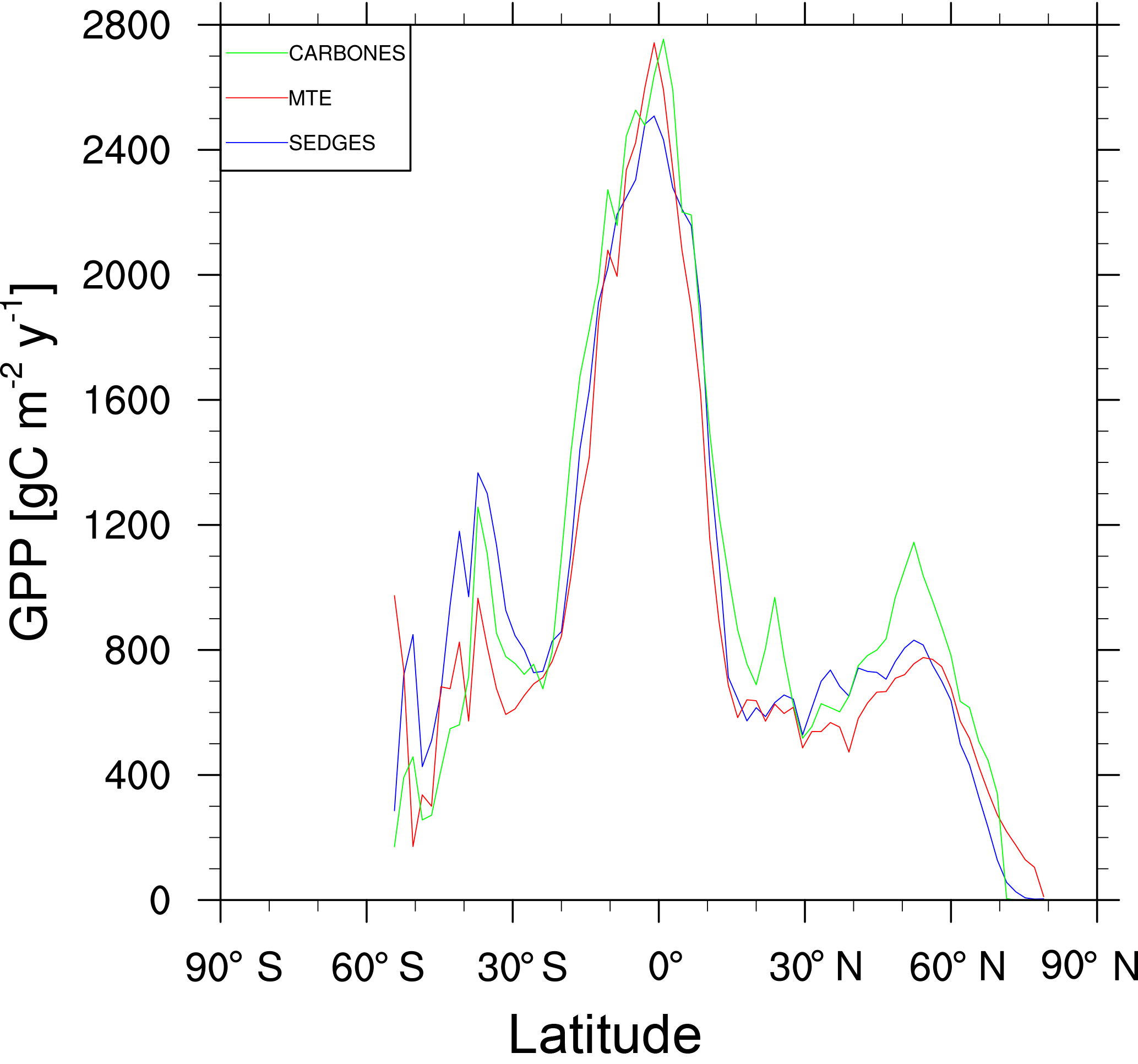
Figure 5 Zonal multiyear annual mean of GPP for SEDGES and the two reference datasets, MTE and CARBONES, for 1990–2009 over non-glaciated land.

Mueller et al. (2013)(Jung et al., 2011)Olson et al. (1985)(Wieder et al., 2011)

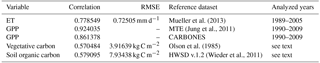
Table 3 RMSEs and correlations between multiyear annual means of SEDGES variables and those for reference datasets

For the 1982–2008 period, SEDGES simulates a global mean annual GPP of 126 Pg C yr⁻¹ as compared to 120 Pg C yr⁻¹ for the observation-based MTE dataset (Jung et al., 2011). Zonal means of GPP, taken over the glacier-free land mask obtained from the ERA-Interim data and for 1990–2009, are shown for SEDGES, MTE, and the CARBONES data assimilation dataset in Fig. 5. SEDGES captures the large-scale patterns very well. Compared to the two reference datasets, SEDGES has positive productivity biases in most of the Southern Hemisphere and around 35^∘ N, and it has negative biases near the equator and in the high northern latitudes. Moving to the full spatial field, we can see in Fig. 6 that the annual mean GPP, for 1990–2009, in SEDGES and MTE compares very well, overall, with those of MTE and CARBONES. Regionally, as compared to the two reference datasets, SEDGES simulates too high a GPP in western Argentina, in nondesertic tropical Africa, around the Korean Peninsula, and on the southwestern and eastern Australian coasts and too little GPP in almost all the equatorial tropics and Amazonia (see Sect. 5.6 for discussion), the Pacific northwest of the United States, northwestern Europe, and parts of north-central and far eastern Siberia. In Siberia, SEDGES simulates too low a GPP in a dry region northeast of the Kolyma Mountains. This underestimate may be partially due to SEDGES's neglect of leaf mitochondrial respiration in the light, which has been found to be a large fraction (up to ≈ 0.3) of gross photosynthesis in Arctic tundra plants (McLaughlin et al., 2014; Heskel et al., 2014). Indeed, a fraction of 0.3 would, under purely water-limited conditions, increase GPP by 43 %.

The spatial correlations between SEDGES and the reference datasets are as high as can be expected (Table 3). Spatial correlations between multiyear annual means of GPP from MTE and three offline land surface models (ORCHIDEE, ORganizing Carbon and Hydrology in Dynamic EcosystEms (Krinner et al., 2005); JULES; and CLM4CN, Community Land Model with coupled Carbon and Nitrogen cycles, Lee et al., 2013) range from ≈ 0.87 to 0.95 (Anav et al., 2015), whereas it is 0.92 for SEDGES. The same correlations between the three models and CARBONES ranges from ≈ 0.83 to 0.87 (Anav et al., 2015), whereas it is 0.86 for SEDGES.

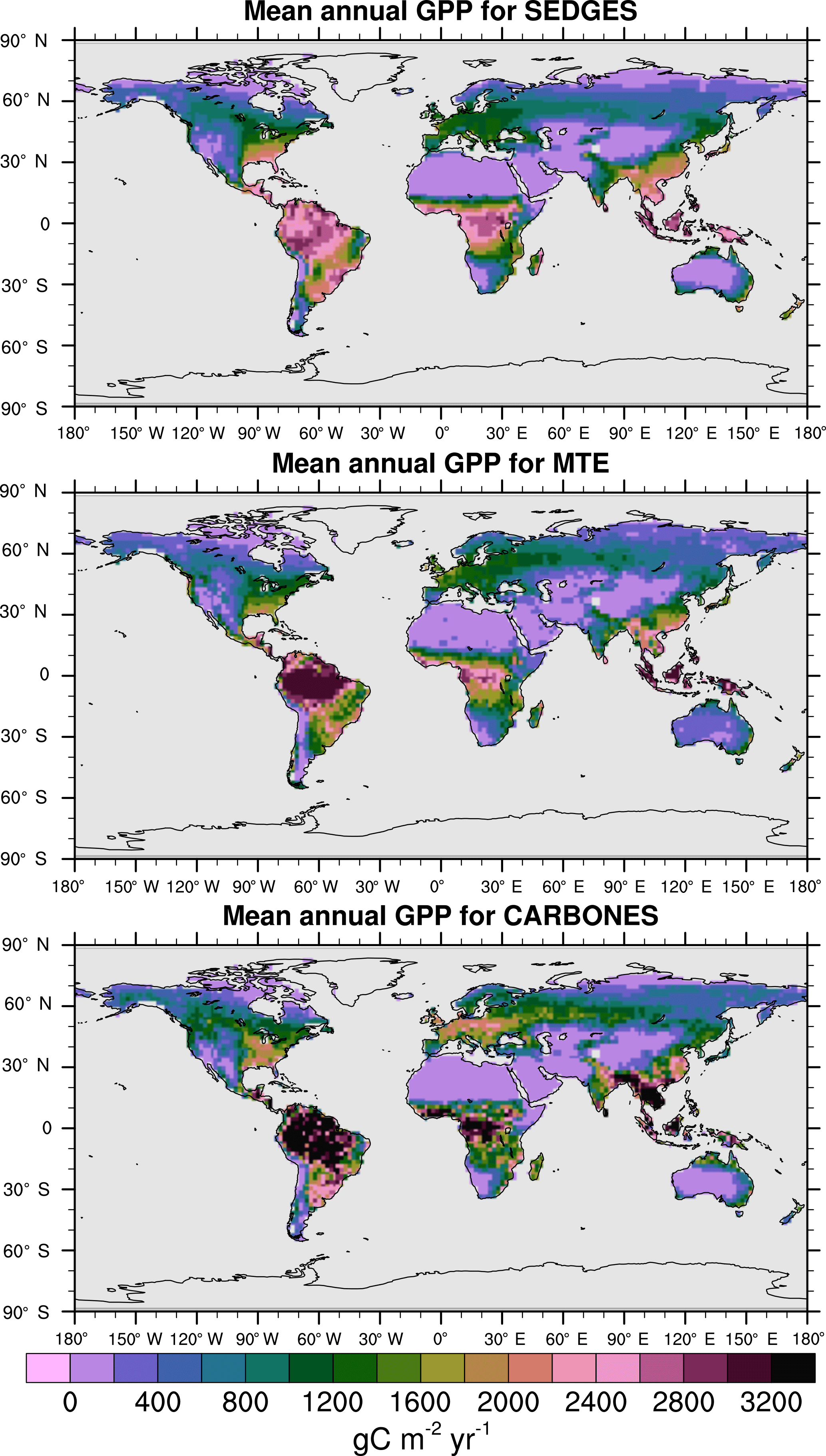
Figure 6 Multiyear annual mean of GPP for SEDGES and the two reference datasets, MTE and CARBONES, for 1990–2009 over non-glaciated land.

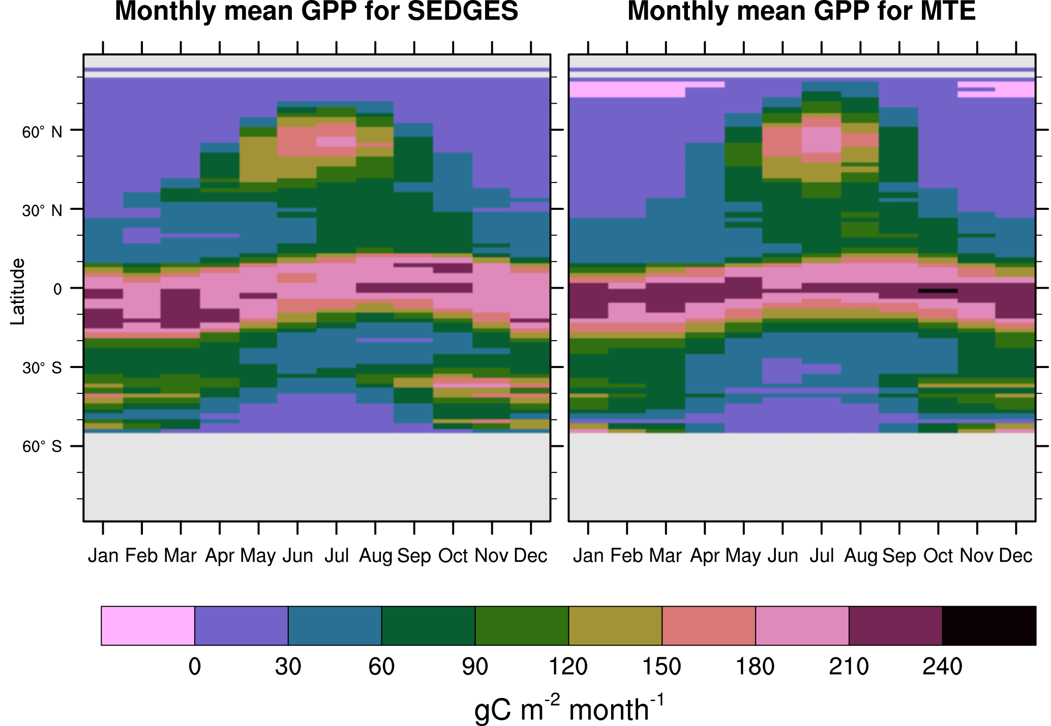
Figure 7 Zonal multiyear monthly means of GPP for SEDGES and the MTE reference dataset for 1982–2010 over non-glaciated land.

SEDGES simulates the multiyear monthly means of GPP well, as shown by comparison with those for the MTE dataset in Fig. 7 for different latitudinal bands. From this figure, we can see that SEDGES captures the seasonal progressions of GPP well. A noticeable departure of SEDGES from MTE, however, is a slight phase shift in the Northern Hemisphere extratropics, with a generally earlier spring productivity increase in SEDGES than in MTE. We suspect that the phase shift is due to the absence of both winter-deciduous leaf phenology and physiological constraints on the speed of acclimation to temperature (discussed more in Appendix Appendix A). Moving to the full spatial field, Fig. 8 shows that the correlations in the seasonal cycle between SEDGES and MTE are generally high in areas with a strong seasonality of productivity such as the mid- to high latitudes, India, and the dry tropics. Temporal correlations are weaker, but still generally positive, in semiarid regions and in Amazonia. Correlations are often negative in regions with low absolute seasonal variation in GPP such as equatorial Africa, the northern hemispheric deserts, and southern Australia. SEDGES's problems in the dry regions may be due to the simple single-layer bucket soil hydrology that was used. The negative correlation in equatorial Africa is due to insufficient moisture stress in that region in ERA-Interim-forced SEDGES. The lack of moisture stress in this region causes dry-season GPP to exceed that of the wet season due to the reduced cloud cover, as is seen in the wetter parts of the Amazon (Wu et al., 2016). However, the real African equatorial forest experiences a drop in GPP during the dry season relative to the wet season (Guan et al., 2015). Thus, the real-world behavior in equatorial Africa is anticorrelated with that in the model. In equatorial Africa, the lack of moisture stress in ERA-Interim-forced SEDGES is likely attributable to a pronounced positive precipitation bias in the ERA-Interim forcing data in that region (Lorenz and Kunstmann, 2012; Dolinar et al., 2016).

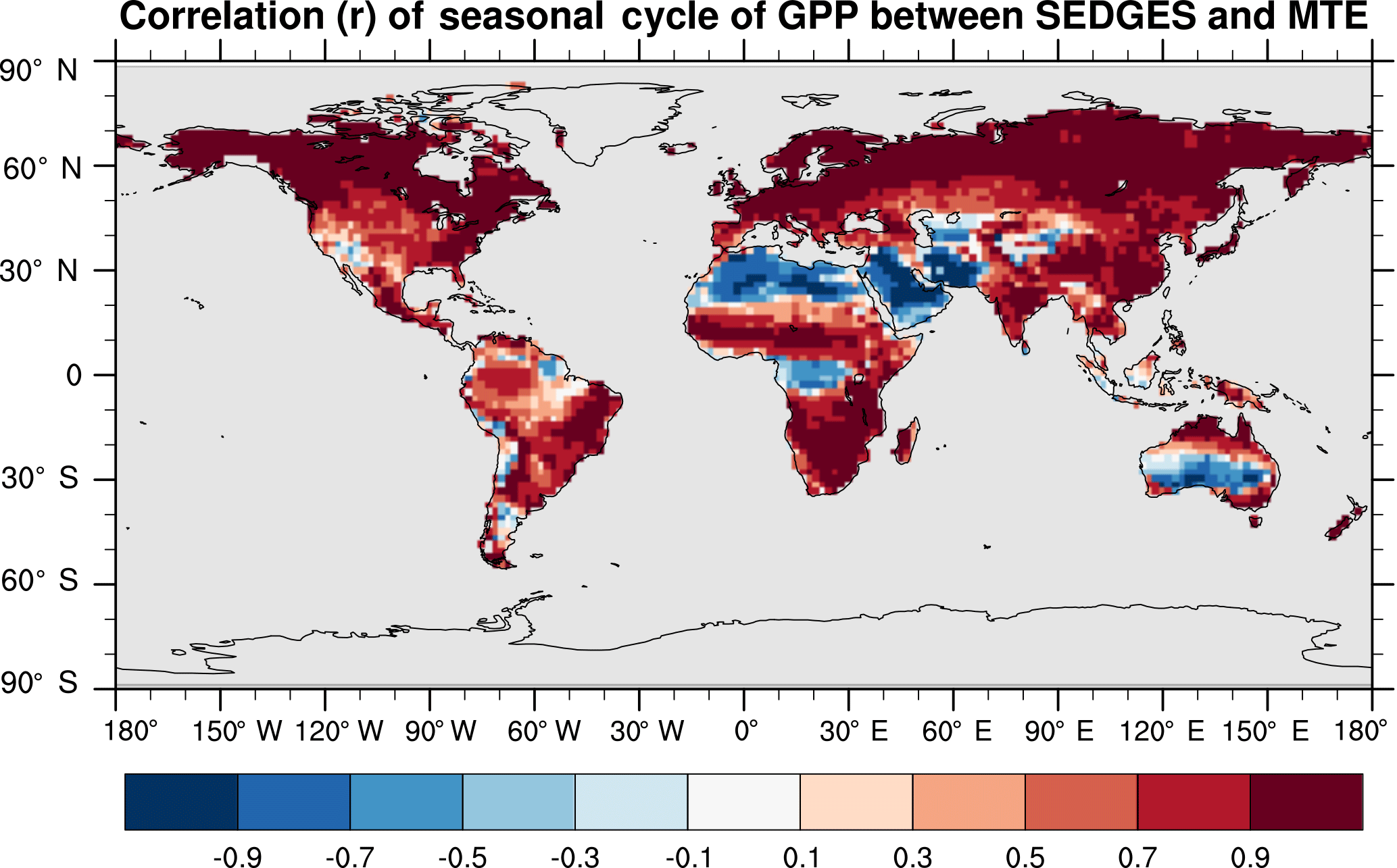
Figure 8 Pearson correlation coefficients of the seasonal cycle (i.e., of the multiyear monthly means) between SEDGES and the MTE reference dataset for the 1986–2005 period.

The interannual variability in global GPP for 1990–2009 in SEDGES is 1.79 Pg C yr⁻¹, whereas it is 2.50 Pg C yr⁻¹ for the CARBONES dataset. Anav et al. (2015) report values of 3.23, 4.4, and 2.87 Pg C yr⁻¹ for the offline-driven land surface models ORCHIDEE, JULES, and CLM4CN, respectively. The interannual variability in GPP at each grid point is shown in Fig. 9 for SEDGES and CARBONES. SEDGES successfully captures the spatial pattern of the CARBONES reference dataset, although its magnitudes are smaller, overall. These smaller magnitudes are probably attributable to a number of factors. Figure 9 shows that SEDGES most severely underestimates interannual GPP variability in cropland regions (cf. Ramankutty et al., 2008), which can differ greatly in form and function from the natural vegetation simulated by SEDGES. Secondly, the underestimate of mean annual GPP by SEDGES in some regions such as northern Asia (Fig. 6) likely contributes to the model's underestimate of GPP variability in those same regions. Finally, SEDGES applies the same temperature limitation function to productivity (Appendix Appendix A) in all situations. In so doing, the model underestimates physiological constraints on the speed with which vegetation can adapt to new thermal regimes. Although in real life these constraints apply mostly on daily timescales, interannual variation in the frequency of extreme temperature events probably has greater impact on annual GPP in the real world than in SEDGES.

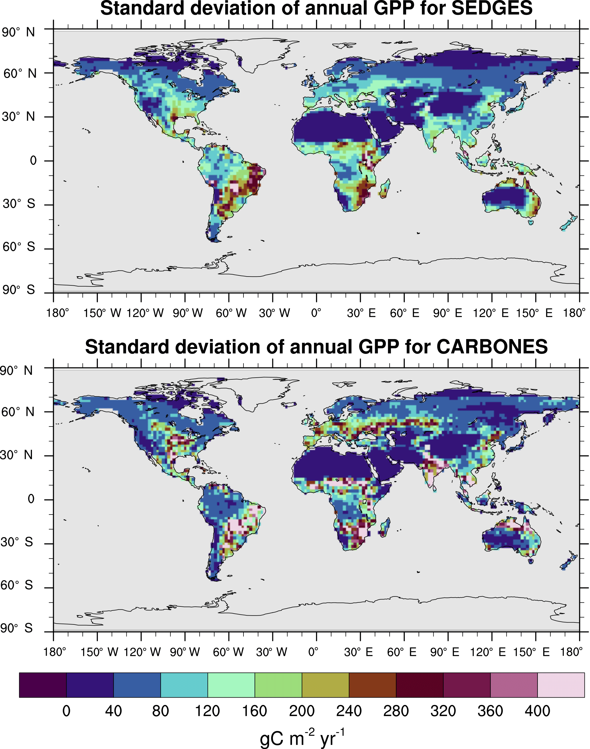
Figure 9 Interannual variability in GPP for SEDGES and the CARBONES reference dataset for the 1990–2009 period.

The trend in annual GPP for 1990–2009 is captured extremely well by SEDGES. The CARBONES reference dataset yields a global annual GPP trend of 0.086 Pg C yr⁻², whereas SEDGES gives a value of 0.080 Pg C yr⁻². The spatial pattern of the trend is seen in Fig. 10. SEDGES captures the spatial pattern of GPP trend in the CARBONES dataset better than ORCHIDEE, JULES, and CLM4CN, as reported by Anav et al. (2015). SEDGES generally outperforms the other models in Africa, Australia, the semiarid areas of eastern Europe, and central and eastern Asia. Notable areas where SEDGES (but not the other models) deviates from CARBONES include the Amazon and parts of northwestern North American, in which SEDGES simulates more negative trends in GPP than the reference dataset. The negative GPP trend in SEDGES in the Amazon is very possibly due, at least in part, to its simplifications affecting the CO₂ fertilization of productivity, as is explained next.

The SEDGES treatment of CO₂ fertilization is seen via Eqs. (3) and (6) and notably lacks a direct dependency on temperature. However, Long (1991), using the widely used Farquhar model of photosynthesis (Farquhar et al., 1980), finds that, for a given $\frac{c_{\mathrm{i}}}{c_{\mathrm{a}}}$, the proportional increase in leaf photosynthesis with elevated CO₂ increases substantially with temperature under both Rubisco- and light-limited conditions. In line with that result, a modeling study on the scale of a global grid (Hickler et al., 2008) which uses a photosynthesis model based on that of Farquhar, finds that the fertilization response of NPP to elevated CO₂ increases substantially, too, when moving from boreal forest to temperate forest to tropical forest. Hence, if SEDGES were to use a more complex parameterization of photosynthesis that is based on the Farquhar model, one would expect the Amazon region to show a more positive GPP trend in Fig. 10 and thus be closer to the CARBONES data.

In spite of the simplifications affecting CO₂ fertilization in SEDGES, its global productivity response to CO₂ forcing is comparable to that of other models of the land surface and vegetation. The results of transient experiments in which 10 such models are forced offline with repeated early 20th century climate and with increasing CO₂ values show relative increases in global NPP per ppm CO₂ of 0.05 to 0.20 % (with mean of 0.16 %) for the 1980–2009 period (Piao et al., 2013); it is 0.102 % for SEDGES. Similar transient simulations with five of the aforementioned models (but also including projected CO₂ levels) (Sitch et al., 2008) give global GPP increases⁷ from 280 to 360 ppm CO₂ that range from approximately 14 to 19 %; they give global GPP increases from 360 to 560 ppm CO₂ that range from approximately 23 to 36 %. In comparison, the transient run of SEDGES gives an increase in global GPP from 280 to 360 ppm CO₂ of 20 % and an at-equilibrium global GPP increase from 360 to 560 ppm CO₂ of 30 %. Finally, Hemming et al. (2013), approximating the purely physiological effect⁸ of CO₂ on productivity using a GCM, finds an increase in equilibrium GPP of 75 % when doubling CO₂ from near-preindustrial values. A most likely increase in global NPP of 40 to 60 % with CO₂ doubling from preindustrial levels is found by Holden et al. (2013), using a combination of global atmospheric CO₂ rise and estimated land use changes since the preindustrial period. Doubling preindustrial CO₂ (280 to 560 ppm) in equilibrium simulations in SEDGES induces an NPP increase of 55 %.

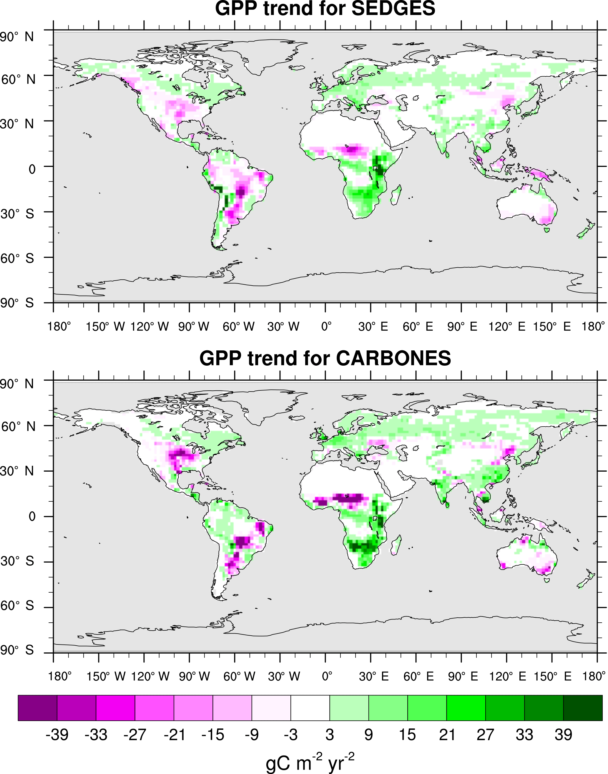
Figure 10 Linear regression trend in annual GPP for SEDGES and the CARBONES reference dataset for 1990–2009.

5.2 Evaluation of vegetative carbon

Vegetative carbon is simulated reasonably well by SEDGES. Unless stated otherwise, we compare the means of the last 30 years of the CO₂-varying run with an older reference dataset (Olson et al., 1985). The Olson dataset was chosen because its data sources reflect the potential natural vegetation better than the sources of the more recent NDP-017b (NDP – numeric data package) dataset (Gibbs, 2006). SEDGES has an equilibrium global vegetative carbon of 530 Pg C under preindustrial levels of CO₂ and a mean of 615 Pg C for 1981–2010 of the transient CO₂ run. In comparison, the Olson et al. (1985) dataset and the more recent Gibbs (2006) dataset give global vegetative carbon of 451 and 560 Pg C, respectively (Jiang et al., 2015, citing Gibbs, 2006).

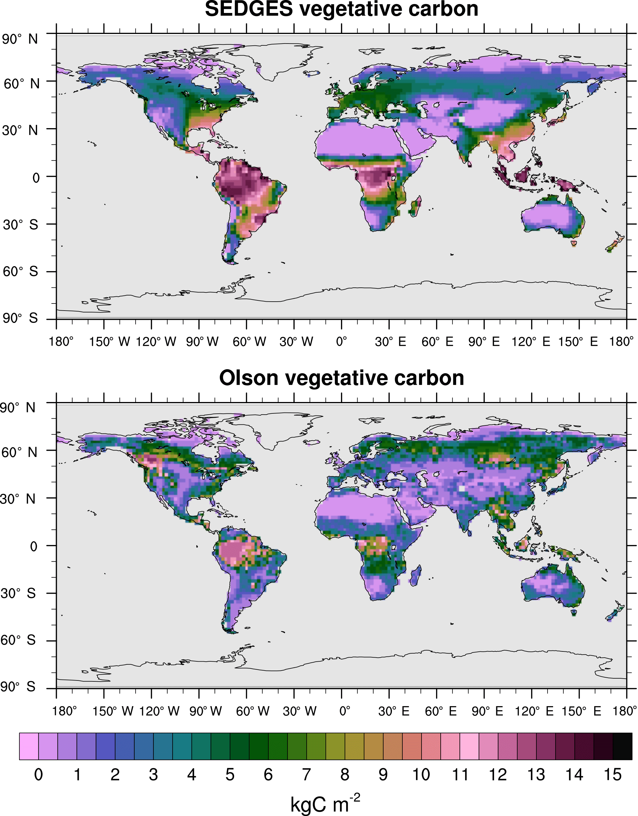
Figure 11 Vegetative carbon for SEDGES: mean over 1981–2010 in the transient CO₂ simulation; vegetative carbon from the Olson et al. (1985) reference dataset, which represents pre-Iron Age vegetation save for the most extreme anthropogenic land cover changes.

Figure 11 shows the distributions of mean vegetative carbon for SEDGES (1981–2010) and that for the Olson et al. (1985) dataset. The spatial pattern of Olson vegetative carbon is captured well by SEDGES (Table 3: R=0.57, R²=0.33). The RMSE (root mean squared error) between SEDGES and the Olson datasets is 3.92 kg C m⁻². (We calculate RMSE in this study by taking the square root of an area-weighted mean of the squared differences between SEDGES and the reference at each grid point.) Among the discrepancies, two tendencies prevail: the almost-direct relationship between GPP biases and vegetative carbon biases and an overall tendency to overestimate vegetative carbon in the tropics and to underestimate it in the mid- to high latitudes. SEDGES has large positive vegetative carbon biases in most of the tropics (except the western Amazon), southeast North America, China, and northwestern Europe. One should note that many of these biases reflect land cover change from forests to croplands (Ramankutty and Foley, 1999). In addition, positive biases in the wet-and-dry and semiarid tropics are partially attributable to the absence of a fire module in SEDGES; fire can have a large impact on vegetative cover in these regions (Bond et al., 2005). SEDGES has large negative biases in western Canada and central Siberia. The subarctic is generally negatively biased. These vegetative carbon biases are due to a combination of the aforementioned GPP biases and the globally uniform residence time for vegetative carbon in SEDGES (Table 2). The SEDGES 10-year residence time for vegetative carbon matches the observation-based estimate $\left(\equiv \frac{{\mathrm{C}}_{\mathrm{veg}}}{\mathrm{NPP}}\right)$ given by Jiang et al. (2015).

Compared to SEDGES, ENTS (Williamson et al., 2006) simulates vegetative carbon slightly closer to the Olson reference, overall. ENTS has a strong negative biomass bias in eastern Australia, and it greatly overpredicts biomass in eastern Brazil and northeastern Canada; SEDGES predicts these regions fairly well. On the other hand, ENTS also predicts more biomass in central Siberia (i.e., has a weaker negative bias), simulates western Canada well, has a less severe negative biomass in far eastern Siberia and Alaska, and has a less severe positive biomass bias in the tropics.

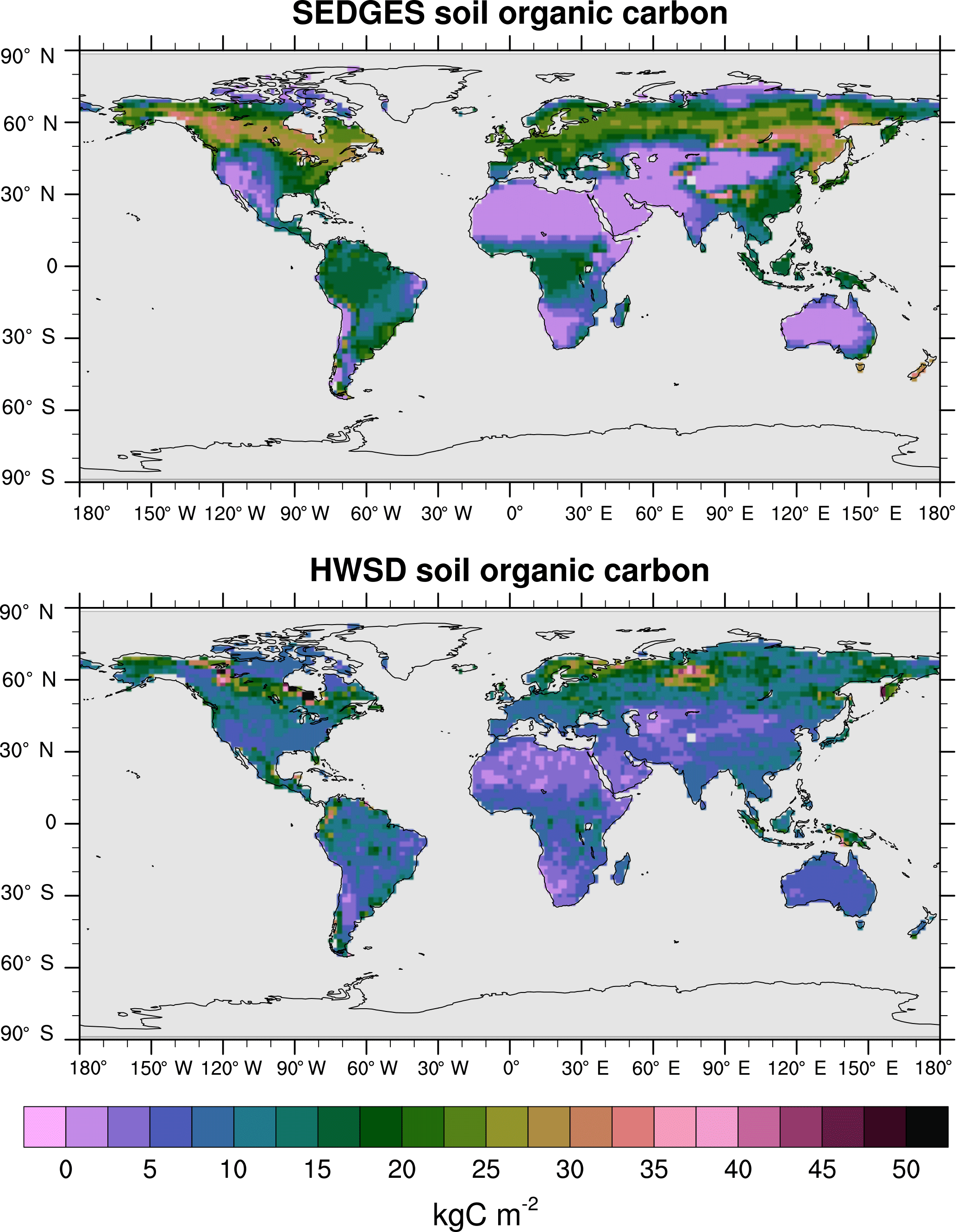
Figure 12 Soil organic carbon for SEDGES: mean over 1981–2010 of the transient CO₂ simulation; soil organic carbon from the HWSD reference dataset (Wieder et al., 2011). The HWSD dataset has values for the top meter of the profile, only.

5.3 Evaluation of soil organic carbon

At present, land surface models have great difficulty in simulating soil organic carbon well. Tian et al. (2015), using 10 offline-forced terrestrial biosphere models at 0.5^∘ resolution, find highly diverging model estimates of soil organic carbon dynamics as well as systematic biases due to absent processes affecting high-latitude soil organic carbon stocks. The models in Tian et al. (2015) have Pearson correlation coefficients under 0.4 with respect to the Harmonized World Soil Database (HWSD) reference dataset (Wieder et al., 2011). SEDGES performs better with a 0.58 correlation (at the coarser T62 resolution), although it should be kept in mind that model performance in simulating soil organic carbon has been found to improve dramatically when aggregating on large spatial scales (Todd-Brown et al., 2013). As listed in Table 3, SEDGES has a 7.9 kg C m⁻² RMSE with respect to the HWSD data.

Figure 12 shows the full spatial distribution of soil organic carbon for SEDGES and the HWSD reference dataset. Compared to HWSD, SEDGES simulates less soil organic carbon in semiarid and arid areas, in the more northern parts of the Arctic, and generally more soil organic carbon in the remaining areas. Compared to the ENTS model (Williamson et al., 2006), SEDGES gives a broadly similar simulation of soil organic carbon, as expected since their soil respiration formulations are almost identical. Some notable differences between the two are that SEDGES generally simulates more soil organic carbon than ENTS; SEDGES predicts too much soil organic carbon in southeastern North America, southeastern Asia, and the tropics, whereas ENTS generally does not; in high northern latitudes, ENTS (only) simulates a pattern of very high values in far eastern Siberia, Alaska/Yukon, and northeastern Canada with lower values in between, but this pattern is not seen in the HWSD dataset.

Taking the globe as a whole, SEDGES has a residence time for soil organic carbon of 25.7 years and a time-averaged soil organic carbon of 1516 Pg C for 1981–2010. Respective estimates for these values based on HWSD data are 24 years for residence time (Todd-Brown et al., 2013) and range from 891 to 1657 Pg C for total terrestrial soil organic carbon storage (Tian et al., 2015). Köchy et al. (2015) estimate total terrestrial soil organic carbon at a higher value of ≈ 3000 Pg C because they include estimates of carbon in the deeper soil layers that HWSD does not.

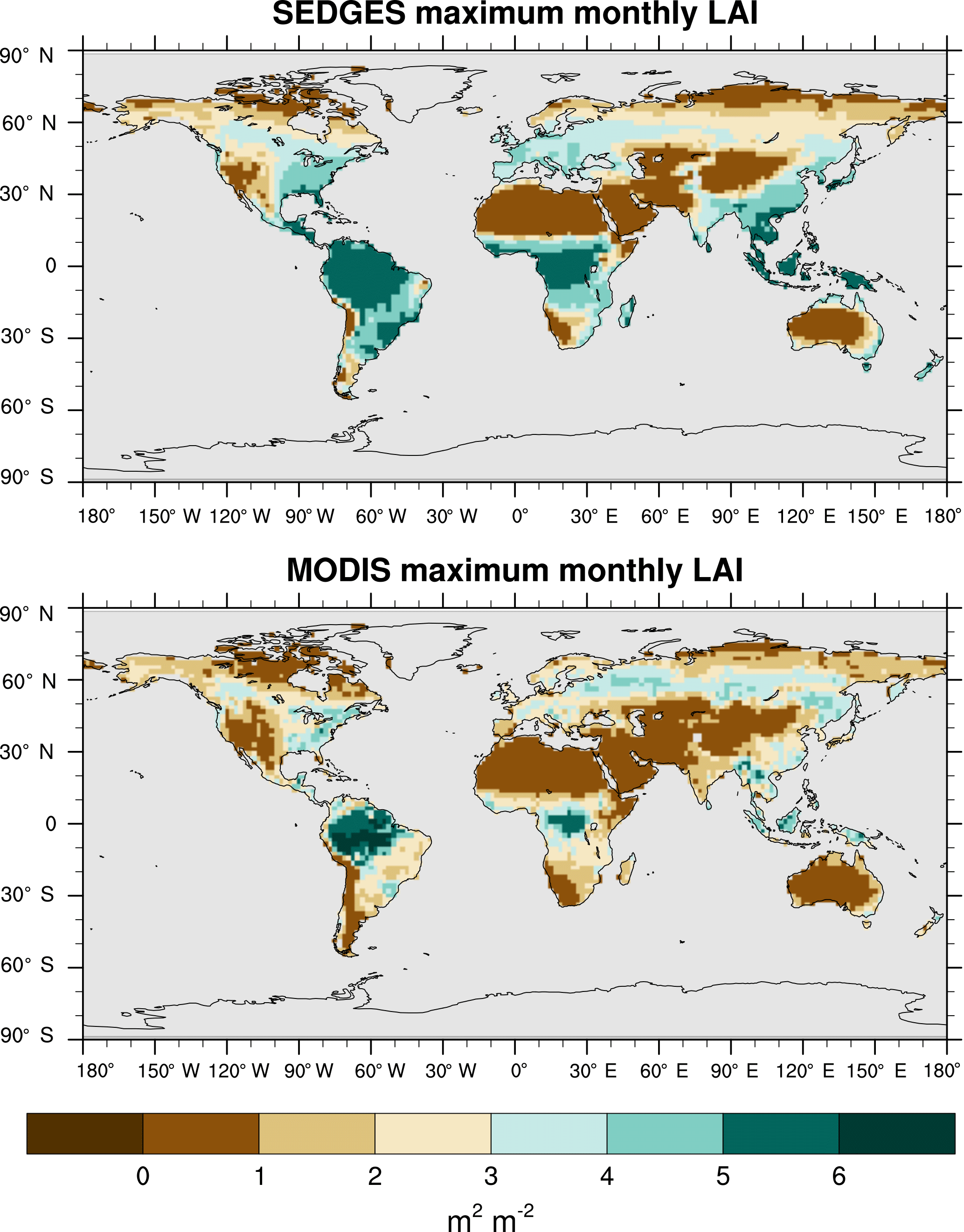
Figure 13 Maximum LAI of the multiyear monthly means for SEDGES and for the BNU MODIS-based reference dataset for the 2001–2010 period.

5.4 Evaluation of LAI

We use reprocessed Moderate Resolution Imaging Spectroradiometer (MODIS) data from 2001 to 2010 from Bejing Normal University (BNU) (Yuan et al., 2011) as the reference set. We interpolated these data to T62 resolution and derived multiyear monthly means from them. Outside of the tropics, we compare only the maximum of the multiyear monthly means of LAI between SEDGES and the reference data because of the absence of cold deciduous phenology in SEDGES and because serious deficiencies with MODIS in capturing the seasonal cycle of LAI in boreal coniferous forests have been found (Serbin et al., 2013).

Figure 13 shows the maximum multiyear monthly mean LAI in SEDGES and the BNU MODIS-based reference for the years 2001 to 2010. SEDGES has strong positive biases in southeastern and extreme northern South America, in parts of Africa, in parts of southern and eastern Asia, in northern coastal Australia, and in parts of Europe. Many of these LAI biases lie where positive GPP biases occur and/or where croplands have replaced natural forests. Strong negative biases occur in parts of northern Asia. Of these, the biases east and northeast of Lake Baikal occur in the absence of negative GPP biases. Overall, the spatial patterns of maximum LAI in SEDGES and the MODIS-based reference have a correlation of 0.793.

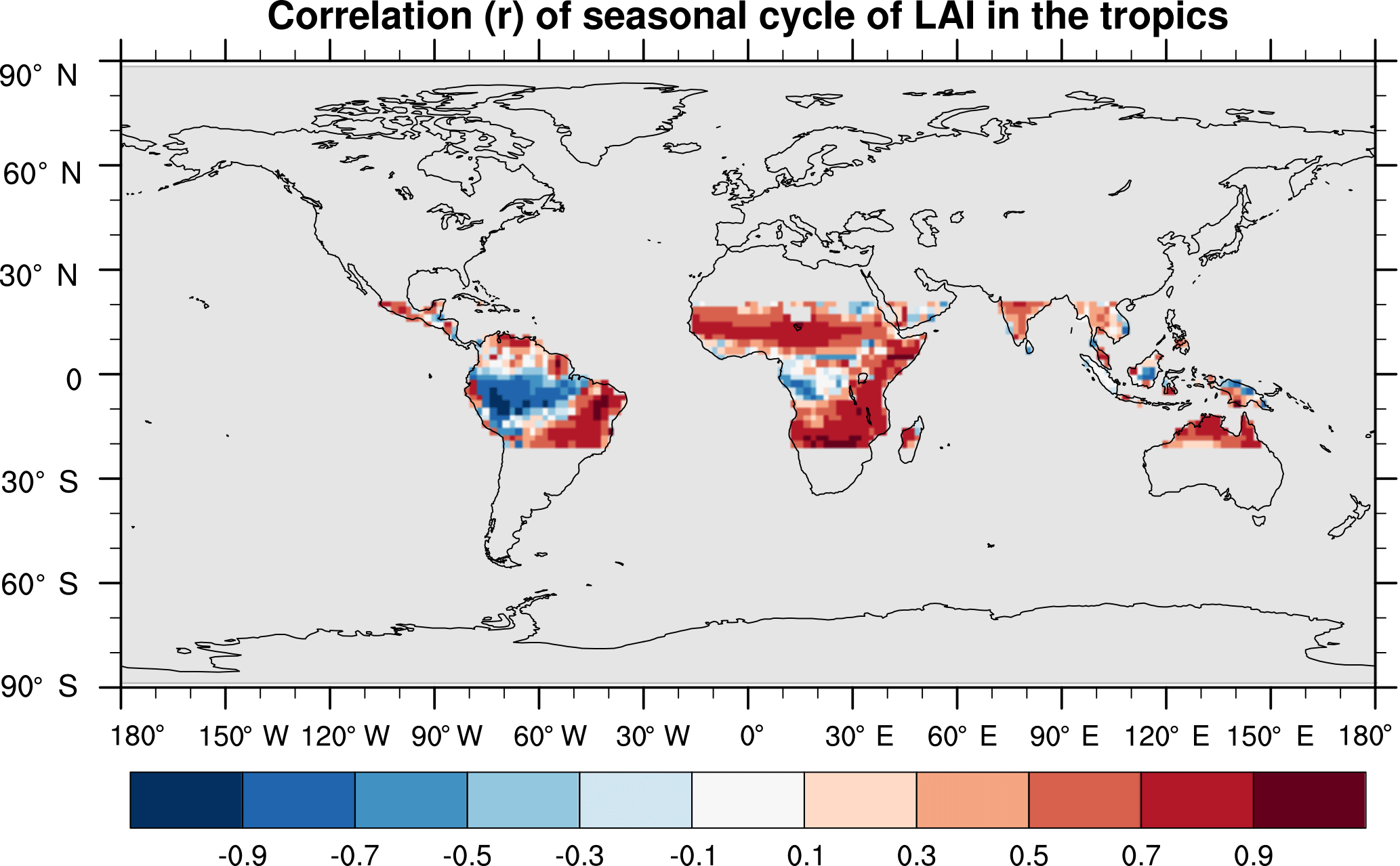
Figure 14 Temporal correlation at each grid point in the tropics (−20 to 20^∘) between the multiyear monthly means of LAI for 2001–2010 of SEDGES and of the BNU MODIS-based reference dataset. Some desert grid points do not have values because they have LAIs of 0 in one or both sets of data for all 12 months.

Figure 14 shows the temporal correlation in the tropics between the multiyear monthly means of SEDGES and the BNU MODIS-based reference (i.e., the correlations of the two seasonal cycles). In spite of the crude scheme for drought-deciduous phenology described in Sect. 2.2.8, SEDGES does a reasonable job in simulating the seasonal cycle of LAI in much of the tropics. Negative correlations (indicative of poor model performance) occur near the equator, especially in the Amazon region, where LAI varies modestly, seasonally, in the real world (e.g., Wu et al., 2016). The wet parts of the Amazon generally experience high water availability, even in the dry season. As a result, LAI there is decoupled from soil-moisture-induced water stress (in contrast with the drier portions of the Amazon) and LAI, generally, increases during the dry season and decreases during the wet season (Wu et al., 2016). SEDGES cannot capture this behavior.

5.5 Evaluation of surface albedo

Figure 4 shows monthly mean climatologies of SEDGES surface albedo and MODIS white-sky albedo (NASA LP DAAC, 2008b)⁹ for the months of January, April, July, and October for the years 2001 to 2010. From these figures, we can see that SEDGES captures the overall spatial albedo pattern fairly well. In fact, spatial correlations between SEDGES and the reference range from a low of 0.77 in July and August to a high of 0.91 in April. The high correlation in boreal spring indicates relative strength in simulating the winter melt season at mid- to high northern latitudes. The relative weakness of SEDGES in Northern Hemispheric summer is due to the absence of a strong snow signature on the land and relative weakness of the model in correctly capturing the second- and third-order determinants of (non-glacier) terrestrial albedo, since these determinants come to the fore during boreal summer. Three such determinants are now discussed.

The most significant model deficiency in albedo simulation that gains prominence during boreal summer is the simulation of bare-soil surface albedos. Recall from Sect. 2.3.1 that bare surface albedo in SEDGES is determined by soil organic carbon content and by the albedo of soil in the absence of soil organic carbon (α_sand), which is assumed constant. In the real world, geological processes, the quantity and properties of dead biomass litter, and the albedo of the underlying bedrock greatly impact α_sand as well (Knorr and Schnitzler, 2006; Vamborg et al., 2011). The absence of these real-world processes in SEDGES gives rise to an underestimate of albedo in the Arabian and the Saharan deserts and an overestimate of albedo in the snow-free season in most of the world's remaining deserts (Fig. 4). MODIS values of snow-free albedo (NASA LP DAAC, 2008a) in the polar desert (not shown) vary generally from 0.12 to 0.22 in July. The negative soil organic carbon bias in SEDGES in the high Arctic (Sect. 5.3) causes the snow-free albedo to be too high in polar deserts of the high Arctic.

A second major model deficiency in boreal summer albedo simulation stems from SEDGES's inability to distinguish between low-albedo (≈ 0.09) evergreen coniferous forests and high-albedo (≈ 0.16) mid- or high-latitude broadleaf deciduous forests. This deficiency is seen most clearly in July (Fig. 4) in eastern North America, in which SEDGES fails to capture the south-to-north decrease in albedo from the temperate to subarctic regions.

The third significant model deficiency in the simulation of albedo during boreal summer is a negative bias in areas that are grassland or savanna in the real world, particularly those found in Mongolia, the US Great Plains, and tropical Africa. In the latter two regions, this negative albedo bias is associated with a positive bias in vegetative carbon (Sect. 5.2) and LAI (Fig. 13).

Outside of boreal summer, positive biases in vegetative carbon in the mid- to high latitudes also cause a lowering of SEDGES January albedo as compared to MODIS (Fig. 4). The most affected regions are in central Asia and the North American prairies and High Plains.¹⁰ In March (not shown), there is a positive albedo bias in northern Siberia (specifically, in transition areas between boreal forest and tundra) whose source cause is a negative GPP bias seen in Fig. 6. This positive bias carries over, albeit less strongly, into April (Fig. 4).

Finally, it must be noted that our albedo evaluations of SEDGES have been with respect to white-sky albedo and not actual albedo.

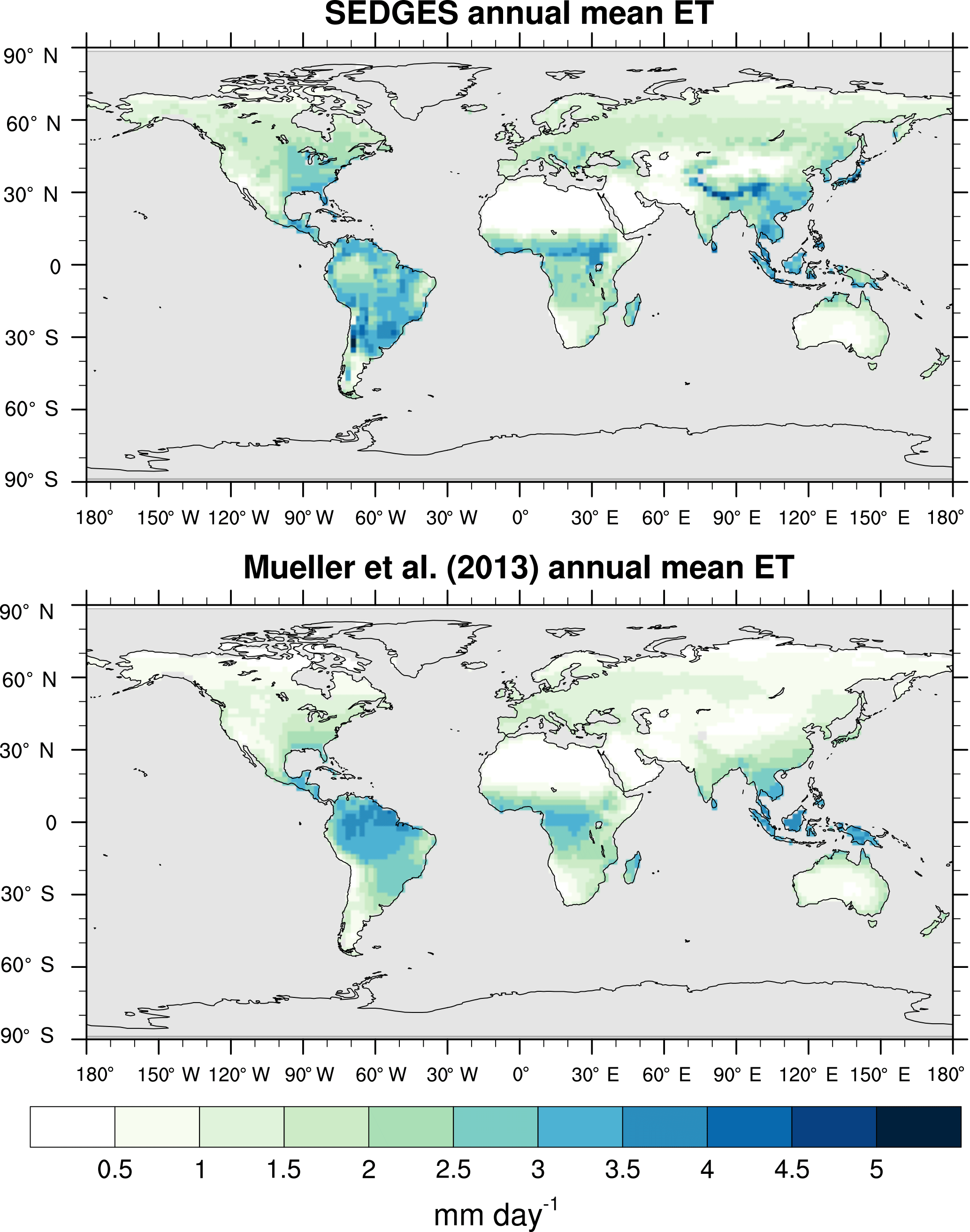
Figure 15 Multiyear annual means of ET for SEDGES and the Mueller et al. (2013) reference dataset for the 1989–2005 period over non-glaciated land.

5.6 Evaluation of evapotranspiration and runoff

Evapotranspiration from SEDGES is compared to that of a multisource compilation reference dataset, Mueller et al. (2013), for the period from 1989 to 2005. Simulated evapotranspiration by SEDGES qualitatively follows that of the reference dataset, successfully capturing the first-order seasonal zonal mean pattern and annual pattern (Figs. 3 and 15). Some salient deficiencies exist, however.

Globally, the annual means in Figs. 3 and 15 show that ET is excessive, overall. Future versions of SEDGES will improve this bias, possibly through the inclusion of a more realistic treatment of the ratio of intercellular to atmospheric CO₂ $\left(\frac{c_{\mathrm{i}}}{c_{\mathrm{a}}}\right)$ instead of the currently fixed value of 0.80, which is probably too high, in general. The important role of $\frac{c_{\mathrm{i}}}{c_{\mathrm{a}}}$ in transpiration is discussed more below and in Sect. 6. On the other hand, the percentage of global evapotranspiration coming from transpiration is 64 % in SEDGES, which compares very well with a literature-based estimate of 61 % (with 15 % standard deviation), derived from 81 studies (Schlesinger and Jasechko, 2014).

Figure 16 July mean ET for SEDGES and the Mueller et al. (2013) reference dataset for the 1989–2005 period over non-glaciated land.

Regionally, the most severe discrepancy from the Mueller et al. (2013) reference dataset is the excessive ET simulated by SEDGES in the mid- to high northern latitudes, which is most pronounced in the transition season from late winter to early spring (Fig. 3). This ET bias occurs because the new parameterization (see Sect. 2.2.5) to reduce excessive sublimation from snow-covered surfaces in the original SimBA parameterization is only moderately effective. This deficiency is possibly the most crucial one to improve in future model versions, possibly by implementing a scheme to decrease surface roughness from snow-covered terrain (e.g., Cox et al., 1999). Another major contributor to the mid- to high northern-latitude positive ET bias is the absence of winter-deciduous leaf phenology and the assumed instantaneous temperature acclimation in SEDGES (Appendix Appendix A), which together increase spring GPP (Sect. 5.1) and thus, concomitantly, increase transpiration. Additionally, Fig. 16, which shows July ET for SEDGES and the Mueller et al. (2013) dataset, suggests that snow-free bare-soil evaporation from moist areas is excessive, as indicated by the relatively large positive ET biases in the high northern latitudes, which have a large contribution to total ET from soil evaporation due to their moist soils and low LAI (Fig. 13) (and hence low leaf cover fraction).

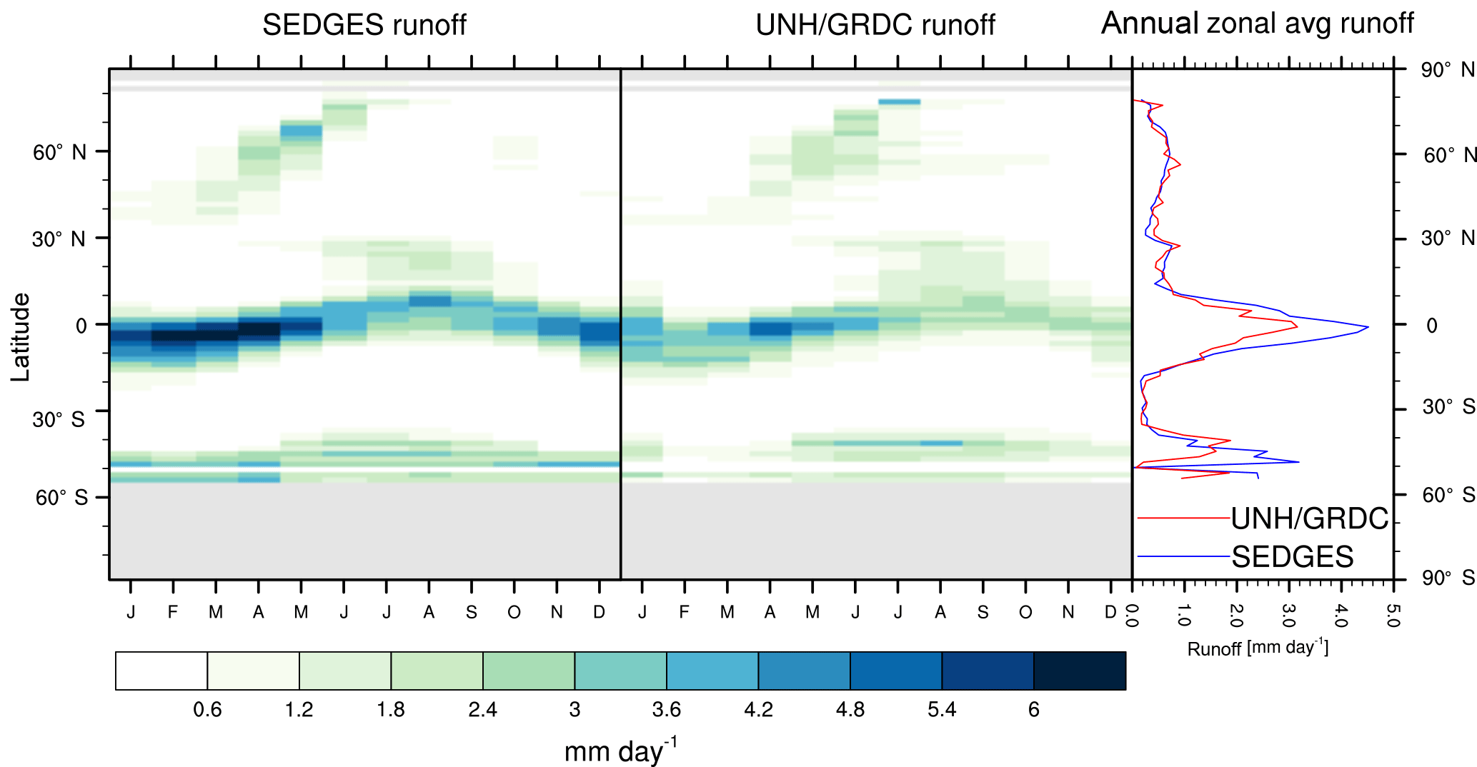
Figure 17 Zonal monthly mean and zonal annual mean climatologies of runoff for SEDGES and the UNH-GRDC reference dataset (Fekete et al., 2002) over non-glaciated land.

In addition to the northern mid- to high-latitude positive bias, SEDGES suffers from a negative ET bias in the equatorial region (Fig. 3), which has at least three likely causes. A positive bias in annual cloud cover fraction in the ERA-Interim data (Dolinar et al., 2016) results in a negative bias in the incident surface shortwave radiation field (Zhang et al., 2016) on the order of ≈ 5 to 30 % throughout most of the equatorial tropics for at least 6 months of the year. This bias may result in a relative reduction in GPP of similar magnitude in SEDGES, which would help to explain the negative GPP bias that SEDGES simulates here (seen in Figs. 5 and 6), while also explaining a reduction in transpiration of comparable (but lesser) magnitude. The latter would result from the increased canopy resistance (Eq. 13) that would ensue from the decreased demand for CO₂ uptake due to the lower light. The lack of an increase in light use efficiency under cloudy skies in SEDGES further exacerbates the negative GPP bias caused by the surface shortwave reduction (see Sect. 6 for more discussion). The second reason for low ET near the equator is the complete absence of canopy interception loss in SEDGES, since this source of surface evaporation has been found to comprise around 20 % of total ET in tropical rain forests (Shuttleworth, 1988; Da Rocha et al., 2004; Czikowsky and Fitzjarrald, 2009; Miralles et al., 2011).¹¹ Finally, the low vapor pressure deficits in the wet tropics do not activate a mechanism in SEDGES that, in other models, would increase transpiration. Less transpiration is simulated by SEDGES in this region because SEDGES's simplifying assumption of a fixed $\frac{c_{\mathrm{i}}}{c_{\mathrm{a}}}$ promotes underestimation (overestimation) of transpiration when vapor pressure deficits are low (high), due to the increase in $\frac{c_{\mathrm{i}}}{c_{\mathrm{a}}}$ with decreasing vapor pressure deficit (Medlyn et al., 2011, 2012; Prentice et al., 2014). It then follows from Fick's law of diffusion (on the plant scale) that higher $\frac{c_{\mathrm{i}}}{c_{\mathrm{a}}}$ decreases the leaf-to-air CO₂ gradient, thus requiring that stomatal conductance increase to ensure sufficient CO₂ inflow for photosynthesis. The higher stomatal conductance increases transpiration. A similar process happens on the canopy scale.

Conspicuously high ET can be seen toward the end of the wet season at both the northern and southern edges of the tropics in Fig. 3. A very similar zonal mean temporal pattern is found in transpiration in the STEAM (Simple Terrestrial Evaporation to Atmosphere Model) land surface model (Fig. 6 of Wang-Erlandsson et al., 2014). Because this model was evaluated using ERA-Interim forcing data, the high ET anomalies that we see in Fig. 3 may be attributable to this particular forcing; the ET anomalies in SEDGES may also be attributable to the lack of canopy interception loss, which declines in tandem with precipitation toward the end of the wet season in Wang-Erlandsson et al. (2014), thus reducing the magnitude of the ET aberrations.

On a smaller regional scale, areas of complex terrain and topography (the Andes and the Himalayas) have very strong positive annual mean ET biases (Fig. 15). We believe that this is an interpolation artifact stemming from cold, snow-covered grid cells lying adjacent to warm, snow-free grid cells. With the spatial interpolation of ERA-Interim to the coarse T62 resolution, such cases often result from deep snow being distributed over the entire area and having a relatively warm temperature due to the influence of the low-lying grid cells at the original high resolution. This setup results in strong evaporation.

With respect to other models of similar complexity, SEDGES simulates ET much better than the original SimBA (see Appendix Appendix C). However, at least when looking at the climatological annual mean, ET is considerably better-simulated by ENTS (Williamson et al., 2006) than by SEDGES. In general, ENTS has a negative ET bias in dry regions and a positive bias in moist regions, especially in parts of the tropics. However, these deviations are generally no greater than the biases that SEDGES has.

Simulated runoff is compared to the composite gridded dataset from the University of New Hampshire (UNH) and World Meteorological Organization's Global Runoff Data Centre (GRDC) (Fekete et al., 2002). SEDGES simulates runoff well except for excesses in the equatorial tropics and in the midlatitudes of the Southern Hemisphere (Fig. 17), especially in equatorial Africa and in the Andes (Fig. 18). Excessive runoff in the equatorial tropics is due to the aforementioned negative ET bias, but it is also attributable to a general overestimate of precipitation in these latitudes by ERA-Interim, especially in equatorial Africa (Lorenz and Kunstmann, 2012; Dolinar et al., 2016). Global runoff for SEDGES, excluding areas of land ice, is about 44 ×10¹⁵ kg yr⁻¹, which is slightly higher than the 38 ×10¹⁵ kg yr⁻¹ for the UNH/GRDC dataset and the global (excluding Antarctica) runoff estimate of 37 ×10¹⁵ kg yr⁻¹ by Dai and Trenberth (2002).

It should be noted that the parameterization for soil water-holding capacity (Sect. 2.3.2) gives generally much lower values (not shown) in the wet and dry tropics than in the reference dataset (Kleidon and Heimann, 1998; Hall et al., 2006; Kleidon, 2011). Such lower values of soil water-holding capacity should lead one to expect a positive runoff bias in these areas in SEDGES. This is not the case, however, when we compare those regions of the wet and dry tropics where the ERA-Interim precipitation forcing has insignificant bias (and where biases in SEDGES runoff are thus unlikely to be attributable to precipitation deficiencies in the forcing). The lack of runoff bias in these regions suggests that the parameterization of soil water-holding capacity in SEDGES (Eq. 28) works well in tandem with its ET scheme and the simple soil bucket hydrology (Eq. 31).

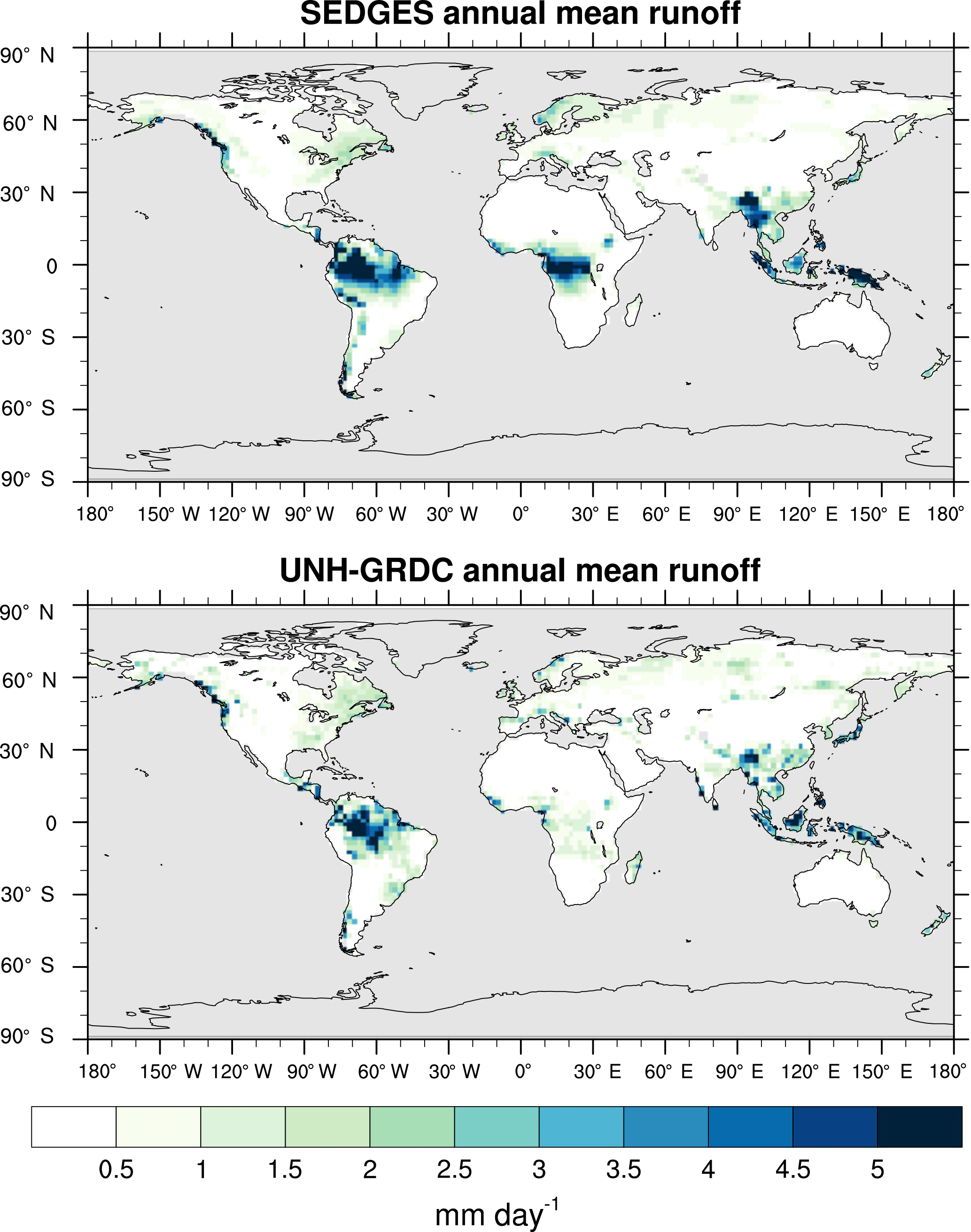
Figure 18 Climatological annual mean of runoff for SEDGES and the UNH-GRDC reference dataset (Fekete et al., 2002) over non-glaciated land.

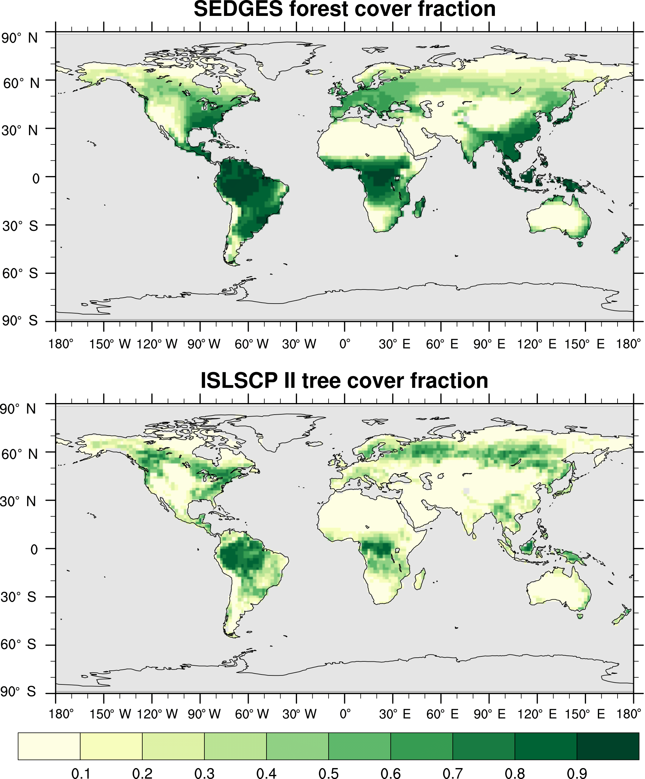
Figure 19 Mean forest cover fraction for SEDGES and tree cover fraction from the reference ISLSCP II dataset (DeFries and Hansen, 2009).

Finally, while it might seem easy to attribute deficiencies in the SEDGES hydrology to our use of the single-layer soil bucket, this type of model has been found to perform well under many conditions: wet soils, when precipitation events tend to be large relative to the bucket depth, and under strong root compensation or hydraulic redistribution of soil moisture (Guswa et al., 2002; Guswa, 2005). Even when the aforementioned conditions do not hold, distortions stemming from the use of the single-layer bucket model are comparable to those coming from other aspects of SEDGES hydrology.

5.7 Evaluation of forest cover fraction

The overall global pattern of tree cover fraction of the International Satellite Land Surface Climatology Project (ISLSCP II) reference dataset (DeFries and Hansen, 2009) is captured reasonably well by SEDGES, as seen from Fig. 19. However, SEDGES has almost double the amount of arboreal cover. In Europe, China, and India, this is at least partially due to anthropogenic land cover change of natural forests and woodland to croplands (Ramankutty and Foley, 1999). Aside from this deforestation, the model's lack of competing plant functional types (especially boreal trees, warm region trees, and grasses) in conjunction with the constant residence time of 10 years for all vegetative carbon, leads to an overestimation of arboreal vegetation by SEDGES in South America, Africa, and North America, as well as a slight underestimation in boreal forest regions. A noted limitation of the reference dataset is its underestimation of real-world tree cover in areas with the highest cover fraction. Thus, SEDGES's overestimates in these regions may partially be due to this phenomenon, as well. Finally, a less inclusive definition for arboreal cover in the reference dataset than in SEDGES contributes to the cover overestimate in the latter. SEDGES assumes that forest is vegetated land that protrudes above the winter snowpack, whereas the ISLSCP II dataset requires that trees be at least 5 m tall to count toward tree cover and thus excludes short trees and tall shrubs that do not get completely buried by snow.

5.8 Model evaluation: summary and conclusions

The performance of the new SEDGES model has been evaluated for the present day through comparison with numerous reference land datasets. To do this, we have forced SEDGES offline with ERA-Interim data, using our recommended simple single-layer bucket soil hydrology to simulate terrestrial water storage, incorporating a simple scheme to handle a snow-temperature mismatch in the forcing data, and adopting the Planet Simulator's formulation for aerodynamic conductance. Note that the particular forcing data and hydrological implementations impact the analyzed output of the SEDGES simulations. In particular, the spin-up using repeated climatology from 1981–2010 yields conditions that differ from a spin-up using purely historical data. Not only do forcing and hydrology affect the model evaluation, but so do the reference datasets against which it is compared, since even they are not perfect representations of reality. Given all of these particularities, one must view the presented evaluation as a conditional, non-definitive, but yet informative guide to the strengths and the weakness of the model.

The following output variables of SEDGES have been examined: GPP, vegetative carbon, soil organic carbon, LAI, surface albedo, ET, runoff, and forest cover fraction. In comparison to the respective reference datasets, SEDGES simulates each variable at least reasonably well. Relative model strengths lie in the simulation of GPP; relative weaknesses in ET, snow-free albedo, and forest cover fraction. Given the simplicity of its formulation, the strength in GPP is unexpected, particularly the ability of SEDGES to capture the spatial patterns of temporal trends in GPP. Simulated ET is too high in the mid- to high northern latitudes and is too low in the wet tropics. SEDGES captures albedo patterns fairly well outside of boreal summer, but subtler differences among the different desert types and among the nondesert areas are not well-captured during the snow-free season. Simulated forest cover fraction is generally too high.

6 Discussion and conclusions

A new simplified model for the representation of dynamic ecological processes for use in conjunction with climate models has been developed. This new model was combined with a simple hydrological scheme and forced with reanalysis data. In evaluating its performance, we concentrated on the comparison with present-day observation-based data products, while also referring to land surface models (especially ENTS) and their performances for a relative comparison of the strengths and weaknesses of SEDGES.

The quantitative comparison highlighted strengths and weaknesses of the model. A notable strength is that SEDGES's simulation of gross primary productivity is comparable to and sometimes better than that of state-of-the-art dynamic global vegetation models. Our evaluation has also shown that SEDGES performs well in a number of other metrics. Overall, the results show that SEDGES can be used to adequately simulate modern land surface characteristics, including input variables to land–atmosphere coupling schemes used in climate models, as well as key variables of the hydrological and terrestrial carbon cycles.

The most severe weaknesses of our offline-run SEDGES are the aforementioned strong positive ET bias that it yields in the mid-to-high latitudes in winter and early spring and its overprediction of arboreal cover. The latter results from the use of only one plant functional type, which carries over from the SimBA model, on which SEDGES is based. Even an expansion to just two plant functional types (e.g., tree and herbaceous) and simulation of competition between them would entail a significant increase in model complexity. However, SEDGES's use of only one plant functional type, along with a fixed relationship between biomass and both wet-soil LAI and rooting depth hydrology, excessively constrains large-scale vegetation structure by excluding the emergence of location-adapted landscape characteristics. As a result of these issues, simulated vegetation in water-limited regions and wetness-induced changes in biomass should be treated as more heuristic than definitive. Returning to ET, although less severe, the positive ET bias is also seen in the mid-to-high latitudes during the snow-free season. In contrast, the equatorial tropics have a strong negative ET bias due to high cloud cover and concomitant low insolation, which increases canopy resistance and thus reduces transpiration (as seen in Eq. 13). This negative bias occurs for various reasons, including SEDGES's lack of distinction between sunlit and shaded leaves (see below), lack of evaporation from canopy-intercepted water in SEDGES (see Sect. 5.6 for more), and a positive cloud cover and a negative surface insolation bias in the forcing dataset (see Sect. 5.6 for more). The last of these may also be associated with further reductions in transpiration by way of a more stable and humid boundary layer, which would decrease the specific humidity difference between the surface and the lower atmosphere (Δq) and increase the aerodynamic resistance (r_a) in Eq. (13). Regardless, ET would be less inhibited by these cloudy and humid conditions if the ratio of intercellular to atmospheric CO₂, $\frac{c_{\mathrm{i}}}{c_{\mathrm{a}}}$, were given a more realistic treatment that is in line with recent theoretical development and measurements pertaining to optimized stomatal conductance (Medlyn et al., 2011; Prentice et al., 2014; Lin et al., 2015); such treatment is already occurring in some land surface models (e.g., De Kauwe et al., 2015; Kala et al., 2015; Willeit and Ganopolski, 2016). The new theory formalizes how and why, at the leaf level, $\frac{c_{\mathrm{i}}}{c_{\mathrm{a}}}$ increases/decreases with decreased/increased vapor pressure deficit (VPD) (which is approximately proportional to Δq). Because CO₂ uptake is proportional to $\mathrm{1}-\frac{c_{\mathrm{i}}}{c_{\mathrm{a}}}$ (Eq. 6), increased $\frac{c_{\mathrm{i}}}{c_{\mathrm{a}}}$ results in decreased canopy resistance (in order to maintain the same level of CO₂ uptake, i.e., match the light-limited rate of GPP), which results in decreased transpiration (Eq. 13) (unless transpiration is occurring at the maximum rate).

The implementation of variable $\frac{c_{\mathrm{i}}}{c_{\mathrm{a}}}$ was not made in SEDGES because the simple relationships between $\frac{c_{\mathrm{i}}}{c_{\mathrm{a}}}$ and VPD that are derived from optimization principles (Medlyn et al., 2011, 2012; Prentice et al., 2014) are incompatible with the SEDGES framework. The derivations for optimized $\frac{c_{\mathrm{i}}}{c_{\mathrm{a}}}$ both assume a Fick's law of diffusion transmission between the leaf and the outside air. In order to have consistency in moisture and CO₂ fluxes between the land surface and atmosphere, the land surface scheme also needs to use a diffusive exchange between outside air and leaves, or at the least, to reasonably approximate such diffusive exchange. Diffusive exchange of moisture and CO₂ is not used in the SEDGES framework. Instead, transfer occurs from surface to atmosphere through a bulk aerodynamic formulation. This formulation only approximates the purely diffusive scheme when canopy resistance (r_c) greatly exceeds aerodynamic resistance (r_a). As is said in Sect. 2.2.4, in early versions of SEDGES (coupled to Planet Simulator), it was found that this condition (r_c≫r_a) was frequently violated. That said, in light of the aforementioned ET biases, we intend to incorporate variable $\frac{c_{\mathrm{i}}}{c_{\mathrm{a}}}$ in future versions of SEDGES. Note that it is not enough to simply adjust the globally fixed $\frac{c_{\mathrm{i}}}{c_{\mathrm{a}}}$ in the current model to resolve the ET problems because doing so would improve the bias in the mid- to high latitudes while worsening it in the equatorial tropics (or vice versa).

The use of a fixed value of $\frac{c_{\mathrm{i}}}{c_{\mathrm{a}}}$ is likely to play a more important role in transpiration (by way of affecting the water-use efficiency) than in GPP under non-water-limiting conditions (i.e., when GPP = GPP_L, where GPP_L is the light-limited rate of GPP (Sect. 2.2.3)). This is because, when r_c≫r_a (i.e., using the diffusive approximation for heuristic purposes), transpiration is proportional to $\mathrm{\Delta }q{\mathrm{GPP}}_{\mathrm{L}}/\left(\mathrm{1}-\frac{c_{\mathrm{i}}}{c_{\mathrm{a}}}\right)$. As such, changes in $\frac{c_{\mathrm{i}}}{c_{\mathrm{a}}}$ (whose values are typically closer to 1 than 0 for C₃ plants) have greater relative impact on transpiration than they do in the equations for either RuBP (ribulose 1,5-bisphosphate) regeneration-limited or Rubisco-limited photosynthesis (at least for non-extreme conditions) in the Farquhar model (Farquhar et al., 1980). Furthermore, explicit dependence on $\frac{c_{\mathrm{i}}}{c_{\mathrm{a}}}$ is not critical when modeling GPP. In remote-sensing applications, light use efficiency models without explicit c_i dependence have been widely successful in modeling GPP for many years (e.g., Yuan et al., 2007, and references within). An inter-model comparison between the aforementioned light use efficiency models and the explicitly c_i-dependent enzyme-kinetic-based approaches (Schaefer et al., 2012) shows that including explicit c_i variation (and hence $\frac{c_{\mathrm{i}}}{c_{\mathrm{a}}}$ variation) does not apparently improve the modeling of GPP. On the other hand, for arid regions in which water supply is often limiting, the decrease in $\frac{c_{\mathrm{i}}}{c_{\mathrm{a}}}$ and concomitant increase in water-use efficiency (GPP per amount of transpired water) affects GPP somewhat strongly.

As the SEDGES model was developed, many of the formulations were calibrated, both independently and dependently of model simulations. As noted by Foley et al. (2013), model calibration should ideally be done separately from model evaluation, but this happens only rarely in practice. In this paper, some of the datasets that were most heavily relied on for calibration were also used for model evaluation. These include the MODIS albedo dataset (NASA LP DAAC, 2008b), the MTE GPP dataset (Jung et al., 2011) (multiyear annual mean), the Mueller et al. (2013) ET dataset (multiyear annual mean), and the BNU MODIS-based LAI dataset (Yuan et al., 2011). The least well-constrained parameters and relationships that SEDGES is sensitive to are the ϵ_max, the soil organic carbon value at which soil albedo saturation occurs (c₇), the trmax, the CO₂ fertilization function, the low-temperature limitation function, and c₄ and c₅ in the relationship between biomass and snow-covered albedo. The model is only moderately sensitive to the c₁₂ parameter, which governs the relationship between biomass and the soil bucket depth. The “representative” value for $\left(\frac{c_{\mathrm{i}}}{c_{\mathrm{a}}}\right)$ is also somewhat unconstrained (e.g., see Prentice et al., 2014).

Our offline simulations involving SEDGES and the subsequent comparisons with standard datasets should of course not be considered a complete model evaluation. SEDGES undoubtedly has limitations that cannot be seen from the simulations used in this study. However, from the results of this study and from the formulations that are used in SEDGES, we can anticipate at least some of the situations in which the current model might perform less realistically and/or suggest how to modify SEDGES for these cases.

In Sect. 2.2.3, for the calculation of the light-limited rate of GPP (Eq. 2), ϵ_max is the same regardless of the diffuse or direct nature of the absorbed solar radiation. However, this lack of distinction is questionable, as shown by two observation-based studies on the relationship between the diffuse fraction of SW (shortwave) radiation at the top of the canopy and LUE that control for the negative correlation between VPD and diffuse SW fraction in their results (Alton et al., 2007; Williams et al., 2014). When going from conditions of predominantly direct solar radiation to predominantly diffuse solar radiation, Alton et al. (2007) finds an observed 6 to 33 % increase in LUE in three forests, whereas Williams et al. (2014) finds an ≈ 17 % increase in LUE in shrub tundra. The increase in LUE is apparently due to a more even distribution of PAR among the leaves, which reduces light saturation among the sunlit leaves. The distinction between sunlit and shade leaves is missing in our model's single big-leaf approach to canopy radiation, which tacitly assumes a spatially averaged light profile at each level of the canopy (de Pury and Farquhar, 1997; Monson and Baldocchi, 2014, p. 355). Not including a sunlit/shade leaf distinction implies that, in the absence of water limitation, our model underpredicts GPP at low sun angles and under cloudy conditions (and overpredicts it for opposite conditions). This pattern is, in fact, reflected in the regional negative GPP biases that are mentioned in Sect. 5.1, with negative productivity biases occurring in regions with reduced downwelling surface SW radiation for their latitude (in the reanalysis), especially in the equatorial tropics. Recent studies show that including a sunlit/shade leaf distinction reduces errors in the simulation of GPP (Yuan et al., 2014; Wu et al., 2015) (but cf. Schaefer et al., 2012). Thus, in a future version of SEDGES, we hope to incorporate the sunlit/shade leaf distinction.

Although gross photosynthesis is somewhat robust to changes in elevation (i.e., atmospheric pressure), there is an appreciable decline at high altitudes and high temperature (Terashima et al., 1995) (according to the widely used Farquhar model; Farquhar et al., 1980), which should affect places like the Tibetan Plateau and the South American Altiplano. In these regions, the calculations by Terashima et al. (1995) suggest that SEDGES would overestimate the rate of its light-limited gross primary productivity (Eq. 2) by ≈ 20 % and by potentially more for areas in these regions that have low biomass (since these would have a stronger feedback between leaf cover fraction and productivity).

Also in Sect. 2.2.2, we stated that SEDGES approximates net primary productivity as half of gross primary productivity (NPP ∕ GPP = 0.5), while noting that this approximation is only valid on the timescales of weeks or longer. On shorter timescales, the ratio may deviate substantially from 0.5, due to the strong short-term dependency of autotrophic respiration on temperature (e.g., Monson and Baldocchi, 2014), and, as such, carbon uptake by the land surface may not be well-simulated on these short timescales.

With respect to simulating terrestrial carbon pool changes, SEDGES's use of a single soil organic carbon reservoir and its fixed residence time for vegetative carbon may also need to be considered when drawing inferences from model results in transient simulations (e.g., see Friend et al., 2014).

These last issues with regards to the carbon cycle are part of a group of model deficiencies in simulating some ecological dynamics. Of these simulation deficiencies, the most severe are probably of the phenological changes (GPP, NPP, transpiration, and especially LAI) associated with green-up in the Northern Hemisphere. More generally, however, it is likely that simplifying assumptions made by SEDGES (namely, constant NPP ∕ GPP as well as its universal temperature limitation function; Appendix Appendix C) lead the model to overestimate the capacity of vegetation to adapt to rapidly changing conditions, especially on daily timescales. As such, SEDGES may underestimate the less positive impacts of extreme weather events on vegetation.

In paleoclimate simulations, periods before the Paleogene may require the modification of SEDGES due to differences in atmosphere oxygen concentration and to the effect of evolution on large-scale plant characteristics and behavior. SEDGES tacitly assumes an atmospheric oxygen concentration near its present-day value of ≈ 21 % in both the ϵ_max and in the light compensation point in the absence of dark respiration $\left({\mathrm{CO}}_{{\mathrm{2}}_{\mathrm{comp}}}\right)$. However, ${\mathrm{CO}}_{{\mathrm{2}}_{\mathrm{comp}}}$ is proportional to the O₂ concentration in the atmosphere (e.g., p. 102 of Monson and Baldocchi, 2014), which, in turn, affects the CO₂ fertilization effect in SEDGES (Eq. 3). Higher/lower O₂ would lead to greater/lesser fertilization. Next, for a given CO₂ concentration, higher O₂ increases photorespiration and decreases gross photosynthesis, both experimentally and according to the aforementioned Farquhar model (Beerling et al., 1998) (although the effect was also found to be less pronounced for evolutionarily older taxa). These results suggest that ϵ_max should be lowered/raised in SEDGES for higher/lower-than-present atmospheric O₂ levels. (In addition, although optimization theory by Prentice et al. (2014) and experimental measurements show that the ratio of intercellular to atmosphere ${\mathrm{CO}}_{\mathrm{2}}\left(\frac{c_{\mathrm{i}}}{c_{\mathrm{a}}}\right)$ increases/decreases with higher/lower atmospheric O₂, the increase is found to be only ≈ 0.06 when going from the current (21 %) to the extreme high (35 %) O₂ level over the last 400 million years (Beerling et al., 1998). This $\frac{c_{\mathrm{i}}}{c_{\mathrm{a}}}$ difference is small in comparison with other uncertainties and inaccuracies in the model and can thus probably be neglected.)

Apart from the effects of changing atmospheric O₂ concentration, vegetation characteristics important to the large scale have evolved and changed along with the Earth, and this fact has been recognized by previous researchers (e.g., by excluding plant functional types that have not yet evolved in paleoclimate simulations (e.g., Horton et al., 2010; Zhou et al., 2012)). We recommend making changes in line with a recent review of climate-relevant changes in plant physiology on geological timescales (Boyce and Lee, 2017). From the early Paleozoic to the Early Devonian, the landscape was dominated by nonvascular vegetation that lacked stomatal control over water loss, substantial roots, and tree-like aboveground structures. In order to simulate a landscape with this kind of vegetation, canopy resistance (r_c) should be set to near 0, W_max should be set to its minimum value ($W_{{max}_{min}}$) (regardless of biomass), and the biomass residence time τ_veg should be decreased as needed to keep the highest biomass from going above 1.0 kg C m⁻². Starting with the landscape dominance by vascular plants in the Carboniferous, modern-like landscapes of forests, deep-rooted vegetation, and stomatal control over water loss were widespread, and the current version SEDGES should be able to adequately simulate the vegetation of these geological times (provided that the aforementioned effects of differing O₂ are included). The Middle and Late Devonian saw the development and expansion of vascular plants and would require a more in-depth analysis on how to properly simulate with SEDGES because it represents a transition between the two aforementioned time periods.

It is important to realize that this paper has focused on SEDGES forced offline, i.e., not fully integrated into a climate or Earth system model. While a stand-alone evaluation against present-day observations or in comparison with other models is not sufficient to make firm statements on how SEDGES would perform in a coupled mode, it is beyond the scope of this paper to evaluate SEDGES within a coupled climate or Earth system model. Nevertheless, the performance of SEDGES in a coupled system will need careful evaluation. First results with the coupled PlaSim-SEDGES model are discussed in Paiewonsky (2017). In general, it is to be expected that coupling may exacerbate or reduce biases present in the offline mode of SEDGES that has been evaluated in this paper. For example, the aforementioned ET biases that SEDGES has (Sect. 5.6) are likely to be diminished through a long-known negative feedback (e.g., Sato et al., 1989): excessive ET moistens and stabilizes the boundary layer which reduces the specific humidity difference between the surface and the lower atmosphere (lowers the Δq and increases the r_a in Eq. 7), thus reducing ET and thus feeding back negatively onto the original positive ET bias. On the other hand, there are two notable positive feedbacks that may occur in coupled mode. First, the positive snow-free surface albedo bias in the high Arctic in SEDGES (e.g., see July in Fig. 4) may feed back positively in these regions and worsen the initial bias by cooling the surface, thus reducing productivity, thus reducing soil organic carbon, and thus increasing the surface albedo. Second, through another albedo mechanism in boreal spring (the forest–tundra snow albedo feedback, e.g., Bonan et al., 1992; Foley et al., 1994), the high albedo bias in northern Siberia'a forest–tundra woodland zones would be expected to lead to additional cooling in this region, thus further reducing productivity, thus decreasing biomass, and thus increasing the snow-covered surface albedo, resulting in an exacerbation of the initial positive albedo bias in this region.

For its level of complexity, SEDGES and the land surface framework which it presupposes have the advantages of a flexible time step, canopy control over transpiration, transpiration that is fully coupled to photosynthesis, and vegetative productivity that depends on light and not just temperature and moisture. The short time step option permits SEDGES to be incorporated into models that resolve the diurnal cycle. Because of these strengths, we expect SEDGES to have advantages over vegetation models of similar complexity in simulating vegetation, primary productivity, and transpiration in past geological warm periods in regions that receive little sunlight (e.g., the Eocene Arctic; Maxbauer et al., 2014, and references within) and in simulating cloud–vegetation feedbacks in all eras. The SEDGES framework uses photosynthetic-driven stomatal control over evapotranspiration, which is critical when studying hydrological changes on land under altered atmospheric CO₂ concentrations, including anthropogenically induced warming scenarios (Betts et al., 2007).

The SEDGES framework has the advantages of being easier to understand, process-wise, than more complex vegetation and hydrological schemes. Increased vegetation model complexity can obfuscate model behavior, and it need not improve performance. In an inter-model comparison of the performance of 24 vegetation models at 39 eddy covariance flux tower sites, Schaefer et al. (2012) finds insignificant effects of nitrogen cycle inclusion and of having a light use efficiency or enzyme kinetic approach to productivity on a model's capacity to simulate GPP. Moreover, even when present-day biome distributions are well-simulated by complex vegetation models, model behaviors can diverge drastically from each other under non-present conditions due to differing physiological assumptions (e.g., climatic limitations within plant functional types) that are not well-grounded and that may very well change under novel climatic, atmospheric CO₂, and nutrient conditions (Fisher et al., 2015).

In conclusion, we feel that SEDGES provides a new viable and computationally efficient alternative to currently implemented terrestrial vegetation/ecological models, in particular inside Earth system models of intermediate complexity and for research on the global-scale interactions between the physical climate system and the terrestrial biosphere.

Appendix A: Notes on the temperature limitation function

In this section, we discuss the rationale behind our particular temperature limitation multiplier, f₂(T_sfc), on the light-limited rate of gross primary productivity (Eq. 2) in Sect. 2.2.3.

f₂(T_sfc) increases linearly from 0 at T_sfc of 0 ^∘C to 1 at T_sfc of 20 ^∘C and then plateaus at 1. The linear increase is chosen for its simplicity and because it is analogous to the often-used “growing degree days” (GDDs) metric (with 0 ^∘C base) in agriculture and ecology (Kauppi and Posch, 1985; Prentice et al., 1992; Kaplan, 2001) (save for the shorter timescale). SEDGES's critical temperature of 20 ^∘C at which productivity is no longer limited lies close to the middle of the range of optimum temperatures for C3 plants (5–39 ^∘C) that was found in a survey of 212 temperature response curves of photosynthesis in the literature for different species and growth temperatures (Way and Yamori, 2014; Yamori et al., 2014). While the critical temperature for the Kleidon (2006b) SimBA model is 5 ^∘C, it otherwise uses the same ramp function formulation as SEDGES.

Figure A1 Multiyear annual mean of GPP for the original SimBA model (Kleidon, 2006b) and the two reference datasets, MTE and CARBONES, for 1990–2009 over non-glaciated land.

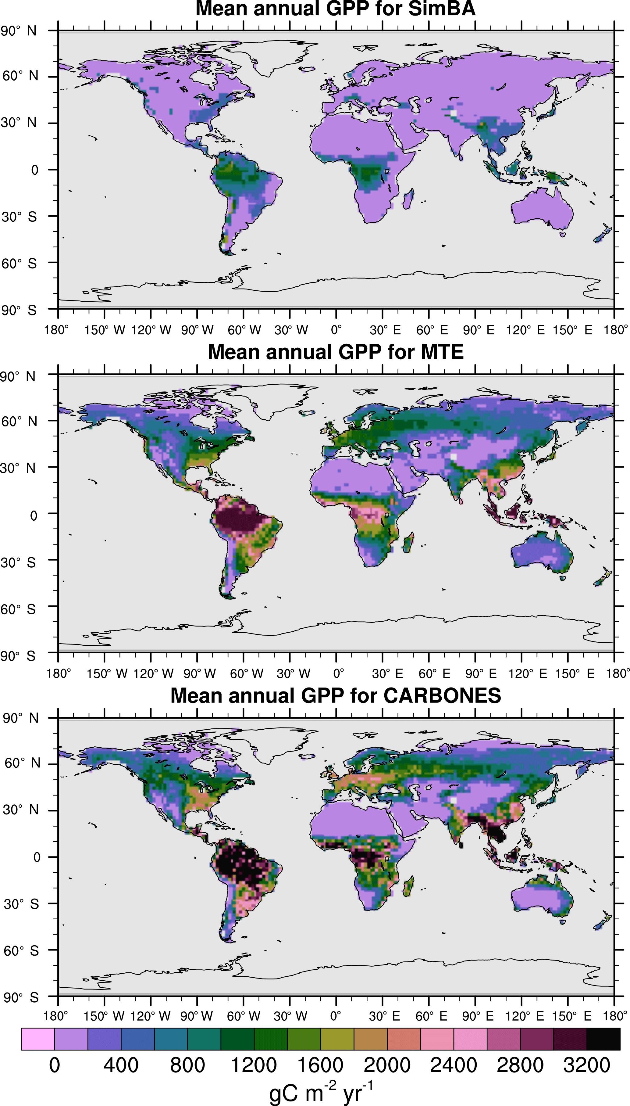
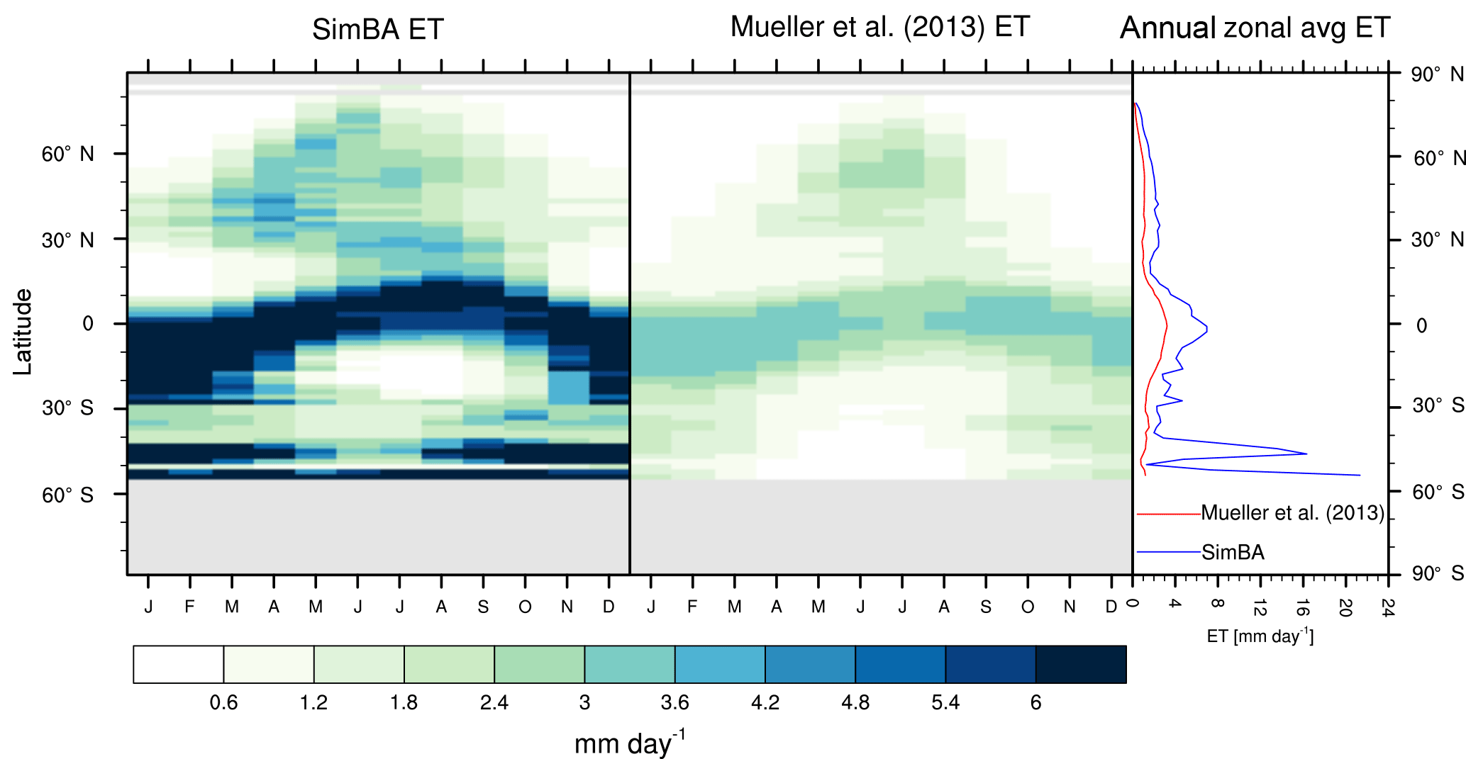
Figure A2 Zonal multiyear monthly means and zonal multiyear annual means of ET for the original SimBA model (Kleidon, 2006b) and the Mueller et al. (2013) reference dataset for the 1989–2005 period over non-glaciated land.

Temperature limitation on photosynthesis has been well studied (e.g., see reviews by Sage and Kubien, 2007; Yamori et al., 2014), but many uncertainties remain. In land plants, photosynthesis is significantly limited by both high and low temperatures. Individual plants of different species and from different environments have differing optimal temperatures for photosynthesis, such that away from the optimal temperature, photosynthetic rate decreases (Yamori et al., 2014). Around the temperature optimum, there exists a range of temperatures for which photosynthesis is nearly as high as at the optimum (Berry and Bjorkman, 1980; Yamori et al., 2014). Both the temperature dependency and the maximum rate of photosynthesis (realized at the temperature optimum) can shift as a plant acclimates to a different set of environmental conditions (Berry and Bjorkman, 1980; Way and Yamori, 2014; Yamori et al., 2014).

In most plants, temperature limitation on photosynthesis depends on the species, current light levels, the environmental conditions under which the plant grew, and the internal levels of CO₂ in the leaves (Berry and Bjorkman, 1980; Sage and Kubien, 2007; Way and Yamori, 2014; Yamori et al., 2014). In addition, the current temperature limitation depends on the extent of acclimation to recent environmental conditions (e.g., Dietze, 2014)

The framework in which we use f₂(T_sfc) assumes perfect acclimation and adaptation of the vegetation to the current weather and light conditions. As such, the SEDGES temperature limitation assumes the presence of the most productive set of plants that could ideally grow under those conditions and also allows for their instantaneous adaptation and acclimation to those conditions. In other words, for a given surface temperature (T_sfc), f₂(T_sfc) represents the universal physiological constraints on productivity exerted by that (isolated) given temperature.

For high temperatures, a conscious decision was made to not include a decline in productivity in SEDGES. Although it is well-established that high temperatures (i.e., temperatures above the optimum) limit productivity for individual plants, some of that limitation that has been found empirically may have been due to an indirect effect of temperature on increasing the leaf-to-air vapor pressure deficit (for constant ambient relative humidity), which causes the optimum temperature to be lower than when the vapor pressure deficit is held fixed (Lin et al., 2012). An even more important point is that a high temperature limitation reflects more the inability of plants that are adapted to a given environment to perform equally well under all conditions that they might face in that environment and less an intrinsic barrier for plant life at that location to adapt to a given high temperature regime (via some combination of species migrations, natural selection, evolution, and/or acclimation). For example, although the Yamori et al. (2014) study found C3 plants to generally have temperature optima between 10 and 35 ^∘C, light-saturated and CO₂-saturated photosynthesis for the C3 hot desert plant, Rhazya stricta, shows no significant decline with leaf temperature even up to 44 ^∘C (Lawson et al., 2014). Moreover, its (ordinary) daily photosynthetic rates are nearly as high as those of common C3 agricultural crops, in spite of living under natural conditions of a much higher vapor pressure deficit and presumably much drier soil (Lawson et al., 2014), which reduce productivity. Similar results as for Rhazya stricta have been found for the C3 desert shrub, Larrea divaricata (Mooney et al., 1978). Thus, the large-scale ability of vascular plant life to adapt to high temperatures through the increased prevalence of heat-tolerant species and phenotypes should be properly accounted for when modeling vegetation and the carbon cycle in past warm climates (such as the Cretaceous) as well as in future climates.

Appendix B: Numerical parameterization of canopy resistance and maximum transpiration rate

Canopy resistance is the greater of an unconstrained canopy resistance ($r_{{\mathrm{c}}_{\mathrm{u}}}$) which is determined by the light-limited rate of canopy photosynthesis (GPP_L) and a canopy resistance set by the maximum rate at which the rooting zone can supply water for transpiration. The equation for the unconstrained canopy resistance is essentially derived by incorporating the canopy resistance (r_c) value from the previous time step, using the mismatch between GPP_W and GPP_L in the last time step, and accounting for updates to the variables that affect GPP_W and GPP_L. Although this formulation of $r_{{\mathrm{c}}_{\mathrm{u}}}$ depends on values from the previous time step, this dependency is arbitrary. An expression for $r_{{\mathrm{c}}_{\mathrm{u}}}$ that depends only on values in the current time step could be derived and used. (Such an $r_{{\mathrm{c}}_{\mathrm{u}}}$ would depend on all the variables that comprise GPP_W and GPP_L, and these variables would be evaluated at the current time step.)

Our starting equation for deriving the unconstrained canopy resistance uses the formulations of GPP_L and GPP_W given in Eqs. (2), (4), (5), and (6) and is as follows:

$$\begin{array}{ll}\text{(B1)}& {\displaystyle }\mathrm{0}\equiv & {\displaystyle }{{\mathrm{GPP}}_{\mathrm{L}}}_{t+\mathrm{1}}-{{\mathrm{GPP}}_{\mathrm{W}}}_{t+\mathrm{1}}{\displaystyle }\approx & {\displaystyle }{\mathrm{GPP}}_{\mathrm{L}}{\displaystyle \frac{f_{\mathrm{leaf}}}{{f_{\mathrm{leaf}}}_{t-\mathrm{1}}}}{\displaystyle \frac{f_{\mathrm{2}}\left(T_{\mathrm{sfc}}\right)}{f_{\mathrm{2}}\left({T_{\mathrm{sfc}}}_{t-\mathrm{1}}\right)}}{\displaystyle \frac{\mathrm{SW}\downarrow }{\mathrm{SW}{\downarrow }_{t-\mathrm{1}}}}\\ {\displaystyle }& {\displaystyle }-{\mathrm{GPP}}_{\mathrm{W}}{\displaystyle \frac{f_{\mathrm{leaf}}}{{f_{\mathrm{leaf}}}_{t-\mathrm{1}}}}{\displaystyle \frac{\mathrm{1.6}{r}_{{\mathrm{c}}_{t-\mathrm{1}}}+r_{{\mathrm{a}}_t-\mathrm{1}}}{\mathrm{1.6}{r}_{{\mathrm{c}}_{\mathrm{u}}}+r_{\mathrm{a}}}}.\end{array}$$

Here, the equivalence statement reflects the first stomatal goal of parsimoniously meeting the light-driven demand for CO₂. The future values of GPP_W and GPP_L are approximated (for simplicity) by neglecting changes in slowly varying variables (e.g., ρ). Equation (B1) represents the standard case for deriving r_c. Special cases are discussed below (e.g., when $f_{{\mathrm{leaf}}_{t-\mathrm{1}}}$, $f_{\mathrm{2}}\left(T_{{\mathrm{sfc}}_{t-\mathrm{1}}}\right)$ or $\mathrm{SW}{\downarrow }_{t-\mathrm{1}}$ are zero.) Solving Eq. (B1) for $r_{{\mathrm{c}}_{\mathrm{u}}}$ yields

$$\begin{array}{ll}\text{(B2)}& {\displaystyle }{r}_{{\mathrm{c}}_{\mathrm{u}}}=& {\displaystyle }\left({\displaystyle \frac{{\mathrm{GPP}}_{\mathrm{W}}}{{\mathrm{GPP}}_{\mathrm{L}}}}{\displaystyle \frac{f_{\mathrm{2}}\left(T_{{\mathrm{sfc}}_{t-\mathrm{1}}}\right)}{f_{\mathrm{2}}\left(T_{\mathrm{sfc}}\right)}}{\displaystyle \frac{\mathrm{SW}{\downarrow }_{t-\mathrm{1}}}{SW\downarrow }}\right.{\displaystyle }& {\displaystyle }(\mathrm{1.6}{r}_{{\mathrm{c}}_{t-\mathrm{1}}}+r_{{\mathrm{a}}_{t-\mathrm{1}}})-r_{\mathrm{a}})/\mathrm{1.6}.\end{array}$$

Equation (B1) has provided us with $r_{{\mathrm{c}}_{\mathrm{u}}}$, the canopy resistance that would occur in the complete absence of physiological limitations on plant water loss. In the real world, plants must restrict how much their stomata open when water cannot be extracted from the soil (or from internal plant storage) and transported to the leaf stomata fast enough to balance the loss to the atmosphere through the stomata. Doing so helps to keep water potentials within the plant from falling to levels that would cause “runaway” cavitation (Tyree and Sperry, 1988) or “hydraulic failure” (McDowell et al., 2008). Closing stomata increases stomatal resistances across the leaves, which, on the canopy scale, increases the canopy resistance. In this way, canopy resistance can be constrained by the supply rate of water from the soil to the leaves.

To simulate the maximum supply rate of water for transpiration, SEDGES adapts the simple model of Federer (1982). The original Federer maximum supply rate is directly proportional to the soil wetness fraction multiplied by a fixed constant parameter. This parameter is the absolute maximum transpiration value, which we denote here by trmax. In SEDGES, we extend the original Federer formulation from the limited case of a fully vegetated surface to the case of a mixed surface comprised of green leaves and exposed soil. This is achieved by simply multiplying the original expression by the leaf cover fraction, f_leaf. Thus, the supply rate for transpiration, S_tr, is as follows in SEDGES:

$$\begin{array}{}\text{(B3)}& S_{\mathrm{tr}}=f_{\mathrm{leaf}}\cdot {\mathit{\beta }}_{\mathrm{tr}}\cdot \mathrm{trmax},\end{array}$$

where β_tr is a water stress factor that affects the roots' ability to supply water for transpiration and equals the soil wetness fraction, W_frac, and trmax has a value of $\mathrm{2.78}\times {\mathrm{10}}^{-\mathrm{7}}$ m s⁻¹, which is taken from the BETHY (Biosphere Energy-Transfer HYdrology; Knorr, 2000) vegetation model (Knorr, 2000) and is unfortunately not well-constrained (Knorr, 2000; Knauer et al., 2015). This maximum transpiration value is achieved only for a fully leaved (f_leaf=1), fully wet soil.

The above extension of the original Federer formulation for water supply rate requires some justification. A reader who is familiar with the Lund–Potsdam–Jena Dynamic Global Vegetation Model (LPJ; Sitch et al., 2003) model might notice that SEDGES uses a similar formulation as LPJ (Gerten et al., 2004); that is, both models multiply the original simple Federer expression ($S_{\mathrm{tr}}={\mathit{\beta }}_{\mathrm{tr}}\cdot$ trmax) by a fractional term on the right-hand side: f_veg for LPJ and f_leaf for SEDGES. However, because the definitions of f_veg in LPJ and f_leaf in SEDGES differ, it is inappropriate to simply borrow the LPJ formulation and apply it in SEDGES. In LPJ, f_veg is the vegetative cover fraction, which is (approximately) the portion of a grid cell in which vegetation resides. Although this portion appears to change to some extent with daily phenology (Gerten et al., 2004), the basic idea in LPJ seems to be that the vegetated portion of the grid cell is (essentially) completely vegetated, i.e., having roots, stems, and leaves. As such, it makes sense in LPJ to multiply the original Federer supply rate formulation by f_veg because this is the fraction of the grid cell that functions as in the Federer model. In contrast, SEDGES assumes that vegetation resides in the entire grid cell. In other words, SEDGES assumes that vegetation is spread throughout the grid cell uniformly, which means that plant roots and aboveground parts are also distributed uniformly on the large scale. Thus, the vegetative fraction in SEDGES, f_veg, is assumed to be 1. In contrast, in SEDGES, f_leaf is created by the covering of bare soil by green leaves when looking down from above the canopy. As such, it is not obvious why the simple supply rate formulation in Federer (1982) is multiplied by f_leaf in SEDGES. The answer lies in a close examination of the trmax parameter of the original model.

The aforementioned simple supply rate model of Federer (1982) is tested, evaluated, and calibrated in the same paper against a more sophisticated “Type I” (Guswa et al., 2002) water uptake model that is forced using site-specific atmospheric observational data. Doing so reveals that the maximum transpiration rate (i.e., the trmax parameter) in the simple model depends on the following input parameters for the Type I model (in decreasing order of strength): rooting density, root internal resistance, depth of the rooting zone, and vegetation height/surface roughness. Although the first three of these dependencies are found to be substantial, those dependencies are not included in the simple model, which takes the trmax parameter to be a constant. In addition, even the more sophisticated Type I water uptake model neglects soil-drying-induced embolisms' increase in root xylem resistance (e.g., Linton et al., 1998; Domec et al., 2004), which some authors (Domec et al., 2009; Javaux et al., 2013) feel plays a very significant or even dominant role in the whole plant conductivity of water. A significant increase in rooting zone xylem resistance decreases the maximum transpiration rate within the framework of the Type I model given in Federer (1982).

The missing dependencies in the original simple Federer formulation for maximum supply rate of transpiration presented in the last paragraph are addressed (though somewhat crudely) in SEDGES by multiplying the original formulation by the leaf cover fraction, f_leaf. Here, multiplication by f_leaf becomes a proxy for the effect of decreasing root embolism with increasing soil wetness fraction in dry soils because f_leaf increases with soil wetness fraction for very low values of soil wetness fraction (see Eq. 20). At low biomass values (≤ 0.25 kg C m⁻²), f_leaf is a proxy for rooting density because f_leaf scales with biomass (through Eqs. 5 and 17) and so does rooting density (implicitly). At higher biomass values (> 0.25 kg C m⁻²), f_leaf serves as a proxy for rooting depth since both scale with biomass.

The water supply rate in the preceding discussion, as noted above, directly impacts the minimum canopy resistance, for which we will now derive an expression. Starting from Eqs. (7) and (13), it follows that

$$\begin{array}{}\text{(B4)}& {\displaystyle \frac{\mathrm{T}}{\mathrm{ET}}}={\displaystyle \frac{f_{\mathrm{leaf}}}{(\mathrm{1}+r_{\mathrm{c}}{g}_{\mathrm{a}}){\mathrm{C}}_{\mathrm{w}}}}.\end{array}$$

Starting from Eq. (B2), we define r_cmin as the value of canopy resistance that matches the supply rate of transpiration in the current time step. That is, we have

$$\begin{array}{}\text{(B5)}& f_{\mathrm{leaf}}\cdot {\mathit{\beta }}_{\mathrm{tr}}\cdot \mathrm{trmax}\equiv {\displaystyle \frac{f_{\mathrm{leaf}}}{\mathrm{1}+r_{\mathrm{c}}\min g_{\mathrm{a}}}}{\displaystyle \frac{\mathrm{ET}}{{\mathrm{C}}_{\mathrm{w}}}},\end{array}$$

where we note that $\frac{\mathrm{ET}}{{\mathrm{C}}_{\mathrm{w}}}$ is the PET and $g_{\mathrm{a}}=\frac{\mathrm{1}}{r_{\mathrm{a}}}$. Solving Eq. (B3) for r_cmin yields

$$\begin{array}{}\text{(B6)}& r_{\mathrm{c}}\min =\left({\displaystyle \frac{\mathrm{PET}}{{\mathit{\beta }}_{\mathrm{tr}}\cdot \mathrm{trmax}}}-\mathrm{1}\right)r_{\mathrm{a}}.\end{array}$$

The final canopy resistance is restricted as follows:

$$\begin{array}{}\text{(B7)}& r_{\mathrm{c}}=min(r_{\mathrm{c}}\max ,max(r_{\mathrm{c}}\min ,r_{{\mathrm{c}}_{\mathrm{u}}},r_{\mathrm{c}}{\min }_{min}\left)\right),\end{array}$$

where $r_{\mathrm{c}{min}_{min}}$ is the absolute minimum possible value for r_c and is set to 0 for simplicity and r_cmax is the maximum possible value for r_c and is set to an extremely large value, purely for the sake of model simplicity and elegance.

In deriving above Eqs. (B1), (B3), and (B4), we have excluded all cases in which we would have had to divide by variables with a zero value. These cases are handled as follows: firstly, SEDGES checks to see if the light-limited rate of GPP is zero in the next time step or if the soil is completely dry. If so, then canopy resistance is set to the maximum possible value. In the former case, there is no carbon benefit to keeping stomata open, and in the latter case, the supply rate is zero. If, however, the first check comes back negative for both conditions, then SEDGES checks for the case of parched soil getting rewetted. If this is the case, canopy resistance is set to the minimum value, r_cmin. If, however, the second check also comes back negative, then a final check is made to see if the light-limited rate of GPP is zero in the current time step. Under this last scenario, either the sun has risen or the surface temperature has risen above freezing in between the last and current time steps. Here, an expression for $r_{{\mathrm{c}}_{\mathrm{u}}}$ can be derived by substituting into Eq. (B1) a time-specifying version of Eq. (2): GPP${}_{{\mathrm{L}}_{t+\mathrm{1}}}={\mathit{ϵ}}_{max}\cdot f_{\mathrm{1}}\left({\mathrm{CO}}_{\mathrm{2}}\right)\cdot f_{\mathrm{2}}\left(T_{\mathrm{sfc}}\right)\cdot f_{\mathrm{leaf}}\cdot \mathrm{SW}\downarrow$. We then solve for the unconstrained canopy resistance and get the following:

$$\begin{array}{ll}\text{(B8)}& {\displaystyle }{r}_{{\mathrm{c}}_{\mathrm{u}}}^{*}=& {\displaystyle }\left({\displaystyle \frac{{\mathrm{GPP}}_{\mathrm{W}}}{{\mathit{ϵ}}_{max}\cdot f_{\mathrm{1}}\left({\mathrm{CO}}_{\mathrm{2}}\right)\cdot f_{\mathrm{2}}\left(T_{\mathrm{sfc}}\right)\cdot f_{{\mathrm{leaf}}_{t-\mathrm{1}}}\cdot \mathrm{SW}\downarrow }}\right.{\displaystyle }& {\displaystyle }(\mathrm{1.6}{r}_{{\mathrm{c}}_{t-\mathrm{1}}}+r_{{\mathrm{a}}_{t-\mathrm{1}}})-r_{\mathrm{a}})/\mathrm{1.6},\end{array}$$

where the asterisk is used to denote our special case of GPP${}_{{\mathrm{L}}_{t+\mathrm{1}}}>\mathrm{0}$, GPP_L=0, W_soil>0, and $f_{{\mathrm{leaf}}_{t-\mathrm{1}}}>\mathrm{0}$. After its computation in Eq. (B6), ${r^{*}}_{{\mathrm{c}}_{\mathrm{u}}}$ is restricted in the same way as $r_{{\mathrm{c}}_{\mathrm{u}}}$ is in Eq. (B5). In the case of the first, second, and final checks all being negative, we have the standard scenario described by Eqs. (B1), (B3), and (B4).

Appendix C: Output of the original SimBA

As a supplementary experiment, we followed the same procedure as we did in forcing SEDGES (Sect. 4) in running the original SimBA model (Kleidon, 2006b) (that found in version 15 of Planet Simulator) offline, except that the only equilibrium simulations used preindustrial CO₂ and were run for 900 years without carbon cycle acceleration (because it was not needed). The results for GPP and ET are shown in Figs. A1 and A2. Excessively high ET in Fig. A2 results from the Manabe-style parameterization for evaporation from the land surface (Manabe, 1969), which is at the potential rate as soil wetness is reduced until a given threshold soil wetness fraction (0.25 for SimBA) is reached, after which the surface wetness factor, C_w (Eq. 7), is reduced linearly with the soil wetness fraction until they both reach 0. This scheme for land surface evaporation was used with the first-generation land surface models (e.g., Pitman, 2003) and is widely known to yield excessive evapotranspiration from the land surface (e.g., see the intermodel comparisons in Chen et al., 1997b; Desborough, 1999) and extremely dry soils (Chen et al., 1997b). Such extremely dry soils are also found in the offline-driven SimBA. This, in tandem with a higher soil wetness fraction threshold for commencement of leaf fall (0.25 vs. 0.05 in SEDGES), causes GPP to be unrealistically low throughout the world (Fig. A1).

In line with the findings by Dekker et al. (2010), in this offline version of SimBA, we found multiple steady states when the model was run using preindustrial levels of CO₂: equilibrium biomass was slightly higher in some regions when the model was initialized with tropical forest-like biomass of 12 kg C m⁻² as opposed to a bare desert initialization. Only the forest-initialized run was subsequently continued through 2010.