the Creative Commons Attribution 3.0 License.
the Creative Commons Attribution 3.0 License.
Impacts of microtopographic snow redistribution and lateral subsurface processes on hydrologic and thermal states in an Arctic polygonal ground ecosystem: a case study using ELM-3D v1.0
William J. Riley
Haruko M. Wainwright
Baptiste Dafflon
Fengming Yuan
Vladimir E. Romanovsky
Microtopographic features, such as polygonal ground, are characteristic sources of landscape heterogeneity in the Alaskan Arctic coastal plain. Here, we analyze the effects of snow redistribution (SR) and lateral subsurface processes on hydrologic and thermal states at a polygonal tundra site near Barrow, Alaska. We extended the land model integrated in the E3SM to redistribute incoming snow by accounting for microtopography and incorporated subsurface lateral transport of water and energy (ELM-3D v1.0). Multiple 10-year-long simulations were performed for a transect across a polygonal tundra landscape at the Barrow Environmental Observatory in Alaska to isolate the impact of SR and subsurface process representation. When SR was included, model predictions better agreed (higher R2, lower bias and RMSE) with observed differences in snow depth between polygonal rims and centers. The model was also able to accurately reproduce observed soil temperature vertical profiles in the polygon rims and centers (overall bias, RMSE, and R2 of 0.59 ∘C, 1.82 ∘C, and 0.99, respectively). The spatial heterogeneity of snow depth during the winter due to SR generated surface soil temperature heterogeneity that propagated in depth and time and led to ∼ 10 cm shallower and ∼ 5 cm deeper maximum annual thaw depths under the polygon rims and centers, respectively. Additionally, SR led to spatial heterogeneity in surface energy fluxes and soil moisture during the summer. Excluding lateral subsurface hydrologic and thermal processes led to small effects on mean states but an overestimation of spatial variability in soil moisture and soil temperature as subsurface liquid pressure and thermal gradients were artificially prevented from spatially dissipating over time. The effect of lateral subsurface processes on maximum thaw depths was modest, with mean absolute differences of ∼ 3 cm. Our integration of three-dimensional subsurface hydrologic and thermal subsurface dynamics in the E3SM land model will facilitate a wide range of analyses heretofore impossible in an ESM context.
- Article
(5440 KB) - Full-text XML
-
Supplement
(2982 KB) - BibTeX
- EndNote


The northern circumpolar permafrost region, which contains ∼ 1700 Pg of organic carbon down to 3 m (Tarnocai et al., 2009), is predicted to experience disproportionately larger future warming compared to the tropics and temperate latitudes (Holland and Bitz, 2003). Recent warming in the Arctic has led to changes in lake area (Smith et al., 2005), snow cover duration and extent (Callaghan et al., 2011a), vegetation cover (Sturm et al., 2005), growing season length (Smith et al., 2004), thaw depth (Schuur et al., 2008), permafrost stability (Jorgenson et al., 2006), and land–atmosphere feedbacks (Euskirchen et al., 2009). Future predictions of Arctic warming include northward expansion of shrub cover in tundra (Sturm et al., 2001; Tape et al., 2006), decreases in snow cover duration (Callaghan et al., 2011a), and emissions of CO2 and CH4 from decomposition of belowground soil organic matter (Koven et al., 2011; Schaefer et al., 2011; Schuur and Abbott, 2011; Xu et al., 2016).
Several recent modeling studies have predicted a positive global carbon–climate feedback at the global scale (Cox et al., 2000; Dufresne et al., 2002; Friedlingstein et al., 2001; Fung et al., 2005; Govindasamy et al., 2011; Jiang et al., 2011; Jones et al., 2003; Koven et al., 2015; Matthews et al., 2005, 2007; Sitch et al., 2008; Thompson et al., 2004; Zeng et al., 2004), although the strength of this predicted feedback at the year 2100 was shown to have a large variability across models (Friedlingstein et al., 2006). In contrast to the ocean carbon cycle, the terrestrial carbon cycle is expected to be a more dominant factor in the global carbon–climate feedback over the next century (Matthews et al., 2007; Randerson et al., 2015).
Snow, which covers the Arctic ecosystem for 8–10 months each year (Callaghan et al., 2011b), is a critical factor influencing hydrologic and ecologic interactions (Jones, 1999). Snowpack modifies surface energy balances (via high reflectivity), soil thermal regimes (due to low thermal conductivity), and hydrologic cycles (because of meltwater). Several studies have shown that warm soil temperatures under snowpack support the emission of greenhouse gases from belowground respiration (Grogan and Chapin III, 1999; Sullivan, 2010) and nitrogen mineralization (Borner et al., 2008; Schimel et al., 2004) during winter. Additionally, decreases in snow cover duration have been shown to increase net ecosystem CO2 uptake (Galen and Stanton, 1995; Groendahl et al., 2007). Recent snow manipulation experiments in the Arctic have provided evidence of the importance of snow in the expected responses of Arctic ecosystems under future climate change (Morgner et al., 2010; Nobrega and Grogan, 2007; Rogers et al., 2011; Schimel et al., 2004; Wahren et al., 2005; Welker et al., 2000).
Apart from the spatial extent and duration of snowpack, the spatial heterogeneity of snow depth is an important factor in various terrestrial processes (Clark et al., 2011; Lundquist and Dettinger, 2005). As synthesized by López-Moreno et al. (2015), the following processes are responsible for snow depth heterogeneity at three distinct spatial scales: microtopography at 1–10 m (López-Moreno et al., 2011); wind-induced lateral transport processes at 100–1000 m (Liston et al., 2007); and precipitation variability at catchment scales of 10–1000 km (Sexstone and Fassnacht, 2014). The spatial distribution of snow not only affects the quantity of snowmelt discharge (Hartman et al., 1999; Luce et al., 1998), but also the water chemistry (Rohrbough et al., 2003; Wadham et al., 2006; Williams et al., 2001). Lawrence and Swenson (2011) demonstrated the importance of snow depth heterogeneity in predicting responses of the Arctic ecosystem to future climate change by performing idealized numerical simulations of shrub expansion across the pan-Arctic region using the Community Land Model (CLM4). Their results showed that an increase in active layer thickness, which is the maximum annual thaw depth, under shrubs was negated when spatial heterogeneity in snow cover due to wind-driven snow redistribution was accounted for, resulting in an unchanged grid cell mean active layer thickness.
Large portions of the Arctic are characterized by polygonal ground features, which are formed in permafrost soil when frozen ground cracks due to thermal contraction during winter and ice wedges form within the upper several meters (Hinkel et al., 2005). Polygons can be classified as “low-centered” or “high-centered” based on the relationship between their central and mean elevations. Polygonal ground features are dynamic components of the Arctic landscape in which the upper part of ice-wedge thaw under low-centered polygon troughs leads to subsidence, eventually (∼ o(centuries)) converting the low-centered polygon into a high-centered polygon (Seppala et al., 1991). Microtopography of polygonal ground influences soil hydrologic and thermal conditions (Engstrom et al., 2005). In addition to controlling CO2 and CH4 emissions, soil moisture affects (1) partitioning of incoming radiation into latent, sensible, and ground heat fluxes (Hinzman and Kane, 1992; McFadden et al., 1998); (2) photosynthesis rates (McGuire et al., 2000; Oberbauer et al., 1991; Oechel et al., 1993; Zona et al., 2011); and (3) vegetation distributions (Wiggins, 1951).
Our goals in this study include (1) analyzing the effects of spatially heterogeneous snow in polygonal ground on soil temperature and moisture and surface processes (e.g., surface energy budgets); (2) analyzing how model predictions are affected by the inclusion of lateral subsurface hydrologic and thermal processes; and (3) developing and testing a three-dimensional version of the E3SM Land Model (ELM; Tang and Riley, 2016; Zhu and Riley, 2015), called ELM-3D v1.0 (hereafter ELM-3D). We then applied ELM-3D to a transect across a polygonal tundra landscape at the Barrow Environmental Observatory in Alaska. After defining our study site, the model improvements, model tests against observations, and analyses, we apply the model to examine the effects of snow redistribution and lateral subsurface processes on snow microtopographical heterogeneity, soil temperature, and the surface energy budget.
2.1 Study area
Our analysis focuses on sites located near Barrow, Alaska (71.3∘ N, 156.5∘ W) from the long-term Department of Energy (DOE) Next-Generation Ecosystem Experiment (NGEE-Arctic) project. The four primary NGEE-Arctic study sites (A, B, C, D) are located within the Barrow Environmental Observatory (BEO), which is situated on the Alaskan Coastal Plain. The annual mean air temperature for our study sites is approximately −13 ∘C (Walker et al., 2005) and mean annual precipitation is 106 mm, with the majority of precipitation occurring during the summer season (Wu et al., 2013). The study site is underlain with continuous permafrost (Sellmann et al., 1975) and the annual maximum thaw depth (active layer depth) ranges between 30 and 90 cm (Hinkel et al., 2003). Although the overall topographic relief for the BEO is low, the four NGEE study sites have distinct microtopographic features: low-centered (A), high-centered (B), and transitional polygons (C, D). Contrasting polygon types are indicative of different stages of permafrost degradation and were the primary motivation behind the choice of study sites for the NGEE-Arctic project. Lidar digital elevation model (DEM) data were available at 0.25 m resolution for the region encompassing all four NGEE sites. In this work, we perform simulations along a two-dimensional transect in low-centered polygon Site-A as shown by the dotted line in Fig. 1.
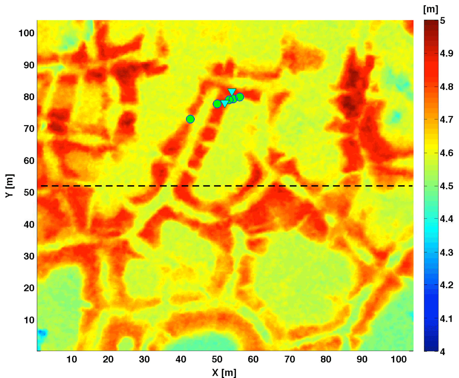
Figure 1The NGEE-Arctic study area A, which was characterized as a low-centered polygon field. The dotted line indicates the transect along which the simulations in this paper are performed to demonstrate the effects of snow redistribution on soil temperature. The locations where snow and temperature sensors are installed within the study site are denoted by triangles and circles, respectively.
2.2 ELMv0 description
The original version of ELM is equivalent to CLM4.5 (Ghimire et al., 2016; Koven et al., 2013; Oleson et al., 2013) and represents vertical energy and water dynamics, including phase change. We developed ELM-3D by expanding on that model to explicitly represent soil lateral energy and hydrological exchanges and fine-resolution snow redistribution. We run ELM-3D here with prescribed plant phenology (called the “satellite phenology” (SP) mode) since our focus is on thermal dynamics of the system, rather than C cycle dynamics.
2.3 Representing two-dimensional and three-dimensional physics
2.3.1 Subsurface hydrology
The flow of water in the unsaturated zone is given by the θ-based Richards equation as
where θ (m3 m−3) is the volumetric soil water content, t (s) is time, q (ms−1) is the Darcy flux, and Q (m−3 of water m−3 of soil s−1) is the volumetric sink of water. The Darcy flux is given by
where k (ms−1) is the hydraulic conductivity, ψ (m) is the soil matric potential, and z (m) is the height above a reference datum. The hydraulic conductivity and soil matric potential are nonlinear functions of volumetric soil moisture. ELMv0 uses the modified form of the Richards equation of Zeng and Decker (2009) that computes the Darcy flux as
where C is a constant hydraulic potential above the water table, z∇, given as
where ψE (m) is the equilibrium soil matric potential, ψsat (m) is the saturated soil matric potential, θE (m3 m−3) is the volumetric soil water content at equilibrium soil matric potential, θsat (m3 m−3) is the volumetric soil water content at saturation, z∇ (m) is the height of water table above the reference datum, and B (−) is a fitting parameter for soil water characteristic curves. Substituting Eqs. (3) and (4) into Eq. (1) yields the equation for the vertical transport of water in ELMv0:
A finite volume spatial discretization and implicit temporal discretization with Taylor series expansion leads to a tridiagonal system of equations. We extended this 1-D (one-dimensional) Richards equation to a 3-D (three-dimensional) representation integrated in ELM-3D, which is presented next.
We use a cell-centered finite volume discretization to decompose the spatial domain into N non-overlapping control volumes, Ωn, such that , and Γn represents the boundary of the nth control volume. Applying a finite volume integral to Eq. (1) and the divergence theorem yields
The spatially discretized equation for the nth grid cell that has Vn volume and n′ neighbors is given by
For the sake of simplicity in presenting the discretized equation, we assume the 3-D grid is a Cartesian grid, with each grid cell having a thickness of Δx, Δy, and Δz in the x, y, and z directions, respectively. Using an implicit time integral, the 3-D discretized equation at time t+1 for a ( control volume is given as
where qx, qy, and qz are the Darcy flux in the x, y, and z directions, respectively, and is the change in volumetric soil liquid water in time, Δt. Using the same approach as Oleson et al. (2013), the Darcy flux in all three directions is linearized about θ using Taylor series expansion. The linearized Darcy flux in the x direction at the ( interface is a function of and :
The linearized Darcy fluxes in the y and z directions are computed similarly. Substituting Eq. (9) in Eq. (8) results in a banded matrix of the form
where α, β, and γ are subdiagonal entries; η, μ, and ϕ are superdiagonal entries; ζ is a diagonal entry of the banded matrix and is given by
The column vector φ is given by
The coefficients of Eq. (10) described in Eqs. (11)–(18) are for an internal grid cell with six neighbors. The coefficients for the top and bottom grid cells are modified for infiltration and interaction with the unconfined aquifer in the same manner as Oleson et al. (2013). Similarly, the coefficients for the grid cells on the lateral boundary are modified for a no-flux boundary condition. See Oleson et al. (2013) for details about the computation of hydraulic properties and derivative of the Darcy flux with respect to soil liquid water content.
2.3.2 Subsurface thermal
ELMv0 solves a tightly coupled system of equations for soil, snow, and standing water temperature (Oleson et al., 2013). The model solves the transient conservation of energy:
where c is the volumetric heat capacity (J m−3 K−1), F is the heat flux (W m−2), and t is time (s). The heat conduction flux is given by
where λ is thermal conductivity (W m−1 K−1) and T is temperature (K). Applying a finite volume integral to Eq. (20) and divergence theorem yields
The spatially discretized equation for a nth grid cell that has Vn volume and n′ neighbors is given by
Similar to the approach taken in Sect. 2.3.1, ELM-3D assumes a 3-D Cartesian grid, with each grid cell having a thickness of Δx, Δy, and Δz in the x, y, and z directions, respectively. Temporal integration of Eq. (22) is carried out using the Crank–Nicholson method that uses a linear combination of fluxes evaluated at time t and t+1:
where ω is the weight in the Crank–Nicholson method and is set to 0.5 in this study. Substituting a discretized form of heat flux using Eq. (20) in Eq. (23) results in a banded matrix of the form
where α, β, and γ are subdiagonal entries; η, μ, and ϕ are superdiagonal entries; ζ is a diagonal entry of the banded matrix and is given by
The column vector φ is given by
The coefficients of Eq. (24) described in Eqs. (25)–(32) are for an internal grid cell with six neighbors. The coefficients for the top grid cells are modified for the presence of snow and/or standing water. A no-flux boundary condition was applied on the bottom grid cells; thus no geothermal flux was accounted for in this study. The coefficients for the grid cells on the lateral boundary are modified for a no-flux boundary condition. ELM handles ice–liquid phase transitions by first predicting temperatures at the end of a time step and then updating temperatures after accounting for deficits or excesses of energy during melting or freezing. See Oleson et al. (2013) for details about the computation of thermal properties and phase transition.
2.3.3 PETSc numerical solution
ELMv0, which considers flow only in the vertical direction, solves a tridiagonal and banded tridiagonal system of equations for water and energy transport, respectively. In ELM-3D, accounting for lateral flow in the subsurface results in a sparse linear system, Eqs. (10) and (24), where the sparsity pattern of the linear system depends on grid cell connectivity. In this work, we use the PETSc (Portable, Extensible Toolkit for Scientific Computing) library (Balay et al., 2016) developed at the Argonne National Laboratory to solve the sparse linear systems. PETSc provides object-oriented data structures and solvers for scalable scientific computation on parallel supercomputers. A description of the numerical tests that were conducted to ensure that the lateral coupling of hydrologic and thermal processes was correctly implemented is presented in the Supplement (Figs. S1 and S2)
2.4 Snow model and redistribution
The snow model in ELM-3D is the same as that in the default ELMv0 and CLM4.5 (Anderson, 1976; Dai and Zeng, 1997; Jordan, 1991), except for the inclusion of snow redistribution (SR). The snow model allows for a dynamic snow depth and up to five snow layers, and explicitly solves the vertically resolved mass and energy budgets. Snow aging, compaction, and phase change are all represented in the snow model formulation. Additionally, the snow model accounts for the influence of aerosols (including black and organic carbon and mineral dust) on snow radiative transfer (Oleson et al., 2013). ELMv0 uses the methodology of Swenson and Lawrence (2012) to compute fractional snow cover area, which is appropriate for ESM-scale grid cells (∼ 100 km × 100 km). Since the grid cell resolution in this work is sub-meter, we modified the fractional cover to be either 1 (when snow was present) or 0 (when snow was absent).
Two main drivers of SR include topography and surface wind (Warscher et al., 2013); previous SR models include mechanistically based (Bartelt and Lehning, 2002; Liston and Elder, 2006) and empirically based (Frey and Holzmann, 2015; Helfricht et al., 2012) approaches. To mimic the effects of wind, we used a conceptual model to simulate SR over the fine-resolution topography of our site by instantaneously re-distributing the incoming snow flux such that lower elevation areas (polygon center) receive snow before higher elevation areas (polygon rims). This relatively simple and parsimonious approach is reasonable given the observed snow depth heterogeneity, as described below, and small spatial extent of our domain.
2.5 System characterization
Hydrologic and thermal properties differ by depth and landscape type. We used the horizontal distribution of organic matter content from Wainwright et al. (2015) to infer soil hydrologic and thermal properties following the default representations in ELM. Vegetation cover was classified as arctic shrubs in polygon centers and arctic grasses in polygon rims. The default representation of the plant wilting factor assigns a value of zero for a given soil layer when its temperature falls below a threshold (Tthreshold) of −2 ∘C. This default value leads to overly large predicted latent and sensible heat fluxes during winter, compared to nearby eddy covariance measurements. We modified Tthreshold to be 0 ∘C in this study, resulting in improved predicted wintertime latent heat fluxes compared to the default version of the model (Fig. S3). Although biases compared to the observations remain, particularly for sensible heat fluxes in the spring, the improvement is substantial and, given the observational uncertainties, we believe sufficient to justify our use of the model for investigations of the role of snow heterogeneity in this polygonal tundra system.
2.6 Simulation setup, climate forcing, and analyses
Because of computational constraints, we investigated the role of snow redistribution and physics representation using a two-dimensional transect through site A (Fig. 1). The transect was 104 m long and 45 m deep and was discretized horizontally with a grid spacing of 0.25 m and an exponentially varying layer thickness in the vertical with 30 soil layers. The transect does not align with the sensor locations because our objective was not to validate the model for a few grid cells, but to focus on relative differences between predictions for rims and centers of a polygon field. No flow conditions for mass and energy were imposed on the east, west, and bottom boundaries of the domain. Temporal discretization of 30 min was used in the simulations. All simulations were performed in the satellite phenology (SP) mode; i.e., Leaf Area Index (LAI) was prescribed from MODIS observations.
Simulations were run for 10 years using long-term climate data gathered at the Barrow Alaska Observatory site (https://www.esrl.noaa.gov/gmd/obop/brw/) managed by the Global Monitoring Division of NOAA's Earth System Research Laboratory (Mefford et al., 1996). The missing precipitation time series was gap-filled using daily precipitation at the Barrow Regional Airport available from the Global Historical Climatology Network (http://www1.ncdc.noaa.gov/pub/data/ghcn/daily). We tested the model by comparing predictions to high-frequency observations of snow depth and vertically resolved soil temperature for September 2012–September 2013. Temperature observations were taken at discrete locations in a polygon center and rim (Fig. 1), and they were combined to analyze comparable landscape positions in the simulations (Fig. 2).
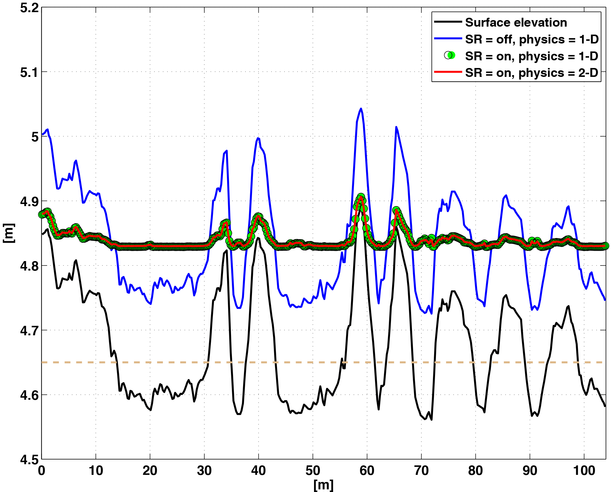
Figure 2Simulated average winter snow surface elevation across the transect for three scenarios: (1) snow redistribution (SR) turned off and 1-D subsurface physics, (2) snow redistribution turned on and 1-D subsurface physics, and (3) snow redistribution turned on and 2-D subsurface physics. Surface elevation of the transect is shown by the solid black line. The dashed line indicates the boundary for comparison to observations in relatively lower (centers) and relatively higher (rims) topographical positions.
After testing, the model was used to investigate the effects of snow redistribution and 2-D subsurface hydrologic and thermal physics by analyzing three scenarios: (1) no snow redistribution and 1-D physics; (2) snow redistribution and 1-D physics; and (3) snow redistribution and 2-D physics. Between these scenarios, we compared vertically resolved soil temperature and liquid saturation, active layer depth, and mean and spatial variation of latent and sensible heat fluxes across the 10 years of simulations. For each soil column, the simulated soil temperature was interpolated vertically, and the active layer depth was estimated as the maximum depth that had above-freezing soil temperature.
3.1 Snow depth
In the absence of SR, predicted snow depth exactly follows the topography. With SR, a much smaller dependence of winter average snow depth on topography is predicted (Fig. 2). Further, for the winter average, there are very small differences in snow depth between simulations with SR and 1-D or 2-D subsurface physics representations. Compared to observations, considering SR led to (1) a factor of ∼ 2 improvement in snow depth bias for the polygon center; (2) modest increase and decrease in average bias on the rims for September through February and March through June, respectively; and (3) a dramatic improvement in bias of the difference in snow depth between the polygon centers and rims (Fig. 3). There was no discernible difference in snow depth bias between the 1-D and 2-D physics (Table 1), although the predicted subsurface temperature fields were different, as shown below.
Table 1Bias, root mean square error (RMSE), and correlation (R2) between modeled and observed snow depth at polygon center and rim, and the difference between center and rim for 2013 for three cases: snow redistribution (SR) off and 1-D physics, SR on and 1-D physics, and SR on and 2-D physics.
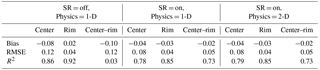
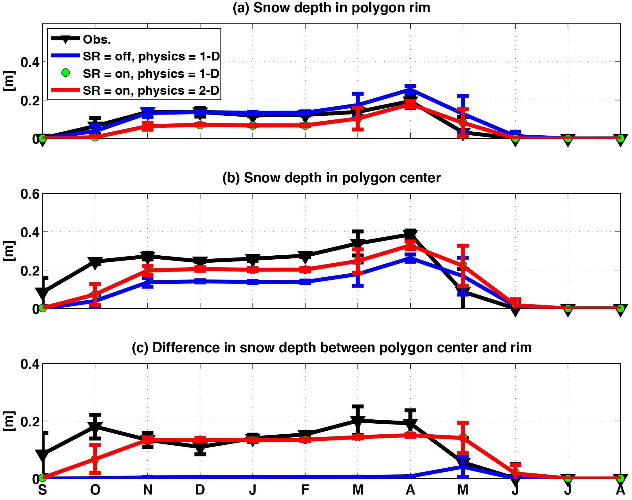
Figure 3Monthly mean comparison of observation and simulated snow depth (a) in polygon rim and (b) in polygon center; (c) difference between polygon center and rim for 2013.
The temporal variation of the mean snow depth (Fig. 4a) and its spatial standard deviation (Fig. 4b) also differed based on whether SR was considered, but it was not affected by considering 2-D thermal or hydrologic physics. With SR, the snow depth coefficient of variation (Fig. 4c) was about 0.5 from December through the beginning of the snowmelt period, indicating relatively large spatial heterogeneity. Simulated snow depths for the three simulation scenarios are included in the Supplement (4).
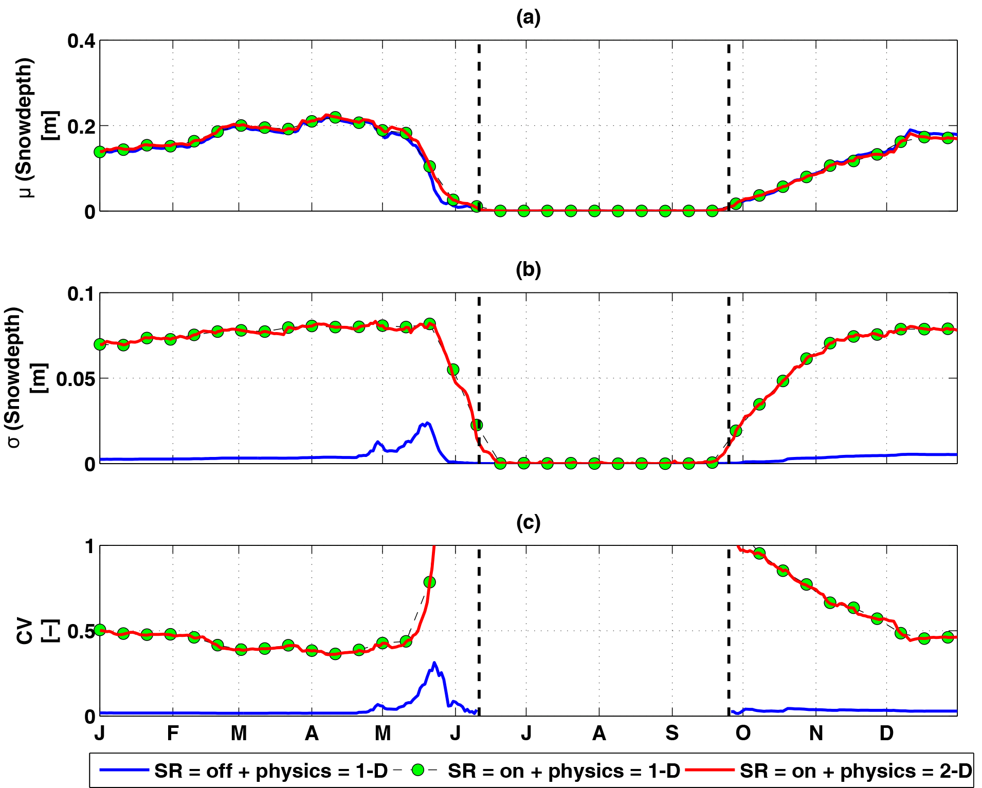
Figure 4(a) Mean, (b) standard deviation, and (c) coefficient of variation of simulated snow depth across the entire domain for 1-D and 2-D subsurface physics.
3.2 Soil temperature and active layer depth
Broadly, ELM-3D accurately predicted the polygon center soil temperature at depth intervals corresponding to the temperature probes (0–20, 20–50, 50–75, and 75–100 cm; Fig. 5a). Recall that the observed temperatures for the polygon center and rims were taken at single points in site A (Fig. 1), while the predicted temperatures were calculated as averages across the transect for each of the two landscape position types. The model was able to simulate early freeze-up of the soil column under the rims as compared to centers in November 2012 because of differences in accumulated snowpack. The transition to thawed soil in the 0–20 cm depth interval in early June 2013 and the subsequent temperature dynamics over the summer were very well captured by ELM-3D. Minimum temperatures during the winter were also accurately predicted, although the temperatures in the deepest layer (75–100 cm) were overestimated by ∼ 3 ∘C in March. For figure clarity we did not indicate the standard deviation of the observations but provide that information in the Supplement (Figs. S5–S8).
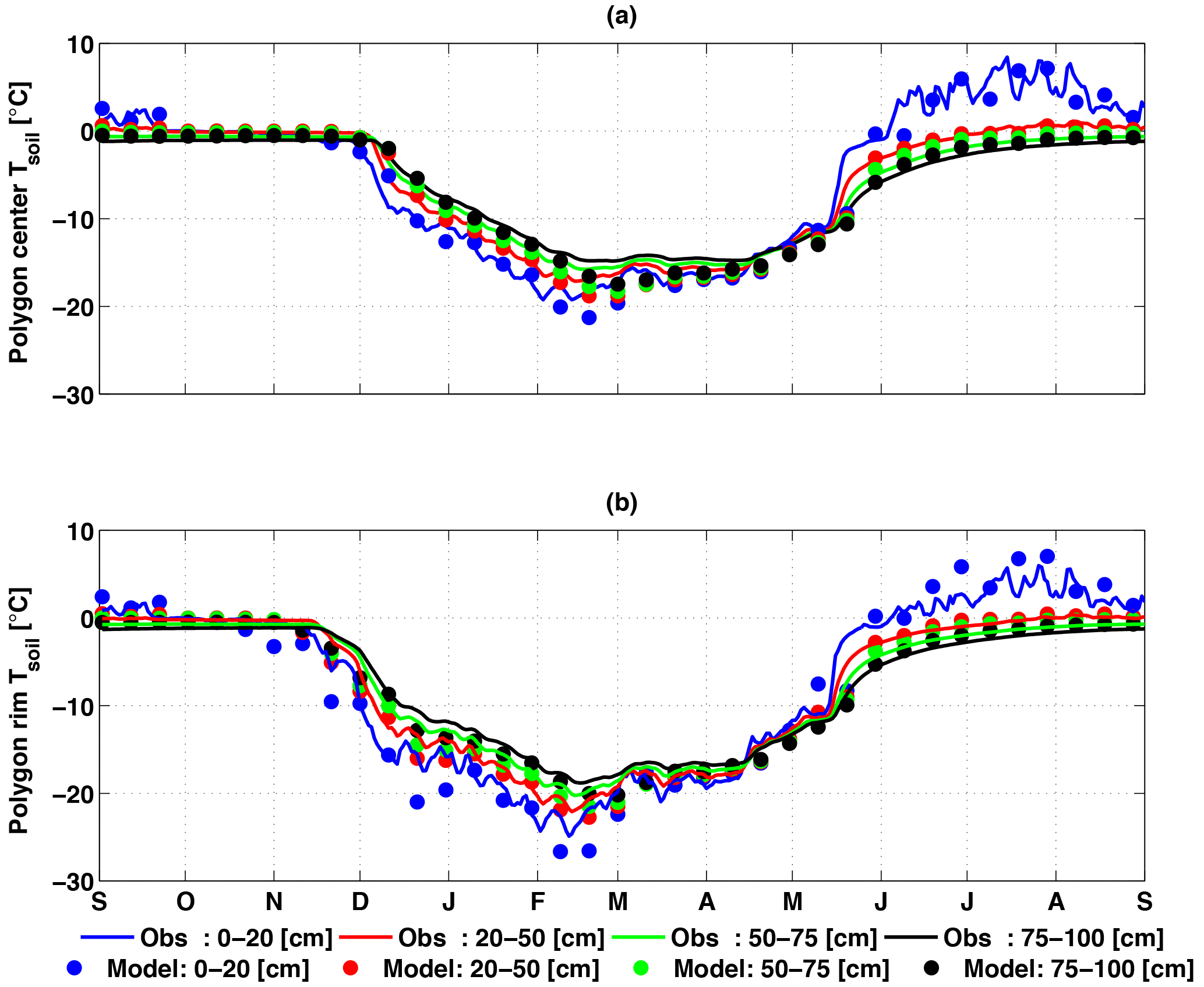
Figure 5Comparison of soil temperature observations and predictions in polygon centers (a) and rims (b). Simulation was performed with snow redistribution on and 2-D subsurface physics, between September 2012 and September 2013. Simulation results are shown at an interval of 10 days, while observations are shown at a daily interval.
Similarly, the soil temperatures were accurately predicted in the polygon rims (Fig. 5b). The largest discrepancies between measured and predicted soil temperatures were in the shallowest layer (0–25 cm), where the predictions were up to a few ∘C cooler than some of the observations between December 2012 and March 2013. In the polygon center, a thicker snowpack acts as a heat insulator and keeps soil temperature higher in winter as compared to the polygon rims.
Three recent studies have used other mechanistic models to simulate soil temperature fields at this site and achieved comparably good comparisons with observations (Kumar et al., 2016 applied a 3-D version of PFLOTRAN; Atchley et al., 2015 and Harp et al., 2016 applied a 1-D version of the Arctic Terrestrial Simulator – ATS). However, those models used measured soil temperatures near the surface as the top boundary condition. In contrast, the top boundary condition in this work is the climate forcing (air temperature, wind, solar radiation, humidity, precipitation), and the ground heat flux is predicted based on ELM's vegetation and surface energy dynamics. We note that no parameter calibration was done in this work or that of Kumar et al. (2016), while the ATS parameterizations were calibrated to match the soil temperature profile.
Snow redistribution impacts spatial variability of soil temperature throughout the soil column. Absence of SR results in no significant spatial variability of soil temperature (Fig. 6a). Inclusion of SR on the surface modifies the amount of energy exchanged between the snow and the top soil layer, thereby creating spatial variability in the temperature of the top soil, which propagates down into the soil column (Fig. 6b). With SR, energy dissipation in the lateral direction reduces the penetration depth of the soil temperature spatial variance (compare Fig. 6c and b).
Table 2Bias, root mean square error (RMSE), and correlation (R2) between modeled and observed soil temperature at polygon center and rim at multiple soil depth for 2013 for three cases: snow redistribution (SR) off and 1-D physics, SR on and 1-D physics, and SR on and 2-D physics.
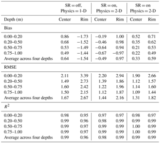
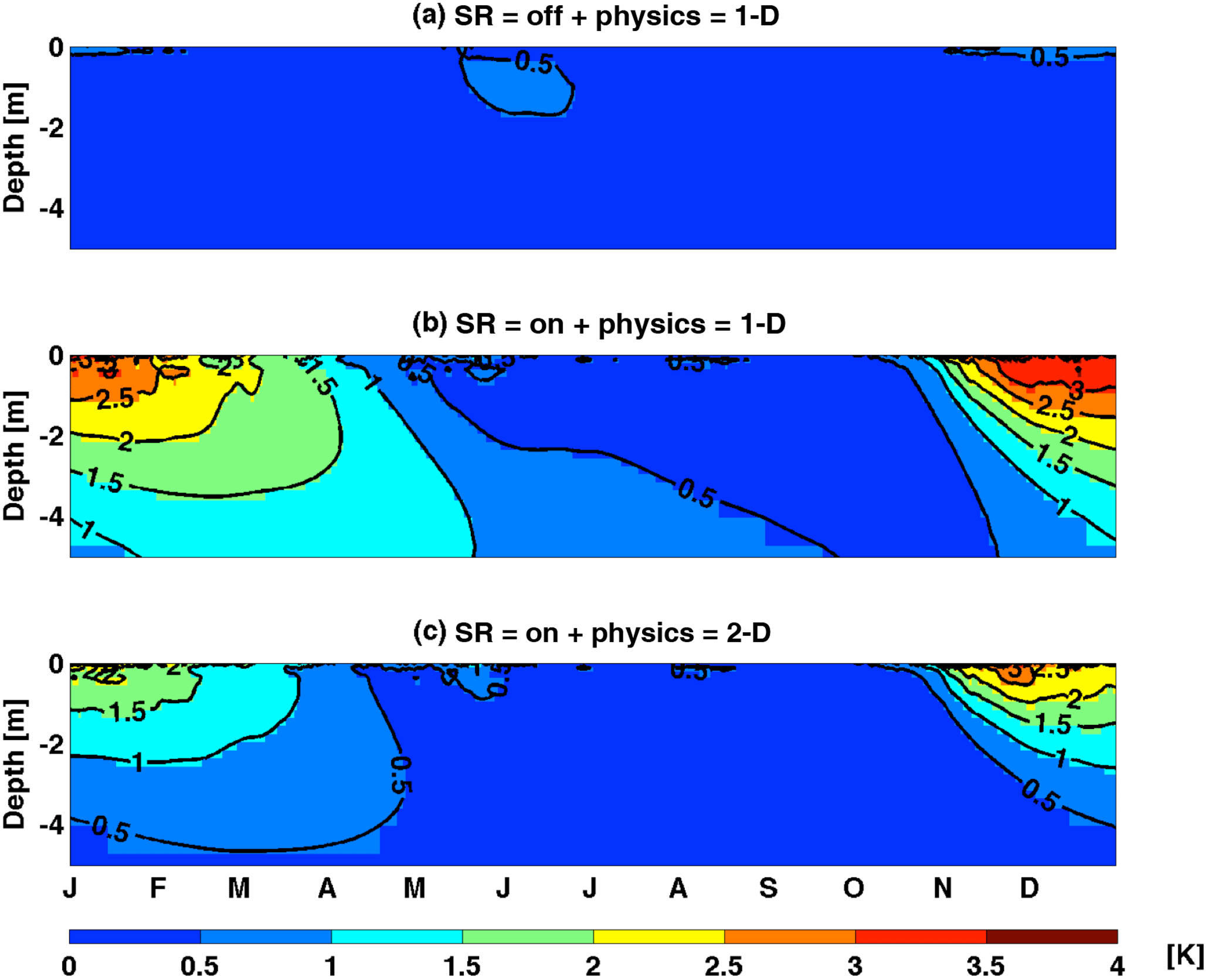
Figure 6Simulated daily spatial standard deviation for each soil layer averaged across 10 years of near-surface soil temperature for the simulation performed with snow redistribution turned off and 1-D subsurface physics (a); snow redistribution turned on and 1-D subsurface physics (b); and snow redistribution turned on and 2-D subsurface physics (c).
With 1-D physics, the average spatial and temporal difference of the active layer depth (ALD) between simulations with and without SR was 1.7 cm (Fig. 7a), and the absolute difference was 6.5 cm. As described above, we diagnosed the ALD to be the maximum soil depth during the summer at which vertically interpolated soil temperature is 0 ∘C. On average, the rims had ∼ 10 cm shallower ALD with (blue line) than without (green line) SR, consistent with the loss of insulation from SR on the rims during the winter. In the centers (e.g., at location 42–55 m), the thaw depth was deeper by ∼ 5 cm with SR because of the higher snow depth there from SR. The effect of SR on the ALD was largest on the rims because, compared to centers, they (1) on average lost more snow with SR and (2) are more thermally conductive. Since rims are therefore colder at the time of snowmelt with SR, the ground heat flux during the subsequent summer was unable to thaw the soil column as deeply as when SR is ignored. For comparison, Atchley et al. (2015) found in their sensitivity analysis using the 1-D version of ATS that SR resulted in deeper thaw depths in both polygon centers (by ∼ 3 cm) and rims (∼ 0.3 cm). Thus, their results for polygon centers are consistent in sign but lower in magnitude than ours, but opposite in sign for the rims.
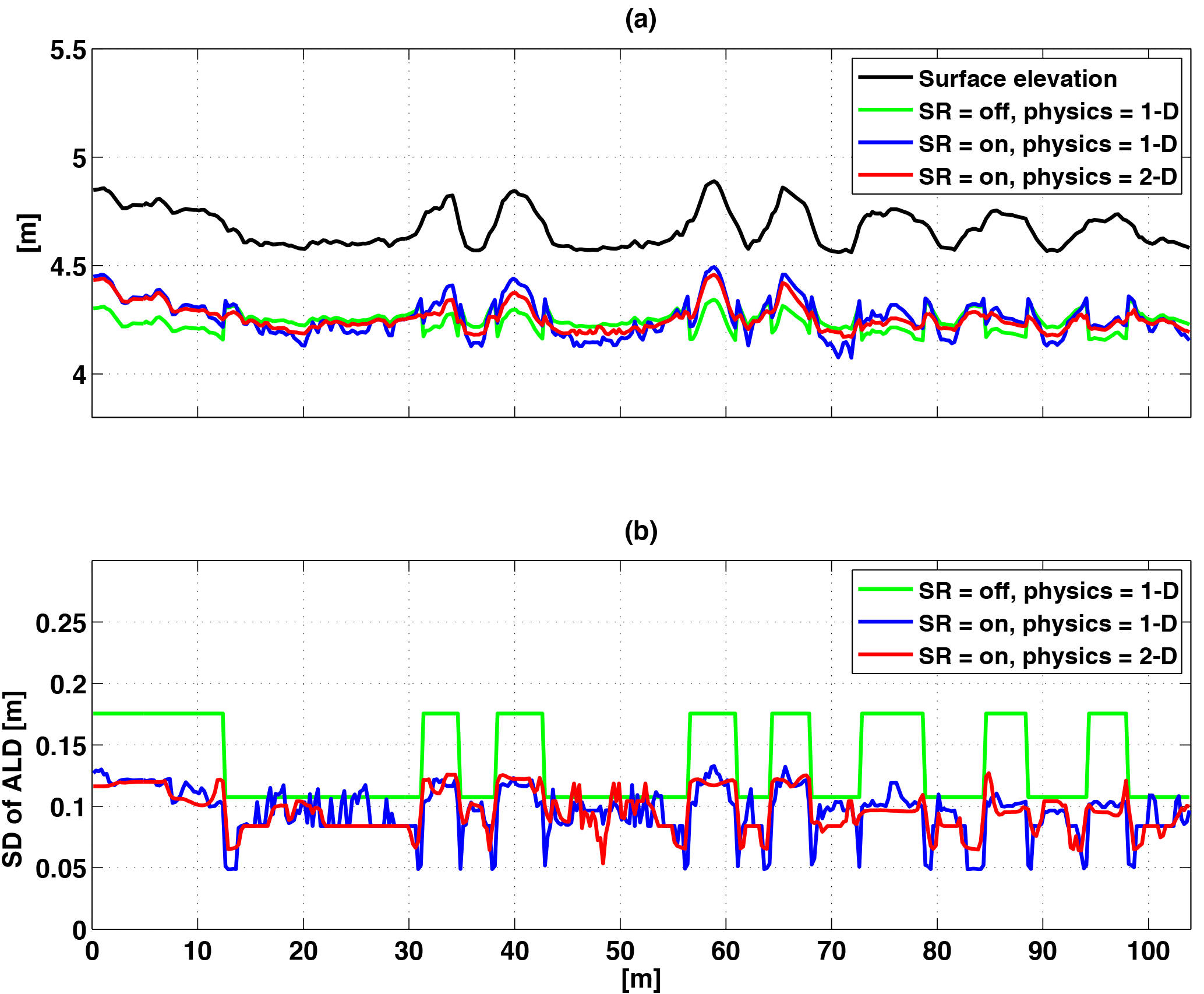
Figure 7Temporal mean of the bottom of the active layer (a) and standard deviation of the active layer depth (b) over the 10-year period across the modeling domain.
Across 10 years of simulation, the interannual variability (IAV) in ALD varied substantially between the three scenarios (Fig. 7b). As expected, for the 1-D physics without SR scenario (green line), the IAV in ALD was determined by a landscape position because of differences in soil and vegetation parameters. With SR and 1-D physics, the model shows largest differences over the rims, again highlighting the relatively larger effects of SR on the rim soil temperatures.
The effect of 1-D versus 2-D physics on the ALD across the transect was modest (mean absolute difference ∼ 3 cm). Generally, because 2-D physics allows for lateral energy diffusion, the horizontal variation of ALD was slightly lower (i.e., the red line is smoother than the blue line; Fig. 7a) than with 1-D physics. This difference was also reflected in the thaw depth IAV across the transect, where 2-D physics led to a smoother lateral profile of interannual variability than with 1-D physics.
The impact of physics formulation (i.e., 1-D or 2-D) alone was investigated by analyzing differences between soil temperature profiles over time for polygon rims and centers in simulations with snow redistribution. Inclusion of 2-D subsurface physics resulted in soil temperatures with depth and time that were lower in the polygon rims (Fig. 8a) and higher in polygon centers (Fig. 8b). Using the simulations from the scenario with SR and 2-D physics, we evaluated the extent to which soils under rims and centers can be separately considered as relatively homogeneous single column systems by evaluating the soil temperature standard deviation as a function of depth and time (Fig. 9). During winter, both polygon rims and centers were predicted to have soil temperature spatial variability > 1 ∘C up to a depth of ∼ 2 m. The soil temperature spatial variability in winter due to snow redistribution was dissipated over the summer. During the summer, polygon centers were relatively more homogeneous vertically compared to polygon rims.
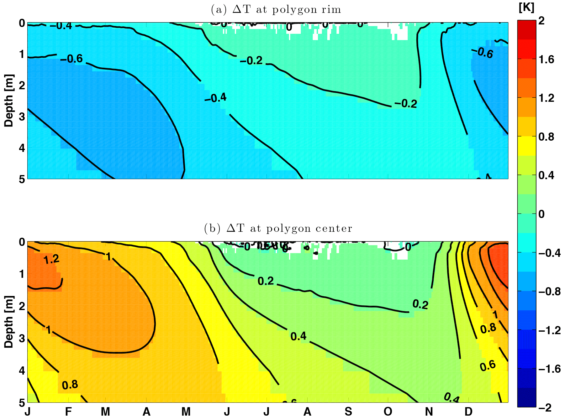
Figure 8Time series of spatial mean soil temperature differences between “SR = on + physics = 1-D” and “SR = on + physics = 2-D” at polygon rim (a) and polygon center (b).
3.3 Surface energy budget
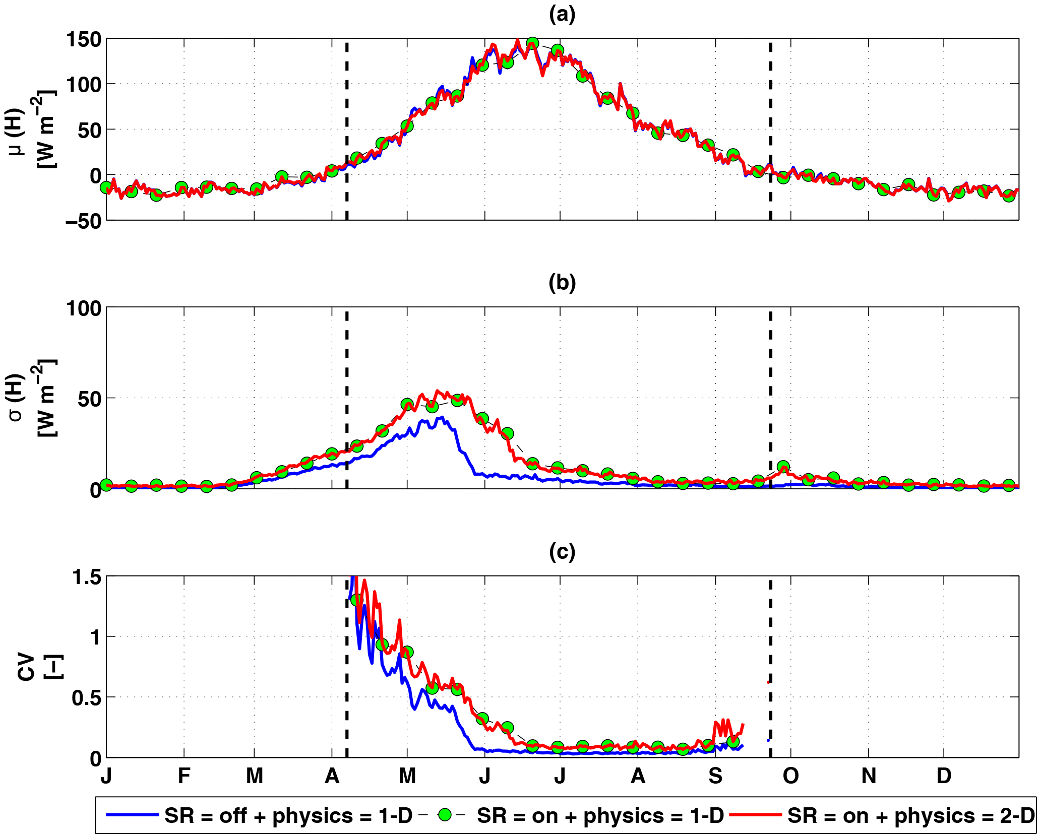
Predicted monthly mean and spatial mean (μ) surface latent heat fluxes across the transect were very similar between the three scenarios (Fig. 10a), with a growing seasonal mean difference of < 1.0 W m−2. However, the spatial variability (SV =σ; Fig. 10b) and coefficient of variation (CV ; Fig. 10c) of latent heat fluxes were different between the scenarios with SR (1-D and 2-D physics) and without SR. With SR, the latent heat flux spatial standard deviation peaked after snowmelt and declined until the fall when snow began, from about ∼ 100 to 10 % of the mean. This relatively larger spatial variation in latent heat flux occurred because of large spatial heterogeneity in near-surface soil moisture in the beginning of summer, indicating a residual effect of SR from the previous winter.
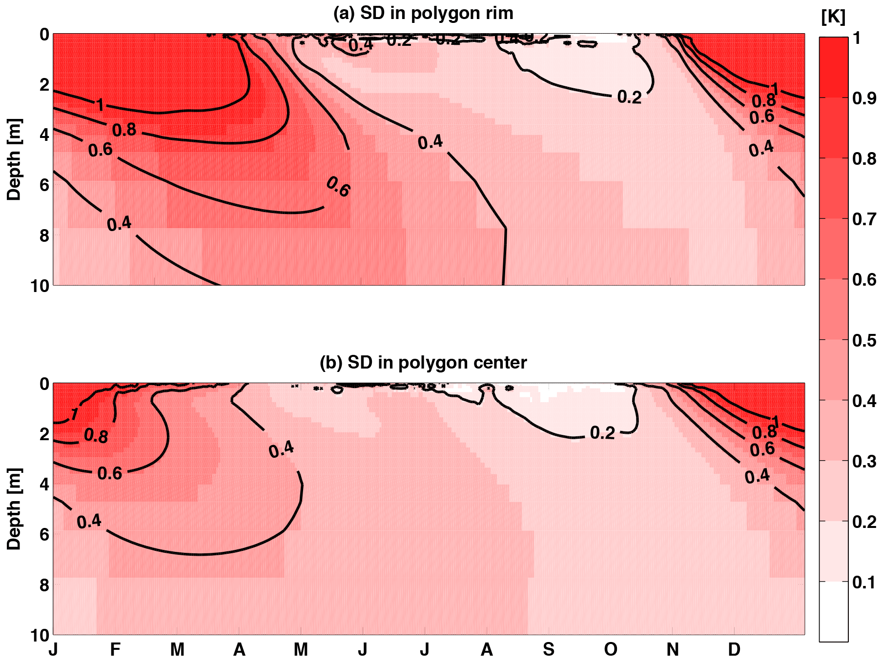
Figure 9Time series of soil temperature spatial standard deviation for “SR = on + physics = 2-D” at polygon rim (a) and polygon center (b).

Figure 10Latent heat flux interannual (a) mean, (b) standard deviation, and (c) coefficient of variation across the site A transect.
The predicted temporal monthly mean and spatial mean surface sensible heat fluxes across the transect were also similar between the three scenarios (Fig. 11a), with a growing season mean absolute difference of < 3.5 W m−2. Also, the sensible heat flux spatial variability differences occurred earlier than snowmelt, in contrast to the latent heat flux. Both the standard deviation and CV of the sensible heat fluxes were larger than those of the latent heat fluxes, with early season standard deviations of ∼ 50 W m−2 (Fig. 11b) and CVs of ∼ 1.5 (Fig. 11c). As for the latent heat fluxes, the differences in standard deviation and CV of sensible heat fluxes were small between the 1-D and 2-D scenarios with SR, arguing that the subsurface lateral energy exchanges associated with the 2-D physics did not propagate to the mean surface heat fluxes. However, as for the latent heat flux, there was a relatively large difference in spatial variation between the scenarios with and without SR (e.g., of about 25 W m−2 in May; Fig. 10b).
3.4 Soil moisture
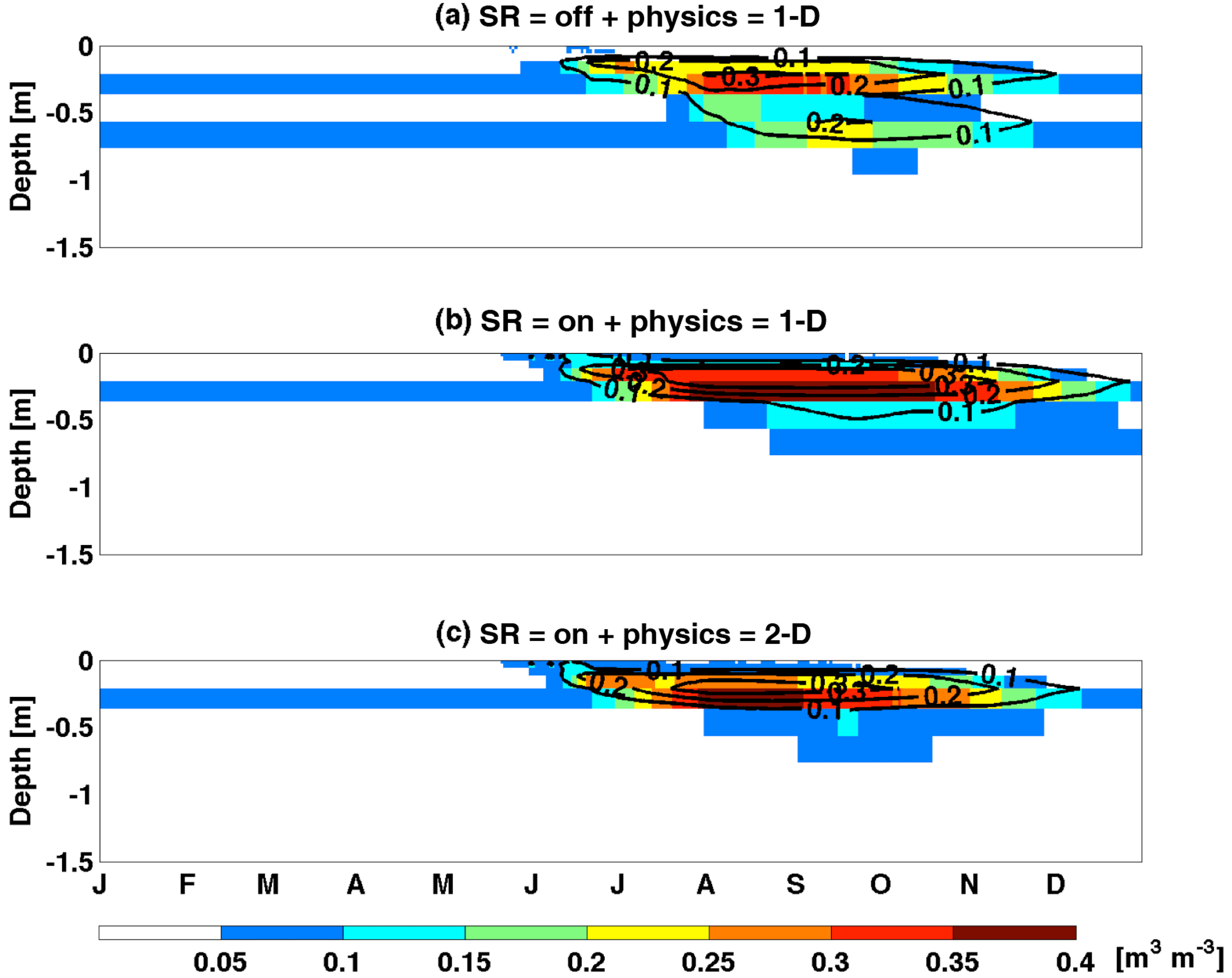
Neither SR nor 2-D lateral physics affected the spatial mean moisture across time (not shown). However, spatial heterogeneity of predicted soil moisture content differed substantially between scenarios during the snow-free period (Fig. 12). For the 1-D simulations, the effect of SR was to increase growing season soil moisture spatial heterogeneity by factors of 5.2 and 1.6 for 0–10 and 10–65 cm depth intervals, respectively (compare Fig. 12a and b). Compared to 1-D physics, simulating 2-D thermal and hydrologic physics led to an overall reduction in soil moisture spatial heterogeneity by factors of 0.8 and 0.7 for 0–10 and 10–65 cm depth intervals, respectively (compare Fig. 12b and c). Thus, with respect to dynamic spatial mean soil moisture, SR effects dominated those associated with lateral subsurface water movement.
3.5 Caveats and future work
The good agreement between ELM-3D predictions and soil temperature observations demonstrates the model's capabilities to represent this very spatially heterogeneous and complex system. However, several caveats to our conclusions remain due to uncertainties in model parameterizations, model structure, and climate forcing data.
ELMv0, a one-dimensional model, is embarrassingly parallel with no cross-processor communication. The current implementation of the three-dimensional solver in ELM-3D only supports serial computing. Support of parallel computing will be included in a future version of the model. Because of computational constraints, we applied a 2-D transect domain to the site, instead of a full 3-D domain. We are working to improve the computational efficiency of the model, which will facilitate a thorough analysis of the effects of 3-D subsurface energy and water fluxes. A related issue is our simplified treatment of surface water flows. A thorough analysis of the effects of surface water redistribution would require integration of a 2-D surface thermal flow model in a 3-D domain, which is another goal for our future work. However, we note that the good agreement using the 2-D model domain supports the idea that a two-dimensional simplification may be appropriate for this system. The expected geomorphological changes in these systems over the coming decades (e.g., Liljedahl et al., 2016), which will certainly affect soil temperature and moisture, are not currently represented in ELM, although incorporation of these processes is a long-term development goal.
The current representation of vegetation in ELM-3D for these polygonal tundra systems is oversimplified. For example, non-vascular plants (mosses and lichens) are not explicitly represented in the model, but can be responsible for a majority of evaporative losses (Miller et al., 1976) and are strongly influenced by near-surface hydrologic conditions (Williams and Flanagan, 1996). Our use of the satellite phenology mode, which imposes transient LAI profiles on each plant functional type in the domain, ignores the likely influence of nutrient constraints (Zhu et al., 2016) on photosynthesis and therefore the surface energy budget. Other model simplifications, e.g., the simplified treatment of radiation competition, may also be important, especially as simulations are extended over periods where vegetation change may occur (e.g., Grant et al., 2015).
Development of subgrid parameterizations to parsimoniously capture fine-scale processes will be pursued in the future. For example, a two-tile approach to represent hydrologic and thermal processes in coupled polygon rims and centers with snow redistribution should be evaluated. Inclusion of lateral subsurface processes has a greater impact on predicted subgrid variability than on spatially averaged states. Thus, one possible extension of the current model would be to explicitly include an equation for the temporal evolution of subgrid variability using the approach of Montaldo and Albertson (2003). The use of reduced-order models (e.g., Pau et al., 2014; Liu et al., 2017) is an alternate approach to estimate fine-scale hydrologic and thermal states from a coarse resolution representation. Additionally, lateral subsurface processes can be included in the land surface model via a range of numerical discretization approaches of varying complexity, e.g., adding lateral water and energy fluxes as source–sink terms in the existing 1-D model, implementing an operator split approach to solve vertical and lateral processes in a non-iterative approach, or solving a fully coupled 3-D model. Trade-offs between approaches that represent lateral processes and computational costs need to be carefully studied before developing quasi or fully three-dimensional land surface models. While the present study focused on application and validation of ELM-3D at fine-scale, future work will focus on regional-scale applications using comprehensive datasets and the Distributed Model Intercomparison Project Phase 2 modeling protocol (Smith et al., 2012). Although we found no significant effect of topography and SR on the 100 m × 100 m grid-averaged exchanges with the atmosphere, future work needs to analyze intermediate-scale (e.g., 100 m–10 km) topographical variation and the potential effects on biogeochemical and plant processes and surface exchanges.
In a polygonal tundra landscape, we analyzed effects of microtopographical surface heterogeneity and lateral subsurface transport on soil temperature, soil moisture, and surface energy exchanges. Starting from the climate-scale land model ELMv0, we incorporated in ELM-3D numerical representations of subsurface water and energy lateral transport that are solved using PETSc. A simple method for redistributing incoming snow along the microtopographic transect was also integrated in the model.
Over the observational record, ELM-3D with snow redistribution and lateral heat and hydrological fluxes accurately predicted snow depth and soil temperature vertical profiles in the polygon rims and centers (overall bias, RMSE, and R2 of 0.59 ∘C, 1.82 ∘C, and 0.99, respectively). In the rims, the transition to thawed soil in spring, summer temperature dynamics, and minimum temperatures during the winter were all accurately predicted. In the centers, a ∼ 2 ∘C warm bias in April in the 75–100 cm soil layer was predicted, although this bias disappeared during snowmelt.
The spatial heterogeneity of snow depth during the winter due to snow redistribution generated surface soil temperature heterogeneity that propagated into the soil over time. The temporal and spatial variation of snow depth was affected by snow redistribution, but not by lateral thermal and hydrologic transport. Both snow redistribution and lateral thermal fluxes affected spatial variability of soil temperatures. Energy dissipation in the lateral direction reduced the depth to which soil temperature variance penetrated. Snow redistribution led to ∼ 10 cm shallower active layer depths under the polygon rims because of the residual effect of reduced insulation during the winter. In contrast, snow redistribution led to ∼ 5 cm deeper maximum thaw depth under the polygon centers. The effect of lateral energy fluxes on active layer depths was ∼ 3 cm. Compared to 1-D physics, the 2-D subsurface physics led to lower (higher) soil temperatures with depth and time in the polygon rims (centers). The larger than 1 ∘C wintertime spatial temperature variability down to ∼ 2 m depth in rims and centers indicates the uncertainty associated with considering rims and centers as separate 1-D columns. During the summer, polygon center temperatures were relatively more vertically homogeneous than temperatures in the rims.
The monthly mean and spatial mean predicted latent and sensible heat fluxes were unaffected by snow redistribution and lateral heat and hydrological fluxes. However, snow redistribution led to spatial heterogeneity in surface energy fluxes and soil moisture during the summer. Excluding lateral subsurface hydrologic and thermal processes led to an overprediction of spatial variability in soil moisture and soil temperature because subsurface gradients were artificially prevented from laterally dissipating over time. Snow redistribution effects on soil moisture heterogeneity were larger than those associated with lateral thermal fluxes.
Overall, our analysis demonstrates the potential and value of explicitly representing snow redistribution and lateral subsurface hydrologic and thermal dynamics in polygonal ground systems and quantifies the effects of these processes on the resulting system states and surface energy exchanges with the atmosphere. The integration of a 3-D subsurface model in the E3SM Land Model also allows for a wide range of analyses heretofore impossible in an Earth System Model context.
The ELM-3D v1.0 code and data used in study are publicly available at https://bitbucket.org/gbisht/lateral-subsurface-model (commit hash 2a31e42d911c1d7539230848d3479533d7605912) and https://bitbucket.org/gbisht/notes-for-gmd-2017-71.
The supplement related to this article is available online at: https://doi.org/10.5194/gmd-11-61-2018-supplement.
The authors declare that they have no conflict of interest.
This research was supported by the Director, Office of Science, Office of
Biological and Environmental Research of the US Department of Energy under
contract no. DE-AC02-05CH11231 as part of the NGEE-Arctic and Energy
Exascale Earth System Model (E3SM) programs.
Edited by: Philippe Peylin
Reviewed by: three anonymous referees
Anderson, E. A.: A point energy and mass balance model of a snow cover, National Weather Service, Silver Spring, MD, 1976.
Atchley, A. L., Painter, S. L., Harp, D. R., Coon, E. T., Wilson, C. J., Liljedahl, A. K., and Romanovsky, V. E.: Using field observations to inform thermal hydrology models of permafrost dynamics with ATS (v0.83), Geosci. Model Dev., 8, 2701–2722, https://doi.org/10.5194/gmd-8-2701-2015, 2015.
Balay, S., Abhyankar, S., Adams, M. F., Brown, J., Brune, P., Buschelman, K., Dalcin, L., Eijkhout, V., Gropp, W. D., Kaushik, D., Knepley, M. G., McInnes, L. C., Rupp, K., Smith, B. F., Zampini, S., Zhang, H., and Zhang, H.: PETSc Users Manual, Argonne National Laboratory, ANL-95/11 – Revision 3.7, 1–241, 2016.
Bartelt, P. and Lehning, M.: A physical SNOWPACK model for the Swiss avalanche warning: Part I: numerical model, Cold Reg. Sci. Technol., 35, 123–145, 2002.
Borner, A. P., Kielland, K., and Walker, M. D.: Effects of Simulated Climate Change on Plant Phenology and Nitrogen Mineralization in Alaskan Arctic Tundra, Arct. Antarct. Alp. Res., 40, 27–38, 2008.
Callaghan, T., Johansson, M., Brown, R., Groisman, P., Labba, N., Radionov, V., Barry, R., Bulygina, O., Essery, R. H., Frolov, D. M., Golubev, V., Grenfell, T., Petrushina, M., Razuvaev, V., Robinson, D., Romanov, P., Shindell, D., Shmakin, A., Sokratov, S., Warren, S., and Yang, D.: The Changing Face of Arctic Snow Cover: A Synthesis of Observed and Projected Changes, AMBIO, 40, 17–31, 2011a.
Callaghan, T., Johansson, M., Brown, R., Groisman, P., Labba, N., Radionov, V., Bradley, R., Blangy, S., Bulygina, O., Christensen, T., Colman, J., Essery, R. H., Forbes, B., Forchhammer, M., Golubev, V., Honrath, R., Juday, G., Meshcherskaya, A., Phoenix, G., Pomeroy, J., Rautio, A., Robinson, D., Schmidt, N., Serreze, M., Shevchenko, V., Shiklomanov, A., Shmakin, A., Sköld, P., Sturm, M., Woo, M.-K., and Wood, E.: Multiple Effects of Changes in Arctic Snow Cover, AMBIO, 40, 32–45, 2011b.
Clark, M. P., Hendrikx, J., Slater, A. G., Kavetski, D., Anderson, B., Cullen, N. J., Kerr, T., Örn Hreinsson, E., and Woods, R. A.: Representing spatial variability of snow water equivalent in hydrologic and land-surface models: A review, Water Resour. Res., 47, W07539, https://doi.org/10.1029/2011WR010745, 2011.
Cox, P. M., Betts, R. A., Jones, C. D., Spall, S. A., and Totterdell, I. J.: Acceleration of global warming due to carbon-cycle feedbacks in a coupled climate model, Nature, 408, 184–187, 2000.
Dai, Y. and Zeng, Q.: A land surface model (IAP94) for climate studies part I: Formulation and validation in off-line experiments, Adv. Atmos. Sci., 14, 433–460, 1997.
Dufresne, J. L., Fairhead, L., Le Treut, H., Berthelot, M., Bopp, L., Ciais, P., Friedlingstein, P., and Monfray, P.: On the magnitude of positive feedback between future climate change and the carbon cycle, Geophys. Res. Lett., 29, 43-41–43-44, 2002.
Engstrom, R., Hope, A., Kwon, H., Stow, D., and Zamolodchikov, D.: Spatial distribution of near surface soil moisture and its relationship to microtopography in the Alaskan Arctic coastal plain, Nord. Hydrol., 36, 219–234, 2005.
Euskirchen, E. S., McGuire, A. D., Chapin, F. S., Yi, S., and Thompson, C. C.: Changes in vegetation in northern Alaska under scenarios of climate change, 2003–2100: implications for climate feedbacks, Ecol. Appl., 19, 1022–1043, 2009.
Frey, S. and Holzmann, H.: A conceptual, distributed snow redistribution model, Hydrol. Earth Syst. Sci., 19, 4517–4530, https://doi.org/10.5194/hess-19-4517-2015, 2015.
Friedlingstein, P., Bopp, L., Ciais, P., Dufresne, J.-L., Fairhead, L., LeTreut, H., Monfray, P., and Orr, J.: Positive feedback between future climate change and the carbon cycle, Geophys. Res. Lett., 28, 1543–1546, 2001.
Friedlingstein, P., Cox, P., Betts, R., Bopp, L., von Bloh, W., Brovkin, V., Cadule, P., Doney, S., Eby, M., Fung, I., Bala, G., John, J., Jones, C., Joos, F., Kato, T., Kawamiya, M., Knorr, W., Lindsay, K., Matthews, H. D., Raddatz, T., Rayner, P., Reick, C., Roeckner, E., Schnitzler, K. G., Schnur, R., Strassmann, K., Weaver, A. J., Yoshikawa, C., and Zeng, N.: Climate–Carbon Cycle Feedback Analysis: Results from the C4MIP Model Intercomparison, J. Climate, 19, 3337–3353, 2006.
Fung, I. Y., Doney, S. C., Lindsay, K., and John, J.: Evolution of carbon sinks in a changing climate, P. Natl. Acad. Sci. USA, 102, 11201–11206, 2005.
Galen, C. and Stanton, M. L.: Responses of Snowbed Plant Species to Changes in Growing-Season Length, Ecology, 76, 1546–1557, 1995.
Ghimire, B., Riley, W. J., Koven, C. D., Mu, M., and Randerson, J. T.: Representing leaf and root physiological traits in CLM improves global carbon and nitrogen cycling predictions, J. Adv. Model. Earth Sy., 8, 598–613, 2016.
Govindasamy, B., Thompson, S., Mirin, A., Wickett, M., Caldeira, K., and Delire, C.: Increase of carbon cycle feedback with climate sensitivity: results from a coupled climate and carbon cycle model, Tellus B, 57, 153–163, https://doi.org/10.1111/j.1600-0889.2005.00135.x, 2011.
Grant, R. F., Humphreys, E. R., and Lafleur, P. M.: Ecosystem CO2 and CH4 exchange in a mixed tundra and a fen within a hydrologically diverse Arctic landscape: 1. Modeling versus measurements, J. Geophys. Res.-Biogeo., 120, 1366–1387, https://doi.org/10.1002/2014JG002888, 2015.
Groendahl, L., Friborg, T., and Soegaard, H.: Temperature and snow-melt controls on interannual variability in carbon exchange in the high Arctic, Theor. Appl. Climatol., 88, 111–125, 2007.
Grogan, P. and Chapin III, F. S.: Arctic Soil Respiration: Effects of Climate and Vegetation Depend on Season, Ecosystems, 2, 451–459, 1999.
Harp, D. R., Atchley, A. L., Painter, S. L., Coon, E. T., Wilson, C. J., Romanovsky, V. E., and Rowland, J. C.: Effect of soil property uncertainties on permafrost thaw projections: a calibration-constrained analysis, The Cryosphere, 10, 341–358, https://doi.org/10.5194/tc-10-341-2016, 2016.
Hartman, M. D., Baron, J. S., Lammers, R. B., Cline, D. W., Band, L. E., Liston, G. E., and Tague, C.: Simulations of snow distribution and hydrology in a mountain basin, Water Resour. Res., 35, 1587–1603, 1999.
Helfricht, K., Schöber, J., Seiser, B., Fischer, A., Stötter, J., and Kuhn, M.: Snow accumulation of a high alpine catchment derived from LiDAR measurements, Adv. Geosci., 32, 31–39, 2012.
Hinkel, K. M., Eisner, W. R., Bockheim, J. G., Nelson, F. E., Peterson, K. M., and Dai, X.: Spatial Extent, Age, and Carbon Stocks in Drained Thaw Lake Basins on the Barrow Peninsula, Alaska, Arct. Antarct. Alp. Res., 35, 291–300, 2003.
Hinkel, K. M., Frohn, R. C., Nelson, F. E., Eisner, W. R., and Beck, R. A.: Morphometric and spatial analysis of thaw lakes and drained thaw lake basins in the western Arctic Coastal Plain, Alaska, Permafrost Periglac., 16, 327–341, 2005.
Hinzman, L. D. and Kane, D. L.: Potential repsonse of an Arctic watershed during a period of global warming, J. Geophys. Res.-Atmos., 97, 2811–2820, 1992.
Holland, M. M. and Bitz, C. M.: Polar amplification of climate change in coupled models, Clim. Dynam., 21, 221–232, 2003.
Jiang, D., Zhang, Y., and Lang, X.: Vegetation feedback under future global warming, Theor. Appl. Climatol., 106, 211–227, 2011.
Jones, C. D., Cox, P. M., Essery, R. L. H., Roberts, D. L., and Woodage, M. J.: Strong carbon cycle feedbacks in a climate model with interactive CO2 and sulphate aerosols, Geophys. Res. Lett., 30, 1479, https://doi.org/10.1029/2003GL016867, 2003.
Jones, H. G.: The ecology of snow-covered systems: a brief overview of nutrient cycling and life in the cold, Hydrol. Process., 13, 2135–2147, 1999.
Jordan, R. E.: One-dimensional temperature model for a snow cover: technical documentation for SNTHERM.89, Cold Regions Research and Engineering Laboratory (U.S.) Engineer Research and Development Center (U.S.), 1991.
Jorgenson, M. T., Shur, Y. L., and Pullman, E. R.: Abrupt increase in permafrost degradation in Arctic Alaska, Geophys. Res. Lett., 33, L02503, https://doi.org/10.1029/2005GL024960, 2006.
Koven, C. D., Riley, W. J., Subin, Z. M., Tang, J. Y., Torn, M. S., Collins, W. D., Bonan, G. B., Lawrence, D. M., and Swenson, S. C.: The effect of vertically resolved soil biogeochemistry and alternate soil C and N models on C dynamics of CLM4, Biogeosciences, 10, 7109–7131, https://doi.org/10.5194/bg-10-7109-2013, 2013.
Koven, C. D., Ringeval, B., Friedlingstein, P., Ciais, P., Cadule, P., Khvorostyanov, D., Krinner, G., and Tarnocai, C.: Permafrost carbon-climate feedbacks accelerate global warming, P. Natl. Acad. Sci. USA, 108, 14769–14774, 2011.
Koven, C. D., Lawrence, D. M., and Riley, W. J.: Permafrost carbon-climate feedback is sensitive to deep soil carbon decomposability but not deep soil nitrogen dynamics, P. Natl. Acad. Sci. USA, 112, 3752–3757, 2015.
Kumar, J., Collier, N., Bisht, G., Mills, R. T., Thornton, P. E., Iversen, C. M., and Romanovsky, V.: Modeling the spatiotemporal variability in subsurface thermal regimes across a low-relief polygonal tundra landscape, The Cryosphere, 10, 2241–2274, https://doi.org/10.5194/tc-10-2241-2016, 2016.
Lawrence, D. M. and Swenson, S. C.: Permafrost response to increasing Arctic shrub abundance depends on the relative influence of shrubs on local soil cooling versus large-scale climate warming, Environ. Res. Lett., 6, 045504, https://doi.org/10.1088/1748-9326/6/4/045504, 2011.
Liljedahl, A. K., Boike, J., Daanen, R. P., Fedorov, A. N., Frost, G. V., Grosse, G., Hinzman, L. D., Iijma, Y., Jorgenson, J. C., and Matveyeva, N.: Pan-Arctic ice-wedge degradation in warming permafrost and its influence on tundra hydrology, Nat. Geosci., 9, 312–318, 2016.
Liston, G. E. and Elder, K.: A Distributed Snow-Evolution Modeling System (SnowModel), J. Hydrometeorol., 7, 1259–1276, 2006.
Liston, G. E., Haehnel, R. B., Sturm, M., Hiemstra, C. A., Berezovskaya, S., and Tabler, R. D.: Instruments and Methods Simulating complex snow distributions in windy environments using SnowTran-3D, J. Glaciol., 53, 241–256, 2007.
Liu, S., Shao, Y., Kunoth, A., and Simmer, C.: Impact of surface-heterogeneity on atmosphere and land-surface interactions, Environ. Modell. Softw., 88, 35–47, https://doi.org/10.1016/j.envsoft.2016.11.006, 2017.
López-Moreno, J. I., Fassnacht, S. R., Beguería, S., and Latron, J. B. P.: Variability of snow depth at the plot scale: implications for mean depth estimation and sampling strategies, The Cryosphere, 5, 617–629, https://doi.org/10.5194/tc-5-617-2011, 2011.
López-Moreno, J. I., Revuelto, J., Fassnacht, S. R., Azorín-Molina, C., Vicente-Serrano, S. M., Morán-Tejeda, E., and Sexstone, G. A.: Snowpack variability across various spatio-temporal resolutions, Hydrol. Process., 29, 1213–1224, https://doi.org/10.1002/hyp.10245, 2015.
Luce, C. H., Tarboton, D. G., and Cooley, K. R.: The influence of the spatial distribution of snow on basin-averaged snowmelt, Hydrol. Process., 12, 1671–1683, 1998.
Lundquist, J. D. and Dettinger, M. D.: How snowpack heterogeneity affects diurnal streamflow timing, Water Resour. Res., 41, W05007, https://doi.org/10.1029/2004WR003649, 2005.
Matthews, H. D., Weaver, A. J., and Meissner, K. J.: Terrestrial Carbon Cycle Dynamics under Recent and Future Climate Change, J. Climate, 18, 1609–1628, 2005.
Matthews, H. D., Eby, M., Ewen, T., Friedlingstein, P., and Hawkins, B. J.: What determines the magnitude of carbon cycle-climate feedbacks?, Global Biogeochem. Cy., 21, GB2012, https://doi.org/10.1029/2006GB002733, 2007.
McFadden, J. P., Chapin, F. S., and Hollinger, D. Y.: Subgrid-scale variability in the surface energy balance of arctic tundra, J. Geophys. Res.-Atmos., 103, 28947–28961, 1998.
McGuire, A. D., Clein, J. S., Melillo, J. M., Kicklighter, D. W., Meier, R. A., Vorosmarty, C. J., and Serreze, M. C.: Modelling carbon responses of tundra ecosystems to historical and projected climate: sensitivity of pan-Arctic carbon storage to temporal and spatial variation in climate, Glob. Change Biol., 6, 141–159, 2000.
Mefford, T. K., Bieniulis, M., Halter, B., and Peterson. J.: Meteorological Measurements. In CMDL Summary Report 1994–1995, No. 23, 17 pp., 1996.
Miller, P. C., Stoner, W. A., and Tieszen, L. L.: A Model of Stand Photosynthesis for the Wet Meadow Tundra at Barrow, Alaska, Ecology, 57, 411–430, 1976.
Morgner, E., Elberling, B., Strebel, D., and Cooper, E. J.: The importance of winter in annual ecosystem respiration in the High Arctic: effects of snow depth in two vegetation types, Polar Res., 29, 58–74, 2010.
Montaldo, N. and Albertson, J. D.: Temporal dynamics of soil moisture variability: 2. Implications for land surface models, Water Resour. Res., 39, https://doi.org/10.1029/2002WR001618, 2003.
Nobrega, S. and Grogan, P.: Deeper Snow Enhances Winter Respiration from Both Plant-associated and Bulk Soil Carbon Pools in Birch Hummock Tundra, Ecosystems, 10, 419–431, 2007.
Oberbauer, S. F., Tenhunen, J. D., and Reynolds, J. F.: Environmental Effects on CO2 Efflux from Water Track and Tussock Tundra in Arctic Alaska, U.S.A, Arctic Alpine Res., 23, 162–169, 1991.
Oechel, W. C., Hastings, S. J., Vourlrtis, G., Jenkins, M., Riechers, G., and Grulke, N.: Recent change of Arctic tundra ecosystems from a net carbon dioxide sink to a source, Nature, 361, 520–523, 1993.
Oleson, K. W., Lawrence, D. M., Bonan, G. B., Drewniak, B., Huang, M., Koven, C. D., Levis, S., Li, F., Riley, W. J., Subin, Z. M., Swenson, S. C., Thornton, P. E., Bozbiyik, A., Fisher, R., Kluzek, E., Lamarque, J.-F., Lawrence, P. J., Leung, L. R., Lipscomb, W., Muszala, S., Ricciuto, D. M., Sacks, W., Sun, Y., Tang, J., and Yang, Z.-L.: Technical Description of version 4.5 of the Community Land Model (CLM), National Center for Atmospheric Research, Boulder, CO, 422 pp., 2013.
Pau, G. S. H., Bisht, G., and Riley, W. J.: A reduced-order modeling approach to represent subgrid-scale hydrological dynamics for land-surface simulations: application in a polygonal tundra landscape, Geosci. Model Dev., 7, 2091–2105, https://doi.org/10.5194/gmd-7-2091-2014, 2014.
Randerson, J. T., Lindsay, K., Munoz, E., Fu, W., Moore, J. K., Hoffman, F. M., Mahowald, N. M., and Doney, S. C.: Multicentury changes in ocean and land contributions to the climate-carbon feedback, Global Biogeochem. Cy., 29, 744–759, 2015.
Rogers, M. C., Sullivan, P. F., and Welker, J. M.: Evidence of Nonlinearity in the Response of Net Ecosystem CO2 Exchange to Increasing Levels of Winter Snow Depth in the High Arctic of Northwest Greenland, Arct. Antarct. Alp. Res., 43, 95–106, 2011.
Rohrbough, J. A., Davis, D. R., and Bales, R. C.: Spatial variability of snow chemistry in an alpine snowpack, southern Wyoming, Water Resour. Res., 39, 1190, https://doi.org/10.1029/2003WR002067, 2003.
Schaefer, K., Zhang, T., Bruhwiler, L., and Barrett, A. P.: Amount and timing of permafrost carbon release in response to climate warming, Tellus B, 63, 165–180, 2011.
Schimel, J. P., Bilbrough, C., and Welker, J. M.: Increased snow depth affects microbial activity and nitrogen mineralization in two Arctic tundra communities, Soil Biol. Biochem., 36, 217–227, 2004.
Schuur, E. A. G. and Abbott, B.: Climate change: High risk of permafrost thaw, Nature, 480, 32–33, 2011.
Schuur, E. A. G., Bockheim, J., Canadell, J. G., Euskirchen, E., Field, C. B., Goryachkin, S. V., Hagemann, S., Kuhry, P., Lafleur, P. M., Lee, H., Mazhitova, G., Nelson, F. E., Rinke, A., Romanovsky, V. E., Shiklomanov, N., Tarnocai, C., Venevsky, S., Vogel, J. G., and Zimov, S. A.: Vulnerability of Permafrost Carbon to Climate Change: Implications for the Global Carbon Cycle, BioScience, 58, 701–714, 2008.
Sellmann, P. V., Brown, J., I. Lewellen, R., McKim, H. L., and Merry, C. J.: The Classification and Geomorphic Implications of Thaw Lakes on the Arctic Coastal Plain, Alaska, 28 pp., 1975.
Seppala, M., Gray, J., and Ricard, J.: Development of low–centred ice–wedge polygons in the northernmost Ungava Peninsual, Queébec, Canada, Boreas, 20, 259–285, 1991.
Sexstone, G. A. and Fassnacht, S. R.: What drives basin scale spatial variability of snowpack properties in northern Colorado?, The Cryosphere, 8, 329–344, https://doi.org/10.5194/tc-8-329-2014, 2014.
Sitch, S., Huntingford, C., Gedney, N., Levy, P. E., Lomas, M., Piao, S. L., Betts, R., Ciais, P., Cox, P., Friedlingstein, P., Jones, C. D., Prentice, I. C., and Woodward, F. I.: Evaluation of the terrestrial carbon cycle, future plant geography and climate-carbon cycle feedbacks using five Dynamic Global Vegetation Models (DGVMs), Glob. Change Biol., 14, 2015–2039, 2008.
Smith, L. C., Sheng, Y., MacDonald, G. M., and Hinzman, L. D.: Disappearing Arctic Lakes, Science, 308, 1429–1429, 2005.
Smith, M. B., Koren, V., Reed, S., Zhang, Z., Zhang, Y., Moreda, F., Cui, Z., Mizukami, N., Anderson, E. A., and Cosgrove, B. A.: The distributed model intercomparison project – Phase 2: Motivation and design of the Oklahoma experiments, J. Hydrol., 418, 3–16, 2012.
Smith, N. V., Saatchi, S. S., and Randerson, J. T.: Trends in high northern latitude soil freeze and thaw cycles from 1988 to 2002, J. Geophy. Res.-Atmos., 109, D12101, https://doi.org/10.1029/2003JD004472, 2004.
Sturm, M., Racine, C., and Tape, K.: Increasing shrub abundance in the Arctic, Nature, 411, 546–547, https://doi.org/10.1038/35079180, 2001.
Sturm, M., Douglas, T., Racine, C., and Liston, G. E.: Changing snow and shrub conditions affect albedo with global implications, J. Geophys. Res.-Biogeo., 110, G01004, https://doi.org/10.1029/2005JG000013, 2005.
Sullivan, P.: Snow distribution, soil temperature and late winter CO2 efflux from soils near the Arctic treeline in northwest Alaska, Biogeochemistry, 99, 65–77, 2010.
Swenson, S. C. and Lawrence, D. M.: A new fractional snow-covered area parameterization for the Community Land Model and its effect on the surface energy balance, J. Geophys. Res.-Atmos., 117, https://doi.org/10.1029/2012JD018178, 2012.
Tang, J. and Riley, W. J.: Large uncertainty in ecosystem carbon dynamics resulting from ambiguous numerical coupling of carbon and nitrogen biogeochemistry: A demonstration with the ACME land model, Biogeosciences Discuss., https://doi.org/10.5194/bg-2016-233, 2016.
Tape, K. E. N., Sturm, M., and Racine, C.: The evidence for shrub expansion in Northern Alaska and the Pan-Arctic, Glob. Change Biol., 12, 686–702, 2006.
Tarnocai, C., Canadell, J. G., Schuur, E. A. G., Kuhry, P., Mazhitova, G., and Zimov, S.: Soil organic carbon pools in the northern circumpolar permafrost region, Global Biogeochem. Cy., 23, GB2023, https://doi.org/10.1029/2008GB003327, 2009.
Thompson, S. L., Govindasamy, B., Mirin, A., Caldeira, K., Delire, C., Milovich, J., Wickett, M., and Erickson, D.: Quantifying the effects of CO2-fertilized vegetation on future global climate and carbon dynamics, Geophys. Res. Lett., 31, L23211, https://doi.org/10.1029/2004GL021239, 2004.
Wadham, J. L., Hallam, K. R., Hawkins, J., and O'Connor, A.: Enhancement of snowpack inorganic nitrogen by aerosol debris, Tellus B, 58, 229–241, 2006.
Wahren, C. H. A., Walker, M. D., and Bret-Harte, M. S.: Vegetation responses in Alaskan arctic tundra after 8 years of a summer warming and winter snow manipulation experiment, Glob. Change Biol., 11, 537–552, 2005.
Wainwright, H. M., Dafflon, B., Smith, L. J., Hahn, M. S., Curtis, J. B., Wu, Y., Ulrich, C., Peterson, J. E., Torn, M. S., and Hubbard, S. S.: Identifying multiscale zonation and assessing the relative importance of polygon geomorphology on carbon fluxes in an Arctic tundra ecosystem, J. Geophys. Res.-Biogeo., 120, 788–808, 2015.
Walker, D. A., Raynolds, M. K., Daniëls, F. J. A., Einarsson, E., Elvebakk, A., Gould, W. A., Katenin, A. E., Kholod, S. S., Markon, C. J., Melnikov, E. S., Moskalenko, N. G., Talbot, S. S., Yurtsev, B. A., and The other members of the CAVM Team: The Circumpolar Arctic vegetation map, J. Veg. Sci., 16, 267–282, https://doi.org/10.1111/j.1654-1103.2005.tb02365.x, 2005.
Warscher, M., Strasser, U., Kraller, G., Marke, T., Franz, H., and Kunstmann, H.: Performance of complex snow cover descriptions in a distributed hydrological model system: A case study for the high Alpine terrain of the Berchtesgaden Alps, Water Resour. Res., 49, 2619–2637, 2013.
Welker, J. M., Fahnestock, J. T., and Jones, M. H.: Annual CO2 Flux in Dry and Moist Arctic Tundra: Field Responses to Increases in Summer Temperatures and Winter Snow Depth, Climatic Change, 44, 139–150, 2000.
Wiggins, I. L.: The distribution of vascular plants on polygonal ground near Point Barrow, Alaska, Stanford University Contributions of the Dudley Herbarium, 4, 41–52, 1951.
Williams, M. W., Hood, E., and Caine, N.: Role of organic nitrogen in the nitrogen cycle of a high-elevation catchment, Colorado Front Range, Water Resour. Res., 37, 2569–2581, 2001.
Williams, T. and Flanagan, L.: Effect of changes in water content on photosynthesis, transpiration and discrimination against 13CO2 and C18O16O in Pleurozium and Sphagnum, Oecologia, 108, 38–46, 1996.
Wu, Y., Hubbard, S. S., Ulrich, C., and Wullschleger, S. D.: Remote Monitoring of Freeze–Thaw Transitions in Arctic Soils Using the Complex Resistivity Method, Vadose Zone J., 12, https://doi.org/10.2136/vzj2012.0062, 2013.
Xu, X., Riley, W. J., Koven, C. D., Billesbach, D. P., Chang, R. Y.-W., Commane, R., Euskirchen, E. S., Hartery, S., Harazono, Y., Iwata, H., McDonald, K. C., Miller, C. E., Oechel, W. C., Poulter, B., Raz-Yaseef, N., Sweeney, C., Torn, M., Wofsy, S. C., Zhang, Z., and Zona, D.: A multi-scale comparison of modeled and observed seasonal methane emissions in northern wetlands, Biogeosciences, 13, 5043–5056, https://doi.org/10.5194/bg-13-5043-2016, 2016.
Zeng, N., Qian, H., Munoz, E., and Iacono, R.: How strong is carbon cycle-climate feedback under global warming?, Geophys. Res. Lett., 31, L20203, https://doi.org/10.1029/2004GL020904, 2004.
Zeng, X. and Decker, M.: Improving the Numerical Solution of Soil Moisture–Based Richards Equation for Land Models with a Deep or Shallow Water Table, J. Hydrometeorol., 10, 308–319, 2009.
Zhu, Q. and Riley, W. J.: Improved modelling of soil nitrogen losses, Nature Clim. Change, 5, 705–706, 2015.
Zhu, Q., Iversen, C. M., Riley, W. J., Slette, I. J., and Vander Stel, H. M.: Root traits explain observed tundra vegetation nitrogen uptake patterns: Implications for trait-based land models, J. Geophys. Res.-Biogeo., 121, 3101–3112, 2016.
Zona, D., Lipson, D. A., Zulueta, R. C., Oberbauer, S. F., and Oechel, W. C.: Microtopographic controls on ecosystem functioning in the Arctic Coastal Plain, J. Geophys. Res.-Biogeo., 116, G00I08, https://doi.org/10.1029/2009JG001241, 2011.