the Creative Commons Attribution 4.0 License.
the Creative Commons Attribution 4.0 License.
 | 14 Dec 2018
From climatological to small-scale applications: simulating water isotopologues with ICON-ART-Iso (version 2.3)
Johannes Eckstein
Roland Ruhnke
Stephan Pfahl
Emanuel Christner
Christopher Diekmann
Christoph Dyroff
Daniel Reinert
Daniel Rieger
Matthias Schneider
Jennifer Schröter
Andreas Zahn
Peter Braesicke
We present the new isotope-enabled model ICON-ART-Iso. The physics package of the global ICOsahedral Nonhydrostatic (ICON) modeling framework has been extended to simulate passive moisture tracers and the stable isotopologues HDO and . The extension builds on the infrastructure provided by ICON-ART, which allows for high flexibility with respect to the number of related water tracers that are simulated. The physics of isotopologue fractionation follow the model COSMOiso. We first present a detailed description of the physics of fractionation that have been implemented in the model. The model is then evaluated on a range of temporal scales by comparing with measurements of precipitation and vapor.
A multi-annual simulation is compared to observations of the isotopologues in precipitation taken from the station network GNIP (Global Network for Isotopes in Precipitation). ICON-ART-Iso is able to simulate the main features of the seasonal cycles in δD and δ18O as observed at the GNIP stations. In a comparison with IASI satellite retrievals, the seasonal and daily cycles in the isotopologue content of vapor are examined for different regions in the free troposphere. On a small spatial and temporal scale, ICON-ART-Iso is used to simulate the period of two flights of the IAGOS-CARIBIC aircraft in September 2010, which sampled air in the tropopause region influenced by Hurricane Igor. The general features of this sample as well as those of all tropical data available from IAGOS-CARIBIC are captured by the model.
The study demonstrates that ICON-ART-Iso is a flexible tool to analyze the water cycle of ICON. It is capable of simulating tagged water as well as the isotopologues HDO and .
- Article
(3374 KB) - Full-text XML
- BibTeX
- EndNote


Water in gas, liquid and frozen form is an important component of the climate system. Ice caps and snow-covered surfaces strongly influence the albedo of the surface (Kraus, 2004), the oceans are unmatched water reservoirs, which dissolve trace substances (Jacob, 1999) and redistribute heat (Pinet, 1993), and all animal and plant life depends on liquid water. The atmosphere is by mass the smallest compartment of the hydrological cycle, but it is this compartment that serves to transfer water between the spheres of liquid, frozen and biologically bound water on the earth's surface (Gat, 1996). For atmospheric processes themselves, water is also of great importance. It is the strongest greenhouse gas (Schmidt et al., 2010) and distributes energy through the release of latent heat (Holton and Hakim, 2013), while liquid and frozen particles influence the radiative balance (Shine and Sinha, 1991).
A correct description of the atmospheric water cycle is therefore necessary for the understanding and simulation of the atmosphere and the climate system (Riese et al., 2012; Sherwood et al., 2014). The stable isotopologues of water are unique diagnostic tracers that provide a deeper insight into the water cycle (Galewsky et al., 2016). Because of the larger molar mass of the heavy isotopologues, their ratio to (standard) water is changed by phase transitions. This change in the ratio is termed fractionation. Considering the isotopologue ratio of the heavy isotopologues in vapor and precipitation (liquid or ice) provides an opportunity to develop an advanced understanding of the processes that shape the water cycle.
Pioneering research on measuring the heavy isotopologues of water started in the 1950s and first examined the isotopologues in precipitation (Dansgaard, 1954, 1964). Theoretical advances on the microphysics (Jouzel and Merlivat, 1984; Jouzel et al., 1975) and surface evaporation (Craig and Gordon, 1965) enabled the implementation of heavy isotopologues in global climate models (Joussaume and Jouzel, 1993; Joussaume et al., 1984). Since then, measurement techniques and modeling of the isotopologues have advanced. Measurements of the isotopic content of vapor first required cryogenic samplers (Dansgaard, 1954), but in the last 15 years laser absorption spectroscopy has made in situ observations possible (Dyroff et al., 2010; Lee et al., 2005). Today, the isotopologue content in atmospheric vapor can also be derived from satellite measurements (Gunson et al., 1996; Schneider and Hase, 2011; Steinwagner et al., 2007; Worden et al., 2006). Many global and regional circulation models have been equipped to simulate the atmospheric isotopologue distribution, focusing on global-scale (Risi et al., 2010; Werner et al., 2011) or regional phenomena (Blossey et al., 2010; Pfahl et al., 2012). Despite this progress, the potential of isotopologues to improve the understanding and physical description of single processes “remains largely unexplored” (Galewsky et al., 2016). A more extensive literature overview on the subject is given by Galewsky et al. (2016).
We present ICON-ART-Iso, the newly developed, isotopologue-enabled version of the global ICOsahedral Nonhydrostatic (ICON) modeling framework (Zängl et al., 2015). By design, ICON is a flexible model capable of simulations from climatological down to turbulent scales (Heinze et al., 2017). The advection scheme of ICON has been designed to be mass conserving (Zängl et al., 2015), which is essential for the simulation of water isotopologues (Risi et al., 2010). ICON-ART-Iso builds on the flexible infrastructure provided by the extension ICON-ART (Rieger et al., 2015; Schröter et al., 2018), which has been developed to simulate aerosols and trace gases.
By equipping ICON with the capabilities to simulate water isotopologues, a first step is made to a deeper understanding of the water cycle. From the multitude of isotopologue-enabled global models (see Galewsky et al., 2016 for an overview), ICON-ART-Iso stands out because of its non-hydrostatic base model core, enabling simulations with fine horizontal resolution on a global grid. Its flexible design allows for the simulation of diagnostic evaporation tracers as well as the isotopologues HDO and during a single simulation.
This article first gives some technical details on ICON and ICON-ART. This is followed by a detailed description of the physics special to ICON-ART-Iso, which have been implemented in ICON to simulate isotopologues (Sect. 2).
The remaining sections describe model results and first validation studies: Sect. 3.1 looks at passive moisture tracers. Focus is laid on the source regions – ocean or land – of the water that forms precipitation. The next section (Sect. 3.2) compares data from a simulation spanning more than 10 years on a coarse grid to measurements from different stations of the GNIP network. A further validation with measurements is performed in Sect. 3.3. Retrievals from IASI satellite measurements are compared with ICON-ART-Iso results for 2 weeks in winter and summer 2014, considering the seasonal and daily cycle in different regions. Section 3.4 then discusses the comparison with IAGOS-CARIBIC measurements. In situ data from two flights are compared with results of ICON-ART-Iso simulations. Section 4 summarizes and concludes the study.
This section presents the technical and physical background of the model ICON-ART-Iso. First, ICON and the extension ICON-ART are introduced. Next, general thoughts on simulating a diagnostic water cycle are presented. Starting in Sect. 2.3, the main processes that influence the distribution of the isotopologues are discussed in separate sections: surface evaporation, saturation adjustment, cloud microphysics and convection. To close this technical part, Sect. 2.7 discusses the initialization of the model.
2.1 Introduction to the modeling framework ICON-ART
ICON-ART-Iso is the isotope-enabled version of the model ICON. ICON is a new non-hydrostatic general circulation model developed and maintained in a joint effort by the Deutscher Wetterdienst (DWD) and Max Planck Institute for Meteorology (MPI-M). Its horizontally unstructured grid can be refined locally by one-way or two-way nested domains with a higher resolution. The model is applicable from global to turbulent scales: at DWD, ICON is used operationally for global numerical weather prediction (currently 13 km horizontal resolution, with a nest of 6.5 km resolution over Europe). Klocke et al. (2017) show the potential of using ICON for convection-permitting simulations and it already proved successful as a Large eddy simulation (LES) model (Heinze et al., 2017). It is currently also being prepared for climate projections at MPI-M. More details on ICON are given by Zängl et al. (2015).
ICON-ART-Iso builds on the numerical weather prediction physics parameterization package of ICON. The physical parameterizations that have been implemented for the simulation of isotopologues mainly correspond to those of the model COSMOiso as presented by Pfahl et al. (2012). As the same parameterizations have been described before, the following subsections give only a short summary of each of the different fractionation processes.
In ICON, all tracer constituents are given as mass fractions , where is the total density, including all water constituents x. To discriminate the values of heavy isotopologues, these will be denoted by the index h, while standard (light) water will be indexed by the letter l. ICON standard water is identified with the light isotopologue , which is a very good assumption also made by Blossey et al. (2010) and Pfahl et al. (2012): standard water is much more abundant than the lighter isotopologues, with a ratio of 1 to for HDO and for (Gonfiantini et al., 1993). Water in ICON-ART-Iso exists in seven different forms (vapor, cloud water, ice, rain, snow, graupel and hail), each of which is represented by one tracer for standard water and an additional tracer for each of the isotopologues. The amount of the isotopologues is expressed relative to standard water by the isotopologue ratio . This is referenced to standard ratios of the Vienna Mean Ocean Standard Water (RVSMOW) in the δ notation: , with δ values then given in per mil. If not noted otherwise, δ values are always evaluated for the vapor phase in this paper, which is why this specification is omitted throughout the text.
As in the current version of ICON-ART (Schröter et al., 2018), an XML table is used to define the settings for each of the isotopologues. While this paper mostly discusses realizations of HDO and , this choice is technically arbitrary. The XML table is used to define the tracers at runtime, making a recompilation of the model unnecessary. All tuning parameters can be specified separately for each isotopologue in the XML table and the number of realizations is limited only by the computational resources. Each parameterization describing fractionation can also be turned off separately for each isotopologue, making very different experiments possible during one simulation. This makes the model very flexible and allows for the use of several different water tracers during one model run.
2.2 Simulating a diagnostic water cycle
The isotopologues are affected by all the processes that also influence standard water in ICON: surface evaporation, saturation adjustment to form clouds, cloud microphysics and convection. Each of these main processes is represented by several parameterizations. Some of these parameterizations include phase changes of or to vapor and in turn lead to a change in the isotopologue ratio, which is termed isotopic fractionation. In addition, advection and turbulent diffusion are non-fractionating processes that change the spatial distribution of all trace substances.
An important prerequisite to a simulation of water isotopologues is a good implementation of advection. ICON-ART makes use of the same numerical methods that are used for advecting the hydrometeors in ICON itself. These ensure local mass conservation (Zängl et al., 2015) and mass-consistent transport. The latter is achieved by making use of the same mass flux in the discretized continuity equations for total density and partial densities, respectively (Lauritzen et al., 2014). The advection schemes implemented in ICON conserve linear correlations between tracers and ensure the monotonicity of each advected tracer. Note, however, that this does not guarantee monotonicity of the isotopologue ratios (Morrison et al., 2016).
The parameterizations that influence the water cycle also include processes that do not fractionate. For all non-fractionating processes, the transfer rate hS of the heavier isotopologues is defined by Eq. (1).
Here, lS is the transfer rate of ICON standard water, while Rsource is the isotopologue ratio in the source reservoir of the transfer.
In order to turn any fractionating processes into a non-fractionating one, its respective equation for the transfer rate of the heavy isotopologues can be replaced with Eq. (1). This has been implemented as an option in all processes that describe fractionation, which are explained below. If all processes are set to be non-fractionating in this way, the isotopologue ratio does not change and the species will resemble the standard water of ICON. This is an important feature that can be used to test the model for self-consistency or to investigate source regions with diagnostic moisture tracers, so-called tagged water (Bosilovich and Schubert, 2002). An application of this will be shown in Sect. 3.1.
Whenever phase changes occur that include the vapor phase, the isotopologue ratio changes because the heavier isotopologues have different diffusion constants and a different saturation vapor pressure compared to standard water. For the diffusion constant ratio, two choices have been implemented for HDO and , making available the values of Merlivat and Jouzel (1979) or Cappa et al. (2003). The differences in saturation pressure are expressed by the equilibrium fractionation factor α, which is the ratio of isotopologue ratios in thermodynamic equilibrium (Mook, 2001); see Eq. (2).
Here, Rv stands for the isotopologue ratio in the vapor phase, while Rcond stands for that in the condensed phase. The ratio α depends on temperature and is different over water and over ice (termed αliq and αice). The parameterizations by Majoube (1971) and by Horita and Wesolowski (1994) have been implemented for αliq and those by Merlivat and Nief (1967) for αice. Note the definition for α given in Eq. (2) is also used in COSMOiso (Pfahl et al., 2012) and is the inverse of the definition used by others, e.g., by Blossey et al. (2010).
2.3 Surface evaporation
Surface evaporation is the source for the atmospheric water cycle. In ICON-ART-Iso, the evaporative surface flux is split into evaporation from land and water surfaces, transpiration from plants, and dew and rime formation. Transpiration is considered a non-fractionating process (Eq. 1), which is an assumption also made by Werner et al. (2011) and Pfahl et al. (2012). Dew and rime formation (and condensation on the ocean surface) are considered to fractionate according to equilibrium fractionation (Eq. 2). For the evaporation part of the full surface flux, two parameterizations have been implemented (Merlivat and Jouzel, 1979; Pfahl and Wernli, 2009). Both build on the Craig–Gordon model (Craig and Gordon, 1965; Gat, 2010). Equation (3) gives the general expression for Revap.
Here, h is the specific humidity of the lowest model layer relative to the specific humidity at the surface and k is the nonequilibrium fractionation factor. The two parameterizations differ in their description of k. While Merlivat and Jouzel (1979) give a parameterization that depends on the surface wind, Pfahl and Wernli (2009) have simplified this to be wind speed independent. In summary, Eq. (4) is used to calculate the surface flux of the isotopologues, hFtot.
For transpiration and evaporation, the isotopologue ratio of the surface water and groundwater (Rsurf) is necessary. The surface model TERRA (included in ICON) was not extended with isotopologues, so Rsurf is not available as a prognostic variable. Over land, it is therefore approximated by RVSMOW in Eqs. (3) and (4). Of course, this is a simplification that allows for the testing of the atmospheric physics package and will be developed further. Over the ocean, the dataset provided by LeGrande and Schmidt (2006) has been implemented. Values for HDO are given in this dataset, while those for are determined from the relationship given by the global meteoritic water line (GMWL), ‰ (Craig, 1961).
2.4 Saturation adjustment
Cloud water is formed by saturation adjustment in ICON. Vapor in excess of saturation vapor pressure is transferred to cloud water and temperature is adjusted accordingly. This is repeated in an iterative procedure. For the isotopologues, the iteration does not have to be repeated. Instead, Eq. (5) is applied directly using the adjusted values of ICON water. This is the same equation used in COSMOiso (Pfahl et al., 2012) and by Blossey et al. (2010).
2.5 Microphysics
Several grid-scale microphysical schemes are available in ICON. ICON-ART-Iso makes use of the two-moment scheme by Seifert and Beheng (2006). This scheme computes the mass and number densities of vapor, cloud water, rain and four ice classes (ice, snow, graupel and hail) and can be used to simulate aerosol–cloud interaction; see Rieger et al. (2017). As the isotopologues are diagnostic values, the number densities do not have to be simulated separately. The two-moment scheme describes more than 60 different processes, but only those processes that include the vapor phase lead to fractionation. All others are described by Eq. (1) in the model. Isotopic effects also occur during freezing of the liquid phase (Souchez and Jouzel, 1984; Souchez et al., 2000), but this is neglected due to the low diffusivities, as in COSMOiso. In accordance with Blossey et al. (2010) and Pfahl et al. (2012), sublimation is also assumed not to fractionate. Condensation to form liquid water happens only during the formation of cloud water and is accounted for by the saturation adjustment. The fractionating processes that remain are ice formation by nucleation, vapor deposition (on all four ice classes) and evaporation of liquid hydrometeors. Besides rain, a fraction of the three larger ice classes (snow, graupel, hail) can evaporate after melting. This liquid water fraction is currently not a prognostic variable.
The two-moment scheme by Seifert and Beheng (2006) uses mass densities instead of mass ratios, so we adopt the change in notation here, denoting mass densities by ρ. Vapor pressures are denoted by e. The star (*) indicates values at saturation with respect to liquid (index l) or ice (index i).
For evaporation of rain and melting hydrometeors, the semiempirical parameterization of Stewart (1975) has been implemented and is discussed in this paper. It allows for the exchange of heavy isotopologues with the surroundings in supersaturated as well as subsaturated conditions. The corresponding transfer rate is given in Eq. (6). The equation is given in the formulation for the evaporation of rain, with details on the evaporation of melting ice hydrometeors explained below. In this process, it is assumed that the isotopic content within each droplet is well mixed, which is a simplification when compared to, e.g., Lee and Fung (2008).
Here, a is the radius of the hydrometeor, lf is the ventilation factor, Rv and Rr are the isotopologue ratios in the vapor and the hydrometeor, ℛv is the gas constant of water vapor, and Le and ka are the latent heat of evaporation and the heat conductivity in air. The index ∞ indicates that values are evaluated for the surroundings. The ratio of the diffusion constants D is given by the literature values cited above and can be chosen at the time of simulation for each isotopologue. The tuning parameter n is set to 0.58 by default (Stewart, 1975), but can be changed at runtime.
Note that an alternative parameterization to describe the fractionation of evaporating or equilibrating hydrometeors (that of Blossey et al., 2010) has also been implemented in the model. For completeness, the physics of this parameterization are briefly explained in Appendix B in comparison to Stewart (1975). An investigation of this parameterization and the difference to Stewart (1975) will be provided in a later study.
The underlying equation for both parameterizations is derived from the fundamentals of cloud microphysics (Pruppacher and Klett, 2012). It is also used in the microphysical scheme of ICON, in which . The definitions of a and lfv depend on whether Sx is calculated for rain (Seifert, 2008) or melting ice class hydrometeors (Seifert and Beheng, 2006). For melting ice class hydrometeors, the melting temperature of ice (T0=273.15 K) is used for the calculation of αliq and in place of T∞. This implies an additional factor of T∞∕T0 for melting ice hydrometeors, as is always evaluated at T∞. Equation (6) otherwise also holds true for the evaporation of melting ice hydrometeors.
Fractionation during the nucleation of ice particles or deposition on one of the four ice class hydrometeors is parameterized following Blossey et al. (2010), as in COSMOiso (Pfahl et al., 2012). The flux is assumed to interact only with the outermost layer of the hydrometeor, the isotopologue ratio of which is set to be identical to that of the depositional flux. The transfer rate is then given by Eq. (9) with the fractionation factor αk as given in Eq. (10). All symbols are used as above, with Ls being the latent heat of sublimation.
2.6 Convection
ICON uses the Tiedtke–Bechtold scheme for simulating convective processes (Bechtold et al., 2014; Tiedtke, 1989). The scheme uses a simple cloud model considering a liquid fraction in cloud water (denoted here by ω) and the remaining solid fraction (1ω). Fractionation happens during convective saturation adjustment (during initialization of convection and in updrafts), in saturated downdrafts and in evaporation below cloud base. The parameterizations are the same as those implemented by Pfahl et al. (2012) in COSMOiso.
Convective saturation adjustment calculates equilibration between vapor and the total condensed water (liquid and ice). The parameterization used for grid-scale adjustment therefore has to be expanded in order to be used in convection if the liquid water fraction is smaller than one. The isotopologue ratio is determined over liquid and ice particles separately. A closed system approach (Gat, 1996) is used for the liquid fraction ( of Eq. 12). The underlying assumption for Eq. (13) used for the ice fraction is a Rayleigh process with the kinetic fractionation factor αeff following Jouzel and Merlivat (1984). The two are then recombined according to the fraction of liquid water, following Eq. (14). This procedure has been adopted from COSMOiso (Pfahl et al., 2012).
Here, the indices “old” and “new” denote the values of the respective variables before and after the convective saturation adjustment. The factor αeff, which appears in Eq. (13), is determined by Eq. (15). The supersaturation with respect to ice, ξice, is calculated from Eq. (16), where T0=273.15 K is used. The tuning parameter λ is set to 0.004 in the standard setup, following Pfahl et al. (2012) and Risi et al. (2010).
Convective downdrafts are assumed to remain saturated by continuously evaporating precipitation (Tiedtke, 1989). In these saturated downdrafts, equilibrium fractionation is applied for the liquid fraction, while the ice fraction is assumed to sublimate without fractionation.
Evaporation of precipitation below cloud base is an important process for several reasons: it leads to a drop in the temperature and therefore influences dynamics, but is also important for the isotopic composition (Risi et al., 2008). To describe fractionation here, the parameterization by Stewart (1975) is again applied to the liquid fraction. Different to Eq. (6) for evaporation during microphysics, the integrated form is now applied. Following Stewart (1975), the ratio in the liquid part of the general hydrometeor after evaporation is given with Eq. (17). Here, f is the fraction of remaining condensate. is the isotopologue ratio in the hydrometeor before adjustment and RH is the relative humidity calculated as the vapor pressure over saturation vapor pressure.
Using Eq. (17), the isotopologue ratio in the adjusted hydrometeor is given with Eq. (21). The ice fraction is assumed to sublimate without fractionation, maintaining its isotopologue ratio.
Following Pfahl et al. (2012), an additional equilibration has been implemented to determine the final isotopologue ratio of the hydrometeors, which is given in Eq. (22). The parameter ξadd is a tuning parameter that is set to 0.5 in the standard setup.
2.7 Initialization of the isotopologues
A meaningful initialization is an important prerequisite for any simulation, also of the isotopologues. In addition to an initialization with a constant ratio to standard water, the isotopologues can be initialized with the help of mean measured δ values. Values at the lowest model level, the tropopause level (Holton et al., 1995) and the model top are prescribed for vapor, and linear and log-linear interpolation is applied below and above the tropopause, respectively. Values for the tropopause level and the model top are taken from MIPAS measurements (Steinwagner et al., 2007), and the value at the lowest level is a standard value taken from Gat (2010). All values are given in Table 1. By using the local tropopause height, an adaptation to the local meteorological situation is ensured. To calculate the δ value of the hydrometeors, a constant offset is applied to the local δ value of vapor. The literature provides values for HDO, while those for are determined from the relationship given by the global meteoritic water line (Craig, 1961).
Gat (2010)Steinwagner et al. (2007)Steinwagner et al. (2007)Gat (2010)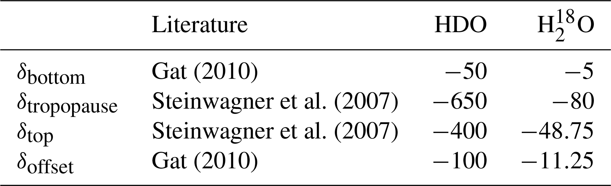
In the following sections, we present the first results and comparisons of model simulations with measurements spanning several spatiotemporal scales: Sect. 3.1 shows how the model-simulated diagnostic H2O can be used to investigate source regions of the (modeled) water cycle. Section 3.2 compares results for precipitation from the same long model integration with measurements taken from the GNIP network (IAEA/WMO, 2017; Terzer et al., 2013). Section 3.3 looks at seasonal and regional differences by comparing model output with pairs of {H2O,δD} derived from IASI satellite measurements (Schneider et al., 2016). Finally, Sect. 3.4 presents a first case study, in which simulated values of δD are compared with measurements from the IAGOS-CARIBIC project (Brenninkmeijer et al., 2007). All simulations discussed here are free-running.
In the following sections, we focus on H2O (ICON standard water), HDO and . The settings for each isotopologue are defined at runtime, which is why the specifications for the simulations are given here. The diffusion constant ratio is set to the values of Merlivat and Jouzel (1979) and the equilibrium fractionation is parameterized following Majoube (1971) over liquid water and following Merlivat and Nief (1967) over ice. Surface evaporation is described by the parameterization of Pfahl and Wernli (2009). The parameterization by Merlivat and Jouzel (1979) has little influence on the values in the free troposphere and is not discussed further. The dataset by LeGrande and Schmidt (2006) for the isotopic content of the ocean surface is used for all isotopologues. The grid-scale evaporation of hydrometeors is described by the parameterization by Stewart (1975) if not noted differently.
In addition to ICON standard water, three diagnostic sets of water tracers
are simulated. All fractionation is turned off, so they resemble H2O.
But the evaporation and initialization are different: water indexed by
init (as in qinit) is set to ICON water at initialization,
but evaporation is turned off. In the course of the simulation, water of
this type precipitates out of the model atmosphere. Water indexed by
ocn and lnd is initialized with zero and evaporates from
the ocean (qocn) and land areas (qlnd), respectively. The
sum of qinit, qocn and qlnd always equals the
mass mixing ratio of ICON standard water, indexed as qICON. These
tracers allow us to infer the relative importance of ocean and land
evaporation – essentially the source of water in the model atmosphere – at
all times. In addition to case studies, this is interesting because of the
simplified implementation of isotopic processes during land evaporation in
the current version of ICON-ART-Iso; see Sect. 2.3. The
tracers of qinit provide information on the importance of the
initialization at a certain time in the simulation.
3.1 An application of diagnostic water tracers: precipitation source regions
This section examines the moisture source regions of precipitation over ocean and land. Gimeno et al. (2012) give a review of the subject, while, e.g., Numaguti (1999), Van der Ent et al. (2010) and Risi et al. (2013) study this question by use of other models and in more detail.
Here, we use a decadal model integration. The simulation was initialized with ECMWF (European Centre for Medium-Range Weather Forecasts) Integrated Forecast System (IFS) operational analysis data on 1 January 2007, 00:00 UTC, to simulate 11 years on an R2B04 grid (≈160 km horizontal resolution). The time step was set to 240 s (convection called every second step) and output was saved on a regular grid every 10 h in order to obtain values from all times of the day. Sea surface temperatures and sea ice cover were updated daily by linearly interpolating monthly data provided by the AMIP II project (Taylor et al., 2000). The first year is not considered as spin-up time of the model and the simulation is evaluated up to the end of 2017.
We look at the total precipitation P in Northern Hemisphere winter (December, January, February, denoted by DJF) and summer (June, July, August, denoted by JJA). Figure 1 displays zonal sums of Pinit, Pocn and Plnd relative to standard water precipitation PICON as a function of latitude. The sum of precipitation that originates from convection is also given for each water species. The top panels give winter values, while the bottom panels display the results for summer months.
The area covered by ocean is not equally distributed over different latitudinal bands, which is the reason why ocean and land points are considered separately. Panels (b) and (e) show the fraction of precipitation that has fallen over the ocean relative to the total precipitation and the area fraction of the ocean in each latitudinal band. Despite the characteristics of the different seasons, which will be discussed in the following paragraphs, the latitudinal distribution of the ocean area fraction largely determines the overall fraction of rain that falls over the ocean or over land. This is why the other panels display values of P relative to the sum over each compartment, not to the total sum.
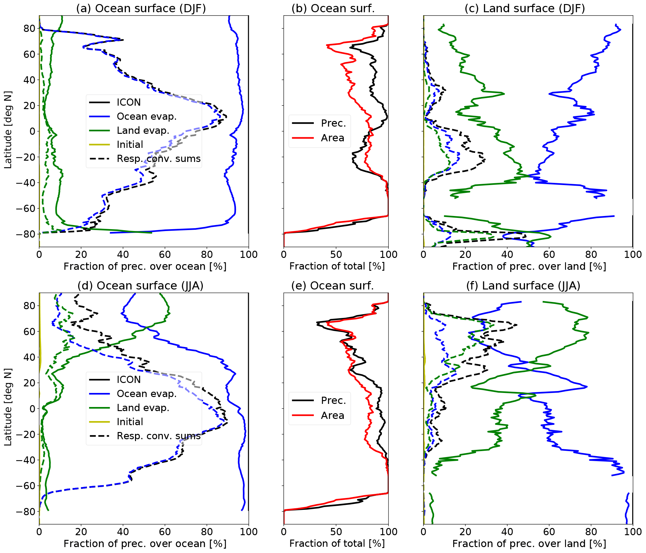
Figure 1Fractional contributions of PICON, Pinit, Pocn and Plnd to zonal sums of total precipitation for Northern Hemisphere winter (DJF, a–c) and summer (JJA, d–f) as a function of latitude. Outer panels show sums over the ocean and land grid points, respectively. Here, dashed lines indicate the contribution of convective precipitation for each source of atmospheric water. Center panels display the fraction of precipitation over the ocean relative to total precipitation (over land plus ocean) and the fraction of the area covered by ocean.
To evaluate the model simulation, we use values starting in the second year. At this time, the tropospheric moisture has been completely replaced by water that has evaporated during the model run. This is demonstrated by the values of Pinit close to zero in all panels in Fig. 1. Technically, this means that the ternary solution of qinit, qocn and qlnd that makes up qICON is practically reduced to a binary solution of only qocn and qlnd. Other experiments show that this is already true after a few weeks (not shown).
During Northern Hemisphere winter over the ocean (Fig. 1a), the precipitation is strongly dominated by water that has evaporated from the ocean. Water from the land surface hardly reaches the ocean. Over land areas, the ocean is also the dominant source for precipitation, reaching more than 50 % at almost all latitudes. In the Northern Hemisphere midlatitude land areas, more than 70 % of the precipitated water originates from the ocean. The tropical and Southern Hemisphere land areas (in DJF) receive up to 40 % of precipitation from land evaporation. Most precipitation at tropical and subtropical latitudes over the ocean originates from convection (indicated by dashed lines). The role of convection is much smaller over land areas and again stronger in the Southern Hemisphere. Note that in a simulation with very high horizontal resolution (Klocke et al., 2017), more convective processes could have been directly resolved. In this specific case of a resolution close to 160 km, practically no convection is directly resolved by the model. It should therefore be considered that the amount of precipitation from convection only shows the importance of this parameterization in the simulations at this resolution.
The distribution of precipitation water sources is different in Northern Hemisphere summer (bottom row of Fig. 1). In summer, the Northern Hemisphere land areas (bottom right) supply themselves with a substantial fraction of the moisture that then precipitates. The importance of convection is increased in Northern Hemisphere summer with its maximum influence shifted into northern midlatitudes. Despite the larger moisture availability over the ocean, the far Northern Hemisphere land areas also supply the larger part of moisture that precipitates over the ocean in summer; see Fig. 1d.
These results are comparable to the studies by Numaguti (1999), Van der Ent et al. (2010) and Risi et al. (2013). While these studies look at regional differences, the latitudinal dependence is similar to the results presented here. This first application of ICON-ART-Iso – while no isotopologues are used – shows how diagnostic moisture tracers can be applied to better understand specific aspects of the atmospheric water cycle.
3.2 The multi-annual simulation compared to GNIP data
For a first validation of δD and δ18O values, we use the decadal ICON-ART-Iso model integration of the previous section and compare results to data taken from the GNIP network (IAEA/WMO, 2017; Terzer et al., 2013). In this section, we analyze δ values in total precipitation.
Five GNIP stations were chosen for their good data availability in the respective years, sampling different climate zones: Vienna in eastern Austria (48.2∘ N, 16.3∘ E) in central Europe, Ankara in central Anatolia (40.0∘ N, 32.9∘ E), Bangkok in tropical southern Asia (13.7∘ N, 100.5∘ E), Puerto Montt in central Chile (41.5∘ S, 72.9∘ W) and Halley station in Antarctica (75.6∘ S, 20.6∘ W). The closest grid point to each of these stations was taken from the model output and the multiyear mean of each calendar month was calculated for δD, δ18O and d-excess (d-excess ) in precipitation, total precipitation P and 2 m temperature T2m. The corresponding values are available from GNIP. Results are displayed in Fig. 2. The panels for total precipitation also include the fractional contribution to precipitation by ocean and land evaporation (see previous section). All panels (except for the precipitation amount) show the 1σ standard deviation range for model and measurement data.

Figure 2Monthly mean data for five GNIP stations (left to right: Vienna, Ankara, Bangkok, Puerto Montt and Halley station). Variables listed from top to bottom: δD, δ18O, d-excess (δD−8 δ18O), total precipitation Ptot and 2 m temperature (T2m). Plots showing Ptot also include the percentage of land and ocean evaporation in precipitation. The 1σ standard deviation interval is indicated by dashed lines (except P for readability).
For most stations, the seasonal cycle of precipitation is reproduced by the model. This includes the summer minimum for Ankara and the strong winter precipitation in Puerto Montt. Precipitation is underestimated for Bangkok, especially in Northern Hemisphere spring. For all stations, the influence of land evaporation is strongest in their respective summer. Vienna and Ankara show a decreasing influence of the ocean in winter, typical for a more continental climate. For Puerto Montt, located between the Pacific and the Andean mountain range, and for Bangkok, almost all precipitating water originates from the ocean.
The seasonal cycle of temperature is reproduced for all stations. Winter temperatures are too cold in this model configuration for all stations. This temperature bias can partly be explained by the fact that the altitude of all stations is higher in the model because of the coarse grid, e.g., 550 m for the grid point identified with Vienna versus 198 m for the GNIP station. Also, the measured temperatures are slightly higher than mean monthly ERA-Interim (Dee et al., 2011) 2 m temperatures for the corresponding grid points (not shown).
Despite some biases, the mean values of δD and δ18O are well reproduced by ICON-ART-Iso for all five stations. The seasonal cycle is captured correctly in the Northern as well as the Southern Hemisphere. Values of d-excess are also of similar magnitude. Model data are more variable than the measurements. However, the model data are mostly within the standard deviation range of measurements. This demonstrates the capability of ICON-ART-Iso to simulate climatological patterns. The seasonal cycle and regional differences in δD and δ18O are correctly reproduced in this climatological integration.
3.3 Comparison with IASI satellite data for a seasonal perspective
Here, we compare pairs of {H2O,δD} retrieved from MetOp/IASI remote sensing measurements with data from two simulations. The section closely follows the case studies presented by Schneider et al. (2017), who compared IASI retrievals and data from the global hydrostatic model ECHAM5-wiso (Werner et al., 2011).
3.3.1 IASI satellite data and model post-processing
IASI (Infrared Atmospheric Sounding Interferometer) A and B are instruments onboard the MetOp-A and MetOp-B satellites (Schneider et al., 2016). They measure thermal infrared spectra in nadir view from which free-tropospheric {H2O,δD} pair data are derived. As the satellites circle the earth in polar sun-synchronous orbit, each IASI instrument takes measurements twice a day at local morning (approximately 09:30) and evening (approximately 21:30). The measurements are most sensitive at a height of approximately 4.9 km. An IASI {H2O,δD} pair retrieval method has been developed and validated in the framework of the project MUSICA (MUlti-platform remote Sensing of Isotopologues for investigating the Cycle of Atmospheric water). The MUSICA retrieval method is presented by Schneider and Hase (2011) and Wiegele et al. (2014) with updates given in Schneider et al. (2016).
Schneider et al. (2017) present guidelines for comparing model data to the remote sensing data. First, retrieval simulator software is used for simulating the MUSICA averaging kernel using the atmospheric state of the model atmosphere. The simulated kernel is then applied to the original model state (x) in order to calculate the state that would be reported by the satellite retrieval product (, see Eq. 23).
Here, A is the simulated averaging kernel and xa the a priori state. The a priori value used in the retrieval process for 4.9 km is at . This value represents the climatological state of the atmosphere. In the retrieval process, the satellite radiance measurements are used for estimating the deviation of the actual atmospheric state from the a priori assumed state, and it is important to note that the remote sensing retrieval product is not independent from the a priori assumptions (see Schneider et al., 2016, for more details). In Schneider et al. (2017), these guidelines have been followed for comparison of IASI data with ECHAM5-wiso model data. We use the same approach for comparisons to ICON-ART-Iso and our results can be directly compared to the results from the hydrostatic global model ECHAM5-wiso.
In order to compare ICON-ART-Iso measurements with IASI data, a simulation of 12 months is used, which was initialized on 5 November 2013. This simulation uses a finer resolution of R2B06, corresponding to roughly 40 km. Again, we use varying ocean surface temperatures and sea ice cover; see the specifications in Sect. 3.1. As in Schneider et al. (2017), two target time periods are investigated from 12–18 February and 12–18 August. As has been pointed out in Sect. 3.1, the amount of water remaining in the troposphere from initialization is negligible by using lead times of 3 months. For this study, model output was interpolated to a regular grid, which is close to the 40 km resolution of the numerical ICON grid in the tropics. Output was written for every hour of simulation.
IASI observations are only available at cloud-free conditions. In order to exclude cloud-affected grid points in the ICON data, the total cloud cover simulated by ICON was used, denoted by Cclct. All points with Cclct>90 % were excluded. The parameter Cclct goes into saturation quickly and 90 % is reached even for thin clouds. Surface emissivity Esrf is a necessary input parameter for the retrieval simulator. In this first study, Esrf was set to 0.96 over land and 0.975 over the ocean. This is in accordance with the mean values as given by Seemann et al. (2008). In addition, Schneider et al. (2017) show in a sensitivity study that errors on the order of 10 % in this value have only a limited influence on the averaging kernels as simulated by the retrieval simulator. We follow the method outlined by Schneider et al. (2017) and use values only when the sensitivity metric serr<0.05.
We examine results for different areas over ocean and over land using all data from the satellite and the model in the respective areas. The scatter of {H2O,δD} is not shown directly. Instead, the figures show the isolines of relative normalized frequency, which is explained in Appendix A. In addition, Rayleigh fractionation curves are indicated in all figures. These are the same as those given by Schneider et al. (2017).
3.3.2 Seasonal and daily cycle
Seasonal and daily cycle are investigated in {H2O,δD} space. The seasonal cycle is discussed for different regions over the central Pacific Ocean. The daily cycle is considered in the tropics and subtropics, also investigating differences between land and ocean areas.
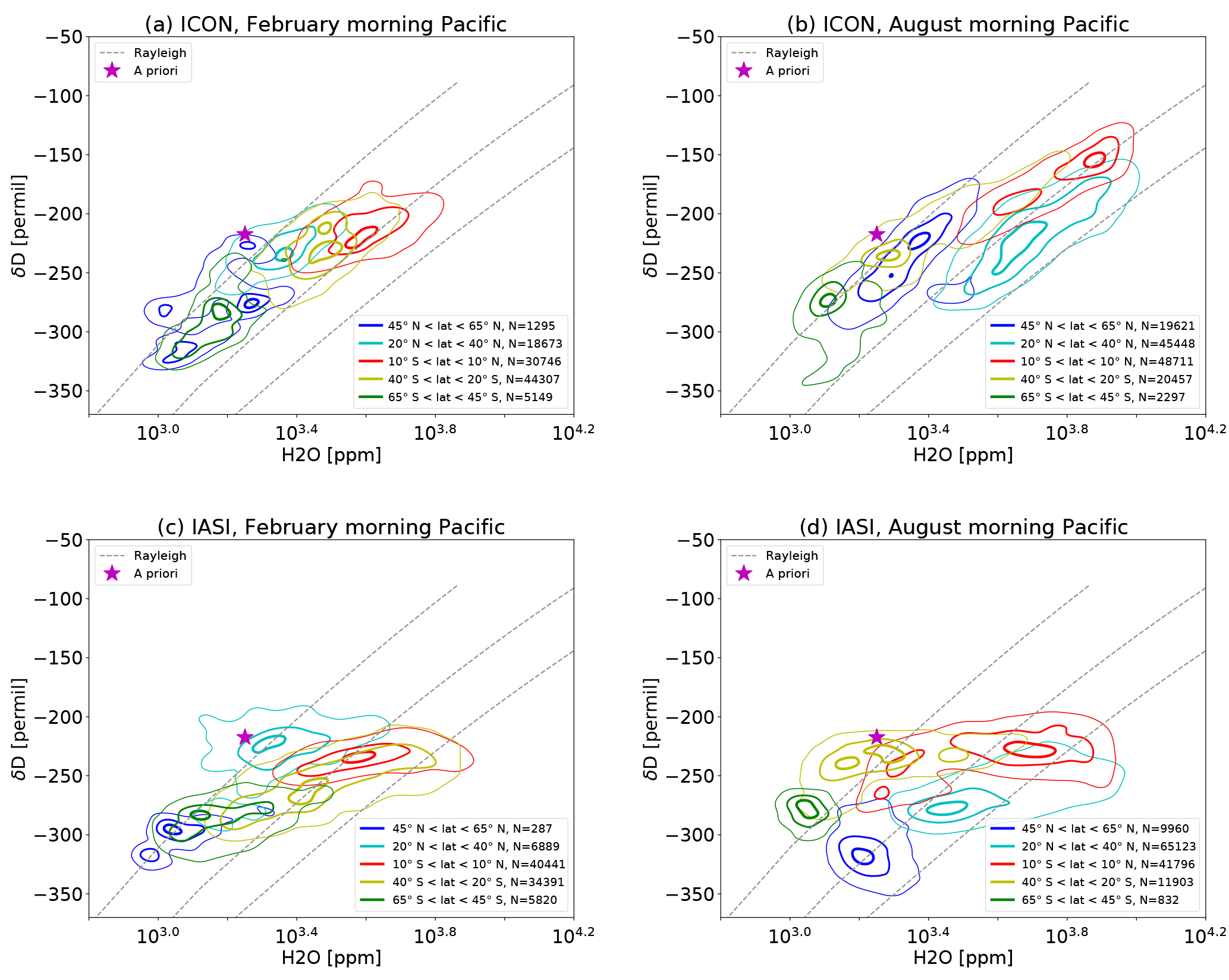
Figure 3Isolines of the relative normalized frequency distribution for pairs of δD and H2O (see Appendix A for the method) after processing ICON-ART-Iso data with the IASI retrieval simulator of Schneider et al. (2017) (a, b) and IASI data for the same time (c, d). Data from morning overpasses are shown for 12 to 18 February (a, c) and 12 to 18 August (b, d) 2014 for different latitudinal bands over the Pacific Ocean (140∘ E E longitude). Contour lines are indicated at 0.2, 0.6 and 0.9 of the normalized distribution.
First, the seasonal cycle over the Pacific Ocean is examined by comparing the two target periods in different areas (140∘ E E longitude and different latitudinal bins). Results are presented in Fig. 3, which includes the exact latitudes. IASI data (bottom panels) show the specific characteristics of the different regions. H2O content is highest for tropical air masses and lowest for the highest latitudes in February and August. At the same time, tropical air is least depleted in HDO, while the highest latitudes show the lowest values of δD, i.e., are more depleted. When comparing February and August values at each latitude, a clear seasonal signal appears everywhere except for the tropics: during summer of the corresponding hemisphere, the air is more humid and more depleted in HDO. The distributions seem to shift from season to season along a line perpendicular to those of the Rayleigh model. The distribution in the tropics shows a broadened shape in August.
The results of ICON-ART-Iso are shown in the top panels of Fig. 3. The latitudinal dependence is similar to IASI: high H2O and δD in the tropics and lower values for midlatitudes. The range of values is also very similar. The seasonal cycle in H2O and δD is also reproduced to some degree, especially in the subtropical latitudes. The most obvious differences to IASI results occur in the Northern Hemisphere midlatitudes in summer, which show less negative values of δD in the model than in the satellite data, especially for humid situations. In winter, this may also be the case, but there are only a few humid values simulated at all or available in the satellite dataset. In general, the model shows a similar behavior as ECHAM5-wiso, the results of which are presented by Schneider et al. (2017).
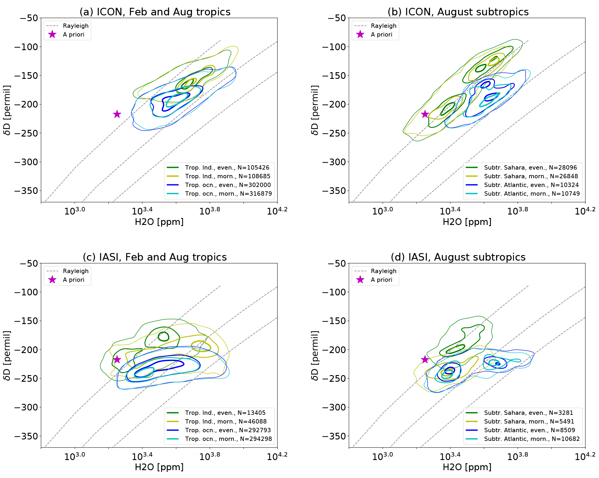
Figure 4Isolines of the relative normalized frequency distribution for pairs of δD and H2O (see Appendix A for the method) after processing ICON-ART-Iso data with the IASI retrieval simulator of Schneider et al. (2017) (a, b) and IASI data for the same time (c, d). (a, c) Data corresponding to morning and evening overpasses for the tropics (10∘ S N, all longitudes, summer and winter simulation) over land and over the ocean. (b, d) Morning and evening overpasses for the subtropics (22.5∘ S N, summer simulation) over land (Saharan desert region, 10∘ W E) and Atlantic Ocean (50∘ W W). Contour lines are indicated at 0.2, 0.6 and 0.9 of the normalized distribution.
For the daily cycle in the tropics and subtropics, land and ocean points are considered separately (Fig. 4; see caption for exact definition of the bins). IASI shows a clear signal of the daily cycle for both the tropics and subtropics over land (bottom panels of Fig. 4). There is no such signal over the ocean, where morning and evening distributions are almost identical. Over land, the water vapor in the tropics and subtropics is more depleted of HDO in the morning. There is also a daily cycle in H2O in the tropics: during morning overpasses, H2O values are higher than in the evening. Schneider et al. (2017) argue that this is due to the cloud filter, which removes areas of heavy convection in the evening. In the morning, the clouds have disappeared, but high humidity remains, especially in the lower troposphere. This may partly be due to evaporation of raindrops, which explains the enhanced depletion in HDO (Worden et al., 2007). Over the Sahara (the subtropical land area considered), the daily cycle is different: while mixing ratios of H2O rise only slightly during the day, there is a strong increase in the HDO content in the evening. This behavior can be attributed to vertical mixing (Schneider et al., 2017).
The data retrieved from ICON-ART-Iso model simulations are shown in the top panels of Fig. 4. Tropical air (panel a) over the land shows slightly lower mixing ratios for H2O than IASI. The humidity of tropical ocean points is better reproduced. The difference in δD is stronger for both areas, with δD values being too high in the model. There is no daily cycle in the tropics for ICON-ART-Iso. The subtropical mixing ratios (panel b) of H2O over the ocean are similar to those in the tropics but cover a smaller range than those retrieved from IASI. The very humid and very dry parts of the IASI distribution are not reproduced by the model. δD values in ICON-ART-Iso are larger than in the IASI retrievals. As pointed out by Schneider et al. (2017), the daily cycle in IASI also manifests itself in the number of samples passing the IASI cloud filter and quality control. The IASI cloud filter removes much more evening observations than morning observations, meaning more cloud coverage in the evening than in the morning. In contrast, the ICON-ART-Iso cloud filter removes a similar amount of data for morning and evening; i.e., in the model morning and evening cloud coverage is rather similar. This may also influence the results.
To further analyze the influence of ocean and land areas, the analysis of the daily cycle is repeated, making use of the humidity tracers qocn and qlnd. As has been pointed out in Sect. 3.1, qinit is negligible 3 months after initialization. To distinguish between grid points mostly influenced by ocean or land evaporation, we additionally use the following criteria to define ocean and land points: for grid points over the ocean and for land grid points predominantly affected by land evaporation. This investigation serves to showcase how the ocean and land evaporation tracers can be used and the threshold values are therefore arbitrary to some degree. The tracer fields of water evaporating from ocean and land have not been processed with the retrieval simulator, and instead values interpolated to 4.9 km are directly used.

Figure 5As Fig. 4 for ICON-ART-Iso. In addition to the land–ocean mask, land data must pass the condition and ocean data must pass .
The result is shown in Fig. 5 for the tropics and subtropics using the same method as for Fig. 4. The characteristics of the different regions show up much more clearly with the additional criteria. For the tropical ocean, the distribution of H2O is similar, but the values are slightly more depleted in HDO. The distribution of pairs attributed to the land surface is reduced to values with relatively high humidity and enriched in HDO. The latter might be due to the signal of plant evapotranspiration, which is considered a non-fractionation process.
In the subtropics, the distributions over land change their shape completely and are separated from those over the ocean. The distribution for the subtropical ocean remains largely unchanged, becoming slightly more elongated with lower values in δD. For the land surface, the additional criterion strongly reduces the number of values that are considered. This implies that over the Saharan desert, air mostly influenced by land evaporation (50 % or more) is very dry and highly processed (low δD).
This section shows that ICON-ART-Iso is able to reproduce regional differences and the seasonal cycle of {H2O,δD} of vapor in the lower troposphere. The additional water diagnostics are used to study the behavior of the model in more detail and will help investigate measured distributions in future studies.
3.4 Comparing with in situ IAGOS-CARIBIC measurements
In this section, we present a first case study, in which results of ICON-ART-Iso are compared to in situ measurements of δD taken by the IAGOS-CARIBIC passenger aircraft at 9–12 km of altitude. Two flights in September 2010 are considered, which took place a few days after the passage of the tropical cyclone Igor over the Atlantic Ocean. The full dataset of all δD measurements taken by IAGOS-CARIBIC in the tropics is also used as a reference.
3.4.1 IAGOS-CARIBIC data and model post-processing
In the European research infrastructure IAGOS-CARIBIC, a laboratory equipped with 15 instruments is deployed onboard a Lufthansa A340-600 for four intercontinental flights per month. Measurements of up to 100 trace gases and aerosol parameters are taken in situ and in air samples (Brenninkmeijer et al., 2007). δD is measured using the instrument ISOWAT (Dyroff et al., 2010). It is a tunable diode-laser absorption spectrometer that simultaneously measures HDO and H2O at wave numbers near 3765 cm−1 to derive δD in vapor. The instrument is calibrated based on regular measurements (each 30 min) of a water vapor standard with 500 ppm H2O and ‰. The δD offset is derived by considering the data of the driest 5 % of the air masses sampled during each flight, which is typically 4–8 ppm H2O. At the flight altitude of 10–12 km, this is without exception lowermost stratospheric air (LMS), for which a δD of −600 ‰ is assumed (Pollock et al., 1980; Randel et al., 2012). An assumed uncertainty of this LMS value of 400 ‰ translates to a relevant uncertainty of 20 ‰ at 100 ppm H2O. Due to further sources of measurement uncertainty, the data have a total flight-specific systematic uncertainty up to 100 ‰. The total uncertainty is humidity dependent, decreasing towards higher humidity (e.g., 100 ‰ at 80 ppm H2O versus less than 20 ‰ at 500 ppm H2O; see Christner, 2015, for more details).
The in situ IAGOS-CARIBIC data are suitable for the analysis of processes on small scales. δD measurements are available as 1 min means, which translates to a spatial scale of approximately 15 km. This horizontal resolution is finer than the chosen ICON-ART-Iso configuration (R2B06 corresponding to 40 km) and is therefore suitable for a case study validation. Unfortunately, the uncertainty of δD data at humidity below approximately 40 ppm H2O is too high to be used for analysis. Because of the systematic total uncertainty (see above), we use mean δD values from two flights through similar conditions.
In this section, measurements from a return flight from Frankfurt to Caracas on 22 September 2010 are analyzed (IAGOS-CARIBIC flight nos. 309 and 310, taking off at 10:16 UTC in Frankfurt and 22:12 UTC in Caracas, respectively). The two flights crossed the Atlantic approximately 2 days after Hurricane Igor had passed the flight track. The storm caused large-scale lofting of tropospheric air masses and a moistening at flight level. The high humidity at flight level (9–12 km) allowed many accurate δD measurements to be taken.
An ICON-ART-Iso simulation was initialized with ECMWF IFS analysis data from 12 September 2010 and with the isotope values initialized as explained in Sect. 2.7. This corresponds to a 10-day forecast for the time of the two flights. In this case, not all tropospheric water from the initialization has been replaced by water evaporated during the simulation at the time of analysis. However, the δD values adjust to local meteorology within a few days, developing realistic horizontal and vertical gradients. The simulation was set up on an R2B06 grid (≈40 km) with a time step of 240 s (convection called every second step). The output with a frequency of one snapshot per 15 min was examined on a 0.5∘ regular grid and interpolated linearly to the position of the aircraft. Figure 6 shows δD in water vapor in the upper troposphere roughly 24 h before the flights cross the Atlantic. The vortex signal of the hurricane clearly shows up in the δD field. The flight paths are also indicated in Fig. 6.
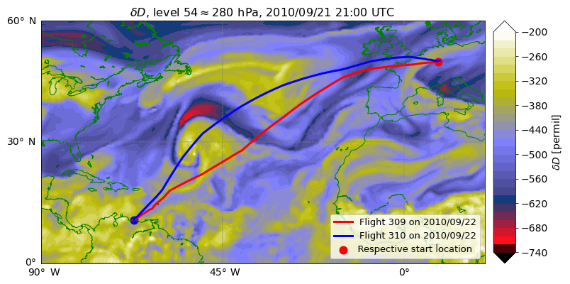
Figure 6δD in water vapor on model level 54 (≈260 hPa) on 21 September, 21:00 UTC, the date prior to that of the IAGOS-CARIBIC flights. The storm is visible in the western half of the plotted area (center approximately at 30∘ N, 50∘ W). The flight paths of IAGOS-CARIBIC flights 309 and 310 are also indicated by two lines, for which the departure locations are emphasized.
3.4.2 Results for flights in tropical regions
In order to compare values influenced by Hurricane Igor, model and measurement data from flights 309 and 310 are considered in latitudes around the storm track only (0∘ N N). For reference, all tropical δD values from the IAGOS-CARIBIC database are also examined. To create a comparable dataset from model data, the results of the decadal simulation presented in Sect. 3.1 were interpolated to the location of these measurements and are treated in the same manner. As in Sect. 3.3, the distribution of pairs of {H2O,δD} are examined. The results are shown in Fig. 7.
The distribution of IAGOS-CARIBIC δD measurements is shown in the left panel of Fig. 7. The tropical measurement sample (blue contours) consists of all relevant measurements (23.5∘ S N). While most tropical values are centered around −500 ‰ in δD and 100 to 150 ppm H2O, there is also a tail towards more humid pairs in the distribution. The lower limit in δD follows the curves of Rayleigh fractionation. The measurement data from flights 309 and 310 (red contours) show different characteristics. The range in H2O is similar to the maximum density of all tropical values, but the samples are more depleted in HDO. The humid branch is not continuous and the area of high humidity is sparsely populated. In general, both distributions are limited by the detection limit of 40 ppm in H2O, while contour lines may reach slightly lower values because of the smoothing that is applied in processing the data (see Appendix A).
Model results are shown in the right panel of Fig. 7. For this figure, model data along the flight tracks are used only when accurate δD measurements are available. A limit of 40 ppm is also applied to the model data. The isolines stretching to lower value pairs again result from smoothing the data.

Figure 7Isolines of the relative normalized frequency distribution (contours at 0.05, 0.4 and 0.9; see Appendix A for the method) of IAGOS-CARIBIC measurements (left) and ICON-ART-Iso model simulations for tropical samples, interpolated onto the paths of two IAGOS-CARIBIC flights 309–310 (right). The total number of data points in each distribution is given by the value N. Model data are considered only in locations with measurements, and the H2O measurement limit of 40 ppm is also considered in model data.
The distribution from the tropical model sample is in some ways similar to the one by all tropical IAGOS-CARIBIC measurements (comparing the blue contours of the two panels): there is a tail towards high humidities and the upper limit of δD is roughly at −400 ‰, while the lower limit is given by the second Rayleigh curve. The model sample is 4 % lower in δD on average (H2O reduced by 18 %). The mean for all values within the lowest density contour in {H2O,δD} is at for measurements, while it is at for the model sample and for measurements versus in the case of the highest density contour.
The main characteristics of the distribution for the two flights following Hurricane Igor are captured by the model ICON-ART-Iso (comparing the red contours of the two panels) and the center of the distribution is below the full tropical sample. The model sample is slightly reduced in δD (1.1 %) when comparing to the full tropical sample, but 12.3 % more humid. From this simulation and these measurements alone, it is difficult to say if these discrepancies result from errors in the meteorological representation of the hurricane or in the physical parameterizations of the model. The good agreement between model and measurements in general is promising, while details will need to be examined in future studies.
By using the other three diagnostic moisture tracers (initialization water qinit and water evaporating from the ocean and land, qocn and qlnd), the model results are examined further. The two transatlantic flights spent little time over land areas. Accordingly, only reaches an average of 2.8 % for both flights, 19.9 % at maximum. An average of 47.2 % of the sampled water originates from the initialization (59.6 % maximum), while the remainder has evaporated from the ocean in the course of the simulation. Part of the discrepancies between model and measurements may thus result from the simplified representation of δD in the initial vapor field, while the influence of the approximated land surface isotope values remains limited.
This is analyzed in more detail in Fig. 8. Values of δD and H2O along the flight paths are combined with information on the origin of the water that is sampled in the model. W stands for the ratio of vapor that originates from land or ocean evaporation or initialization, e.g., . In Fig. 8, the scatter is color-coded by Wocn. Because Wlnd is very low during most parts of the flights and especially so over the ocean, is a good approximation. In Fig. 8, green indicates Wlnd>10 %, when the approximation of a binary solution is not valid.
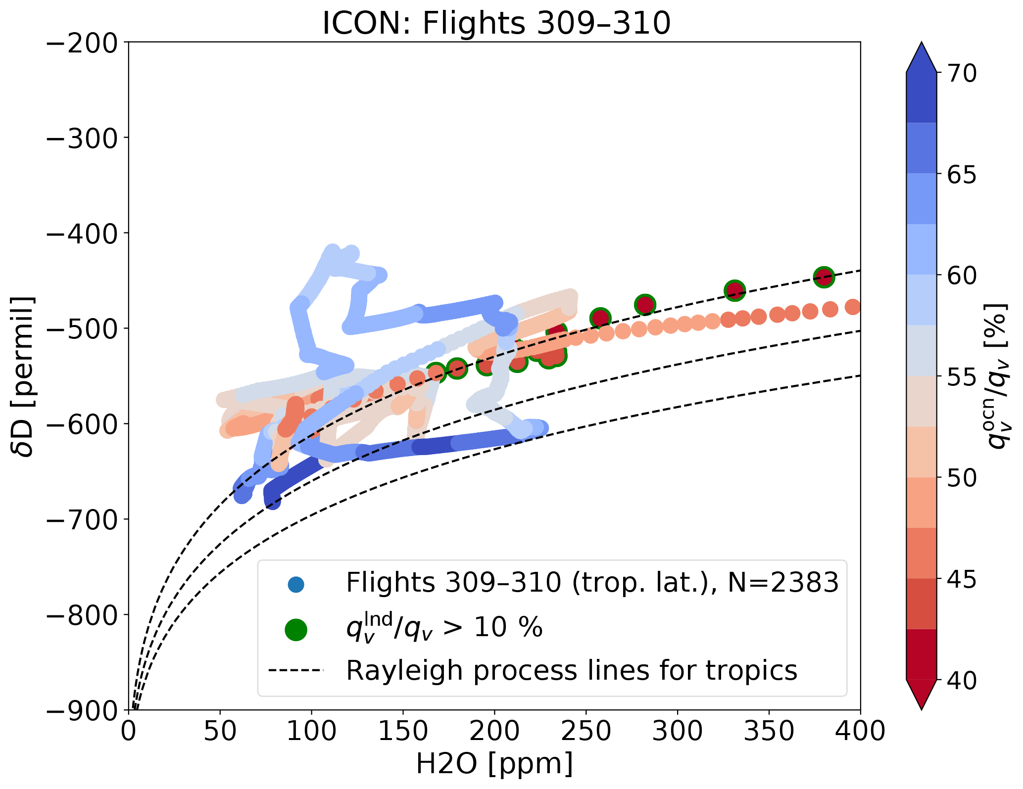
Figure 8Scatter of δD against H2O from ICON-ART-Iso interpolated to the flight paths of IAGOS-CARIBIC flights 309 and 310. Color coding indicates the ratio of in percent. Locations with Wlnd>10 % are marked in green. Values are considered for which p<280 hPa.
Figure 8 shows the strong influence of the ocean. More than 50 % of the sampled vapor originates from ocean evaporation for long parts of the flights. Values with the highest values of Winit (low Wocn) mostly follow the course of the Rayleigh fractionation lines. The lowest and highest values in δD are reached when Wocn is high (low values of Winit), indicating that the isotopologues in the model have seen many fractionating and transport processes. This includes air mass mixing, but also the microphysical and convective processes that are imprinted on the isotopologue ratio. The exact nature of these processes remains to be investigated in future studies.
We present ICON-ART-Iso, the isotope-enabled version of the global atmospheric model ICON (Zängl et al., 2015). We describe the model formulation as well as a set of evaluation studies. By using parts of the ICON-ART infrastructure (Schröter et al., 2018), the model is very flexible in terms of the simulated moisture tracers. These can be set to resemble either H2O (tagged water) or the stable isotopologues HDO or if fractionation is turned on. The physics of fractionation are largely based on the model COSMOiso (Pfahl et al., 2012). The first part of this article gives a detailed explanation of the parameterizations that have been implemented in ICON-ART-Iso to simulate the fractionation of water isotopologues.
We first evaluate tagged H2O tracers of moisture evaporating from land and ocean to investigate the moisture sources of precipitation. This demonstrates the capabilities of ICON-ART-Iso to use tagged water as an additional diagnostic. The latitudinal dependence is similar to that given by other studies (Risi et al., 2013). The following three sections then investigated the performance of the model for the simulation of the isotopologues considering (i) multi-annual, (ii) regional and (iii) mesoscale applications.
For a multi-annual evaluation, the simulated isotopologues HDO and from a decadal simulation on a relatively coarse grid (160 km horizontal resolution) are compared to measurements taken from the network of GNIP stations (IAEA/WMO, 2017; Terzer et al., 2013). The model simulates δD and δ18O reasonably well, reproducing the seasonal cycle of δ18O and the range in d-excess for different stations in the Northern and Southern Hemisphere. This investigation presents a first climatological application.
Regional differences in pairs of {H2O,δD} in lower free-tropospheric water vapor are then compared to data retrieved from IASI satellite measurements for a summer and winter case (Schneider and Hase, 2011; Schneider et al., 2016, 2017; Wiegele et al., 2014). The latitudinal dependence of these pairs is comparable to those from IASI retrievals. The seasonal cycle over the Pacific Ocean and the overall values are reproduced by the model in both seasons. The difference between land and ocean surfaces in the tropics and subtropics in the model is of similar magnitude as in the measurements. However, the daily cycle that is observed in the satellite data is not reproduced in the model. Overall, the performance is similar to that of ECHAM5-wiso (Schneider et al., 2017; Werner et al., 2011).
In a mesoscale application, a first comparison with in situ measurements uses δD in upper-tropospheric water vapor from two IAGOS-CARIBIC flights (Brenninkmeijer et al., 2007) transecting the Atlantic and from all tropical IAGOS-CARIBIC δD measurements (Dyroff et al., 2010). ICON-ART-Iso is able to reproduce the general features of the tropical IAGOS-CARIBIC dataset. The characteristics of the samples taken during two flights shortly after Hurricane Igor in September 2010 are also captured by the model.
In all three applications, the tagged evaporation water from ocean or land surfaces proves to be a valuable tool. It reveals a seasonal cycle in the precipitation water origin or shows the influence of initialization in the case of the comparison with IAGOS-CARIBIC data.
ICON-ART-Iso is a promising tool for future investigations of the atmospheric water cycle. This study demonstrates the flexibility of ICON-ART-Iso in terms of the setup for different diagnostics but also in terms of horizontal resolution and timescale. For future applications, it will be interesting to use a nudging of meteorological variables towards analysis data to facilitate comparisons with measurements in different case studies. Fractionation will be implemented in different microphysical schemes to make the model numerically more efficient and even better applicable for climatological questions. Due to its flexible setup, ICON-ART-Iso is ready to simulate tracers corresponding to or to be used as a test bed for new microphysical parameterizations.
The CARIBIC measurement data analyzed in this paper can be accessed by signing the CARIBIC data protocol, which can be downloaded at http://www.caribic-atmospheric.com/ (last access: 10 December 2018). The ICON code can be obtained from DWD after signing the license agreement available from icon@dwd.de. The ICON-ART code can be obtained after signing the license agreement available from bernhard.vogel@kit.edu.
Section 3.3 and 3.4 show and discuss distributions of {H2O,δD}. The scatter of {H2O,δD} is not shown directly as the figures would be too cluttered. Instead, the normalized relative frequency is discussed, the isolines of which are shown in the different figures. This method has been adopted from Christner (2015). Figure A1 shows the scatter and the isolines of normalized relative frequency for the IAGOS-CARIBIC measurements of flights 309–310, which are discussed in Sect. 3.4.
To arrive at the isolines, the data are binned in H2O and δD on a grid of 5 ppm ×5 ‰. In the case of IASI data, the data are binned in log10H2O (ppm) × δD on a grid of 0.05×5. Histogram counts are then interpolated onto a 1000×1000 grid. This is smoothed with a Gaussian filter with a standard deviation of 20 (15 in the case of IASI). These smoothed data are then normalized by the sum of all value pairs and normalized by the maximum value. Within this array of smoothed counts, isolines are drawn at 0.9, 0.4 and 0.05 (0.9, 0.6 and 0.2 in the case of IASI).
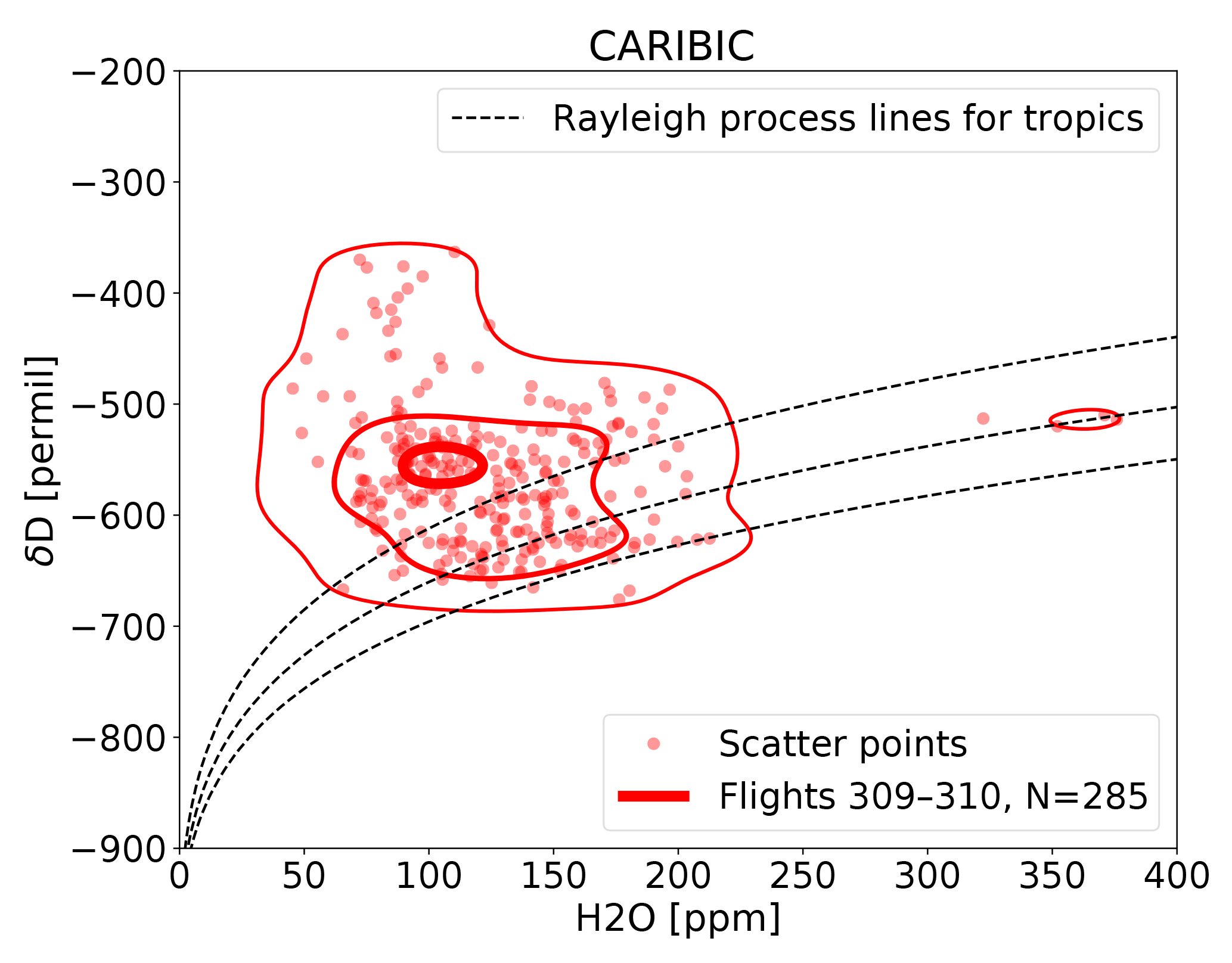
Figure A1Scatter and isolines of the relative normalized frequency distribution for tropical (latitude N) measurements of δD and H2O from IAGOS-CARIBIC flights 309 and 310 (September 2010). The figure demonstrates how the isolines (indicated at 0.1, 0.4 and 0.9) relate to the underlying scatter.
For evaporation and equilibration of rain and melting hydrometeors, the parameterization following Stewart (1975) has been presented in this paper; see Sect. 2.5 and Eq. (6) therein. As an alternative, we have also implemented the parameterization by Blossey et al. (2010). For completeness, this parameterization is given in Eq. (B1). In order to make a comparison easy, Eq. (B2) again states the parameterization by Stewart (1975). As above, both are given in the formulation for the evaporation of rain. The notation is the same as in the main body text.
By the above formulation, the difference of the two parameterizations is easily accessible. While the empirical equation by Stewart (1975) introduces the exponent n, which is determined by measurements, the parameterization by Blossey et al. (2010) modulates the saturation difference by a factor determined by the actual isotopologue ratios in the hydrometeor and the surrounding vapor. The ratio of ventilation factors f is an additional tuning parameter in the parameterization by Blossey et al. (2010), which is set to 1 in the standard setup. A detailed comparison to the results of Stewart (1975) is postponed to a later study in order to keep this paper concise.
JE programmed ICON-ART-Iso as an extension to ICON, performed and evaluated the simulations, and prepared the paper. This was done with RR as the main and PB as the overall advisor. SP provided the code of COSMOiso and helped in understanding and implementing the fractionating code. CD has taken over the work on ICON-ART-Iso and implemented some of the features after submission to GMDD. DR was the main contact person at DWD and helped with the model ICON. DR and JS aided in the technical development of the ICON-ART part of the model code and helped to solve many technical problems during the development of ICON-ART-Iso. EC provided and discussed data and the results of the comparison with IAGOS-CARIBIC. AZ is the coordinator of IAGOS-CARIBIC. CD was responsible for setting up and maintaining the instrument ISOWAT. MS provided data and discussed the results of the comparison with IASI satellite data.
The authors declare that they have no conflict of interest.
The authors would like to thank three anonymous reviewers for their helpful
comments on the paper and Axel Lauer for taking over the editorship. We would
also like to thank Axel Seifert and Matthias Raschendorfer of DWD for
discussions and help with parts of the ICON model code. This work was partly
performed on the computational resource ForHLR II funded by the Ministry of
Science, Research and the Arts Baden-Württemberg and DFG (Deutsche
Forschungsgemeinschaft). The MUSICA/IASI data have been produced in the
framework of the projects MUSICA (funded by the European Research Council
under the European Community's Seventh Framework Programme (FP7, 2007–2013),
ERC grant agreement number 256961) and MOTIV (funded by the Deutsche
Forschungsgemeinschaft under GZ SCHN 1126/2-1). We thank all the members of
the IAGOS-CARIBIC team. The collaboration with Lufthansa and Lufthansa
Technik and the financial support from the German Ministry for Education and
Science (grant 01LK1301C) are gratefully acknowledged.
The article processing charges for this
open-access
publication were covered by a Research
Centre of the Helmholtz
Association.
Edited by: Axel Lauer
Reviewed by: three anonymous referees
Bechtold, P., Semane, N., Lopez, P., Chaboureau, J.-P., Beljaars, A., and Bormann, N.: Representing equilibrium and nonequilibrium convection in large-scale models, J. Atmos. Sci., 71, 734–753, 2014. a
Blossey, P. N., Kuang, Z., and Romps, D. M.: Isotopic composition of water in the tropical tropopause layer in cloud-resolving simulations of an idealized tropical circulation, J. Geophys. Res.-Atmos., 115, D24309, https://doi.org/10.1029/2010JD014554, 2010. a, b, c, d, e, f, g, h, i, j
Bosilovich, M. G. and Schubert, S. D.: Water vapor tracers as diagnostics of the regional hydrologic cycle, J. Hydrometeorol., 3, 149–165, 2002. a
Brenninkmeijer, C. A. M., Crutzen, P., Boumard, F., Dauer, T., Dix, B., Ebinghaus, R., Filippi, D., Fischer, H., Franke, H., Frieß, U., Heintzenberg, J., Helleis, F., Hermann, M., Kock, H. H., Koeppel, C., Lelieveld, J., Leuenberger, M., Martinsson, B. G., Miemczyk, S., Moret, H. P., Nguyen, H. N., Nyfeler, P., Oram, D., O'Sullivan, D., Penkett, S., Platt, U., Pupek, M., Ramonet, M., Randa, B., Reichelt, M., Rhee, T. S., Rohwer, J., Rosenfeld, K., Scharffe, D., Schlager, H., Schumann, U., Slemr, F., Sprung, D., Stock, P., Thaler, R., Valentino, F., van Velthoven, P., Waibel, A., Wandel, A., Waschitschek, K., Wiedensohler, A., Xueref-Remy, I., Zahn, A., Zech, U., and Ziereis, H.: Civil Aircraft for the regular investigation of the atmosphere based on an instrumented container: The new CARIBIC system, Atmos. Chem. Phys., 7, 4953–4976, https://doi.org/10.5194/acp-7-4953-2007, 2007. a, b, c
Cappa, C. D., Hendricks, M. B., DePaolo, D. J., and Cohen, R. C.: Isotopic fractionation of water during evaporation, J. Geophys. Res.-Atmos., 108, 4525, https://doi.org/10.1029/2003JD003597, 2003. a
Christner, E.: Messungen von Wasserisotopologen von der planetaren Grenzschicht bis zur oberen Troposphäre zur Untersuchung des hydrologischen Kreislaufs, PhD thesis, KIT, IMK-ASF, H.-v.-Helmholtz-Platz 1, 76344 Leopoldshafen, 2015. a, b
Craig, H.: Isotopic variations in meteoric waters, Science, 133, 1702–1703, 1961. a, b, c
Craig, H. and Gordon, L.: Deuterium and oxygen 18 variations in the ocean and marine atmospher, in: Stable Isotopes in Oceanographic Studies and Paleotemperatures, edited by: Tongiogi, E., V. Lishi e F., Pisa, 9–130, 1965. a, b
Dansgaard, W.: The O18-abundance in fresh water, Geochim. Cosmochim. Ac., 6, 241–260, 1954. a, b
Dansgaard, W.: Stable isotopes in precipitation, Tellus, 16, 436–468, https://doi.org/10.3402/tellusa.v16i4.8993, 1964. a
Dee, D. P., Uppala, S. M., Simmons, A. J., Berrisford, P., Poli, P., Kobayashi, S., Andrae, U., Balmaseda, M. A., Balsamo, G., Bauer, P., Bechtold, P., Beljaars, A. C. M., van de Berg, L., Bidlot, J., Bormann, N., Delsol, C., Dragani, R., Fuentes, M., Geer, A. J., Haimberger, L., Healy, S. B., Hersbach, H., Hólm, E. V., Isaksen, L., Kållberg, P., Köhler, M., Matricardi, M., McNally, A. P., Monge-Sanz, B. M., Morcrette, J.-J., Park, B.-K., Peubey, C., de Rosnay, P., Tavolato, C., Thépaut, J.-N., and Vitart, F.: The ERA-Interim reanalysis: configuration and performance of the data assimilation system, Q. J. Roy. Meteor. Soc., 137, 553–597, https://doi.org/10.1002/qj.828, 2011. a
Dyroff, C., Fütterer, D., and Zahn, A.: Compact diode-laser spectrometer ISOWAT for highly sensitive airborne measurements of water-isotope ratios, Appl. Phys. B, 98, 537–548, https://doi.org/10.1007/s00340-009-3775-6, 2010. a, b, c
Galewsky, J., Steen-Larsen, H. C., Field, R. D., Worden, J., Risi, C., and Schneider, M.: Stable isotopes in atmospheric water vapor and applications to the hydrologic cycle, Rev. Geophys., 54, 809–865, https://doi.org/10.1002/2015RG000512, 2016. a, b, c, d
Gat, J. R.: Oxygen and hydrogen isotopes in the hydrologic cycle, Annual Review of Earth and Planetary Sciences, 24, 225–262, 1996. a, b
Gat, J. R.: Isotope hydrology: a study of the water cycle, Series on environmental science and management, 6, Imperial College Press, London, 2010. a, b, c, d
Gimeno, L., Stohl, A., Trigo, R. M., Dominguez, F., Yoshimura, K., Yu, L., Drumond, A., Durán-Quesada, A. M., and Nieto, R.: Oceanic and terrestrial sources of continental precipitation, Rev. Geophys., 50, RG4003, https://doi.org/10.1029/2012RG000389, 2012. a
Gonfiantini, R., Stichler, W., and Rozanski, K.: Reference and intercomparison materials for stable isotopes of light elements, Tech. Rep. IAEA-TECDOC-825, International Atomic Energy Agency, 1993. a
Gunson, M. R., Abbas, M., Abrams, M., Allen, M., Brown, L., Brown, T., Chang, A., Goldman, A., Irion, F., Lowes, L., Mahieu, E., Manney, G. L., Michelsen, H. A., Newchurch, M. J., Rinsland, C. P., Salawitch, R. J., Stiller, G. P., Toon, G. C., Yung, Y. L., and Zander, R.: The Atmospheric Trace Molecule Spectroscopy (ATMOS) experiment: Deployment on the ATLAS space shuttle missions, Geophys. Res. Lett., 23, 2333–2336, 1996. a
Heinze, R., Dipankar, A., Henken, C., Moseley, C., Sourdeval, O., Trömel, S., Xie, X., Adamidis, P., Ament, F., Baars, H., Barthlott, C., Behrendt, A., Blahak, U., Bley, S., Brdar, S., Brueck, M., Crewell, S., Deneke, H., Di Girolamo, P., Evaristo, R., Fischer, J., Frank, C., Friederichs, P., Göcke, T., Gorges, K., Hande, L., Hanke, M., Hansen, A., Hege, H.-C., Hoose, C., Jahns, T., Kalthoff, N., Klocke, D., Kneifel, S., Knippertz, P., Kuhn, A., van Laar, T., Macke, A., Maurer, V., Mayer, B., Meyer, C., Muppa, S., Neggers, R. A. J., Orlandi, E., Pantillon, F., Pospichal, B., Röber, N., Scheck, L., Seifert, A., Seifert, P., Senf, F., Siligam, P., Simmer, C., Steinke, S., Stevens, B., Wapler, K., Weniger, M., Wulfmeyer, V., Zängl, G., Zhang, D., and Quaas, J.: Large-eddy simulations over Germany using ICON: a comprehensive evaluation, Q. J. Roy. Meteor. Soc., 143, 69–100, https://doi.org/10.1002/qj.2947, 2017. a, b
Holton, J. R. and Hakim, G. J.: An introduction to dynamic meteorology, Elsevier Academic Press, Amsterdam, 5th Edn., 2013. a
Holton, J. R., Haynes, P. H., McIntyre, M. E., Douglass, A. R., Rood, R. B., and Pfister, L.: Stratosphere-troposphere exchange, Rev. Geophys., 33, 403–439, 1995. a
Horita, J. and Wesolowski, D. J.: Liquid-vapor fractionation of oxygen and hydrogen isotopes of water from the freezing to the critical temperature, Geochim. Cosmochim. Ac., 58, 3425–3437, https://doi.org/10.1016/0016-7037(94)90096-5, 1994. a
IAEA/WMO: Global Network of Isotopes in Precipitation, The GNIP Database, available at: http://www-naweb.iaea.org/napc/ih/IHS_resources_gnip.html (last access: 10 December 2018), 2017. a, b, c
Jacob, D. J.: Introduction to atmospheric chemistry, Princeton Univ. Press, Princeton, NJ, 1999. a
Joussaume, S. and Jouzel, J.: Paleoclimatic tracers: An investigation using an atmospheric general circulation model under ice age conditions: 2. Water isotopes, J. Geophys. Res.-Atmos., 98, 2807–2830, https://doi.org/10.1029/92JD01920, 1993. a
Joussaume, S., Sadourny, R., and Jouzel, J.: A general circulation model of water isotope cycles in the atmosphere, Nature, 311, 24–29, 1984. a
Jouzel, J. and Merlivat, L.: Deuterium and oxygen 18 in precipitation: Modeling of the isotopic effects during snow formation, J. Geophys. Res.-Atmos., 89, 11749–11757, https://doi.org/10.1029/JD089iD07p11749, 1984. a, b
Jouzel, J., Merlivat, L., and Roth, E.: Isotopic study of hail, J. Geophys. Res., 80, 5015–5030, https://doi.org/10.1029/JC080i036p05015, 1975. a
Klocke, D., Brueck, M., Hohenegger, C., and Stevens, B.: Rediscovery of the doldrums in storm-resolving simulations over the tropical Atlantic, Nat. Geosci., 10, 891–896, 2017. a, b
Kraus, H.: Die Atmosphäre der Erde: eine Einführung in die Meteorologie, Springer, Berlin, 3rd Edn., 2004. a
Lauritzen, P. H., Ullrich, P. A., Jablonowski, C., Bosler, P. A., Calhoun, D., Conley, A. J., Enomoto, T., Dong, L., Dubey, S., Guba, O., Hansen, A. B., Kaas, E., Kent, J., Lamarque, J.-F., Prather, M. J., Reinert, D., Shashkin, V. V., Skamarock, W. C., Sørensen, B., Taylor, M. A., and Tolstykh, M. A.: A standard test case suite for two-dimensional linear transport on the sphere: results from a collection of state-of-the-art schemes, Geosci. Model Dev., 7, 105–145, https://doi.org/10.5194/gmd-7-105-2014, 2014. a
Lee, J.-E. and Fung, I.: “Amount effect” of water isotopes and quantitative analysis of post-condensation processes, Hydrol. Process., 22, 1–8, 2008. a
Lee, X., Sargent, S., Smith, R., and Tanner, B.: In Situ Measurement of the Water Vapor 18O∕16O Isotope Ratio for Atmospheric and Ecological Applications, J. Atmos. Ocean. Tech., 22, 555–565, https://doi.org/10.1175/JTECH1719.1, 2005. a
LeGrande, A. N. and Schmidt, G. A.: Global gridded data set of the oxygen isotopic composition in seawater, Geophys. Res. Lett., 33, L12604, https://doi.org/10.1029/2006GL026011, 2006. a, b
Majoube, M.: Fractionnement en oxygén 18 et in deutérium entre l'eau et sa vapeur, J. Chim. Phgys. PCB, 68, 1423–1436, 1971. a, b
Merlivat, L. and Jouzel, J.: Global climatic interpretation of the deuterium-oxygen 18 relationship for precipitation, J. Geophys. Res.-Oceans, 84, 5029–5033, 1979. a, b, c, d, e
Merlivat, L. and Nief, G.: Fractionnement isotopique lors des changements d'état solide-vapeur et liquide-vapeur de l'eau à des températures inférieures à 0 C, Tellus, 19, 122–127, 1967. a, b
Mook, W. G.: Environmental isotopes in the hydrological cycle, Principles and Applications, vol. 2, International Atomic Energy Agency, UNESCO, Paris, 2001. a
Morrison, H., Jensen, A. A., Harrington, J. Y., and Milbrandt, J. A.: Advection of Coupled Hydrometeor Quantities in Bulk Cloud Microphysics Schemes, Mon. Weather Rev., 144, 2809–2829, https://doi.org/10.1175/MWR-D-15-0368.1, 2016. a
Numaguti, A.: Origin and recycling processes of precipitating water over the Eurasian continent: Experiments using an atmospheric general circulation model, J. Geophys. Res.-Atmos., 104, 1957–1972, 1999. a, b
Pfahl, S. and Wernli, H.: Lagrangian simulations of stable isotopes in water vapor: An evaluation of nonequilibrium fractionation in the Craig-Gordon model, J. Geophys. Res.-Atmos., 114, D20108, https://doi.org/10.1029/2009JD012054, 2009. a, b, c
Pfahl, S., Wernli, H., and Yoshimura, K.: The isotopic composition of precipitation from a winter storm – a case study with the limited-area model COSMOiso, Atmos. Chem. Phys., 12, 1629–1648, https://doi.org/10.5194/acp-12-1629-2012, 2012. a, b, c, d, e, f, g, h, i, j, k, l, m
Pinet, P. R.: Oceanography: an introduction to the planet oceanus, West Publishing, St. Paul, 2nd Edn., 1993. a
Pollock, W., Heidt, L. E., Lueb, R., and Ehhalt, D. H.: Measurement of stratospheric water vapor by cryogenic collection, J. Geophys. Res.-Oceans, 85, 5555–5568, https://doi.org/10.1029/JC085iC10p05555, 1980. a
Pruppacher, H. R. and Klett, J. D.: Microphysics of Clouds and Precipitation: Reprinted 1980, Springer Science & Business Media, 2012. a
Randel, W. J., Moyer, E., Park, M., Jensen, E., Bernath, P., Walker, K., and Boone, C.: Global variations of HDO and HDO∕H2O ratios in the upper troposphere and lower stratosphere derived from ACE-FTS satellite measurements, J. Geophys. Res.-Atmos., 117, D06303, https://doi.org/10.1029/2011JD016632, 2012. a
Rieger, D., Bangert, M., Bischoff-Gauss, I., Förstner, J., Lundgren, K., Reinert, D., Schröter, J., Vogel, H., Zängl, G., Ruhnke, R., and Vogel, B.: ICON–ART 1.0 – a new online–coupled model system from the global to regional scale, Geosci. Model Dev., 8, 1659–1676, https://doi.org/10.5194/gmd-8-1659-2015, 2015. a
Rieger, D., Steiner, A., Bachmann, V., Gasch, P., Förstner, J., Deetz, K., Vogel, B., and Vogel, H.: Impact of the 4 April 2014 Saharan dust outbreak on the photovoltaic power generation in Germany, Atmos. Chem. Phys., 17, 13391–13415, https://doi.org/10.5194/acp-17-13391-2017, 2017. a
Riese, M., Ploeger, F., Rap, A., Vogel, B., Konopka, P., Dameris, M., and Forster, P.: Impact of uncertainties in atmospheric mixing on simulated UTLS composition and related radiative effects, J. Geophys. Res.-Atmos., 117, D16305, https://doi.org/10.1029/2012JD017751, 2012. a
Risi, C., Bony, S., and Vimeux, F.: Influence of convective processes on the isotopic composition (δ18O and δD) of precipitation and water vapor in the tropics: 2. Physical interpretation of the amount effect, J. Geophys. Res.-Atmos., 113, D19306, https://doi.org/10.1029/2008JD009943, 2008. a
Risi, C., Bony, S., Vimeux, F., and Jouzel, J.: Water-stable isotopes in the LMDZ4 general circulation model: Model evaluation for present-day and past climates and applications to climatic interpretations of tropical isotopic records, J. Geophys. Res.-Atmos., 115, D12118, https://doi.org/10.1029/2009JD013255, 2010. a, b, c
Risi, C., Noone, D., Frankenberg, C., and Worden, J.: Role of continental recycling in intraseasonal variations of continental moisture as deduced from model simulations and water vapor isotopic measurements, Water Resour. Res., 49, 4136–4156, 2013. a, b, c
Schmidt, G. A., Ruedy, R. A., Miller, R. L., and Lacis, A. A.: Attribution of the present-day total greenhouse effect, J. Geophys. Res.-Atmos., 115, D20106, https://doi.org/10.1029/2010JD014287, 2010. a
Schneider, M. and Hase, F.: Optimal estimation of tropospheric H2O and δD with IASI/METOP, Atmos. Chem. Phys., 11, 11207–11220, https://doi.org/10.5194/acp-11-11207-2011, 2011. a, b, c
Schneider, M., Wiegele, A., Barthlott, S., González, Y., Christner, E., Dyroff, C., García, O. E., Hase, F., Blumenstock, T., Sepúlveda, E., Mengistu Tsidu, G., Takele Kenea, S., Rodríguez, S., and Andrey, J.: Accomplishments of the MUSICA project to provide accurate, long-term, global and high-resolution observations of tropospheric {H2O,δD} pairs – a review, Atmos. Meas. Tech., 9, 2845–2875, https://doi.org/10.5194/amt-9-2845-2016, 2016. a, b, c, d, e
Schneider, M., Borger, C., Wiegele, A., Hase, F., García, O. E., Sepúlveda, E., and Werner, M.: MUSICA MetOp/IASI {H2O,δD} pair retrieval simulations for validating tropospheric moisture pathways in atmospheric models, Atmos. Meas. Tech., 10, 507–525, https://doi.org/10.5194/amt-10-507-2017, 2017. a, b, c, d, e, f, g, h, i, j, k, l, m, n, o
Schröter, J., Rieger, D., Stassen, C., Vogel, H., Weimer, M., Werchner, S., Förstner, J., Prill, F., Reinert, D., Zängl, G., Giorgetta, M., Ruhnke, R., Vogel, B., and Braesicke, P.: ICON-ART 2.1: a flexible tracer framework and its application for composition studies in numerical weather forecasting and climate simulations, Geosci. Model Dev., 11, 4043–4068, https://doi.org/10.5194/gmd-11-4043-2018, 2018. a, b, c
Seemann, S. W., Borbas, E. E., Knuteson, R. O., Stephenson, G. R., and Huang, H.-L.: Development of a Global Infrared Land Surface Emissivity Database for Application to Clear Sky Sounding Retrievals from Multispectral Satellite Radiance Measurements, J. Appl. Meteorol. Clim., 47, 108–123, https://doi.org/10.1175/2007JAMC1590.1, 2008. a
Seifert, A.: On the Parameterization of Evaporation of Raindrops as Simulated by a One-Dimensional Rainshaft Model, J. Atmos. Sci., 65, 3608–3619, https://doi.org/10.1175/2008JAS2586.1, 2008. a
Seifert, A. and Beheng, K.: A two-moment cloud microphysics parameterization for mixed-phase clouds. Part 1: Model description, Meteorol. Atmos. Phys., 92, 45–66, 2006. a, b, c
Sherwood, S. C., Bony, S., and Dufresne, J.-L.: Spread in model climate sensitivity traced to atmospheric convective mixing, Nature, 505, 37–42, 2014. a
Shine, K. P. and Sinha, A.: Sensitivity of the Earth's climate to height-dependent changes in the water vapour mixing ratio, Nature, 354, 382–384, 1991. a
Souchez, R. and Jouzel, J.: On the isotopic composition in δD and δ18O of water and ice during freezing, J. Glaciol., 30, 369–372, 1984. a
Souchez, R., Jouzel, J., Lorrain, R., Sleewaegen, S., Stiévenard, M., and Verbeke, V.: A kinetic isotope effect during ice formation by water freezing, Geophys. Res. Lett., 27, 1923–1926, 2000. a
Steinwagner, J., Milz, M., von Clarmann, T., Glatthor, N., Grabowski, U., Höpfner, M., Stiller, G. P., and Röckmann, T.: HDO measurements with MIPAS, Atmos. Chem. Phys., 7, 2601–2615, https://doi.org/10.5194/acp-7-2601-2007, 2007. a, b, c, d
Stewart, M. K.: Stable isotope fractionation due to evaporation and isotopic exchange of falling waterdrops: Applications to atmospheric processes and evaporation of lakes, J. Geophys. Res., 80, 1133–1146, 1975. a, b, c, d, e, f, g, h, i, j, k
Taylor, K. E., Williamson, D., and Zwiers, F.: The sea surface temperature and sea-ice concentration boundary conditions for AMIP II simulations, Program for Climate Model Diagnosis and Intercomparison, Lawrence Livermore National Laboratory, University of California, 2000. a
Terzer, S., Wassenaar, L. I., Araguás-Araguás, L. J., and Aggarwal, P. K.: Global isoscapes for δ18O and δ2H in precipitation: improved prediction using regionalized climatic regression models, Hydrol. Earth Syst. Sci., 17, 4713–4728, https://doi.org/10.5194/hess-17-4713-2013, 2013. a, b, c
Tiedtke, M.: A comprehensive mass flux scheme for cumulus parameterization in large-scale models, Mon. Weather Rev., 117, 1779–1800, 1989. a, b
Van der Ent, R. J., Savenije, H. H., Schaefli, B., and Steele-Dunne, S. C.: Origin and fate of atmospheric moisture over continents, Water Resour. Res., 46, W09525, https://doi.org/10.1029/2010WR009127, 2010. a, b
Werner, M., Langebroek, P. M., Carlsen, T., Herold, M., and Lohmann, G.: Stable water isotopes in the ECHAM5 general circulation model: Toward high-resolution isotope modeling on a global scale, J. Geophys. Res.-Atmos, 116, D15109, https://doi.org/10.1029/2011JD015681, 2011. a, b, c, d
Wiegele, A., Schneider, M., Hase, F., Barthlott, S., García, O. E., Sepúlveda, E., González, Y., Blumenstock, T., Raffalski, U., Gisi, M., and Kohlhepp, R.: The MUSICA MetOp/IASI H2O and δD products: characterisation and long-term comparison to NDACC/FTIR data, Atmos. Meas. Tech., 7, 2719–2732, https://doi.org/10.5194/amt-7-2719-2014, 2014. a, b
Worden, J., Bowman, K., Noone, D., Beer, R., Clough, S., Eldering, A., Fisher, B., Goldman, A., Gunson, M., Herman, R., Kulawik, S. S., Lampel, M., Luo, M., Osterman, G., Rinsland, C., Rodgers, C., Sander, S., Shephard, M., and Worden, H.: Tropospheric Emission Spectrometer observations of the tropospheric HDO∕H2O ratio: Estimation approach and characterization, J. Geophys. Res.-Atmos., 111, D16309, https://doi.org/10.1029/2005JD006606, 2006. a
Worden, J., Noone, D., Bowman, K., Beer, R., Eldering, A., Fisher, B., Gunson, M., Goldman, A., Herman, R., Kulawik, S. S., et al.: Importance of rain evaporation and continental convection in the tropical water cycle, Nature, 445, 528–533, 2007. a
Zängl, G., Reinert, D., Rípodas, P., and Baldauf, M.: The ICON (ICOsahedral Non-hydrostatic) modelling framework of DWD and MPI-M: Description of the non-hydrostatic dynamical core, Q. J. Roy. Meteor. Soc., 141, 563–579, 2015. a, b, c, d, e
- Abstract
- Introduction
- The model ICON-ART-Iso
- Model evaluation results
- Conclusions
- Code and data availability
- Appendix A: Preparing the relative normalized frequency distributions
- Appendix B: Fractionation during evaporation of hydrometeors following Blossey et al. (2010)
- Author contributions
- Competing interests
- Acknowledgements
- References