the Creative Commons Attribution 4.0 License.
the Creative Commons Attribution 4.0 License.
 | 06 Dec 2018
Concentrations and radiative forcing of anthropogenic aerosols from 1750 to 2014 simulated with the Oslo CTM3 and CEDS emission inventory
Marianne Tronstad Lund
Gunnar Myhre
Amund Søvde Haslerud
Ragnhild Bieltvedt Skeie
Jan Griesfeller
Stephen Matthew Platt
Rajesh Kumar
Cathrine Lund Myhre
Michael Schulz
We document the ability of the new-generation Oslo chemistry-transport model, Oslo CTM3, to accurately simulate present-day aerosol distributions. The model is then used with the new Community Emission Data System (CEDS) historical emission inventory to provide updated time series of anthropogenic aerosol concentrations and consequent direct radiative forcing (RFari) from 1750 to 2014.
Overall, Oslo CTM3 performs well compared with measurements of surface concentrations and remotely sensed aerosol optical depth. Concentrations are underestimated in Asia, but the higher emissions in CEDS than previous inventories result in improvements compared to observations. The treatment of black carbon (BC) scavenging in Oslo CTM3 gives better agreement with observed vertical BC profiles relative to the predecessor Oslo CTM2. However, Arctic wintertime BC concentrations remain underestimated, and a range of sensitivity tests indicate that better physical understanding of processes associated with atmospheric BC processing is required to simultaneously reproduce both the observed features. Uncertainties in model input data, resolution, and scavenging affect the distribution of all aerosols species, especially at high latitudes and altitudes. However, we find no evidence of consistently better model performance across all observables and regions in the sensitivity tests than in the baseline configuration.
Using CEDS, we estimate a net RFari in 2014 relative to 1750 of −0.17 W m−2, significantly weaker than the IPCC AR5 2011–1750 estimate. Differences are attributable to several factors, including stronger absorption by organic aerosol, updated parameterization of BC absorption, and reduced sulfate cooling. The trend towards a weaker RFari over recent years is more pronounced than in the IPCC AR5, illustrating the importance of capturing recent regional emission changes.
- Article
(4479 KB) - Full-text XML
-
Supplement
(3876 KB) - BibTeX
- EndNote


Changes in anthropogenic emissions over the industrial period have significantly altered the abundance, composition, and properties of atmospheric aerosols, causing a change in the radiative energy balance. The net energy balance change is determined by a complex interplay of different types of aerosols and their interactions with radiation and clouds, causing both positive (warming) and negative (cooling) radiative impacts. Global aerosols were estimated by the Intergovernmental Panel on Climate Change Fifth Assessment Report (IPCC AR5) to have caused an effective radiative forcing (ERF) of −0.9 W m−2 over the industrial era from 1750 to 2011, but with considerable uncertainty (−1.9 to −0.1 W m−2) (Boucher et al., 2013). This large uncertainty range arises from a number of factors, including uncertainties in emissions and the simulated spatiotemporal distribution of aerosols and their chemical composition and properties.
Historical emission estimates for anthropogenic aerosol and precursor compounds are key data needed for climate and atmospheric chemistry-transport models in order to examine how these drivers have contributed to climate change. The Community Emissions Data System (CEDS) recently published a new time series of emissions from 1750 to 2014, which will be used in the upcoming CMIP6 (Hoesly et al., 2018). CEDS includes several improvements, including annual temporal resolution with seasonal cycles, consistent methodology among different species, and extension of the time series to more recent years, compared to previous inventories and assessments (e.g., Lamarque et al., 2010; Taylor et al., 2012). During the period from 2000 to 2014, global emissions of black carbon (BC) and organic carbon (OC) have increased, while nitrogen oxide (NOx) emissions have been relatively constant after 2008, and sulfur dioxide (SO2) emissions were back at 2000 levels in 2014, after a temporary increase (Hoesly et al., 2018). Furthermore, both CEDS and other recent emission inventories report considerably higher estimates of global BC and OC emissions in recent years than earlier inventories (Granier et al., 2011; Klimont et al., 2017; Lamarque et al., 2010; Wang et al., 2014). The global trend in emissions is driven by a strong increase in emissions from Asia and Africa and a decline in North America and Europe. Capturing such geographical differences is essential, as the distribution, lifetime, and radiative forcing (RF) of aerosols depend on their location.
After emission or formation, particles undergo transport, mixing, chemical aging, and removal by dry and wet deposition, resulting in a short atmospheric residence time and a highly heterogeneous distribution in space and time. Consequently, accurate representation of observed aerosols remains challenging, and previous studies have shown that considerable diversity in the abundance and distribution of aerosols exists among global models. Bian et al. (2017) found that the atmospheric burden of nitrate aerosols differs by a factor of 13 among the models in AeroCom Phase III, caused by differences in both chemical and deposition processes. A smaller, but still considerable, model spread in the simulated burden of organic aerosols (OAs) from 0.6 to 3.8 Tg was found by Tsigaridis et al. (2014). It was also shown that OA concentrations on average were underestimated. There has been particular focus on BC aerosols over recent years. Multi-model studies have shown variations in global BC burden and lifetime of up to a factor of 4–5 (Lee et al., 2013; Samset et al., 2014). Previous comparisons of modeled BC distributions with observations have also pointed to two distinct features common to many models: an overestimation of high-altitude concentrations at low latitudes to midlatitudes and discrepancies in the magnitude and seasonal cycle of high-latitude surface concentrations (e.g., Eckhardt et al., 2015; Lee et al., 2013; Samset et al., 2014; Schwarz et al., 2013). As accurate representation of the observed aerosol distributions in global models is crucial for confidence in estimates of RF, these issues emphasize the need for broad and up-to-date evaluation of model performance.
The diversity of simulated aerosol distributions, and discrepancies between models and measurements, stems from uncertainties in the model representation aerosol processing. Knowledge of the factors that control the atmospheric distributions is therefore needed to identify potential model improvements and the need for further observational data and to assess how remaining uncertainties affect the modeled aerosol abundances and, in turn, estimates of RF and climate impact. A number of recent studies have investigated the impact of changes in aging and scavenging processes on the BC distribution, focusing on aging and wet scavenging processes (e.g., Bourgeois and Bey, 2011; Browse et al., 2012; Fan et al., 2012; Hodnebrog et al., 2014; Kipling et al., 2013; Lund et al., 2017; Mahmood et al., 2016), resulting in notable improvements, at least for specific regions or observational datasets. However, with some notable exceptions (e.g., Kipling et al., 2016), few studies have focused on impacts of scavenging and other processes on a broader set of aerosol species or the combined impact in terms of total aerosol optical depth (AOD).
Here we use the CEDS historical emission inventory as input to the chemistry-transport model Oslo CTM3 to quantify the change in atmospheric concentrations over the period of 1750 to 2014. Oslo CTM3 is an update of Oslo CTM2 and includes several key changes compared to its predecessor. The significant existing model spread and sensitivity to process parameterizations underlines the need for careful and updated documentation of new model versions, and the increasing number of available measurement data allow for improved evaluation. Before the model is used to quantify historical time series, we therefore evaluate the simulated present-day aerosol concentrations and optical depth against a range of observations. To obtain a first-order overview of how uncertainties in key processes and parameters affect the atmospheric abundance and distribution of aerosols in Oslo CTM3, we perform a range of sensitivity simulations. In addition to changes in the scavenging (solubility) assumptions, runs are performed with different emission inventories, horizontal resolution, and meteorological data. The impact on individual species and total AOD, as well as on the model performance compared with observations, is investigated. Finally, we present updated estimates of the historical evolution of RF due to aerosol–radiation interactions from the preindustrial era to present, taking into account recent literature on aerosol optical properties. Section 2 describes the model and methods while results are presented in Sect. 3 and discussed in Sect. 4. The conclusions are given in Sect. 5.
2.1 Oslo CTM3
Oslo CTM3 is an offline global three-dimensional chemistry-transport model driven by 3-hourly meteorological forecast data (Søvde et al., 2012). Oslo CTM3 has evolved from its predecessor Oslo CTM2 and includes several updates to the convection, advection, photodissociation, and scavenging schemes. Compared with Oslo CTM2, Oslo CTM3 has a faster transport scheme, an improved wet scavenging scheme for large-scale precipitation, updated photolysis rates, and a new lightning parameterization. The main updates and subsequent effects on gas-phase chemistry were described in detail in Søvde et al. (2012). Here we document the aerosols in Oslo CTM3, including BC, primary and secondary organic aerosols (POAs, SOAs), sulfate, nitrate, dust, and sea salt. The aerosol modules in Oslo CTM3 are generally inherited and updated from Oslo CTM2. The following paragraph briefly describes the parameterizations, including updates new to this work.
The carbonaceous aerosol module was first introduced by Berntsen et al. (2006) and has later been updated with snow deposition diagnostics (Skeie et al., 2011). The module is a bulk scheme, with aerosols characterized by total mass and aging represented by transfer from hydrophobic to hydrophilic mode at a constant rate. In the early model versions, this constant rate was given by a global exponential decay of 1.15 days. More recently, latitudinal and seasonal variation in transfer rates based on simulations with the microphysical aerosol parameterization M7 were included (Lund and Berntsen, 2012; Skeie et al., 2011). Previous to this study, additional M7 simulations have been performed to include a finer spatial and temporal resolution in these transfer rates. Specifically, the latitudinal transfer rates have been established based on experiments with 10 instead of four emission source regions and with monthly not seasonal resolution. In Oslo CTM3 the carbonaceous aerosols from fossil fuel and biofuel combustion are treated separately, allowing us to capture differences in optical properties in subsequent radiative transfer calculations (Sect. 2.4). In contrast to Oslo CTM2, Oslo CTM3 treats POA instead of OC. If emissions are given as OC, a factor of 1.6 for anthropogenic emissions and 2.6 for biomass burning sources is used for the OC-to-POA conversion, following suggestions from observational studies (Aiken et al., 2008; Turpin and Lim, 2001). Upon emission, 20 % of BC is assumed to be hydrophilic and 80 % hydrophobic, while a 50∕50 split is assumed for POA (Cooke et al., 1999). An additional update in this work is the inclusion of marine POAs following the methodology by Gantt et al. (2015), in which emissions are determined by production of sea spray aerosols and oceanic chlorophyll a. Monthly concentrations of chlorophyll a from the same year as the meteorological data are taken from the Moderate Resolution Imaging Spectroradiometer (MODIS; available from https://modis.gsfc.nasa.gov/data/dataprod/chlor_a.php, last access: February 2016), while sea spray aerosols are simulated by the Oslo CTM3 sea salt module. The climatological annual mean total emission of marine POA is scaled to 6.3 Tg based on Gantt et al. (2015). The scaling factor depends on the chosen sea salt production scheme (described below) and to some degree on the resolution; here we have used a factor of 0.5.
The formation, transport, and deposition of SOA are parameterized as described by Hoyle et al. (2007). A two-product model (Hoffmann et al., 1997) is used to represent the oxidation products of the precursor hydrocarbons and their aerosol forming properties. Precursor hydrocarbons, which are oxidized to form condensable species, include both biogenic species such as terpenes and isoprene and species emitted predominantly by anthropogenic activities (toluene, m-xylene, methylbenzene, and other aromatics). The gas–aerosol partitioning of semi-volatile inorganic aerosols is treated with a thermodynamic model (Myhre et al., 2006). The chemical equilibrium among inorganic species (ammonium, sodium, sulfate, nitrate, and chlorine) is simulated with the Equilibrium Simplified Aerosol Model (EQSAM) (Metzger et al., 2002a, b). The aerosols are assumed to be metastable, internally mixed, and obey thermodynamic gas–aerosol equilibrium. Nitrate and ammonium aerosols are represented by a fine mode, associated with sulfur, and a coarse mode associated with sea salt, and it is assumed that sulfate and sea salt do not interact through chemical equilibrium (Myhre et al., 2006). The sulfur cycle chemistry scheme and aqueous-phase oxidation is described by Berglen et al. (2004).
The sea salt module originally introduced by Grini et al. (2002) has been updated with a new production parameterization following recommendations by Witek et al. (2016). Using satellite retrievals, Witek et al. (2016) evaluated different sea spray aerosol emission parametrizations and found the best agreement with the emission function from Sofiev et al. (2011) including the sea surface temperature adjustment from Jaeglé et al. (2011). Compared to the previous scheme, the global production of sea salt is reduced, while there is an increase in the tropics. This will have an impact on the uptake of nitric acid in sea salt particles, consequently affecting NOx, hydroxide (OH), and ozone levels. However, here we limit the scope to aerosols. The Dust Entrainment and Deposition (DEAD) model v1.3 (Zender et al., 2003) was implemented into Oslo CTM2 by Grini et al. (2005) and is also used in Oslo CTM3. As a minor update, radiative flux calculations, required for determination of boundary layer properties in the dust mobilization parameterization (Zender et al., 2003), now use radiative surface properties and soil moisture from the meteorological fields.
Aerosol removal includes dry deposition and washout by convective and large-scale rain. Rainfall is calculated based on European Centre for Medium-Range Weather Forecasts (ECMWF) data for convective activity, cloud fraction, and rainfall. The efficiency with which aerosols are scavenged by the precipitation in a grid box is determined by a fixed fraction representing the fraction of this box that is available for removal, while the rest is assumed to be hydrophobic. The parameterization distinguishes between large-scale precipitation in the ice and liquid phase, and Oslo CTM3 has a more complex cloud model than Oslo CTM2 that accounts for overlapping clouds and rain based on Neu and Prather (2012). When a rain-containing species falls into a grid box with drier air it will experience reversible evaporation. Ice scavenging, however, can be either reversible or irreversible. For further details about large-scale removal, we refer the reader to Neu and Prather (2012). Convective scavenging is based on the Tiedtke mass flux scheme (Tiedtke, 1990) and is unchanged from Oslo CTM2. The solubility of aerosols is given by constant fractions, given for each species and type of precipitation (i.e., large-scale rain, large-scale ice, and convective) (Table 2). Dry deposition rates are unchanged from Oslo CTM2, but Oslo CTM3 includes a more detailed land use dataset (18 land surface categories at horizontal resolution compared to five categories at T42 resolution), which affects the weighting of deposition rates for different vegetation categories. Resuspension of dry deposited aerosols is not treated.
2.2 Emissions
The baseline and historical simulations use the CEDS anthropogenic (Hoesly et al., 2018) and biomass burning (BB4CMIP) (van Marle et al., 2017) emissions. The CEDS inventory provides monthly gridded emissions of climate-relevant greenhouse gases, aerosols, and precursor species from 1750 to 2014 using a consistent methodology over time. Anthropogenic CEDS emissions are comparable to, but generally higher than, other existing inventories (Hoesly et al., 2018). Biogenic emissions are from the inventory developed with the Model of Emissions of Gases and Aerosols from Nature under the Monitoring Atmospheric Composition and Climate project (MEGAN–MACC) (Sindelarova et al., 2014) and are held constant at the year 2010 level. Here we use the CEDS version released in 2016 (hereafter CEDSv16). In May 2017, after completion of our historical simulations, an updated version of the CEDS emission inventory was released after users reported year-to-year inconsistencies in the country and sector level gridded data. The emission totals were not affected, but there were occasional shifts in the distribution within countries (http://www.globalchange.umd.edu/ceds/ceds-cmip6-data/, last access: May 2018). The potential implications for our simulations are discussed below.
Two other emission inventories are also used. The ECLIPSEv5 emission dataset was created with the Greenhouse Gas – Air Pollution Interactions and Synergies (GAINS) model (Amann et al., 2011) and provides emissions in 5-year intervals from 1990 to 2015, as well as projections to 2050 (Klimont et al., 2017). The 1990–2015 emission series was recently used to simulate changes in aerosols and ozone and their RF (Myhre et al., 2017). Here we only use emissions for 2010 in the sensitivity simulation.
The Representative Concentration Pathways (RCPs) (van Vuuren et al., 2011) were developed as a basis for near- and long-term climate modeling and were used in CMIP5 and Atmospheric Chemistry and Climate Model Intercomparison Project (ACCMIP) experiments. While the four RCPs span a large range in year 2100 RF, emissions of most species have not diverged significantly in 2010 and we select the RCP4.5 for use here (Thomson et al., 2011). Table S1 in the Supplement summarized total global emissions of BC, OC, NOx, and SO2 in 2010 in each of the three scenarios.
In the simulations with the ECLIPSEv5 and RCP4.5 inventories, biomass burning emissions are from the Global Fire Emission Database Version 4 (GFED4) (Randerson et al., 2017). The BB4CMIP emissions are constructed with GFED4 1997–2015 emissions as a basis (van Marle et al., 2017) and emissions in 2010 are similar in both datasets. Hence, any difference among the sensitivity simulations stems from differences in the anthropogenic inventory.

2.3 Simulations
Time slice simulations with CEDSv16 emissions for 1750, 1850, and from 1900 to 2014 are performed (every 10 years from 1900 to 1980, thereafter every 5 years) for 1 year with 6 months of spin-up. The model is run with fixed year 2010 meteorological data and a horizontal resolution of ∘ (denoted 2×2), with 60 vertical layers. While Søvde et al. (2012) used meteorological data from the ECMWF IFS model cycle 36r1, here we apply meteorology from the ECMWF OpenIFS cycle 38r1 (https://software.ecmwf.int/wiki/display/OIFS/, last access: January 2017).
Table 2Fraction of aerosol mass available for wet scavenging by convective, large-scale liquid, and large-scale ice precipitation in the baseline setup and in the three sensitivity tests. Phil: hydrophilic; phob: hydrophobic.
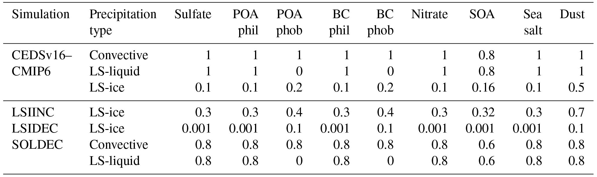
Additional model runs are performed to investigate the importance of differences in key processes for the aerosol distributions and model performance (Table 1). In addition to the CEDSv16 emissions, the model is run with ECLIPSEv5 and RCP4.5 emission inventories for anthropogenic emissions and GFED4 biomass burning emissions. Additionally, we perform simulations with ∘ (denoted 1×1) horizontal resolution. To investigate the importance of meteorology, the simulation with CEDSv16 emissions is repeated with meteorological data for the year 2000 instead of 2010. The year 2000 is selected due to its opposite El Niño–Southern Oscillation (ENSO) index compared to 2010. Finally, three model runs are performed with increased and decreased aerosol removal by large-scale ice clouds and decreased aerosol scavenging by liquid (large-scale and convective) precipitation. To modify the scavenging, we tune the fixed fractions that control aerosol removal efficiency in the model (see Sect. 2.1). Table 2 summarizes fractions used in the baseline configuration and the three sensitivity tests. A decrease and increase in efficiency of 0.2 is adopted for scavenging of all aerosols by liquid clouds (except hydrophobic BC and POA) and ice clouds, respectively. Note that there is no test with increased removal by liquid clouds, as, with the exception of hydrophobic BC, POA, and SOA, 100 % efficiency is already assumed. For ice clouds we also reduce the efficiency to a fraction of 0.1, or 0.001 if the value is 0.1 in the baseline configuration. We note that these changes do not represent realistic uncertainty ranges based on experimental or observational evidence, as there are limited constraints in the literature, but are chosen to explore the impact of a spread in the efficiency with which aerosols act as ice and cloud condensation nuclei.
2.4 Radiative transfer
We calculate the instantaneous top-of-the-atmosphere RF of anthropogenic aerosols due to aerosol–radiation interactions (RFari) (Myhre et al., 2013b). The radiative transfer calculations are performed offline with a multi-stream model using the discrete ordinate method (Stamnes et al., 1988). The model includes gas absorption, Rayleigh scattering, absorption and scattering by aerosols, and scattering by clouds. The RFari of individual aerosols is obtained by separate simulations, in which the concentration of the respective species is set to the preindustrial level. The aerosol optical properties have been updated from earlier calculations using this radiative transfer model (Myhre et al., 2007, 2009), in particular those associated with aerosol absorption. The Bond and Bergstrom (2006) recommendation of a mass absorption coefficient (MAC) for BC of around 7.5 m2 g−1 for freshly emitted BC and an enhancement factor of 1.5 for aged BC was used previously. In the present analysis, we apply a parametrization of MAC from observations over Europe by Zanatta et al. (2016), in which MAC depends on the ratio of non-BC to BC abundance. The mean MAC of BC from these observations around 10 m2 g−1 at 630 nm (Zanatta et al., 2016). The measurements in Zanatta et al. (2016) represent continental European levels. For very low concentrations of BC, the formula given in Zanatta et al. (2016) provides very high MAC values. We have therefore set a minimum level of BC of g m−3 for using this parameterization, and for lower concentrations we use Bond and Bergstrom (2006). In addition, we have set a maximum value of MAC of 15 m2 g−1 (637 nm) to avoid unrealistically high values of MAC compared to observed values. Organic matter has a large variation in the degree of absorption (e.g., Kirchstetter et al., 2004; Xie et al., 2017), from almost no absorption to a strong absorption in the ultraviolet region. Here, we have implemented absorbing organic matter according to refractive indices from Kirchstetter et al. (2004). The degree of absorption varies by source and region and is at present inadequately quantified: here we assume one-third of the biofuel organic matter and one-half of the SOA from anthropogenic volatile organic carbon (VOC) precursors. The remaining fractions of biofuel, fossil fuel, and marine POA and SOA (anthropogenic and all natural VOCs) are assumed to be purely scattering organic matter. As these fractions are not sufficiently constrained by observational data and associated with significant uncertainty, we also perform calculations with no absorption by organic matter for comparison.
2.5 Observations
A range of observational datasets are used to evaluate the model performance in the baseline simulation. Note that we use the term “black carbon” in a qualitative manner throughout the paper to refer to light-absorbing carbonaceous aerosols. However, when comparing with measurements, we use either elemental carbon (EC) or refractive BC (rBC), depending on whether the data are derived from methods specific to the carbon content of carbonaceous aerosols or incandescence methods, in line with recommendations from Petzold et al. (2013).
Measured surface concentrations of EC, OC, sulfate, and nitrate are obtained from various networks. For the US, measurements from IMPROVE (Interagency Monitoring of Protected Visual Environments) and CASTNET (Clean Air Status and Trends Network) are used. For Europe, data from EMEP (European Monitoring and Evaluation Programme) (Tørseth et al., 2012) and ACTRIS (Aerosols, Clouds and Trace gases Research InfraStructure) (Cavalli et al., 2016; Putaud et al., 2010) are used. EMEP and ACTRIS sites are all regional background sites, representative for a larger area. To broaden the geographical coverage we also compare the model output against additional observations from the Chinese Meteorological Administration Atmospheric Watch Network (CAWNET) in China (Zhang et al., 2012) and those reported in the literature from India (see Kumar et al., 2015, for more details). CASTNET, IMPROVE, EMEP, and ACTRIS data are from the year 2010, while CAWNET observations were sampled in 2006–2007, and the observational database from India compiled by Kumar et al. (2015) covers a range of years. IMPROVE provides mass of aerosols using filter analysis of measurements of particulate matter with a diameter of less than 2.5 µm (PM2.5), while CASTNET uses an open-face filter pack system with no size restriction to measure concentrations of atmospheric sulfur and nitrogen species (Lavery et al., 2009). Mass of individual species from the CAWNET network is obtained from aerosol chemical composition analysis performed on PM10 samples (Zhang et al., 2012). EMEP and ACTRIS measurements of EC and OC are in the PM2.5 range, whereas nitrate and sulfate measurements are filter based with no size cutoff limit. Data resulting from EMEP and ACTRIS are archived in the EBAS database (http://ebas.nilu.no, last access: April 2018) at NILU – Norwegian Institute for Air Research, and are openly available (see also the “Data availability” section).
Modeled AOD is evaluated against the Aerosol Robotic Network (AERONET). AERONET is a global network of stations measuring radiance at a range of wavelengths with ground-based sun photometers, from which aerosol column burden and optical properties can be retrieved (Dubovik and King, 2000; Holben et al., 1998). The comparison with AERONET data was carried out using the validation tools available from the AeroCom database hosted by Met Norway (http://aerocom.met.no/data.html, last access: March 2018). We also compare against AOD retrievals from MODIS-Aqua and MODIS-Terra (level 3 atmosphere products, AOD550 combined dark target and deep blue, product version 6) (MOD08, 2018) and the Multi-angle Imaging SpectroRadiometer (MISR) (level 2 aerosol product, product version 4) (Garay et al., 2018).
Table 3Global annual mean aerosol burdens (mg m−2) and total AOD in the baseline and sensitivity simulations. Parentheses in the top row give the atmospheric residence time (ratio of burden to total wet plus dry scavenging) (days). Corresponding values for the sensitivity simulations are given in Table S3. Results from the baseline CEDSv16–CMIP6 simulation are shown in bold.

* SOA is 1.1 mg m−2 (5.8 days) and POA is 2.3 mg m−2 (5.1 days).
Figure S1 in the Supplement depicts the locations of all the stations. For comparison with surface concentrations and AERONET AOD, the model data are linearly interpolated to the location of each station using annual mean, monthly mean (concentrations), or 3-hourly output (AOD), depending on the resolution of the observations. In the case of AERONET, high mountain stations (here defined as having an elevation higher than 1000 m above sea level) are excluded following Kinne et al. (2013). For comparison with observed OC surface concentrations, modeled OA is converted to OC using factor of 1.6 for POA and 1.8 for SOA. Unless measurements are restricted to the PM2.5 size range, the comparison includes both fine- and coarse-mode modeled nitrate (Sect. 2.1). Several statistical metrics are used to assess the model skill, including correlation coefficient (R), root-mean-square error (RMSE), variance, and normalized mean bias (NMB).
The modeled vertical distribution of BC is compared with aircraft measurements of refractory BC (rBC) from the HIAPER Pole-to-Pole Observations (HIPPO) campaign (Wofsy et al., 2011). Vertical profiles of BC from Oslo CTM2 have been evaluated in several previous studies (e.g., Samset et al., 2014) and a more thorough comparison of Oslo CTM3 results against a broader set of campaigns is provided by Lund et al. (2018). In the present analysis we focus on data from the third phase (HIPPO3) flights, the only phase that was conducted in 2010, i.e., the same year as our sensitivity simulations. Model data are extracted along the flight track using an online flight simulator. The data are separated into five latitude regions and vertical profiles constructed by averaging observations and model output in 13 altitude bins.
We first document the aerosol distributions simulated in the baseline model configuration, focusing on the anthropogenic contribution, and compare with observations, multi-model studies, and results from the sensitivity tests. With the present-day model performance evaluated, we then present the updated historical development of RFari of anthropogenic aerosols.
3.1 Evaluation of present-day aerosol distributions
The global mean aerosol burdens and atmospheric residence times (ratio of burden to total wet plus dry deposition) in the baseline simulation are summarized in Table 3 (top row), with spatial distribution shown in Fig. S2. Compared to results from the AeroCom III experiment, the Oslo CTM3 sulfate burden of 5.4 mg m−2 estimated here is about 50 % higher than the multi-model mean of 3.5 mg m−2 and 35 % higher than Oslo CTM2 (Bian et al., 2017). While the total SO2 emission is only 5 % higher in the present study than in the Oslo CTM2 AeroCom III simulation, the atmospheric residence time of sulfate is 50 % longer, suggesting that the burden difference is mainly attributable to changes in the parameterization of dry and large-scale wet deposition in Oslo CTM3 (Sect. 2.1). The nitrate burden is nearly a factor of 3 higher than both the AeroCom multi-model mean and Oslo CTM2 burden and higher than all nine models contributing in AeroCom III (Bian et al., 2017). This is mainly due to a higher burden of coarse-mode nitrate aerosols, associated with less-efficient scavenging of sea salt in Oslo CTM3 than Oslo CTM2. The global budgets of OA simulated by the AeroCom II models were analyzed by Tsigaridis et al. (2014). The burden of OA in Oslo CTM3 of 3.4 mg m−2 is close to their multi-model mean of 3.1 mg m−2 and 25 % higher than that in Oslo CTM2. The Oslo CTM3 estimate includes the contribution from marine OA emissions (Sect. 2.1), which may explain part of the difference as marine OA was included in some of the AeroCom II models, but not Oslo CTM2. However, the marine POA only contributes around 3 % to the total OA. Additionally, the residence time of OA of 5.3 days is longer than in the Oslo CTM2 AeroCom II experiment. The global BC burden of 0.23 mg m−2 is also close to the mean of the AeroCom II models of 0.25 mg m−2 (Samset et al., 2014). We note that different emission inventories were used in the AeroCom experiments and the present analysis; however, the comparison shows that the aerosol burdens simulated by Oslo CTM3 fall within the range of existing estimates from global models.
Figure 1 shows results from the baseline Oslo CTM3 simulation against annual mean measured surface concentrations of EC, OC, sulfate, and nitrate in Europe, North America, and Asia. Overall, Oslo CTM3 shows a high correlation of 0.8–0.9 with measured surface concentrations. There is a general tendency of underestimation by the model, with the lowest NMB and RMSE for BC and nitrate (−23 %) and the highest for sulfate (−51 %). There are, however, notable differences in model performance among datasets in different regions, as seen from Table S2. For all species, the NMB and RMSE are highest for measurements in China. For instance, excluding the CAWNET measurements reduces the NMB for sulfate in Fig. 1 from −51 % to −31 % (not shown). In contrast, the correlation with CAWNET observations is generally similar to, or higher than, other regions and networks. In the case of BC and nitrate, the model slightly overestimates concentrations in Europe and North America, but underestimates Asian measurements. The best overall agreement is generally with IMPROVE observations in North America. Differences in instrumentation among different networks can affect the evaluation. Lavery et al. (2009) found that measurements from CASTNET typically gave higher nitrate surface concentrations than values obtained from co-located IMPROVE stations, which could partly explain the NMB of opposite sign in these two networks in Table S2. For BC, we also include measurements from across India compiled by Kumar et al. (2015). This is a region where emissions have increased strongly, but where evaluation of the model performance so far has been limited due to availability of observations. The model underestimates concentrations with a NMB of −43 %; however, the correlation of 0.60 is similar to the comparison with data from China and higher than the other regions. An examination of the monthly concentrations (Fig. S3) shows that the largest discrepancies occur during winter, with the largest bias found for measurements in northeast India. One possible reason could be missing or underestimated emission sources. This finding is similar to the comparison of measurements against WRF-Chem by Kumar et al. (2015). The seasonality of BC concentrations has also been an issue at high northern latitudes, where earlier versions of Oslo CTM strongly underestimated winter and springtime surface concentrations at Arctic stations (Lund et al., 2017; Skeie et al., 2011), similar to many other models (Eckhardt et al., 2015). This Arctic underestimation persists in the current version of the model. Seasonal differences also exist in other regions, but not consistently across measurement networks. Compared with EC measurements from EMEP–ACTRIS the correlation is poorer during winter and spring, and the model underestimates concentrations in contrast to a positive NMB in summer and fall. However, due to the relatively low number of stations, these values are sensitive to a few stations with larger measurement–model discrepancies. For both IMPROVE and EMEP–ACTRIS, the model underestimation of sulfate is larger during summer and fall, but with opposite seasonal differences in correlation. In general, the number of stations and evaluation of data from only 1 year limit the analysis of seasonal variations.
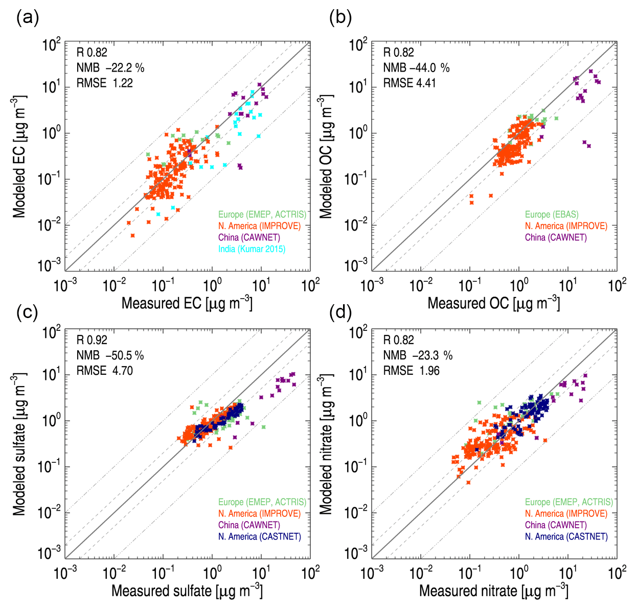
Figure 1Annual mean modeled versus measured aerosol surface concentrations of (a) EC, (b) OC, (c) sulfate, and (d) nitrate from the IMPROVE, EMEP, ACTRIS, CASTNET, and CAWNET measurement networks.
We do not evaluate ammonium concentrations in the present analysis, as that requires a detailed discussion of the nitrate and sulfate budgets, which has been covered by the recent multi-model evaluation by Bian et al. (2017) based on an AeroCom Phase III experiment, in which Oslo CTM3 participated. Results showed that most models tend to underestimate ammonium concentrations compared to observations in North America, Europe, and East Asia, with a multi-model mean bias and correlation of 0.88 and 0.47, respectively. Oslo CTM3 shows good agreement with ammonium measurements in North America but has a bias and correlation close to the model average in the other two regions.
In May 2017, after completion of our historical simulations, an updated version of the CEDS emission inventory was released after an error in the code was reported (see Sect. 2.2). This resulted in occasional shifts in the spatial distribution of emissions within countries with a large spatial extent (e.g., USA and China). Since the emission totals were not affected, the impact on our RFari estimates is likely to be small, but shifts in the emission distribution could influence the model evaluation, in particular for surface concentrations. While repeating all simulations would require more resources, we have repeated the year 2010 and 1750 runs. Figure S4 shows the comparison of modeled concentrations against IMPROVE measurements with the two emission inventory versions, CEDSv16 and CEDSv17. In the case of BC, the comparison shows a 5 % higher correlation and 15 % lower RMSE with CEDSv17 than with CEDSv16. A similar improvement is found for nitrate, with 26 % higher correlation and 12 % lower RMSE, while in the case of OC and sulfate, the difference is small (<5 %). Smaller differences of between 2 % and 10 % are also found in the comparison against measurements in Europe and Asia (not shown). Hence, using the updated version of the emission inventory has an effect on the model performance in terms of surface concentrations, but without changing the overall features or conclusions. The net RFari in 2010 relative to 1750 is 2 % stronger with the CEDSv17 inventory, a combined effect of slightly higher global BC burden and lower burdens of sulfate and OA.
As shown in Table S2, the model overestimates surface concentrations in some regions and underestimates them in others. Compensating biases can influence the evaluation of total AOD. Moreover, the biases differ in magnitude among different species. Moving one step further, we therefore examine the average aerosol composition in the three regions where this is possible with our available measurements. Figure 2 shows the relative contribution from different aerosol species to the total mass in the IMPROVE, EMEP–ACTRIS, and CAWNET measurements and the corresponding model results. The number of available aerosol species varies among the measurement networks and we include sea salt from IMPROVE and ammonium from CAWNET. Additionally, the number of stations at which simultaneous measurements of all species were available also differs substantially, with 16 for CAWNET, five for EMEP–ACTRIS and 172 for IMPROVE. Overall, the relative composition is well represented by the model. The agreement is particularly good for the IMPROVE network. Compared to measurements from CAWNET, the model has a lower relative contribution from OC and more sulfate. In the case of Europe, nitrate aerosols also constitute a significantly larger fraction in the model than in the observations. The evaluation of nitrate is complicated by possible differences in the detection range of instrumentation compared to the size of the two nitrate modes in the model (Sect. 2.1). The comparison against EMEP nitrate data includes both coarse- and fine-mode modeled nitrate. Excluding the coarse mode, the fraction of total mass attributable to nitrate decreases from 43 % to 28 %, which is much closer to the observed 30 % contribution. However, this affects the comparison in Fig. 1, resulting in a negative NMB of −34 %, compared to −23 % when including both coarse and fine modes. This suggests that part, but not all, of the nitrate represented as a coarse mode in the model is measured by the instrument, pointing to a need for a more sophisticated size distribution in the model to make better use of available observations. The low number of available stations from EMEP–ACTRIS could also be an important factor.
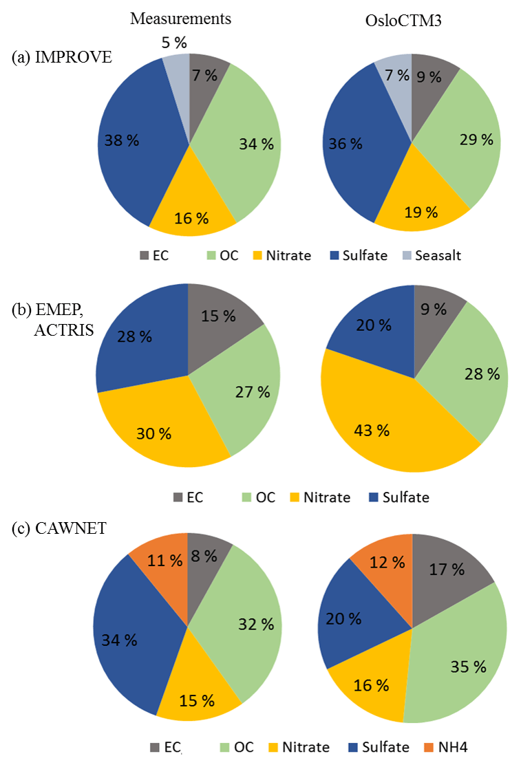
Figure 2Aerosol composition (fraction of total aerosol mass) derived from the IMPROVE, EMEP–ACTRIS, and CAWNET networks (left column) and corresponding Oslo CTM3 results (right column).
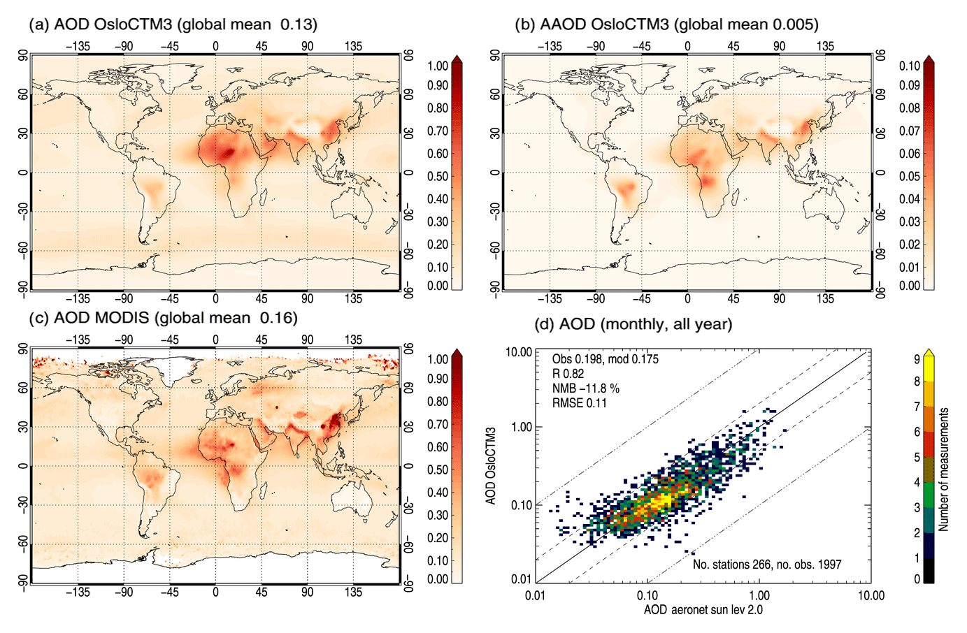
Figure 3Annual mean (year 2010) modeled (a) AOD and (b) AAOD, (c) MODIS-Aqua AOD retrieval, and (d) scatter density plot of the comparison of simulated AOD against monthly mean AERONET observations.
Next, we examine total AOD. Figure 3 shows modeled AOD and aerosol absorption optical depth (AAOD), AOD retrieved from MODIS-Aqua, and a comparison of modeled AOD with AERONET observations. Modeled global annual mean AOD and AAOD is 0.13 (Fig. 3a) and 0.005 (Fig. 3b), respectively. The overall spatial pattern of modeled AOD agrees well with MODIS (Fig. 3c); however, the latter gives a higher global mean of 0.16 and clearly higher values in north India and parts of China, as well as central Africa. These peak values are similar to those of MODIS-Terra but less pronounced in the AOD retrieved from MISR (Fig. S5), illustrating important differences among different remote-sensing products. Nevertheless, an underestimation of modeled AOD in Asia is consistent with results from the evaluation of surface concentrations and can also be seen in the comparison against AERONET, as discussed below. Oslo CTM3 shows a good agreement with measured AOD from the AERONET network, with an overall correlation of 0.82 and RMSE of 0.11, when using monthly mean data from 266 stations (Fig. 3d). Note that the modeled global mean AOD is 0.13, but the model mean at the AERONET stations is 0.175 (Fig. 3d) and has a NMB of only −11.8 %. Many of the AERONET stations tend not to be regional background sites, but can be influenced by local pollution (e.g., Wang et al., 2018).
There are notable regional differences in model performance. Figure S6 compares modeled AOD against AERONET stations in Europe, North America, India, and China separately. The best agreement is found for Europe and North America, with a NMB of −0.4 % and −13 %, respectively, and RMSE of approximately 0.05. The correlation is higher for North America (0.76) than Europe (0.63). A relatively high correlation of 0.71 is also found for stations in China. However, the NMB and RMSE are higher (−34 % and 0.25). There are significantly fewer observations for comparison with modeled AOD over India, but the ones available give NMB and RMSE on the same order of magnitude as for China, but a lower correlation (0.45).
Ground-based measurements can also provide information about column AAOD. Such information has been used to constrain the absorption of BC and provide top-down estimates of the direct BC RF (e.g., Bond et al., 2013). However, retrieval and application of AERONET AAOD is associated with a number of challenges and uncertainties (e.g., Samset et al., 2018); hence such an evaluation is not performed here.
Recent literature has pointed to important representativeness errors arising when observations are used to constrain models due to the coarse spatial and temporal scales of global models compared with the heterogeneity of observations. Schutgens et al. (2016a) found differences in RMSE of up to 100 % for aerosol optical thickness when aggregating high-resolution model output over grid boxes representative of the resolution of current global models compared to small areas corresponding to satellite pixels. Smaller, but notable, differences of up to 20 % were found when monthly mean model data were used, as in the present analysis. However, that did not account for issues related to temporal collocation, which can also introduce considerable errors (Schutgens et al., 2016b). In a recent study, Wang et al. (2018) found a spatial representativeness error of 30 % when constraining AAOD modeled at a horizontal resolution against AERONET retrievals. However, further work is needed to investigate whether similar biases exist for AOD.
3.2 Sensitivity of aerosol distributions to model input and process parameterization
As shown in the section above, Oslo CTM3 performs well compared against observed AOD. Still, a number of factors influence the simulated distributions of individual aerosol species. To assess the importance of key uncertainties for modeled distributions and model performance, we perform a range of sensitivity simulations (Table 1) to examine the importance of emission inventory, scavenging assumptions (Table 2), meteorological data, and resolution for the modeled aerosol distributions and model performance.
Global aerosol burdens and AOD in each sensitivity run are summarized in Table 3 (corresponding atmospheric residence times are given in Table S3). The BC burden is particularly sensitive to reduced scavenging by large-scale ice clouds (LSIDEC), resulting in a 40 % higher burden compared to the baseline. In contrast, an equal increase in the scavenging efficiency (LSIINC) results in a decrease in burden of only 9 %, while decreased scavenging by liquid precipitation (SOLDEC) gives a 13 % higher burden. The lower BC emissions in the ECLv5 and CMIP5 inventories give a global BC burden that is 9 % and 22 % lower, respectively. For sulfate, ammonium, and OA, we also find the largest burden changes in the LSIDEC case, followed by SOLDEC. The change in the LSIDEC case is particularly large for OA and is driven by changes in SOA. For SOA, the changes are determined not only by modifying the scavenging, but also by changes in POA concentrations, onto which gas-phase secondary organics can partition. Increasing the horizontal resolution results in a slightly higher burden for all species, except sea salt.
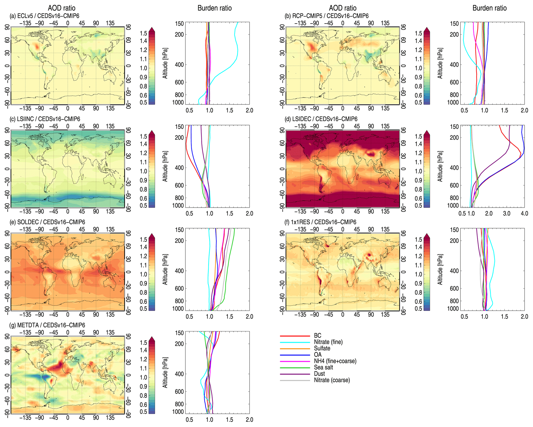
Figure 4Ratio of each sensitivity simulation relative to the baseline for AOD (columns 1 and 3) and total burden by species in each model layer (columns 2 and 4).
While sensitivity tests may give similar changes in the total global burdens, the spatial distribution of changes can differ substantially. Figure 4 shows the ratio of AOD and total burden by species and altitude in each sensitivity simulation to the baseline. As expected, varying the emission inventories results in changes that are largely confined to the main source regions (Fig. 4a, b). Using the CMIP5 inventory results in considerably lower concentrations over Asia, the Middle East, and North Africa, reflecting the higher emissions in the more recent inventory. Over central North America the AOD is higher, mainly due to more ammonium nitrate, whereas the higher AOD over eastern Europe and part of Russia is a result of higher sulfate concentrations. Similar characteristics are found when using ECLv5, but the relative differences are smaller. Reducing or increasing the large-scale ice cloud scavenging gives the largest relative changes in AOD at high latitudes, while changes in the solubility assumption for liquid precipitation affect AOD most over Asia, where aerosol burdens are high, and around the Equator where convective activity is strong. In general, the burden of BC, OA, and dust is significantly affected by changes in the scavenging assumptions, while nitrate responds more strongly to different emission inventories, likely due to the complicated dependence on emissions of several precursors and competition with ammonium sulfate. We also note that at higher altitudes the absolute differences in the burden of nitrate are small. Changes in AOD resulting from using different meteorological input data are more heterogeneous and are most notable in regions where effects of choosing data from years with an opposite ENSO phase are expected, e.g., the west coast of South America and Southeast Asia. There is also a notable change in the Atlantic Ocean, where mineral dust is a dominating species. The meteorological data can affect production, deposition, and transport of dust directly as well as indirectly through ENSO-induced teleconnections as suggested by Parhi et al. (2016), for example.
For BC, OA, and dust, the largest impacts relative to the baseline are seen above 600 hPa in the LSIDEC case. Changes in LSIDEC are also important in the case of sulfate and sea salt but occur at lower altitudes. In contrast to the other aerosol species, differences in emission inventories are most important for nitrate. In a recent study, Kipling et al. (2016) investigated factors controlling the vertical distribution of aerosols in the HadGEM3–UKCA. It was found that in-cloud scavenging was very important in controlling the vertical mass concentration of all species, except dust. For dust, it was also found that dry deposition and sub-cloud processes played key roles, processes not examined in the present analysis. Moreover, Kipling et al. (2016) performed sensitivity simulations by switching transport and scavenging on and off to get the full effect of a given process, while we perform smaller perturbations to investigate uncertainties. Here we find significant impacts of changes in ice cloud removal efficiency (Table 2) on the vertical distribution of BC, OA, and dust, while large-scale liquid and convective precipitation is more important for sea salt and nitrate
Our sensitivity tests show that changes in input data, resolution, or scavenging can lead to notable changes in the aerosol distributions. The next question is then how these changes affect model performance compared to observations. Figure 5a compares modeled and measured surface concentrations of BC, OC, sulfate, and nitrate in each simulation using all observations in Fig. S1. For BC, the sensitivity tests have little or no impact on correlation, but there is a markedly better agreement in terms of standard deviation (i.e., model becomes closer to observations) for CEDSv16–CMIP6 compared to RCP–CMIP5, reflecting the higher emissions in the former. Similar, but smaller, effects are also found for the other species. The improvement from RCP–CMIP5 to CEDSv16–CMIP6 is especially seen for measurements in Asia. A higher resolution is also found to reduce the bias, in particular for BC. Figure 5b shows the comparison against AERONET AOD in each sensitivity simulation. Again, there is a higher correlation and lower bias in the 1x1RES run than in the baseline, while the opposite is found in the RCP–CMIP5 and ECLv5 cases. For both observables, the improvement in the 1x1RES simulation may result from a better sampling at a finer resolution, improved spatial distribution, or a combination of both. The most pronounced changes result from using meteorological data from the year 2000, in which case the correlation is reduced from around 0.8 to 0.7.
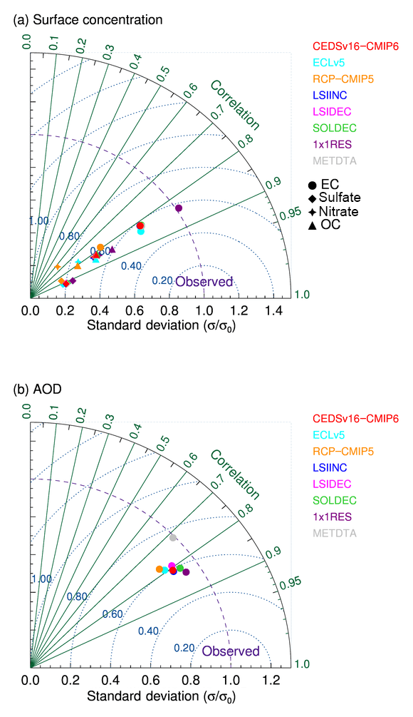
Figure 5Taylor diagram of modeled and measured aerosol surface concentrations in the baseline simulation and sensitivity tests using all observations in Fig. 1.
For both observables, the difference in model performance between the baseline and scavenging sensitivity tests is small. This may partly be an effect of the geographical coverage of stations; the majority of measurements are from stations in more urban regions, whereas simulated burden changes occur in remote regions, particularly at high latitudes and altitudes (Fig. 4). We therefore also perform evaluations against AOD from regional subsets of AERONET stations. A total of 10 of the AERONET stations used in the present analysis are located north of 65∘ N (Fig. S1). A comparison of monthly mean simulated AOD in each of the sensitivity runs against observations in this region shows the best agreement with the baseline simulation and with the ECLv5 emission inventory, with a considerably higher bias when scavenging parameters are modified (Fig. S7a). This is particularly the case in the LSIDEC run, in which concentrations of all species increase at high latitudes compared to the baseline (Fig. 4). In contrast, the reduced concentrations in LSIINC result in a negative bias. We note that most of these stations have missing values in the winter months, which is when the model underestimates BC concentrations in the Arctic, hence limiting the evaluation. Decreased scavenging efficiency also leads to a higher bias than in the baseline for observations in Europe and North America (not shown). In Asia, where the model already underestimates aerosols in the baseline configuration, the bias is reduced since concentrations increase. However, differences are smaller than north of 65∘ N. Moreover, given the notable exacerbation in model performance in other regions, it is likely that other sources of uncertainty (e.g., emissions) are more important for the model–measurement discrepancies in Asia. A similar comparison is performed for 15 AERONET stations located in North Africa and the Middle East (Fig. S7b), where the dust influence is strong. Changing the meteorological year and reducing scavenging results in higher dust burdens (Table 3). Again, the agreement is better in the baseline run than in these sensitivity runs. In particular, the METDATA run results in a higher bias and a lower correlation, which is not surprising as dust production also depends on meteorological conditions. The changes compared to the baseline CEDSv16–CMIP6 simulation cannot be entirely attributed to differences in dust concentrations, as seen from the RCP–CMIP5 and ECLv5 simulations in which the dust production is equal to the baseline. Several studies have pointed to the importance of spatial resolution for improved model performance compared to observations (e.g., Sato et al., 2016; Schutgens et al., 2017, 2016a; Wang et al., 2016). Wang et al. (2016) found significant reductions in NMB of BC AAOD relative to AERONET when using high-resolution (10 km) emission data and model output. In our analysis, moving from to horizontal resolution also results in a slightly higher correlation and reduced bias and errors when compared to all AERONET stations (Fig. 5b). The impact is largest for AOD in China and India: the NMB is reduced (from −34 % and −24 % (Fig. S6) to −20 % and −10 %, respectively). However, the opposite effect is found for AERONET stations in Europe and North America. Of course, the resolution is still very coarse compared to the grid sizes used in the abovementioned studies.
Changes away from near-source areas are also evaluated in terms of BC concentrations by a comparison with observed vertical distribution from the HIPPO3 campaign, in which remote marine air over the Pacific was sampled across all latitudes (Sect. 2.5). To limit the number of model runs, we focus on only one phase of the HIPPO campaign here, but a more comprehensive evaluation of Oslo CTM3 vertical BC distribution against aircraft measurements was performed by Lund et al. (2018). Figure 6 shows observed average vertical BC concentration profiles against model results from each sensitivity test. Oslo CTM3 reproduces the vertical distribution well in low latitudes and midlatitudes over the Pacific in its baseline configuration, although near-surface concentrations in the tropics are underestimated. This is a significant improvement over Oslo CTM2, for which high-altitude concentrations in these regions were typically overestimated. The baseline configuration of Oslo CTM3 includes updates to the scavenging assumptions based on previous studies investigating reasons for the high-altitude discrepancies (e.g., Hodnebrog et al., 2014; Lund et al., 2017). At high northern and southern latitudes, the model underestimates the observed vertical profiles in the baseline. Increasing the model resolution does not have any notable impact on the vertical profiles. There is a notable increase in high-latitude concentrations when large-scale ice cloud scavenging is decreased. However, there is a simultaneous exacerbation of model performance in the other latitude bands, pointing to potential tradeoffs when tuning global parameters, as also illustrated by Lund et al. (2017). Due to the significant altitude dependence of the radiative effect of BC (e.g., Samset et al., 2013), high-altitude overestimations will contribute to uncertainties in BC RFari. We also note that HIPPO3 was conducted in March–April: comparison with aircraft measurements from other seasons shows a smaller underestimation at high latitudes (Lund et al., 2018).

Figure 6Modeled vertical BC profiles against rBC aircraft measurements in five different latitude bands over the Pacific Ocean from the HIPPO3 flight campaign. Model data are extracted along the flight track using an online flight simulator. Black lines show the mean of observations (solid), mean + plus 1 standard deviation (dashed). Colored lines show the Oslo CTM3 baseline (CEDSv16–CMIP6) (solid) and sensitivity simulations (dashed).
3.3 Preindustrial to present-day aerosols
With confidence in the model ability to reasonably represent current aerosol distributions established, we next present an updated historical evolution of anthropogenic aerosols, and the consequent direct radiative effect, from the preindustrial era to present day (RFari) (Sect. 2.4). Figure 7 shows the net change in total aerosol load from 1750 to 2014. Full times series by species are given in Table S4. To keep in line with the terminology used in the IPCC AR5, we now separate out biomass burning BC and POA in a separate species “biomass”. We also note that only the fine-mode fraction of nitrate contributes to the RFari and is included in Fig. 7. To illustrate the contributions from additional emissions during the past 14 years, we also include the 2000–1750 difference. The values from the present study are also compared with results from the AeroCom II models (Myhre et al., 2013a), in which emissions over the period from 1850 to 2000 from Lamarque et al. (2010) were used.

Figure 7Change in anthropogenic aerosol load over the period from 1750 to 2014 using CEDSv16 emissions. Black symbols show the 1750 to 2000 difference and red symbols show multi-model mean and Oslo CTM2 results from the AeroCom II experiments (Myhre et al., 2013a).
The most notable difference compared to the AeroCom II results is seen for biomass aerosols. Biomass burning emissions have high interannual variability and this affects the analysis. While the 1750–2014 difference is 0.23 mg m−2, taking the difference between the years 1750 and 2000 (black triangle) results in a net change of only 0.03 mg m−2. There is also a much larger change in the burden of biomass aerosols in the AeroCom experiments, reflecting more than 100 % higher emissions in 2000 compared to in the 1850 (Lamarque et al., 2010) inventory. However, biomass aerosols comprise both scattering OA and absorbing BC and, as seen below, these nearly cancel out in terms of RFari. Changes in sulfate and OA from the preindustrial era to 2000 are slightly higher in the present analysis than in AeroCom II, and the influence of additional emissions since 2000 is seen. Oslo CTM3 is well below the AeroCom multi-model mean for nitrate. Oslo CTM2 was found to be in the low range, but the multi-model mean was also influenced by some models giving high estimates (Myhre et al., 2013a).

Figure 8(a) Time evolution of RFari. Solid lines show Oslo CTM3 results from the current study, while dashed lines show results from IPCC AR5 (Myhre et al., 2013b). The inset shows the change in total RFari between 1990 and 2015 in the current study compared with IPCC AR5 and multi-model mean and Oslo CTM2 results from Myhre et al. (2017) using ECLv5 emissions. (b) Zonal mean RFari 1750–2014.
Using the CEDSv16 emissions, we estimate net RFari from all anthropogenic aerosols in 2014 relative to 1750 of −0.17 W m−2. The RFari from sulfate is −0.30 W m−2, while the contributions from OA (combined fossil fuel plus biofuel POA and SOA), nitrate, and biomass aerosols are smaller with a magnitude of −0.09, −0.02, and −0.0004 W m−2, respectively. The RFari due to fossil fuel and biofuel BC over the period is 0.31 W m−2.
Figure 8a shows the time series of RFari by component, as well as the net RFari, in the present analysis (solid lines), and corresponding results from the IPCC AR5 (dashed lines). The net RFari over time is mainly determined by the relative importance of compensating for BC and sulfate RFari. The most rapid increase in BC RFari is seen between 1950 and 1990, as emissions in Asia started to grow, outweighing reductions in North America and Europe (Hoesly et al., 2018). After a period of little change between 1990 and 2000, the rate of change increases again over the past 2 decades, following strong emission increases in Asia and South Africa. Similarly, the cooling contribution from sulfate aerosols strengthened from around mid-century. However, in contrast to BC, the evolution is fairly flat after 1990. The last 20 years has seen a continuous reduction in sulfur dioxide (SO2) emissions in Europe, from around 30 to 5 Tg yr−1 in CEDSv16, with a similar trend in North America. While emissions in China continue to increase well into the 2000s, a stabilization is seen after 2010, following introduction of stricter emission limits as part of a program to desulfurize power plants (Klimont et al., 2013). During the same period, emissions in India have risen. However, the net global SO2 emission trend over the past few years is a slight decline (Hoesly et al., 2018). This development is reflected in the net RFari, which reaches its peak (i.e., strongest negative value) around 1990 and gradually becomes weaker thereafter. This trend is more pronounced in the present analysis than in the IPCC AR5 estimates, in which the forcing due to sulfate is more flat in recent decades, suggesting that projected emission estimates underestimated recent decreases in SO2. The minimum net RFari value is also reached later in the latter. Moreover, a recent study suggests that current inventories underestimate the decline in Chinese SO2 emissions and estimate a 75 % reduction since 2007 (Li et al., 2017). In this case, the weakening trend could be even stronger than estimated here. The insert in Fig. 8a focuses on recent estimates of total RFari over the period of 1990–2015. Using the ECLv5 emission inventory, Myhre et al. (2017) found a global mean RFari due to changes in aerosol abundances over the period of 1990–2015 of 0.05(±0.04) W m−2. Our results using CEDSv16 emissions are in close agreement with these findings.
Over the past decades, there has been a shift in emissions, from North America and Europe to South and East Asia. This is also reflected in the zonally averaged net RFari over time in Fig. 8b. RFari declined in magnitude north of 40∘ N after 1980, with particularly large year-to-year decreases between 1990 and 1995, and from 2005 to 2010 and strengthened in magnitude between 10 and 30∘ N. The RFari also strengthened in the Southern Hemisphere subtropical region, reflecting increasing emissions in Africa and South America after 1970. However, the peak net RFari is considerably weaker in 2014 than the peak in 1980. This is mainly due to the fact that simultaneously with the southwards shift, the sulfate burden has declined, while the BC burden has increased steadily at the same latitudes, resulting in a weaker net RF. Over the past decade, the net RFari has switched from negative to positive north of 70∘ N, due to a combination of stronger positive RF of BC and biomass burning aerosols.
Table S5 shows changes in burden, AOD, AAOD, RFari, and normalized RF over the period of 1750–2010 for individual aerosol components and the net RFari. Compared to earlier versions of Oslo CTM (Myhre et al., 2009, 2013a), the normalized RF with respect to AOD is lower because of the short lifetime of BC resulting in a smaller abundance of BC above clouds, whereas normalized RF with burden is comparable to earlier estimates because a higher MAC compensates for the short lifetime of BC. Weaker normalized RF of OA (POA and SOA) than earlier Oslo CTM versions is due to the inclusion of absorbing OA.
In the present study we have used an updated parameterization of BC absorption based on Zanatta et al. (2016) (Sect. 2.4), which takes into account the ratio of non-BC to BC material and results in a MAC of 12.5 m2 g−1 at 550 nm. This is 26 % higher than 9.94 m2 g−1 using the approach from Bond and Bergstrom (2006). Using the latter, we estimate a BC RFari in 2014 relative to 1750 of 0.23 W m−2, 25 % lower than the 0.31 W m−2 calculated based on Zanatta et al. (2016). These results emphasize the importance of assumptions and uncertainties related to the BC absorption.
The magnitude of RFari by scattering aerosols is sensitive to assumptions about absorption by organic aerosols, so-called brown carbon (BrC). Observational studies have provided evidence for the existence of such particles, and modeling studies suggest they could be responsible for a substantial fraction of total aerosol absorption, although the spread in estimates is wide (e.g., Feng et al., 2013, and references therein). In the present study we assume a considerable fraction of absorption by OA (Sect. 2.4). Assuming purely scattering aerosols, the RFari from OA is −0.13 W m−2; accounting for BrC absorption, this is weakened to −0.09 W m−2. Splitting total OA RFari into contributions from primary and secondary aerosols, we find that purely scattering POA gives a RFari of −0.07 W m−2 compared to −0.06 W m−2 with absorption. The corresponding numbers for SOA are −0.06 and −0.03 W m−2. This indicates that in Oslo CTM3, the absorbing properties of SOA are relatively more important than for POA. This is likely due to the generally higher altitude of SOA than POA (Fig. S8) in combination with the increasing radiative efficiency of absorbing aerosols with altitude (Samset et al., 2013). However, due to the weaker overall contributions from OA, our results indicate that differences in parameterization of BC absorption can be more important than uncertainties in absorption by BrC for the net RFari.
Our estimate of total net RFari in 2014 relative to 1750 is weaker in magnitude than the best estimate for the 1750–2010 period reported by IPCC AR5. The difference is due to a combination of factors, including weaker contributions from both cooling aerosols and BC. Despite considerably higher BC emissions in the CEDSv16 inventory compared to older inventories, we calculate a weaker BC RFari than reported in AR5, hence going in the opposite direction of explaining the difference to IPCC AR5 total RFari. The IPCC AR5 best estimate for fossil fuel and biofuel BC of 0.4 (0.05 to 0.8) W m−2 (Boucher et al., 2013) was based mainly on the two studies by Myhre et al. (2013a) and Bond et al. (2013), who derived estimates of BC RFari of 0.23 (0.06 to 0.48) W m−2 and 0.51 (0.06 to 0.91) W m−2, respectively. The spread between the two is largely attributed to methodological differences: Bond et al. (2013) used an observationally weighted scaling of results to match those based on AERONET AAOD, which was not adopted by Myhre et al. (2013a). Such ad hoc adjustments typically result in higher estimates (Wang et al., 2018, and references therein). Moreover, a recent study by Wang et al. (2018) suggests that representativeness error arising when constraining coarse-resolution models with AERONET AAOD could result in a 30 % overestimation of BC RFari, which explains some of the differences between bottom-up and observationally constrained numbers. The BC RFari estimate from the present study is around 20 % higher than the AeroCom multi-model mean from Myhre et al. (2013a) when calculated over the same period of 1850–2000. This reflects the higher emissions in the CEDSv16 emission inventory than in Lamarque et al. (2010), as well as a higher MAC.
A significant range from −0.85 to +0.15 W m−2 surrounds the central RFari estimate of −0.35 W m−2 from IPCC AR5 (Boucher et al., 2013), caused by the large spread in underlying simulated aerosol distributions. Deficiencies in the ability of global models to reproduce atmospheric aerosol concentrations can propagate to uncertainties in RF estimates. As shown in Sect. 3, Oslo CTM3 generally lies close to or above the multi-model mean of anthropogenic aerosol burdens from recent studies and is found to perform reasonably well compared with observations and other global models, with improvements over the predecessor Oslo CTM2. In particular, recent progress towards constraining the vertical distribution of BC concentrations has resulted in improved agreement between modeled and observed vertical BC profiles over the Pacific Ocean with less of the high-altitude overestimation seen in earlier studies. However, as shown by Lund et al. (2018), there are discrepancies compared to recent aircraft measurements over the Atlantic Ocean. A remaining challenge is the model underestimation of Arctic BC concentrations. However, this is seen mainly during winter and early spring, when the direct aerosol effect is small due to lack of sunlight. In contrast, the higher emissions in the CEDSv16 inventory also result in an improved agreement with BC surface concentrations over Asia.
In general, we find lower surface sulfate concentrations in the model compared with measurements. This could contribute to an underestimation of the sulfate RFari, which is weaker in the present study than in IPCC AR5. An underestimation of observed AOD in Asia is also found; however, the implication of this bias on RF is not straightforward to assess, as it is complicated by the mix of absorbing and scattering aerosols. We note that the global mean sulfate burden is higher in Oslo CTM3 than in most of the global models participating in the AeroCom III experiment (Sect. 3.1, Bian et al., 2017) and that Oslo CTM3 performs similarly to or better than other AeroCom Phase III models in terms of nitrate and sulfate surface concentrations, at least for measurements from CASTNET (Bian et al., 2017). Nevertheless, the model diversity in simulated nitrate and sulfate remains large and, although all models capture the main observed features in concentrations, further work is needed to resolve the differences and improve model performance for these species.
While a comprehensive quantitative uncertainty analysis of the updated RFari estimate is not possible within the scope of this study, we explore the order of magnitude uncertainties due to “internal” factors such as scavenging parameterizations and model resolution by performing sensitivity tests. Changes in global burden on the order of 10 %–20 %, and up to 65 %, were found (Sect. 3.2). However, compared to observations of surface concentrations in near-source regions, total AOD, and vertical distribution of BC concentrations, we saw that the model generally performed the best in its baseline configuration. Furthermore, the largest changes in the simulated AOD and aerosol distributions were found in high-latitude regions, whereas changes over land where the concentrations, and hence subsequent RF, are localized were smaller. For certain regions and observations, there were notable differences between the baseline and sensitivity simulations. For instance, an improvement in the baseline compared to using the CMIP5 emission inventory was seen for BC surface concentrations, in particular in Asia, while the NMB of AOD compared to AERONET stations in the same region was reduced in the simulation with higher spatial resolution. The importance of using the correct meteorological year was also seen. Such uncertainties will translate to the RFari estimates, along with uncertainties in optical properties such as absorption by organic aerosols and parameterization of BC absorption (Sect. 3.3).
Estimates of radiative impacts depend critically on the confidence in the emission inventories. A detailed discussion of uncertainties in the CEDS inventory is provided by Hoesly et al. (2018). On a global level, the uncertainty in SO2 emissions tends to be relatively low, although there is an indication of missing SO2 sources in particular in the Persian Gulf (McLinden et al., 2016), whereas emission factors for BC, OC, NOx, CO, and VOCs have higher uncertainties. Uncertainties in country-specific emissions can also be much larger, which is particularly true for carbonaceous aerosols. In future CEDS versions, a quantitative uncertainty analysis (Hoesly et al., 2018), which will provide valuable input to modeling studies is planned.
Our study does not include anthropogenic dust, i.e., wind-blown dust from soils disturbed by human activities such as land use practices, deforestation, and agriculture, and fugitive combustion and industrial dust from urban sources. These sources could contribute an important fraction of emissions and ambient PM2.5 concentrations in some regions (Ginoux et al., 2012; Philip et al., 2017) but are missing from most models today. For instance, a recent study found a 2–16 mg m−3 increase in PM2.5 concentrations in East and South Asia from anthropogenic fugitive, combustion, and industrial dust emissions. However, the transport processes and optical properties, and hence radiative impact, are poorly known. We also do not include the effect of aerosol–cloud interactions, which are crucial for the net climate impact of aerosols. For instance, recent studies suggest that the impact of BC on global temperature response is small due to largely compensating direct and rapid adjustment effects (Samset and Myhre, 2015; Stjern et al., 2017). The composition and distribution of aerosols and oxidants in the preindustrial atmosphere are uncertain and poorly constrained by observations. However, while this is an important source of uncertainty in estimates of RF due to aerosol-induced cloud albedo changes, it is less important for RFari because the forcing scales quite linearly with aerosol burden (Carslaw et al., 2017).
In this study, we have documented the third generation of the Oslo chemical transport model (Oslo CTM3) and evaluated the simulated distributions of aerosols, including results from a range of simulations, to investigate the sensitivity to uncertainties in scavenging processes, input of emissions, and meteorological data and resolution. We have then used the new historical CEDS emission inventory (version 2016; CEDSv16), which will also be used in the upcoming CMIP6, to simulate the temporal evolution of atmospheric concentrations of anthropogenic aerosols, and we quantified the temporal evolution of the subsequent RF due to aerosol–radiation interactions (RFari).
The total AOD from Oslo CTM3 is in good agreement with observations from the AERONET network with a correlation of 0.82 and a normalized mean bias (NMB) of −11.8 %. Regionally, the underestimation of observed AOD is higher for stations in China and India than in Europe and North America, as also reflected from the comparison against measured aerosol surface concentrations. High correlations (0.80–0.90) are also found for surface concentrations of BC, OC, sulfate, and nitrate aerosols compared with all measurements across Europe, North America, and Asia. The corresponding NMBs range from −23 % for BC and nitrate to −46 % and −52 % for OC and sulfate, respectively. Oslo CTM3 performs notably better than its predecessor Oslo CTM2 in terms of high-altitude BC distribution compared with observed BC concentration profiles over the Pacific Ocean from the HIPPO3 campaign. In contrast, the model continues to underestimate observed surface levels of BC during winter and spring. Compared with other recent estimates of aerosol burdens, Oslo CTM3 generally lies close to or above the mean of other global models.
Increasing or reducing the scavenging efficiency, moving to a finer resolution, and using the wrong meteorological year or a different emission inventory results in changes in the global mean aerosol burdens of up to 65 %. The burdens of BC, OC, and sulfate are particularly sensitive to a reduced efficiency of removal by large-scale ice clouds; a 10-percentage-point reduction increases the global burden by 40 %, 65 %, and 20 %, respectively. A corresponding increase in the efficiency gives around 10 % lower burdens. A significantly better agreement with BC surface concentrations is found when using the CEDSv16 emission inventory compared with the RCP4.5. Furthermore, a notable reduction in the bias of AOD compared to AERONET observations in Asia is found when increasing the horizontal resolution, while the correlation is reduced when using the wrong meteorological year. However, we find no clear evidence of consistently better model performance across all observations and regions in the sensitivity tests than in the baseline configuration. This may in part be influenced by the geographical coverage of observations, as the largest differences in concentrations and AOD from the baseline are found at high altitudes and latitudes where the availability of constraining measurements is limited.
Using the CEDSv16 historical emission inventory we estimate a total net RFari from all anthropogenic aerosols, relative to 1750, of −0.17 W m−2. This is significantly weaker than the best estimate reported in the IPCC AR5, due to a combination of factors resulting in weaker contributions from both cooling aerosols and BC in our simulations. Our updated RFari estimate is based on a single global model. As shown by previous studies, there is a large spread in estimates of RFari due to the spread in modeled aerosol distributions. The present analysis shows that uncertainties in emissions, scavenging, and optical properties of aerosols can have important impacts on the simulated AOD and subsequent forcing estimates within one model. Additional studies to place our estimates in the context of multi-model spread and provide a comprehensive uncertainty analysis are needed ahead of the IPCC Sixth Assessment Report.
Oslo CTM3 is stored in a SVN repository at the University of Oslo central subversion system and is available upon request. Please contact m.t.lund@cicero.oslo.no. In this paper, we use the official version 1.0, Oslo CTM3 v1.0.
The CEDS anthropogenic emission data are published within the ESGF system https://esgf-node.llnl.gov/search/input4mips/ (last access: January 2017). Surface observations used in this study are collected from the following publicly available databases: the EBAS database (http://ebas.nilu.no/, last access: April 2018) hosted by NILU – Norwegian Institute for Air Research; the US national Clean Air Status and Trends monitoring network (CASTNET), available at http://www.epa.gov/castnet (last access: April 2016); and the Interagency Monitoring of Protected Visual Environments (IMPROVE), a collaborative association of state, tribal, and federal agencies, and international partners, with the U.S. EPA as the primary funding source and support from the National Park Service. Data are available from http://vista.cira.colostate.edu/Improve/ (last access: April 2018). Additional surface observations from Zhang et al. (2012) and Kumar et al. (2015) are also used. MODIS and MISR AOD retrievals are downloaded from https://giovanni.gsfc.nasa.gov/giovanni/ (last access: March 2018). Aircraft measurements from the HIPPO3 flights are available from https://www.eol.ucar.edu/node/524 (last access: October 2017). The modeled and measured aerosol surface concentrations used in the model evaluation are publicly available via the ACTRIS data center (https://doi.org/10.21336/GEN.3, last access: November 2018). Remaining model output is available upon request from Marianne T. Lund (m.t.lund@cicero.oslo.no).
The supplement related to this article is available online at: https://doi.org/10.5194/gmd-11-4909-2018-supplement.
MTL performed the Oslo CTM3 experiments and led the work, analysis, and writing. GM performed the radiative transfer modeling and contributed to the experimental design and analysis. ASH developed the Oslo CTM3 and documented model updates. RBS contributed with figures and analysis. SMP, CLM, RK, JG, and MS provided observational data. All co-authors contributed during the writing of the paper.
The authors declare that they have no conflict of interest.
Marianne T. Lund, Gunnar Myhre, Amund S. Haslerud, and Ragnhild B.
Skeie acknowledge funding from the Norwegian Research Council through
grants 250573 (SUPER), 248834 (QUISARC), and 244074 (Bio4Clim). The
National Center for Atmospheric Research (NCAR) is sponsored by the National
Science Foundation (NSF). The authors also acknowledge funding of the Horizon
2020 research and innovation programme ACTRIS-2 Integrating Activities (IA)
(grant agreement no. 654109). The AeroCom database is maintained through
basic funding from the Norwegian Meteorological Institute. We would like to
express our thanks to all those who are involved in AERONET, IMPROVE,
CASTNET, EMEP, and ACTRIS measurement efforts and have contributed through
operating sites, performing chemical analysis, and submission of data to
public databases. We also acknowledge the Research Council of Norway's
programme for supercomputing (NOTUR). Thanks to Richard Rud (NILU ATMOS) for
assistance with data availability through the ACTRiS data
center.
Edited by: Fiona
O'Connor
Reviewed by: two anonymous referees
Aiken, A. C., DeCarlo, P. F., Kroll, J. H., Worsnop, D. R., Huffman, J. A., Docherty, K. S., Ulbrich, I. M., Mohr, C., Kimmel, J. R., Sueper, D., Sun, Y., Zhang, Q., Trimborn, A., Northway, M., Ziemann, P. J., Canagaratna, M. R., Onasch, T. B., Alfarra, M. R., Prevot, A. S. H., Dommen, J., Duplissy, J., Metzger, A., Baltensperger, U., and Jimenez, J. L.: O/C and OM/OC Ratios of Primary, Secondary, and Ambient Organic Aerosols with High-Resolution Time-of-Flight Aerosol Mass Spectrometry, Environ. Sci. Technol., 42, 4478–4485, https://doi.org/10.1021/es703009q, 2008.
Amann, M., Bertok, I., Borken-Kleefeld, J., Cofala, J., Heyes, C., Höglund-Isaksson, L., Klimont, Z., Nguyen, B., Posch, M., Rafaj, P., Sandler, R., Schöpp, W., Wagner, F., and Winiwarter, W.: Cost-effective control of air quality and greenhouse gases in Europe: Modeling and policy applications, Environ. Modell. Softw., 26, 1489–1501, https://doi.org/10.1016/j.envsoft.2011.07.012, 2011.
Berglen, T. F., Berntsen, T. K., Isaksen, I. S. A., and Sundet, J. K.: A global model of the coupled sulfur/oxidant chemistry in the troposphere: The sulfur cycle, J. Geophys. Res.-Atmos., 109, D19310, https://doi.org/10.1029/2003jd003948, 2004.
Berntsen, T., Fuglestvedt, J., Myhre, G., Stordal, F., and Berglen, T. F.: Abatement of greenhouse gases: Does location matter?, Climatic Change, 74, 377–411, https://doi.org/10.1007/s10584-006-0433-4, 2006.
Bian, H., Chin, M., Hauglustaine, D. A., Schulz, M., Myhre, G., Bauer, S. E., Lund, M. T., Karydis, V. A., Kucsera, T. L., Pan, X., Pozzer, A., Skeie, R. B., Steenrod, S. D., Sudo, K., Tsigaridis, K., Tsimpidi, A. P., and Tsyro, S. G.: Investigation of global particulate nitrate from the AeroCom phase III experiment, Atmos. Chem. Phys., 17, 12911–12940, https://doi.org/10.5194/acp-17-12911-2017, 2017.
Bond, T. C. and Bergstrom, R. W.: Light absorption by carbonaceous particles: An investigative review, Aerosol Sci. Tech., 40, 27–67, https://doi.org/10.1080/02786820500421521, 2006.
Bond, T. C., Doherty, S. J., Fahey, D. W., Forster, P. M., Berntsen, T., DeAngelo, B. J., Flanner, M. G., Ghan, S., Kärcher, B., Koch, D., Kinne, S., Kondo, Y., Quinn, P. K., Sarofim, M. C., Schultz, M. G., Schulz, M., Venkataraman, C., Zhang, H., Zhang, S., Bellouin, N., Guttikunda, S. K., Hopke, P. K., Jacobson, M. Z., Kaiser, J. W., Klimont, Z., Lohmann, U., Schwarz, J. P., Shindell, D., Storelvmo, T., Warren, S. G., and Zender, C. S.: Bounding the role of black carbon in the climate system: A scientific assessment, J. Geophys. Res.-Atmos., 118, 5380–5552, https://doi.org/10.1002/jgrd.50171, 2013.
Boucher, O., Randall, D., Artaxo, P., Bretherton, C., Feingold, G., Forster, P., Kerminen, V.-M., Kondo, Y., Liao, H., Lohmann, U., Rasch, P., Satheesh, S. K., Sherwood, S., Stevens, B., and Zhang, X. Y.: Clouds and Aerosols, in: Climate Change 2013: The Physical Science Basis. Contribution of Working Group I to the Fifth Assessment Report of the Intergovernmental Panel on Climate Change, edited by: Stocker, T. F., Qin, D., Plattner, G.-K., Tignor, M., Allen, S. K., Boschung, J., Nauels, A., Xia, Y., Bex, V., and Midgley, P. M., Cambridge University Press, Cambridge, UK and New York, NY, USA, 2013.
Bourgeois, Q. and Bey, I.: Pollution transport efficiency toward the Arctic: Sensitivity to aerosol scavenging and source regions, J. Geophys. Res.-Atmos., 116, D08213, https://doi.org/10.1029/2010JD015096, 2011.
Browse, J., Carslaw, K. S., Arnold, S. R., Pringle, K., and Boucher, O.: The scavenging processes controlling the seasonal cycle in Arctic sulphate and black carbon aerosol, Atmos. Chem. Phys., 12, 6775–6798, https://doi.org/10.5194/acp-12-6775-2012, 2012.
Carslaw, K. S., Gordon, H., Hamilton, D. S., Johnson, J. S., Regayre, L. A., Yoshioka, M., and Pringle, K. J.: Aerosols in the Pre-industrial Atmosphere, Current Climate Change Reports, 3, 1–15, https://doi.org/10.1007/s40641-017-0061-2, 2017.
Cavalli, F., Alastuey, A., Areskoug, H., Ceburnis, D., Èech, J., Genberg, J., Harrison, R. M., Jaffrezo, J. L., Kiss, G., Laj, P., Mihalopoulos, N., Perez, N., Quincey, P., Schwarz, J., Sellegri, K., Spindler, G., Swietlicki, E., Theodosi, C., Yttri, K. E., Aas, W., and Putaud, J. P.: A European aerosol phenomenology -4: Harmonized concentrations of carbonaceous aerosol at 10 regional background sites across Europe, Atmos. Environ., 144, 133–145, https://doi.org/10.1016/j.atmosenv.2016.07.050, 2016.
Cooke, W. F., Liousse, C., Cachier, H., and Feichter, J.: Construction of a 1 degrees × 1 degrees fossil fuel emission data set for carbonaceous aerosol and implementation and radiative impact in the ECHAM4 model, J. Geophys. Res.-Atmos., 104, 22137–22162, https://doi.org/10.1029/1999jd900187, 1999.
Dubovik, O. and King, M. D.: A flexible inversion algorithm for retrieval of aerosol optical properties from Sun and sky radiance measurements, J. Geophys. Res.-Atmos., 105, 20673–20696, https://doi.org/10.1029/2000JD900282, 2000.
Eckhardt, S., Quennehen, B., Olivié, D. J. L., Berntsen, T. K., Cherian, R., Christensen, J. H., Collins, W., Crepinsek, S., Daskalakis, N., Flanner, M., Herber, A., Heyes, C., Hodnebrog, Ø., Huang, L., Kanakidou, M., Klimont, Z., Langner, J., Law, K. S., Lund, M. T., Mahmood, R., Massling, A., Myriokefalitakis, S., Nielsen, I. E., Nøjgaard, J. K., Quaas, J., Quinn, P. K., Raut, J.-C., Rumbold, S. T., Schulz, M., Sharma, S., Skeie, R. B., Skov, H., Uttal, T., von Salzen, K., and Stohl, A.: Current model capabilities for simulating black carbon and sulfate concentrations in the Arctic atmosphere: a multi-model evaluation using a comprehensive measurement data set, Atmos. Chem. Phys., 15, 9413–9433, https://doi.org/10.5194/acp-15-9413-2015, 2015.
Fan, S. M., Schwarz, J. P., Liu, J., Fahey, D. W., Ginoux, P., Horowitz, L. W., Levy, H., Ming, Y., and Spackman, J. R.: Inferring ice formation processes from global-scale black carbon profiles observed in the remote atmosphere and model simulations, J. Geophys. Res.-Atmos., 117, D23205, https://doi.org/10.1029/2012JD018126, 2012.
Feng, Y., Ramanathan, V., and Kotamarthi, V. R.: Brown carbon: a significant atmospheric absorber of solar radiation?, Atmos. Chem. Phys., 13, 8607–8621, https://doi.org/10.5194/acp-13-8607-2013, 2013.
Gantt, B., Johnson, M. S., Crippa, M., Prévôt, A. S. H., and Meskhidze, N.: Implementing marine organic aerosols into the GEOS-Chem model, Geosci. Model Dev., 8, 619–629, https://doi.org/10.5194/gmd-8-619-2015, 2015.
Garay, M. J. Bull, M. A. Nastan, A. M. Witek, M. L. Seidel, F. C., Diner, D. J., Kahn, R. A., Limbacher, J. A., and Kalashnikova, O. V.: Data product specification for the MISR level 2 aerosol product, available at: https://eosweb.larc.nasa.gov/project/misr/DPS_AEROSOL_V023.20180125.pdf, last access: 26 April 2018.
Ginoux, P., Prospero, J. M., Gill, T. E., Hsu, N. C., and Zhao, M.: Global-scale attribution of anthropogenic and natural dust sources and their emission rates based on MODIS Deep Blue aerosol products, Rev. Geophys., 50, RG3005, https://doi.org/10.1029/2012RG000388, 2012.
Granier, C., Bessagnet, B., Bond, T., D'Angiola, A., Denier van der Gon, H., Frost, G. J., Heil, A., Kaiser, J. W., Kinne, S., Klimont, Z., Kloster, S., Lamarque, J.-F., Liousse, C., Masui, T., Meleux, F., Mieville, A., Ohara, T., Raut, J.-C., Riahi, K., Schultz, M. G., Smith, S. J., Thompson, A., van Aardenne, J., van der Werf, G. R., and van Vuuren, D. P.: Evolution of anthropogenic and biomass burning emissions of air pollutants at global and regional scales during the 1980–2010 period, Climatic Change, 109, 163, https://doi.org/10.1007/s10584-011-0154-1, 2011.
Grini, A., Myhre, G., Sundet, J. K., and Isaksen, I. S. A.: Modeling the annual cycle of sea salt in the global 3D model Oslo CTM2: Concentrations, fluxes, and radiative impact, J. Climate, 15, 1717–1730, https://doi.org/10.1175/1520-0442(2002)015<1717:mtacos>2.0.co;2, 2002.
Grini, A., Myhre, G., Zender, C. S., and Isaksen, I. S. A.: Model simulations of dust sources and transport in the global atmosphere: Effects of soil erodibility and wind speed variability, J. Geophys. Res.-Atmos., 110, D02205, https://doi.org/10.1029/2004jd005037, 2005.
Hodnebrog, Ø., Myhre, G., and Samset, B. H.: How shorter black carbon lifetime alters its climate effect, Nat. Commun., 5, 5065, https://doi.org/10.1038/ncomms6065, 2014.
Hoesly, R. M., Smith, S. J., Feng, L., Klimont, Z., Janssens-Maenhout, G., Pitkanen, T., Seibert, J. J., Vu, L., Andres, R. J., Bolt, R. M., Bond, T. C., Dawidowski, L., Kholod, N., Kurokawa, J.-I., Li, M., Liu, L., Lu, Z., Moura, M. C. P., O'Rourke, P. R., and Zhang, Q.: Historical (1750–2014) anthropogenic emissions of reactive gases and aerosols from the Community Emissions Data System (CEDS), Geosci. Model Dev., 11, 369–408, https://doi.org/10.5194/gmd-11-369-2018, 2018.
Hoffmann, T., Odum, J. R., Bowman, F., D.Collins, Klockow, D., Flagan, R. C., and Seinfeld, J. H.: Formation of Organic Aerosols from the Oxidation of Biogenic Hydrocarbons, J. Atmos. Chem., 26, 189–222, 1997.
Holben, B. N., Eck, T. F., Slutsker, I., Tanré, D., Buis, J. P., Setzer, A., Vermote, E., Reagan, J. A., Kaufman, Y. J., Nakajima, T., Lavenu, F., Jankowiak, I., and Smirnov, A.: AERONET – A Federated Instrument Network and Data Archive for Aerosol Characterization, Remote Sens. Environ., 66, 1–16, https://doi.org/10.1016/S0034-4257(98)00031-5, 1998.
Hoyle, C. R., Berntsen, T., Myhre, G., and Isaksen, I. S. A.: Secondary organic aerosol in the global aerosol – chemical transport model Oslo CTM2, Atmos. Chem. Phys., 7, 5675–5694, https://doi.org/10.5194/acp-7-5675-2007, 2007.
Jaeglé, L., Quinn, P. K., Bates, T. S., Alexander, B., and Lin, J.-T.: Global distribution of sea salt aerosols: new constraints from in situ and remote sensing observations, Atmos. Chem. Phys., 11, 3137–3157, https://doi.org/10.5194/acp-11-3137-2011, 2011.
Kinne, S., O'Donnell, D., Stier, P., Kloster, S., Zhang , K., Schmidt, H., Rast, S., Giorgetta, M., Eck, T. F., and Stevens, B.: MAC-v1: A new global aerosol climatology for climate studies, J. Adv. Model. Earth Syst., 5, 704–740, https://doi.org/10.1002/jame.20035, 2013.
Kipling, Z., Stier, P., Schwarz, J. P., Perring, A. E., Spackman, J. R., Mann, G. W., Johnson, C. E., and Telford, P. J.: Constraints on aerosol processes in climate models from vertically-resolved aircraft observations of black carbon, Atmos. Chem. Phys., 13, 5969–5986, https://doi.org/10.5194/acp-13-5969-2013, 2013.
Kipling, Z., Stier, P., Johnson, C. E., Mann, G. W., Bellouin, N., Bauer, S. E., Bergman, T., Chin, M., Diehl, T., Ghan, S. J., Iversen, T., Kirkevåg, A., Kokkola, H., Liu, X., Luo, G., van Noije, T., Pringle, K. J., von Salzen, K., Schulz, M., Seland, Ø., Skeie, R. B., Takemura, T., Tsigaridis, K., and Zhang, K.: What controls the vertical distribution of aerosol? Relationships between process sensitivity in HadGEM3-UKCA and inter-model variation from AeroCom Phase II, Atmos. Chem. Phys., 16, 2221–2241, https://doi.org/10.5194/acp-16-2221-2016, 2016.
Kirchstetter, T. W., Novakov, T., and Hobbs, P. V.: Evidence that the spectral dependence of light absorption by aerosols is affected by organic carbon, J. Geophys. Res.-Atmos., 109, D21208, https://doi.org/10.1029/2004JD004999, 2004.
Klimont, Z., Smith, S. J., and Cofala, J.: The last decade of global anthropogenic sulfur dioxide: 2000–2011 emissions, Environ. Res. Lett., 8, 014003, https://doi.org/10.1088/1748-9326/8/1/014003, 2013.
Klimont, Z., Kupiainen, K., Heyes, C., Purohit, P., Cofala, J., Rafaj, P., Borken-Kleefeld, J., and Schöpp, W.: Global anthropogenic emissions of particulate matter including black carbon, Atmos. Chem. Phys., 17, 8681–8723, https://doi.org/10.5194/acp-17-8681-2017, 2017.
Kumar, R., Barth, M. C., Pfister, G. G., Nair, V. S., Ghude, S. D., and Ojha, N.: What controls the seasonal cycle of black carbon aerosols in India?, J. Geophys. Res.-Atmos., 120, 7788–7812, https://doi.org/10.1002/2015JD023298, 2015.
Lamarque, J.-F., Bond, T. C., Eyring, V., Granier, C., Heil, A., Klimont, Z., Lee, D., Liousse, C., Mieville, A., Owen, B., Schultz, M. G., Shindell, D., Smith, S. J., Stehfest, E., Van Aardenne, J., Cooper, O. R., Kainuma, M., Mahowald, N., McConnell, J. R., Naik, V., Riahi, K., and van Vuuren, D. P.: Historical (1850–2000) gridded anthropogenic and biomass burning emissions of reactive gases and aerosols: methodology and application, Atmos. Chem. Phys., 10, 7017–7039, https://doi.org/10.5194/acp-10-7017-2010, 2010.
Lavery, T. F., Rogers, C. M., Baumgardner, R., and Mishoe, K. P.: Intercomparison of Clean Air Status and Trends Network Nitrate and Nitric Acid Measurements with Data from Other Monitoring Programs, J. Air Waste Manage., 59, 214–226, https://doi.org/10.3155/1047-3289.59.2.214, 2009.
Lee, Y. H., Lamarque, J.-F., Flanner, M. G., Jiao, C., Shindell, D. T., Berntsen, T., Bisiaux, M. M., Cao, J., Collins, W. J., Curran, M., Edwards, R., Faluvegi, G., Ghan, S., Horowitz, L. W., McConnell, J. R., Ming, J., Myhre, G., Nagashima, T., Naik, V., Rumbold, S. T., Skeie, R. B., Sudo, K., Takemura, T., Thevenon, F., Xu, B., and Yoon, J.-H.: Evaluation of preindustrial to present-day black carbon and its albedo forcing from Atmospheric Chemistry and Climate Model Intercomparison Project (ACCMIP), Atmos. Chem. Phys., 13, 2607–2634, https://doi.org/10.5194/acp-13-2607-2013, 2013.
Li, C., McLinden, C., Fioletov, V., Krotkov, N., Carn, S., Joiner, J., Streets, D., He, H., Ren, X., Li, Z., and Dickerson, R. R.: India Is Overtaking China as the World's Largest Emitter of Anthropogenic Sulfur Dioxide, Sci. Rep., 7, 14304, https://doi.org/10.1038/s41598-017-14639-8, 2017.
Lund, M. T. and Berntsen, T.: Parameterization of black carbon aging in the OsloCTM2 and implications for regional transport to the Arctic, Atmos. Chem. Phys., 12, 6999–7014, https://doi.org/10.5194/acp-12-6999-2012, 2012.
Lund, M. T., Berntsen, T. K., and Samset, B. H.: Sensitivity of black carbon concentrations and climate impact to aging and scavenging in OsloCTM2-M7, Atmos. Chem. Phys., 17, 6003–6022, https://doi.org/10.5194/acp-17-6003-2017, 2017.
Lund, M. T., Samset, B. H., Skeie, R. B., Watson-Parris, D., Katich, J. M., Schwarz, J. P., and Weinzierl, B.: Short Black Carbon lifetime inferred from a global set of aircraft observations, Clim. Atmos. Sci., 1, 31, https://doi.org/10.1038/s41612-018-0040-x, 2018.
Mahmood, R., von Salzen, K., Flanner, M., Sand, M., Langner, J., Wang, H., and Huang, L.: Seasonality of global and Arctic black carbon processes in the Arctic Monitoring and Assessment Programme models, J. Geophys. Res.-Atmos., 121, 7100–7116, https://doi.org/10.1002/2016JD024849, 2016.
McLinden, C. A., Fioletov, V., Shephard, M. W., Krotkov, N., Li, C., Martin, R. V., Moran, M. D., and Joiner, J.: Space-based detection of missing sulfur dioxide sources of global air pollution, Nat. Geosci., 9, 496, https://doi.org/10.1038/ngeo2724, 2016.
Metzger, S., Dentener, F., Krol, M., Jeuken, A., and Lelieveld, J.: Gas/aerosol partitioning – 2. Global modeling results, J. Geophys. Res.-Atmos., 107, ACH 17-1–ACH 17-23, https://doi.org/10.1029/2001jd001103, 2002a.
Metzger, S., Dentener, F., Pandis, S., and Lelieveld, J.: Gas/aerosol partitioning: 1. A computationally efficient model, J. Geophys. Res.-Atmos., 107, ACH 16-1–ACH 16-24, https://doi.org/10.1029/2001jd001102, 2002b.
MOD08: MODIS Level 3 Atmosphere Products (MOD 08), Data Products Handbook Volume 2, available at: https://modis.gsfc.nasa.gov/data/dataprod/dataproducts.php?MOD_NUMBER=08, last access: 26 April 2018.
Myhre, G., Grini, A., and Metzger, S.: Modelling of nitrate and ammonium-containing aerosols in presence of sea salt, Atmos. Chem. Phys., 6, 4809–4821, https://doi.org/10.5194/acp-6-4809-2006, 2006.
Myhre, G., Bellouin, N., Berglen, T. F., Berntsen, T. K., Boucher, O., Grini, A. L. F., Isaksen, I. S. A., Johnsrud, M., Mishchenko, M. I., Stordal, F., and TanrÉ, D.: Comparison of the radiative properties and direct radiative effect of aerosols from a global aerosol model and remote sensing data over ocean, Tellus B, 59, 115–129, https://doi.org/10.1111/j.1600-0889.2006.00226.x, 2007.
Myhre, G., Berglen, T. F., Johnsrud, M., Hoyle, C. R., Berntsen, T. K., Christopher, S. A., Fahey, D. W., Isaksen, I. S. A., Jones, T. A., Kahn, R. A., Loeb, N., Quinn, P., Remer, L., Schwarz, J. P., and Yttri, K. E.: Modelled radiative forcing of the direct aerosol effect with multi-observation evaluation, Atmos. Chem. Phys., 9, 1365–1392, https://doi.org/10.5194/acp-9-1365-2009, 2009.
Myhre, G., Samset, B. H., Schulz, M., Balkanski, Y., Bauer, S., Berntsen, T. K., Bian, H., Bellouin, N., Chin, M., Diehl, T., Easter, R. C., Feichter, J., Ghan, S. J., Hauglustaine, D., Iversen, T., Kinne, S., Kirkevåg, A., Lamarque, J.-F., Lin, G., Liu, X., Lund, M. T., Luo, G., Ma, X., van Noije, T., Penner, J. E., Rasch, P. J., Ruiz, A., Seland, Ø., Skeie, R. B., Stier, P., Takemura, T., Tsigaridis, K., Wang, P., Wang, Z., Xu, L., Yu, H., Yu, F., Yoon, J.-H., Zhang, K., Zhang, H., and Zhou, C.: Radiative forcing of the direct aerosol effect from AeroCom Phase II simulations, Atmos. Chem. Phys., 13, 1853–1877, https://doi.org/10.5194/acp-13-1853-2013, 2013a.
Myhre, G., Shindell, D., Brèon, F.-M., Collins, W., Fuglestvedt, J., Huang, J., Koch, D., Lamarque, J.-F., Lee, D., Mendoza, B., Nakajima, T., Robock, A., Stephens, G., Takemura, T., and Zhang, H.: Anthropogenic and natural radiative forcing, in: Climate Change 2013: The Physical Science Basis. Contribution of Working Group I to the Fifth Assessment Report of the Intergovernmental Panel on Climate Change, edited by: Stocker, T. F., Qin, D., Plattner, G.-K., Tignor, M., Allen, S. K., Boschung, J., Nauels, A., Xia, Y., Bex, V., and Midgley, P. M., Cambridge University Press, Cambridge, UK and New York, NY, USA 2013b.
Myhre, G., Aas, W., Cherian, R., Collins, W., Faluvegi, G., Flanner, M., Forster, P., Hodnebrog, Ø., Klimont, Z., Lund, M. T., Mülmenstädt, J., Lund Myhre, C., Olivié, D., Prather, M., Quaas, J., Samset, B. H., Schnell, J. L., Schulz, M., Shindell, D., Skeie, R. B., Takemura, T., and Tsyro, S.: Multi-model simulations of aerosol and ozone radiative forcing due to anthropogenic emission changes during the period 1990–2015, Atmos. Chem. Phys., 17, 2709–2720, https://doi.org/10.5194/acp-17-2709-2017, 2017.
Neu, J. L. and Prather, M. J.: Toward a more physical representation of precipitation scavenging in global chemistry models: cloud overlap and ice physics and their impact on tropospheric ozone, Atmos. Chem. Phys., 12, 3289–3310, https://doi.org/10.5194/acp-12-3289-2012, 2012.
Parhi, P., Giannini, A., Gentine, P., and Lall, U.: Resolving Contrasting Regional Rainfall Responses to El Niño over Tropical Africa, J. Climate, 29, 1461–1476, https://doi.org/10.1175/jcli-d-15-0071.1, 2016.
Petzold, A., Ogren, J. A., Fiebig, M., Laj, P., Li, S.-M., Baltensperger, U., Holzer-Popp, T., Kinne, S., Pappalardo, G., Sugimoto, N., Wehrli, C., Wiedensohler, A., and Zhang, X.-Y.: Recommendations for reporting “black carbon” measurements, Atmos. Chem. Phys., 13, 8365–8379, https://doi.org/10.5194/acp-13-8365-2013, 2013.
Philip, S., Martin, R. V., Snider, G., Weagle, C. L., Donkelaar, A., von Brauer, M., Henze, D. K., Klimont, Z., Venkataraman, C., Guttikunda, S. K., and Zhang, Q.: Anthropogenic fugitive, combustion and industrial dust is a significant, underrepresented fine particulate matter source in global atmospheric models, Environ. Res. Lett., 12, 044018, https://doi.org/10.1088/1748-9326/aa65a4, 2017.
Putaud, J. P., Van Dingenen, R., Alastuey, A., Bauer, H., Birmili, W., Cyrys, J., Flentje, H., Fuzzi, S., Gehrig, R., Hansson, H. C., Harrison, R. M., Herrmann, H., Hitzenberger, R., Hüglin, C., Jones, A. M., Kasper-Giebl, A., Kiss, G., Kousa, A., Kuhlbusch, T. A. J., Löschau, G., Maenhaut, W., Molnar, A., Moreno, T., Pekkanen, J., Perrino, C., Pitz, M., Puxbaum, H., Querol, X., Rodriguez, S., Salma, I., Schwarz, J., Smolik, J., Schneider, J., Spindler, G., ten Brink, H., Tursic, J., Viana, M., Wiedensohler, A., and Raes, F.: A European aerosol phenomenology – 3: Physical and chemical characteristics of particulate matter from 60 rural, urban, and kerbside sites across Europe, Atmos. Environ., 44, 1308–1320, https://doi.org/10.1016/j.atmosenv.2009.12.011, 2010.
Randerson, J. T., van der Werf, G. R., Giglio, L., Collatz, G. J., and Kasibhatla, P. S.: Global Fire Emissions Database, Version 4.1 (GFEDv4), ORNL DAAC, Oak Ridge, Tennessee, USA, https://doi.org/10.3334/ORNLDAAC/1293, 2017.
Samset, B. H. and Myhre, G.: Climate response to externally mixed black carbon as a function of altitude, J. Geophys. Res.-Atmos., 120, 2913–2927, https://doi.org/10.1002/2014JD022849, 2015.
Samset, B. H., Myhre, G., Schulz, M., Balkanski, Y., Bauer, S., Berntsen, T. K., Bian, H., Bellouin, N., Diehl, T., Easter, R. C., Ghan, S. J., Iversen, T., Kinne, S., Kirkevåg, A., Lamarque, J.-F., Lin, G., Liu, X., Penner, J. E., Seland, Ø., Skeie, R. B., Stier, P., Takemura, T., Tsigaridis, K., and Zhang, K.: Black carbon vertical profiles strongly affect its radiative forcing uncertainty, Atmos. Chem. Phys., 13, 2423–2434, https://doi.org/10.5194/acp-13-2423-2013, 2013.
Samset, B. H., Myhre, G., Herber, A., Kondo, Y., Li, S.-M., Moteki, N., Koike, M., Oshima, N., Schwarz, J. P., Balkanski, Y., Bauer, S. E., Bellouin, N., Berntsen, T. K., Bian, H., Chin, M., Diehl, T., Easter, R. C., Ghan, S. J., Iversen, T., Kirkevåg, A., Lamarque, J.-F., Lin, G., Liu, X., Penner, J. E., Schulz, M., Seland, Ø., Skeie, R. B., Stier, P., Takemura, T., Tsigaridis, K., and Zhang, K.: Modelled black carbon radiative forcing and atmospheric lifetime in AeroCom Phase II constrained by aircraft observations, Atmos. Chem. Phys., 14, 12465–12477, https://doi.org/10.5194/acp-14-12465-2014, 2014.
Samset, B. H., Stjern, C. W., Andrews, E., Kahn, R. A., Myhre, G., Schulz, M., and Schuster, G. L.: Aerosol Absorption: Progress Towards Global and Regional Constraints, Current Climate Change Reports, 65–83, https://doi.org/10.1007/s40641-018-0091-4, 2018.
Sato, Y., Miura, H., Yashiro, H., Goto, D., Takemura, T., Tomita, H., and Nakajima, T.: Unrealistically pristine air in the Arctic produced by current global scale models, Sci. Rep., 6, 26561, https://doi.org/10.1038/srep26561, 2016.
Schutgens, N., Tsyro, S., Gryspeerdt, E., Goto, D., Weigum, N., Schulz, M., and Stier, P.: On the spatio-temporal representativeness of observations, Atmos. Chem. Phys., 17, 9761–9780, https://doi.org/10.5194/acp-17-9761-2017, 2017.
Schutgens, N. A. J., Gryspeerdt, E., Weigum, N., Tsyro, S., Goto, D., Schulz, M., and Stier, P.: Will a perfect model agree with perfect observations? The impact of spatial sampling, Atmos. Chem. Phys., 16, 6335–6353, https://doi.org/10.5194/acp-16-6335-2016, 2016a.
Schutgens, N. A. J., Partridge, D. G., and Stier, P.: The importance of temporal collocation for the evaluation of aerosol models with observations, Atmos. Chem. Phys., 16, 1065–1079, https://doi.org/10.5194/acp-16-1065-2016, 2016b.
Schwarz, J. P., Samset, B. H., Perring, A. E., Spackman, J. R., Gao, R. S., Stier, P., Schulz, M., Moore, F. L., Ray, E. A., and Fahey, D. W.: Global-scale seasonally resolved black carbon vertical profiles over the Pacific, Geophys. Res. Lett., 40, 2013GL057775, https://doi.org/10.1002/2013GL057775, 2013.
Sindelarova, K., Granier, C., Bouarar, I., Guenther, A., Tilmes, S., Stavrakou, T., Müller, J.-F., Kuhn, U., Stefani, P., and Knorr, W.: Global data set of biogenic VOC emissions calculated by the MEGAN model over the last 30 years, Atmos. Chem. Phys., 14, 9317–9341, https://doi.org/10.5194/acp-14-9317-2014, 2014.
Skeie, R. B., Berntsen, T., Myhre, G., Pedersen, C. A., Ström, J., Gerland, S., and Ogren, J. A.: Black carbon in the atmosphere and snow, from pre-industrial times until present, Atmos. Chem. Phys., 11, 6809–6836, https://doi.org/10.5194/acp-11-6809-2011, 2011.
Sofiev, M., Soares, J., Prank, M., de Leeuw, G., and Kukkonen, J.: A regional-to-global model of emission and transport of sea salt particles in the atmosphere, J. Geophys. Res.-Atmos., 116, D21302, https://doi.org/10.1029/2010JD014713, 2011.
Søvde, O. A., Prather, M. J., Isaksen, I. S. A., Berntsen, T. K., Stordal, F., Zhu, X., Holmes, C. D., and Hsu, J.: The chemical transport model Oslo CTM3, Geosci. Model Dev., 5, 1441–1469, https://doi.org/10.5194/gmd-5-1441-2012, 2012.
Stamnes, K., Tsay, S. C., Wiscombe, W., and Jayaweera, K.: Numerically stable algorithm for discrete-ordinate-method radiative transfer in multiple scattering and emitting layered media, Appl. Optics, 27, 2502–2509, https://doi.org/10.1364/AO.27.002502, 1988.
Stjern, C. W., Samset, B. H., Myhre, G., Forster, P. M., Hodnebrog, Ø., Andrews, T., Boucher, O., Faluvegi, G., Iversen, T., Kasoar, M., Kharin, V., Kirkevåg, A., Lamarque, J.-F., Olivié, D., Richardson, T., Shawki, D., Shindell, D., Smith, C. J., Takemura, T., and Voulgarakis, A.: Rapid Adjustments Cause Weak Surface Temperature Response to Increased Black Carbon Concentrations, J. Geophys. Res.-Atmos., 122, 11462–11481, https://doi.org/10.1002/2017JD027326, 2017.
Taylor, K. E., Stouffer, R. J., and Meehl, G. A.: An Overview of CMIP5 and the Experiment Design, B. Am. Meteorol. Soc., 93, 485–498, https://doi.org/10.1175/bams-d-11-00094.1, 2012.
Thomson, A. M., Calvin, K. V., Smith, S. J., Kyle, G. P., Volke, A., Patel, P., Delgado-Arias, S., Bond-Lamberty, B., Wise, M. A., Clarke, L. E., and Edmonds, J. A.: RCP4.5: a pathway for stabilization of radiative forcing by 2100, Climatic Change, 109, 77, https://doi.org/10.1007/s10584-011-0151-4, 2011.
Tiedke, M.: A Comprehensive Mass Flux Scheme for Cumulus Parameterisation on Large Scale Models, Mon. Weather Rev., 117, 1779–1800, https://doi.org/10.1175/1520-0493(1989)117<1779:ACMFSF>2.0.CO;2, 1990.
Tørseth, K., Aas, W., Breivik, K., Fjæraa, A. M., Fiebig, M., Hjellbrekke, A. G., Lund Myhre, C., Solberg, S., and Yttri, K. E.: Introduction to the European Monitoring and Evaluation Programme (EMEP) and observed atmospheric composition change during 1972–2009, Atmos. Chem. Phys., 12, 5447–5481, https://doi.org/10.5194/acp-12-5447-2012, 2012.
Tsigaridis, K., Daskalakis, N., Kanakidou, M., Adams, P. J., Artaxo, P., Bahadur, R., Balkanski, Y., Bauer, S. E., Bellouin, N., Benedetti, A., Bergman, T., Berntsen, T. K., Beukes, J. P., Bian, H., Carslaw, K. S., Chin, M., Curci, G., Diehl, T., Easter, R. C., Ghan, S. J., Gong, S. L., Hodzic, A., Hoyle, C. R., Iversen, T., Jathar, S., Jimenez, J. L., Kaiser, J. W., Kirkevåg, A., Koch, D., Kokkola, H., Lee, Y. H., Lin, G., Liu, X., Luo, G., Ma, X., Mann, G. W., Mihalopoulos, N., Morcrette, J.-J., Müller, J.-F., Myhre, G., Myriokefalitakis, S., Ng, N. L., O'Donnell, D., Penner, J. E., Pozzoli, L., Pringle, K. J., Russell, L. M., Schulz, M., Sciare, J., Seland, Ø., Shindell, D. T., Sillman, S., Skeie, R. B., Spracklen, D., Stavrakou, T., Steenrod, S. D., Takemura, T., Tiitta, P., Tilmes, S., Tost, H., van Noije, T., van Zyl, P. G., von Salzen, K., Yu, F., Wang, Z., Wang, Z., Zaveri, R. A., Zhang, H., Zhang, K., Zhang, Q., and Zhang, X.: The AeroCom evaluation and intercomparison of organic aerosol in global models, Atmos. Chem. Phys., 14, 10845–10895, https://doi.org/10.5194/acp-14-10845-2014, 2014.
Turpin, B. J. and Lim, H.-J.: Species Contributions to PM2.5 Mass Concentrations: Revisiting Common Assumptions for Estimating Organic Mass, Aerosol Sci. Tech., 35, 602–610, https://doi.org/10.1080/02786820119445, 2001.
van Marle, M. J. E., Kloster, S., Magi, B. I., Marlon, J. R., Daniau, A.-L., Field, R. D., Arneth, A., Forrest, M., Hantson, S., Kehrwald, N. M., Knorr, W., Lasslop, G., Li, F., Mangeon, S., Yue, C., Kaiser, J. W., and van der Werf, G. R.: Historic global biomass burning emissions for CMIP6 (BB4CMIP) based on merging satellite observations with proxies and fire models (1750–2015), Geosci. Model Dev., 10, 3329–3357, https://doi.org/10.5194/gmd-10-3329-2017, 2017.
van Vuuren, D. P., Edmonds, J., Kainuma, M., Riahi, K., Thomson, A., Hibbard, K., Hurtt, G. C., Kram, T., Krey, V., Lamarque, J.-F., Masui, T., Meinshausen, M., Nakicenovic, N., Smith, S. J., and Rose, S. K.: The representative concentration pathways: an overview, Climatic Change, 109, 5, https://doi.org/10.1007/s10584-011-0148-z, 2011.
Wang, R., Tao, S., Balkanski, Y., Ciais, P., Boucher, O., Liu, J., Piao, S., Shen, H., Vuolo, M. R., Valari, M., Chen, H., Chen, Y., Cozic, A., Huang, Y., Li, B., Li, W., Shen, G., Wang, B., and Zhang, Y.: Exposure to ambient black carbon derived from a unique inventory and high-resolution model, P. Natl. Acad. Sci. USA, 111, 2459–2463, https://doi.org/10.1073/pnas.1318763111, 2014.
Wang, R., Balkanski, Y., Boucher, O., Ciais, P., Schuster, G. L., Chevallier, F., Samset, B. H., Liu, J., Piao, S., Valari, M., and Tao, S.: Estimation of global black carbon direct radiative forcing and its uncertainty constrained by observations, J. Geophys. Res.-Atmos., 121, 5948–5971, https://doi.org/10.1002/2015JD024326, 2016.
Wang, R., Andrews, E., Balkanski, Y., Boucher, O., Myhre, G., Samset, B. H., Schulz, M., Schuster, G. L., Valari, M., and Tao, S.: Spatial Representativeness Error in the Ground-Level Observation Networks for Black Carbon Radiation Absorption, Geophys. Res. Lett., 45, 2106–2114, https://doi.org/10.1002/2017GL076817, 2018.
Witek, M. L., Diner, D. J., and Garay, M. J.: Satellite assessment of sea spray aerosol productivity: Southern Ocean case study, J. Geophys. Res.-Atmos., 121, 872–894, https://doi.org/10.1002/2015JD023726, 2016.
Wofsy, S. C., HIPPO Science Team, and Cooporating Modellers and Satellite Teams: HIAPER Pole-to-Pole Observations (HIPPO): fine-grained, global-scale measurements of climatically important atmospheric gases and aerosols, Philos. T. R. Soc. A, 369, 2073–2086, https://doi.org/10.1098/rsta.2010.0313, 2011.
Xie, M., Hays, M. D., and Holder, A. L.: Light-absorbing organic carbon from prescribed and laboratory biomass burning and gasoline vehicle emissions, Sci. Rep., 7, 7318, https://doi.org/10.1038/s41598-017-06981-8, 2017.
Zanatta, M., Gysel, M., Bukowiecki, N., Müller, T., Weingartner, E., Areskoug, H., Fiebig, M., Yttri, K. E., Mihalopoulos, N., Kouvarakis, G., Beddows, D., Harrison, R. M., Cavalli, F., Putaud, J. P., Spindler, G., Wiedensohler, A., Alastuey, A., Pandolfi, M., Sellegri, K., Swietlicki, E., Jaffrezo, J. L., Baltensperger, U., and Laj, P.: A European aerosol phenomenology-5: Climatology of black carbon optical properties at 9 regional background sites across Europe, Atmos. Environ., 145, 346–364, https://doi.org/10.1016/j.atmosenv.2016.09.035, 2016.
Zender, C. S., Bian, H., and Newman, D.: Mineral Dust Entrainment and Deposition (DEAD) model: Description and 1990s dust climatology, J. Geophys. Res.-Atmos., 108, 4416, https://doi.org/10.1029/2002JD002775, 2003.
Zhang, X. Y., Wang, Y. Q., Niu, T., Zhang, X. C., Gong, S. L., Zhang, Y. M., and Sun, J. Y.: Atmospheric aerosol compositions in China: spatial/temporal variability, chemical signature, regional haze distribution and comparisons with global aerosols, Atmos. Chem. Phys., 12, 779–799, https://doi.org/10.5194/acp-12-779-2012, 2012.