SILLi 1.0: a 1-D numerical tool quantifying the thermal effects of sill intrusions

Igneous intrusions in sedimentary basins may have a profound effect on the thermal structure and physical properties of the hosting sedimentary rocks. These include mechanical effects such as deformation and uplift of sedimentary layers, generation of overpressure, mineral reactions and porosity evolution, and fracturing and vent formation following devolatilization reactions and the generation of CO₂ and CH₄. The gas generation and subsequent migration and venting may have contributed to several of the past climatic changes such as the end-Permian event and the Paleocene–Eocene Thermal Maximum. Additionally, the generation and expulsion of hydrocarbons and cracking of pre-existing oil reservoirs around a hot magmatic intrusion are of significant interest to the energy industry. In this paper, we present a user-friendly 1-D finite element method (FEM)-based tool, SILLi, which calculates the thermal effects of sill intrusions on the enclosing sedimentary stratigraphy. The model is accompanied by three case studies of sills emplaced in two different sedimentary basins, the Karoo Basin in South Africa and the Vøring Basin off the shore of Norway. An additional example includes emplacement of a dyke in a cooling pluton which forgoes sedimentation within a basin. Input data for the model are the present-day well log or sedimentary column with an Excel input file and include rock parameters such as thermal conductivity, total organic carbon (TOC) content, porosity and latent heats. The model accounts for sedimentation and burial based on a rate calculated by the sedimentary layer thickness and age. Erosion of the sedimentary column is also included to account for realistic basin evolution. Multiple sills can be emplaced within the system with varying ages. The emplacement of a sill occurs instantaneously. The model can be applied to volcanic sedimentary basins occurring globally. The model output includes the thermal evolution of the sedimentary column through time and the changes that take place following sill emplacement such as TOC changes, thermal maturity and the amount of organic and carbonate-derived CO₂. The TOC and vitrinite results can be readily benchmarked within the tool to present-day values measured within the sedimentary column. This allows the user to determine the conditions required to obtain results that match observables and leads to a better understanding of metamorphic processes in sedimentary basins.

1 Introduction

Volcanic processes can strongly influence the development of sedimentary basins associated with continental margins. Magmatic bodies such as dikes and sills have a major impact on the thermal evolution of these sedimentary basins. The short-term effects of igneous intrusions include deformation and uplift of the intruded sediments, heating of the host rock, mineral reactions, generation of petroleum, boiling of pore fluids and possible hydrothermal venting (Jamtveit et al., 2004; Malthe-Sorenssen et al., 2004; Svensen et al., 2004; K. Wang et al., 2012). Long-term effects include focused fluid flow, migration of hydrothermal and petroleum products, formation of mechanically strong dolerite and hornfels in the contact aureole and differential compaction (Iyer et al., 2013, 2017a; Kjoberg et al., 2017; Planke et al., 2005). This is of particular importance to understanding the carbon cycle, as thermal stresses, besides those associated with burial, encountered by organic matter in immature source rocks will determine the ultimate production and fate of the CO₂ and CH₄ generated. Vent structures are intimately associated with sill intrusions in sedimentary basins globally and are thought to have been formed contemporaneously due to overpressure generated by pore-fluid boiling and/or gas generation during thermogenic breakdown of kerogen (Aarnes et al., 2015; Iyer et al., 2017a; Jamtveit et al., 2004). Methane and other gases generated during this process may have driven catastrophic climate change in the geological past (Svensen and Jamtveit, 2010; Svensen et al., 2009). Magmatic intrusions are also of particular interest for hydrocarbon prospectivity and can impact petroleum systems in positive and negative ways (Archer et al., 2005; Monreal et al., 2009; Peace et al., 2017). High temperatures in the thermal aureole around such intrusions may induce maturation and hydrocarbon generation in immature, shallow strata that may have not been productive under normal burial. On the other hand, preemptive maturation of hydrocarbons around an intrusion may result in loss of hydrocarbons if a suitable reservoir has not yet formed. Additionally, pre-existing oil in a reservoir may crack to gas in the vicinity of magmatic intrusions resulting in degradation of a potential prospect. In order to understand these problems, numerical models are widely used to reconstruct the thermal history of a basin where only a few of these parameters are known.

A number of analytical and numerical models have been developed that study the thermal effects of igneous intrusions dating back to the early and mid-1900s (Jaeger, 1964, 1957, 1959; Lovering, 1935). Subsequent 1-D and 2-D models added further complexity to the models by the addition of emplacement mechanisms and timing, source rock maturation, hydrocarbon generation, latent heats of devolatilization and maturation, fluid processes and overpressure generation (Aarnes et al., 2011a; Fjeldskaar et al., 2008; Galushkin, 1997; Iyer et al., 2017a; Monreal et al., 2009; Wang, 2013, 2012; D. Y. Wang et al., 2010, 2012; Wang and Song, 2012). Contact metamorphic processes are well understood (e.g., Aarnes et al., 2010; Jamtveit et al., 1992; Tracy and Frost, 1991), but many published papers do not take into account the basin history or the variations in contact aureole thickness that arise from the type of measuring method that has been used. In general, the contact metamorphic effects depend on (1) sill thickness (note that dikes cannot be directly compared with sills), (2) sill emplacement temperature, (3) thermal gradient and emplacement depth (i.e., temperature and background maturation), (4) emplacement history (instantaneous vs. prolonged magma flow), (5) host rock composition and characteristics (such as thermal conductivity, organic carbon content, porosity, permeability) and (6) conductive vs. advective cooling (e.g., Aarnes et al., 2010; Galushkin, 1997; Iyer et al., 2013, 2017a; Jaeger, 1964; Lovering, 1935; Wang, 2012). In addition, the contact aureole width depends on how aureoles are studied and measured. The aureole thickness depends on the proxy used, including sonic velocity, density, mineralogy and mineral properties, magnetic susceptibility, total organic carbon content, vitrinite reflectivity, color, porosity or organic geochemistry. Note that these aureole thickness proxies will not necessarily give the same result. Finally, the aureole thickness also depends on the proximity to other sills emplaced at the same time (see Aarnes et al., 2011b for a quantification).

In this paper, we present a generic 1-D thermal model, SILLi, which can be applied to studying the thermal effects of sill intrusions in sedimentary basins globally. The motivation behind the model and paper is to make a standardized numerical toolkit openly available that can be widely used by scientists with varying backgrounds to test the effect of magmatic bodies in a wide variety of settings using readily available data such as standard well logs and field measurements. The model incorporates relevant processes associated with heat transfer from magmatic intrusions such as latent heat effects, decarbonation reactions and organic matter maturation and also accounts for background maturation and erosion by systematically reconstructing the entire present-day sedimentary column from the input data. Lastly, the model results can be easily compared to the two most widely used aureole proxies in sedimentary rocks, vitrinite reflectance (VR) and total organic carbon (TOC) data.

2 Model input

The one-dimensional finite element method (FEM) model numerically recreates the thermal effects of sill emplacement in a sedimentary column. The model is written using Matlab and requires version 2014b or higher to run. The model input is specified in an Excel (*.xls) file and is read by the Matlab file, SILLi.m. The user also specifies the model resolution with the igneous intrusions and sedimentary layers by giving the minimum spacing (m) or the minimum number of points in the Matlab file. The measure that produces the highest resolution is used. The Excel file is composed of seven tabs outlined below. If a previously calculated output file is available for the input file, the program prompts the user to choose between loading the output file for further analysis and performing a new calculation which overwrites the existing file.

For correct model use, the geological input needs to be based on either a borehole (with horizontal stratigraphy) or an outcrop that is converted into a pseudo-borehole. If the case study is outcrop based, a pseudo-borehole stratigraphy should be constructed including the regional basin stratigraphy. Note that sedimentary rocks present at higher stratigraphic levels elsewhere in the basin should be added to the erosion history of the basin. Moreover, the sills (and samples) should be rotated back to horizontal if the stratigraphy was tilted after sill emplacement. Using TOC and VR data from sedimentary rocks outside the immediate contact aureoles will improve the model calibration.

2.1 Fluid

This tab contains four columns describing the fluid name, its density (kg m⁻³), heat capacity (J kg⁻¹ K⁻¹) and thermal conductivity (W m⁻¹ K⁻¹).

2.2 Lithology

This tab contains the data required for the model to build the present-day sedimentary column. The various columns detail the name of the sedimentary layer (character only) and various material properties such as density (kg m⁻³), heat capacity (J kg⁻¹ K⁻¹), porosity (fraction), thermal conductivity (W m⁻¹ K⁻¹), initial TOC content (wt %) and latent heats of organic maturation and dehydration (kJ kg⁻¹). Information regarding the kind of carbonate contained in the sedimentary layer can be given in the last column if decarbonation reactions are considered. The mineral constitution of the carbonate can be chosen as marl (1), dolomite (2) or dolomite/evaporite mix (3). A zero (0) is entered in this column if decarbonation reactions are not required. The lithology tab also contains columns where the present-day top depth (m) and age (Ma) of each layer is given, which determine the depositional sequence and sedimentation rate for the layer (see Sect. 3.1). Note that the ages of the sedimentary layers must be unique. A hypothetical basement is added 10 m below the deepest sedimentary layer top depth.

2.3 Erosion

This tab is similar to the lithology tab and contains information on eroded layers. Additional columns in this tab contain information regarding the erosion timing (Ma) and the thickness of the eroded layer (m). Note that the top depth of the eroded layer must coincide with the top of a sedimentary layer in the lithology tab. If part of sedimentary layer is indeed eroded before deposition continues (i.e., the eroded layer lay inside a deposited layer), the layer needs to be considered as unique layers separated by the eroded layer. Multiple eroded layers can have the same top depths provided that younger layers with the same top depth are eroded first if erosion of the older layer occurs after the deposition of the younger layer. Similarly, eroded layers have to be eroded prior to deposition of younger layers. The ages of the eroded layers cannot coincide with other layers.

2.4 Sills

This tab contains information necessary for the emplacement of sill intrusions. The top depth (m) and thickness (m) of the sill constrain the geometry of the intrusion. Additional information includes the time of emplacement (Ma), emplacement temperature (^∘C), melt and solid densities (kg m⁻³), melt and solid heat capacities (J kg⁻¹ K⁻¹), thermal conductivity (W m⁻¹ K⁻¹), solidus and liquidus temperatures of the magma (^∘C) and the latent heat of crystallization (kJ kg⁻¹). The emplacement of the intrusion is assumed to be instantaneous. Note that the top depth of the sill cannot be the same as the top depth of a sedimentary layer. On the same note, the top depth of a sedimentary layer cannot be inside a sill intrusion. Emplacement ages cannot exactly coincide with layer ages.

Table 1 Definition of symbols used in the model.

2.5 Temperature data

This tab contains temperature data (^∘C) vs. depth (m) for the sedimentary column. The data in this tab are used to construct a geothermal gradient by using the best linear fit and therefore need to contain at least two data points. Additionally, the first data point must coincide with the column top describing the surface temperature.

2.6 Vitrinite data (optional)

This tab contains present-day vitrinite reflectance data presented in depth (m) and VR values (%Ro). The standard deviation of the values when available can be included. These data are used for comparison of the modeled VR values to observations. This tab can be left blank if no measured information is available.

2.7 TOC data (optional)

This tab contains present-day TOC content data (wt %) vs. depth (m) measured in the sedimentary column which are used to compare to the model results. This tab can be left blank if no measured information is available.

3 Method

3.1 Sediment deposition and erosion

Each sedimentary layer, including the eroded layers, is deposited sequentially in time based on the depositional age. The rate of sedimentation for each layer is determined by the thickness of the layer and the difference in time between its top age and that of the layer deposited before it. Erosional layers in the sedimentary column are deposited in the same way as other layers. Erosion of the entire layer occurs in a single step at the specified erosion age. The temperature boundary conditions are accordingly adjusted for the height of the new sedimentary column. Note that the bottom boundary is extended to 5 times the thickness of the bottommost sill if that sill is close to or at the bottom boundary (hypothetical basement) in order to remove boundary effects and resolve aureole processes that are mostly limited to less than 4 times the sill thickness (Aarnes et al., 2010).

3.2 Thermal diffusion

The thermal solver computes the temperature within the deposited sedimentary column by applying fixed temperatures at the top and bottom at every step which are calculated from the prescribed geotherm (see Sect. 2.5) and the energy diffusion equation:

$$\begin{array}{}\text{(1)}& \left[\mathit{\varphi }{\mathit{\rho }}_{\mathrm{f}}{c}_{\mathrm{pf}}+\left(\mathrm{1}-\mathit{\varphi }\right){\mathit{\rho }}_{\mathrm{r}}{c}_{\mathrm{peff}}\right]{\displaystyle \frac{\partial T}{\partial t}}=\mathrm{\nabla }\cdot \left({\mathit{\kappa }}_{\mathrm{eff}}\mathrm{\nabla }T\right).\end{array}$$

κ_eff is the bulk thermal conductivity that includes the rock and fluid contributions as a geometric mean (Hantschel and Kauerauf, 2009):

$$\begin{array}{}\text{(2)}& {\mathit{\kappa }}_{\mathrm{eff}}={\mathit{\kappa }}_{\mathrm{r}}^{\left(\mathrm{1}-\mathit{\varphi }\right)}{\mathit{\kappa }}_{\mathrm{f}}^{\mathit{\varphi }}.\end{array}$$

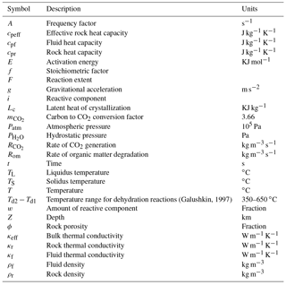
Table 1 contains the definitions of all the notations used in the paper. The effective rock heat capacity accounts for the latent heat of fusion in the crystallizing parts of the sill between the solidus (T_S) and liquidus (T_L) temperature of the magma (e.g., Galushkin, 1997):

$$\begin{array}{}\text{(3)}& {\displaystyle }\begin{array}{ll}{c}_{\mathrm{peff}}=c_{\mathrm{pm}}\left[\mathrm{1}+{\displaystyle \frac{L_c}{\left(T_{\mathrm{L}}-T_{\mathrm{S}}\right)c_{\mathrm{pm}}}}\right]& \text{if}\left[T_{\mathrm{S}}<T<T_{\mathrm{L}}\right]\\ c_{\mathrm{peff}}=c_{\mathrm{pr}}& \text{if}\left[T_{\mathrm{S}}>T\right]\end{array}.\end{array}$$

Sills are emplaced instantaneously at the specified time and temperature within the sedimentary column. The emplacement of multiple sills in the same step is possible. The time steps used for thermal diffusion after sill emplacement are automatically calculated based on the sill thickness and the characteristic time required for thermal diffusion. The time step is initially small in order to accurately resolve the thermal evolution of the contact aureole around the sill and is gradually increased once the energy released by the cooling sill is dissipated.

Dehydration reactions in the host rock are implemented by modifying the thermal diffusion equation when temperatures of the sediments increase within a certain range (Galushkin, 1997; Wang, 2012):

$$\begin{array}{}\text{(4)}& {\displaystyle }& {\displaystyle }\left[\mathit{\varphi }{\mathit{\rho }}_{\mathrm{f}}{c}_{\mathrm{pf}}+\left(\mathrm{1}-\mathit{\varphi }\right){\mathit{\rho }}_{\mathrm{r}}{c}_{\mathrm{peff}}\right]{\displaystyle \frac{\partial T}{\partial t}}=\mathrm{\nabla }\cdot \left(\mathit{\kappa }\mathrm{\nabla }T\right)-H\text{(5)}& {\displaystyle }& {\displaystyle }H={\displaystyle \frac{\left(\mathrm{1}-\mathit{\phi }\right){\mathit{\rho }}_{\mathrm{r}}{L}_{\text{d}}}{T_{\mathrm{d}\mathrm{1}}-T_{\mathrm{d}\mathrm{2}}}}{\displaystyle \frac{\partial T}{\partial t}}.\end{array}$$

3.3 Thermal maturation of organic matter

Vitrinite reflectance is a widely used indicator of thermal maturity and can be readily measured in the field. One of the most common methods used to calculate the thermal maturity of the source rock is the EASY%Ro method put forward by Sweeney and Burnham (1990). This model uses 20 parallel Arrhenius-type of first order reactions to describe the complex process of kerogen breakdown due to temperature increase. The reaction for the ith component is given by

$$\begin{array}{}\text{(6)}& {\displaystyle \frac{\text{d}{w}_i}{\text{d}t}}=-w_{i}A\exp \left[-{\displaystyle \frac{E_i}{R{T}^t}}\right],\end{array}$$

where w_i is the amount of material for component i, E_i is the activation energy for the given reaction and T^t is time-dependent temperature.

The total amount of material reacted is obtained by summing up the individual reactions:

$$\begin{array}{}\text{(7)}& {\displaystyle \frac{\text{d}w}{\text{d}t}}=\sum _i{\displaystyle \frac{\text{d}{w}_i}{\text{d}t}}.\end{array}$$

The fraction of reactant converted is

$$\begin{array}{}\text{(8)}& F=\mathrm{1}-{\displaystyle \frac{w}{w_{\mathrm{0}}}}=\mathrm{1}-\sum _i{f}_i\left({\displaystyle \frac{w_i}{w_{\mathrm{0}i}}}\right),\end{array}$$

from which the vitrinite reflectance can be readily calculated by

$$\begin{array}{}\text{(9)}& \mathit{\%}\text{Ro}=\exp \left(-\mathrm{1.6}+\mathrm{3.7}F\right).\end{array}$$

The amount of TOC that has reacted for any given time can be calculated by

$$\begin{array}{}\text{(10)}& \text{TOC}\left(t\right)={\text{TOC}}_{\text{o}}F\left(t\right),\end{array}$$

and the rate of organic matter degradation by

$$\begin{array}{}\text{(11)}& R_{\mathrm{om}}=\left(\mathrm{1}-\mathit{\varphi }\right){\mathit{\rho }}_{\mathrm{r}}{\displaystyle \frac{\partial \text{TOC}}{\partial t}}.\end{array}$$

The maximum amount of TOC that can be reacted by this method is 85 % of the initial total. Note that, in the inner part of the contact aureole close to the sill, data show that all of the organic matter has been reacted or removed (e.g., LA1/68 in Sect. 5.2.2). We assume that all of the hydrocarbons released during thermal degradation are converted into carbon dioxide. The amount of organic carbon dioxide generated ($R_{{\mathrm{CO}}_{\mathrm{2}}})$ for a time step is given by

$$\begin{array}{}\text{(12)}& R_{{\mathrm{CO}}_{\mathrm{2}}}=R_{\mathrm{om}}{m}_{{\mathrm{CO}}_{\mathrm{2}}},\end{array}$$

where $m_{{\mathrm{CO}}_{\mathrm{2}}}$ is a stoichiometric conversion factor (3.67) to transform carbon into carbon dioxide. Note that metamorphism of sedimentary rocks will generate CH₄ (e.g., Aarnes et al., 2010; Iyer et al., 2017a), but in our model the reacted carbon is recalculated to CO₂. If needed, the CO₂ model output can be easily converted to either C or CH₄.

The latent heat of organic maturation is accounted for in the energy equation:

$$\begin{array}{ll}{\displaystyle }& {\displaystyle }\left[\mathit{\varphi }{\mathit{\rho }}_{\mathrm{f}}{c}_{\mathrm{pf}}+\left(\mathrm{1}-\mathit{\varphi }\right){\mathit{\rho }}_{\mathrm{r}}{c}_{\mathrm{peff}}\right]{\displaystyle \frac{\partial T}{\partial t}}\\ {\displaystyle }& {\displaystyle }=\mathrm{\nabla }\cdot \left(\mathit{\kappa }\mathrm{\nabla }T\right)-H-L_{\mathrm{om}}{R}_{\mathrm{om}}.\end{array}$$

3.4 Mineral decarbonation

Carbonate minerals undergo decarbonation reactions as they are heated to high temperatures. This results in mineral transformations and the release of inorganic carbon dioxide which may significantly add to the CO₂ budget associated with igneous intrusions. The amount of inorganic CO₂ liberated during metamorphic transformation over a range of temperatures and fluid pressures for marl, dolomite and dolomite/evaporite mixture is pre-computed as a phase diagram using Perple_X (Connolly and Petrini, 2002) (Fig. 1). The model evaluates the total amount of inorganic CO₂ liberated by carbonate layers based on the temperature and pressure evolution of the layer through time within the phase diagrams. Fluid pressure within the sedimentary column is calculated by integrating the fluid density over depth in addition to atmospheric pressure:

$$\begin{array}{}\text{(13)}& P_{{\mathrm{H}}_{\mathrm{2}}\mathrm{O}}=P_{\text{atm}}+\underset{Z_{min}}{\overset{Z_{max}}{\int }}{\mathit{\rho }}_{\mathrm{f}}\mathit{g}.\end{array}$$

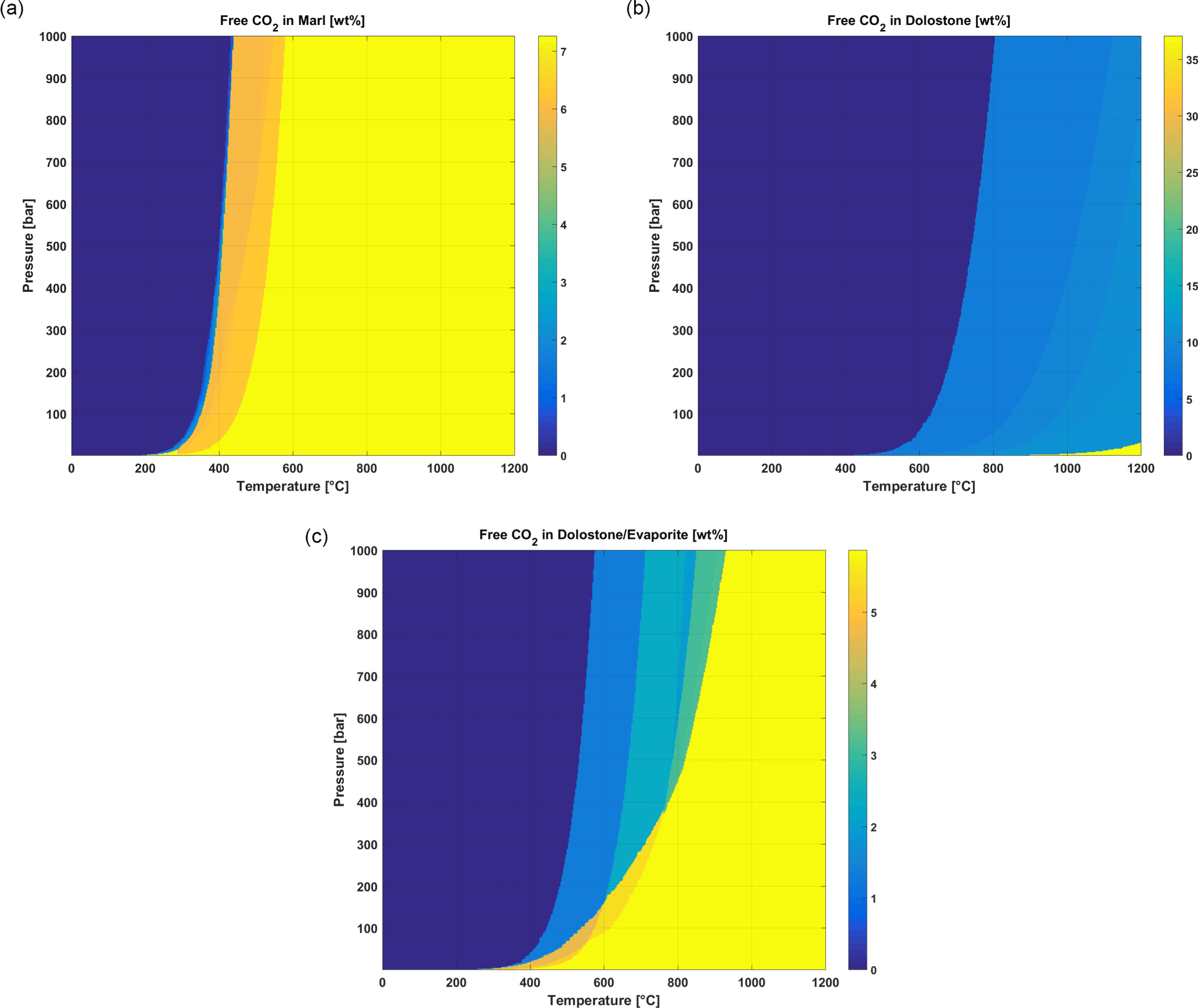
Figure 1 Phase diagrams generated by Perple_X showing the amounts of inorganic CO₂ liberated with respect to temperature and pressure for marl (a), dolostone (b) and dolostone/evaporite (c).

3.5 Model mesh and time stepping

The entire sedimentary column including the eroded layers and igneous intrusions is reconstructed and the column nodes and elements for the FEM model are generated using the user-specified resolution. The nodes are initially collapsed onto each other in depth. Each sedimentary node is assigned a time during which it is expanded (or deposited) within the sedimentary column based on the layer age and its thickness. All of the elements and nodes associated with each igneous intrusion are expanded simultaneously during the corresponding emplacement time. Eroded layers are removed in a single time step specified by the erosion age and the corresponding nodes are collapsed. In order to correctly capture thermal diffusion across the large thermal gradient adjacent to a hot intrusion, the time step is initially very small and exponentially increases during the heating period after sill emplacement and before the next depositional event. The heating period of the sill, over which the exponential time sub-stepping is used, is analytically determined from the characteristic diffusion time for the sill thickness (Jaeger, 1959).

Table 2 List of variables in the “rock” struct variable of the output file.

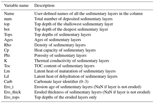
Table 3 List of variables in the “sill” struct variable of the output file.

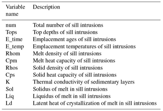
Table 4 List of variables in the “welldata” struct variable of the output file.

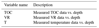
Table 5 List of variables in the “result” struct variable of the output file.

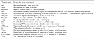
Table 6 List of variables in the “release” struct variable of the output file.

3.6 Model limitations

• The model is one-dimensional and will therefore not resolve thermal effects that would require a full 3-D model.

• The model does not account for advective transport of heat through the system by fluids. However, previous models have shown that this process would be dominant only in high permeability systems or at the sill edges/tips in low permeability systems (Iyer et al., 2013, 2017a). Therefore, the model presented in this paper works well for relatively low permeability systems with shales, mudstone, etc., and when the sedimentary column passes through the sill interior away from the edges. Nevertheless, in some cases the effects of hydrothermal activity may be visible where the thermal aureole is larger above than below the sill and is recorded by vitrinite reflectance data (Galushkin, 1997; Wang and Manga, 2015). In such cases, the user may use an enhanced thermal conductivity (up to 5 times the usual rock conductivity) in the layer above the sill following the Nusselt number approach to account for hydrothermal activity and match field data. Note that care should be taken to check if the same effect can also be attributed to changes in other material properties or geological processes.

• The model does not account for other mineral reactions in the contact aureole besides decarbonation of carbonates. The various mineral reactions possible in the contact aureole can be implemented as an add-on module to the model if needed using the thermal evolution of the sedimentary column obtained from the model. Similarly, correlation to other maturity parameters such as mineralogical markers or biomarkers (e.g., Muirhead et al., 2017) can be performed by the user using the time–temperature evolution from the model if so desired.

• The model assumes that TOC conversion in all types of sedimentary rocks can be estimated by using the EASY%Ro method with a maximum conversion value of 85 %. Although, this is a good first approximation, it cannot account for the complete loss of carbon in zones very close to the sill–host rock interface which would result in an underestimation of the released gases (Svensen et al., 2015). On the other hand, the provenance of the sedimentary rock can also significantly affect how kerogen present in organic matter reacts to form hydrocarbons, which may result in a reduction in the amount of convertible organic matter due to the presence of inert kerogen (Iyer et al., 2017a; Pepper and Corvi, 1995).

4 Model output

The model input and results are presented with the help of a graphical user interface (GUI) (Sect. 4.6). Model data are written out as a single .mat (Matlab data) file in the same directory as the user-defined path for the input Excel file and with the same filename. The file contains five “struct” variables of which three contain input information (rock, sill and welldata) and the other two contain model results (result and release). The structure of the variables is described below.

4.1 Struct variable: rock

This variable contains input information on the sedimentary layers in the column including the eroded layers. The information is saved as variables given in Table 2 and is sorted according to their top depths. Note that top depths are corrected for the eroded layers that are also included.

4.2 Struct variable: sill

This variable contains input information on sill intrusions in the column. The information is saved as variables given in Table 3 and is sorted according to their top depths.

4.3 Struct variable: welldata

This variable contains input information on measured TOC, VR and temperature data for the sedimentary column. The information is saved as variables given in Table 4.

4.4 Struct variable: result

This variable contains the model results which are saved for every time step when applicable; i.e., variables that change over time have rows corresponding to the element or node number (depending on where they are defined) and columns corresponding to the time step number. The information is saved as variables given in Table 5.

4.5 Struct variable: release

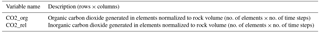
This variable contains the amounts of CO₂ released for every time step normalized to rock volume. The information is saved as variables given in Table 6.

4.6 Output graphical user interface

The GUI presented during and after the model run contains three tabs containing graphical representations of the input data, time evolution of model results and CO₂ release through time. An explanation of the tabs is given below using a hypothetical test case consisting of a sedimentary column with two sill intrusions and three eroded layers.

4.6.1 Input tab

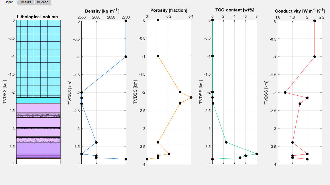
The leftmost subplot of the input tab contains the reconstructed sedimentary column where the layers are colored according to their depositional age (http://www.stratigraphy.org/index.php/ics-chart-timescale) (Fig. 2). The sedimentary column also contains eroded layers (hatched) and sill intrusions (speckled). The name and depositional age of a layer can be found by right-clicking the layer. The other subplots in the input tab contain information on the density, porosity, initial TOC content and thermal conductivity of the sedimentary layers. The values of these variables are plotted at the corresponding layer top depth.

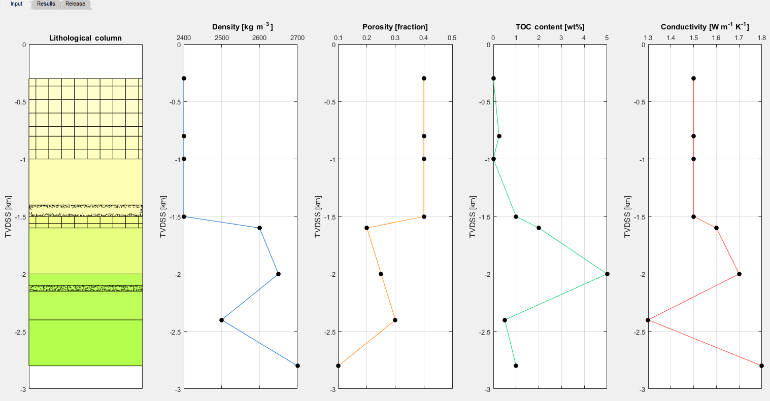
Figure 2 Snapshot of the input tab generated for a hypothetical sedimentary column with two sill intrusions and three eroded layers. Right-clicking a layer in the sedimentary column provides the name and depositional/erosional age of the layer.

4.6.2 Results tab

The results tab consists of the evolution of temperature, vitrinite reflectance, TOC content, maximum temperature, hydrostatic pressure, inorganic and organic CO₂ release within the sedimentary column over simulated time (Fig. 3). The evolution of these variables can be played or stepped through using the player controls in the top left corner. Alternatively, the user can jump directly to the desired geological time by inputting it in the player control. Note that this results in the plot jumping to the time step nearest the desired time input. Regions containing sill intrusions are highlighted in gray. Users can copy plot data at any time step by right-clicking the curve.

Figure 3 Snapshot of the results tab generated for a hypothetical sedimentary column with two sill intrusions and three eroded layers. Right-clicking any curve allows the user to copy curve data.

Figure 4 Snapshot of the release tab generated for a hypothetical sedimentary column with two sill intrusions and three eroded layers. Right-clicking any curve allows the user to copy curve data.

Figure 5 Input tab for the Utgard High example.

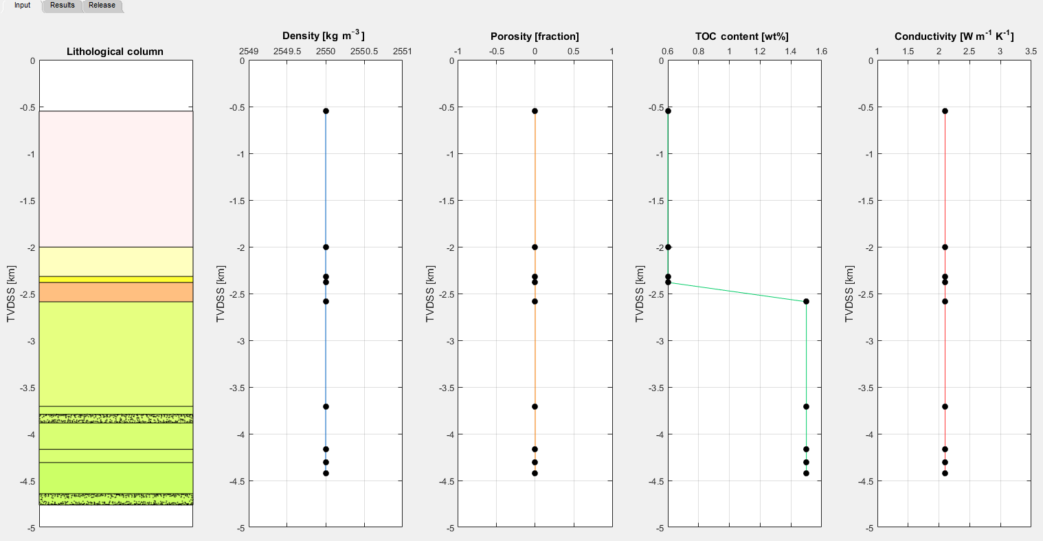
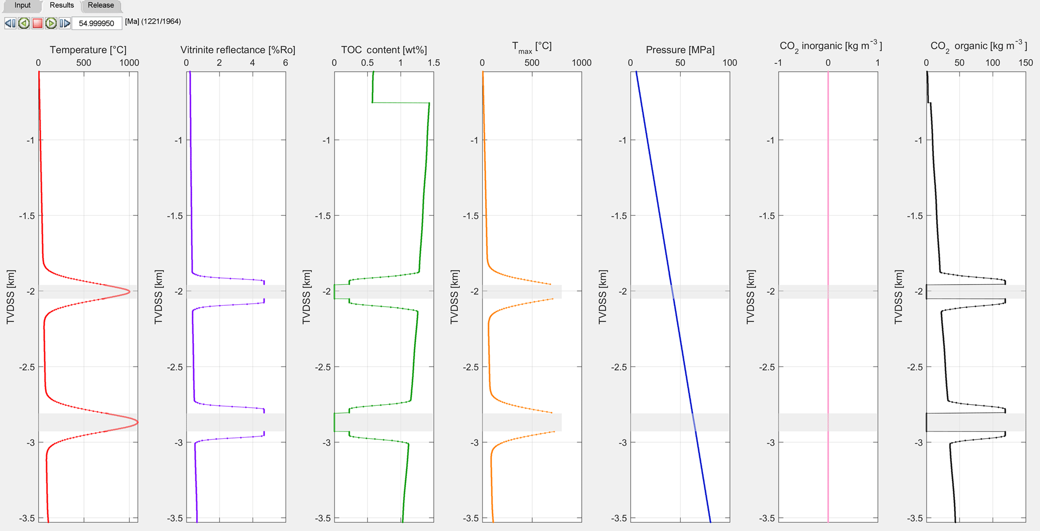
Figure 6 Results tab 50 years after the emplacement of sills at 55 Ma for the Utgard High example. Sediments around the sills are heated and CO₂ is liberated as organic matter is thermally degraded.

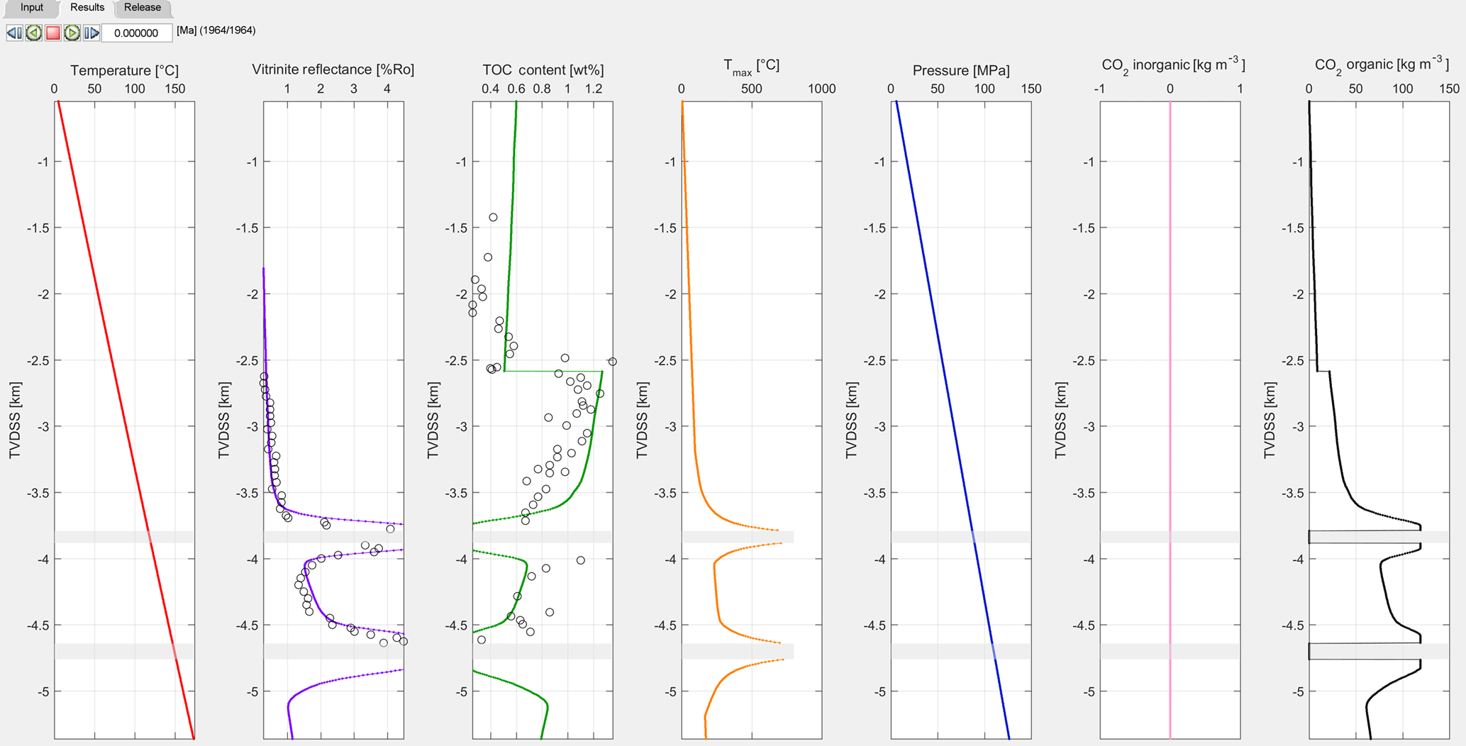
Figure 7 Results tab at the end of the simulation time for the Utgard High example. The present-day VR and TOC values (circles) show a good match with the model results.

4.6.3 Release tab

The release tab plots the cumulative amount and rates of release of organic and inorganic CO₂ due to heating of the sedimentary layer by sill intrusions (Fig. 4). The cumulative amount and release rates are summed over the entire sedimentary column. The user can use the cumulative amount of gas released to easily upscale to basin scales by multiplying the value by the area affected by sill intrusions. Users can copy plot data by right-clicking the curve.

5 Examples

The examples below are provided with the code and are used to benchmark observations to model results.

5.1 Utgard High

The Utgard sill complex is part of the North Atlantic Igneous Province (NAIP) in the Vøring and Møre Basins, off the shore of Norway. This region underwent massive volcanic activity at the Paleocene–Eocene boundary around ∼ 55 Ma (Aarnes et al., 2015). The Utgard High borehole 6607/5-2 was drilled through two sills emplaced in the Upper Cretaceous sedimentary layers. The drilled lithological column consists of nine layers with the oldest being deposited at 100 Ma (NPD Factpages, http://factpages.npd.no/factpages/) (Fig. 5). For simplicity, the material properties of the entire sedimentary column are set to constant values with the exception of TOC content. TOC content of the Paleocene and Upper Cretaceous sedimentary layers is set to initial values of 0.6 and 1.5 wt %, respectively. Carbonate and erosional layers are not considered. The modeled sedimentary layers are sequentially deposited at the sedimentation rate calculated from the layer top ages. The two sills are emplaced simultaneously within the Nise and Kvitnos formations at 55 Ma at a temperature of 1150 ^∘C. Sedimentary rocks around the emplaced sills are progressively heated as the sills cool. The vitrinite reflectance values increase and the TOC content is reduced by thermally degrading organic matter to form CO₂ (Fig. 6). Sedimentation after sill emplacement results in further burial and extension to produce the present-day sedimentary column. Vitrinite reflectance and TOC data from the Norwegian Petroleum Directorate (NPD) and a previous study (Aarnes et al., 2015) are used to benchmark the model and match very well with the modeled results (Fig. 7). Further information about the geological and model setting can be found in Aarnes et al. (2015) and the input file “1d_sill_input_utgard.xlsx”.

Figure 8 Input tab for KL1/78.

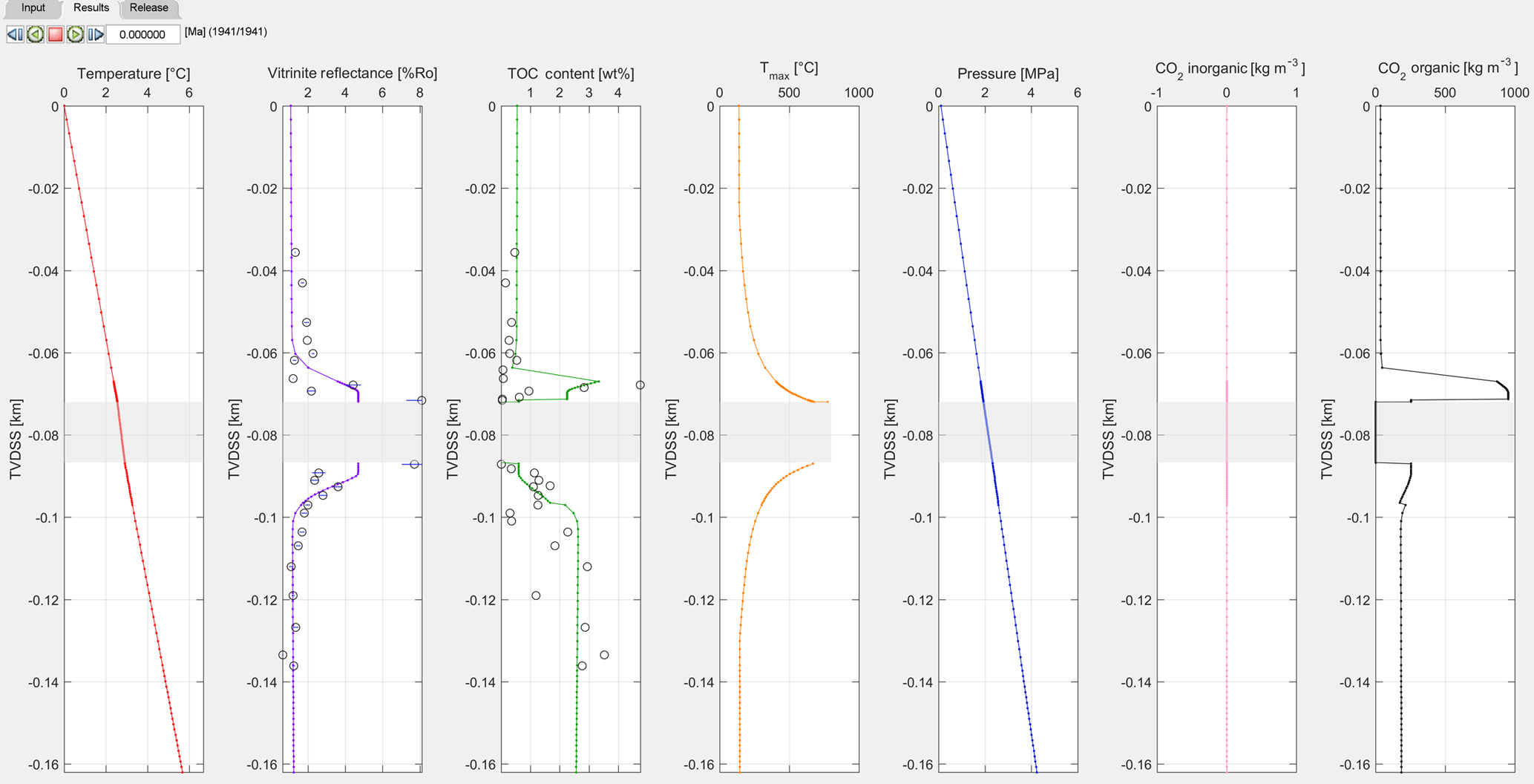
Figure 9 Results tab at the end of the simulation time for KL1/78 shows a good match to present-day TOC and VR values.

Figure 10 Input tab for LA1/68.

5.2 Karoo

The Karoo Large Igneous Province was emplaced through the Karoo Basin in South Africa in the Early Jurassic. The basin contains sills and dykes of varying thickness (Chevallier and Woodford, 1999; du Toit, 1920; Svensen et al., 2015; Walker and Poldervaart, 1949), emplaced at about 182.6 Ma (Svensen et al., 2012). The basin stratigraphy consists of the Upper Carboniferous to the Triassic Karoo Supergroup and is divided into five groups (the Dwyka, Ecca, Beaufort, Stormberg and Drakensberg groups) with a postulated maximum cumulative thickness of 12 km and a preserved maximum thickness of 5.5 km (Tankard et al., 2009). The depositional environments of the sediments range from marine and glacial (the Dwyka Group), marine to deltaic (the Ecca Group), to fluvial (the Beaufort Group) and finally eolian (the Stormberg Group) (Catuneanu et al., 1998). The Karoo Basin is overlain by 1.65 km of preserved volcanic rocks of the Drakensberg Group, consisting mainly of stacked basalt flows erupted in a continental and dry environment (e.g., Duncan et al., 1984). Several recent studies have been devoted to contact metamorphism of the organic-rich Ecca Group (Aarnes et al., 2011b; Moorcroft and Tonnelier, 2016) and the possible consequences of thermogenic methane venting on the Early Jurassic climate (Svensen et al., 2007, 2015). Here, we present two borehole cases from the central (borehole KL1/78) and eastern (borehole LA1/68) parts of the basin previously studied and modeled by Aarnes et al. (2011b) and Svensen et al. (2015), respectively. The details regarding the relative timing of sill emplacement are poorly constrained, and we thus use the same age for all sills. If the sills are closely spaced, this will result in a higher maximum temperature in the sedimentary rocks between the sills (see Aarnes et al., 2011b). For the erosion history of the Karoo Basin, we refer to Braun et al. (2014) and a rapid Late Cretaceous erosion event.

5.2.1 Karoo KL1/78

The first example from the Karoo Basin is a short borehole with a length of 136 m that penetrates the Tierberg, Whitehill and Prince Albert formations. However, these formations underlie a massive erosion sequence consisting of 2.5 km of extrusives (Drakensberg Group) and 1.5 km of sediments (Stormberg and Beaufort groups) and are also included in the model. The borehole penetrates a single 15 m thick sill at a depth of 72 m (Fig. 8). The sill is emplaced within the Prince Albert Formation at 182.6 Ma at a temperature of 1150 ^∘C. Initial average TOC data for the sedimentary layers away from the sill intrusion are not known but can be roughly estimated using present-day values; i.e., the TOC values will be higher than current values, as TOC is thermally broken down close to the intrusion. The initial input TOC data are subsequently refined so that a better match of the model results to the observed data is obtained, thereby highlighting how the model can be used to constrain initial conditions within the sedimentary column (Fig. 9). The importance of considering the entire basin history when constructing the model is also emphasized by the VR results. The values of the VR results unaffected by the sill would be much lower than the observed values if the eroded sequences are not considered. Addition of these layers to the model results in added burial than would be expected by just using the 136 m deep borehole. This translates the VR curve laterally, thereby better fitting the observed values (Fig. 9). The final model shows a good fit of TOC and VR to present-day values. Model input data can be found in “1d_sill_input_kl178.xlsx”.

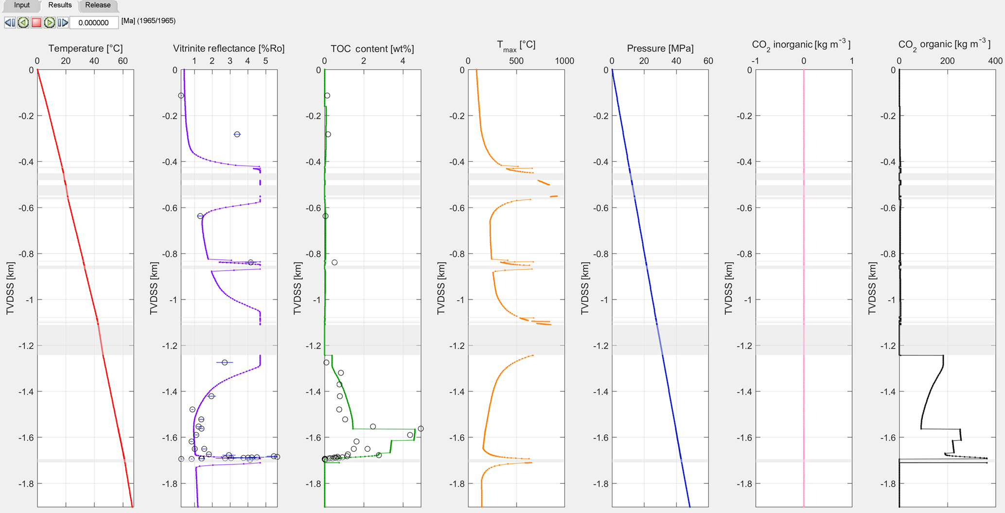
Figure 11 Results tab at the end of the simulation time for LA1/68 shows a good match to present-day TOC and VR values.

Figure 12 Input tab for the pluton example.

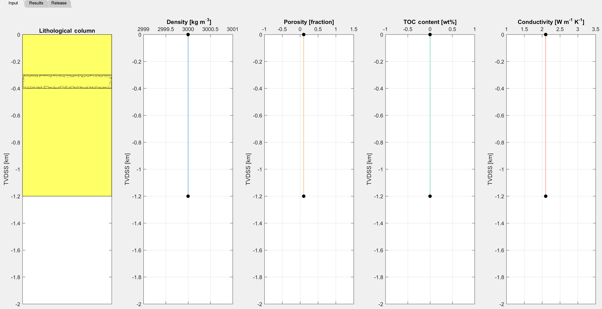
Figure 13 Results tab at the end of the simulation time for the pluton example. VR and TOC data are not present for this hypothetical case.

5.2.2 Karoo LA1/68

The second example from the Karoo Basin is a borehole with a length of 1711 m that penetrates the basin down to the basement (Svensen et al., 2015). An additional erosional sequence consisting mostly of the Drakensberg lavas and a minor section of the Stormberg Group is also added. The borehole penetrates multiple sills throughout the entire column with thicknesses ranging from 2 to 132 m (Fig. 10). Initial average TOC data for the sedimentary layers are estimated from present-day values. Similar to the previous example, material properties are iteratively changed within realistic bounds to arrive at an initial setup that matches the final observations well (Fig. 11). Model input data can be found in “1d_sill_input_la168.xlsx”.

5.3 Intrusion into a pluton

This example has been added to provide an instance where the user may be interested in modeling the thermal aureole of an emplaced sill or dyke but without the effects associated with deposition of sedimentary layers and the thermal evolution of a basin, e.g., emplacement within an igneous or metamorphic rock. Here, we consider an emplacement of a 100 m thick sill into a 1.2 km thick igneous body that has cooled to a uniform temperature of 30 ^∘C (Fig. 12). The host rock is constructed by defining top and bottom layers with the same material properties and ages that are very close to each other (the code does not allow for two layers with the exact same age). In this example, the top and bottom layers have ages of 10 and 10.0001 Ma, respectively, and the intrusion is emplaced at 1 Ma. A constant temperature for the host rock is defined by assigning the same temperature, 30 ^∘C, to both intervals in the temperature tab of the Excel input file. Thus, the thermal evolution of the intrusion can be investigated independent of burial effects of a sedimentary basin if so desired (Fig. 13). Further information about the model setting can be found in the input file “1d_sill_input_dyke.xlsx”.

6 Conclusions

SILLi is a numerical model that quantifies the thermal evolution of contact aureoles around sills emplaced in sedimentary basins. The model includes the basin history (burial and erosion), thus providing background-maturation levels of organic matter and consequently more realistic gas production estimates.

SILLi is a user-friendly tool that is written in Matlab and uses Excel for input data.

The 1-D tool allows for the quick quantification of the thermal effects of sill intrusions. The results can be therefore used to further constrain and test the initial conditions that may have been present within the lithological column that match present-day observations.

Model output includes peak temperature profiles, post-metamorphic TOC content, vitrinite reflectivity and the cumulative amount and rate of CO₂ generation. These values can be readily upscaled to basin scales if the sill extent is known. The amount of CO₂ can also be easily converted to other carbon-bearing gases such as CH₄.

Our three case studies demonstrate a good fit between aureole data (TOC and vitrinite reflectivity) and model output, showing that the model can be successfully applied to basins in various global settings.