Improvements to the hydrological processes of the Town Energy Balance model (TEB-Veg, SURFEX v7.3) for urban modelling and impact assessment

Climate change and demographic pressures are affecting both the urban water balance and microclimate, thus amplifying urban flooding and the urban heat island phenomena. These issues need to be addressed when engaging in urban planning activities. Local authorities and stakeholders have therefore opted for more nature-based adaptation strategies, which are especially suitable in influencing hydrological and energy processes. Assessing the multiple benefits of such strategies on the urban microclimate requires high-performance numerical tools. This paper presents recent developments dedicated to the water budget in the Town Energy Balance for vegetated surfaces (TEB-Veg) model (surface externalisée; SURFEX v7.3), thus providing a more complete representation of the hydrological processes taking place in the urban subsoil. This new hydrological module is called TEB-Hydro. Its inherent features include the introduction of subsoil beneath built surfaces, the horizontal rebalancing of intra-mesh soil moisture, soil water drainage via the sewer network and the limitation of deep drainage. A sensitivity analysis is then performed in order to identify the hydrological parameters required for model calibration. This new TEB-Hydro model is evaluated on two small residential catchments in Nantes (France), over two distinct periods, by comparing simulated sewer discharge with observed findings. In both cases, the model tends to overestimate total sewer discharge and performs better under wet weather conditions, with a Kling–Gupta efficiency (KGE) statistical criterion greater than 0.80 vs. approximately 0.60 under drier conditions. These results are encouraging since the same set of model parameters is identified for both catchments, irrespective of meteorological and local physical conditions. This approach offers opportunities to apply the TEB-Hydro model at the city scale alongside projections of climate and demographic changes.

1 Introduction

Cities consume space and energy, generate pollution and nuisances, and remain vulnerable to natural or manmade hazards, such as floods and urban heat islands (hereafter denoted UHIs). Climate change is likely to exacerbate all these phenomena (EEA, 2012). Adapting cities to global changes, including climate change and demographic pressures, has become a major challenge in the planning policy field. The reliance on nature-based solutions (hereafter denoted NBSs), e.g. green and blue infrastructure, has been approved as a part of sustainable urban development (sustainable urban drainage systems, water and pollution source control, building insulation) and is therefore recommended for future applications (Hamel et al., 2013; EC, 2015). However, evaluating such adaptation and mitigation strategies requires conducting impact studies capable of assessing the various amenities these solutions can offer, along with their corresponding interactions (energy, thermal comfort, water, landscaping, etc.) (Bach et al., 2014). With regards to hydro-microclimatic patterns, the integration of urban green spaces and vegetation promotes water infiltration as well as evapotranspiration (or latent heat flux). For modelling purposes, evapotranspiration is thus a key element since it affects both the urban water and energy budgets (Mitchell et al., 2008).

Despite increased interest in the field of urban hydrology over recent years (Fletcher et al., 2013; Hamel et al., 2013; Schirmer et al., 2013; Salvadore et al., 2015), the various water- and energy-related processes involved are still rarely addressed with the same level of detail. Thus, the coupling between them tends to be oversimplified. In the past, the emphasis on the urban water cycle was directed at designing urban drainage systems and at system operations under extreme events (flooding). Hydraulic models have thus been used to analyse rainfall–runoff patterns during rainfall events, when evapotranspiration is not a major concern (Berthier et al., 2006; Fletcher et al., 2013). In recent decades, however, a more decentralised urban water management system has necessitated impact studies that focus on the urban water cycle as a whole. Consequently, urban hydrological models are being more heavily promoted, as opposed to hydraulic models. Yet these hydrological models still make use of a simple energy balance. Evapotranspiration is often calculated from a reference value of potential evapotranspiration, which takes into account soil moisture conditions and, in some instances, vegetation (DHI, 2001; Rodriguez et al., 2008; Rossman, 2010). At the local level, atmospheric demand is typically excluded as a limiting factor for evapotranspiration. In their state-of-the-art paper, Fletcher et al. (2013) noted that evapotranspiration in urban areas remains rather poorly explored.

Unlike hydrological models, urban microclimate models (Masson, 2000; Musy et al., 2015; Gros et al., 2016) provide a detailed solution to the energy and radiative budgets. Nonetheless, the water balance is often simplified in microclimate models, which can then lead to an alteration of the modelled latent heat fluxes (Grimmond et al., 2011). Malys et al. (2016) applied such a model with “SOLENE-microclimat” to evaluate the mitigation effects of vegetation on UHI. In the present model, however, soil moisture is not considered as a limiting factor, thus potentially leading to an overestimation of the cooling abilities of plants, especially under hot climate conditions. For example, the Town Energy Balance (TEB) scheme described by Masson (2000) is a mesoscale surface scheme dedicated to the urban environment. The urban environment is presented in a simplified manner by means of the street canyon approach (Oke, 1987). This approach averages the characteristics of urban covers and morphology (building height, construction materials, canyon aspect ratio, street orientation) inside a single grid mesh. It initially resolves detailed energy and radiative budgets of built-up areas (buildings and roads). Yet the hydrological part is more simply represented; i.e. (i) artificial surfaces (buildings and roads) are completely impervious, and (ii) water exchange is thus only taken into account between the surface and the atmosphere. Lemonsu et al. (2007) introduced both the rainfall interception capacities of built-up surfaces and integrated water infiltration through artificial surfaces, like roads, pavements and parking lots, into TEB in order to implement more realistic hydrological processes. The TEB model has evolved into TEB-Veg by integrating vegetated surfaces inside the street canyon. This step was made possible by use of the ISBA-DF model (interaction soil–biosphere–atmosphere – explicit vertical diffusion) (Boone et al., 2000) as part of the urban fabric (Lemonsu et al., 2012a). Interactions within the radiative, energy and water balances between natural and artificial surfaces are now taken into consideration. Nevertheless, while a detailed water balance for the subsoil of natural surfaces is indeed being calculated, the water processes occurring in the subsoil of artificial surfaces and their interactions with the surface are still being neglected.

The objective of this study is to develop a complete urban hydro-microclimate model, hereafter called TEB-Hydro, by integrating the subsoil under built-up surfaces and hydrological soil–surface interactions into the existing TEB-Veg model. This step will allow treating the energy and water budgets with the same level of detail, which is critical to the impact assessment of NBSs on a citywide scale. In the first step presented herein, the model concept will be described. Attention will be placed on the model's hydrological component and recent model developments, since the energy and radiation components of the model have not changed, performed by Masson (2000) and Lemonsu et al. (2012a). The experimental sites and observational data will then be presented. Afterwards, the model evaluation will be provided in Sect. 4 by means of analysing the simulations run by the new model version.

2 Description of the TEB-Hydro hydrological model

TEB-Hydro is an evolved version of TEB-Veg, using surface externalisée (SURFEX) v7.3 (Lemonsu et al., 2012a). It was developed on the SURFEX modelling platform (Masson et al., 2013) and can be applied at the city scale as well as the catchment scale. Like TEB-Veg, TEB-Hydro is based on a regular grid mesh with a resolution varying between several hundred and several decametres. This model can be run either coupled with other meteorological models or in offline mode forced by observed atmospheric data. It combines two surface schemes, TEB (Masson, 2000) and ISBA-DF (Boone et al., 2000), both of which rely on an integrated tiling approach and describe energy and water exchange between the urban and natural subsoils, the surface and atmosphere, respectively. The urban environment is represented by three compartments, namely buildings (roofs and walls), roads (streets, pavements and parking lots) and gardens. This section will present new model developments based on the existing TEB-Veg model version. A general description of the hydrological processes will be laid out first, followed by a discussion of the new developments dedicated to hydrological processes in urban subsoil (Fig. 1).

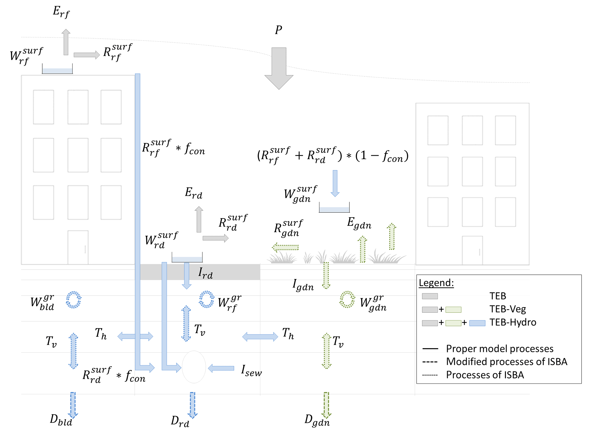
Figure 1 Diagram of the hydrological processes involved in the TEB-Hydro model; subscripts rf and bld stand for building compartment, rd for road compartment and gdn for garden compartment.

2.1 General principles of hydrological processes

Interactions between the energy balance (Eq. 1) and water balance (Eq. 2) are established via an explicit resolution of the evapotranspiration term (Eq. 3):

$$\begin{array}{}\text{(1)}& {\displaystyle }& {\displaystyle }{Q}^{*}+Q_{\mathrm{F}}=Q_{\mathrm{H}}+Q_{\mathrm{E}}+\mathrm{\Delta }{Q}_{\mathrm{S}}+\mathrm{\Delta }{Q}_{\mathrm{A}}\left[\mathrm{W}{\mathrm{m}}^{-\mathrm{2}}\right]\text{(2)}& {\displaystyle }& {\displaystyle }P+I=E+R+D+\mathrm{\Delta }W\left[\mathrm{kg}{\mathrm{m}}^{-\mathrm{2}}{\mathrm{s}}^{-\mathrm{1}}\right]\text{(3)}& {\displaystyle }& {\displaystyle }{Q}_E=E\cdot L_v\left[\mathrm{W}{\mathrm{m}}^{-\mathrm{2}}\right]\end{array}$$

where Q^∗ is the net all-wave radiation, Q_F the anthropogenic heat flux, Q_H the sensible heat flux, Q_E the latent heat flux, ΔQ_S the heat flux storage, ΔQ_A the net advection heat flux, P the total precipitation, I the water generated from anthropogenic activities (irrigation), E the evapotranspiration, R the total runoff, D the deep drainage, ΔW the variation in water storage both on the surface and in the ground during the simulation period and lastly L_v the latent heat of vaporisation (J kg⁻¹).

2.1.1 Evapotranspiration

Evaporation is calculated for each surface type E_∗ (kg m⁻² s⁻¹) (Fig. 1). For built-up surfaces, this value depends on both the surface specific humidity at saturation and the air humidity (inside the canyon for roads and above the canopy level for roofs) (Masson, 2000). Limitations are set by the maximum surface retention capacity of roofs ($W_{\max ,\mathrm{rf}}^{\mathrm{surf}}$, mm) and roads ($W_{\max ,\mathrm{rd}}^{\mathrm{surf}}$, mm), as represented by the surface water reservoirs. For natural surfaces, the various contributions from vegetation and natural subsoil are considered (Eq. 4) (Lemonsu et al., 2012a):

$$\begin{array}{}\text{(4)}& E_{\mathrm{gdn}}=E_{\mathrm{veg}}+E_{\mathrm{gr}}+E_{\mathrm{gr},i}+E_{\mathrm{s}},\end{array}$$

where E_veg is the vegetation evapotranspiration, E_gr,i and E_gr the evaporation from bare soil, respectively, with and without freezing and E_s the sublimation from snow. These terms are detailed in the SURFEX scientific documentation (see https://www.umr-cnrm.fr/surfex/IMG/pdf/surfex_scidoc_v2-2.pdf, last access: 4 September 2018).

2.1.2 Water interception

Water content changes in the interception water reservoirs of each surface type (denoted $W_{\ast }^{\text{surf}}$ in millimetres) are affected by precipitation and evapotranspiration rates, as indicated in Masson (2000) and Lemonsu et al. (2012a):

$$\begin{array}{}\text{(5)}& {\displaystyle \frac{\partial W_{\ast }^{\mathrm{surf}}}{\partial t}}=P-E_{\ast },\end{array}$$

where * stands for rooftops, vegetation or bare ground surfaces.

For the road interception reservoir, the original evolution equation has been modified by including a slight water infiltration rate (I_rd) (in mm s⁻¹), since roads are never totally impervious (Ramier et al., 2011):

$$\begin{array}{}\text{(6)}& {\displaystyle \frac{\partial W_{\mathrm{rd}}^{\mathrm{surf}}}{\partial t}}=P-E_{\mathrm{rd}}-I_{\mathrm{rd}}.\end{array}$$

I_rd is defined as a constant value over which the model must be calibrated. Typical values for this parameter can be found in Ramier et al. (2011).

2.1.3 Surface runoff

According to Masson (2000), when $W_{\ast }^{\mathrm{surf}}$ (mm) exceeds the maximum reservoir capacity ($W_{max,\ast }^{\mathrm{surf}}$), surface runoff is produced ($R_{\ast }^{\mathrm{surf}}$, in mm s⁻¹). From this point forward, it is collected by the stormwater sewer network, depending on the effective connected impervious area fraction (f_con) (Sutherland, 2000). The surface runoff not collected by the stormwater sewer network $\left(\right(R_{\mathrm{rf}}^{\mathrm{surf}}+R_{\mathrm{rd}}^{\mathrm{surf}})\cdot (\mathrm{1}-f_{\mathrm{con}}\left)\right)$ is then added to the throughfall over natural surfaces, where it can infiltrate into the subsoil with maximum infiltration capacity, according to the Green–Ampt approach (Abramopoulos et al., 1988; Entekhabi and Eagleson, 1989; Lemonsu et al., 2012a).

The urban runoff R_town (mm s⁻¹) used to determine total stormwater sewer discharge ($Q_{\mathrm{town}}^{\mathrm{tot}}$) is composed of several sources, namely

$$\begin{array}{}\text{(7)}& R_{\mathrm{town}}=R_{\mathrm{rf}}^{\mathrm{surf}}\cdot f_{\mathrm{con}}+R_{\mathrm{rd}}^{\mathrm{surf}}\cdot f_{\mathrm{con}}+R_{\mathrm{sew}}+R_{\ast }^{\mathrm{subsurf}},\end{array}$$

where $R_{\mathrm{rf}}^{\mathrm{surf}}\cdot f_{\mathrm{con}}$ and $R_{\mathrm{rd}}^{\mathrm{surf}}\cdot f_{\mathrm{con}}$ are, respectively, the roof and road surface runoff connected to the sewer network (in mm s⁻¹); R_sew is the runoff in the sewer network due to soil water infiltration (mm s⁻¹) and $R_{\ast }^{\mathrm{subsurf}}$ the subsurface runoff from each compartment (mm s⁻¹), as calculated in Eq. (16).

2.1.4 Vertical water transfer

Surface water infiltration, as described above, constitutes an input to the subsoil of both the garden and road compartments. The water is then transferred vertically from layer to layer, accounting for the liquid water transfer and water vapour transfer referenced in Boone et al. (2000). This process depends solely on pressure gradients and enables taking different hydraulic soil properties into consideration. At the bottom of each soil column, the vertical water transfer is adapted by taking boundary conditions into account. The resulting outgoing water flux of the model is called deep drainage D_∗, with this parameter being slightly modified for TEB-Hydro (Sect. 2.2.3).

2.2 Inclusion of hydrological processes in the urban subsoil

In accordance with the soil description of urban gardens provided in Lemonsu et al. (2012a), soil compartments are now considered within the category of built-up surfaces, i.e. roads and buildings (Fig. 1). All three soil columns are represented by horizontal layers with an identical vertical grid, in order to compute subsurface soil water transport. The thickness of each layer increases downward, with a finer grid resolution on top. In the case of the road compartment, the upper soil layers are represented by structural layers, in accordance with Bouilloud et al. (2009). By integrating natural soil below urban surfaces, the hydrological processes in the soil (vertical water transfer and deep drainage) of both road and building compartments are being adapted from the garden compartment. Water infiltration through the road structure is thus now considered as a recharge of soil moisture in the road compartment soil column. No water however is input into the building compartment soil column.

2.2.1 Horizontal water transfer

The lateral water interactions of each soil layer, from the three distinct compartments of the same grid cell, are taken into account (Fig. 1). In considering the structural layers of the road compartment, the horizontal transfer in the upper soil layers is computed solely between the garden and building compartments. Below that level, all three compartments are taken into account. This approach is based on the principle of an exponential decay in the water content, tending towards the mean soil moisture of all three compartments, which is limited by soil moisture content at the wilting point. The soil texture is assumed to be homogeneous for all three compartments within a given grid cell. Moreover, no lateral transfer is taking place between the grid cells of the model. The lateral intra-mesh soil moisture transfer for each soil layer is described as follows:

$$\begin{array}{}\text{(8)}& {\displaystyle \frac{\partial W_{\ast }^{\mathrm{gr}}}{\partial t}}=-{\displaystyle \frac{\mathrm{1}}{\mathit{\tau }}}\cdot {\displaystyle \frac{\stackrel{\mathrm{‾}}{K_{\mathrm{sat}}}}{K_i}}.\end{array}$$

Updating the soil moisture content in each layer and compartment after each time step yields

$$\begin{array}{}\text{(9)}& W_{\ast }^{\mathrm{gr}{,}^{\prime }}=\stackrel{\mathrm{‾}}{W^{\mathrm{gr}}}+\left(W_{\ast }^{\mathrm{gr}}-\stackrel{\mathrm{‾}}{W^{\mathrm{gr}}}\right)\cdot \exp \left(-\left({\displaystyle \frac{\mathrm{1}}{\mathit{\tau }}}\cdot {\displaystyle \frac{\stackrel{\mathrm{‾}}{K_{\mathrm{sat}}}}{K_i}}\right)\cdot \mathrm{d}t\right),\end{array}$$

with

$$\begin{array}{}\text{(10)}& {\displaystyle }\stackrel{\mathrm{‾}}{W^{\mathrm{gr}}}={\displaystyle \frac{\sum W_{\ast }^{\mathrm{gr}}\cdot f_{\ast }}{\sum f_{\ast }}},\end{array}$$

where $W_{\ast }^{\mathrm{gr}}$ and $W_{\ast }^{\mathrm{gr}{,}^{\prime }}$ are the soil moisture content for each compartment, respectively, before and after horizontal balancing (m³ m⁻³), $\stackrel{\mathrm{‾}}{W^{\mathrm{gr}}}$ is the mean soil moisture content of all compartments before balancing (m³ m⁻³), τ the time constant for 1 day, $\frac{\stackrel{\mathrm{‾}}{K_{\mathrm{sat}}}}{K_i}$ the ratio of the mean hydraulic conductivity at saturation of all three compartments to the hydraulic conductivity of each compartment, dt the numerical time step of the model(s) and f_∗ the fraction of each compartment.

2.2.2 Drainage of soil water via the sewer network

Various experiments and observations (Belhadj et al., 1995; Lerner, 2002; Berthier et al., 2004; Le Delliou et al., 2009) have shown that soil water drainage occurs when artificial networks are exposed to saturated soil moisture conditions. The ISBA soil pattern however is intended to depict the unsaturated zone rather than the saturated one. This pattern is based on a representation of the soil moisture state in agronomic terms (i.e. water content at wilting point, field capacity and saturation). When applying this approach, the infiltration rate into the sewer network (I_sew in m s⁻¹) is described in such a way that the hydraulic conductivity of the network soil layer (k_sew(W_gr) (m s⁻¹)) serves as the limiting factor, with a maximum value at saturation:

$$\begin{array}{}\text{(11)}& I_{\mathrm{sew}}=k_{\mathrm{sew}}\left(W_{\mathrm{gr}}\right)\cdot I_{\mathrm{p}}\cdot D_{\mathrm{sew}},\end{array}$$

where I_p is a parameter without any physical significance, indicating the sewer pipe water tightness (–), which must be calibrated; and D_sew is the sewer density within a single grid cell (–), as expressed by the ratio of the total sewer length in one grid cell (m) to the maximum total sewer length in a single grid cell of the entire study site (m). Let us note that this formulation has been adapted to TEB-Hydro from Rodriguez et al. (2008).

2.2.3 Deep drainage

In cities, artificial networks may play the role of rivers and thus contribute to draining soil water by means of infiltration. It has therefore been envisaged to limit deep drainage in order to favour soil water infiltration into the sewer networks during wet periods. For this purpose, the soil moisture emerging from the last layer of the model is partially or totally retained, according to a coefficient of recharge C_rech, until complete layer saturation. At each time step, the soil moisture content in the last layer n is thus updated according to

$$\begin{array}{}\text{(12)}& W_{\ast }^{\mathrm{gr},n}=W_{\ast }^{\mathrm{gr},n}+W_{\ast }^{\mathrm{gr},\mathrm{flux},n}\cdot C_{\mathrm{rech}}.\end{array}$$

Moreover, the deep drainage becomes

$$\begin{array}{}\text{(13)}& {\displaystyle }{D}_{\ast }=W_{\ast }^{\mathrm{gr},\mathrm{flux},n}\cdot \left(\mathrm{1}-C_{\mathrm{rech}}\right)\cdot d_n\cdot \mathit{\rho }/\mathrm{d}t,\end{array}$$

where $W_{\ast }^{\mathrm{gr},n}$ is the soil moisture content of the last layer n (m³ m⁻³), $W_{\ast }^{\mathrm{gr},\mathrm{flux},n}$ the soil moisture content derived from the outgoing water flux (m³ m⁻³), C_rech the coefficient of recharge (–) used to limit deep drainage, D_∗ the deep drainage (mm s⁻¹), d_n the thickness of the last layer, ρ the water density (kg m⁻³) and dt the numerical time step of the model(s).

If the deep layer is saturated, the excess moisture rises from layer to layer, with

$$\begin{array}{ll}{\displaystyle }& {\displaystyle }\text{the soil moisture content in upper layer}i-\mathrm{1},\\ \text{(14)}& {\displaystyle }& {\displaystyle }{W}_{\ast }^{\mathrm{gr},i-\mathrm{1}{,}^{\prime }}=W_{\ast }^{\mathrm{gr},i-\mathrm{1}}+max\left(\mathrm{0},W_{\ast }^{\mathrm{gr},i}-W_{\ast ,\mathrm{sat}}^{\mathrm{gr},i}\right)\cdot {\displaystyle \frac{d_{i-\mathrm{1}}}{d_i}}{\displaystyle }& {\displaystyle }\text{and the soil moisture content remaining in layer}i,\\ \text{(15)}& {\displaystyle }& {\displaystyle }{W}_{\ast }^{\mathrm{gr},i{,}^{\prime }}=min(W_{\ast }^{\mathrm{gr},i},W_{\ast ,\mathrm{sat}}^{\mathrm{gr},i}).\end{array}$$

If saturation was to reach the surface layer, then the excess moisture would be added to subsurface runoff, i.e.

$$\begin{array}{}\text{(16)}& R_{\ast }^{\mathrm{subsurf}{,}^{\prime }}=R_{\ast }^{\mathrm{subsurf}}+max\left(\mathrm{0},W_{\ast }^{\mathrm{gr},\mathrm{1}}-W_{\ast ,\mathrm{sat}}^{\mathrm{gr},\mathrm{1}}\right)\cdot {\displaystyle \frac{d_{\mathrm{1}}}{\mathrm{d}t}}\cdot \mathit{\rho },\end{array}$$

where $W_{\ast ,\mathrm{sat}}^{\mathrm{gr},i}$ is the soil moisture content at saturation (m³ m⁻³), $W_{\ast }^{\mathrm{gr},i{,}^{\prime }}$ and $W_{\ast }^{\mathrm{gr},i}$ the soil moisture content in current layer i, respectively, after and before update (m³ m⁻³), $W_{\ast }^{\mathrm{gr},i-\mathrm{1}{,}^{\prime }}$ and $W_{\ast }^{\mathrm{gr},i-\mathrm{1}}$ the soil moisture content in the upper soil layer i−1, respectively, after and before update (m³ m⁻³), $\frac{d_{i-\mathrm{1}}}{d_i}$ (–) the layer thickness ratio between upper layer i−1 and lower layer i, and $R_{\ast }^{\mathrm{subsurf}{,}^{\prime }}$ and $R_{\ast }^{\mathrm{subsurf}}$ the subsurface runoff, respectively, after and before update (mm s⁻¹).

2.3 TEB-Hydro output variables

In addition to the simulated hydrological output variables calculated in TEB-Veg (latent heat fluxes on all surfaces, soil moisture in each soil layer ($W_{\mathrm{gdn}}^{\mathrm{gr},i}$) and deep drainage (D_gdn) of the garden compartment), the TEB-Hydro model simulates soil moisture in each soil layer ($W_{\ast }^{\mathrm{gr},i}$) and the deep drainage (D_∗) under artificial surfaces. Other new model output variables include urban runoff (R_town) in the stormwater sewer network, with its components stemming from rooftops ($R_{\mathrm{rf}}^{\mathrm{surf}}\ast f_{\mathrm{con}}$) and road surfaces ($R_{\mathrm{rd}}^{\mathrm{surf}}\cdot f_{\mathrm{con}}$), soil water infiltration (R_sew) and the subsurface runoff from each compartment ($R_{\ast }^{\mathrm{subsurf}}$).

3 Experimental study areas and observational data

The experimental data are derived from two small urban catchments in the city of Nantes (France). The properties of these catchments, along with local observational data and the meteorological forcing data of the model, will be described below.

3.1 Experimental data

3.1.1 Rezé catchment

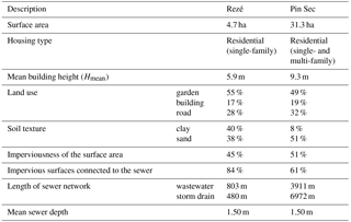
The Rezé experimental site is located in the southern part of the city of Nantes, close to the Atlantic coast (Fig. 2). This site was instrumented (for measurements of precipitation, rainwater network discharge and soil water) from 1993 to 1998, and a complete continuous database is available for that period. The climate is oceanic with an average annual rainfall of approximately 830 mm over this period; the year 1994 was the wettest. The 4.7 ha basin is entirely residential, comprising single-family homes with private gardens. The separate sewer network is divided into wastewater and stormwater sewers, with lengths of 803 and 480 m, respectively. The impervious surface area of the catchment accounts for 45 % of its total area, of which 84 % is connected to the stormwater system. A detailed site description can be found in Berthier et al. (1999) and Dupont et al. (2006) (Table 1). The Rezé catchment and its database have been the subject of several studies (Rodriguez et al., 2003; Berthier et al., 2004; Dupont et al., 2006; Lemonsu et al., 2007; Rodriguez et al., 2008). Berthier (1999) modelled the role of soil in generating urban runoff on the Rezé catchment. He studied both the hydrological aspects and site observations. Among other achievements, he examined the discharge observed in the wastewater sewer during the winter periods between 1993 and 1997, before estimating the discharge due to soil water infiltration; this value was then compared to the simulated base flow in the sewer network.

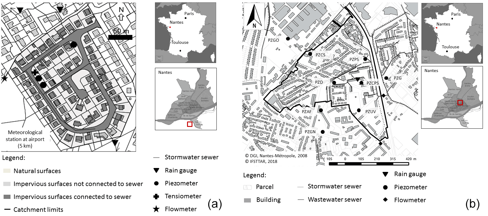
Figure 2 (a) The Rezé experimental site (from Dupont, 2001); (b) the Pin Sec experimental site. Maps to the right of the catchments indicate the location of Nantes (France) above and the Rezé and Pin Sec catchment locations (red square) in Nantes (middle).

Table 1 Summary of basin characteristics for both the Rezé and Pin Sec catchments.

3.1.2 Pin Sec catchment

The Pin Sec experimental site is located in the eastern section of Nantes; it has been a part of the Nantes Observatory for Urban Environments (ONEVU) since 2006 and contains a dense network of continuous measurement equipment (rain gauges, flow meters in the sewer networks, piezometers, tensiometers and microclimatological masts). To correspond with the simulation period of this study, rainfall patterns were analysed between May 2010 and September 2012, with an annual rainfall of approximately 700 mm recorded for the year 2011. The catchment area spans 31 ha and comprises some 2500 inhabitants (Le Delliou et al., 2009). The northern part of the site is characterised by single-family housing with private gardens, as opposed to the southern part, which encompasses four-storey multi-family buildings and public parks (Fig. 2b). The sewer network is separate, i.e. divided into wastewater and stormwater, with respective lengths of 6973 and 3911 m. Overall, 51 % of the total area is impervious, of which only 61 % was found to be connected to the stormwater sewer (according to a survey conducted by the Nantes metropolitan government). A summary description of this catchment is displayed in Table 1.

3.2 Meteorological forcing

Forcing the model with observations requires atmospheric data, such as precipitation, temperature, specific humidity, atmospheric pressure, wind speed and direction, and incoming shortwave and longwave radiation. For both experimental sites, the precipitation rates (with no snowfall for all simulation periods) were collected on-site by means of rain gauges. All other forcing data were generated from records at the nearby Météo-France weather station (Nantes Airport), including incoming solar radiation, cloudiness, pressure, air temperature and humidity at 2 m above ground and wind speed at 10 m above ground. To avoid the direct influence of the urban canopy, the forcing level height for temperature, humidity and wind speed had to be set above the roughness sublayer top; hence, the atmospheric data had to be adjusted accordingly (Lemonsu et al., 2012b).

4 Evaluation of the TEB-Hydro model

The TEB-Hydro model was evaluated by comparing the simulation output with both the observed total stormwater sewer discharge and the portion of this discharge due to soil water infiltration. Observations were derived from both experimental sites described above. Let us note that the local properties of these sites, as well as the simulation period, do vary. A sensitivity analysis performed on the Rezé catchment will be presented first. The hydrological parameters taken into account consist of the maximum retention capacity of the artificial surfaces $W_{max,\ast }^{\mathrm{surf}}$ (roads and buildings), a parameter describing the water tightness of the sewer pipe I_p, the maximum infiltration rate through the road structure I_rd, the fraction of impervious surface areas connected to the sewer network f_con and the deep drainage D_∗ (Sect. 2 and Table 2). In addition, the possible combined effects of these studied parameters will be analysed. As is typical for hydrological models, TEB-Hydro is calibrated on parameters that reveal the greatest model sensitivity. The model will then be evaluated on the observed total stormwater sewer discharge of both the Rezé and Pin Sec catchments. Simulations will be run using the TEB-Hydro model and compared to observations for the purpose of discussing the performance of recent model developments.

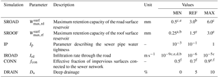
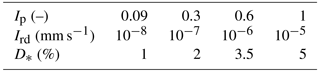
Table 2 Description of the hydrological parameters of the TEB-Hydro model as well as its MIN, MAX and REF values for the sensitivity analysis. The deep drainage values correspond to a coefficient of recharge of, respectively, 1.0, 0.95 and 0.90. The values for $W_{\max ,\mathrm{rd}}^{\mathrm{surf}}$, $W_{\max ,\mathrm{rf}}^{\mathrm{surf}}$, I_rd and f_con have been identified from either a literature review or in situ measurements (^a Hollis and Ovenden, 1988; ^b Berthier et al., 2004; ^c Lemonsu et al., 2007; ^d Ramier et al., 2011; ^e Furusho et al., 2013; ^f Allard, 2015).

4.1 Model configuration

The TEB-Hydro model (SURFEX v7.3) has been applied to a single grid point (1-D) at both experimental sites; it operates in offline mode and is forced by meteorological observations (Sect. 3.2) with a 1 h time step. The model's numerical time step equals 5 min. For both catchments, 12 soil layers were taken into account, and the road structure was divided into five artificial layers. Given the mean sewer system depth (1.50 m), the sewer pipe has been situated in the 10th soil layer. Natural surfaces are represented by bare ground, and low- and high-growth vegetation.

In the case of the Rezé catchment, the model was run over a 6-year period, from January 1993 to December 1998. The hydrological year begins in September, since the lowest base flow can be detected in August for the Nantes region. Its morphological data, radiative and thermal properties of materials (TEB), and soil and vegetation properties (ISBA) have all been taken into consideration, like in Lemonsu et al. (2007).

The simulation period for the Pin Sec catchment is 2.5 years, i.e. between May 2010 and September 2012. The morphological site data, radiative and thermal properties of materials (TEB), and soil and vegetation properties (ISBA) were determined on the basis of several sources (FluxSAP database, Furusho, 2012; Nantes metropolitan urban databank and Ecoclimap I, Faroux et al., 2013). Due to inconsistencies between previous studies (Le Delliou et al., 2009; Seveno et al., 2014), the Pin Sec catchment area has been delimited again using a Geographic Information System (GIS) (Fig. 2b).

4.2 Sensitivity analysis

A sensitivity analysis was conducted on the Rezé catchment; its aim was to better understand the role of each individual parameter in the various hydrological processes and to identify the processes responsible for greater model sensitivity and thus needing to be calibrated. Two types of analyses are generally encountered: local and global (Saltelli et al., 2004; Tang et al., 2007). For this study, a local analysis based on the one factor at a time (OFAT) method was chosen (Montgomery, 2017). This approach measures the influence of a parameter by the amplitude in variation of the model's response around a nominal value of this same parameter. The sensitivity analysis encompasses several hydrological parameters, with a range of realistic values (minimum, nominal, maximum). These values have been identified from either a literature review or in situ measurements (Hollis and Ovenden, 1988; Berthier et al., 2004; Lemonsu et al., 2007; Ramier et al., 2011; Furusho et al., 2013; Allard, 2015) (Table 2). The REF simulation is based on the nominal values of all parameters. The MIN and MAX simulations are consistently performed by changing the value of just one parameter with respect to its minimum and maximum, while all other parameters are fixed at their nominal value.

Moreover, a two-level factorial design of 2³ is presented in order to first determine whether some parameters (I_p, I_rd and D_∗) display combined effects on the model output and then dissociate the interactions taking place between them. Such a design is commonly used in experiments involving several interlinked factors (Montgomery, 2007). Each parameter is assigned two levels, which serves to narrow the experimental domain. In the current case, the domain of each parameter corresponds to the margins set for the sensitivity analysis. Thus, levels +1 and −1 denote, respectively, the MAX and MIN values in Table 2. To take all possible parameter combinations into account, a matrix is generated with all values being arranged according to the Yates order (Daniel, 1976). The principal effects (Eq. 17) of the given parameters and of their interactions (Eq. 18) are then calculated, in direct correlation with the mean response of both its low (${\stackrel{\mathrm{‾}}{y}}_{\ast -}$) and high levels (${\stackrel{\mathrm{‾}}{y}}_{\ast +}$). The dependence of two parameters can be analysed visually by showing the effects of both parameters on the model response (${\stackrel{\mathrm{‾}}{y}}_{\ast }$): two perfect parallel lines would not indicate any interdependence between the two factors, as opposed to non-parallelism. In the current context, ${\stackrel{\mathrm{‾}}{y}}_{\ast }$ corresponds to the maximum observed sewer discharge due to soil water infiltration Q_sew,max during winter 1994/1995 in the Rezé catchment. A positive effect stands for an increase in process efficiency while transitioning from the low parameter level (−1) (MIN value) to its high value (+1) (MAX value), and vice versa in the case of a negative effect:

$$\begin{array}{}\text{(17)}& {\displaystyle }& {\displaystyle }e\left(A\right)={\stackrel{\mathrm{‾}}{y}}_{A+}-{\stackrel{\mathrm{‾}}{y}}_{A-}\text{(18)}& {\displaystyle }& {\displaystyle }e\left(AB\right)={\stackrel{\mathrm{‾}}{y}}_{AB+}-{\stackrel{\mathrm{‾}}{y}}_{AB-},\end{array}$$

where e(A) is the principal effect of a parameter called A, e(AB) the effect of the interaction between two different parameters A and B, ${\stackrel{\mathrm{‾}}{y}}_{\ast +}$ the mean response of all combinations where the parameter or interaction of two parameters is at its high level (+1) and ${\stackrel{\mathrm{‾}}{y}}_{\ast -}$ the mean response of all combinations where the parameter or interaction of two parameters is at its low level (−1).

4.3 Comparative method

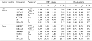
With regards to the sensitivity analysis, the Kling–Gupta statistical criterion (KGE) has been calculated from the output variables of the MIN or MAX simulations as D_sim(t), and from the output variables of the REF simulation as D_ref(t) (Eqs. 19 to 22). For the model calibration and evaluation phase, D_ref(t) is replaced by observed data D_obsf(t). The KGE coefficient is a synthesis of several criteria varying between 1 and −∞ (Gupta et al., 2009), i.e.

$$\begin{array}{}\text{(19)}& {\displaystyle }\mathrm{KGE}=\mathrm{1}\sqrt{(r-\mathrm{1}{)}^{\mathrm{2}}+(\mathit{\alpha }-\mathrm{1}{)}^{\mathrm{2}}+(\mathit{\beta }-\mathrm{1}{)}^{\mathrm{2}}},\end{array}$$

with the linear correlation coefficient (r),

$$\begin{array}{}\text{(20)}& {\displaystyle }r={\displaystyle \frac{\mathrm{\Sigma }\left(\right(D_{\mathrm{sim}}\left(t\right)-\stackrel{\mathrm{‾}}{D_{\mathrm{sim}}})\cdot (D_{\mathrm{ref}}\left(t\right)-\stackrel{\mathrm{‾}}{D_{\mathrm{ref}}}\left)\right)}{\sqrt{\mathrm{\Sigma }\left(D_{\mathrm{sim}}\right(t)-\stackrel{\mathrm{‾}}{D_{\mathrm{sim}}{)}^{\mathrm{2}}}}\cdot \sqrt{\mathrm{\Sigma }\left(D_{\mathrm{ref}}\right(t)-\stackrel{\mathrm{‾}}{D_{\mathrm{ref}}{)}^{\mathrm{2}}}}}},\end{array}$$

with the relative variability (α) represented by the standard deviation:

$$\begin{array}{}\text{(21)}& {\displaystyle }\mathit{\alpha }={\displaystyle \frac{\sqrt{\mathrm{\Sigma }\left(D_{\mathrm{sim}}\right(t)-\stackrel{\mathrm{‾}}{D_{\mathrm{sim}}{)}^{\mathrm{2}}}}}{\sqrt{\mathrm{\Sigma }\left(D_{\mathrm{ref}}\right(t)-\stackrel{\mathrm{‾}}{D_{\mathrm{ref}}{)}^{\mathrm{2}}}}}},\end{array}$$

and with the bias (β),

$$\begin{array}{}\text{(22)}& {\displaystyle }\mathit{\beta }={\displaystyle \frac{\stackrel{\mathrm{‾}}{D_{\mathrm{sim}}}}{\stackrel{\mathrm{‾}}{D_{\mathrm{ref}}}}}.\end{array}$$

The results of the KGE criterion are then presented for each MIN and MAX simulation. For this analysis, the selected model output variables depend on the influence of the parameter on the hydrological processes, namely

• total urban runoff (R_town) and the subsequent total stormwater sewer discharge ($Q_{\mathrm{town}}^{\mathrm{tot}}$); and

• sewer runoff due to soil water infiltration into the sewer network (R_sew).

4.4 Calibration

The TEB-Hydro model is calibrated based on the outcome of the sensitivity analysis. The first few months of the simulation period are systematically excluded, due to model spin-up in order to allow the model to numerically stabilise. Calibration is applied transversely, meaning that the model is calibrated and evaluated over two distinct simulation periods. In this manner, the model is initially calibrated over the first period and then evaluated over the second in following the same process, i.e. inverting the calibration and evaluation periods. The simulations are then compared with the observed total stormwater sewer discharge and, like the sensitivity analysis (Sect. 4.3), the KGE criterion is calculated along with its components.

5 Results and discussion

5.1 Sensitivity analysis

As shown in Table 3, the KGE coefficients for the MIN and MAX simulations, specific to the maximum retention capacity of the surface reservoir of roads (${\mathrm{W}}_{\max ,\mathrm{rd}}^{\mathrm{surf}}$) and roofs (${\mathrm{W}}_{\max ,\mathrm{rf}}^{\mathrm{surf}}$), show little difference with respect to both urban runoff and runoff due to soil water infiltration (Fig. 3a and b). At maximum roof retention capacity, the urban runoff is mainly influenced by minor rainfall events.

Figure 3 Comparison of total urban runoff (R_town) between the reference simulation (REF) and both the MIN simulation (shown in blue) and MAX simulation (red) for the parameters (a) $W_{\max ,\mathrm{rd}}^{\mathrm{surf}}$ (left side) and (b) $W_{\max ,\mathrm{rf}}^{\mathrm{surf}}$ (right side).

Table 3 Statistical criteria (r, α, β, KGE) based on model output variables, as calculated between the MIN and MAX simulations, for each parameter and the reference simulation (REF).

In terms of urban runoff, the model does not show any higher sensitivity to the parameter describing the infiltration rate through the road (I_rd) than to ${\mathrm{W}}_{\max ,\mathrm{rd}}^{\mathrm{surf}}$ and ${\mathrm{W}}_{\max ,\mathrm{rf}}^{\mathrm{surf}}$ (Table 3). Such is not the case however when considering the sewer runoff due to soil water infiltration (R_sew). As the road infiltration rate increases, total urban runoff (R_town) decreases but only for minor rain events (Fig. 4a). Also, moisture rises within the soil layers, thus raising soil water infiltration into the sewer network (Fig. 4b).

Figure 4 (a) Comparison of total urban runoff (R_town) between the reference simulation (REF) and both the MIN simulation (blue) and MAX simulation (red) for parameter I_rd on the left side, and (b) comparison of the sewer runoff due to soil water infiltration (R_sew) between the reference simulation (REF) and the MIN (blue) and MAX (red) simulations for parameter I_rd on the right side.

As expected, the model is more sensitive to the fraction of impervious surfaces connected to the stormwater sewer network (f_con) (Fig. 5). The bias (β) and relative variability (α) (Table 3) reveal different values for MIN and MAX simulations, yet they both lead to the same KGE criterion (Table 3). The variation in the f_con parameter influences total urban runoff as well as sewer runoff due to soil water infiltration. A low connection rate leads to a lower total urban runoff, while a greater parameter value increases the total urban runoff (Fig. 5). The runoff from surfaces not connected to the sewer system feeds infiltration towards the natural surfaces. The amount of infiltrated water in the garden compartment changes with this parameter, thereby influencing soil moisture in all layers and compartments. These values are higher when the fraction of connected surfaces is low and, conversely, lower with a high fraction.

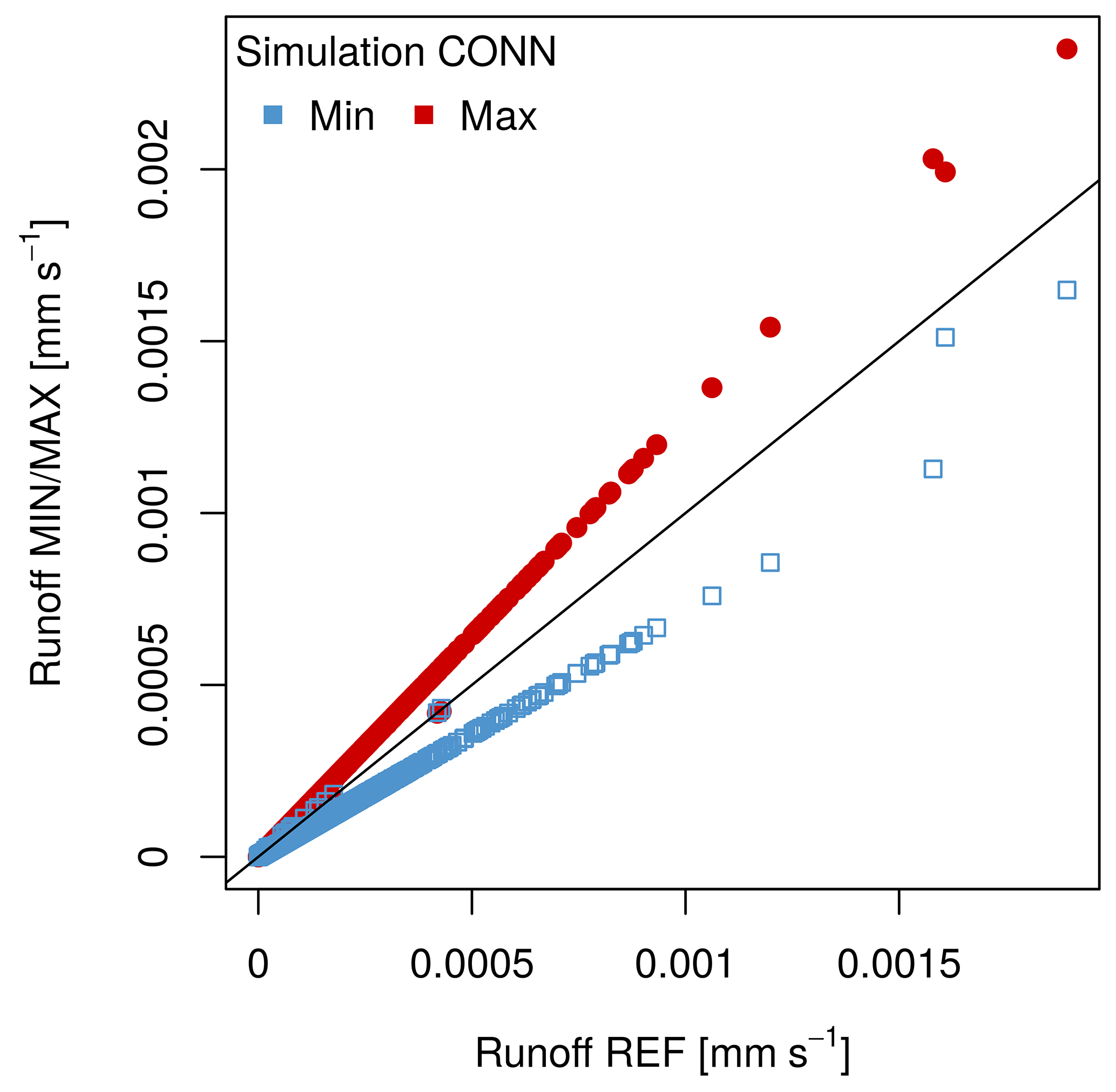
Figure 5 Comparison of total urban runoff (R_town) between the reference simulation (REF) and the MIN (blue) and MAX (red) simulations for parameter f_con.

The calculated KGE values (Table 3) diverge quite a bit between the MIN and MAX simulations for parameters I_p and D_∗ with both output variables, which implies that the model is very sensitive to these parameters. In addition, the results of the factorial design (Fig. 6), based on the calculated direct effects on the maximum sewer discharge due to soil water infiltration, corroborate these findings.

With regard to the parameter describing sewer pipe water tightness (I_p), its increase leads to higher peaks of infiltration into the sewer network (Fig. 7a), yet does not influence the infiltration period. Moreover, the calculated effect of an I_p of $+\mathrm{2.9}{\times }^{-\mathrm{4}}$ signifies an increase in soil water infiltration into the sewer network when transitioning from its low (−1) to its high level (+1) (Fig. 6).

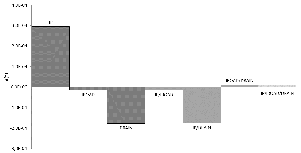
Figure 6 Calculated effects on the model response (R_sew) from parameters I_p, I_rd and D_∗ and their interactions (dark shade of grey: principal effects; medium grey: second-order effects; and light grey: third-order effects).

Figure 7 Comparison of sewer runoff due to soil water infiltration (R_sew) between the reference simulation (REF) and the MIN (blue) and MAX (red) simulations for parameters (a) I_p (left side) and (b) D_∗ (right side).

As for the deep drainage parameter (D_∗), the negative effect (Fig. 6) indicates that infiltration declines with an increasing parameter value. As observed in Fig. 7b, limiting deep drainage to a magnitude of 10 % (MAX) does not generate any significant difference with respect to the reference simulation when assessing sewer discharge due to soil water infiltration. Blocking the deep drainage completely (MIN) however leads to saturating the lower soil layers, thus adding soil water infiltration into the sewer network (Fig. 7b).

As was the case for sewer pipe water tightness (I_p), both the infiltration rate through the road (I_rd) and deep drainage (D_∗) appear to influence sewer drainage due to soil water infiltration, with the effects of their interactions having been calculated and visualised. In this manner, the $I_{\mathrm{p}}/D_{\ast }$ interaction can be highlighted as the most influential of all three first-order interactions (Fig. 6). Also, Fig. 8 effectively displays the correlation between the two parameters (see the two lines running non-parallel to one another), whereas correlations between the other parameters appear to be less significant.

Figure 8 Interactions as a function of the maximum observed sewer runoff due to soil water infiltration during the 1994–1995 winter of the second order between parameters (a) I_p and I_rd; (b) I_p and D_∗; and (c) I_rd and D_∗.

In comparing model sensitivity among the six parameters for total urban runoff and runoff due to soil water infiltration, it can be concluded that the model is less sensitive to changes in parameters ${\mathrm{W}}_{\max ,\mathrm{rd}}^{\mathrm{surf}}$ and ${\mathrm{W}}_{\max ,\mathrm{rf}}^{\mathrm{surf}}$. Four parameters can thus be singled out for calibration:

• the parameter describing sewer pipe water tightness (I_p),

• the infiltration rate through the road (I_rd),

• the fraction of impervious surfaces connected to the sewer network (f_con) and

• the deep drainage (D_∗).

5.2 Model calibration and evaluation

According to the results of the sensitivity analysis, TEB-Hydro needs to be calibrated on four parameters. Yet for both catchment areas, the parameter f_con has been determined as a result of exhaustive field surveys and is therefore well known. Consequently, this parameter will be neglected. Hence, only the three remaining parameters are considered for calibration. Four different values within the predefined range of the sensitivity analysis are tested for each parameter (Table 4). Section 5.1 showed that soil water infiltration into the sewer increases with the I_p value, as opposed to parameters I_rd and D_∗. The range of values has thus been set close to the maximum I_p value and minimum I_rd and D_∗ values. Blocking deep drainage totally would not be a viable option, since in reality soil water is not only drained by artificial sewer systems but can find other pathways within the urban subsoil (groundwater recharge, seepage, etc.). The model is calibrated and evaluated on the total observed stormwater sewer discharge ($Q_{\mathrm{town}}^{\mathrm{tot}}$), as determined from the model outcome variable: total urban runoff (R_town). However, since the drainage capacity of soil water through the sewer network can be extensive in urban areas, the sewer discharge originating from soil water infiltration (Q_sew) has been investigated in detail.

Table 4 Range of values on each parameter tested for use in calibration.

5.2.1 Rezé catchment

As stated above, the calibration step is to be applied transversely. In the Rezé catchment, the calibration and evaluation periods have been compounded by two consecutive hydrological years, i.e. from September 1993 to August 1995, and from September 1995 to August 1997. The KGE criterion results indicate a clear and constant trend for all simulations, independent of either the considered time period (Fig. 9) or the value of parameter D_∗, and this is so for three reasons.

Figure 9 Example of a calculated criterion for the simulation configurations where parameter D_∗ (deep drainage) is limited to 2 % and all other parameters allowed to vary. The KGE criterion, the correlation criterion (r), the variability criterion (α) and the bias (β) for all 16 simulations and for the first (dark grey) and second (light grey) simulation periods are shown.

First, as seen in the example (deep drainage limited to 2 %), all KGE criteria are better for the first period (1993–1995) than for the second (1995–1997) (Fig. 9). This discrepancy between the two simulation periods primarily stems from the KGE criterion component bias (β), which shows a greater value for the second simulation period (Fig. 9). Second, when assessing total stormwater sewer discharge ($Q_{\mathrm{town}}^{\mathrm{tot}}$), the smallest value of I_p achieves a better result than the highest value. Third, the parameter I_rd does not exert a significant influence on the simulated total sewer discharge since the statistical criterion does not vary significantly among its various values. The correlation (r) of simulated and observed discharge peaks is satisfactory, with values of approximately 0.90 for both simulation periods and all simulation configurations (Fig. 9). The model displays a tendency to overestimate the observed total sewer discharge (Fig. 10), more so for the second simulation period, in indicating greater bias (β) across simulations (Fig. 9).

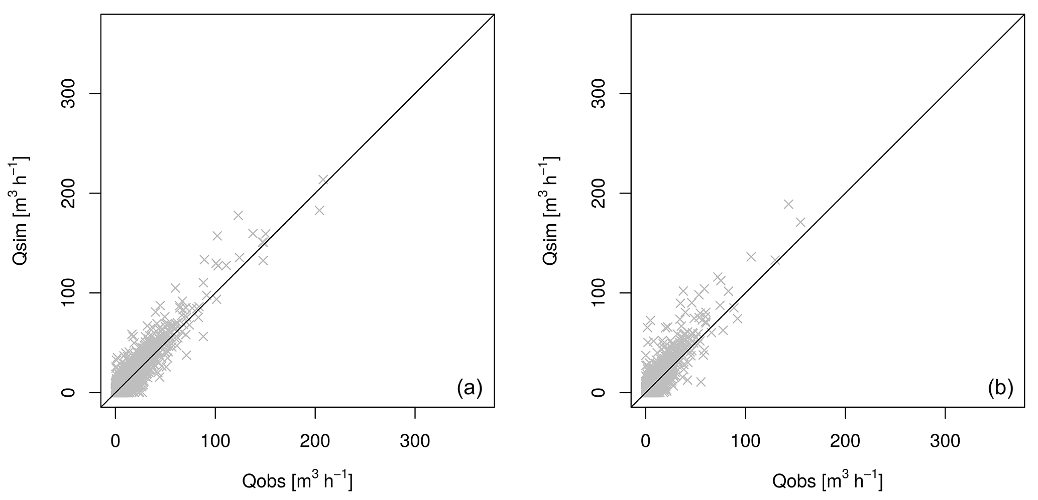
Figure 10 Comparison of simulated and observed total stormwater sewer discharge (m⁻³ h⁻¹) during (a) the first simulation period from September 1993 to August 1995 (left side), and (b) the second simulation period from September 1995 to August 1997 (right side) for simulation 13 and a deep drainage limited to 2 %.

Regardless of the deep drainage values, simulation 13 seems to stand out. The KGE values range between 0.81 and 0.84 for the first period and between 0.66 and 0.68 for the second. In examining both periods separately, simulation 14 appears to perform slightly better during the first period. However, such is not the case during the second period. The degradation in KGE in the second year is mainly related to the higher bias and variability values, most likely caused by the diverse hydrological properties of both simulation periods. For the first period (1993–1995), approximately 1873 mm of precipitation with a very wet 1994–1995 winter can be observed, whereas the second period is much drier, posting just 1302 mm. This trend had indeed already been noticed when coupling ISBA with TOPMODEL (Furusho et al., 2013). The soil representation of ISBA show slow dynamics in the soil water evolution, thus underestimating the water content under wet weather conditions and overestimating it under dry conditions. The model has been calibrated over the first simulation period under wet conditions and evaluated over a drier period. The soil water and, hence, total stormwater discharge are increased with parameters D_∗ and I_p, thus leading to an overestimation.

With regard to total stormwater sewer discharge, the best combination of parameters would consist of setting parameter I_p at 0.09 and I_rd at 10⁻⁵, whereas parameter D_∗ is allowed to vary. Depending on the value of parameter D_∗, the KGE criterion varies between 0.79 and 0.82 over the entire simulation period. We will thus be examining in greater detail the portion of sewer discharge due to soil water infiltration, with parameter D_∗ significantly influencing this process. Berthier (1999) observed a maximum sewer discharge due to soil water infiltration of roughly 0.008 m³ h⁻¹ lm⁻¹ during winter 1994–1995. Accounting for the total sewer length of 1283 m at the Rezé catchment would yield a maximum sewer infiltration rate of approximately 10.3 m³ h⁻¹. Limiting deep drainage to 2 % produces a simulated discharge peak of 4.8 m³ h⁻¹ during this period (Fig. 11a), which is much less than the observed findings. In examining the simulation with a limited deep drainage (D_∗) of 1 %, the observed discharge peak becomes significantly overestimated at 27 m³ h⁻¹ (Fig. 11b). In the aim of evaluating the model as well on the sewer discharge due to soil water infiltration, deep drainage should be limited to somewhere between 1 % and 2 %.

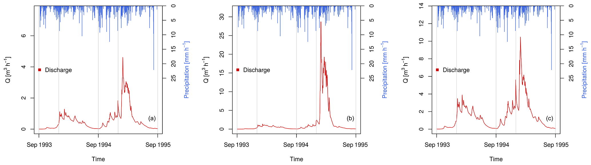
Figure 11 Simulated sewer discharge due to soil water infiltration (m⁻³ h⁻¹) during the first simulation period 1993–1995 based on the combination of parameters I_p set at 0.09 and I_rd set at 10⁻⁵ and (a) D_∗ limited to 2 %, (b) D_∗ limited to 1 % and (c) based on the combination of parameters I_p set at 0.3 and I_rd set at 10⁻⁵, with a D_∗ value limited to 2 %.

Another option would consist of focusing on the I_p parameter since the sensitivity analysis also revealed its influence on the process of soil water infiltration into the sewer. As stated above, raising the value of I_p is beneficial for the infiltration rate. Hence, simulation 14 would be more suitable, as I_p has been set at 0.3 while I_rd remains at 10⁻⁵. In conjunction with deep drainage limited to 2 %, the maximum sewer discharge due to soil water infiltration during winter 1994–1995 equals approximately 10.6 m³ h⁻¹, which is close to the observed maximum discharge (Fig. 11c). For this combination of parameters (i.e. I_p=0.3, $I_{\mathrm{rd}}={\mathrm{10}}^{-\mathrm{5}}$, $D_{\ast }=\mathrm{2}$), the KGE criterion based on total sewer discharge is slightly better, as is the case for simulation 13, with a value of 0.86 for the first period. Such is not the case however for the second period, with a value dropping to 0.57.

5.2.2 Pin Sec catchment

For the Pin Sec catchment, the period between September 2010 and August 2011 has been compared to the period from September 2011 to August 2012, and vice versa. As was the case with the Rezé catchment, the same trends and patterns can be observed independently of the simulation periods and configurations. Simulation 13 is once again cited as the best set of parameters, with a KGE criterion equal to 0.79 over the entire period. Parameter I_p should thus be set at 0.09 and I_rd at 10⁻⁵, whereas D_∗ remains variable.

5.2.3 General discussion

In terms of calibration and evaluation processes, TEB-Hydro exhibits the tendency to overestimate the observed total stormwater sewer discharge. This skewing can be explained by the decision to set parameter f_con at its documented value rather than calibrating the model on it. This parameter is indeed the one exerting a predominant influence on total stormwater sewer discharge, since it directly influences the surface runoff of impervious surfaces. When calibrating the model on total stormwater sewer discharge, it is thus essential to take this parameter into account even if it is well known. On the contrary, such is not the case for the parameters I_rd and D_∗, which exercise little influence over this process. Evaluating the model from the standpoint of sewer discharge due to soil water infiltration however requires a more detailed consideration of I_p and D_∗. The water exchange processes taking place between the urban subsoil and both the natural and sewer network are critical processes in urban areas. As shown above, the model is very sensitive to these processes and comparing them to observed findings can improve the simulated urban water budget, yet experimental data on such fluxes are indeed rare.

For both catchments, the statistical criteria indicate the same trend across all simulation configurations and periods, with a better KGE for the wetter periods. The best simulation configuration is the same irrespective of calibrating the model on the first or second period, with the exception of simulation 14. It thus proves necessary to apply the model more extensively in regions with different meteorological patterns in order to investigate whether the model could operate under different weather conditions (dry and wet periods), as this would be an essential condition for projection applications. The same simulation configuration yields the best results for both the Rezé and Pin Sec catchments. Considering their differences in terms of soil texture and urban patterns (i.e. mean building height), this result is encouraging for work at the city scale, with spatial heterogeneity no longer constituting an obstacle.

6 Conclusions

The objective of this study has been to contribute to developing a complete urban hydro-microclimate model and testing the ability of this model to replicate hydrological processes. This goal has been achieved given that the representation of hydrological processes in the TEB-Veg model (Lemonsu et al., 2012a) has been extended and refined. The new model version, called TEB-Hydro, has been developed by taking a detailed representation of the urban subsoil into account. This step has allowed for horizontal interactions of soil moisture between the urban subsoil of built-up and natural surfaces within a single grid cell. Furthermore, soil water drainage via the sewer network has been introduced into the road compartment of the TEB-Hydro model. Deep drainage, which normally supplies the base flow of the natural river network, has been limited to favouring humidification of the lower soil layers. This condition results in more realistic infiltration patterns in the sewer network under urban conditions. A sensitivity analysis has been performed with the aim of better understanding the influences of model parameters on these processes while identifying the parameters to serve for calibration purposes. Six parameters were investigated, with four of them appearing to significantly influence model output in terms of total sewer discharge and the portion of discharge caused by soil water infiltration, namely parameter I_p describing the sewer pipe water tightness, the road infiltration rate (I_rd), the fraction of impervious surfaces connected to the sewer network (f_con) and parameter D_∗ to enable limiting deep drainage out of the urban subsoil.

TEB-Hydro was then applied to two small residential catchments located close to the city of Nantes (France). In both cases, the model was calibrated and evaluated on the observed stormwater sewer discharge, in displaying the same hydrological behaviour. Total stormwater sewer discharge is consistently being overestimated, independently of simulation period and configuration. Considering parameter f_con as a calibration element allows tackling this problem. The model seems to function better under wet conditions, with improved KGE results. In assessing the entire simulation period for both catchments, the same parameter configuration stands out, independently of meteorological and local physical conditions, thus implying that the model is running in a coherent and steady manner. This finding would need to be confirmed by applying the model to several catchment areas outside of Nantes. In conclusion, the evaluation outcomes set forth herein are encouraging for model application at the city scale for purposes of projecting global change.

Lastly, a more detailed representation of the urban subsoil and its hydrological pattern enhances the model's urban water budget. Given that water and energy budgets are coupled, it is likely that the energy budget of this model is being influenced at the same time. A research project now underway entails investigating energy patterns, like latent and sensible heat fluxes, alongside the hydrological processes.

Appendix A: List of symbols

Q∗	net all-wave radiation (W m−2)
QF	anthropogenic heat flux (W m−2)
QH	sensible heat flux (W m−2)
QE	latent heat flux (W m−2)
ΔQS	heat flux storage (W m−2)
ΔQA	net advection heat flux (W m−2)
P	total precipitation (kg m−2 s−1)
I	water generated from anthropogenic activities (irrigation) (kg m−2 s−1)
E∗	evapotranspiration over * compartment (kg m−2 s−1)
R	total runoff (kg m−2 s−1)
D∗	deep drainage over * compartment (kg m−2 s−1)
ΔW	variation in water storage both on the surface and in the ground during the simulation period (kg m−2 s−1)
Lv	latent heat of vaporisation (J kg−1)
T∗	transfer
$W_{\ast }^{\mathrm{surf}}$	surface retention capacity over * compartment (mm)
$W_{max,\ast }^{\mathrm{surf}}$	maximum surface retention capacity over * compartment (mm)
I∗	surface water infiltration rate of * compartment (m s−1)
$R_{\ast }^{\mathrm{surf}}$	surface runoff connected to the sewer network for * compartment (mm s−1)
fcon	effective connected impervious area fraction (–)
Rsew	runoff in the sewer network due to soil water infiltration (mm s−1)
$R_{\ast }^{\mathrm{subsurf}}$	subsurface runoff from * compartment (mm s−1)
$W_{\ast }^{\mathrm{gr}}$	soil moisture content before horizontal balancing over * compartment (m3 m−3)
$W_{\ast }^{\mathrm{gr}{,}^{\prime }}$	soil moisture content after horizontal balancing over * compartment (m3 m−3)
$\stackrel{\mathrm{‾}}{W^{\mathrm{gr}}}$	mean soil moisture content of all compartments before balancing (m3 m−3)
τ	time constant for 1 day(s)
$\frac{\stackrel{\mathrm{‾}}{K_{\mathrm{sat}}}}{K_i}$	ratio of the mean hydraulic conductivity at saturation of all three compartments to the hydraulic conductivity of each compartment (–)
dt	numerical time step of the model(s)
f∗	surface area fraction of * compartment (–)

Ip	parameter representing the water tightness of the sewer pipe (–)
Dsew	sewer density within a single grid cell (–), expressed by the ratio of the total sewer length in one grid cell (m) to the maximum total sewer length in a single grid cell of the entire study site (m)
$W_{\ast }^{\mathrm{gr},n}$	soil moisture content of the last layer n of * compartment (m3 m−3)
$W_{\ast }^{\mathrm{gr},\mathrm{flux},n}$	soil moisture content derived from the outgoing water flux of * compartment (m3 m−3)
Crech	coefficient of recharge (–) in order to limit deep drainage
dn	thickness of the last layer
ρ	water density (kg m−3)
$W_{\ast ,\mathrm{sat}}^{\mathrm{gr},i}$	soil moisture content at saturation of * compartment (m3 m−3)
$W_{\ast }^{\mathrm{gr},i{,}^{\prime }}$	soil moisture content in layer i after update of * compartment (m3 m−3)
$W_{\ast }^{\mathrm{gr},i}$	soil moisture content in layer i before update of * compartment (m3 m−3)
di	layer thicknesses of layer i (–)
$R_{\ast }^{\mathrm{subsurf}{,}^{\prime }}$	subsurface runoff after update of * compartment (mm s−1)
$R_{\ast }^{\mathrm{subsurf}}$	subsurface runoff before update of * compartment (mm s−1)
e(A)	principal effect of a parameter called A (–)
e(AB)	effect of the interaction between two different parameters A and B (–)
${\stackrel{\mathrm{‾}}{y}}_{\ast +}$	mean response of all combinations where the parameter or interaction of two parameters is at its high level (+1) (–)
${\stackrel{\mathrm{‾}}{y}}_{\ast -}$	mean response of all combinations where the parameter or interaction of two parameters is at its low level (−1) (–)
$Q_{\mathrm{town}}^{\mathrm{tot}}$	total stormwater sewer discharge (m3 h−1) derived from total urban runoff (Rtown) (m3 h−1)
Qsew	sewer discharge due to soil water infiltration (m3 h−1) derived from sewer runoff (Rsew) (m3 h−1)
KGE	Kling–Gupta statistical criterion (–)
r	correlation (–)
α	variability (–)
β	bias (–)
Dsim(t)	output variables of MIN and MAX simulations (kg m−2 s−1)
Dref(t)	output variables of the REF simulation; this symbol is replaced by observed data Dobsf(t) for purposes of model calibration and the evaluation phase (kg m−2 s−1)

with subscripts * standing for
rf	roof
rd	road
gdn	garden
bld	building
con	connection
veg	vegetation
gr	bare ground surface
s	sublimation from snow
sat	saturation
sew	sewer
rech	recharge
max	maximum
sim	simulation
ref	reference
obs	observation
v	vertical
h	horizontal
with superscripts * standing for
tot	total
gr	ground
surf	surface
subsurf	subsurface
i	layer number
n	number of last layer