Development and evaluation of a variably saturated flow model in the global E3SM Land Model (ELM) version 1.0

Improving global-scale model representations of near-surface soil moisture and groundwater hydrology is important for accurately simulating terrestrial processes and predicting climate change effects on water resources. Most existing land surface models, including the default E3SM Land Model (ELMv0), which we modify here, routinely employ different formulations for water transport in the vadose and phreatic zones. Clark et al. (2015) identified a variably saturated Richards equation flow model as an important capability for improving simulation of coupled soil moisture and shallow groundwater dynamics. In this work, we developed the Variably Saturated Flow Model (VSFM) in ELMv1 to unify the treatment of soil hydrologic processes in the unsaturated and saturated zones. VSFM was tested on three benchmark problems and results were evaluated against observations and an existing benchmark model (PFLOTRAN). The ELMv1-VSFM's subsurface drainage parameter, f_d, was calibrated to match an observationally constrained and spatially explicit global water table depth (WTD) product. Optimal spatially explicit f_d values were obtained for 79 % of global 1.9^∘ × 2.5^∘ grid cells, while the remaining 21 % of global grid cells had predicted WTD deeper than the observationally constrained estimate. Comparison with predictions using the default f_d value demonstrated that calibration significantly improved predictions, primarily by allowing much deeper WTDs. Model evaluation using the International Land Model Benchmarking package (ILAMB) showed that improvements in WTD predictions did not degrade model skill for any other metrics. We evaluated the computational performance of the VSFM model and found that the model is about 30 % more expensive than the default ELMv0 with an optimal processor layout. The modular software design of VSFM not only provides flexibility to configure the model for a range of problem setups but also allows for building the model independently of the ELM code, thus enabling straightforward testing of the model's physics against other models.

1 Introduction

Groundwater, which accounts for 30 % of freshwater reserves globally, is a vital human water resource. It is estimated that groundwater provides 20–30 % of global freshwater withdrawals (Petra, 2009; Zektser and Evertt, 2004), and that irrigation accounts for ∼70 % of these withdrawals (Siebert et al., 2010). Climate change is expected to impact the quality and quantity of groundwater in the future (Alley, 2001). As temporal variability in precipitation and surface water increases in the future due to climate change, reliance on groundwater as a source of fresh water for domestic, agriculture, and industrial use is expected to increase (Taylor et al., 2013).

Local environmental conditions modulate the impact of rainfall changes on groundwater resources. For example, high-intensity precipitation in humid areas may lead to a decrease in groundwater recharge (due to higher surface runoff), while arid regions are expected to see gains in groundwater storage (as infiltrating water quickly travels deep into the ground before it can be lost to the atmosphere; Kundzewicz and Doli, 2009). Although global climate models predict changes in precipitation over the next century (Marvel et al., 2017), few global models that participated in the recent Coupled Model Intercomparison Project (CMIP5; Taylor et al., 2012) were able to represent global groundwater dynamics accurately (e.g., Swenson and Lawrence, 2014)

Modeling studies have also investigated impacts, at watershed to global scales, on future groundwater resources associated with land-use (LU) and land-cover (LC) change (Dams et al., 2008) and ground water pumping (Ferguson and Maxwell, 2012; Leng et al., 2015). Dams et al. (2008) predicted that LU changes would result in a small mean decrease in subsurface recharge and large spatial and temporal variability in groundwater depth for the Kleine Nete basin in Belgium. Ferguson and Maxwell (2012) concluded that groundwater-fed irrigation impacts on water exchanges with the atmosphere and groundwater resources can be comparable to those from a 2.5 ^∘C increase in air temperature for the Little Washita basin in Oklahoma, USA. By performing global simulations of climate change scenarios using CLM4, Leng et al. (2015) concluded that the water source (i.e., surface or groundwater) used for irrigation depletes the corresponding water source while increasing the storage of the other water source. Recently, Leng et al. (2017) showed that the irrigation method (drip, sprinkler, or flood) has impacts on water balances and water use efficiency in global simulations.

Groundwater models are critical for developing understanding of groundwater systems and predicting impacts of climate (Green et al., 2011). Kollet and Maxwell (2008) identified critical zones, i.e., regions within the watershed with water table depths between 1 and 5 m, where the influence of groundwater dynamics was largest on surface energy budgets. Numerical studies have demonstrated impacts of groundwater dynamics on several key Earth system processes, including soil moisture (Chen and Hu, 2004; Liang et al., 2003; Salvucci and Entekhabi, 1995; Yeh and Eltahir, 2005), runoff generation (Levine and Salvucci, 1999; Maxwell and Miller, 2005; Salvucci and Entekhabi, 1995; Shen et al., 2013), surface energy budgets (Alkhaier et al., 2012; Niu et al., 2017; Rihani et al., 2010; Soylu et al., 2011), land–atmosphere interactions (Anyah et al., 2008; Jiang et al., 2009; Leung et al., 2011; Yuan et al., 2008), vegetation dynamics (Banks et al., 2011; Chen et al., 2010), and soil biogeochemistry (Lohse et al., 2009; Pacific et al., 2011).

Recognizing the importance of groundwater systems on terrestrial processes, groundwater models of varying complexity have been implemented in land surface models (LSMs) in recent years. Groundwater models in current LSMs can be classified into four categories based on their governing equations. Type-1 models assume a quasi-steady state equilibrium of the soil moisture profile above the water table (Hilberts et al., 2005; Koster et al., 2000; Walko et al., 2000). Type-2 models use a θ-based (where θ is the water volume content) Richards equation in the unsaturated zone coupled with a lumped unconfined aquifer model in the saturated zone. Examples of one-dimensional Type-2 models include Liang et al. (2003), Yeh and Eltahir (2005), Niu et al. (2007), and Zeng and Decker (2009). Examples of quasi-three-dimensional Type-2 models are York et al. (2002), Fan et al. (2007), Miguez-Macho et al. (2007), and Shen et al. (2013). Type-3 models include a three-dimensional representation of subsurface flow based on the variably saturated Richards equation (Maxwell and Miller, 2005; Tian et al., 2012). Type-3 models employ a unified treatment of hydrologic processes in the vadose and phreatic zones but lump changes associated with water density and unconfined aquifer porosity into a specific storage term. The fourth class (Type-4) of subsurface flow and reactive transport models (e.g., PFLOTRAN, Hammond and Lichtner, 2010; TOUGH2, Pruess et al., 1999; and STOMP, White and STOMP, 2000) combine a water equation of state (EoS) and soil compressibility with the variably saturated Richards equation. Type-4 models have not been routinely coupled with LSMs to address climate change relevant research questions. Clark et al. (2015) summarized that most LSMs use different physics formulations for representing hydrologic processes in saturated and unsaturated zones. Additionally, Clark et al. (2015) identified the incorporation of variably saturated hydrologic flow models (i.e., Type-3 and Type-4 models) in LSMs as a key opportunity for future model development that is expected to improve simulation of coupled soil moisture and shallow groundwater dynamics.

The Energy, Exascale, Earth System Model (E3SM) is a new Earth system modeling project sponsored by the US Department of Energy (E3SM Project, 2018). The E3SM model started from the Community Earth System Model (CESM) version 1_3_beta10 (Oleson et al., 2013). Specifically, the initial version (v0) of the E3SM Land Model (ELM) was based off the Community Land Model's (CLM's) tag 4_5_71. ELMv0 uses a Type-2 subsurface hydrology model based on Zeng and Decker (2009). In this work, we developed in ELMv1 the Type-4 Variably Saturated Flow Model (VSFM) to provide a unified treatment of soil hydrologic processes within the unsaturated and saturated zones. The VSFM formulation is based on the isothermal, single phase, variably saturated (RICHARDS) flow model within PFLOTRAN (Hammond and Lichtner, 2010). While PFLOTRAN is a massively parallel, three-dimensional subsurface model, the VSFM is a serial, one-dimensional model that is appropriate for climate-scale applications.

This paper is organized into several sections: (1) a brief review of the ELMv0 subsurface hydrology model; (2) an overview of the VSFM formulation integrated in ELMv1; (3) an application of the new model formulation to three benchmark problems; (4) development of a subsurface drainage parameterization necessary to predict global water table depths (WTDs) comparable to recently released observationally constrained estimates; (5) comparison of ELMv1 global simulations with the default subsurface hydrology model and VSFM against multiple observations using the International Land Model Benchmarking package (ILAMB; Hoffman et al., 2017); and (6) a summary of major findings.

2 Methods

2.1 Current model formulation

Water flow in the unsaturated zone is often described by the θ-based Richards equation:

$$\begin{array}{}\text{(1)}& {\displaystyle \frac{\partial \mathit{\theta }}{\partial t}}=-\mathrm{\nabla }\cdot \mathbf{q}-Q,\end{array}$$

where θ (m³ of water m⁻³ of soil) is the volumetric soil water content, t (s) is time, q (m s⁻¹) is the Darcy water flux, and Q (m³ of water m⁻³ of soil s⁻¹) is a soil moisture sink term. The Darcy flux, q, is given by

$$\begin{array}{}\text{(2)}& {\displaystyle }\mathit{q}=-K\mathrm{\nabla }(\mathit{\psi }+z),\end{array}$$

where K (m s⁻¹) is the hydraulic conductivity, z (m) is height above some datum in the soil column and ψ (m) is the soil matric potential. The hydraulic conductivity and soil matric potential are modeled as non-linear functions of volumetric soil moisture following Clapp and Hornberger (1978):

$$\begin{array}{}\text{(3)}& {\displaystyle }& {\displaystyle }K={\mathrm{\Theta }}_{\mathrm{ice}}{K}_{\mathrm{sat}}{\left({\displaystyle \frac{\mathit{\theta }}{{\mathit{\theta }}_{\mathrm{sat}}}}\right)}^{\mathrm{2}B+\mathrm{3}},\text{(4)}& {\displaystyle }& {\displaystyle }\mathit{\psi }={\mathit{\psi }}_{\mathrm{sat}}{\left({\displaystyle \frac{\mathit{\theta }}{{\mathit{\theta }}_{\mathrm{sat}}}}\right)}^{-B},\end{array}$$

where K_sat (m s⁻¹) is saturated hydraulic conductivity, ψ_sat (m) is saturated soil matric potential, B is a linear function of percentage clay and organic content (Oleson et al., 2013), and Θ_ice is the ice impedance factor (Swenson et al., 2012). ELMv0 uses the modified form of the Richards equation of Zeng and Decker (2009) that computes Darcy flux as

$$\begin{array}{}\text{(5)}& {\displaystyle }\mathbf{q}=-K\mathrm{\nabla }(\mathit{\psi }+z-C),\end{array}$$

where C is a constant hydraulic potential above the water table, z_∇, given as

$$\begin{array}{}\text{(6)}& {\displaystyle }C={\mathit{\psi }}_{\mathrm{E}}+z={\mathit{\psi }}_{\mathrm{sat}}{\left({\displaystyle \frac{{\mathit{\theta }}_{\mathrm{E}}\left(z\right)}{{\mathit{\theta }}_{\mathrm{sat}}}}\right)}^{-B}+z={\mathit{\psi }}_{\mathrm{sat}}+z_{\mathrm{\nabla }},\end{array}$$

where ψ_E (m) is the equilibrium soil matric potential, z (m) is height above a reference datum, θ_E (m³ m⁻³) is volumetric soil water content at equilibrium soil matric potential, and z_∇ (m) is the height of the water table above a reference datum. ELMv0 uses a cell-centered finite volume spatial discretization and backward Euler implicit time integration. By default, ELMv0's vertical discretization of a soil column yields 15 soil layers of exponentially varying soil thicknesses that reach a depth of 42.1 m Only the first 10 soil layers (or top 3.8 m of each soil column) are hydrologically active, while thermal processes are resolved for all 15 soil layers. The nonlinear Darcy flux is linearized using Taylor series expansion and the resulting tri-diagonal system of equations is solved by LU factorization.

Flow in the saturated zone is modeled as an unconfined aquifer below the soil column based on the work of Niu et al. (2007). Exchange of water between the soil column and unconfined aquifer depends on the location of the water table. When the water table is below the last hydrologically active soil layer in the column, a recharge flux from the last soil layer replenishes the unconfined aquifer. A zero-flux boundary condition is applied to the last hydrologically active soil layer when the water table is within the soil column. The unconfined aquifer is drained by a flux computed based on the SIMTOP scheme of Niu et al. (2007) with modifications to account for frozen soils (Oleson et al., 2013).

2.2 New VSFM model formulation

In the VSFM formulation integrated in ELMv1, we use the mass conservative form of the variably saturated subsurface flow equation (Farthing et al., 2003; Hammond and Lichtner, 2010; Kees and Miller, 2002):

$$\begin{array}{}\text{(7)}& {\displaystyle \frac{\partial \left(\mathit{\varphi }{s}_{\mathrm{w}}\mathit{\rho }\right)}{\partial t}}=-\mathrm{\nabla }\cdot \left(\mathit{\rho }\mathbf{q}\right)-Q,\end{array}$$

where ϕ (m³ m⁻³) is the soil porosity, s_w (-) is saturation, ρ (kg m⁻³) is water density, q (m s⁻¹) is the Darcy velocity, and Q (kg m⁻³ s⁻¹) is a water sink. We restrict our model formulation to a one-dimensional system and the flow velocity is defined by Darcy's law:

$$\begin{array}{}\text{(8)}& {\displaystyle }\mathbf{q}=-{\displaystyle \frac{k{k}_{\mathrm{r}}}{\mathit{\mu }}}\mathrm{\nabla }(P+\mathit{\rho }gz),\end{array}$$

where k (m²) is intrinsic permeability, k_r (-) is relative permeability, μ (Pa s) is viscosity of water, P (Pa) is pressure, g (m s⁻²) is the acceleration due to gravity, and z (m) is elevation above some datum in the soil column.

In order to close the system, a constitutive relationship is used to express saturation and relative permeability as a function of soil matric pressure. Analytic water retention curves (WRCs) are used to model effective saturation (s_e)

$$\begin{array}{}\text{(9)}& {\displaystyle }{s}_{\mathrm{e}}=\left({\displaystyle \frac{s_{\mathrm{w}}-s_{\mathrm{r}}}{\mathrm{1}-s_{\mathrm{r}}}}\right),\end{array}$$

where s_w is saturation and s_r is residual saturation. We have implemented Brooks and Corey (1964; Eq. 10) and van Genuchten (1980; Eq. 11) WRCs:

$$\begin{array}{}\text{(10)}& {\displaystyle }& {\displaystyle }{s}_{\mathrm{e}}=\left\{\begin{array}{ll}{\left({\displaystyle \frac{-P_{\mathrm{c}}}{P_{\mathrm{c}}^{\mathrm{0}}}}\right)}^{-\mathit{\lambda }}& \text{if}{P}_{\mathrm{c}}<P_{\mathrm{c}}^{\mathrm{0}},\\ \mathrm{1}& \text{if}{P}_{\mathrm{c}}\ge P_{\mathrm{c}}^{\mathrm{0}},\end{array}\right.\text{(11)}& {\displaystyle }& {\displaystyle }{s}_{\mathrm{e}}=\left\{\begin{array}{ll}{\left[\mathrm{1}+{\left(\mathit{\alpha }\left|P_{\mathrm{c}}\right|\right)}^n\right]}^{-m}& \text{if}{P}_{\mathrm{c}}<\mathrm{0},\\ \mathrm{1}& \text{if}{P}_{\mathrm{c}}\ge \mathrm{0},\end{array}\right.\end{array}$$

where P_c (Pa) is the capillary pressure, $P_{\mathrm{c}}^{\mathrm{0}}$ (Pa) is the air entry pressure, α (Pa⁻¹) is inverse of the air entry pressure, λ (-) is the exponent in the Brooks and Corey parameterization, and n (-) and m (-) are the van Genuchten parameters. The capillary pressure is computed as $P_{\mathrm{c}}=P-P_{\mathrm{ref}}$ where P_ref is $P_{\mathrm{c}}^{\mathrm{0}}$ for Brooks and Corey WRC and typically the atmospheric pressure (=101 325 Pa) is used for the van Genuchten WRC. In addition, a smooth approximation of Eqs. (10) and (11) was developed to facilitate convergence of the nonlinear solver (Appendix A). Relative soil permeability was modeled using the Mualem (1976) formulation:

$$\begin{array}{}\text{(12)}& {\displaystyle }{\mathit{\kappa }}_{\mathrm{r}}\left(s_{\mathrm{e}}\right)=\left\{\begin{array}{l}{s}_{\mathrm{e}}^{\mathrm{0.5}}\left[\mathrm{1}-{\left(\mathrm{1}-s_{\mathrm{e}}^{\mathrm{1}/m}\right)}^m\right]\text{if}P<P_{\mathrm{ref}},\\ \mathrm{1}\text{if}P\ge P_{\mathrm{ref}},\end{array}\right.\end{array}$$

where $m=\mathrm{1}-\mathrm{1}/n$. Lastly, we used an EoS for water density, ρ, that is a nonlinear function of liquid pressure, P, and liquid temperature, T, given by Tanaka et al. (2001):

$$\begin{array}{ll}{\displaystyle }\mathit{\rho }\left(P,T\right)& {\displaystyle }=\left[\mathrm{1}+\left(k_{\mathrm{0}}+k_{\mathrm{1}}T+k_{\mathrm{2}}{T}^{\mathrm{2}}\right)\left(P-P_{\mathrm{ref}}\right)\right]\\ \text{(13)}& {\displaystyle }& {\displaystyle }{a}_{\mathrm{5}}\left[\mathrm{1}-{\displaystyle \frac{{\left(T+a_{\mathrm{1}}\right)}^{\mathrm{2}}\left(T+a_{\mathrm{2}}\right)}{a_{\mathrm{3}}\left(T+a_{\mathrm{4}}\right)}}\right],\end{array}$$

where

$$\begin{array}{ll}{\displaystyle }& {\displaystyle }{k}_{\mathrm{0}}=\mathrm{50.74}\times {\mathrm{10}}^{-\mathrm{11}}\left({\mathrm{Pa}}^{-\mathrm{1}}\right),\\ {\displaystyle }& {\displaystyle }{k}_{\mathrm{1}}=-\mathrm{0.326}\times {\mathrm{10}}^{-\mathrm{11}}\left({\mathrm{Pa}}^{-\mathrm{1}}{\mathrm{C}}^{-\mathrm{1}}\right),\\ {\displaystyle }& {\displaystyle }{k}_{\mathrm{2}}=\mathrm{0.00416}\times {\mathrm{10}}^{-\mathrm{11}}\left({\mathrm{Pa}}^{-\mathrm{1}}{\mathrm{C}}^{\mathrm{2}}\right),\\ {\displaystyle }& {\displaystyle }{a}_{\mathrm{1}}=-\mathrm{3.983035}\left(\mathrm{C}\right),\\ {\displaystyle }& {\displaystyle }{a}_{\mathrm{2}}=\mathrm{301.797}\left(\mathrm{C}\right),\\ {\displaystyle }& {\displaystyle }{a}_{\mathrm{3}}=\mathrm{522558.9}\left({\mathrm{C}}^{-\mathrm{2}}\right),\\ {\displaystyle }& {\displaystyle }{a}_{\mathrm{4}}=\mathrm{69.34881}\left(\mathrm{C}\right),\\ {\displaystyle }& {\displaystyle }{a}_{\mathrm{5}}=\mathrm{999.974950}\left(\mathrm{kg}{\mathrm{m}}^{-\mathrm{3}}\right).\end{array}$$

The sink of water due to transpiration from a given plant functional type (PFT) is vertically distributed over the soil column based on area and root fractions of the PFT. The top soil layer has an additional flux associated with balance of infiltration and soil evaporation. The subsurface drainage flux is applied proportionally to all soil layers below the water table. Details on the computation of water sinks are given in Oleson et al. (2013). Unlike the default subsurface hydrology model, the VSFM is applied over the full soil depth (in the default model, 15 soil layers). The VSFM model replaces both the θ-based Richards equation and the unconfined aquifer of the default model and uses a zero-flux lower boundary condition. In the VSFM model, water table depth is diagnosed based on the vertical soil liquid pressure profile. Like the default model, drainage flux is computed based on the modified SIMTOP approach and is vertically distributed over the soil layers below the water table.

2.2.1 Discrete equations

We use a cell-centered finite volume discretization to decompose the spatial domain, Ω, into N non-overlapping control volumes, Ω_n, such that $\mathrm{\Omega }={\cup }_{n=\mathrm{1}}^N{\mathrm{\Omega }}_i$ and Γ_n represents the boundary of the nth control volume. Applying a finite volume integral to Eq. (7) and the divergence theorem yields

$$\begin{array}{}\text{(14)}& {\displaystyle \frac{\partial }{\partial t}}\underset{{\mathrm{\Omega }}_n}{\int }\left(\mathit{\varphi }{s}_{\mathrm{w}}\mathit{\rho }\right)\mathrm{d}V=-\underset{{\mathrm{\Gamma }}_n}{\int }\left(\mathit{\rho }\mathbf{q}\right)\cdot \mathrm{d}\mathbf{A}-\underset{{\mathrm{\Omega }}_n}{\int }Q\mathrm{d}V.\end{array}$$

The discretized form of the left-hand-side term and first term on the right-hand side of Eq. (14) are approximated as

$$\begin{array}{}\text{(15)}& {\displaystyle \frac{\partial }{\partial t}}\underset{{\mathrm{\Omega }}_n}{\int }\left(\mathit{\varphi }{s}_{\mathrm{w}}\mathit{\rho }\right)\mathrm{d}V\approx \left({\displaystyle \frac{d}{\mathrm{d}t}}\left(\mathit{\varphi }{s}_{\mathrm{w}}\mathit{\rho }\right)\right)V_n,\text{(16)}& {\displaystyle }\underset{{\mathrm{\Gamma }}_n}{\int }\left(\mathit{\rho }\mathbf{q}\right)\cdot \mathrm{d}\mathbf{A}\approx \sum _{n^{\prime }}{\left(\mathit{\rho }\mathbf{q}\right)}_{nn{}^{\prime }}\cdot {\mathbf{A}}_{nn{}^{\prime }},\end{array}$$

where ${\mathbf{A}}_{nn{}^{\prime }}$ (m²) is the common face area between the nth and n^′th control volumes. After substituting Eqs. (15) and (16) in Eq. (14), the resulting ordinary differential equation for the variably saturated flow model is

$$\begin{array}{}\text{(17)}& {\displaystyle }\left({\displaystyle \frac{d}{\text{d}t}}\left(\mathit{\varphi }{s}_{\mathrm{w}}\mathit{\rho }\right)\right)V_n=-\sum _{n^{\prime }}{\left(\mathit{\rho }\mathbf{q}\right)}_{nn{}^{\prime }}\cdot {\mathbf{A}}_{nn{}^{\prime }}-Q_n{V}_n.\end{array}$$

We perform temporal integration of Eq. (17) using the backward-Euler scheme:

$$\begin{array}{ll}{\displaystyle }& {\displaystyle }\left({\displaystyle \frac{{\left(\mathit{\varphi }{s}_{\mathrm{w}}\mathit{\rho }\right)}_n^{t+\mathrm{1}}-{\left(\mathit{\varphi }{s}_{\mathrm{w}}\mathit{\rho }\right)}_n^t}{\mathrm{\Delta }t}}\right)V_n=-\sum _{n^{\prime }}{\left(\mathit{\rho }\mathbf{q}\right)}_{n{n}^{\prime }}^{t+\mathrm{1}}\cdot {\mathbf{A}}_{nn{}^{\prime }}.\\ \text{(18)}& {\displaystyle }& {\displaystyle }-Q_n^{t+\mathrm{1}}{V}_n\end{array}$$

Rearranging terms of Eq. (18) results in a nonlinear equation for the unknown pressure at time step t+1 as

$$\begin{array}{ll}{\displaystyle }& {\displaystyle }\left({\displaystyle \frac{{\left(\mathit{\varphi }{s}_{\mathrm{w}}\mathit{\rho }\right)}_n^{t+\mathrm{1}}-{\left(\mathit{\varphi }{s}_{\mathrm{w}}\mathit{\rho }\right)}_n^t}{\mathrm{\Delta }t}}\right)V_n+\sum _{n^{\prime }}{\left(\mathit{\rho }\mathbf{q}\right)}_{n{n}^{\prime }}^{t+\mathrm{1}}\cdot {\mathbf{A}}_{nn{}^{\prime }}\\ \text{(19)}& {\displaystyle }& {\displaystyle }+Q_n^{t+\mathrm{1}}{V}_n=\mathrm{0}.\end{array}$$

In this work, we find the solution to the nonlinear system of equations given by Eq. (19) using Newton's method via the Scalable Nonlinear Equations Solver (SNES) within the Portable, Extensible Toolkit for Scientific Computing (PETSc) library (Balay et al., 2016). PETSc provides a suite of data structures and routines for the scalable solution of partial differential equations. VSFM uses the composable data management (DMComposite) provided by PETSc (Brown et al., 2012), which enables the potential future application of the model to solve tightly coupled, multi-component, multi-physics processes as discussed in Sect. 3.4. A smooth approximation of the Brooks and Corey (1964; SBC) water retention curve was developed to facilitate faster convergence of the nonlinear solver (Appendix A). ELMv0 code for subsurface hydrologic processes only supports two vertical mesh configurations and a single set of boundary and source–sink conditions. The monolithic ELMv0 code does not allow for building of code for individual process representations independent of ELMv0 code, thus precluding easy testing of the model against analytical solutions or simulation results from other models. The modular software design of VSFM overcomes ELMv0's software limitation by allowing VSFM code to be built independently of the ELM code. This flexibility of VSFM's build system allows for testing of the VSFM physics in isolation without any influence from the rest of ELM's physics formulations. Additionally, VSFM can be easily configured for a wide range of benchmark problems with different spatial grid resolutions, material properties, boundary conditions, and source–sink forcings.

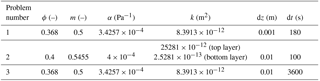
Table 1 Soil properties and discretization used in the three test problems described in Sect. 2.3.

2.3 VSFM single-column evaluation

We tested the VSFM with three idealized 1-dimensional test problems. First, the widely studied problem for the 1-D Richards equation of infiltration in dry soil by Celia et al. (1990) was used. The problem setup consists of a 1.0 m long soil column with a uniform initial pressure of −10.0 m (=3535.5 Pa). The time invariant boundary conditions applied at the top and bottom of the soil column are −0.75 m (=93989.1 Pa) and −10.0 m (=3535.5 Pa), respectively. The soil properties for this test are given in Table 1. A vertical discretization of 0.01 m is used in this simulation.

Second, we simulated transient one-dimensional vertical infiltration in a two-layered soil system as described in Srivastava and Yeh (1991). The domain consisted of a 2 m tall soil column divided equally into two soil types. Except for soil intrinsic permeability, all other soil properties of the two soil types are the same. The bottom soil is 10 times less permeable than the top (Table 1). Unlike Srivastava and Yeh (1991), who used exponential functions of soil liquid pressure to compute hydraulic conductivity and soil saturation, we used Mualem (1976) and van Genuchten (1980) constitutive relationships. Since our choice of constitutive relationships for this setup resulted in absence of an analytical solution, we compared VSFM simulations against PFLOTRAN results. The domain was discretized in 200 control volumes of equal soil thickness. Two scenarios, wetting and drying, were modeled to test the robustness of the VSFM solver robustness. Initial conditions for each scenario included a time invariant boundary condition of 0 m ($=\mathrm{1.01325}\times {\mathrm{10}}^{\mathrm{5}}$ Pa) for the lowest control volume and a constant flux of 0.9 and 0.1 cm h⁻¹ at the soil surface for wetting and drying scenarios, respectively.

Third, we compare VSFM and PFLOTRAN predictions for soil under variably saturated conditions. The 1-dimensional 1 m deep soil column was discretized in 100 equal thickness control volumes. A hydrostatic initial condition was applied such that the water table is 0.5 m below the soil surface. A time invariant flux of $\mathrm{2.5}\times {\mathrm{10}}^{-\mathrm{5}}$ m s⁻¹ is applied at the surface, while the lowest control volume has a boundary condition corresponding to the initial pressure value at the lowest soil layer. The soil properties used in this test are the same as those used in the first evaluation.

2.4 Global simulations and groundwater depth analysis

We performed global simulations with ELMv1-VSFM at a spatial resolution of 1.9^∘ (latitude) × 2.5^∘ (longitude) with a 30 (min) time step for 200 years, including a 180-year spin-up and the last 20 years for analysis. The simulations were driven by CRUNCEP meteorological forcing from 1991 to 2010 (Piao et al., 2012) and configured to use prescribed satellite phenology.

For evaluation and calibration, we used the Fan et al. (2013) global ∼1 km horizontal resolution WTD dataset (hereafter F2013 dataset), which is based on a combination of observations and hydrologic modeling. We aggregated the dataset to the ELMv1-VSFM spatial resolution. ELM-VSFM's default vertical soil discretization uses 15 soil layers to a depth of ∼42 m, with an exponentially varying soil thickness. However, ∼13 % of F2013 land grid cells have a water table deeper than 42 m. We therefore modified ELMv1-VSFM to extend the soil column to a depth of 150 m with 59 soil layers; the first nine soil layer thicknesses were the same as described in Oleson et al. (2013) and the remaining layers (10–59) were set to a thickness of 3 m.

2.5 Estimation of the subsurface drainage parameterization

In the VSFM formulation, the dominant control on long-term ground water depth is the subsurface drainage flux, q_d (kg m⁻² s⁻¹), which is calculated based on water table depth, z_∇ (m), Niu et al. (2005):

$$\begin{array}{}\text{(20)}& {\displaystyle }{q}_{\mathrm{d}}=q_{\mathrm{d},\max }\text{exp}\left(-f_{\mathrm{d}}{z}_{\mathrm{\nabla }}\right),\end{array}$$

where q_d,max (kg m⁻² s⁻¹) is the maximum drainage flux that depends on grid cell slope and f_d (m⁻¹) is an empirically derived parameter. The subsurface drainage flux formulation of Niu et al. (2005) is similar to the TOPMODEL formulation (Beven and Kirkby, 1979) and assumes the water table is parallel to the soil surface. While Sivapalan et al. (1987) derived q_d,max as a function of lateral hydraulic anisotropy, hydraulic conductivity, topographic index, and decay factor controlling vertical saturated hydraulic conductivity, Niu et al. (2005) defined q_d,max as a single calibration parameter. ELMv0 uses f_d=2.5 m⁻¹ as a global constant and estimates maximum drainage flux when WTD is at the surface as $q_{\mathrm{d},\max }=\mathrm{10}\sin \left(\mathit{\beta }\right)$ kg m⁻² s⁻¹, where β (radians) is the mean grid cell topographic slope. Of the two parameters, f_d and q_d,max, available for model calibration, we choose to calibrate f_d because the uncertainty analysis by Hou et al. (2012) identified it as the most significant hydrologic parameter in CLM4. To improve on the f_d parameter values, we performed an ensemble of global simulations with f_d values of 0.1, 0.2, 0.5, 1.0, 2.5, 5.0, 10.0, and 20 m⁻¹. Each ensemble simulation was run for 200 years to ensure an equilibrium solution, and the last 20 years were used for analysis. A nonlinear functional relationship between f_d and “WTD” was developed for each grid cell and then the F2013 dataset was used to estimate an optimal f_d for each grid cell.

2.6 Global ELM-VSFM evaluation

With the optimal f_d values, we ran a ELM-VSFM simulation using the protocol described above. We then used the ILAMB package to evaluate the ELMv1-VSFM predictions of surface energy budget, terrestrial water storage anomalies (TWSAs), and river discharge (Collier et al., 2018; Hoffman et al., 2017). ILAMB evaluates model prediction bias, RMSE, and seasonal and diurnal phasing against multiple observations of energy, water, and carbon cycles at in-situ, regional, and global scales. Since ELM-VSFM simulations in this study did not include an active carbon cycle, we used the following ILAMB benchmarks for water and energy cycles: (i) latent and surface energy fluxes using site-level measurements from FLUXNET (Lasslop et al., 2010) and globally from FLUXNET-MTE (Jung et al., 2009); (ii) TWSA from the Gravity Recovery And Climate Experiment (GRACE) observations (Kim et al., 2009); and (iii) stream flow for the 50 largest global river basins (Dai and Trenberth, 2002). We applied ILAMB benchmarks for ELMv1-VSFM simulations with default and calibrated f_d to ensure improvements in WTD predictions did not degrade model skill for other processes.

Figure 1 Comparison of VSFM simulated pressure profile (blue line) against data (red square) reported in Celia et al. (1990) at time = 24 h for infiltration in a dry soil column; Initial pressure condition is shown by green line.

3 Results and discussion

3.1 VSFM single-column evaluation

For the 1D Richards equation infiltration in dry soil comparison, we evaluated the solutions at 24 h against those published by Celia et al. (1990; Fig. 1). The VSFM solver accurately represented the sharp wetting front over time, where soil hydraulic properties change dramatically due to nonlinearity in the soil water retention curve.

For the model evaluation of infiltration and drying in layered soil, the results of the VSFM and PFLOTRAN are essentially identical. In both models and scenarios, the higher permeability top soil responds rapidly to changes in the top boundary condition and the wetting and drying fronts progressively travel through the less permeable soil layer until soil liquid pressure in the entire column reaches a new steady state by about 100 h (Fig. 2).

Figure 2 Transient liquid pressure simulated for a two-layer soil system by VSFM (solid line) and PFLOTRAN (square) for (a) wetting and (b) drying scenarios.

We also evaluated the VSFM predicted water table dynamics against PFLOTRAN predictions from an initial condition of saturated soil below 0.5 m depth. The simulated water table rises to 0.3 m depth by 1 day and reaches the surface by 2 days, and the VSFM and PFLOTRAN predictions are essentially identical (Fig. 3). Soil properties, spatial discretization, and time step used for the three single-column problems are summarized in Table 1 These three evaluation simulations demonstrate the VSFM accurately represents soil moisture dynamics under conditions relevant to ESM-scale prediction.

Figure 3 Transient (a) liquid pressure and (b) soil saturation simulated by VSFM (solid line) and PFLOTRAN (square) for the water table dynamics test problem.

3.2 Subsurface drainage parameterization estimation

The simulated nonlinear WTD–f_d relationship is a result of the subsurface drainage parameterization flux given by Eq. (20; Fig. 4a and b). For $\mathrm{0.1}\le f_{\mathrm{d}}\le \mathrm{1}$, the slope of the WTD–f_d relationship for all grid cells is log–log linear with a slope of $-\mathrm{1.0}\pm \mathrm{0.1}$. The log–log linear relationship breaks down for f_d>1, where the drainage flux becomes much smaller than infiltration and evapotranspiration (Fig. 4c and d). Thus, at larger f_d, the steady state z_∇ becomes independent of f_d and is determined by the balance of infiltration and evapotranspiration.

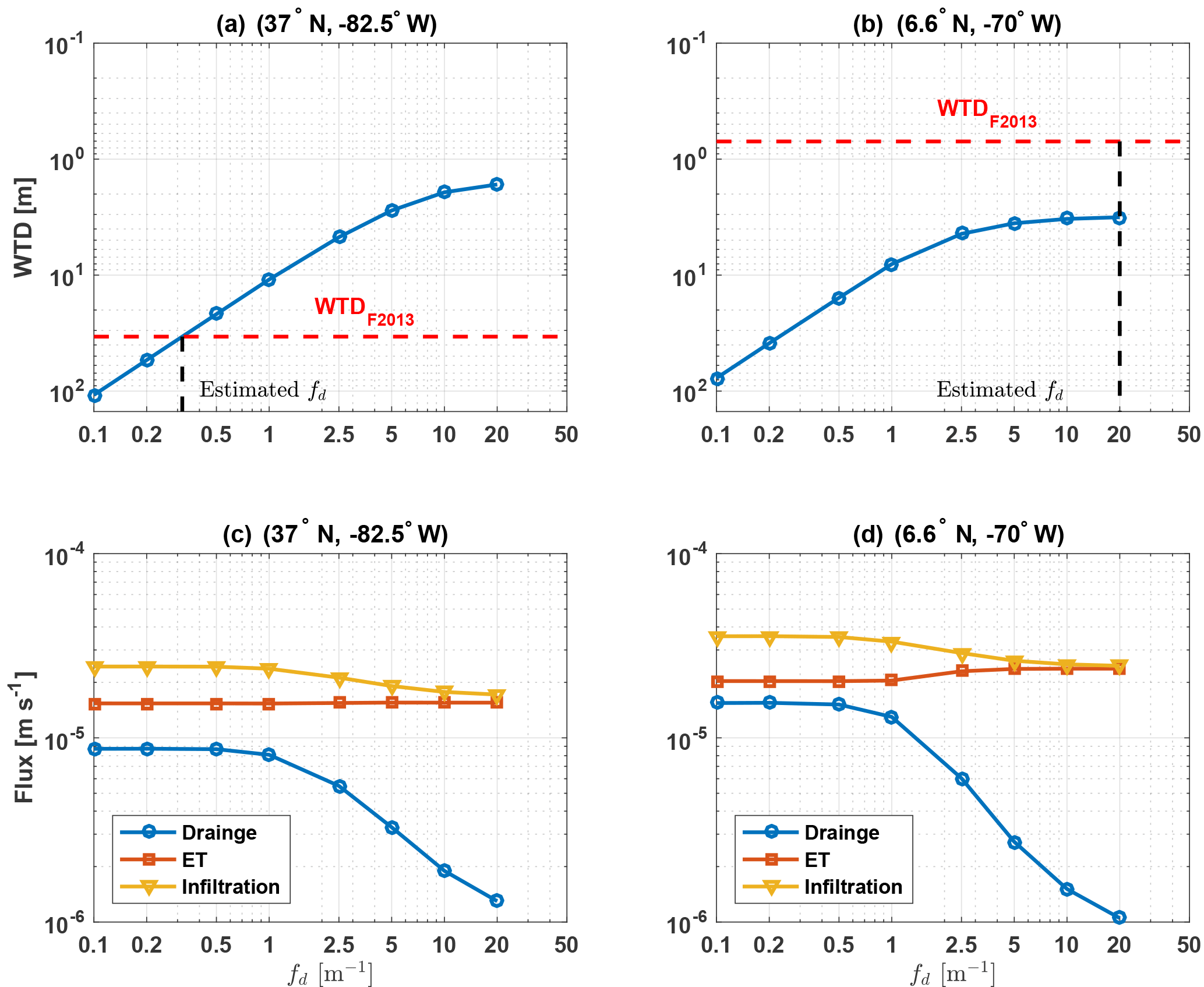
Figure 4 (a–b) The nonlinear relationship between simulated water table depth (WTD) and f_d for two grid cells within ELM's global grid. WTD from the Fan et al. (2013) dataset and optimal f_d for the two grid cells are shown with dashed red and dashed black lines, respectively. (c–d) The simulated drainage, evapotranspiration, and infiltration fluxes as functions of optimal f_d for the two ELM grid cells.

Figure 5 Global estimate of f_d.

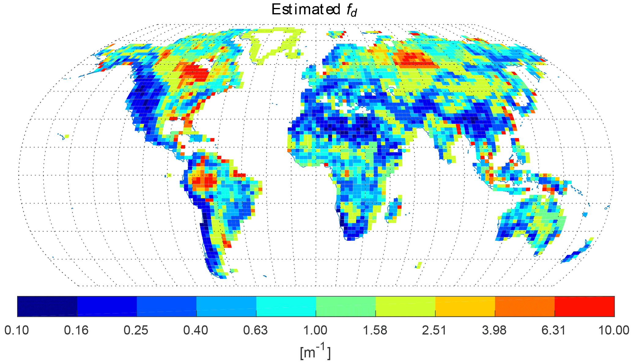
For 79 % of the global grid cells, the ensemble range of simulated WTD spanned the F2013 dataset. The optimal value of f_d for each of these grid cells was obtained by linear interpolation in the log–log space (e.g., Fig. 4a). For the remaining 21 % of grid cells where the shallowest simulated WTD across the range of f_d was deeper than that in the F2013 dataset, the optimal f_d value was chosen as the one that resulted in the lowest absolute WTD error (e.g., Fig. 4b). At large f_d values, the drainage flux has negligible effects on WTD, yet simulated WTD is not sufficiently shallow to match the F2013 observations, which indicates that either evapotranspiration is too large or infiltration is too small. There was no difference in the mean percentage of sand and clay content between grids cells with and without an optimal f_d value. The optimal f_d has a global average of 1.60 m${}^{-\mathrm{1}}\pm \mathrm{2.68}$ m⁻¹ and 72 % of global grid cells have an optimal f_d value lower than the global average (Fig. 5).

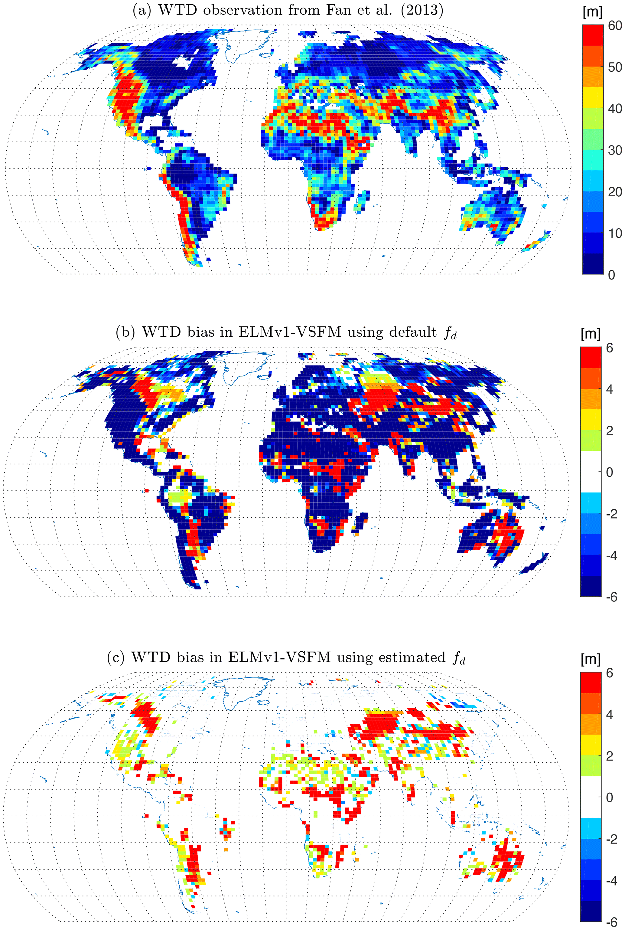
Figure 6 (a) Water table depth observation from Fan et al. (2013); (b) water table depth biases (= Model–Obs) from ELMv1-VSFM using default spatially homogeneous f_d; and (c) water table depth biases from ELMv1-VSFM using spatially heterogeneous f_d.

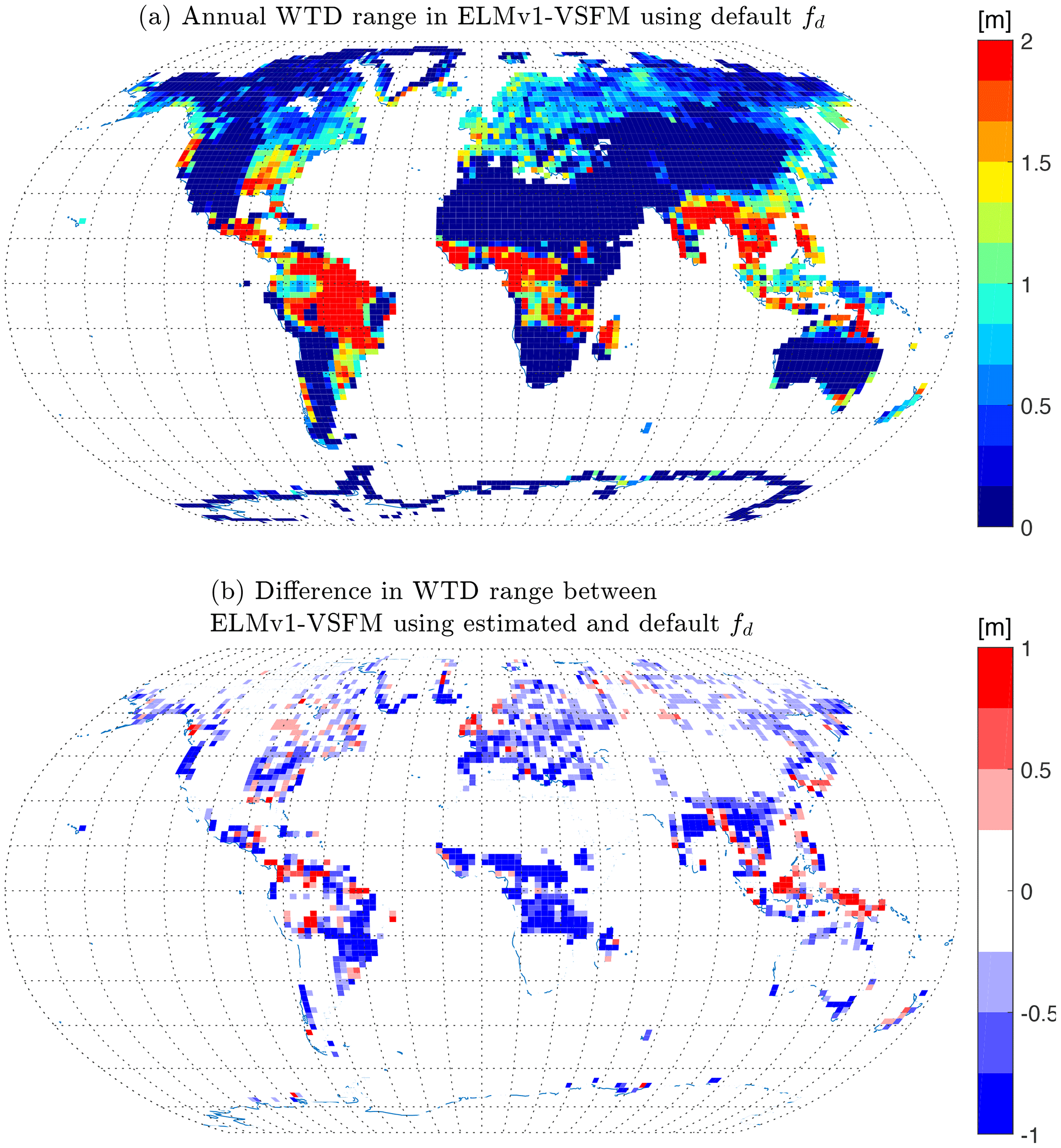
Figure 7 (a) Annual range of water table depth for ELMv1-VSFM simulation with spatially heterogeneous estimates of f_d and (b) difference in annual water table depth range between simulations with optimal and default f_d.

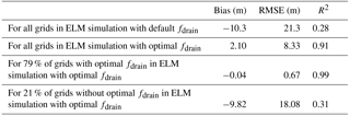
Table 2 Bias, root mean square error (RMSE), and correlation (R²) between simulated water table depth and Fan et al. (2013) data.

3.3 Global simulation evaluation

The ELMv1-VSFM predictions are much closer to the F2013 dataset (Fig. 6a) using optimal globally distributed f_d values (Fig. 6c) compared to the default f_d value (Fig. 6b). The significant reduction in WTD bias (model – observation) is mostly due to improvement in the model's ability to accurately predict deep WTD using optimal f_d values. In the simulation using optimal globally distributed f_d values, all grid cells with WTD bias >3.7 m were those for which an optimal f_d was not found. The mean global bias, RMSE, and R² values improved in the new ELMv1-VSFM compared to the default model (Table 2). The 79 % of global grid cells for which an optimal f_d value was estimated had significantly better water table prediction with a bias, RMSE, and R² of −0.04, 0.67, and 0.99 m, respectively, as compared to the remaining 21 % of global grid cells that had a bias, RMSE, and R² of −9.82, 18.08, and 0.31 m, respectively. The simulated annual WTD range, which we define to be the difference between maximum and minimum WTD in 1 year, has a spatial mean and standard deviation of 0.32 and 0.58 m, respectively, using optimal f_d values (Fig. 7a). The annual WTD range decreased by 0.24 m for the 79 % of the grid cells for which an optimal f_d value was estimated (Fig. 7b).

Globally averaged WTD in ELMv1-VSFM simulations with default f_d and optimal f_d values were 10.5 and 20.1 m, respectively. Accurate prediction of deep WTD in the simulation with optimal f_d caused very small differences in near-surface soil moisture (Fig. 8). The 79 % of grid cells with an optimal f_d value had deeper globally averaged WTDs than when using the default f_d value (24.3 vs. 8.6 m). For these 79 % of grid cells, the WTD was originally deep enough to not impact near-surface conditions (Kollet and Maxwell, 2008); therefore, further lowering of WTD led to negligible changes in near-surface hydrological conditions.

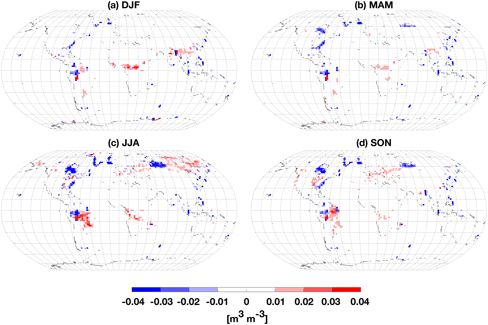
Figure 8 Seasonal monthly mean soil moisture differences for top 10 cm between ELMv1-VSFM simulations with optimal and default f_d values.

Table 3 ILAMB benchmark scores for latent heat flux (LH), sensible heat flux 640 (SH), terrestrial water storage anomaly (TWSA), and surface runoff. The calculation of ILAMB metrics and scores are described at http://redwood.ess.uci.edu/ (last access: 4 October 2018).

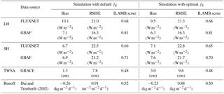
The ILAMB package (Hoffman et al., 2017) provides a comprehensive evaluation of predictions of carbon cycle states and fluxes, hydrology, surface energy budgets, and functional relationships by comparison to a wide range of observations. We used ILAMB to evaluate the hydrologic and surface energy budget predictions from the new ELMv1-VSFM model (Table 3). Optimal f_d values had inconsequential impacts on simulated surface energy fluxes at site-level and global scales. Optimal f_d values led to improvement in prediction of deep WTD (with a mean value of 24.3 m) for grid cells that had an average WTD of 8.7 m in the simulation using default f_d values. Thus, negligible differences in surface energy fluxes between the two simulations are consistent with the findings of Kollet and Maxwell (2008), who identified decoupling of groundwater dynamics and surface processes at a WTD of ∼10 m. There were slight changes in the bias and RMSE for predicted TWSA, but the ILAMB score remained unchanged. The TWSA amplitude is lower for the simulation with optimal f_d values, consistent with the associated decrease in annual WTD range. ELM's skill in simulating runoff for the 50 largest global watersheds remained unchanged. Two additional 10-year-long simulations were performed to investigate the sensitivity of VSFM simulated WTD to spatial and temporal discretization. Results show that simulated WTD is insensitive to temporal discretization, and has small sensitivity to vertical spatial resolution. See the Supplement for details regarding the setup and analysis of results from the two additional simulations.

Finally, we evaluated the computational costs of implementing VSFM in ELM and compared them to the default model. We performed 5-year-long simulations for default and VSFM using 96, 192, 384, 768, and 1536 cores on the Edison supercomputer at the National Energy Research Scientific Computing Center. Using an optimal processor layout, we found that ELMv1-VSFM is ∼30 % more expensive than the default ELMv1 model (the Supplement, Fig. S1). We note that the relative computational cost of the land model in a fully coupled global model simulation is generally very low. Dennis et al. (2012) reported computational cost of the land model to be less than 1 % in ultrahigh-resolution CESM simulations. We therefore believe that the additional benefits associated with the VSFM formulation are well justified by this modest increase in computational cost. In particular, VSFM allows for a greater variety of mesh configurations and boundary conditions, and can accurately simulate WTD for the ∼13 % of global grid cells that have a water table deeper than 42 (m) (Fan et al., 2013).

3.4 Caveats and future work

The significant improvement in WTD prediction using optimal f_d values demonstrates VSFM's capabilities to model hydrologic processes using a unified physics formulation for unsaturated–saturated zones. However, several caveats remain due to uncertainties in model structure, model parameterizations, and climate forcing data.

In this study, we assumed a spatially homogeneous depth to bedrock (DTB) of 150 m. Recently, Brunke et al. (2016) incorporated a global ∼1 km dataset of soil thickness and sedimentary deposits (Pelletier et al., 2016) in CLM4.5 to study the impacts of soil thickness spatial heterogeneity on simulated hydrological and thermal processes. While inclusion of heterogeneous DTB in CLM4.5 added more realism to the simulation setup, no significant changes in simulated hydrologic and energy fluxes were reported by Brunke et al. (2016). Presently, work is ongoing in the E3SM project to include variable DTB within ELM and future simulations will examine the impact of those changes on VSFM's prediction of WTD. Our use of the “satellite phenology” mode, which prescribes transient leaf area index profiles for each PFT in the grid cell, ignored the likely influence of water cycle dynamics and nutrient constraints on the C cycle (Ghimire et al., 2016; Zhu et al., 2016). Estimation of soil hydraulic properties based on soil texture data is critical for accurate LSM predictions (Gutmann and Small, 2005) and this study does not account for uncertainty in soil hydraulic properties.

Lateral water redistribution impacts soil moisture dynamics (Bernhardt et al., 2012), biogeochemical processes in the root zone (Grant et al., 2015), distribution of vegetation structure (Hwang et al., 2012), and land–atmosphere interactions (Chen and Kumar, 2001; Rihani et al., 2010). The ELMv1-VSFM developed in this study does not include lateral water redistribution between soil columns and only simulates vertical water transport. Lateral subsurface processes can be included in LSMs via a range of numerical discretization approaches of varying complexity, e.g., adding lateral water as source/sink terms in the 1-D model, implementing an operator split approach to solve vertical and lateral processes in a noniterative approach (Ji et al., 2017), or solving a fully coupled 3-D model (Bisht et al., 2017, 2018; Kollet and Maxwell, 2008). Additionally, lateral transport of water can be implemented in LSMs at a subgrid level (Milly et al., 2014) or grid cell level (Miguez-Macho et al., 2007). The current implementation of VSFM is such that each processor solves the variably saturated Richards equation for all independent soil columns as one single problem. Thus, extension of VSFM to solve the tightly coupled 3-D Richards equation on each processor locally while accounting for lateral transport of water within grid cells and among grid cells is straightforward. The current VSFM implementation can also be easily extended to account for subsurface transport of water among grid cells that are distributed across multiple processors by modeling lateral flow as source/sink terms in the 1-D model. Tradeoffs between approaches to represent lateral processes and computational costs need to be carefully studied before developing quasi- or fully three-dimensional LSMs (Clark et al., 2015).

Transport of water across multiple components of the soil-plant-atmosphere continuum (SPAC) has been identified as a critical process in understanding the impact of climate warming on the global carbon cycle (McDowell and Allen, 2015). Several SPAC models have been developed by the ecohydrology community and applied to study site level processes (Amenu and Kumar, 2008; Bohrer et al., 2005; Manoli et al., 2014; Sperry et al., 1998), yet implementation of SPAC models in global LSMs is limited (Clark et al., 2015). Similarly, current generation LSMs routinely ignore advective heat transport within the subsurface, which has been shown to be important in high-latitude environments by multiple field and modeling studies (Bense et al., 2012; Frampton et al., 2011; Grant et al., 2017; Kane et al., 2001). The use of PETSc's DMComposite in VSFM provides flexibility for solving a tightly coupled multi-component problem (e.g., transport of water through the soil-plant-atmosphere continuum) and multi-physics problem (e.g., fully coupled conservation of mass and energy equations in the subsurface). DMComposite allows for an easy assembly of a tightly coupled multi-physics problem from individual physics formulations (Brown et al., 2012).

4 Summary and conclusion

Starting from the climate-scale land model ELMv0, we incorporated a unified physics formulation to represent soil moisture and groundwater dynamics that are solved using PETSc. Application of VSFM to three benchmarks problems demonstrated its robustness to simulate subsurface hydrologic processes in coupled unsaturated and saturated zones. Ensemble global simulations at 1.9^∘ × 2.5^∘ were performed for 200 years to obtain spatially heterogeneous estimates of the subsurface drainage parameter, f_d, that minimized mismatches between predicted and observed WTDs. In order to simulate the deepest water table reported in the Fan et al. (2013) dataset, we used 59 vertical soil layers that reached a depth of 150 m.

An optimal f_d was obtained for 79 % of the grids cells in the domain. For the remaining 21 % of grid cells, simulated WTD always remained deeper than observed. Calibration of f_d significantly improved global WTD prediction by reducing bias and RMSE and increasing R². Grids without an optimal f_d were the largest contributor to error in WTD predication. ILAMB benchmarks on simulations with default and optimal f_d showed negligible changes to surface energy fluxes, TWSA, and runoff. ILAMB metrics ensured that model skill was not adversely impacted for all other processes when optimal f_d values were used to improve WTD prediction.

Appendix A: Smooth approximation of Brooks–Corey water retention curve

The Brooks and Corey (1964) water retention curve of Eq. (10) has a discontinuous derivative at $P_{\mathrm{c}}=P_{\mathrm{c}}^{\mathrm{0}}$. Figure A1 illustrates an example. To improve convergence of the nonlinear solver at small capillary pressures, the smoothed Brooks–Corey function introduces a cubic polynomial, B(P_c), in the neighborhood of $P_{\mathrm{c}}^{\mathrm{0}}$.

$$\begin{array}{}\text{(A1)}& {\displaystyle }{s}_{\mathrm{e}}=\left\{\begin{array}{l}{\left(-\mathit{\alpha }{P}_{\mathrm{c}}\right)}^{-\mathit{\lambda }}\text{if}{P}_{\mathrm{c}}\le P_{\mathrm{u}},\\ B\left(P_{\mathrm{c}}\right)\text{if}{P}_{\mathrm{u}}<P_{\mathrm{c}}<P_{\mathrm{s}},\\ \mathrm{1}\text{if}{P}_{\mathrm{s}}\le P_{\mathrm{s}},\end{array}\right.\end{array}$$

where the breakpoints P_u and P_s satisfy $P_{\mathrm{u}}<P_{\mathrm{c}}^{\mathrm{0}}<P_{\mathrm{s}}\le \mathrm{0}$. The smoothing polynomial

$$\begin{array}{ll}{\displaystyle }B\left(P_{\mathrm{c}}\right)& {\displaystyle }=b_{\mathrm{0}}+b_{\mathrm{1}}\left(P_{\mathrm{c}}-P_{\mathrm{s}}\right)+b_{\mathrm{2}}{\left(P_{\mathrm{c}}-P_{\mathrm{s}}\right)}^{\mathrm{2}}\\ \text{(A2)}& {\displaystyle }& {\displaystyle }+b_{\mathrm{3}}{\left(P_{\mathrm{c}}-P_{\mathrm{s}}\right)}^{\mathrm{3}}\end{array}$$

introduces four more parameters, whose values follow from continuity. In particular, matching the saturated region requires $B\left(P_{\mathrm{s}}\right)=b_{\mathrm{0}}=\mathrm{1}$, and a continuous derivative at P_c=P_s requires $B{}^{\prime }\left(P_{\mathrm{s}}\right)=b_{\mathrm{1}}=\mathrm{0}$. Similarly, matching the value and derivative at P_c=P_u requires

$$\begin{array}{}\text{(A3)}& {\displaystyle }{b}_{\mathrm{2}}={\displaystyle \frac{-\mathrm{1}}{{\mathrm{\Delta }}^{\mathrm{2}}}}\left[\mathrm{3}-{\left(\mathit{\alpha }{P}_{\mathrm{u}}\right)}^{-\mathit{\lambda }}\left(\mathrm{3}+{\displaystyle \frac{\mathit{\lambda }\mathrm{\Delta }}{P_{\mathrm{u}}}}\right)\right],\text{(A4)}& {\displaystyle }{b}_{\mathrm{3}}={\displaystyle \frac{-\mathrm{1}}{{\mathrm{\Delta }}^{\mathrm{3}}}}\left[\mathrm{2}-{\left(\mathit{\alpha }{P}_{\mathrm{u}}\right)}^{-\mathit{\lambda }}\left(\mathrm{2}+{\displaystyle \frac{\mathit{\lambda }\mathrm{\Delta }}{P_{\mathrm{u}}}}\right)\right],\end{array}$$

where $\mathrm{\Delta }=P_{\mathrm{u}}-P_{\mathrm{s}}$. Note that $P_{\mathrm{u}}\le \mathrm{\Delta }<\mathrm{0}$.

In practice, setting P_u too close to $P_{\mathrm{c}}^{\mathrm{0}}$ can produce an unwanted local maximum in the cubic smoothing regime, resulting in s_e>1. Avoiding this condition requires that B(P_c) increase monotonically from P_c=P_u, where $B{}^{\prime }\left(P_{\mathrm{c}}\right)>\mathrm{0}$, to P_c=P_s, where $B{}^{\prime }\left(P_{\mathrm{c}}\right)=\mathrm{0}$. Thus a satisfactory pair of breakpoints ensures

$$\begin{array}{}\text{(A5)}& {\displaystyle }B{}^{\prime }\left(P_{\mathrm{c}}\right)=\left[P_{\mathrm{c}}-P_{\mathrm{s}}\right]\left[\mathrm{2}{b}_{\mathrm{2}}+\mathrm{3}{b}_{\mathrm{3}}\left(P_{\mathrm{c}}-P_{\mathrm{s}}\right)\right]>\mathrm{0}\end{array}$$

throughout $P_{\mathrm{u}}\le P_{\mathrm{c}}<P_{\mathrm{s}}$.

Figure A1 The Brooks–Corey water rendition curve for estimating liquid saturation, s_e, as a function of capillary pressure, P_c, shown in solid black line and smooth approximation of Brooks–Corey (SBC) are shown in dashed line.

Let $P_{\mathrm{c}}^{\ast }$ denote a local extremum of B, so that $B{}^{\prime }\left(P_{\mathrm{c}}^{\ast }\right)=\mathrm{0}$. If $P_{\mathrm{c}}^{\ast }\ne P_{\mathrm{s}}$, it follows $P_{\mathrm{c}}^{\ast }-P_{\mathrm{s}}=-\mathrm{2}{b}_{\mathrm{2}}/\left(\mathrm{3}{b}_{\mathrm{3}}\right)$. Rewriting Eq. (22), $B{}^{\prime }\left(P_{\mathrm{c}}\right)=\left(P_{\mathrm{c}}-P_{\mathrm{s}}\right)\mathrm{3}{b}_{\mathrm{3}}\left(P_{\mathrm{c}}-P_{\mathrm{c}}^{\ast }\right)$ shows that $B{}^{\prime }\left(P_{\mathrm{u}}\right)>\mathrm{0}$ requires either: (1) b₃<0 and $P_{\mathrm{c}}^{\ast }<P_{\mathrm{u}}$; or (2) b₃>0 and $P_{\mathrm{c}}^{\ast }>P_{\mathrm{u}}$. The first possibility places $P_{\mathrm{c}}^{\ast }$ outside the cubic smoothing regime, and so does not constrain the choice of P_u or P_s. The second possibility allows for an unwanted local extremum at $P_{\mathrm{u}}<P_{\mathrm{c}}^{\ast }<P_{\mathrm{s}}$. In this case, b₃>0 implies b₂<0 (since $P_{\mathrm{c}}^{\ast }<P_{\mathrm{s}}\le \mathrm{0})$. Then since $B{}^{\prime \prime }\left(P_{\mathrm{c}}^{\ast }\right)=-\mathrm{2}{b}_{\mathrm{2}}$, the local extremum is a maximum, resulting in $s_{\mathrm{e}}\left(P_{\mathrm{c}}^{\ast }\right)>\mathrm{1}$.

Given a breakpoint P_s, one strategy for choosing P_u is to guess a value, then check whether the resulting b₂ and b₃ produces $P_{\mathrm{u}}<P_{\mathrm{c}}^{\ast }<P_{\mathrm{s}}$. If so, P_u should be made more negative. An alternative strategy is to choose P_u in order the guarantee acceptable values for b₂ and b₃. One convenient choice forces b₂=0. Another picks P_u in order to force b₃=0. Both of these reductions (1) ensure B(P_c) has a positive slope throughout the smoothing interval, (2) slightly reduce the computation cost of finding s_e(P_c) for P_c on the smoothing interval, and (3) significantly reduce the computational cost of inverting the model, in order to find P_c as a function of s_e.

As shown in Fig. A1, the two reductions differ mainly in that setting b₂=0 seems to produce narrower smoothing regions (probably due to the fact that this choice gives zero curvature at P_c=P_s, while b₃=0 yields a negative second derivative there). However, we have not verified this observation analytically.

Both reductions require solving a nonlinear expression, either Eqs. (A3) or (A4), for P_u. While details are beyond the scope of this paper, we note that we have used a bracketed Newton–Raphson method. The search switches to bisection when Newton–Raphson would jump outside the bounds established by previous iterations, and by the requirement $P_{\mathrm{u}}<P_{\mathrm{c}}^{\mathrm{0}}$. In any event, since the result of this calculation may be cached for use throughout the simulation, it need not be particularly efficient.

Appendix B: Residual equation of VSFM formulation

The residual equation for the VSFM formulation at t+1 time level for nth control volume is given by

$$\begin{array}{ll}{\displaystyle }{R}_n^{t+\mathrm{1}}& {\displaystyle }\equiv \left({\displaystyle \frac{{\left(\mathit{\varphi }{s}_{\mathrm{w}}\mathit{\rho }\right)}_n^{t+\mathrm{1}}-{\left(\mathit{\varphi }{s}_{\mathrm{w}}\mathit{\rho }\right)}_n^t}{\mathrm{\Delta }t}}\right)V_n+\sum _{n^{\prime }}{\left(\mathit{\rho }\mathbf{q}\right)}_{n{n}^{\prime }}^{t+\mathrm{1}}\\ \text{(B1)}& {\displaystyle }& {\displaystyle }\cdot A_{nn{}^{\prime }}+Q_n^{t+\mathrm{1}}{V}_n=\mathrm{0},\end{array}$$

where ϕ (mm³ mm³) is the soil porosity, s_w (-) is saturation, ρ (kg m⁻³) is water density, ${}_{nn{}^{\prime }}$ (m s⁻¹) is the Darcy flow velocity between nth and n^′th control volumes, $A_{nn{}^{\prime }}$ (m s⁻¹) is the interface area between nth and n^′th control volumes, and Q (kg m⁻³ s⁻¹) is a sink of water. The Darcy velocity is computed as

$$\begin{array}{}\text{(B2)}& {\displaystyle }{\mathbf{q}}_{nn{}^{\prime }}=-{\left({\displaystyle \frac{k{k}_r}{\mathit{\mu }}}\right)}_{nn{}^{\prime }}\left[{\displaystyle \frac{P_{n{}^{\prime }}-P_n-{\mathit{\rho }}_{nn{}^{\prime }}(\mathbf{g}\cdot {\mathbf{d}}_{nn{}^{\prime }})}{d_n+d_{n{}^{\prime }}}}\right]{\mathbf{n}}_{nn{}^{\prime }},\end{array}$$

where κ (m⁻²) is intrinsic permeability, κ_r (-) is relative permeability, μ (Pa s) is viscosity of water, P (Pa) is pressure, g (m s⁻²) is the acceleration due to gravity, d_n (m) and $d_{n{}^{\prime }}$ (m) are the distances between centroid of the nth and n^′th control volume to the common interface between the two control volumes, ${\mathbf{d}}_{nn{}^{\prime }}$ is a distance vector joining centroid of nth and n^′th control volume, and ${\mathbf{n}}_{nn{}^{\prime }}$ is a unit normal vector joining centroid of the nth and n^′th control volume.

The density at the interface of control volume, ${\mathit{\rho }}_{nn{}^{\prime }}$, is computed as the inverse distance weighted average by

$$\begin{array}{}\text{(B3)}& {\displaystyle }{\mathit{\rho }}_{nn{}^{\prime }}={\mathit{\omega }}_{n{}^{\prime }}{\mathit{\rho }}_n+{\mathit{\omega }}_n{\mathit{\rho }}_{n{}^{\prime }},\end{array}$$

where ω_n and ${\mathit{\omega }}_{n{}^{\prime }}$ are given by

$$\begin{array}{}\text{(B4)}& {\displaystyle }{\mathit{\omega }}_n={\displaystyle \frac{d_n}{d_n+d_{n{}^{\prime }}}}=(\mathrm{1}-{\mathit{\omega }}_{n{}^{\prime }}).\end{array}$$

The first term on the right-hand side of Eq. (27) is computed as the product of distance-weighted harmonic average of intrinsic permeability, $k_{nn{}^{\prime }}$, and upwinding of $k_r/\mathit{\mu }(=\mathit{\lambda })$ as

$$\begin{array}{}\text{(B5)}& {\displaystyle }{\left({\displaystyle \frac{k{k}_r}{\mathit{\mu }}}\right)}_{nn{}^{\prime }}=k_{nn{}^{\prime }}{\left({\displaystyle \frac{k_r}{\mathit{\mu }}}\right)}_{nn{}^{\prime }}=\left[{\displaystyle \frac{k_n{k}_{n{}^{\prime }}(d_n+d_{n{}^{\prime }})}{k_n{d}_{n{}^{\prime }}+k_{n{}^{\prime }}{d}_n)}}\right]{\mathit{\lambda }}_{nn{}^{\prime }},\end{array}$$

where

$$\begin{array}{}\text{(B6)}& {\displaystyle }{\mathit{\lambda }}_{nn{}^{\prime }}=\left\{\begin{array}{l}{\left(k_{\mathrm{r}}/\mathit{\mu }\right)}_n\text{if}{\mathit{q}}_{nn{}^{\prime }}>\mathrm{0},\\ {\left(k_{\mathrm{r}}/\mathit{\mu }\right)}_{n{}^{\prime }}\text{otherwise}.\end{array}\right.\end{array}$$

By substituting Eqs. (28), (29), and (30) in Eq. (27), we obtain

$$\begin{array}{ll}{\displaystyle }& {\displaystyle }{\mathbf{q}}_{nn{}^{\prime }}=-\left[{\displaystyle \frac{k_n{k}_{n{}^{\prime }}}{k_n{d}_{n{}^{\prime }}+k_{n{}^{\prime }}{d}_n)}}\right]{\mathit{\lambda }}_{nn{}^{\prime }}\\ \text{(B7)}& {\displaystyle }& {\displaystyle }[P_{n{}^{\prime }}-P_n-{\mathit{\rho }}_{nn{}^{\prime }}({\mathbf{gd}}_{nn{}^{\prime }}\left)\right]{\mathbf{n}}_{nn{}^{\prime }}.\end{array}$$

Appendix C: Jacobian equation of VSFM formulation

The discretized equations of VSFM leads to a system of nonlinear equations given by ${\mathbf{R}}^{t+\mathrm{1}}\left({\mathbf{P}}^{t+\mathrm{1}}\right)=\mathrm{0}$, which are solved using Newton's method using the Portable, Extensible Toolkit for Scientific Computing (PETSc) library. The algorithm of Newton's method requires solution of the following linear problem

$$\begin{array}{}\text{(C1)}& {\displaystyle }{\mathbf{J}}^{t+\mathrm{1},k}\left({\mathbf{P}}^{t+\mathrm{1},k}\right)\mathrm{\Delta }{\mathbf{P}}^{t+\mathrm{1},k}=-{\mathbf{R}}^{t+\mathrm{1},k}\left({\mathbf{P}}^{t+\mathrm{1},k}\right),\end{array}$$

where ${\mathbf{J}}^{t+\mathrm{1},k}\left({\mathbf{P}}^{t+\mathrm{1},k}\right)$ is the Jacobian matrix. In VSFM, the Jacobian matrix is computed analytically. The contribution to the diagonal and off-diagonal entry of the Jacobian matrix from nth residual equations are given by

$$\begin{array}{ll}{\displaystyle }{J}_{nn}& {\displaystyle }={\displaystyle \frac{\partial R_n}{\partial P_n}}=\left({\displaystyle \frac{V_n}{\mathrm{\Delta }t}}\right){\displaystyle \frac{\partial \left(\mathit{\rho }\mathit{\varphi }{s}_{\mathrm{w}}\right)}{\partial P_n}}+\sum _{n^{\prime }}{\displaystyle \frac{\partial (\mathit{\rho }\mathbf{q}{)}_{nn{}^{\prime }}}{\partial P_n}}{A}_{nn{}^{\prime }}\\ \text{(C2)}& {\displaystyle }& {\displaystyle }+{\displaystyle \frac{\partial Q_n^{t+\mathrm{1}}}{\partial P_n}}{V}_n,{\displaystyle }{J}_{nn{}^{\prime }}& {\displaystyle }={\displaystyle \frac{\partial R_n}{\partial P_{n{}^{\prime }}}}=\sum _{n^{\prime }}{\displaystyle \frac{\partial (\mathit{\rho }\mathbf{q}{)}_{nn{}^{\prime }}}{\partial P_{n{}^{\prime }}}}{\mathbf{A}}_{nn{}^{\prime }}\\ \text{(C3)}& {\displaystyle }& {\displaystyle }+{\displaystyle \frac{\partial Q_n^{t+\mathrm{1}}}{\partial P_{n{}^{\prime }}}}{V}_n.\end{array}$$

The derivative of the accumulation term in J_nn is computed as

$$\begin{array}{}\text{(C4)}& {\displaystyle \frac{\partial \left(\mathit{\rho }\mathit{\varphi }{s}_{\mathrm{w}}\right)}{\partial P_n}}=\mathit{\varphi }{s}_{\mathrm{w}}{\displaystyle \frac{\partial \mathit{\rho }}{\partial P_n}}+\mathit{\rho }{s}_{\mathrm{w}}{\displaystyle \frac{\partial \mathit{\varphi }}{\partial P_n}}+\mathit{\rho }\mathit{\varphi }{\displaystyle \frac{\partial s_{\mathrm{w}}}{\partial P_n}}.\end{array}$$

The derivative of flux between nth and n^′th control volume with respect to pressure of each control volume is given as

$$\begin{array}{}\text{(C5)}& {\displaystyle \frac{\partial (\mathit{\rho }\mathbf{q}{)}_{nn{}^{\prime }}}{\partial P_n}}={\mathit{\rho }}_{nn{}^{\prime }}{\displaystyle \frac{\partial {\mathbf{q}}_{nn{}^{\prime }}}{\partial P_n}}+{\mathbf{q}}_{nn{}^{\prime }}{\mathit{\omega }}_n{\displaystyle \frac{\partial {\mathit{\rho }}_n}{\partial P_n}},\text{(C6)}& {\displaystyle \frac{\partial (\mathit{\rho }\mathbf{q}{)}_{nn{}^{\prime }}}{\partial P_{n{}^{\prime }}}}={\mathit{\rho }}_{nn{}^{\prime }}{\displaystyle \frac{\partial {\mathbf{q}}_{nn{}^{\prime }}}{\partial P_{n{}^{\prime }}}}+{\mathbf{q}}_{nn{}^{\prime }}{\mathit{\omega }}_{n{}^{\prime }}{\displaystyle \frac{\partial {\mathit{\rho }}_{n{}^{\prime }}}{\partial P_{n{}^{\prime }}}}.\end{array}$$

Lastly, the derivative of the Darcy velocity between the nth and n^′th control volume with respect to pressure of each control volume is given as

$$\begin{array}{ll}{\displaystyle \frac{\partial {\mathbf{q}}_{nn{}^{\prime }}}{\partial P_n}}=& {\displaystyle }\left[{\displaystyle \frac{k_n{k}_{n{}^{\prime }}}{k_n{d}_{n{}^{\prime }}+k_{n{}^{\prime }}{d}_n)}}\right]{\mathit{\lambda }}_{nn{}^{\prime }}\left[\mathrm{1}+{\mathit{\omega }}_n\left(\mathbf{g}.{\mathbf{d}}_{nn{}^{\prime }}\right){\displaystyle \frac{\partial {\mathit{\rho }}_n}{\partial P_n}}\right]\\ \text{(C7)}& {\displaystyle }& {\displaystyle }{\mathbf{n}}_{nn{}^{\prime }}+{\mathbf{q}}_{nn{}^{\prime }}{\displaystyle \frac{\partial \left(ln\left({\mathit{\lambda }}_{nn{}^{\prime }}\right)\right)}{\partial P_n}},{\displaystyle \frac{\partial {\mathbf{q}}_{nn{}^{\prime }}}{\partial P_{n{}^{\prime }}}}=& {\displaystyle }\left[{\displaystyle \frac{k_n{k}_{n{}^{\prime }}}{k_n{d}_{n{}^{\prime }}+k_{n{}^{\prime }}{d}_n)}}\right]{\mathit{\lambda }}_{nn{}^{\prime }}\left[-\mathrm{1}+{\mathit{\omega }}_n\left(\mathbf{g}.{\mathbf{d}}_{nn{}^{\prime }}\right){\displaystyle \frac{\partial {\mathit{\rho }}_{n{}^{\prime }}}{\partial P_{n{}^{\prime }}}}\right]\\ \text{(C8)}& {\displaystyle }& {\displaystyle }{\mathbf{n}}_{nn{}^{\prime }}+{\mathbf{q}}_{nn{}^{\prime }}{\displaystyle \frac{\partial \left(ln\left({\mathit{\lambda }}_{nn{}^{\prime }}\right)\right)}{\partial P_{n{}^{\prime }}}}.\end{array}$$

Appendix D: Numerical checks in VSFM

VSFM uses a two-stage check to determine an acceptable numerical solution

• Stage-1: at any temporal integration stage, the model attempts to solve the set of nonlinear equations given by Eq. (19) with a given time step. If the model fails to find a solution to the nonlinear equations with a given error tolerance settings, the time step is reduced by half and the model again attempts to solve the nonlinear problem. If the model fails to find a solution after a maximum number of time step cuts (currently 20), the model reports an error and stops execution. None of the simulations reported in this paper failed this check.

• Stage-2: after a numerical solution for the nonlinear problem is obtained, a mass balance error is calculated as the difference between input and output fluxes and change in mass over the integration time step. If the mass balance error exceeds 10–5 kg m⁻², the error tolerances for the nonlinear problem are tightened by a factor of 10 and the model re-enters Stage-1. If the model fails to find a solution with an acceptable mass balance error after 10 attempts of tightening error tolerances, the model reports an error and stops execution. None of the simulations reported in this paper failed this check.