the Creative Commons Attribution 4.0 License.
the Creative Commons Attribution 4.0 License.
 | 03 Sep 2018
FAME (v1.0): a simple module to simulate the effect of planktonic foraminifer species-specific habitat on their oxygen isotopic content
Didier M. Roche
Claire Waelbroeck
Brett Metcalfe
Thibaut Caley
The oxygen-18 to oxygen-16 ratio recorded in fossil planktonic foraminifer shells has been used for over 50 years in many geoscience applications. However, different planktonic foraminifer species generally yield distinct signals, as a consequence of their specific living habitats in the water column and along the year. This complexity is usually not taken into account in model–data integration studies. To overcome this shortcoming, we developed the Foraminifers As Modeled Entities (FAME) module. The module predicts the presence or absence of commonly used planktonic foraminifers and their oxygen-18 values. It is only forced by hydrographic data and uses a very limited number of parameters, almost all derived from culture experiments. FAME performance is evaluated using the Multiproxy Approach for the Reconstruction of the Glacial Ocean surface (MARGO) Late Holocene planktonic foraminifer calcite oxygen-18 and abundance datasets. The application of FAME to a simple cooling scenario demonstrates its utility to predict changes in planktonic foraminifer oxygen-18 to oxygen-16 ratio in response to changing climatic conditions.
- Article
(4717 KB) - Full-text XML
-
Supplement
(61 KB) - BibTeX
- EndNote


Since the early work of Emiliani (1955), oxygen-18 isotopic abundance in calcite fossil foraminifer tests recovered from oceanic sediments has been widely used to reconstruct the past variations in oxygen-18 content of seawater as well as its temperature, the two main variables that affect the ratios of oxygen-18 to oxygen-16 in calcite (hereafter R18Oc). The recognition that different species of foraminifers from the same sediment core yielded different R18Oc was made early on (e.g., Duplessy et al., 1970; Lidz et al., 1968; Berger, 1969; Fairbanks and Wiebe, 1980; Deuser, 1987), though it was an attempt by Emiliani (1954) to relate depth habitat of foraminifers to the density of seawater that led to the revelation that the R18Oc recorded by fossil foraminifers likely reflected the average depth habitat of individual species. Through in situ water column sampling via opening–closing plankton nets, Jones (1967) through faunal abundance counts corroborated the depth habitats that Emiliani (1954) inferred through isotopic analysis. However, increased plankton sampling (Bé and Tolderlund, 1971) and the advent of the sediment trap have shown that different species have different living habitats in the water column and throughout the year and that in some cases the foraminiferal R18Oc presents an offset with respect to the equilibrium calcite oxygen-18 to oxygen-18 ratio (Mix, 1987; Bijma and Hemleben, 1994; Ortiz et al., 1995; Kohfeld et al., 1996; Bauch et al., 1997; Schiebel et al., 2002; Simstich et al., 2003; Mortyn and Charles, 2003; Rebotim et al., 2017; Jonkers and Kucera, 2015). This complexity is usually not accounted for in paleoceanographic studies. Instead, the approximation is often made that each planktonic foraminifer species has an apparent living depth – defined as the water depth where equilibrium calcite formation would approximate their measured calcite R18Oc value in the water column – that can vary by hundreds of meters from one region to another. To correctly interpret the wealth of information coming from the calcite oxygen-18 to oxygen-16 ratio record, especially when multiple species are measured at the same geographical location, there is a need to take into account the impact of depth habitat and growth season on each species' calcite oxygen-18. Minor contributors to the resultant calcite R18Oc, such as carbonate ion concentration (Spero et al., 1997; Pearson, 2012) and symbionts (e.g., Ezard et al., 2015; Spero, 1998), may modulate the absolute values, making species-specific comparisons problematic; however, their overall contribution may also covary and/or autocorrelate with temperature and latitudinal gradients; therefore, this paper focuses on the major components only.
In recent years, the development of water-isotope-enabled ocean models has allowed the simulation of the two variables at the root of the calcite R18Oc record: seawater temperature and oxygen-18 abundance. So far, water-isotope-based model–data studies have generally compared planktonic oxygen-18 ratios to equilibrium calcite R18Oc values. The equilibrium calcite ratio in that case is computed from annual averaged seawater temperatures and oxygen-18 abundance taken either at surface or averaged over the upper 50 to 100 m of the water column (e.g., Caley et al., 2014; Werner et al., 2016). To go one step further, it is necessary to account for species-specific habitat when computing calcite R18Oc. The Foraminifers As Modeled Entities (FAME) approach is underpinned by two arguably simple principles: (1) the weighting due to species habitat is reflected in the calcite oxygen-18 ratio record, and (2) the model derived should be kept simple to allow its offline application to the output of climatic models without the need of rerunning the entire climate model simulations.
After having developed the FAME methodology, we found out that the idea was already present in a theoretical framework in Mix (1987) and in one following study (Mulitza et al., 1997), in the latter referred to as Mix's model. The most notable difference between the early study of Mix (1987) and the present one is the actual definition of the weighting functions. Mix (1987) assumed them to be simple Gaussians, whereas we build ours on the laboratory culture-based equations of planktonic foraminifer growth rates as a function of temperature given in Lombard et al. (2009).
Since the early work of Mix (1987), other methods were developed to approach the species-specific complexity of planktonic foraminifers. Schmidt (1999) developed a simple module to compute planktonic foraminifer R18Oc in a water-isotope-enabled global ocean model. However, in his approach, water depths at which planktonic foraminifers calcify and their seasonal growth patterns are fixed for each species. Therefore, such a module cannot properly account for the impact of climatic changes on foraminifer living conditions. Fraile et al. (2008) and Lombard et al. (2011) developed models predicting the abundance of common planktonic foraminifer species in response to hydrographic data and food concentration. Both these models predict the relative abundances of the different simulated foraminifer species, an information which is not needed to assess individual species' oxygen-18 but entails a large number of empirical parameters, i.e., 21 and 15 parameters per planktonic foraminifer species in Fraile et al. (2008) and Lombard et al. (2011), respectively. Moreover, Fraile et al. (2008) derived the sensitivity of each species with respect to temperature from sediment-trap data, so that their model can only account for changes in seasonality and not in depth habitat. In contrast, the FORAMCLIM model (Lombard et al., 2011) predicts both season and water depth of each species' potential maximum abundance. In fact, FAME can be viewed as a simplified version of FORAMCLIM (only retaining FORAMCLIM computation of growth rates as a function of temperature), expanded by a mechanistic calculation of species-dependent calcite oxygen-18. FAME is only forced by hydrographic data and only uses six parameters per planktonic foraminifer species that are all derived from culture experiments, plus one parameter accounting for the effect of the accretion of a calcite crust by N. pachyderma. Taken together, these characteristics make FAME a uniquely simple and robust model designed to predict changes in the oxygen-18 to oxygen-16 ratio of commonly used planktonic foraminifers in response to changing climatic conditions.
The calcite oxygen-18 ∕ oxygen-16 ratio (reported in δ18Oc, in permil versus Vienna Pee Dee belemnite – V-PDB – in what follows) of planktonic foraminifers is intrinsically a four-dimensional signal, acquired at a specific season (time dimension), over a specific depth range and area in the ocean (space dimensions). The mean δ18Oc signal measured on a sample composed of a number of individual foraminifer shells of one species is thus the integration of many different single δ18Oc paths in this four-dimensional space. If we suppose that the sampled population is representative of the living conditions of the species, it is thus likely that there is an oversampling of the areas and time representing favorable growth conditions and an undersampling of area and time with unfavorable growth conditions. Hence, a reasonable way to predict the mean δ18Oc of a foraminifer sample constituted of a number of individuals is to weight the oceanic conditions by the growth rate of each individual. The predicted δ18Oc is then a weighted sum of these conditions in space and time.
2.1 Basic equations
To define the effect of the habitats of the different foraminifer species, we first consider a subset of the growth functions derived by Lombard et al. (2009) from culture experiments (Fig. 1) following the original formulation of Kooijman (2000). For each foraminifer species k considered, the growth function is written as
where μ(T,k) is the growth rate at temperature T for the species k, μ(T1,k) is the growth rate for a chosen reference temperature T1 (20 ∘C or 293 K), TA is the Arrhenius temperature, TH(k) and TL(k) define the upper and lower boundaries of the growth tolerance range for the species k, and TAH(k) and TAL(k) are the Arrhenius temperatures for the decrease in growth rate, respectively, above and below these boundaries for species k (Lombard et al., 2009). In the present study, we use the nominal values of Eq. (1) parameters given in Lombard et al. (2009) with the exception of TL for G. bulloides. Indeed, comparing the output of FAME with sediment-trap data from the subpolar North Atlantic (Jonkers et al., 2013) showed that the nominal value of TL=281.1 K was likely too high, causing an absence of growth outside of the 3 summer months. In contrast, subpolar North Atlantic sediment-trap data indicate that, on average over the 4 years of observations, significant G. bulloides fluxes prevailed from the end of June to the middle of November. We hence chose a value of TL closest to the nominal value of Lombard et al. (2009) that would allow the extension of the growing season into the fall in agreement with the data pattern. Hence, a value of TL=280 K was used for G. bulloides within FAME.
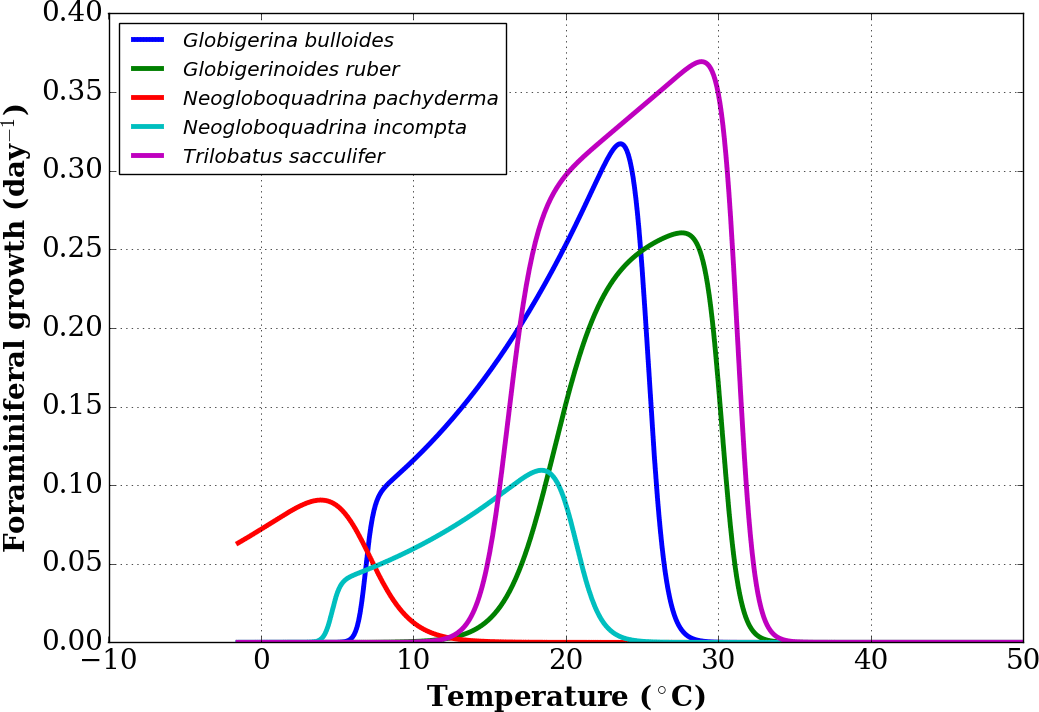
Figure 1Growth functions corresponding to Eq. (1) over the full temperature range considered, replotted from Lombard et al. (2009).
We compute the μ(T,k) coefficient for all values of in the World Ocean, T being a 4-D variable of space and time. This, in turn, gives us the growth rate of the different foraminifer species considered in a four-dimensional space as
To avoid numerical issues in the code, we limit the value of μ(T,k) on the low end as follows:
Given a four-dimensional input field for oceanic temperatures and δ18O of seawater, the equilibrium inorganic calcite δ18O value can be computed from the temperature equation of Kim and O'Neil (1997). Here, we use the quadratic approximation of that equation given in Bemis et al. (1998):
where T0=16.1 ∘C, and a=0.09, δ18Osw is the seawater δ18O. Since the seawater temperature (∘C) and δ18Osw (permil) are inputs, we can solve this equation to determine the value of δ18Oc. With the discriminant of the second-degree equation being
it becomes
where the constant, 0.27, correction (Hut, 1987) accounts for the difference in the reference scales of seawater (permil versus Vienna mean standard ocean water – V-SMOW) and calcite (permil versus V-PDB).
In previous studies, we and others (Caley et al., 2014; Werner et al., 2016) computed the above δ18O equilibrium value, averaged over time and the surface layer (typically the first 50 m) to compare model results and measured δ18Oc from planktonic foraminifers. In the following, we will refer to this method as the “old method”, written formally as
where nt is the number of time steps, nz the number of vertical levels and zb the maximum depth.
The formalism used clearly expresses the fact that the old method is not species-specific nor season-specific since all time steps and vertical levels are averaged with the same weight. In contrast, the FAME method weighs the δ18Oc both in time and in the horizontal and vertical space according to the population abundances using the foraminifer growth formula (1). We thus write
where zb(k) is dependent on the species and constrained by core-top data (see below).
Using this set of equations, for any given seawater temperature and δ18O provided as a four-dimensional field and a given species k, we compute this species' δ18Oc over x,y (latitude, longitude) coordinates.
It should be clearly understood that this approach is not able and does not attempt to determine the relative abundances of the different species. Instead FAME provides a simplified approach to compute the δ18Oc of a generic population of foraminifers if environmental conditions permit its growth. From a model–data perspective, this approach enables one to compute the calcite δ18O for a given species, were it to exist in the sedimentary record. Due to the limitations set by Eq. (3), no calcite isotopic content is computed if μ′ is zero, and hence these areas will be masked out in the following.
2.2 Growth function uncertainties
In the original work of Lombard et al. (2009), 95 % confidence intervals were shown per species' growth functions, but no equation was given for them. In order to nonetheless estimate the bias introduced in FAME by using the given functions, we combined the different possible values for the parameters of the growth functions to obtain functions that are close to the 95 % confidence intervals mentioned for most species and larger than the 95 % confidence intervals for others. This results in an upper and lower growth function for each species, as shown in Fig. A1, where the original data points of Lombard et al. (2009) are also given.
2.3 Reference datasets
In an attempt to validate the FAME approach, we apply its methodology to reference datasets, close to present-day observations. The first necessary step is the computation of a reference δ18Oc field as obtained when forced by climatological data.
For seawater temperature, we use the World Ocean Atlas 2013 (WOA13) (Locarnini et al., 2013) data at a monthly resolution. Considering that there is no equivalent seawater oxygen-18 gridded dataset available in the World Ocean Atlas fields and that the existing NASA Goddard Institute for Space Studies (GISS) gridded dataset (LeGrande and Schmidt, 2006) presents large deviations with respect to the seawater oxygen-18 (δ18Osw) raw data in numerous locations, we derived a δ18Osw dataset based on seawater salinity to δ18Osw relationships. This dataset is built in two steps: (a) derivation of regional δ18Osw – salinity relationships from GISS δ18Osw and salinity (Schmidt et al., 1999) clustered by oceanic regions, and (b) computation of a δ18Osw field based on the World Ocean Atlas 2013 (Zweng et al., 2013) salinity fields. The resulting field is at the World Ocean Atlas spatial resolution and is used as reference seawater oxygen-18 in the following. Details on the derivation of the δ18Osw dataset are given in Appendix A.
Ganssen and Kroon (2000); Anand et al. (2003); Kuroyanagi and Kawahata (2004); Farmer et al. (2007)Pak and Kennett (2002); Pak et al. (2004); Kuroyanagi and Kawahata (2004); von Langen et al. (2005)Ganssen and Kroon (2000); Anand et al. (2003); Kuroyanagi and Kawahata (2004); Farmer et al. (2007)Bauch et al. (2002); Ganssen and Kroon (2000); Pak and Kennett (2002); Pak et al. (2004); Kuroyanagi and Kawahata (2004)Kohfeld et al. (1996); Bauch et al. (1997, 2002); Simstich et al. (2003); Kuroyanagi and Kawahata (2004)Table 1 Maximum depth per species as computed from the optimization procedure. zb is the depth yielding the smallest difference to the MARGO Late Holocene data (Waelbroeck et al., 2005). We computed a confidence interval corresponding to a change of ±0.1 permil in the mean error. The ∞ sign indicates that no value of zb within the range yields the desired ±0.1 permil change.
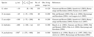
1 An encrustation term of +0.1 permil is taken into account in the case of N. pachyderma (see text).
As an independent test of the FAME results, we use the planktonic δ18Oc measurements from the Multiproxy Approach for the Reconstruction of the Glacial Ocean surface (MARGO) Late Holocene dataset (Waelbroeck et al., 2005) restricted to high chronozone quality levels (i.e., levels 1 to 4). A few errors have been corrected in the published dataset: these concern the suppression of 10 Neogloboquadrina incompta (or N. pachyderma right) data points from the Nordic Seas where only Neogloboquadrina pachyderma should have been listed, and one outlier N. pachyderma value with no age control that was erroneously listed as having a level-4 chronozone quality. The corrected version of MARGO Late Holocene planktonic oxygen-18 dataset is available in the Supplement.
As a result, the dataset used in the present study contains 248 values for Neogloboquadrina pachyderma, 128 values for Globigerina bulloides, 59 values for Neogloboquadrina incompta, 135 values for Globigerinoides ruber and 51 values for Globigerinoides sacculifer. In the remainder of the paper and following the genus reassignment of Spezzaferri et al. (2015), we will refer to the latter as Trilobatus sacculifer.
2.4 Calculation of the best-fitting maximum depth per foraminifer species
In Eq. (8), the maximum depth of integration per foraminifer species, zb(k), is a free parameter and needs to be determined. We have chosen to calculate it as the depth where the δ18Oc simulated by FAME driven by the World Ocean Atlas 2013 temperature and derived seawater δ18O datasets is closest on average to MARGO Late Holocene δ18Oc data. The rationale behind this choice is to specifically design FAME to enable model–data comparison with isotopic records from marine sediment cores.
To determine the optimal value of zb(k), we repeated successive runs of FAME with values of zb ranging from 1500 m to the surface along the standard World Ocean Atlas vertical grid. The only difference between the different species at this stage are the species-specific terms in the equations presented and the data of each species from the MARGO Late Holocene set. The results obtained through this optimization procedure are given in Table 1. The maximum depths of calcification derived this way are remarkably close to what is known from the ecology of G. ruber, N. incompta, T. sacculifer and G. bulloides (Berger, 1969; Bijma and Hemleben, 1994; Ortiz et al., 1995; Schiebel et al., 2002; Mortyn and Charles, 2003; Rebotim et al., 2017). Only in the case of N. pachyderma, the computed value of zb was much too deep (900 m) with respect to what studies based on opening–closing plankton nets show. Also, plankton haul studies have revealed that, whereas N. pachyderma seems to grow at relatively shallow depth, i.e., where the chlorophyll maximum is found, a calcite crust is added between ∼50 and 250 m, which greatly increases its mass (Kohfeld et al., 1996; Simstich et al., 2003). As a consequence, the δ18O of N. pachyderma collected in deep sediment traps and in surface sediment is systematically heavier than that of living non-encrusted N. pachyderma. To account for this effect, we have added a 0.1 permil “encrustation term” to our calculation of N. pachyderma calcite δ18O weighted by that species' culture-based growth rates. The encrustation term value has been chosen in order to simulate maximum depths in agreement with the literature. N. pachyderma simulated depth of maximum growth (Fig. 4e and Table 1) does indeed match very well the available observations. For instance, Fig. 4e shows a deepening of N. pachyderma depth of maximum growth from 0 to 30 m in the Greenland Sea to 100–350 m in the Norwegian Sea, in agreement with the apparent calcification depths reconstructed by Simstich et al. (2003).
Concerning T. sacculifer, although this species bears symbionts, and thus lives in the photic zone like G. ruber, it is known to produce calcite with higher δ18O values than G. ruber. These heavier δ18O values are thought to result from the accretion of gametogenetic calcite (for a certain unknown fraction of the shell mass) or from the precipitation of its final sac-like chamber deeper in the water column (Duplessy et al., 1981). This characteristic explains the deeper habitat depth computed for T. sacculifer versus G. ruber (maximum calcification depth estimates range from −200 to −75 m, best estimate of −100 m). Note that a deeper habitat for T. sacculifer than G. ruber is in agreement with observations (Table 1).
2.5 Evaluation of the model performance
2.5.1 Error distribution
Since the depth parameter was constrained using the MARGO Late Holocene dataset by error minimization, it is not surprising that the errors obtained with FAME are very small on average for each species considered (Fig. 2). The error distribution obtained with FAME is very similar to the one obtained with the simple surface equilibrium assumption for the two species closest to the surface (G. ruber and N. incompta). For deeper dwellers (T. sacculifer, G. bulloides & N. pachyderma), FAME results are better than those obtained with the old method, as expected, since deeper layers in the ocean are accounted for.
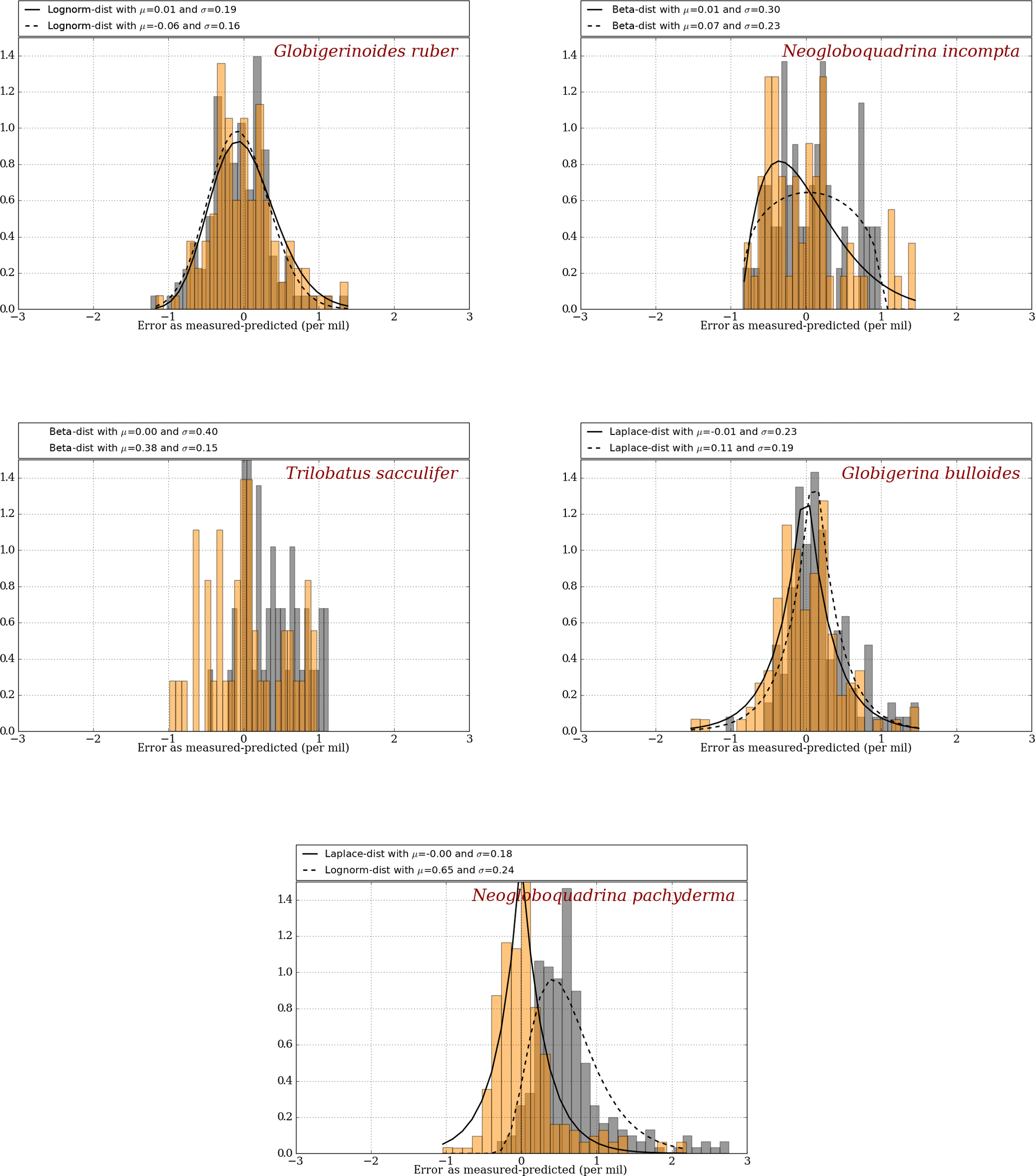
Figure 2Error distribution for the “old method” (grey) and the “FAME method” (orange) using climatological datasets as compared to MARGO Late Holocene dataset (Waelbroeck et al., 2005). Best-fitting distributions are calculated and plotted as a solid line for the FAME method and as a dashed line for the old method, except for T. sacculifer, for which the small number of available data points yields a poor fit both for FAME and the old method. The mean and deviation are given for FAME and the old method at the top of each panels.
2.5.2 Robustness of results
To test the robustness of our calibration in depth or error distribution, we performed a full set of additional analyses using the lower and upper growth functions as presented in Fig. A1, introduced here above.
Regarding depth calibration, we find our results to be largely insensitive to the use of these upper-bound and lower-bound values for the growth functions. Specifically, the uncertainty in the maximum growth depth is largest on N. pachyderma (range of 475 to 600 m) and G. bulloides (400 to 450 m). It is somewhat smaller for T. sacculifer (100 to 125 m) and N. incompta (60 to 65 m). There is no impact for G. ruber.
Another method to check the impact of the uncertainty in the growth functions on our δ18Oc results is by keeping maximum computed depths constant and looking at the impact of the growth function on the mean difference between simulated and MARGO δ18Oc values shown in Fig. 2. When doing so (not shown), the resulting change is lower than 0.1 permil for all individual species. It therefore shows that our results are very robust and largely insensitive to the errors arising in the growth functions used (Lombard et al., 2009).

Figure 3 Model–data comparison of species' abundances. Ocean regions where FAME predicts that the species is present at some time of the year () are plotted in blue, with shades of blue indicating the number of months of presence. Overlaid are the MARGO Late Holocene data (quality levels 1–4) species' abundance data, plotted using the yellow–white to dark red color bar and given in percent. A qualitative correspondence between simulated FAME presence/absence and the occurrence of 10 % level in the difference species is noted.
2.5.3 Geographical distribution
To further check our methodology against the MARGO Late Holocene dataset, we compare the zone of presence of each species predicted by FAME (grossly determined by μ′) with the observed reported abundances in the MARGO dataset (restricted to chronology quality values 1–4). As noted above, we cannot predict the relative abundance of each species. However, the method determines the species' absence or presence.
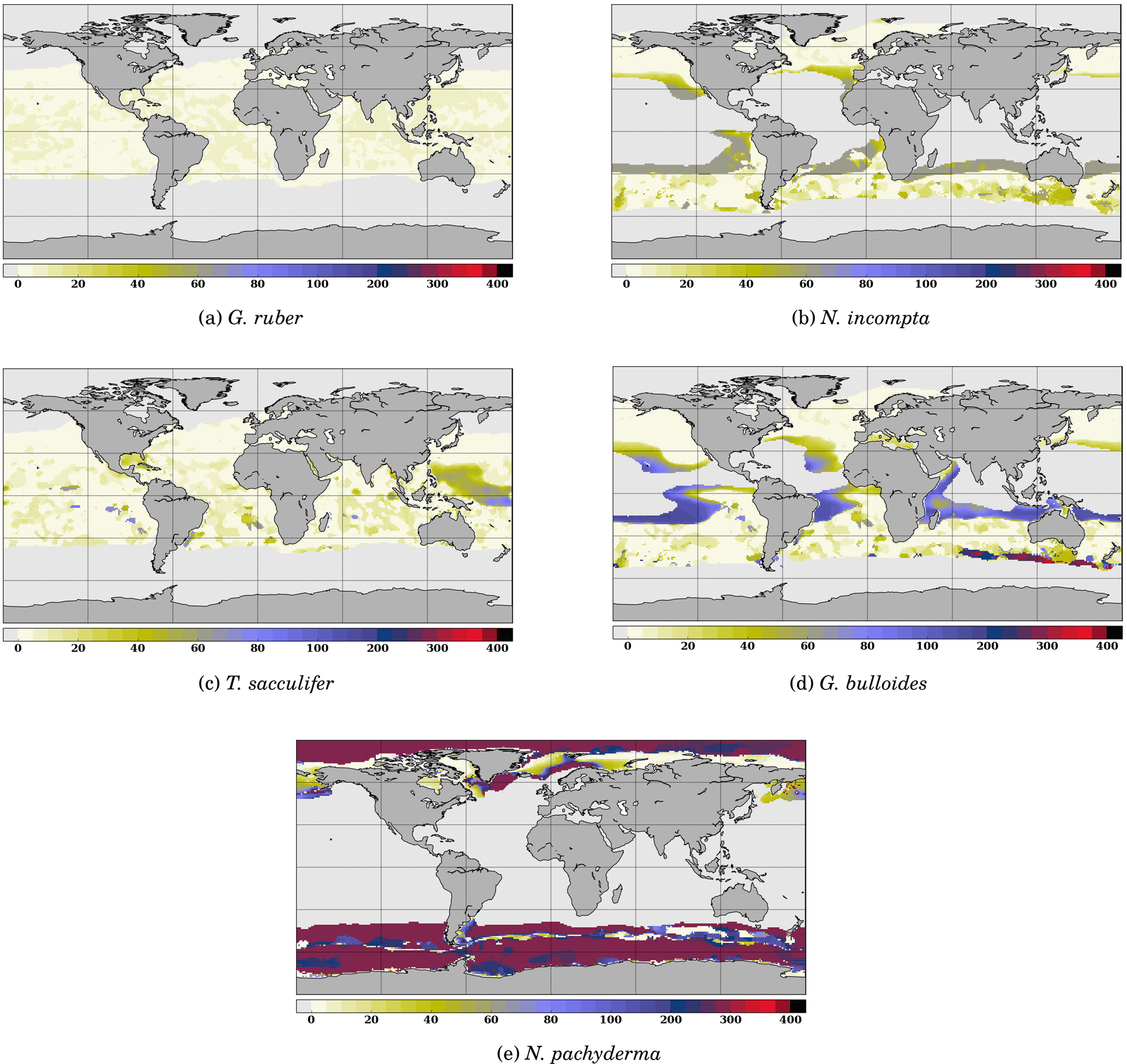
Figure 4 Depth of maximum growth for the species considered for the month of July. The color scale shows the depth in meters. Oceanic areas left in white correspond to areas where growth rates are below the threshold defined in Eq. (3).
The results presented in Fig. 3 show that, despite the exceptional simplicity of our approach, FAME predicts relatively well the spatial limits of the area occupied by each species. The two species whose presence distribution is best predicted are again G. bulloides and N. pachyderma, both showing a quite remarkable model–data match of the transition zones from presence to absence. N. incompta and G. ruber also show quite satisfactory results, with only a few outliers in specific areas: FAME computes overextended coverage of N. incompta in the Gulf of Guinea and of G. ruber along the coast of Namibia.
The computed spatial coverage of T. sacculifer is slightly too extended towards high northern and possibly southern latitudes. The very low number of high-quality dated data points in the latter area prevents a definitive conclusion. Also, specific zones, consistent for several species, may be noted, such as the Benguela upwelling regions where FAME fails to predict the absence of T. sacculifer and G. ruber.
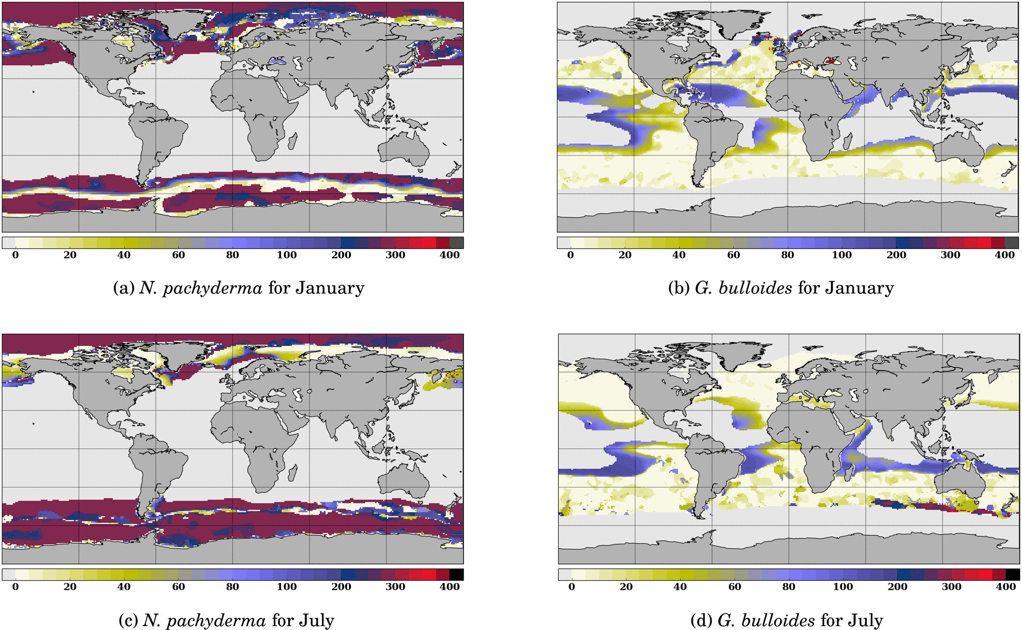
Figure 5 Comparison of the depth of maximum growth for N. pachyderma and G. bulloides for January and July. Color scale is as in Fig. 3.
One possible explanation for this mismatch could be the impact of increased nutrient availability on observed abundances as a consequence of the upwelling systems, whereas nutrients are at present ignored in the FAME approach. Another possibility could be the quality of the vertical oceanic structure obtained from the World Ocean Atlas in those upwelling regions. Finally, it should be noted that our comparison ignores the natural interannual variability since we are using climatologies. The interannual variability involves changes in the location of the fronts and currents, and thus bears the potential of shifting the spatial boundaries between the different foraminifer species.
Further discussion of the abundance comparison including all data points from the MARGO Late Holocene dataset regardless of the dating quality is given in Appendix B.
To further investigate the functioning of the FAME model, it is useful to consider the spatial distribution of the depth at which each species' growth is maximum. An example is given for the month of July in Fig. 4. It clearly shows that even though the maximum depth allowed for each species is fixed through the zb(k) parameter, the predicted/computed calcification depth varies according to the location in the World Ocean. Except for G. ruber which always calcifies in the topmost ocean layers, the depth of maximum growth exhibits large spatial variations, notably at the edge of the species' domains; in July, this is particularly marked in the case of G. bulloides and N. pachyderma (Fig. 4d and e).
Likewise, it is useful to consider the seasonal variations in the depth of maximum growth for a given species. We propose to highlight this aspect for the two species that show the largest variations: N. pachyderma and G. bulloides at two extreme months (January and July) (Fig. 5). For both species, the area of computed non-zero contribution varies along the year, with an expansion (reduction) of the area occupied by N. pachyderma in the Northern Hemisphere in January (July), while the regions occupied by G. bulloides shift towards higher (lower) latitudes in the Northern Hemisphere in July (January). These seasonal changes are a direct response of these species' preferred habitat to temperature. FAME thus mechanistically predicts the adaptation of planktonic foraminifer depth habitat to maintain optimal living conditions. For instance, Fig. 5b and d clearly show that G. bulloides is predicted to dwell deeper at low latitudes when surface temperature rises above its preferred temperature range. Similarly, Fig. 5b and d show that G. bulloides is present at higher northern latitudes in July than in January, so that the growing season actually tracks the species' preferred living conditions, as observed (Jonkers and Kucera, 2015).
2.5.4 Effect of a large climatic change on the computed oxygen-18 content of the calcite
Though FAME gives realistic results when forced by atlas data, it is mostly designed to retrieve the species-specific effect of climate change on the recorded δ18Oc. To highlight the effect of seasonal and vertical weighting of the δ18Oc signal computed by FAME, we have performed a simplified experiment showing the effect of a change in the foraminifers' living conditions on their δ18Oc signal.
To simulate a change in climatic conditions, we apply a homogeneous 4 ∘C decrease to the WOA13 sea temperature dataset and compute the anomaly in δ18Oc between that new cold state and the original one for each species, as well as for the surface equilibrium approach (Fig. 6). This anomaly is noted Δ18Oc in what follows.
Applying a spatially homogeneous temperature change should result is a quasi-homogeneous temperature change in the equilibrium calcite Δ18Oc, following Eq. (6). It is indeed what is obtained in Fig. 6e, with Δ18Oc values between 0.8 in the tropics and 1 permil at high latitudes. When applying the FAME equations, we obtain large spatial variations in Δ18Oc with values down to −0.75 and up to 1 permil. All species share a common pattern of lower Δ18Oc at the border of their living domain and close to equilibrium values at the center of their living domain. More specifically, the smallest differences to the equilibrium are recorded by N. pachyderma and the largest, negative, differences are computed for G. bulloides. The species with the smallest vertical living range, G. ruber, has the most homogeneous distribution. The range of values (minimum to maximum) is always close to 1 permil with the exception of G. bulloides that presents a total range of 1.6 permil. This large range of Δ18Oc for G. bulloides is a consequence of its growth over a large range of temperatures (Eq. 1). In general, the maximum simulated Δ18Oc values are systematically 0.1 to 0.2 permil lower than the equilibrium value.
This simple scenario, though unrealistic with respect to actual climatic applications, shows the potential of FAME to unravel the climatic signal embedded in multispecies isotopic records and thus opens the door to transient climate–data intercomparison where the species' specific behavior is taken into account.
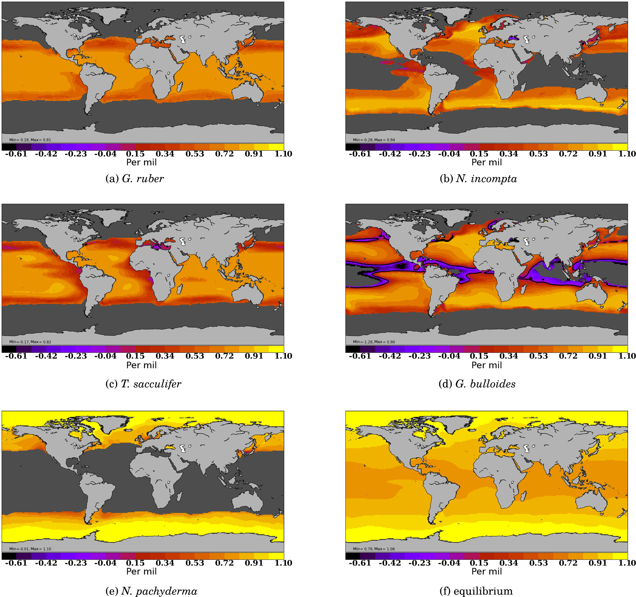
Figure 6δ18Oc response to a horizontally and vertically homogeneous 4 ∘C cooling applied to the WOA13 dataset, Δ18Oc. Results are expressed in permil for each species (a–d) and for the equilibrium surface calcite approach.
We developed the FAME (Foraminifers As Modeled Entities) module to account for planktonic foraminifer species-specific habitat when computing their calcite oxygen-18. In contrast to models predicting the abundance of planktonic foraminifers, FAME only aims at predicting the presence or absence of a given species and its oxygen-18 value. FAME is only forced by hydrographic data and uses a very limited number of parameters, almost all derived from culture experiments. Taken together, these characteristics make FAME a uniquely simple and robust model for predicting changes in the oxygen-18 of commonly used planktonic foraminifer species in response to changing climatic conditions. FAME performance is evaluated using MARGO Late Holocene planktonic foraminifer δ18Oc and abundance datasets. We show that FAME predicts remarkably well the presence/absence of G. ruber, N. incompta, N. pachyderma and G. bulloides over most of the World Ocean, while yielding a slightly less good prediction of T. sacculifer presence/absence. Investigating the simulated seasonal pattern, we show that the predicted growing season and habitat depth track the species' preferred living conditions, as observed in plankton hauls and sediment-trap data. Finally, the application of FAME to a simple cooling scenario demonstrates that computed changes in species-specific δ18Oc are much more spatially variable than the computed change in equilibrium surface calcite. Coupling the FAME module to isotope-enabled climate models makes it possible for the first time to extract the climatic information contained in isotopic time series measured on different planktonic species at the same location. This opens the possibility to better reconstruct the evolution of the upper water column structure than ever before, notably over climate transitions.
The FAME module has been developed in Python version 3 and tested under version 3.5.1. The code is made available under the GNU General Public License https://www.gnu.org/licenses/gpl.html (last access: 30 August 2018) and is uploaded in the Supplement of this paper.
The World Ocean Atlas datasets used are available to all users directly from the provider. Derivation of the reference δ18Osw dataset is detailed in Appendix A. The masks' file used in the latter procedure is provided in the Supplement to the paper.
We constructed our reference δ18Osw dataset at World Ocean Atlas standard resolution (1∘ grid) through a three-step methodology: (a) construction of an appropriate basin mask to allow clustering the GISS global dataset regionally, (b) derivation of δ18Osw – salinity relationships for each of these basins and (c) use of these relationships to obtain a δ18Osw field at WOA spatial resolution.
A1 Construction of the basin masks
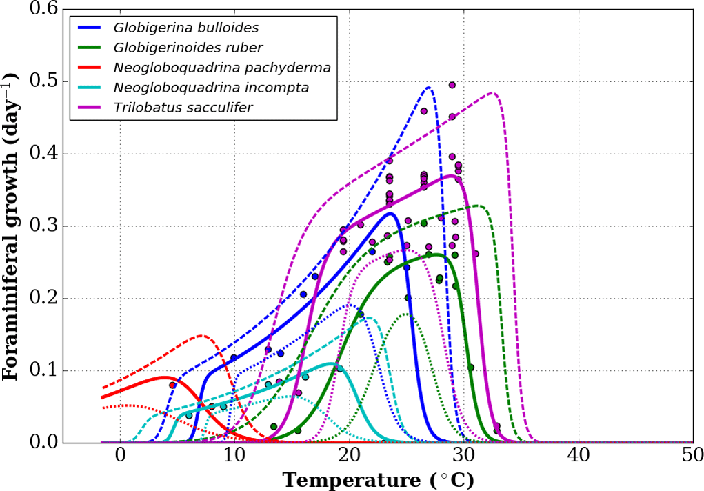
Figure A1Growth functions corresponding to Eq. (1) over the full temperature range considered, with added lower-range and upper-range curves (respectively, short and long dashed curves) chosen to mimic the 95 % confidence interval of Lombard et al. (2009). Data points are the original data obtained by Lombard et al. (2009).

Figure A2Basin masks as defined in the WOA standard mask file (a) and in FAME (b) on the same 1∘ resolution grid. Values correspond to the basins defined in Table A1.
Table A1Comparative list of basin masks in WOA and FAME. The “value” field provides the integer value used in the netCDF file to specify the respective basin on the WOA grid.
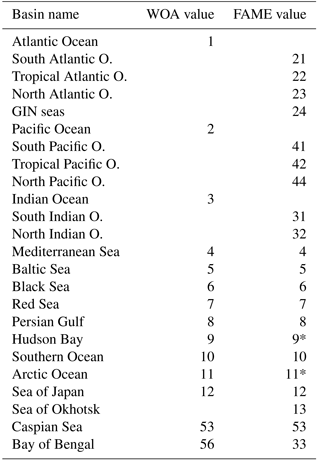
The “*” symbol highlights the regions where FAME and WOA regions do not cover the same area (see text).
Our native resolution being the 1∘ regular grid of the World Ocean Atlas, we first retrieved the available basin mask file on that grid from the National Oceanic and Atmospheric Administration (NOAA) website https://www.nodc.noaa.gov/OC5/woa13/masks13.html (last access: 5 October 2016) and converted it to a netCDF format file (http://www.unidata.ucar.edu/software/netcdf, last access: 30 August 2018). The basins defined in the WOA base mask did not perfectly fit our purpose; we hence modified the masks to isolate some particular regions where the δ18Osw and salinities are specific (e.g., Sea of Okhotsk) or merge some regions of the WOA mask into larger ensembles (e.g., Hudson Bay). A summary of the basins in the original file and in ours is given in Table A1. The Pacific and Atlantic oceans were split into south, north and tropical parts, based on boundaries at 30∘ north and south, respectively. The Indian Ocean has been only split in two: north and south using the 30∘ south boundary. The Bay of Bengal has been kept a separated basin as in the original file. The Greenland–Iceland–Norwegian (GIN) seas were made a separated basin from the Arctic Ocean, using the boundaries at 80∘ north and at 20∘ east. We also extended the Hudson Bay mask area to include the Hudson Strait and Ungava Bay, since these do not represent the same water mass properties as the North Atlantic Ocean. The limit used is −64.5∘ west, corresponding to the southern tip of Resolution Island on the grid given. Finally, the same procedure was applied to define the Sea of Okhotsk, using the official definition of the International Hydrographic Organization (IHO SP-23() IHO SP-23: Limits of Oceans and Seas, International Hydrographic Organization, Imp. Monégasque, Monte Carlo, special Publication no. 23, 1953). The results of this whole procedure are shown in Fig. A2. In Table A1, some values are annotated with a “*” to highlight basins having the same value in FAME as in the standard WOA but covering a different area: the Arctic Ocean from which the GIN seas have been taken out in FAME, Hudson Bay which covers a part of the former Atlantic basin of the WOA given its aforementioned expansion to the Hudson Strait and Ungava Bay.
The netCDF data file resulting from this procedure is provided in the Supplement to the paper.
Computation of the δ18Osw – salinity relationships
The basins defined in the previous section are then used to cluster the raw data, δ18Osw and salinity, of the GISS database (Schmidt et al., 1999) in the respective basins. Furthermore, only data locations where both δ18Osw and salinity are given in the original database for depths less than 200 m are retained under the additional constraint that depth of the ocean should be more than 175 m. The latter are to ensure that the values are representative of high sea values and not coastal areas, possibly under fluvial influence. Additionally, all values below 5 permil in salinity are ignored for all basins. Lastly, for two basins (North Atlantic and Bay of Bengal), the existence of two different slopes where only one corresponds to open-ocean conditions renders necessary the addition of one additional condition to keep only the latter. We thus added a limit at 27 permil in salinity for those two basins.
The resulting slopes, intercept and correlation coefficients are given in the Table A2. Using those relationships, we further compute the δ18Osw in the WOA geographical grid from the WOA salinity fields.
Table A2 Values obtained for the δ18Osw – salinity relationships.
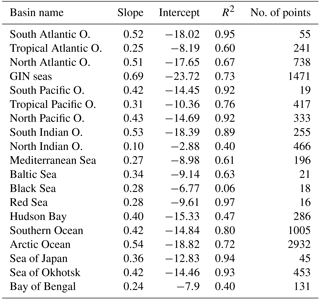

Figure B1 Model–data comparison of species' abundances. Ocean regions where FAME predicts that the species is present at some time of the year () are plotted in blue, with shades of blue indicating the number of months of presence. Overlaid are the MARGO Late Holocene data (all quality levels) species' abundance data, plotted using the yellow–white to dark red color bar and given in percent. A qualitative correspondence between simulated FAME presence/absence and the occurrence of 10 % level in the difference species is noted.
In the main text, we have only compared the results of FAME to the data points in the MARGO Late Holocene database that were characterized by high chronological control quality. Since this drastically restricts the geographical extent covered by MARGO data, and in the interest of completeness, we propose here a short discussion based on all points of the MARGO Late Holocene database, regardless of their chronological control quality. The interest of Fig. B1 is to provide some information in the Southern, Pacific and Indian Ocean regions that are largely void of points in the previous figure. While the bulk of the conclusions given in the main text is unchanged by this new comparison, we may highlight the following.
The unsorted distribution for G. ruber is not very different from the one described above, albeit with a good definition of the Southern Ocean abundance limit where FAME results are in good accordance with MARGO. Also, one may note a series of points without the presence of G. ruber in the equatorial Pacific in MARGO, an aspect which is not predicted by FAME. However, these points are mingled with points with G. ruber presence in the MARGO database, indicating they could be an artifact resulting from the presence of older sedimentary material in the unsorted MARGO database; it is thus difficult to draw a firm conclusion.
Regarding N. incompta, the picture is pretty much the same as described in the main text to the exception of a number of mismatching sites in the tropical and midlatitudes in all Southern Ocean basins (Pacific, Indian and Atlantic).
The distribution for T. sacculifer shows a clear latitudinal mismatch of the limit of presence/absence when comparing the FAME results to the unsorted MARGO dataset. It seems obvious that the latitudinal spread of G. ruber in FAME should be considered as too extended in the middle to high latitudes in both hemispheres.
The joint comparison of unsorted G. ruber and T. sacculifer distributions points to the existence of consistent zones where FAME does not predict the absence of those two species. This was noted earlier for the Benguela upwelling region. It is also visible here for the Peru–Chile upwelling and the eastern equatorial Pacific. All these zones correspond to upwelling regions (e.g., Mackas et al., 2006) and are characterized by strong contrasts in surface water properties with respect to the surrounding regions, large interannual and intra-seasonal variability, and high phytoplankton production. The existence of this consistent pattern in upwelling regions in the unsorted database confirms that G. ruber and T. sacculifer distributions are not well simulated in upwelling regions, either because nutrients are presently not accounted for in FAME or because the increased nutrient availability and/or the vertical structure of oceanic physical properties is not faithfully depicted in the 1∘ resolution WOA13 dataset we used in input.
The unsorted distribution for G. bulloides still presents an excellent match for the limits but with some discrepancies in the equatorial and tropical latitudes; albeit MARGO unsorted data do not present a large regional consistency outside the northern coast of Brazil (where FAME also predicts the absence of G. bulloides).
Aside from some minor mismatches in the southern Indian Ocean, the conclusions for N. pachyderma are also largely unaffected by the use of all the points from the MARGO database.
To conclude, the use of all the data points regardless of the quality of the chronological control in the MARGO Late Holocene database does not add much new information, especially since the data points should be considered with caution as they could correspond to a different climate regime than the Late Holocene.
The supplement related to this article is available online at: https://doi.org/10.5194/gmd-11-3587-2018-supplement.
DMR and CW designed the study. DMR wrote the code and performed the experiments with regular input from CW. DMR wrote the manuscript with contribution form all co-authors.
The authors declare that they have no conflict of interest.
This is a contribution to the ACCLIMATE ERC project. The research leading to
these results has received funding from the European Research Council under
the European Union's Seventh Framework Programme (FP7/2007-2013; grant
agreement no. 339108). We thank Lukas Jonkers and Michal Kucera for fruitful
discussions on earlier versions of this work.
Edited by: Sandra Arndt
Reviewed by: two anonymous referees
Anand, P., Elderfield, H., and Conte, M. H.: Calibration of Mg/Ca thermometry in planktonic foraminifera from a sediment trap time series, Paleoceanography, 18, 1–16, https://doi.org/10.1029/2002PA000846, 2003. a, b
Bauch, D., Carstens, J., and Wefer, G.: Oxygen isotope composition of living Neogloboquadrina pachyderma (sin.) in the Arctic Ocean, Earth Planet. Sci. Lett., 146, 47–58, https://doi.org/10.1016/S0012-821X(96)00211-7, 1997. a, b
Bauch, D., Erlenkeuser, H., Winckler, G., Pavlova, G., and Thiede, J.: Carbon isotopes and habitat of polar planktic foraminifera in the Okhotsk Sea: the ‘carbonate ion effect’ under natural conditions, Marine Micropaleontology, 45, 83–99, https://doi.org/10.1016/S0377-8398(02)00038-5, 2002. a, b
Bé, A. W. H. and Tolderlund, D. S.: Distribution and ecology of living planktonic foraminifera in surface waters of the Atlantic and Indian Oceans, in: The Micropaleontology of Oceans, edited by: Funnel, B. M. and Riedel, W. R., 105–149, Cambridge University Press, Cambridge, United Kingdom, 1971. a
Bemis, B. E., Spero, H. J., Bijma, J., and Lea, D. W.: Reevaluation of the oxygen isotopic composition of planktonic foraminifera: Experimental results and revised paleotemperature equations, Paleoceanography, 13, 150–160, https://doi.org/10.1029/98PA00070, 1998. a
Berger, W. H.: Ecologic patterns of living planktonic Foraminifera, Deep Sea Res. Ocean. Abstr., 16, 1–24, https://doi.org/10.1016/0011-7471(69)90047-3, 1969. a, b
Bijma, J. and Hemleben, C.: Population dynamics of the planktic foraminifer Globigerinoides sacculifer (Brady) from the central Red Sea, Deep Sea Res. Pt. I, 41, 485–510, https://doi.org/10.1016/0967-0637(94)90092-2, 1994. a, b
Caley, T., Roche, D. M., Waelbroeck, C., and Michel, E.: Oxygen stable isotopes during the Last Glacial Maximum climate: perspectives from data-model (iLOVECLIM) comparison, Clim. Past, 10, 1939–1955, https://doi.org/10.5194/cp-10-1939-2014, 2014. a, b
Deuser, W. G.: Seasonal variations in isotopic composition and deep-water fluxes of the tests of perennially abundant planktonic foraminifera of the Sargasso Sea: results from sediment-trap collections and their paleoceanographic significance, J. Foraminiferal Res., 17, 14–27, 1987. a
Duplessy, J.-C., Lalou, C., and Vinot, A. C.: Differential Isotopic Fractionation in Benthic Foraminifera and Paleotemperatures Reassessed, Science, 168, 250–251, 1970. a
Duplessy, J. C., Bé, A. W. H., and Blanc, P. L.: Oxygen and carbon isotopic composition and biogeographic distribution of planktonic foraminifera in the Indian Ocean, Palaeogeogr. Palaeoclimatol. Palaeoecol., 33, 9–46, https://doi.org/10.1016/0031-0182(81)90031-6, 1981. a
Emiliani, C.: Depth habitats of some species of pelagic foraminifera as indicated by oxygen isotope ratios, Am. J. Sci., 252, 149–158, 1954. a, b
Emiliani, C.: Pleistocene temperatures, J. Geol., 63, 538–577, 1955. a
Ezard, T. H. G., Edgar, K. M., and Hull, P. M.: Environmental and biological controls on size-specific d13C and d18O in recent planktonic foraminifera, Paleoceanography, 30, 151–173, https://doi.org/10.1002/2014PA002735, 2015. a
Fairbanks, R. G. and Wiebe, P. H.: Foraminifera and chlorophyll maxima: vertical distribution, seasonal succession, and paleoceanographic significance, Science, 209, 1524–1526, 1980. a
Farmer, E. C., Kaplan, A., de Menocal, P. B., and Lynch-Stieglitz, J.: Corroborating ecological depth preferences of planktonic foraminifera in the tropical Atlantic with the stable oxygen isotope ratios of core top specimens, Paleoceanography, 22, 1–14, https://doi.org/10.1029/2006PA001361, 2007. a, b
Fraile, I., Schulz, M., Mulitza, S., and Kucera, M.: Predicting the global distribution of planktonic foraminifera using a dynamic ecosystem model, Biogeosciences, 5, 891–911, https://doi.org/10.5194/bg-5-891-2008, 2008. a, b, c
Ganssen, G. M. and Kroon, D.: The isotopic signature of planktonic foraminifera from NE Atlantic surface sediments: implications for the reconstruction of past oceanic conditions, J. Geol. Soc., 157, 693–699, https://doi.org/10.1144/jgs.157.3.693, 2000. a, b, c
Hut, G.: Consultant's group meeting on stable isotope reference samples for geochemical and hydrological investigations, International Atomic Energy Agency, 42, 1–43, 1987. a
IHO SP-23: Limits of Oceans and Seas, International Hydrographic Organization, Imp. Monégasque, Monte Carlo, special Publication no. 23, 1953. a
Jones, J. I.: Significance of the distribution of planktonic foraminifera in the equatorial Atlantic undercurrent, Micropaleontology, 13, 489–501, 1967. a
Jonkers, L. and Kucera, M.: Global analysis of seasonality in the shell flux of extant planktonic Foraminifera, Biogeosciences, 12, 2207–2226, https://doi.org/10.5194/bg-12-2207-2015, 2015. a, b
Jonkers, L., van Heuven, S., Zahn, R., and Peeters, F. J. C.: Seasonal patterns of shell flux, d18O and d13C of small and large N. pachyderma (s) and G. bulloides in the subpolar North Atlantic, Paleoceanography, 28, 164–174, https://doi.org/10.1002/palo.20018, 2013. a
Kim, S.-T. and O'Neil, J. R.: Equilibrium and nonequilibrium oxygen isotope effects in synthetic carbonates, Geochim. Cosmochim. Ac., 61, 3461–3475, https://doi.org/10.1016/S0016-7037(97)00169-5, 1997. a
Kohfeld, K. E., Fairbanks, R. G., Smith, S. L., and Walsh, I. D.: Neogloboquadrina pachyderma (sinistral coiling) as paleoceanographic tracers in polar oceans: evidence from northeast water polynia plankton tows, sediment traps, and surface sediments, Paleoceanography, 11, 697–699, 1996. a, b, c
Kooijman, S.: Dynamic Energy and Mass Budgets in Biological Systems, Cambridge university press, 2000. a
Kuroyanagi, A. and Kawahata, H.: Vertical distribution of living planktonic foraminifera in the seas around Japan, Marine Micropaleontol., 53, 173–196, https://doi.org/10.1016/j.marmicro.2004.06.001, 2004. a, b, c, d, e
LeGrande, A. and Schmidt, G.: Global gridded data set of the oxygen isotopic composition in seawater, Geophys. Res. Lett., 33, L12604, https://doi.org/10.1029/2006GL026011, 2006. a
Lidz, B., Kehm, A., and Miller, H.: Depth Habitats of Pelagic Foraminifera during the Pleistocene, Nature, 217, 245–247, https://doi.org/10.1038/217245a0, 1968. a
Locarnini, R. A., Mishonov, A. V., Antonov, J. I., Boyer, T. P., Garcia, H. E., Baranova, O. K., Zweng, M. M., Paver, C. R., Reagan, J. R., Johnson, D. R., Hamilton, M., and Seidov, D.: World Ocean Atlas 2013, Volume 1: Temperature, in: World Ocean Atlas 2013, edited by: Levitus, S. and Mishonov, A., vol. 1, p. 40, NOAA Atlas NESDIS 73, 2013. a
Lombard, F., Labeyrie, L., Michel, E., Spero, H. J., and Lea, D. W.: Modelling the temperature dependent growth rates of planktic foraminifera, Mar. Micropaleontol., 70, 1–7, https://doi.org/10.1016/j.marmicro.2008.09.004, 2009. a, b, c, d, e, f, g, h, i, j, k
Lombard, F., Labeyrie, L., Michel, E., Bopp, L., Cortijo, E., Retailleau, S., Howa, H., and Jorissen, F.: Modelling planktic foraminifer growth and distribution using an ecophysiological multi-species approach, Biogeosciences, 8, 853–873, https://doi.org/10.5194/bg-8-853-2011, 2011. a, b, c
Mackas, D., Strub, P., Thomas, A., and Montecino, V.: Eastern regional ocean boundaries pan-regional overview, in: The Sea, edited by: Robinson, A. and Brink, K., vol. 14a, 21–60, Harvard University Press, Cambridge, Massachussetts, 2006. a
Mix, A. C.: The oxygen-isotope record of deglaciation, in: North America and adjacent oceans during the last deglaciation, edited by: Ruddiman, W. F. and Wright, H. E. J., vol. K-3 of The Geology of America, pp. 111–135, Geological Society of America, Boulder, Colorado, 1987. a, b, c, d, e
Mortyn, P. G. and Charles, C. D.: Planktonic foraminiferal depth habitat and d18O calibrations: Plankton tow results from the Atlantic sector of the Southern Ocean, Paleoceanography, 18, 1037, https://doi.org/10.1029/2001PA000637, 2003. a, b
Mulitza, S., Durkoop, A., Hale, W., Wefer, G., and Niebler, H. S.: Planktonic foraminifera as recorders of past surface-water stratification, Geology, 25, 335–338, https://doi.org/10.1130/0091-7613(1997)025<0335:PFAROP>2.3.CO;2, 1997. a
Ortiz, J. D., Mix, A. C., and Collier, R. W.: Environmental control of living symbiotic and asymbiotic foraminifera of the California Current, Paleoceanography, 10, 987–1009, https://doi.org/10.1029/95PA02088, 1995. a, b
Pak, D. K. and Kennett, J. P.: A FORAMINIFERAL ISOTOPIC PROXY FOR UPPER WATER MASS STRATIFICATION, J. Foraminiferal Res., 32, 319, https://doi.org/10.2113/32.3.319, 2002. a, b
Pak, D. K., Lea, D. W., and P., K. J.: Seasonal and interannual variation in Santa Barbara Basin water temperatures observed in sediment trap foraminiferal Mg/Ca, Geochem. Geophy. Geosy., 5, 1–18, https://doi.org/10.1029/2004GC000760, 2004. a, b
Pearson, P. N.: Oxygen Isotopes in Foraminifera: Overview and Historical Review, The Paleontological Society Papers, 18, 1–38, http://orca.cf.ac.uk/id/eprint/41988, 2012. a
Rebotim, A., Voelker, A. H. L., Jonkers, L., Waniek, J. J., Meggers, H., Schiebel, R., Fraile, I., Schulz, M., and Kucera, M.: Factors controlling the depth habitat of planktonic foraminifera in the subtropical eastern North Atlantic, Biogeosciences, 14, 827–859, https://doi.org/10.5194/bg-14-827-2017, 2017. a, b
Schiebel, R., Waniek, J., Zeltner, A., and Alves, M.: Impact of the Azores Front on the distribution of planktic foraminifers, shelled gastropods, and coccolithophorids, Deep Sea Res. Pt. II, 49, 4035–4050, https://doi.org/10.1016/S0967-0645(02)00141-8, 2002. a, b
Schmidt, G. A.: Forward modelling of carbonate proxy data from planktonic foraminifera using oxygen isotope tracers in a global ocean model, Paloeoceanography, 14, 482–497, 1999. a
Schmidt, G. A., Bigg, G. R., and Rohling, E. J.: Global Seawater Oxygen-18 Database – v1.22, available at: https://data.giss.nasa.gov/o18data (last access: May 2016), 1999. a, b
Simstich, J., Sarnthein, M., and Erlenkeuser, H.: Paired d18O signals of Neogloboquadrina pachyderma (s) and Turborotalita quinqueloba show thermal stratification structure in Nordic Seas, Mar. Micropaleontol., 48, 107–125, 2003. a, b, c, d
Spero, H. J.: Life history and stable isotope geochemistry of planktonic foraminifera, in: Isotope Paleobiology and Paleoecology, edited by: Norris, R. D. and Corfield, R. M., vol. 4, 7–36, The Paleontological Society Papers, 1998. a
Spero, H. J., Bijma, J., Lea, D. W., and Bemis, B. E.: Effect of seawater carbonate concentration on foraminiferal carbon and oxygen isotopes, Nature, 390, 497–500, https://doi.org/10.1038/37333, 1997. a
Spezzaferri, S., Kucera, M., Pearson, P., Wade, B., Rappo, S., Poole, C., Morard, R., and Stalder, C.: Fossil and Genetic Evidence for the Polyphyletic Nature of the Planktonic Foraminifera “Globigerinoides”, and Description of the New Genus Trilobatus, PloS ONE, 10, e0128108, https://doi.org/10.1371/journal.pone.0128108, 2015. a
von Langen, P. J., Pak, D. K., Spero, H. J., and Lea, D. W.: Effects of temperature on Mg/Ca in neogloboquadrinid shells determined by live culturing, Geochem. Geophy. Geosy., 6, 1–11, https://doi.org/10.1029/2005GC000989, 2005. a
Waelbroeck, C., Mulitza, S., Spero, H. J., Dokken, T., Kiefer, T., and Cortijo, E.: A global compilation of Late Holocene planktonic foraminiferal d18O: Relationship between surface water temperature and d18O, Quaternary Sci. Rev., 24, 853–868, https://doi.org/10.1016/j.quascirev.2003.10.014, 2005. a, b, c
Werner, M., Haese, B., Xu, X., Zhang, X., Butzin, M., and Lohmann, G.: Glacial-interglacial changes in H218O, HDO and deuterium excess – results from the fully coupled ECHAM5/MPI-OM Earth system model, Geosci. Model Dev., 9, 647–670, https://doi.org/10.5194/gmd-9-647-2016, 2016. a, b
Zweng, M., Reagan, J., Antonov, J., Locarnini, R., Mishonov, A., Boyer, T., Garcia, H., Baranova, O., Johnson, D., Seidov, D., and Biddle, M.: World Ocean Atlas 2013, Volume 2: Salinity, in: World Ocean Atlas 2013, edited by: Levitus, S. and Mishonov, A., vol. 2, p. 39, NOAA Atlas NESDIS 74, 2013. a
- Abstract
- Introduction
- Methodology
- Summary and conclusions
- Code availability
- Data availability
- Derivation of the a reference δ18Osw dataset
- Appendix B: Further discussion of predicted and observed planktonic foraminifer abundances
- Author contributions
- Competing interests
- Acknowledgements
- References
- Supplement