Observational operators for dual polarimetric radars in variational data assimilation systems (PolRad VAR v1.0)

We implemented two observational operators for dual polarimetric radars in two variational data assimilation systems: WRF Var, the Weather Research and Forecasting Model variational data assimilation system, and NHM-4DVAR, the nonhydrostatic variational data assimilation system for the Japan Meteorological Agency nonhydrostatic model. The operators consist of a space interpolator, two types of variable converters, and their linearized and transposed (adjoint) operators. The space interpolator takes account of the effects of radar-beam broadening in both the vertical and horizontal directions and climatological beam bending. The first variable converter emulates polarimetric parameters with model prognostic variables and includes attenuation effects, and the second one derives rainwater content from the observed polarimetric parameter (specific differential phase). We developed linearized and adjoint operators for the space interpolator and variable converters and then assessed whether the linearity of the linearized operators and the accuracy of the adjoint operators were good enough for implementation in variational systems. The results of a simple assimilation experiment showed good agreement between assimilation results and observations with respect to reflectivity and specific differential phase but not with respect to differential reflectivity.

1 Introduction

The Weather Research and Forecasting Model (WRF; Skamarock et al., 2008) is a widely used numerical weather model that was developed as a community model, and WRF Var, its data assimilation system (Barker et al., 2012), provides initial conditions for the model. NHM-4DVAR is a nonhydrostatic 4D-Var system for the Japan Meteorological Agency nonhydrostatic model (JMANHM; Saito, 2012) that functions at storm scale (Kawabata et al., 2007, 2014a). Many remote sensing data are available for NHM-4DVAR, such as the following: slant total delay, zenith total delay, and precipitable water vapor observed by global navigation satellite systems (GNSS; Kawabata et al., 2013); conventional radar data, including directly assimilated reflectivity data (Kawabata et al., 2011); and Doppler lidar data (Kawabata et al., 2014b). Because data assimilation associates observations with model fields, to make use of advanced observations, data assimilation methods need to be continuously developed and implemented into variational data assimilation systems.

Observations obtained by dual polarimetric radars are utilized by operational systems at many meteorological and hydrological operation centers (e.g., in the United States, France, Germany, and Japan) to improve the accuracy of quantitative precipitation estimation (QPE). These radars provide polarimetric parameters, including the horizontally polarized reflectivity factor (Z_H), the vertically polarized reflectivity factor (Z_V), differential reflectivity (Z_DR), and the specific differential phase (K_DP). Many QPE methods that use these parameters have been proposed (e.g., Jameson, 1991; Jameson and Caylor, 1994; Ryzhkov and Zrnić, 1995; Anagnostou et al., 2008; Kim et al., 2010; Ryzhkov et al., 2014; Adachi et al., 2015). Because QPE methods using dual polarimetric radar parameters are expected to be better than methods using single polarization radar data, we developed assimilation methods for dual polarimetric radar observations for both WRF Var and NHM-4DVAR. The objective of our study was thus to improve QPE, which was discussed in Bauer et al. (2015) in the context of data assimilation with high resolution and a rapid update cycle, and quantitative rainfall forecasts (QPF) through the use of better analysis fields obtained by the assimilation of dual polarimetric radar observations.

We chose an emulator (Zhang et al., 2001) and an estimator (Bringi and Chandrasekar, 2001) to use as forward operators after evaluating their accuracy (Kawabata et al., 2018). In addition, because both WRF Var and NHM-4DVAR consider only perturbations to rainwater in their tangent and adjoint models, our operators also deal only with rainwater and exclude ice particles. Although both the emulator of Jung et al. (2008a, b) and the estimator of Yokota et al. (2016) have been used previously as observational operators in ensemble Kalman filter data assimilation systems, to our knowledge, our study is their first implementation in variational assimilation systems. We refer to the current version of the operators as PolRad VAR v1.0.

The first author has mainly contributed to the WRF Var version of these operators developed over the rapid-update WRF 3D-Var system at the University of Hohenheim, Germany (see, e.g., Schwitalla et al., 2011; Schwitalla and Wulfmeyer, 2014; Bauer et al., 2015) and then to the version for NHM-4DVAR at the Meteorological Research Institute, Japan Meteorological Agency.

The scope of this paper is to provide the technical information on the observational operators and some evaluation results to help users understand the theoretical and practical aspects of the operators. The forward operators (space interpolator and variable converters) and their linearized (tangent linear) and transposed (adjoint) operators are described in Sect. 2. Section 3 describes the setup options of the observational operators, Sect. 4 presents verification and assimilation test results, and Sect. 5 is a summary.

2 Observational operators

In variational data assimilation systems, a cost function is defined and then iteratively minimized until its gradient becomes zero. The cost function and its gradient are defined as

$$\begin{array}{ll}{\displaystyle }& {\displaystyle }J\left(\mathbf{x}\right)={\displaystyle \frac{\mathrm{1}}{\mathrm{2}}}{\left(\mathbf{x}-{\mathbf{x}}^b\right)}^{\mathrm{T}}{\mathbf{B}}^{-\mathrm{1}}\left(\mathbf{x}-{\mathbf{x}}^b\right)\\ \text{(1)}& {\displaystyle }& {\displaystyle }+{\displaystyle \frac{\mathrm{1}}{\mathrm{2}}}{\left(H\left(\mathbf{x}\right)-\mathbf{y}\right)}^{\mathrm{T}}{\mathbf{R}}^{-\mathrm{1}}\left(H\left(\mathbf{x}\right)-\mathbf{y}\right),\text{(2)}& {\displaystyle }& {\displaystyle }\mathrm{\nabla }J\left(\mathbf{x}\right)={\mathbf{B}}^{-\mathrm{1}}\left(\mathbf{x}-{\mathbf{x}}^b\right)+{\mathbf{H}}^{\mathrm{T}}{\mathbf{R}}^{-\mathrm{1}}\left(H\left(\mathbf{x}\right)-\mathbf{y}\right),\end{array}$$

where T denotes the transpose of a matrix; x, x^b, and y are model fields, first-guess fields, and observations, respectively, and H(x), H, and H^T represent the observational operators, their linearized operators (tangent linear), and their transposed (adjoint) operators, respectively. The observational operators work as variable converters (H_v) from model fields x to observational values related to observations y and as space interpolators (H_s) from model to observational space as follows:

$$\begin{array}{}\text{(3)}& H\left(\mathbf{x}\right)=H_{\mathrm{s}}{H}_{\mathrm{v}}\left(\mathbf{x}\right).\end{array}$$

We developed two types of variable converters, a single space interpolator, and their tangent linear and adjoint operators. Both WRF Var and NHM-4DVAR consider only perturbation to the mixing ratio of the rainwater and not to its number density in the tangent linear and adjoint models. However, in the tangent and adjoint operators described here (Sect. 2.2), the non-perturbed number density of rainwater is included. This variable is initialized to zero at the beginning or end of the operators, and this effect is directly considered in the cost functions of WRF Var and NHM-4DVAR, whereas its gradient is indirectly considered through perturbations of the mixing ratios of rainwater, water vapor, and other variables like temperature and pressure.

It is recommended that users of WRF Var run the system with CLOUD_CV (required) and the CV7 (optional) switches. The former adds the mixing ratios of rainwater to the default control variable set (Wang et al., 2013), and the latter replaces the control variables of stream function and velocity potential with momentum control variables to improve the performance of WRF simulations at high horizontal resolution (Sun et al., 2016). With these selections, the control variables in WRF Var are almost the same as those in NHM-4DVAR (Kawabata et al., 2011).

2.1 Variable converters

2.1.1 Model variables to polarimetric parameters (FIT)

Among the many numerical precipitation scheme options (e.g., single-moment scheme, large-scale condensation scheme) for WRF and JMANHM, we chose double-moment schemes (WRF, Morrison et al., 2009; JMANHM, Hashimoto, 2008) for our observational operators because such schemes predict both the number density (N_r; m⁻³) and the mixing ratio (Q_r; kg kg⁻¹) of rainwater, whereas single-moment schemes predict only Q_r. Therefore, two of three unknown parameters in the drop size distribution (DSD) function are detected by the schemes. Following Morrison et al. (2009), the DSD function is given by

$$\begin{array}{}\text{(4)}& N\left(D\right)=N_{\mathrm{0}}{D}^{\mathit{\mu }}\exp \left(-\mathrm{\Lambda }D\right),\end{array}$$

where D (mm) is the raindrop diameter, N₀ (mm⁻¹ m⁻³) is the intercept parameter, μ is the shape parameter, and Λ (mm⁻¹) is the slope parameter. Λ is given by

$$\begin{array}{}\text{(5)}& \mathrm{\Lambda }={\left({\displaystyle \frac{\mathit{\pi }{\mathit{\rho }}_{\mathrm{w}}{N}_{\mathrm{r}}}{{\mathrm{10}}^{\mathrm{3}}{\mathit{\rho }}_{\mathrm{a}}{Q}_{\mathrm{r}}}}\right)}^{\frac{\mathrm{1}}{\mathrm{3}}},\end{array}$$

where ρ_w is the density of water (997 kg m⁻³ in this study) and ρ_a is air density (kg m⁻³), a model diagnostic variable. ρ_a and N₀ are given by

$$\begin{array}{}\text{(6)}& {\displaystyle }& {\displaystyle }{\mathit{\rho }}_{\mathrm{a}}={\displaystyle \frac{p}{RT(\mathrm{1}+\mathrm{0.61}{q}_{\mathrm{v}})}},\text{(7)}& {\displaystyle }& {\displaystyle }{N}_{\mathrm{0}}=N_{\mathrm{r}}\mathrm{\Lambda },\end{array}$$

where p is atmospheric pressure (Pa), R is the gas constant, T is temperature (K), and q_v is the mixing ratio of water vapor (kg kg⁻¹).

In our study, the remaining unknown parameter μ is fixed at zero, and N(D) is based on bulk sampling; the minimum and maximum values of D are set to 0.05 and 5 mm, respectively.

Because in the rainwater prognostic variables raindrops are assumed to be spherical in both WRF and JMANHM, we introduce the axis ratio of a raindrop, which is polynomial to D (Brandes et al., 2002, 2005), as follows:

$$\begin{array}{ll}{\displaystyle }& {\displaystyle }r=\mathrm{0.9951}+\mathrm{2.51}\times {\mathrm{10}}^{-\mathrm{2}}D-\mathrm{3.644}\times {\mathrm{10}}^{-\mathrm{2}}{D}^{\mathrm{2}}\\ \text{(8)}& {\displaystyle }& {\displaystyle }+\mathrm{5.303}\times {\mathrm{10}}^{-\mathrm{3}}{D}^{\mathrm{3}}-\mathrm{2.492}\times {\mathrm{10}}^{-\mathrm{4}}{D}^{\mathrm{4}}.\end{array}$$

Radar observations are derived from measurements of the scattering of electromagnetic waves by raindrops. The first converter is based on fitting functions that relate equivolume diameters D to scattering amplitude (Zhang et al., 2001). The backscattering amplitudes are represented by a power-law function as follows:

$$\begin{array}{}\text{(9)}& \left|S_{\mathrm{h},\mathrm{v}}\left(D\right)\right|={\mathit{\alpha }}_{\mathrm{h},\mathrm{v}}{D}^{{\mathit{\beta }}_{\mathrm{h},\mathrm{v}}},\end{array}$$

where the coefficients α_h,v and β_h,v are determined by fitting D to the backscattering amplitudes |S_h,v| calculated by the T-matrix method (Mishchenko et al., 1996). The difference between the horizontal and vertical forward-scattering amplitudes is defined as

$$\begin{array}{}\text{(10)}& \mathit{\text{Re}}\left(f_{\mathrm{h}}\left(D\right)-f_{\mathrm{v}}\left(D\right)\right)={\mathit{\alpha }}_{\mathrm{k}}{D}^{{\mathit{\beta }}_{\mathrm{k}}},\end{array}$$

where f_h(D) and f_v(D) represent the horizontal and vertical forward-scattering amplitudes, and α_k and β_k are determined by the fitting. Zhang et al. (2001) proposed fitting functions for S-band radars, and Kawabata et al. (2018) derived new fitting parameters for C-band radars. Following Zhang et al. (2001), horizontal (H) and vertical (V) reflectivity factors are

$$\begin{array}{}\text{(11)}& {\displaystyle }{Z}_{\mathrm{H},\mathrm{V}}={\displaystyle \frac{\mathrm{4}{\mathit{\lambda }}^{\mathrm{4}}}{{\mathit{\pi }}^{\mathrm{4}}{\left|K_{\mathrm{w}}\right|}^{\mathrm{2}}}}\left({\mathit{\alpha }}_{\mathrm{h},\mathrm{v}}^{\mathrm{2}}{N}_{\mathrm{0}}{\mathrm{\Lambda }}^{-\left(\mathrm{2}{\mathit{\beta }}_{\mathrm{h},\mathrm{v}}+\mathrm{1}\right)}\mathrm{\Gamma }\left(\mathrm{2}{\mathit{\beta }}_{\mathrm{h},\mathrm{v}}+\mathrm{1}\right)\right),\end{array}$$

where λ (m) is the radar wavelength, K_w is a constant, defined as $K_{\mathrm{w}}=\left(\mathit{\epsilon }-\mathrm{1}\right)/\left(\mathit{\epsilon }+\mathrm{2}\right)$, where ε is the complex dielectric constant of water estimated as a function of wavelength and temperature (Sadiku, 1985), and Γ represents the Gamma function. The horizontal reflectivity Z_H is converted to conventional reflectivity Z_h (dBZ) by

$$\begin{array}{}\text{(12)}& Z_{\mathrm{h}}=\mathrm{10}{\log }_{\mathrm{10}}\left(Z_{\mathrm{H}}\right),\end{array}$$

and Z_DR (dB) is defined as

$$\begin{array}{}\text{(13)}& {\displaystyle }{Z}_{\mathrm{DR}}=\mathrm{10}{\log }_{\mathrm{10}}\left(Z_{\mathrm{H}}/Z_{\mathrm{v}}\right)=Z_{\mathrm{h}}-Z_{\mathrm{v}}.\end{array}$$

K_DP (^∘ km⁻¹) is defined as

$$\begin{array}{}\text{(14)}& {\displaystyle }{K}_{\mathrm{DP}}={\displaystyle \frac{\mathrm{180}\mathit{\lambda }}{\mathit{\pi }}}{N}_{\mathrm{0}}{\mathit{\alpha }}_{\mathrm{k}}{\mathrm{\Lambda }}^{-\left({\mathit{\beta }}_{\mathrm{k}}+\mathrm{1}\right)}\mathrm{\Gamma }\left({\mathit{\beta }}_{\mathrm{k}}+\mathrm{1}\right).\end{array}$$

The attenuation effects are calculated as follows:

$$\begin{array}{}\text{(15)}& {\displaystyle }& {\displaystyle }{Z}_{\mathrm{h}}^{\mathrm{att}}\left(x\right)=Z_{\mathrm{h}}\left(x\right)-\mathrm{2}\underset{\mathrm{0}}{\overset{x}{\int }}{A}_{\mathrm{H}}\left(s\right)\mathrm{d}s,\text{(16)}& {\displaystyle }& {\displaystyle }{Z}_{\mathrm{DR}}^{\mathrm{att}}\left(x\right)=Z_{\mathrm{DR}}\left(x\right)-\mathrm{2}\underset{\mathrm{0}}{\overset{x}{\int }}{A}_{\mathrm{DP}}\left(s\right)\mathrm{d}s,\end{array}$$

where $Z_{\mathrm{h}}^{\mathrm{att}}$ and $Z_{\mathrm{DR}}^{\mathrm{att}}$ represent attenuated Z_h and Z_DR, respectively. A_H and A_DP are the specific attenuation (dB km⁻¹) and the specific differential attenuation (dB km⁻¹), respectively, defined as

$$\begin{array}{}\text{(17)}& {\displaystyle }& {\displaystyle }{A}_{\mathrm{H}}={\mathit{\alpha }}_{\mathrm{H}}{K}_{\mathrm{DP}}^{{\mathit{\beta }}_{\mathrm{H}}},\text{(18)}& {\displaystyle }& {\displaystyle }{A}_{\mathrm{DP}}={\mathit{\alpha }}_{\mathrm{d}}{K}_{\mathrm{DP}}^{{\mathit{\beta }}_{\mathrm{d}}}.\end{array}$$

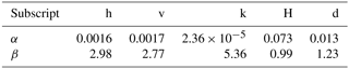
The values of the coefficients α_h, α_v, α_k, α_H, and α_d and β_h, β_v, β_k, β_H, and β_d for C-band in these equations are listed in Table 1. Hereafter, this converter is called FIT.

FIT is also applicable for X- and S-bands by replacing the coefficients. Although we already prepared the coefficients for all bands in the source codes, the users should carefully investigate their validity.

2.1.2 Observations of polarimetric parameters to model variables (KD)

The second converter (hereafter KD) converts observed K_DP to rainwater content (Q_rain) according to the following relation:

$$\begin{array}{}\text{(19)}& {\displaystyle }{Q}_{\mathrm{rain}}=\mathrm{3.565}{\left({\displaystyle \frac{K_{\mathrm{DP}}}{f}}\right)}^{\mathrm{0.77}},\end{array}$$

where f (GHz) is the radar frequency and the power-law coefficients are from Bringi and Chandrasekar (2001). Q_rain in the model is defined as Q_rain=Q_rρ_a (kg m⁻³). Note that Eq. (19) is applicable not only for C-band but also X- and S-bands by putting their frequencies in f. Equations (4)–(19) follow Kawabata et al. (2018), and we put the equations with different order in this paper for reader convenience to understand the flow of implementations of the forward, tangent linear, and adjoint codes.

Table 1 Values of the coefficients α and β. ${\mathit{\alpha }}_{\mathrm{h},\mathrm{v},\mathrm{k}}$ and ${\mathit{\beta }}_{\mathrm{h},\mathrm{v},\mathrm{k}}$ in Eqs. (9) and (10) and α_H,d in Eqs. (17) and (18) are from Kawabata et al. (2018), and β_H,d in Eqs. (17) and (18) is from Bringi and Chandrasekar (2001).

2.2 Tangent linear and adjoint operators

2.2.1 Tangent linear and adjoint operators of FIT

Because only p, T, and q_v are perturbed in WRF Var and NHM-4DVAR, the linearized form of Eq. (6) is

$$\begin{array}{ll}{\displaystyle }& {\displaystyle }\mathrm{\Delta }{\mathit{\rho }}_{\mathrm{a}}={\displaystyle \frac{\mathrm{\Delta }p}{RT\left(\mathrm{1}+\mathrm{0.61}{q}_{\mathrm{v}}\right)}}-{\displaystyle \frac{p\mathrm{\Delta }T}{R{T}^{\mathrm{2}}\left(\mathrm{1}+\mathrm{0.61}{q}_{\mathrm{v}}\right)}}\\ \text{(20)}& {\displaystyle }& {\displaystyle }-{\displaystyle \frac{\mathrm{0.61}p\mathrm{\Delta }{q}_{\mathrm{v}}}{RT{\left(\mathrm{1}+\mathrm{0.61}{q}_{\mathrm{v}}\right)}^{\mathrm{2}}}},\end{array}$$

and the perturbations of Λ and N₀ are given as

$$\begin{array}{}\text{(21)}& {\displaystyle }& {\displaystyle }\mathrm{\Delta }\mathrm{\Lambda }={\displaystyle \frac{\mathrm{1}}{\mathrm{3}}}\mathrm{\Lambda }\left(-\mathrm{\Delta }{Q}_{\mathrm{r}}{Q}_{\mathrm{r}}^{-\mathrm{1}}-\mathrm{\Delta }{\mathit{\rho }}_{\mathrm{a}}{\mathit{\rho }}_{\mathrm{a}}^{-\mathrm{1}}\right),\text{(22)}& {\displaystyle }& {\displaystyle }\mathrm{\Delta }{N}_{\mathrm{0}}=N_{\mathrm{r}}\mathrm{\Delta }\mathrm{\Lambda },\end{array}$$

where ΔQ_r and ΔN₀ are perturbations of the mixing ratio and number density of rainwater, respectively. Note that the perturbation of N_r is not considered in the adjoint model (see Sect. 2). Thus, the perturbations of Z_H,V, Z_DR, and K_DP are represented as follows.

$$\begin{array}{ll}{\displaystyle }& {\displaystyle }\mathrm{\Delta }{Z}_{\mathrm{H},\mathrm{V}}={\displaystyle \frac{\mathrm{4}{\mathit{\lambda }}^{\mathrm{4}}}{{\mathit{\pi }}^{\mathrm{4}}{\left|K_{\mathrm{w}}\right|}^{\mathrm{2}}}}\left({\mathit{\alpha }}_{\mathrm{h},\mathrm{v}}^{\mathrm{2}}\mathrm{\Gamma }\left(\mathrm{2}{\mathit{\beta }}_{\mathrm{h},\mathrm{v}}+\mathrm{1}\right)\left(\mathrm{\Delta }{N}_{\mathrm{0}}{\mathrm{\Lambda }}^{-\left(\mathrm{2}{\mathit{\beta }}_{\mathrm{h},\mathrm{v}}+\mathrm{1}\right)}\right.\right.\\ \text{(23)}& {\displaystyle }& {\displaystyle }\left.\left.-\left(\mathrm{2}{\mathit{\beta }}_{\mathrm{h},\mathrm{v}}+\mathrm{1}\right)\mathrm{\Delta }\mathrm{\Lambda }{N}_{\mathrm{0}}{\mathrm{\Lambda }}^{-\left(\mathrm{2}{\mathit{\beta }}_{\mathrm{h},\mathrm{v}}+\mathrm{2}\right)}\right)\right)\text{(24)}& {\displaystyle }& {\displaystyle }\mathrm{\Delta }{Z}_{\mathrm{DR}}=\mathrm{\Delta }{Z}_{\mathrm{h}}-\mathrm{\Delta }{Z}_{\mathrm{v}}{\displaystyle }& {\displaystyle }\mathrm{\Delta }{K}_{\mathrm{DP}}={\displaystyle \frac{\mathrm{180}\mathit{\lambda }}{\mathit{\pi }}}{\mathit{\alpha }}_{\mathrm{k}}\mathrm{\Gamma }\left({\mathit{\beta }}_{\mathrm{k}}+\mathrm{1}\right)\left(\mathrm{\Delta }{N}_{\mathrm{0}}{\mathrm{\Lambda }}^{-\left({\mathit{\beta }}_{\mathrm{k}}+\mathrm{1}\right)}\right.\\ \text{(25)}& {\displaystyle }& {\displaystyle }\left.-\left({\mathit{\beta }}_{\mathrm{k}}+\mathrm{1}\right)\mathrm{\Delta }\mathrm{\Lambda }{N}_{\mathrm{0}}{\mathrm{\Lambda }}^{-\left({\mathit{\beta }}_{\mathrm{k}}+\mathrm{2}\right)}\right)\end{array}$$

Finally, the perturbations of A_H and A_DP are

$$\begin{array}{}\text{(26)}& {\displaystyle }& {\displaystyle }\mathrm{\Delta }{A}_{\mathrm{H}}={\mathit{\alpha }}_{\mathrm{H}}{\mathit{\beta }}_{\mathrm{H}}\mathrm{\Delta }{K}_{\mathrm{DP}}{K_{\mathrm{DP}}}^{{\mathit{\beta }}_{\mathrm{H}}-\mathrm{1}},\text{(27)}& {\displaystyle }& {\displaystyle }\mathrm{\Delta }{A}_{\mathrm{DP}}={\mathit{\alpha }}_{\mathrm{d}}{\mathit{\beta }}_{\mathrm{d}}\mathrm{\Delta }{K}_{\mathrm{DP}}{K_{\mathrm{DP}}}^{{\mathit{\beta }}_{\mathrm{d}}-\mathrm{1}}.\end{array}$$

The adjoint operators are represented by the transposed form of Eqs. (20)–(27), which is (tangent linear)^T. As an example, the adjoint of Eq. (27) is

$$\begin{array}{}\text{(28)}& \mathrm{\Delta }{K}_{\mathrm{DP}}=\mathrm{\Delta }{K}_{\mathrm{DP}}+{\mathit{\alpha }}_{\mathrm{d}}{\mathit{\beta }}_{\mathrm{d}}{K_{\mathrm{DP}}}^{{\mathit{\beta }}_{\mathrm{d}}-\mathrm{1}}\mathrm{\Delta }{A}_{\mathrm{DP}}.\end{array}$$

2.2.2 Tangent linear and adjoint operators of KD

Because K_DP in Eq. (19) is an observed value, it is not necessary to linearize the equation. However, the equation that relates Q_rain to Q_r (Sect. 2.1.2) needs to be linearized as follows:

$$\begin{array}{}\text{(29)}& \mathrm{\Delta }{Q}_{\mathrm{rain}}=\mathrm{\Delta }{Q}_{\mathrm{r}}{\mathit{\rho }}_{\mathrm{a}}+Q_{\mathrm{r}}\mathrm{\Delta }{\mathit{\rho }}_{\mathrm{a}}.\end{array}$$

The transposed form of this equation is used for the adjoint model (see Sect. 2.2.1).

2.3 Space interpolator

Space interpolators in data assimilation systems map the model space to the observational space according to the representativeness of the observations. In the case of radar data, the effect of beam broadening stands for the representativeness, typically for a beam width of approximately 1.0^∘. The broadening is characterized by a Gaussian distribution orthogonal to the direction of the radar beam. Most previous studies (e.g., Seko et al., 2004; Wattrelot et al., 2014), except Zeng et al. (2016), consider only vertical beam broadening because numerical models have horizontal grid spacings of several kilometers, whereas they have vertical grid spacings in the lower troposphere of less than 1 km. However, data assimilation systems must have sub-kilometer horizontal grid spacings as well (e.g., Kawabata et al., 2014a; Miyoshi et al., 2016) so that the space interpolators can take account of horizontal beam broadening. In addition, several phased-array radars recently deployed in Japan have different beam widths in the vertical and horizontal directions. Our operator thus considers beam broadening in both the vertical and horizontal directions.

In addition, it is important for the space interpolator to include beam-bending effects, which depend on atmospheric conditions. In this study, the bending is determined by considering the climatological vertical gradient of the refractive index of the atmosphere in accordance with the effective Earth radius model (Doviak and Zrnić, 1993) following Haase and Crewell (2000), who showed statistically that the climatological refractive index is close to the actual refractive index at elevation angles higher than 1^∘ instead of by considering the actual atmospheric conditions, although Zeng et al. (2014) developed an excellent radar simulator that considers the actual refractivity of the atmosphere.

Remote sensing observations usually have higher spatial resolutions than model grid spacings. To avoid correlations of the observational errors in such high-resolution data, it is necessary either to thin the data or to use “super observations”. In this study, we chose the super observation method, in which observations are averaged over each model grid cell. Super observation methods also have the advantage that they remove undesirable fluctuations associated with sub-grid-scale phenomena, the assimilation of which makes the numerical model unnecessarily noisy (e.g., Seko et al., 2004; Zhang et al., 2009).

First, we calculated the path of the center of the radar beam in the model domain, including its elevation, azimuth, and bending angles (Fig. 1a). Once sufficient data are included within a model grid cell, they are averaged and mapped onto an interpolation point along the radar beam (IP in Fig. 1). This value at this point is a “super observation”, and it is compared with the modeled value, which was interpolated by using Gaussian weights (Fig. 1b). Moreover, we also developed the tangent and adjoint codes of the space interpolator.

3 Setup options

The operators are controlled by the namelist (“namelist.polradar”) as follows.

&name_obs o_dir='/home/usr/datadir', o_stn(1)='OFT', o_stn(2)='TUR', icnv=0/

Here, “o_dir” is the directory for the input observational data, “o_stn” indicates the station names of radar sites, where “max_stn”, the number of names, is set in “da_setup_obs_structures_polradar.inc” in WRF Var and in “obs_dual_pol.f90:” in NHM-4DVAR, and “icnv” is a switch for the selection of the observational operator, where “0” and “5” mean FIT and KD, respectively.

In addition, a file that defines for each radar area where the beam is blocked by topography, named “beam_block_rate_${radar_site}.dat”, must be supplied by the user. This file is made by another program and should be prepared before the assimilation.

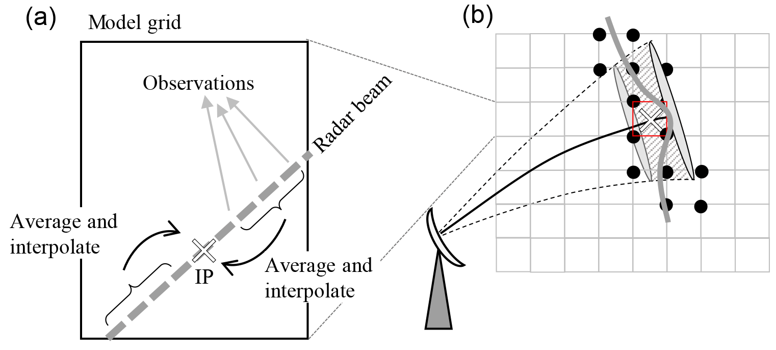
Figure 1 Schematic diagrams of (a) a super observation and (b) the space interpolator. Boxes represent model grid cells, and the red box indicates the grid cell in which the super observation is defined. The cross marks represent the interpolation point (IP). In panel (b), the grey curve indicates the Gaussian weights at various grid points (black circles), the solid black line shows the beam propagation, and the dashed lines illustrate beam broadening.

4 Results

4.1 Verification of the tangent linear and adjoint operators of FIT

In this section, we examine the linearity of only the FIT variable converter; it is not necessary to examine the linearity of the KD converter because of the intrinsic linearity of Eq. (19). We evaluated the linearity of FIT by performing a Taylor expansion. If the original equation is given as

$$\begin{array}{}\text{(30)}& \mathbf{y}=H\left(\mathbf{x}\right),\end{array}$$

then the linearized equation is defined as

$$\begin{array}{}\text{(31)}& \mathit{\delta }\mathbf{y}=\mathbf{H}\mathit{\delta }\mathbf{x}.\end{array}$$

If the linear equation is derived with no errors, the following Taylor expansion of Eq. (31),

$$\begin{array}{}\text{(32)}& {\displaystyle \frac{\mathrm{|}H\left(\mathbf{x}+\mathit{\alpha }\mathit{\delta }\mathbf{x}\right)-H\left(\mathbf{x}\right)\mathrm{|}}{\left|\mathit{\alpha }\right|\mathrm{|}\mathbf{H}\mathit{\delta }\mathbf{x}\mathrm{|}}}=\mathrm{1}+O\left(\mathit{\alpha }\right),\end{array}$$

should be accurate within the rounding error of the computer. The results for Z_H, Z_V, and K_DP in Eqs. (11) and (14) are 1.00 when α is 10⁻⁷ to 10⁻¹⁵.

Regarding the adjoint operator, we evaluated the following equation:

$$\begin{array}{}\text{(33)}& {\left(\mathbf{H}\mathit{\delta }\mathbf{x}\right)}^{\mathrm{T}}\left(\mathbf{H}\mathit{\delta }\mathbf{x}\right)=\mathit{\delta }{\mathbf{x}}^{\mathrm{T}}\left[{\mathbf{H}}^{\mathrm{T}}\left(\mathbf{H}\mathit{\delta }\mathbf{x}\right)\right],\end{array}$$

where the left-hand side of Eq. (33) is calculated using the tangent linear operator, and on the right-hand side, the output variables of the tangent linear operator are input into the adjoint operator. This equation must be accurate within the rounding error. In FIT, the difference between the left- and right-hand sides was −8.215650382 × 10⁻¹⁵, which we consider accurate enough.

4.2 Actual data assimilation test

We conducted two simple data assimilation tests. Observational errors of Z_h, Z_DR, K_DP, and Q_rain, which were determined after the statistical examination (Kawabata et al., 2018), were 15.0 dBZ, which is the same as in Kawabata et al. (2011) at 2.0 dB, 4.0^∘ km⁻¹, and 4 g m⁻³, respectively. These errors are homogeneous in space, which means observational error covariances are diagonal.

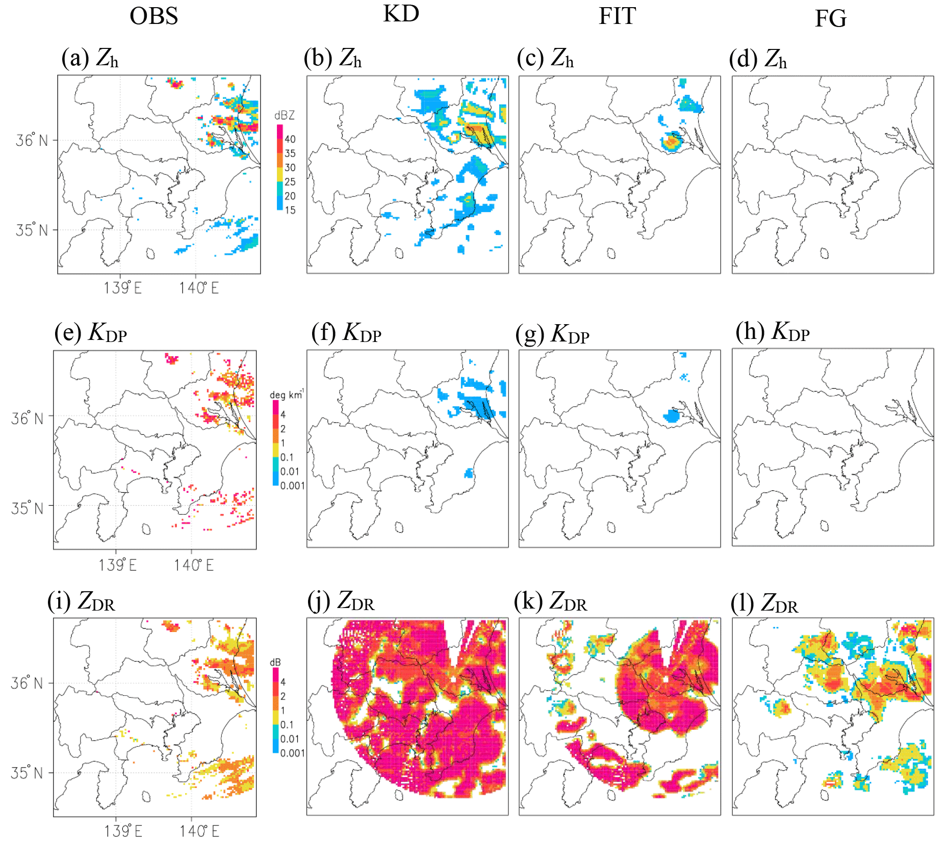
Figure 2 From left to right, horizontal distributions of polarimetric parameters of observations (OBS), assimilation results by KD and FIT with NHM-4DVAR, and the first-guess field (FG) at 21:04 UTC on 23 June 2014. (a–d) Z_h; (e–h) K_DP; (i–l) Z_DR.

The first one was done using NHM-4DVAR with actual radar data from the C-band dual polarimetric radar at the Meteorological Research Institute in Tsukuba, Japan (Yamauchi et al., 2012; Adachi et al., 2013). In this experiment, both radial velocity data and the polarimetric parameters of Z_H, Z_DR, and K_DP were assimilated in FIT, and radial velocity and Q_rain derived from K_DP were assimilated in KD. The assimilation window was from 21:00 to 21:05 UTC on 23 June 2014, a day on which intense hail fell in Tokyo, Japan. The horizontal resolution of NHM-4DVAR was 2 km and the length of the assimilation window was 5 min, 11 PPI data from 0.5 to 4.8^∘ elevations with the azimuth resolution of 0.7^∘ and the range resolution of 150 m were assimilated. PPI data were assimilated at the exact observation time as far as the time interval of NHM-4DVAR (10 s in this case) permits. The background errors were described in Kawabata et al. (2007, 2011). Analysis (KD and FIT) and observational (OBS) fields of Z_h, Z_DR, andK_DP are shown in Fig. 2, which displays the whole assimilation domain. Although there was no rain region in the first-guess field (FG; Fig. 2d), Z_h in KD was comparable to that in OBS from the standpoint of rainfall distribution and intensity, but Z_h in FIT covered a much smaller area than it did in OBS. This smaller coverage may be due to nonlinearity in FIT. In KD, we can see quite small values of K_DP (Fig. 2f), but good agreement with OBS in its horizontal distribution, while Z_h looks better than K_DP. K_DP values were smaller in both KD and FIT than in OBS. This result is similar to that of a statistical analysis performed by Kawabata et al. (2018). In contrast, Z_DR values in KD and FIT were larger than OBS over large areas. This result implies that the calculation of the axis ratio of raindrops (Eq. 8) may need modification because in the FG field, Z_DR values and coverage were already too large in comparison with those of OBS.

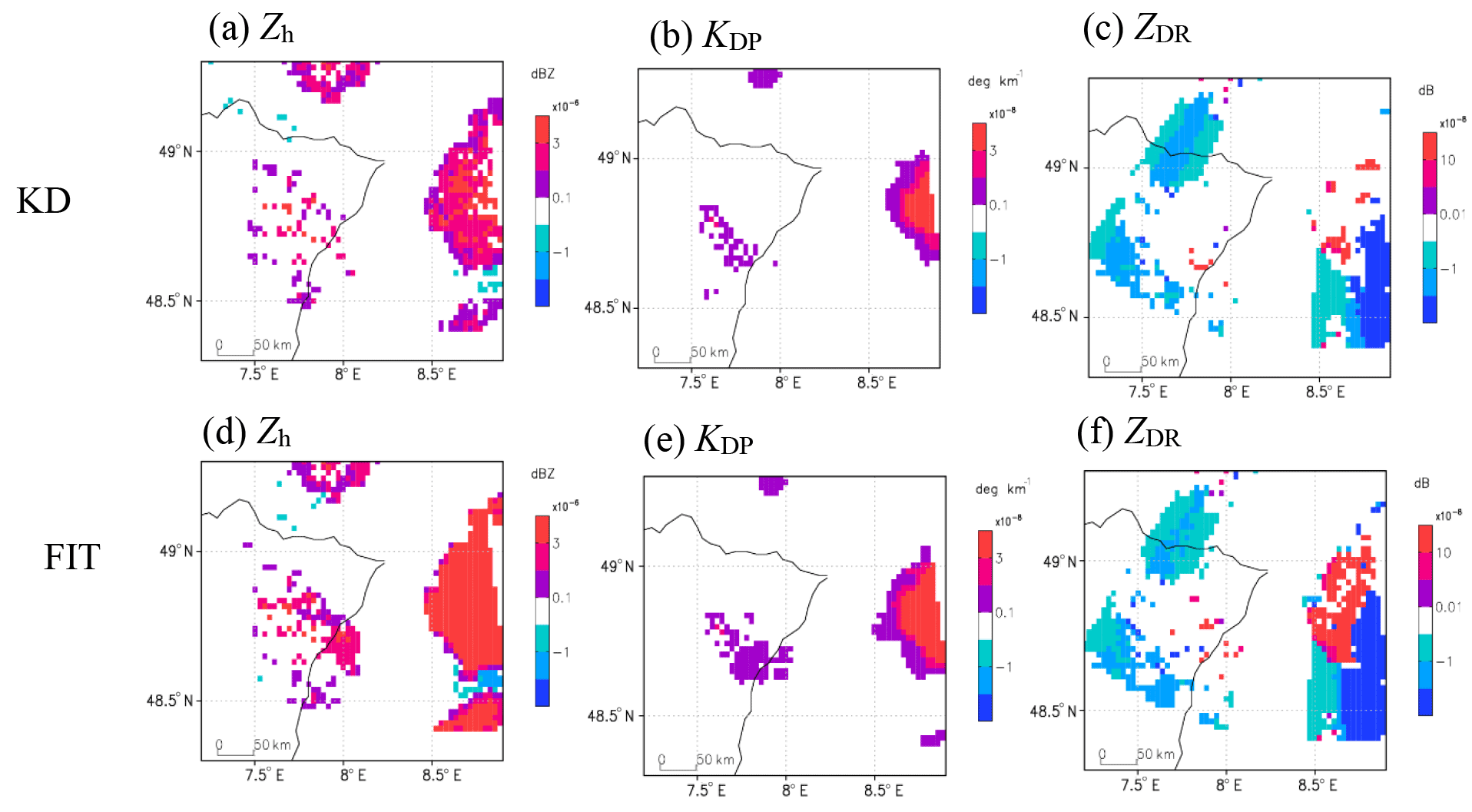
Figure 3 Horizontal distributions of differences in polarimetric parameters between assimilation results by KD and FIT with WRF 3D-Var and observations at 11:00 UTC on 14 August 2014.

The second one was done using WRF 3D-Var with actual radar data from the DWD radar network (Helmert et al., 2014) for the same case with “Case 1” described in Kawabata et al. (2018). The horizontal resolution of WRF 3D-Var was 2 km, and polarimetric parameters and rainwater content in single PPI data by Offenthal radar were assimilated (see Kawabata et al., 2018, for detailed information on the observation). The background errors were calculated with ensemble simulations by WRF initialized by ECMWF analysis using the “gen_be” tool compiled in WRFDA. Observational errors were the same as the first case. From the increments of polarimetric parameters (Fig. 3), although quite small impacts are seen, similar patterns are recognized in both methods and larger impacts of Z_h and Z_DR were produced in FIT and KD, respectively.

In both cases, the radial velocity data were assimilated with the same method as in Sun and Crook (1997).

5 Summary

We implemented two variable converters for polarimetric radars in the WRF variational data assimilation system (WRF Var) and the JMANHM data assimilation system (NHM-4DVAR). FIT simulates polarimetric parameters using a double-moment cloud microphysics scheme, and KD estimates rainwater contents with the observed specific differential phase. Both FIT and KD are applicable not only for C-band but also X- and S-bands. The advantage of FIT over KD is that it includes theoretically precise formulations for both the mixing ratio and number density of rainwater, as well as attenuation effects, whereas KD has advantages due to its linear formulation and small computational cost.

These operators work in conjunction with an advanced space interpolator, which considers (1) beam broadening in three dimensions, (2) different beam widths in the vertical and horizontal directions, and (3) the climatological beam-bending effect. The interpolator also simulated attenuation effects.

Tangent and adjoint operators of the two variable converters and the space interpolator were developed and implemented along with the forward operators. In a simple data assimilation experiment, we succeeded in assimilating actual polarimetric observations and obtained reasonable results with both the FIT and KD operators, except for Z_DR. However, our results show a need for further improvements of the K_DP and Z_DR estimates. It would be possible to overcome the weaknesses of the Z_h distributions in FIT and FG through assimilation–forecast cycles and/or by adding other types of observation data, such as conventional observations, Doppler (water vapor) lidar data, and water vapor data observed by GNSS. Furthermore, it is necessary to improve quality controls (QCs) for polarimetric parameters, although the same QCs were applied as described in Kawabata et al. (2018) and the impact of axis ratio (Eq. 8) and observational errors on assimilations will be investigated, and it is necessary to estimate more appropriate observational errors (e.g., Wulfmeyer et al., 2016). These challenges would improve QPE and QPF with the current forms of the operators.