FAIR v1.3: a simple emissions-based impulse response and carbon cycle model

Simple climate models can be valuable if they are able to replicate aspects of complex fully coupled earth system models. Larger ensembles can be produced, enabling a probabilistic view of future climate change. A simple emissions-based climate model, FAIR, is presented, which calculates atmospheric concentrations of greenhouse gases and effective radiative forcing (ERF) from greenhouse gases, aerosols, ozone and other agents. Model runs are constrained to observed temperature change from 1880 to 2016 and produce a range of future projections under the Representative Concentration Pathway (RCP) scenarios. The constrained estimates of equilibrium climate sensitivity (ECS), transient climate response (TCR) and transient climate response to cumulative CO₂ emissions (TCRE) are 2.86 (2.01 to 4.22) K, 1.53 (1.05 to 2.41) K and 1.40 (0.96 to 2.23) K (1000 GtC)⁻¹ (median and 5–95 % credible intervals). These are in good agreement with the likely Intergovernmental Panel on Climate Change (IPCC) Fifth Assessment Report (AR5) range, noting that AR5 estimates were derived from a combination of climate models, observations and expert judgement. The ranges of future projections of temperature and ranges of estimates of ECS, TCR and TCRE are somewhat sensitive to the prior distributions of ECS∕TCR parameters but less sensitive to the ERF from a doubling of CO₂ or the observational temperature dataset used to constrain the ensemble. Taking these sensitivities into account, there is no evidence to suggest that the median and credible range of observationally constrained TCR or ECS differ from climate model-derived estimates. The range of temperature projections under RCP8.5 for 2081–2100 in the constrained FAIR model ensemble is lower than the emissions-based estimate reported in AR5 by half a degree, owing to differences in forcing assumptions and ECS∕TCR distributions.

1 Introduction

Most multi-model studies, such as the Coupled Model Intercomparison Project (CMIP), which produces headline climate projections for the Intergovernmental Panel on Climate Change (IPCC) assessment reports, compare atmosphere–ocean general circulation models that are run with prescribed concentrations of greenhouse gases. Greenhouse gas and aerosol emissions time series are provided by integrated assessment modelling groups based on socio-economic narratives (Moss et al., 2010; Meinshausen et al., 2011b), which are then converted to atmospheric concentrations by simple climate–carbon-cycle models such as MAGICC6 (Meinshausen et al., 2011a). Earth system models can be run in emissions mode, where emissions of carbon dioxide are used as a starting point and the atmospheric CO₂ concentrations are calculated interactively in the model, with atmospheric concentration changes being the residual of emissions minus absorption by land and ocean sinks. While many models include the functionality to be run in CO₂ emissions-driven mode, these integrations were not the main focus of CMIP5 (the fifth phase of CMIP; Taylor et al., 2012).

Earth system models in CMIP5 all show a positive carbon cycle feedback, meaning that as surface temperature increases, land and ocean carbon sinks become less effective at absorbing CO₂ and a larger proportion of any further emitted carbon will remain in the atmosphere (Friedlingstein, 2015). The various feedback strengths are nevertheless model dependent (Friedlingstein et al., 2006). While CO₂ is the most important climate forcer, individual models may also differ in their responses to non-CO₂ emissions. These emissions can also introduce uncertainty that is not captured in concentration-driven or CO₂-only driven model experiments (Matthews and Zickfeld, 2012; Tachiiri et al., 2015; Gasser et al., 2017). As non-CO₂ forcing impacts temperature, which affects the efficiency of carbon sinks, non-CO₂ forcing agents themselves influence the carbon cycle (MacDougall et al., 2015; Tokarska et al., 2018).

Simple models can be used to emulate radiative forcing and temperature responses to emissions and atmospheric concentrations and can be tuned to replicate the behaviour of individual climate and earth system models (Meinshausen et al., 2011a; Good et al., 2011, 2013; Geoffroy et al., 2013). A simple emulation of the carbon cycle of full- and intermediate-complexity earth system models was developed by Joos et al. (2013) and used in the IPCC Fifth Assessment Report (AR5) for the purposes of calculating global warming potentials. The model was developed for a 100  GtC pulse against a background CO₂ concentration of 389 ppm. Millar et al. (2017) showed that this model does not sufficiently capture the time-evolving dependency of carbon sinks against different background conditions. They introduced the Finite Amplitude Impulse Response (FAIR) model (version 1.0) that tracks the time-integrated airborne fraction of carbon and uses this to determine the efficiency of carbon sinks, in turn calculating atmospheric CO₂ concentrations, radiative forcing and temperature change.

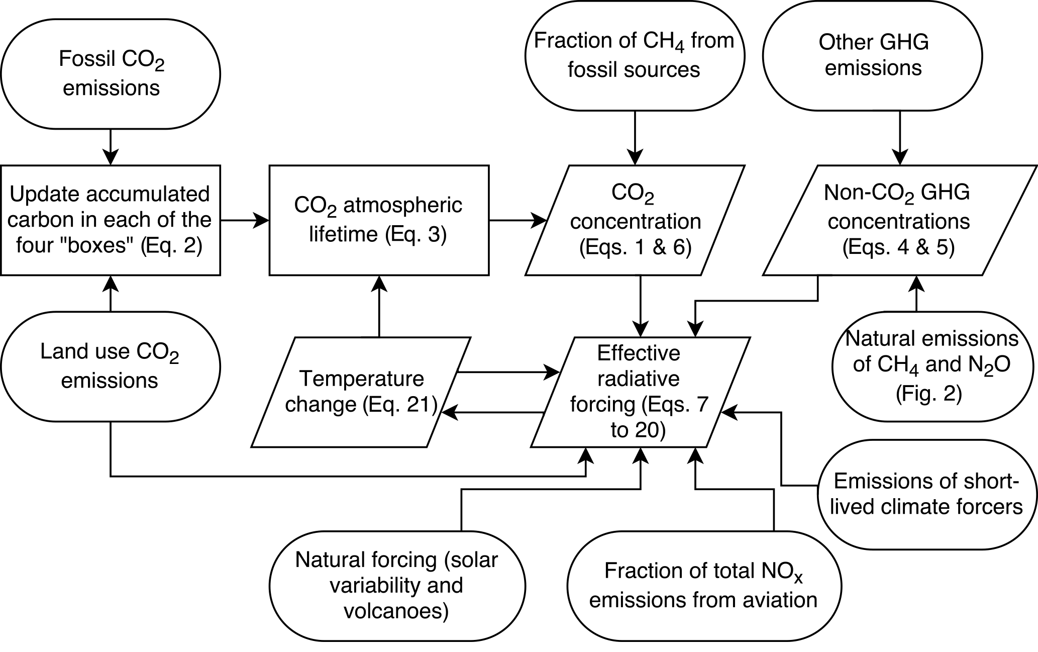
FAIR v1.0 is well-calibrated to the temperature and carbon cycle response of earth system models. FAIR v1.3 is extended to calculate non-CO₂ greenhouse gas concentrations from emissions, aerosol forcing from aerosol precursor emissions, tropospheric and stratospheric ozone forcing from the emissions of precursors, and forcings from black carbon on snow, stratospheric methane oxidation to water vapour, contrails and land use change. Forcings from volcanic eruptions and solar irradiance fluctuations are supplied externally. These forcings are then converted to a temperature change, taking into account the different thermal responses of the ocean mixed layer and deep ocean.

The model philosophy in FAIR is to represent these processes as simply as possible and to be able to emulate the historical effective radiative forcing (ERF) time series in AR5 given input emissions. FAIR is written in Python and is open source. The extension to non-CO₂ emissions makes FAIR v1.3 applicable for assessing scenarios with a broad range of emissions pathways.

This paper introduces the FAIR model in Sect. 2, including the key changes from versions 1.0 to 1.3. Section 3 then discusses the generation of a large ensemble of input parameters to the FAIR model which is run and results described in Sect. 4. A sensitivity analysis to some of the key inputs to the large ensemble is given in Sect. 5. Section 6 provides a summary.

2 Development of FAIR v1.3 and differences to v1.0

FAIR v1.3 takes emissions of greenhouse gases and short-lived climate forcers as its main input. This is an array of size (number of years × 40) (see Table 1) and is based on the order provided in the Representative Concentration Pathway (RCP) emissions datasets (Meinshausen et al., 2011b). Additional options that can be specified by the user include the treatment of aviation contrail and land use forcing, the fraction of total methane attributable to fossil fuels, natural emissions of CH₄ and N₂O, and natural forcing from solar variability and volcanoes. The atmospheric concentrations of greenhouse gases are calculated from new emissions minus the decay of the current atmospheric burden, which is determined by the atmospheric lifetime of each gas, and output is produced as a (years × 31) array (Table 2). For CO₂, atmospheric concentrations are calculated from a simple representation of the carbon cycle which includes temperature and saturation dependency of land and ocean sinks. The calculated CO₂ concentrations at each timestep also include a proportion of methane oxidised to CO₂. This is on the assumption of a mole of oxidised methane from fossil sources is not also counted as a mole of CO₂ when reported in national emissions inventories (Gillenwater, 2008; Boucher et al., 2009).

The effective radiative forcing (ERF) from 13 different forcing agents (Table 3) is determined from the concentrations of each greenhouse gas, plus emissions of short-lived climate forcers and natural forcing, and is output from the model as a (years × 13) array. From the ERF, temperature change is calculated. The change in temperature feeds back into the carbon cycle, which impacts the atmospheric lifetime of carbon dioxide. A flow diagram outlining the key processes is provided in Fig. 1. It is also possible to run FAIR using only CO₂ emissions as inputs or purely in forcing-only mode, where a time series of non-CO₂ or total forcing can be optionally specified rather than calculated from emissions.

Table 1 Emissions time series input used in FAIR, based on the RCP emissions datasets in Meinshausen et al. (2011b).

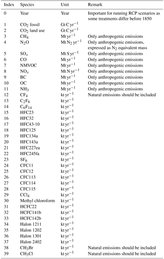
Table 2 The set of greenhouse gases used in FAIR. With the exception of methane lifetime, radiative efficiencies and lifetimes are from AR5 (Myhre et al., 2013b, Table 8.A.1). For ozone-depleting substances, the fractional release coefficients r_i (Daniel and Velders, 2011) and the number of chlorine and bromine atoms are also given for the calculation of equivalent effective stratospheric chlorine (Eq. 14). Where ERF is not calculated as a linear function of concentration, “not applicable” (N/A) is displayed.

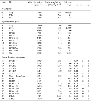
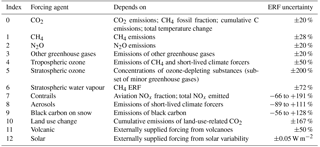
Table 3 The 13 separate forcing groups considered in FAIR v1.3 in the calculation of effective radiative forcing. The ERF uncertainty represents the 5–95 % range and is used in the generation of the large ensemble (Sect. 3). ERF uncertainties from Myhre et al. (2013b) are used except for CH₄ where we use the Myhre et al. (2013b) estimate inflated by the additional uncertainty in the new methane forcing relationship in Etminan et al. (2016), which also affects the uncertainty in stratospheric water vapour oxidation from methane.

Figure 1 Simplified overview of the FAIR v1.3 model.

2.1 Greenhouse gases: emissions to concentrations

2.1.1 Carbon dioxide and carbon cycle

The carbon cycle component in FAIR is described in detail by Millar et al. (2017) and an overview is provided here. The FAIR model uses anthropogenic fossil and land use CO₂ emissions as input and partitions them into four boxes R_i (with partition fraction a_i and ${\sum }_{\mathrm{0}}^{\mathrm{3}}{a}_i=\mathrm{1}$) representing the differing timescales of carbon uptake by geological processes (τ₀), the deep ocean (τ₁), the biosphere (τ₂) and the ocean mixed layer (τ₃). The atmospheric molar mixing ratio of CO₂ and its relationship to each box is

$$\begin{array}{}\text{(1)}& C_{{\text{CO}}_{\mathrm{2}}}=C_{{\text{CO}}_{\mathrm{2}},\text{pi}}+\sum _{i=\mathrm{0}}^{\mathrm{3}}{\displaystyle \frac{R_i}{M_{\text{a}}}}{\displaystyle \frac{w_{{\text{CO}}_{\mathrm{2}}}}{w_{\text{a}}}},\end{array}$$

with $C_{{\text{CO}}_{\mathrm{2}},\text{pi}}$ equal to 278 ppm and the subscript pi representing a pre-industrial state. $M_{\text{a}}=\mathrm{5.1352}\times {\mathrm{10}}^{\mathrm{18}}$ kg is the dry mass of the atmosphere, and $w_{{\mathrm{CO}}_{\mathrm{2}}}$ and w_a are the molecular weights of CO₂ and dry air. R_i is in kilograms. The governing equations for the four boxes are

$$\begin{array}{}\text{(2)}& {\displaystyle \frac{\text{d}{R}_i}{\text{d}t}}=a_i{E}_{{\text{CO}}_{\mathrm{2}}}-{\displaystyle \frac{R_i}{\mathit{\alpha }{\mathit{\tau }}_i}};i=\mathrm{0},\mathrm{\dots },\mathrm{3},\end{array}$$

with $E_{{\text{CO}}_{\mathrm{2}}}$ being the emissions of CO₂.

The four time constants τ_i are scaled by a factor α depending on the 100-year integrated impulse response function (iIRF₁₀₀), which represents the 100-year average airborne fraction of a pulse of CO₂ (Joos et al., 2013). α is found by equating two different expressions for iIRF₁₀₀

$$\begin{array}{}\text{(3)}& \sum _{i=\mathrm{0}}^{\mathrm{3}}\mathit{\alpha }{a}_i{\mathit{\tau }}_i\left[\mathrm{1}-\exp \left({\displaystyle \frac{-\mathrm{100}}{\mathit{\alpha }{\mathit{\tau }}_i}}\right)\right]=r_{\mathrm{0}}+r_{\text{C}}{C}_{\text{acc}}+r_{\text{T}}T\end{array}$$

and finding the unique root α (Millar et al., 2017). The right-hand side of Eq. (3) proposed by Millar et al. (2017) is a simplified expression for iIRF₁₀₀ that depends on the total accumulated carbon in land and ocean sinks $C_{\text{acc}}=\left({\sum }_t{E}_{{\text{CO}}_{\mathrm{2}},t}\right)-(C_{{\text{CO}}_{\mathrm{2}}}-C_{{\text{CO}}_{\mathrm{2}},\text{pi}})$ and temperature change T since the pre-industrial era that simulates the behaviour of earth system models well. This increase in iIRF₁₀₀ and scaling of the time constants by α accounts for the land and ocean carbon sinks changing absorption efficacy as more carbon is added to them (r_C parameter). In earth system models it is also observed that the efficiency of carbon sinks decreases with increasing temperature (r_T parameter; Fung et al., 2005; Friedlingstein et al., 2006). Following Millar et al. (2017) we use r_C=0.019 yr GtC⁻¹ and r_T=4.165 yr K⁻¹, but in contrast to Millar et al. (2017) a pre-industrial r₀=35 years is used rather than their 32.4 years. This facilitates better agreement with present-day CO₂ atmospheric concentrations when spun up from 1765 with historical CO₂ and non-CO₂ emissions. This parameter combination is consistent with a present-day iIRF₁₀₀ diagnosed from more complex carbon cycle models (Joos et al., 2013) with a fixed background CO₂ concentration of 389 ppm.

2.1.2 Other greenhouse gases

A one-box decay model is assumed for other greenhouse gases where the sink is an exponential decay of the existing gas concentration anomaly. New emissions are converted to the equivalent increase in molar mixing ratios δC in year t by

$$\begin{array}{}\text{(4)}& \mathit{\delta }{C}_t={\displaystyle \frac{E_t}{M_{\text{a}}}}{\displaystyle \frac{w_{\text{a}}}{w_{\text{f}}}}{\mathit{\delta }}_t,\end{array}$$

where E_t is the emissions of gas in year t, $M_{\text{a}}=\mathrm{5.1352}\times {\mathrm{10}}^{\mathrm{18}}$ kg is the mass of the atmosphere and w_f is the molecular mass of the greenhouse gas (δ_t=1 for annual emissions data). The model updates the atmospheric molar mixing ratios C at year t based on new emissions and the natural sink by

$$\begin{array}{}\text{(5)}& C_t=C_{t-\mathrm{1}}+{\displaystyle \frac{\mathrm{1}}{\mathrm{2}}}\left(\mathit{\delta }{C}_{t-\mathrm{1}}+\mathit{\delta }{C}_t\right)-C_{t-\mathrm{1}}\left(\mathrm{1}-\exp (-\mathrm{1}/\mathit{\tau })\right),\end{array}$$

where τ is the atmospheric lifetime of each gas (Table 2).

For CH₄ and N₂O, time-varying natural emissions are included in E_t (Fig. 2) in order to match the observed atmospheric concentrations of these gases in Meinshausen et al. (2011b), including the 1765 concentrations when the 1765 natural emissions are run to steady state. Beyond 2005, natural emissions of CH₄ and N₂O are fixed at 191 Mt CH₄ yr⁻¹ and 8.99 Mt N₂-eq yr⁻¹, which are close to the best-estimate present-day emissions of 202 Mt CH₄ yr⁻¹ and 9.1 Mt N₂-eq yr⁻¹ (Prather et al., 2012). We prefer to use varying natural emissions with a fixed atmospheric lifetime of CH₄ and N₂O, firstly because this provides a good match to observed and projected concentrations and secondly because this is consistent with the simple model philosophy. Other methods of calculating concentrations of these gases are possible, for example using a fixed natural background emission and relating any differences between observed and calculated historical concentrations as an error term (either in the natural or anthropogenic time series or missing processes) or by adjusting the atmospheric lifetime of each gas over the historical period in order to match the observed concentrations at each time step.

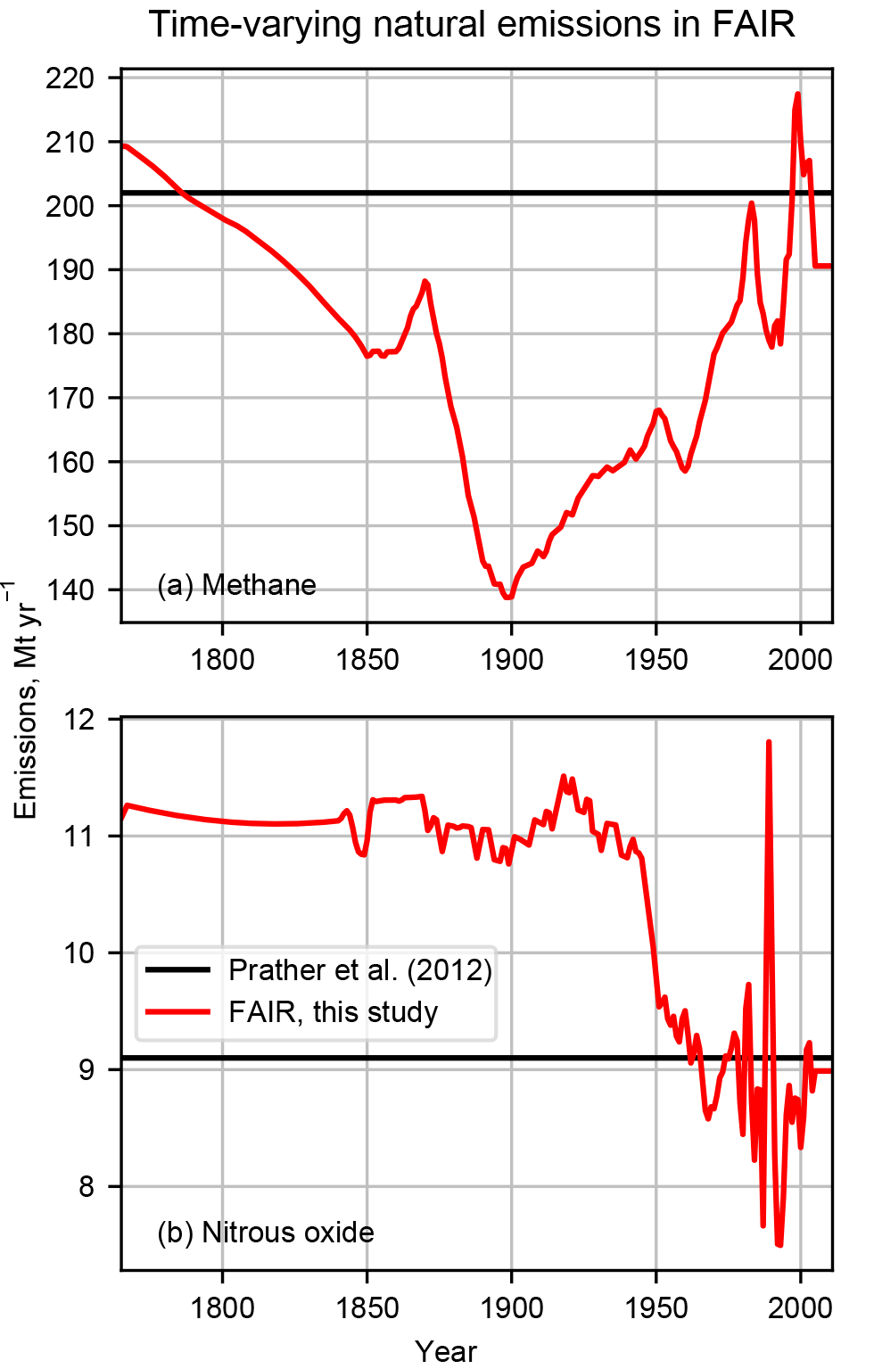
Figure 2 Natural emissions of methane and nitrous oxide used in the FAIR model. Future emissions are fixed at their 2011 values. Also shown are the present-day best estimates of Prather et al. (2012).

Natural emissions of CO₂ are not included as the carbon cycle model is more complex than the single box used for other gases and it is assumed that natural sources and natural sinks are in balance. For other greenhouse gases, natural emissions are assumed to be zero except for CF₄, CH₃Br and CH₃Cl. Pre-industrial concentrations of these three minor compounds are estimated by running the 1765 emissions from Meinshausen et al. (2011b) to steady state using the lifetimes in Table 2. Unlike CH₄ and N₂O, natural emissions of CF₄, CH₃Br and CH₃Cl are included in the anthropogenic emissions data. In total, 31 greenhouse gas species are used (Table 2). Other than CO₂, CH₄ and N₂O, the remaining gases can be subdivided into those covered by the Kyoto Protocol (HFCs, PFCs, SF₆) and the ozone-depleting substances (ODSs) covered by the Montreal Protocol (CFCs, HCFCs, and other chlorinated and brominated compounds).

The best estimate of τ for each gas except methane is used from AR5 (Myhre et al., 2013b, Table 8.A.1), consistent with using AR5 estimates for parameters where possible. We find that using a constant methane lifetime of 9.3 years results in reasonable levels of historical natural emissions and also agrees well with the MAGICC6-projected RCP concentration scenarios in the future. The global methane lifetime of 9.3 years used is significantly lower than the perturbation lifetime of 12.4 years in AR5. This latter figure includes the feedback of methane emissions on its own lifetime due to the depletion of the OH radical, which is the main tropospheric sink for methane (a factor of 1.34; Holmes et al., 2013, also used in AR5), and is used for perturbation calculations against a constant background concentration. As emissions of OH-affecting species (NO_x, non-methane volatile organic compounds (NMVOCs), CO) and temperature have varied substantially over the historical period, the background state is not constant, so the perturbation lifetime is not appropriate.

2.1.3 Methane oxidation to CO₂

The oxidation of CH₄ produces additional CO₂ if it is of fossil origin, which is accounted for in the model. Methane is assumed to be from fossil sources if it arises from the transport, energy or industry sectors. A best estimate of 61 % of the methane lost through reaction with the hydroxyl radical in the troposphere (the dominant loss pathway) is converted to CO₂ (Boucher et al., 2009). This is treated as additional emissions of CO₂:

$$\begin{array}{ll}{\displaystyle }{E}_{{\mathrm{CH}}_{\mathrm{4}}\to {\mathrm{CO}}_{\mathrm{2}}}& {\displaystyle }=\mathrm{0.61}{f}_{{\mathrm{CH}}_{\mathrm{4}}\text{fos}}\left(C_{{\mathrm{CH}}_{\mathrm{4}}}-C_{{\mathrm{CH}}_{\mathrm{4}},\text{pi}}\right)\\ \text{(6)}& {\displaystyle }& {\displaystyle }\left(\mathrm{1}-\exp (-\mathrm{1}/{\mathit{\tau }}_{{\mathrm{CH}}_{\mathrm{4}}})\right),\end{array}$$

where $f_{{\mathrm{CH}}_{\mathrm{4}}\text{fos}}$ is the fraction of anthropogenic methane attributable to fossil sources and ${\mathit{\tau }}_{{\mathrm{CH}}_{\mathrm{4}}}$ is 9.3 years. Both the fraction of methane converted (61 %) and the time series of the fraction of methane that is of fossil origin $f_{{\mathrm{CH}}_{\mathrm{4}}\text{fos}}$ are user-specifiable, and RCP-derived values available from the RCP Database (2009) can be imported. The user can therefore switch off methane oxidation by setting either of these values to zero.

Oxidation of CO and NMVOCs to CO₂ is not included as to not double count the carbon that is included in national CO₂ emissions inventories (Daniel and Solomon, 1998; Gillenwater, 2008).

2.2 Effective radiative forcing

The ERF from 13 different forcing agent groups are considered: CO₂, CH₄, N₂O, other greenhouse gases, tropospheric O₃, stratospheric O₃, stratospheric water vapour, contrails, aerosols, black carbon on snow, land use change, solar irradiance and volcanoes (Table 3). ERF, which accounts for all (stratospheric plus tropospheric) rapid adjustments, corresponds better to temperature change than “traditional” stratospherically adjusted radiative forcing (RF) (Myhre et al., 2013b; Forster et al., 2016). Therefore, we use relationships for ERF where they exist.

2.2.1 Carbon dioxide, methane and nitrous oxide

We use the updated Etminan et al. (2016) RF relationships for CO₂, CH₄ and N₂O, which for the first time includes band overlaps between CO₂ and N₂O. It also includes a significant upward revision of the CH₄ RF due to inclusion of previously neglected shortwave absorption, compared to the previous relationships of Myhre et al. (1998) used in AR5. Although Etminan et al. (2016) calculate RF, Myhre et al. (2013b) concluded that over the industrial era there was not sufficient evidence to state that ERF was significantly different from RF for these three gases, and ERF is taken to equal RF, although with a doubled uncertainty range. The Etminan et al. (2016) relationships are reproduced in Eqs. (7)–(9), where C (ppm), M and N (ppb) have been used to represent concentrations of CO₂, CH₄ and N₂O, and the subscript pi representing pre-industrial concentrations.

$$\begin{array}{ll}{\displaystyle }{F}_{{\mathrm{CO}}_{\mathrm{2}}}=& {\displaystyle }\left[(-\mathrm{2.4}\times {\mathrm{10}}^{-\mathrm{7}})(C-C_{\text{pi}}{)}^{\mathrm{2}}+(\mathrm{7.2}\times {\mathrm{10}}^{-\mathrm{4}})\right.\\ {\displaystyle }& {\displaystyle }\left.|C-C_{\text{pi}}|-(\mathrm{1.05}\times {\mathrm{10}}^{-\mathrm{4}})(N+N_{\text{pi}})+\mathrm{5.36}\right]\\ \text{(7)}& {\displaystyle }& {\displaystyle }\times \log \left({\displaystyle \frac{C}{C_{\text{pi}}}}\right),{\displaystyle }{F}_{{\mathrm{N}}_{\mathrm{2}}\mathrm{O}}=& {\displaystyle }\left[(-\mathrm{4.0}\times {\mathrm{10}}^{-\mathrm{6}})(C+C_{\text{pi}})+(\mathrm{2.1}\times {\mathrm{10}}^{-\mathrm{6}})\right.\\ {\displaystyle }& {\displaystyle }\left.(N+N_{\text{pi}})-(\mathrm{2.45}\times {\mathrm{10}}^{-\mathrm{6}})(M+M_{\text{pi}})+\mathrm{0.117}\right]\\ \text{(8)}& {\displaystyle }& {\displaystyle }\times \left(\sqrt{N}-\sqrt{N_{\text{pi}}}\right),{\displaystyle }{F}_{{\mathrm{CH}}_{\mathrm{4}}}=& {\displaystyle }\left[-(\mathrm{6.5}\times {\mathrm{10}}^{-\mathrm{7}})(M+M_{\mathrm{pi}})-(\mathrm{4.1}\times {\mathrm{10}}^{-\mathrm{6}})\right.\\ \text{(9)}& {\displaystyle }& {\displaystyle }\left.(N+N_{\text{pi}})+\mathrm{0.043}\right]\times \left(\sqrt{M}-\sqrt{M_{\text{pi}}}\right).\end{array}$$

Finally, a scaling to $F_{{\mathrm{CO}}_{\mathrm{2}}}$ is made to ensure that a doubling of CO₂ using Eq. (7) along with pre-industrial N₂O concentrations equals the user-specified value of F_2×, which defaults to 3.71 W m⁻².

2.2.2 Other well-mixed greenhouse gases

For all well-mixed greenhouse gases in Table 2 except CO₂, CH₄ and N₂O, the ERF is assumed to be a linear relationship of the change in gas concentration C_i since the pre-industrial era by its radiative efficiency η_i [W m⁻² ppb⁻¹]:

$$\begin{array}{}\text{(10)}& F_i={\mathit{\eta }}_i(C_i-C_{i,\text{pi}});i\in \mathit{\{}\text{gas indices}\mathrm{3},\mathrm{4}\mathrm{\dots },\mathrm{30}\mathit{\}},\end{array}$$

where radiative efficiencies are given in Table 2, i refers to index numbers in Table 2 and C_i are converted to ppb. This is an established method for small greenhouse gas forcings, also used in MAGICC.

2.2.3 Tropospheric ozone

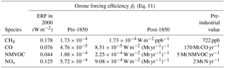
Tropospheric ozone is formed from a complex chemical reaction chain from emissions of CH₄, NO_x, CO and NMVOC. Furthermore, its concentration is more variable in space and time than for the well-mixed greenhouse gases. Therefore, we do not calculate a globally averaged concentration. We use coefficients from Stevenson et al. (2013) to estimate tropospheric ozone ERF from emissions of NO_x, CO and NMVOC, and concentrations of methane, assuming linearity between atmospheric burden and ozone forcing:

$$\begin{array}{ll}{\displaystyle }{F}_{{\mathrm{O}}_{\mathrm{3}}\text{tr}}& {\displaystyle }={\mathit{\beta }}_{{\mathrm{CH}}_{\mathrm{4}}}(C_{{\mathrm{CH}}_{\mathrm{4}}}-C_{{\mathrm{CH}}_{\mathrm{4}},\text{pi}})+{\mathit{\beta }}_{{\mathrm{NO}}_x}(E_{{\mathrm{NO}}_x}-E_{{\mathrm{NO}}_x,\text{pi}})\\ {\displaystyle }& {\displaystyle }+{\mathit{\beta }}_{\mathrm{CO}}(E_{\mathrm{CO}}-E_{\mathrm{CO},\text{pi}})+{\mathit{\beta }}_{\mathrm{NMVOC}}\\ \text{(11)}& {\displaystyle }& {\displaystyle }(E_{\mathrm{NMVOC}}-E_{\mathrm{NMVOC},\text{pi}})+f\left(T\right)\end{array}$$

and

$$\begin{array}{}\text{(12)}& f\left(T\right)=min\mathit{\{}\mathrm{0},\mathrm{0.032}\exp (-\mathrm{1.35}T)-\mathrm{0.032}\mathit{\}}.\end{array}$$

The β coefficients in Eq. (11) are provided in Table 4, and Eq. (12) is a small negative climate feedback, estimated using a curve fit to year 2000, 2030 and 2100 temperature changes under RCP8.5 in Stevenson et al. (2013). As Stevenson et al. (2013) used 1850 as their baseline for forcing calculations based on emissions data from Lamarque et al. (2010), in RCP scenarios adjusted coefficients can optionally be specified for times prior to 1850 where “pre-industrial” anthropogenic emissions are taken from Skeie et al. (2011). This ensures that ERF is both equal to zero in 1765 and equal to the best estimates in Stevenson et al. (2013) for 2005. Both the differing treatment prior to 1850 and the climate feedback can optionally be switched off by the user.

Table 4 Contribution to tropospheric ozone ERF from each precursor. Pre-industrial emissions from Skeie et al. (2011), pre-industrial CH₄ from Meinshausen et al. (2011b), 1850 and 2000 emissions from Lamarque et al. (2010), and 2000 minus 1850 ERF from Stevenson et al. (2013).

2.2.4 Stratospheric ozone

The stratospheric ozone ERF is calculated using the functional relationship borrowed from Meinshausen et al. (2011a), namely

$$\begin{array}{}\text{(13)}& F_{{\mathrm{O}}_{\mathrm{3}}\text{st}}=a(bs{)}^c.\end{array}$$

$a=-\mathrm{1.46}\times {\mathrm{10}}^{-\mathrm{5}}$, $b=\mathrm{2.05}\times {\mathrm{10}}^{-\mathrm{3}}$ and c=1.03 in Eq. (13) are fitting parameters that are found by a least-squares curve fit between Eq. (13) and the stratospheric ozone ERF time series from AR5; due to this data fitting approach, our parameters differ from MAGICC. s is the equivalent effective stratospheric chlorine (EESC) from all ozone-depleting substances, calculated as (Newman et al., 2007)

$$\begin{array}{}\text{(14)}& s=r_{\text{CFC}\mathrm{11}}\sum _{i\in \text{ODS}}\left(n_{\text{Cl}}\left(i\right)C_i{\displaystyle \frac{r_i}{r_{\text{CFC}\mathrm{11}}}}+\mathrm{45}{n}_{\text{Br}}\left(i\right)C_i{\displaystyle \frac{r_i}{r_{\text{CFC}\mathrm{11}}}}\right).\end{array}$$

r_i represents fractional release values for each ODS compound taken from Daniel and Velders (2011) and reproduced in Table 2. n_Cl and n_Br represent the number of chlorine and bromine atoms in compound i with the factor of 45 in Eq. (14) indicating that bromine is 45 times more effective at stratospheric ozone depletion than chlorine (Daniel et al., 1999). The concentrations C_i are expressed in ppb.

2.2.5 Stratospheric water vapour from methane oxidation

In AR5, the ERF from the stratospheric water vapour oxidation of methane was assumed to be 15 % of the methane ERF. This was based on the methane forcing relationship of Myhre et al. (1998), which is about 20 % lower than the Etminan et al. (2016) methane forcing used in FAIR. As there has been no substantial revision to the stratospheric water vapour forcing, we define stratospheric water vapour ERF as 12 % of the methane ERF.

2.2.6 Contrails

Meinshausen et al. (2011b) did not include a forcing time series for contrails or contrail-induced cirrus, which contribute a small positive ERF (Boucher et al., 2013). Three different methods to supply contrail ERF are available in FAIR: (1) scaling with aviation-based NO_x emissions, (2) scaling with global supply of jet kerosene fuel, or (3) supplying an external forcing time series. In method 1, it is assumed that contrail ERF is proportional to the aircraft NO_x emissions in a given year $E_{{\mathrm{NO}}_x,\text{avi}}$ compared to 2005 and multiplied by the 2005 ERF from Lee et al. (2009) of 0.0448 W m⁻²:

$$\begin{array}{}\text{(15)}& F_{\text{con}}={\displaystyle \frac{E_{{\mathrm{NO}}_x,\text{avi}}}{E_{{\mathrm{NO}}_x,\text{avi},\mathrm{2005}}}}{F}_{\text{con},\mathrm{2005}}.\end{array}$$

This gives a coefficient of $F_{\text{con},\mathrm{2005}}/E_{{\mathrm{NO}}_x,\text{avi},\mathrm{2005}}=\mathrm{0.0152}$ W m⁻² (Mt-aviNO_x yr⁻¹)⁻¹.

Method 2 is similar, based on kerosene fuel supplied S_kerosene, as a proxy for activity data. We take a 2005 global kerosene supply of 236 Gt from International Energy Agency (2018) to anchor the forcing time series calculation:

$$\begin{array}{}\text{(16)}& F_{\text{con}}={\displaystyle \frac{S_{\text{kerosene}}}{S_{\text{kerosene},\mathrm{2005}}}}{F}_{\text{con},\mathrm{2005}}.\end{array}$$

For method 1, the past and future aviation NO_x emissions from the RCP scenarios are available in FAIR. The fraction of total NO_x emissions attributable to aviation is used to calculate $E_{{\mathrm{NO}}_x,\text{avi}}$ in Eq. (15).

2.2.7 Aerosols

Aerosols have a lifetime of the order of days (Kristiansen et al., 2016), and the emissions are converted to forcing without an intermediate concentration step.

The aerosol ERF contains contributions from aerosol-radiation interactions (ERFari) and from aerosol–cloud interactions (ERFaci). ERFari includes the direct radiative effect of aerosols, in addition to rapid adjustments due to changes in the atmospheric temperature, humidity and cloud profile (formerly the semi-direct effect; Boucher et al., 2013).

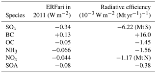
We use the multi-model results from Aerocom (Myhre et al., 2013a) and assume a linear relationship between emissions and forcing:

$$\begin{array}{ll}{\displaystyle }{F}_{\text{ari}}& {\displaystyle }={\mathit{\gamma }}_{\text{BC}}{E}_{\text{BC}}+{\mathit{\gamma }}_{\text{OC}}{E}_{\text{OC}}+{\mathit{\gamma }}_{{\text{SO}}_x}{E}_{{\text{SO}}_x}+{\mathit{\gamma }}_{{\text{NO}}_x}{E}_{{\text{NO}}_x}\\ \text{(17)}& {\displaystyle }& {\displaystyle }+{\mathit{\gamma }}_{{\text{NH}}_{\mathrm{3}}}{E}_{{\text{NH}}_{\mathrm{3}}}+{\mathit{\gamma }}_{\text{SOA}}{E}_{\text{NMVOC}},\end{array}$$

where the default coefficients for each γ are provided in Table 5 and calculated from the difference in anthropogenic emissions between 1765 and 2010. Users are free to specify their own species-dependent γ for each aerosol precursor. We assume that emitted black carbon (BC) and organic carbon (OC) correspond directly to BC and OC forcing and that emissions of sulfur compounds (SO_x) correspond directly to sulfate forcing. Following Shindell et al. (2009) we assume a 60 % contribution to nitrate aerosol forcing from NH₃ and 40 % from NO_x. We allow formation of secondary organic aerosol (SOA) to scale with emissions of anthropogenic NMVOC. Biomass burning aerosol has a net zero forcing in 2011 and is ignored, and mineral dust, which does not scale directly with an emitted component, is also disregarded. The sum of the direct effects of each component is −0.35 W m⁻² in 2010 assuming RCP4.5. The difference between this and the best-estimate ERFari of −0.45 W m⁻² in AR5 is assumed to be due to rapid adjustments (semi-direct effects). There is evidence that scattering aerosols do not exhibit significant semi-direct effects (Boucher et al., 2013), so the overall difference of −0.1 W m⁻² is assumed to be due to BC semi-direct effects. The net impact is to reduce the radiative efficiency coefficient of BC.

Table 5 Contribution to ERFari from each aerosol precursor species and contribution to 2011 ERFari.

ERFaci describes how aerosols affect clouds in the radiation budget; the two main mechanisms are changes in cloud droplet size, which changes cloud albedo (Twomey, 1977) and changes in cloud lifetime and precipitation efficiency, which affects cloud fraction (Albrecht, 1989; Boucher et al., 2013). There is evidence that the ERFaci is not linear with emissions (Carslaw et al., 2013), and as such a simple linear scaling as for ERFari may not be appropriate.

In FAIR we use an emulation of the global aerosol model of Ghan et al. (2013) to estimate ERFaci from precursor emissions. The Ghan et al. (2013) method contains a series of non-linear equations that require iterative solutions and currently has not been optimised for use in FAIR. We therefore emulate the ERFaci by varying the emissions of SO_x and primary organic aerosol (the sum of BC and OC). Secondary organic aerosol is also an input to the model, but it is found that ERFaci is only weakly dependent on NMVOC emissions and a simple functional form could not be found and so was eliminated as a predictor.

Informed by the simple aerosol model of Stevens (2015), we use a logarithmic dependence of ERFaci on emissions that can vary both as a function of SO_x and BC+OC, which represents increasing saturation of the cloud–albedo effect with increasing emissions. We find a relationship of the form

$$\begin{array}{ll}{\displaystyle }G(E_{{\mathrm{SO}}_x},& {\displaystyle }{E}_{\mathrm{BC}+\mathrm{OC}})=-\mathrm{1.95}\log \\ \text{(18)}& {\displaystyle }& {\displaystyle }(\mathrm{1}+\mathrm{0.0111}{E}_{{\mathrm{SO}}_x}+\mathrm{0.0139}{E}_{\mathrm{BC}+\mathrm{OC}}),\end{array}$$

where the coefficients in Eq. (18) are found with a least-squares optimisation routine (r²=0.938). The modelled and simulated outputs are compared in Fig. S1 in the Supplement.

Equation (18) was derived from a climate model and produces a present-day ERFaci that is stronger than the central estimate of −0.45 W m⁻² from AR5. We therefore scale Eq. (18) in order to obtain a forcing of −0.45 W m⁻² in 2011 under RCP4.5 emissions:

$$\begin{array}{}\text{(19)}& F_{\text{aci}}=-\mathrm{0.45}{\displaystyle \frac{G\left(E\right)-G\left(E_{\mathrm{1765}}\right)}{G\left(E_{\mathrm{2011}}\right)-G\left(E_{\mathrm{1765}}\right)}},\end{array}$$

where $E=(E_{{\mathrm{SO}}_x},E_{\mathrm{BC}+\mathrm{OC}})$ refers to emissions and a numerical subscript refers to a particular year. The emissions for 1750 from Skeie et al. (2011) are used for year 1765, and a linear interpolation between 1765 and 1850 is applied.

2.2.8 Black carbon on snow

The best-estimate ERF of 0.04 W m⁻² in AR5 for 2011 is compared to the BC emissions in 2011 from Meinshausen et al. (2011b), with this scaling factor assumed to hold for all years. The relationship is given by

$$\begin{array}{}\text{(20)}& F_{\text{BCsnow}}=\mathrm{0.00494}{E}_{\text{BC}},\end{array}$$

where E_BC is BC emissions in Mt yr⁻¹.

2.2.9 Land use change

Land use forcing is a result of surface albedo change (Andrews et al., 2017) and changes in evapotranspiration patterns (Jones et al., 2015), which is often due to deforestation for agriculture (Myhre and Myhre, 2003). Cropland has a higher albedo than the forest that it replaces, reflecting more incident solar radiation and therefore resulting in a negative ERF; additionally, deforestation in boreal regions may unmask snow-covered ground, again increasing albedo.

Deforestation produces land-use-related CO₂ emissions. The total amount of deforestation since pre-industrial times could therefore be expected to scale with cumulative land-use-related CO₂ emissions. This is the default approach taken in FAIR. A regression of non-fossil CO₂ emissions against land use ERF in AR5 gives

$$\begin{array}{}\text{(21)}& F_{\text{landuse}}=-\mathrm{1.14}\times {\mathrm{10}}^{-\mathrm{3}}\sum _{j=\mathrm{0}}^t{E}_{{\text{CO}}_{\mathrm{2}}\text{land},j},\end{array}$$

where the coefficient has units W m⁻² (Gt C)⁻¹.

The simple relationship in Eq. (21) does not take into account latitude dependence of surface albedo or any evapotranspiration changes. As a zero-dimensional model, FAIR does not include geographical dependence of individual forcing effects, which may differ significantly between forcing pathways (for example the scenarios typically used to drive integrated assessment models). Inclusion of evapotranspiration effects, which again differ between tropical and boreal regions (Jones et al., 2015), is challenging as they do not directly relate to an emitted species or a change in radiative forcing (Pielke et al., 2002). Nevertheless, we conclude that this simple treatment is acceptable, firstly as the range of land use forcing uncertainty is relatively large (so much that the sign of the forcing is not known with confidence; Myhre et al., 2013b), secondly because at least in the best estimate the forcing is a small fraction of the present-day total, and thirdly because the future trajectory of the land use forcing in the RCP datasets is very similar to that predicted by FAIR, suggesting that a dependence on cumulative land use CO₂ emissions is an important component of the land use forcing in MAGICC.

Noting that this simple relationship may not be suitable in all cases, the user is free to supply their own time series of ERF from land use change. If gridded land use data are available, the transitions to and from forested land each year can be convoluted with the marginal contribution to land use forcing per square kilometre deforestation (e.g. from Jones et al., 2015).

2.2.10 Solar variability

The SOLARIS-HEPPA v3.2 solar irradiance dataset prepared for CMIP6 is used to generate the solar ERF, which includes projections of the variation in future solar cycles from 1850 to 2300 (Matthes et al., 2017). ERF from solar forcing is calculated as the change in solar constant since 1850 divided by 4 (average insolation) and multiplied by 0.7 (representing planetary co-albedo). This approach is also used in Meinshausen et al. (2011b). Prior to 1850, we revert to the solar forcing from AR5.

2.2.11 Volcanic aerosol

Historical volcanic forcing is punctuated by several large eruptions that cause large but short-lived negative forcing episodes, with several smaller eruptions that cause year-to-year changes in the volcanic forcing. In order to generate a historical volcanic ERF time series, we first start with gridded volcanic optical depths taken from the Easy Volcanic Aerosol generator over the 1850–2014 period (Toohey et al., 2016) which will be used to drive CMIP6 models. A number of time slice experiments with various scalings of the historical mean volcanic optical depth are run in the HadGEM3-GA7.1 climate model (Walters et al., 2017), where it was found that aerosol ERF scales as −18τ_vol (where τ_vol is globally averaged volcanic aerosol optical depth at 550 nm). This scaling factor is consistent with other HadGEM models (Gregory et al., 2016), although weaker than the value of −26τ_vol adopted in AR5. The discrepancy is claimed to be due to rapid adjustments, in which case our adoption of the less negative value is consistent with the ERF definition.

In the context of measuring forcing since the pre-industrial, we have to assume an “average” level of volcanic background aerosol. We therefore define the 1850–2014 period to have a mean volcanic forcing of zero. To achieve this we subtract the mean (negative) forcing from the historical period, resulting in a quiescent year ERF of around +0.1 W m⁻². A similar approach was taken in Meinshausen et al. (2011b), with a higher quiescent year forcing of about +0.2 W m⁻². Prior to 1850 we use the AR5 dataset, scaled by 18/26 to match the differences in optical depth/forcing relationships, and from 2015 onwards volcanic forcing is defined to be zero. For solar and volcanic forcing, users are free to provide a custom forcing time series or to use the AR5 or RCP datasets which are both available in FAIR.

2.3 Temperature change

In simple impulse response models, forcing is related to total temperature change in year t, T_t, by a two-time constant model (Boucher and Reddy, 2008; Myhre et al., 2013b; Millar et al., 2015, 2017). FAIR v1.3 takes this approach with a small modification compared to FAIR v1.0 to allow for forcing-specific efficacies ϵ_j such that

$$\begin{array}{ll}{\displaystyle }{T}_{t,i}=& {\displaystyle }{T}_{t-\mathrm{1},i}\exp \left(\mathrm{1}/d_i\right)+\sum _{j=\mathrm{0}}^{\mathrm{12}}\left(q_i{\mathit{ϵ}}_j{F}_j\left(\mathrm{1}-\exp (\mathrm{1}/d_i)\right)\right);\\ \text{(22)}& {\displaystyle }& {\displaystyle }i=\mathrm{1},\mathrm{2}.\end{array}$$

Owing to the use of ERF rather than RF in FAIR v1.3 and its better correspondence with temperature, efficacies are assumed to be unity for all forcing agents except black carbon on snow (j=9), where an efficacy of 3 is used following Bond et al. (2013). The coefficients d₁ and d₂ govern the slow (i=1) and fast (i=2) temperature changes from a response to forcing from the upper ocean and the deep ocean respectively (Millar et al., 2015). The total temperature change in year t is the sum of the slow and fast components, i.e. $T_t=T_{t,\mathrm{1}}+T_{t,\mathrm{2}}$. F_j represents the 13 individual forcing agents in year t calculated in Sect. 2.2 (see also Table 3). d₁ and d₂ default to 239 and 4.1 years which are fit to match the mean of CMIP5 models (Geoffroy et al., 2013). The coefficients q₁ and q₂ (units K W⁻¹ m²) are determined by solving a matrix equation given transient climate response (TCR), equilibrium climate sensitivity (ECS), d₁, d₂ and the ERF from a doubling of CO₂, $F_{\mathrm{2}\times }=\mathrm{3.71}$ W m⁻² (Myhre et al., 2013b):

$$\begin{array}{ll}\text{(23)}& {\displaystyle }{T}_{\text{ECS}}=& {\displaystyle }{F}_{\mathrm{2}\times }(q_{\mathrm{1}}+q_{\mathrm{2}});{\displaystyle }{T}_{\text{TCR}}=& {\displaystyle }{F}_{\mathrm{2}\times }\left(q_{\mathrm{1}}\left(\mathrm{1}-{\displaystyle \frac{d_{\mathrm{1}}}{D}}\left(\mathrm{1}-\exp \left(-{\displaystyle \frac{D}{d_{\mathrm{1}}}}\right)\right)\right)\right.\\ \text{(24)}& {\displaystyle }& {\displaystyle }\left.+q_{\mathrm{2}}\left(\mathrm{1}-{\displaystyle \frac{d_{\mathrm{2}}}{D}}\left(\mathrm{1}-\exp \left({\displaystyle \frac{D}{d_{\mathrm{2}}}}\right)\right)\right)\right),\end{array}$$

giving the relative contributions to the fast and slow components of the warming. $D=\log \left(\mathrm{2}\right)/\log \left(\mathrm{1.01}\right)\approx \mathrm{69.7}$ years is the time to a doubling of CO₂ with a compound 1 % per year increase in CO₂ concentrations.

There is some evidence that ECS and TCR have not been constant values over the historical period (Gregory and Andrews, 2016; Gregory et al., 2015) and that ECS does not necessarily assume a constant value in CMIP5 modelling experiments (Armour, 2017). FAIR has the capability to model time-evolving ECS and TCR by updating the q₁ and q₂ values in each time step.

3 Projections using a large ensemble

To test the model response to a range of forcing pathways, we perform a 100 000-member Monte Carlo simulation using emissions from the RCP datasets (Meinshausen et al., 2011b). Emissions themselves are not altered from the RCP time series, but the TCR, ECS, carbon cycle response to increasing temperature (r_T) and cumulative emissions (r_C) along with the pre-industrial value of iIRF₁₀₀ (r₀), plus the ERF scale factors for each of the 13 forcing agents, are drawn from distributions. FAIR is run from 1765 (the start of the RCP emissions datasets) to 2100.

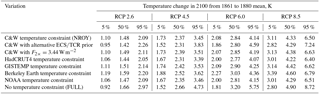
3.1 Constraint to historical temperature observations

As a wide range of forcing, and thus temperature, scenarios can be generated, there are a proportion of ensemble members generated that fall outside the range of plausibility. We constrain the full 100 000-member ensemble (hereafter FULL) to the observed temperature change from the Cowtan and Way (2014) dataset (hereafter C&W) to assess plausibility; ensemble members that satisfy the temperature constraint are designated as “not ruled out yet” (NROY) and the majority of the discussion of the results in Sect. 4 focuses on this dataset. We rebase all of the temperatures to the 1861–1880 mean following Richardson et al. (2016), to represent a pre-industrial state that is relatively free of volcanic eruptions but with a reasonable global coverage of temperature observations. An ordinary least-squares regression of temperature change versus time from 1880 to 2016 is used to calculate the linear warming trend in each ensemble member. The regression is also performed for the C&W “observational” dataset to estimate the observed warming rate. The confidence interval around the C&W warming rate is inflated by a factor that represents the lag-1 autocorrelation of residuals (i.e. the trend-line estimate from the regression minus the C&W “observations”) which accounts for internal climate variability (Santer et al., 2008; Thompson et al., 2015) and is the same method used in AR5 to estimate linear temperature trends. The constraint is satisfied for an ensemble member if the modelled trend falls within the 5–95 % range of trend from C&W of 0.95±0.17 K.

The C&W observed warming from 1880 to 2016 is higher than the UK Met Office Hadley Centre observational dataset (HadCRUT4; Morice et al. 2012) estimate of 0.91±0.18 K for the same time frame. The infilling of grid boxes where no or limited data are available accounts for these differences, as sparse observations are typically in polar regions which warm faster than the global mean (Cowtan and Way, 2014). Under this constraint approximately 26 % of the FULL ensemble is retained in NROY.

It should be stressed that there are several issues to consider when attempting to derive plausible parameter sets from observational data. These include the type of observational constraints to employ (Meinshausen et al., 2009), the length of the historical record (e.g. Otto et al., 2013), the separation of forced response from natural variability (Haustein et al., 2017) and assumptions surrounding prior distributions (Frame et al., 2005).

3.2 Sampling ECS and TCR

The ECS and TCR from CMIP5 models (Forster et al., 2013) are used to generate a joint log-normal distribution. Random variables are sampled using the R package MethylCapSig¹ using the mean, standard deviation and correlation coefficient (r=0.81) between ECS and TCR in CMIP5. A log-normal distribution is representative of distributions of ECS and TCR in the literature (Meinshausen et al., 2009; Rogelj et al., 2012; Flato et al., 2013; Millar et al., 2017). The sampled joint and marginal distributions are shown as black contours and curves in Fig. 3. We sample 100 000 ECS–TCR pairs; sampled pairs where ECS < TCR are rejected and redrawn. A joint distribution is used because ECS and TCR are highly correlated and low values of the realised warming fraction (TCR divided by ECS) are inconsistent with models and observations (Millar et al., 2015). For other sampled quantities in this section a 100 000-member ensemble is also generated.

3.3 Sampling thermal response and carbon cycle parameters

We allow F_2×, the ERF due to a doubling of CO₂, to assume a Gaussian distribution with 5–95 % confidence interval of 20 % around the best-estimate ERF of 3.71 W m⁻² (Myhre et al., 2013b). d₁ (mean 239 years, standard deviation 63 years) and d₂ (mean 4.1 years, standard deviation 1.0 years) in Eq. (22) are also varied based on truncated Gaussian distributions (no values outside ±3σ allowed, primarily to prevent unrealistically small or negative values of the slow response d₁). Although FAIR is able to model the response to time-varying ECS and TCR, we use time-invariant values in our ensemble.

Some uncertainty in the carbon cycle parameters is assumed with samples of r₀, r_C and r_T taken from Gaussian distributions. r₀, r_C and r_T are given 5–95 % confidence intervals of 13 % of the default parameter value following Millar et al. (2017).

3.4 Sampling ERF uncertainties

The uncertainty in each of the 13 forcing components is modelled following the 5–95 % confidence intervals for each forcing from AR5 (Myhre et al., 2013b, Table 8.6) in 2011 (Table 3). This is achieved by scaling the ERF values calculated in Sect. 2.2; the uncertainty ranges are given in Table 3. The scaling factor is applied to the whole time series. A time-varying scale factor for forcing can be used, and an option is provided to exactly replicate the AR5 historical time series for each component, but we do not apply it here. Most uncertainties are assumed to be Gaussian, the exceptions being contrails and BC on snow which are log-normally distributed (with geometric standard deviations 1.92 and 1.65 respectively, following AR5) and aerosols which are modelled as two half-Gaussian distributions, treating values above and below the best estimate separately. These ERF uncertainties are assumed to be uncorrelated with each other.

4 Results from the NROY ensemble for the RCP scenarios

4.1 ECS and TCR

The FULL and NROY joint and marginal distributions of ECS and TCR are shown in Fig. 3.

The temperature constraint in NROY results in distributions of ECS and TCR that are lower than in FULL. Some of the prior sample space in which ECS and TCR are larger than the likely AR5 ranges has been rejected in the NROY distribution. While the possibility that ECS > 5 K cannot be ruled out, it appears less likely than would be inferred from CMIP5 models, although it should be stressed that time-varying feedbacks are not accounted for in this large ensemble, which would allow ECS to increase over time (Armour, 2017). From the marginal distributions, we estimate that ECS and TCR are 2.86 (2.01 to 4.22) K and 1.53 (1.05 to 2.41) K (median; (5–95 % range)) respectively in the NROY ensemble, similar to but a little more tightly constrained than the likely AR5 (>66 % probability) ranges of 1.5 to 4.5 K and 1.0 to 2.5 K, noting that the AR5 ranges are estimated from a combination of models, observations and expert judgement. The ratio of TCR to ECS, the realised warming fraction (RWF), is approximately independent of TCR in CMIP5 models (Millar et al., 2015), and the prior distribution could alternatively be defined in terms of the TCR and RWF joint distribution, which is explored in Sect. 5. The FULL and NROY median and 5 to 95 % ranges of RWF are 0.56 (0.41 to 0.76) and 0.54 (0.40 to 0.72) respectively, which is close to the range of CMIP5 models (0.45 to 0.75, Millar et al., 2017).

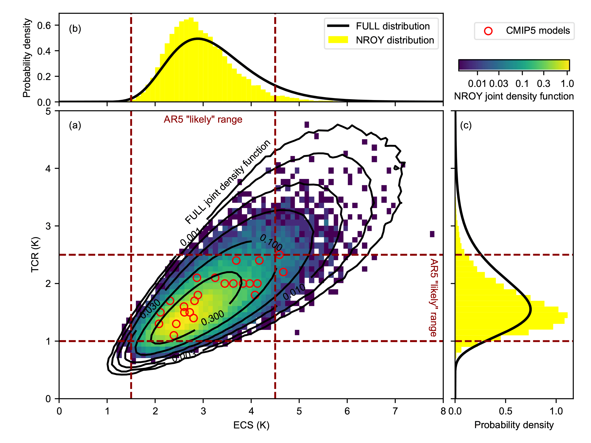
Figure 3 (a) Joint distributions (FULL and NROY) of ECS and TCR. (b) Marginal distributions of ECS. (c) Marginal distributions of TCR. In (a), the FULL distribution is shown with open black contours and the NROY distribution with coloured squares. Probability density is plotted on a log scale. In (b) and (c), the FULL distribution is shown as a black curve and the NROY distribution with yellow histogram bars, both plotted on a linear scale. The NROY distributions contains only those ensemble members which agree with the C&W observed historical temperatures. CMIP5 models are depicted with red circles.

4.2 Historical and future greenhouse gas concentrations

The historical (1765–2005) greenhouse gas concentrations from the RCP scenarios in Meinshausen et al. (2011b) were assimilated from observations of in situ and ice core records and represent a best estimate of the actual concentrations over this period. We therefore assume that the RCP data represents the best estimate of the historical concentrations and compare our estimates from the NROY ensemble using the emissions-driven model.

The FAIR model reproduces the historical concentrations of greenhouse gases (Fig. 4). The atmospheric concentrations of CO₂ estimated from FAIR are up to 9 ppm lower than MAGICC6 in the period 1880–1950 (Fig. 4a). A simple carbon cycle model cannot reproduce the kinks in the observational CO₂ trend without large changes in the input emissions. However, between 1950 and 2005, the differences between the two curves are small. The post-2005 atmospheric CO₂ concentrations are slightly higher than those estimated by MAGICC6 for the RCP scenarios, but the MAGICC6 concentrations are within the uncertainty range from the NROY ensemble. FAIR projects best-estimate CO₂ concentrations of 427 (413 to 443), 552 (527 to 578), 695 (661 to 731) and 979 (926 to 1040) ppm for RCP2.6, RCP4.5, RCP6 and RCP8.5 in 2100. Here, the uncertainty in CO₂ concentrations relates to the range of carbon cycle parameters and the temperature dependence on carbon uptake sampled in the large ensemble.

The historical CH₄ and N₂O concentrations in FAIR have been tuned to agree with Meinshausen et al. (2011b) by adjusting natural emissions as described previously (Fig. 4b, c). There are some small differences in the future CH₄ and N₂O concentrations in the RCPs using fixed atmospheric lifetimes and constant (present-day) natural emissions.

Kyoto Protocol gases have been grouped as HFC134a-eq based on their radiative efficiency, and ODSs have been similarly grouped as CFC12-eq (Fig. 4d, e). Small differences between the models in future scenarios may be a result of the assumption of a change in the rate of the Brewer–Dobson circulation in MAGICC6 (Meinshausen et al., 2011a), which increases the efficiency of the stratospheric sink for these gases. This temperature-dependent effect is not included in FAIR. Over the historical period, the differences are a result of the natural emissions of CF₄ (contributing to HFC134a-eq) and CH₃Br and CH₃Cl (contributing to CFC12-eq) providing a non-zero background state of these greenhouse gas equivalents in FAIR. In the RCP historical dataset these background concentrations have not been added to the HFC134a-eq and CFC12-eq time series.

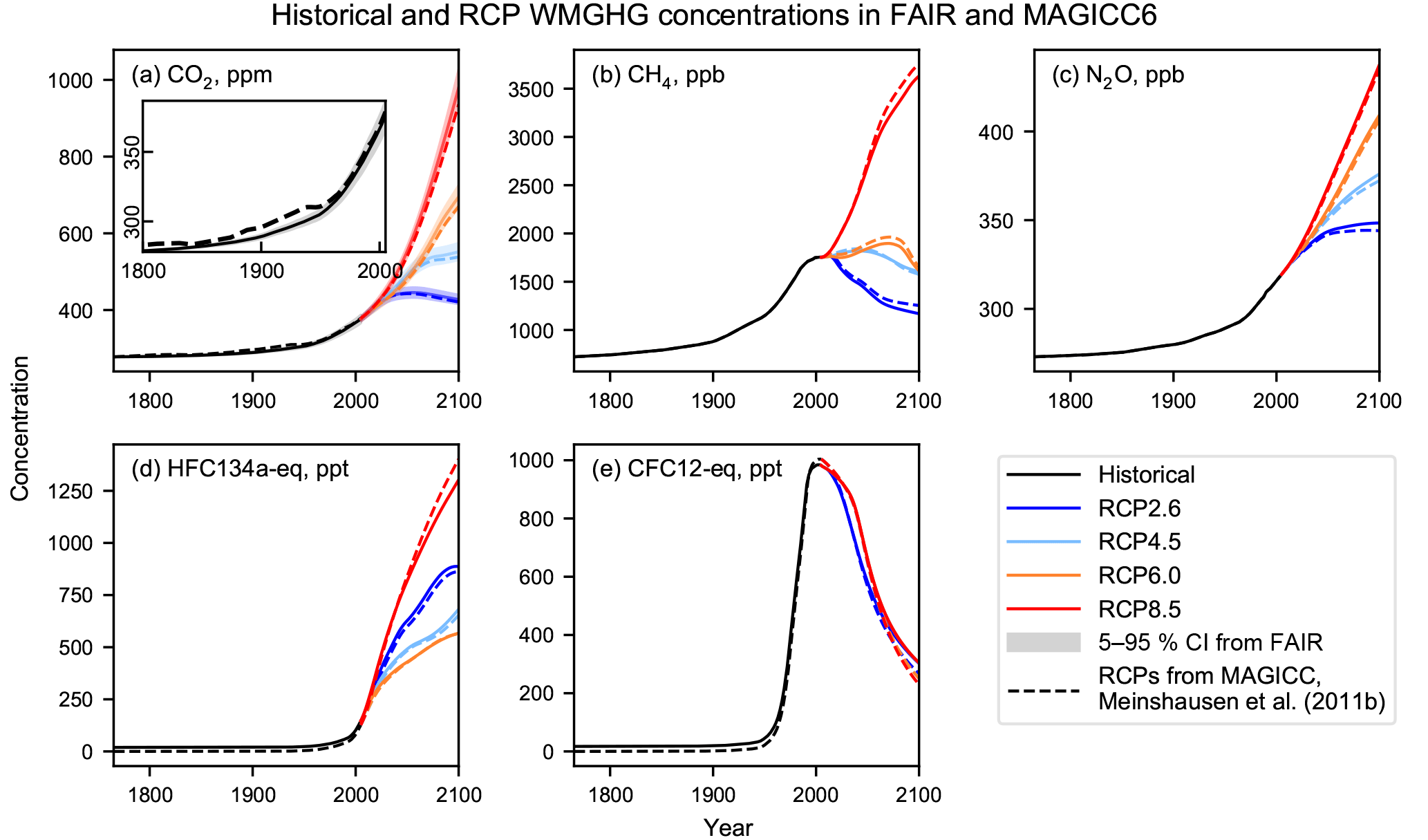
Figure 4 Comparison of the historical and RCP greenhouse gas concentrations in FAIR (heavy solid lines) with 5–95 % confidence intervals (shading) for CO₂. Dashed lines show the concentrations from MAGICC6 (Meinshausen et al., 2011b). For CFC12-eq, the RCP4.5 and RCP6.0 lines lie underneath the RCP8.5 line.

4.3 Historical, present and future radiative forcing

Figure 5 shows the comparison between FAIR and MAGICC6 for the 13 forcing agents considered in FAIR for the NROY ensemble. The ERF time series for the historical period in AR5 is also shown (IPCC, 2013). The updated radiative forcing relationship for CH₄ increases radiative forcing substantially (Fig. 5b). The new relationship for N₂O results in a slightly lower ERF estimate in FAIR than RF in MAGICC6 (Fig. 5c), which is offset by the higher concentrations of N₂O in FAIR. The FAIR estimate of CO₂ forcing is also higher than MAGICC for the RCPs, but the ERFs from FAIR and RFs from MAGICC for the minor greenhouse gases are similar (Fig. 5a, d). For non-CO₂ gases, AR5 did not provide a breakdown of ERF by individual gas, so the total ERF has been scaled by the ratios in the MAGICC6 time series.

For tropospheric ozone, the Stevenson et al. (2013) relationship agrees well with AR5 until around 1970, from which point it is larger than AR5. There is also a large relative difference between this relationship and the MAGICC estimate in AR5 out to 2100 (Fig. 5e). The shape of the stratospheric ozone ERF curve between AR5 and MAGICC6 differs, but it can be seen that the AR5 historical ERF is well emulated as it uses the same functional relationship as AR5 (Fig. 5f). Stratospheric water vapour from methane oxidation depends on the underlying methane forcing and is similar to the AR5 time series (Fig. 5g). Contrail ERF shows a similar time evolution over the historical period to AR5 (Fig. 5h). Historically, ERF from aviation contrails has been small but may become more substantial in the future. The median aerosol ERF in FAIR is slightly more negative than in AR5 from around 1900 to 2011 (Fig. 5i) but is less negative than the RCP projections. We reiterate here that the RCPs report RF from MAGICC rather than ERF.

BC on snow has a smaller ERF in FAIR than the corresponding RF in MAGICC6, although the efficacy factor of 3 used in FAIR results in a similar effect on temperature between the models (Fig. 5j). Estimates of future land use forcing in FAIR follow a similar shape to the Meinshausen et al. (2011b) dataset, with slightly less negative best estimates to the AR5 ERF 2011 best estimate; agreement in the historical period to either MAGICC6 or AR5 is less good, but the general trajectory of forcing is correct (Fig. 5k). There are substantial differences between the volcanic forcing datasets in FAIR, AR5 and the RCPs that are not easy to discern at the resolution of the plot (Fig. 5l): generally, the AR5 dataset gives more negative forcing than the RCPs during volcanically active years and also defines the absence of volcanoes as zero forcing whereas the RCP and FAIR datasets define zero to be the average of the historical period. Solar forcing is used from the new CMIP6 dataset, which is reasonably similar to the RCP time series for historical forcing but exhibits some differences in the future owing to the assumed inter-cycle variability that was not present in CMIP5 (Fig. 5m).

Figure 5n shows the sum of the forcing components. The best-estimate sum of ERF follows AR5 closely over the historical period, which is intentional. In the RCP future scenarios, the FAIR best estimates of ERF are higher than the corresponding RF estimates in MAGICC. This is in part due to the increased CH₄, tropospheric ozone and contrail forcing in FAIR, and less negative total aerosol ERF. The FAIR model projects 2100 ERFs (median (5–95 % credible intervals)) of 2.62 (1.79 to 3.64), 4.62 (3.30 to 6.22), 5.84 (4.07 to 8.00) and 9.34 (6.84 to 12.44) W m⁻² for RCP2.6, RCP4.5, RCP6.0 and RCP8.5 respectively.

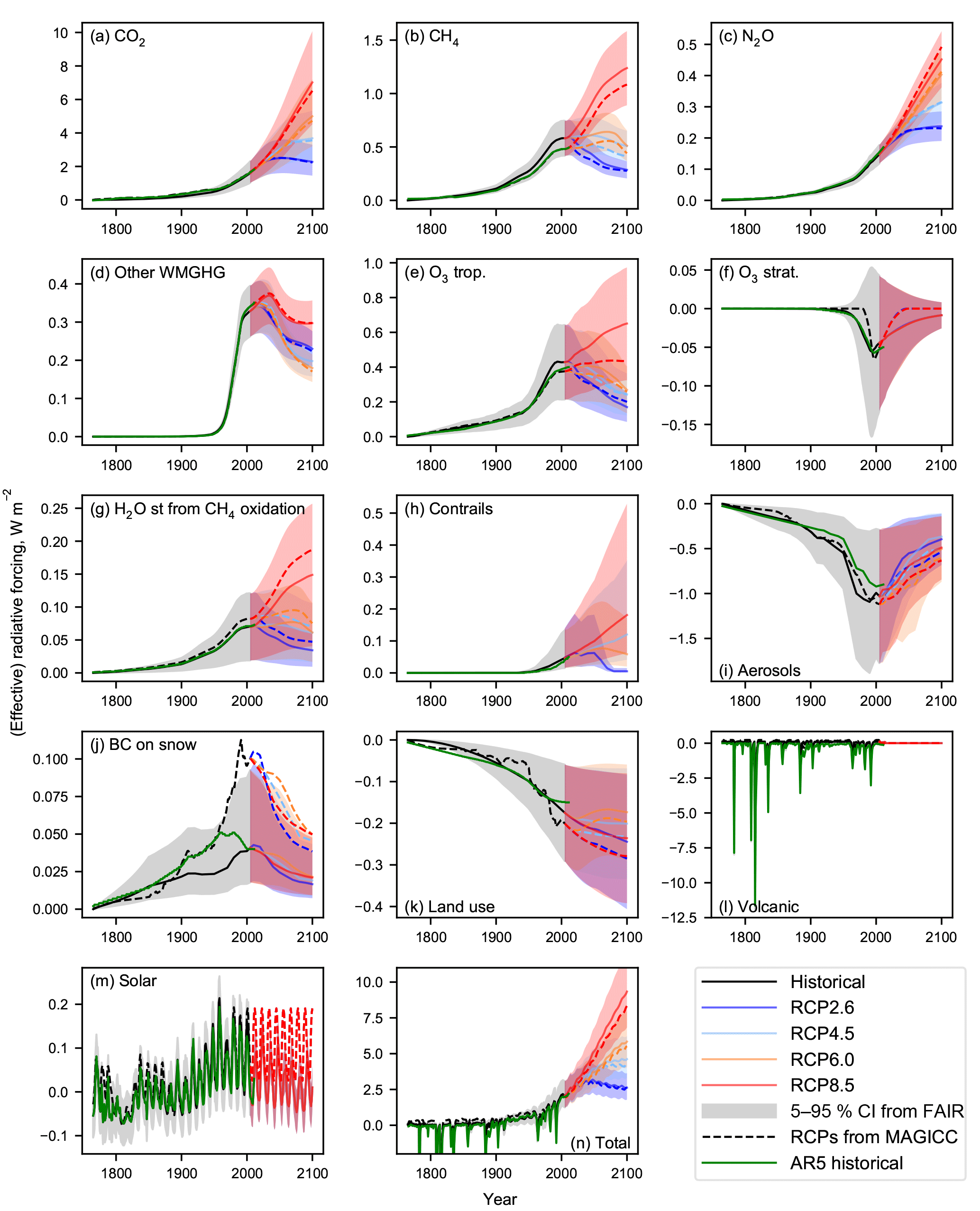
Figure 5 Comparison of the radiative forcing from RCP2.6, RCP4.5, RCP6.0 and RCP8.5 derived from 13 separate components (a–m), along with the total radiative forcing (n). ERF from FAIR (solid lines) with 5–95 % confidence intervals (shading), RF from MAGICC6 (dashed lines; Meinshausen et al., 2011b) and RF from AR5 Annex II for 1850–2011 (green solid lines, IPCC, 2013).

4.4 Relationship between forcing components, ECS and TCR

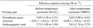
The distribution of ERF in 2017 for aerosols, greenhouse gases and the anthropogenic total in both the FULL and the NROY ensembles assuming the RCP8.5 forcing pathway is shown in Fig. 6 and Table 6. The temperature constraint in NROY permits a wider range of greenhouse gas ERF than the FULL ensemble. For aerosols, the distribution of ERF in NROY is again slightly wider than in FULL. The median estimate of net anthropogenic ERF of 2.63 W m⁻² in 2017 for NROY is a little lower than the unconstrained FULL estimate of 2.73 W m⁻² with a wider uncertainty range.

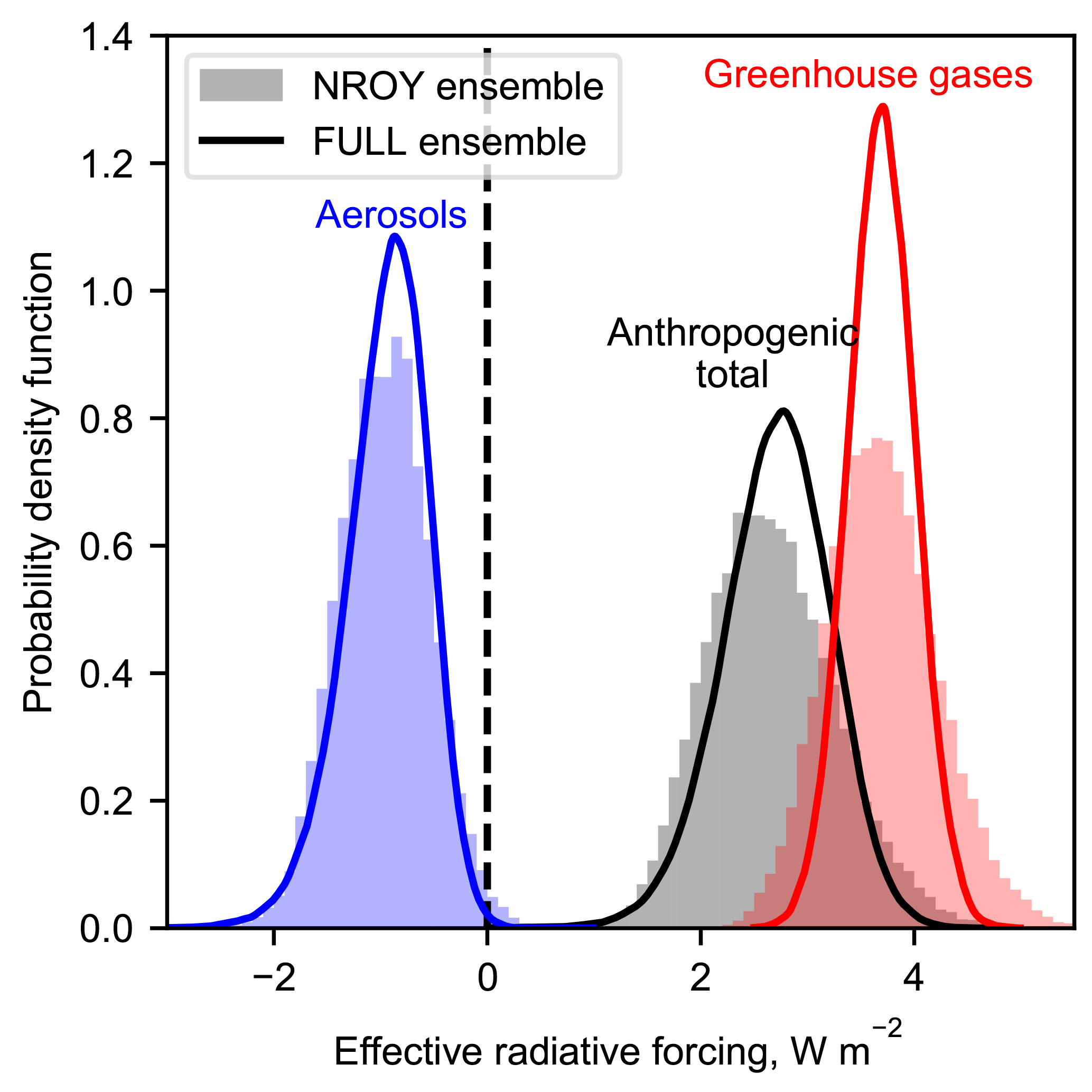
Figure 6 ERF from aerosols (blue), greenhouse gases (red) and total anthropogenic (black) for present-day (2017, based on RCP8.5) runs from FAIR constrained to observed temperature change (NROY; histograms) and from prior distributions (FULL; curves); compare Myhre et al. (2013b, Fig. 8.16). Greenhouse gas forcing includes contributions from ozone and stratospheric water vapour from methane. Anthropogenic total is the sum of greenhouse gas, aerosol, contrails, BC on snow and land use change. The latter three distributions are not shown separately.

Table 6 Median and 5–95 % credible intervals for effective radiative forcing from greenhouse gases, aerosols and anthropogenic total from the FULL and NROY FAIR ensembles in 2017. Anthropogenic total contains contributions from contrails, BC on snow and land use change and therefore is not equal to the sum of greenhouse gas and aerosol forcing. Compare Fig. 6.

There are negative correlations between aerosol radiative forcing and ECS∕TCR (Fig. 7). A large negative aerosol forcing requires a high ECS to balance and recreate realistic observed temperatures (Forest et al., 2006). Millar et al. (2015) highlighted the necessity of anti-correlation between TCR and aerosol forcing in observational constraints. The aerosol forcing on TCR constraint is tighter than that on ECS, evidenced by the narrower mass of points in the TCR plot (Fig. 7b) compared to the ECS plot (Fig. 7a). A high value for TCR (greater than 2.5 K) or ECS (greater than 5 K) is only possible with a strong negative present-day aerosol forcing (more negative than about −1.0 W m⁻²).

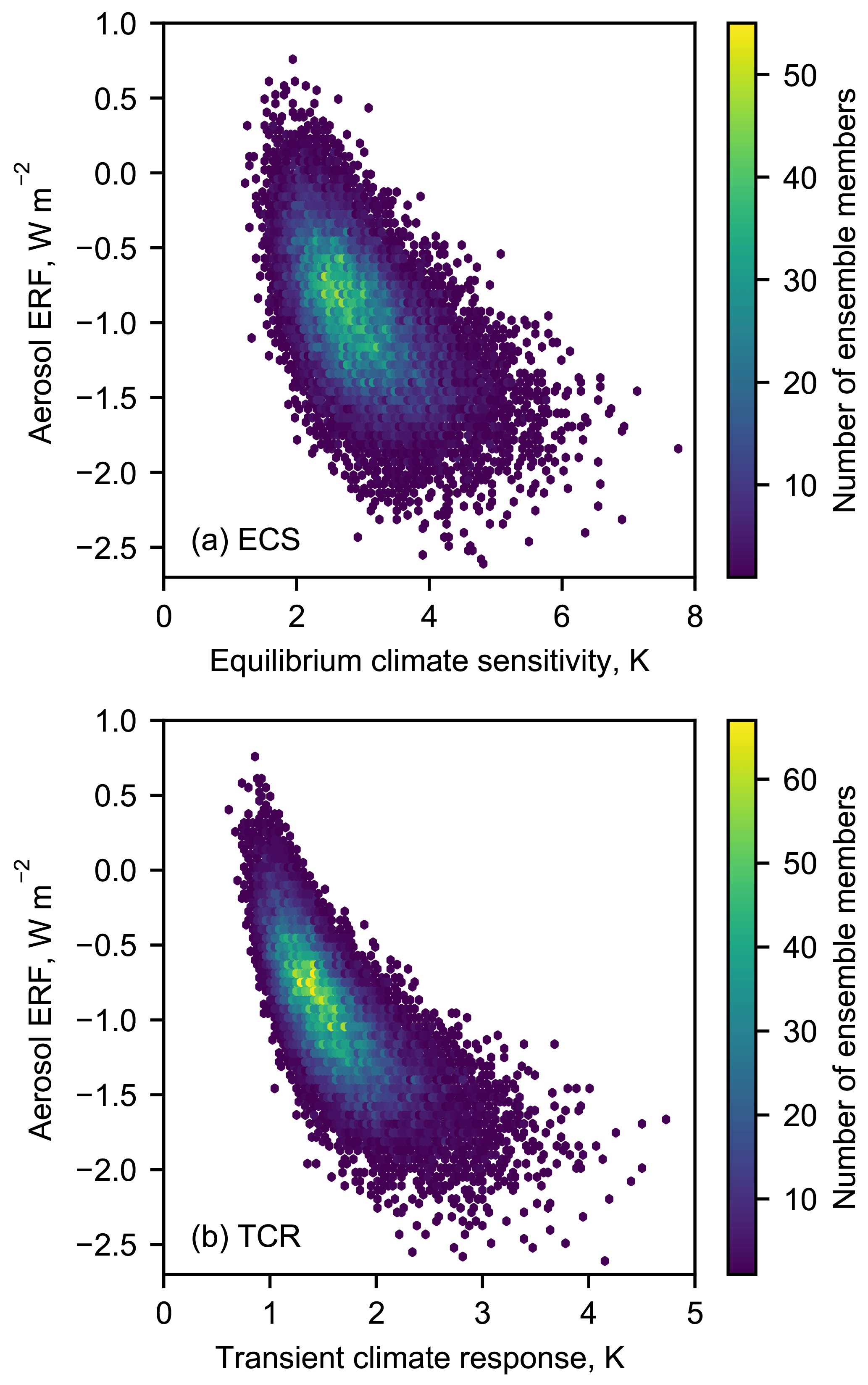
Figure 7 Relationship between (a) ECS and aerosol ERF; (b) TCR and aerosol ERF for the NROY ensemble. Aerosol ERF is shown for 2017 under the RCP8.5 scenario.

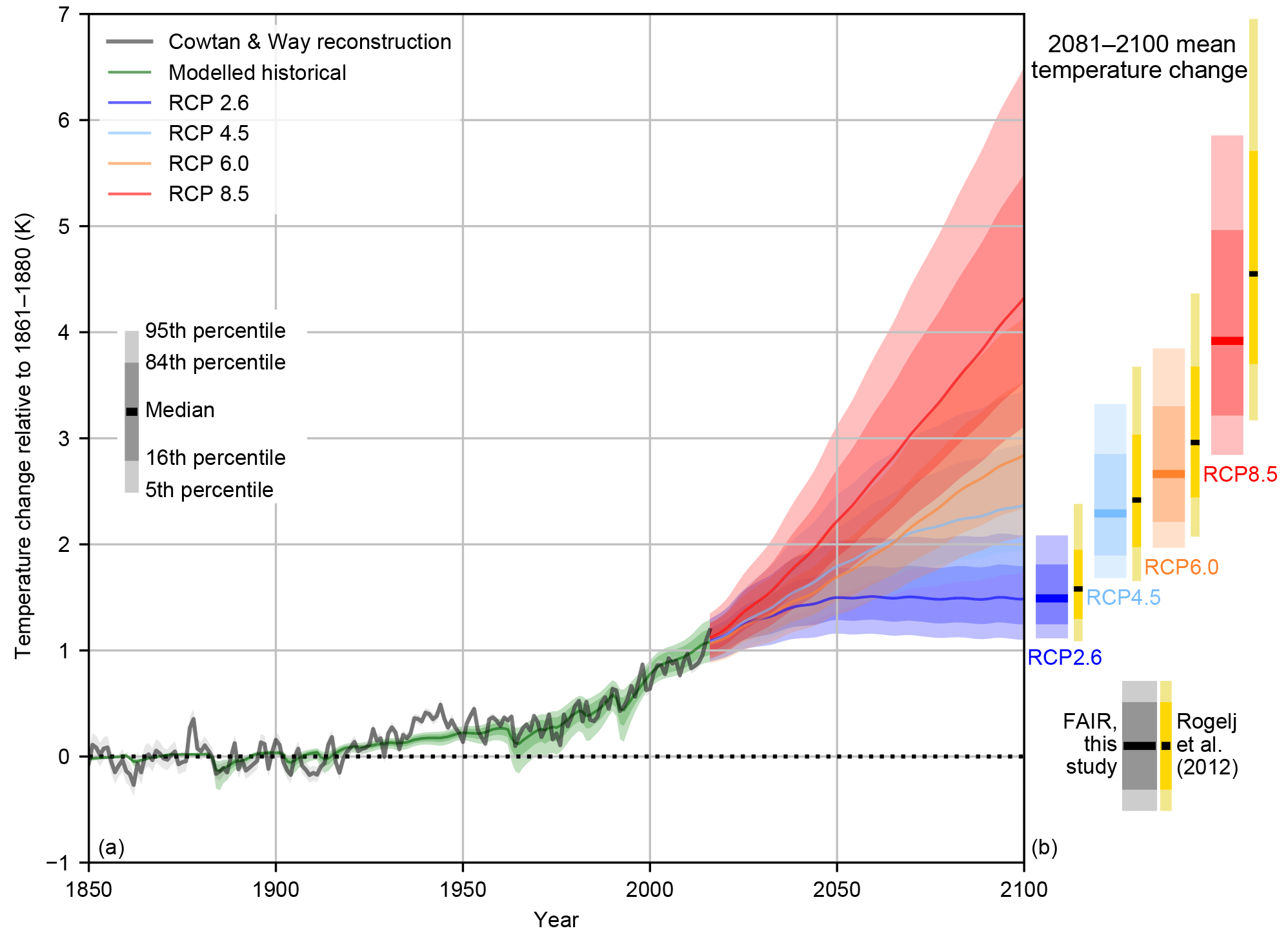
Figure 8 (a) Historical constrained modelled temperature and future probabilistic temperature scenarios from FAIR driven by emissions and forcing from the RCPs for 1850–2100 expressed as temperature change since 1861–1880. Also shown is observed temperature from C&W. (b) Comparison of 2081–2100 mean temperature from FAIR compared to the emission-driven ensemble from MAGICC6 (Rogelj et al., 2012).

4.5 Observed and future temperature changes

Figure 8a shows the transient historical and RCP-projected temperature change for 1850–2100 along with the 2081–2100 median, 1σ (16–84 % range) and 5–95 % credible range for the NROY ensemble (Fig. 8b), (c.f. Rogelj et al., 2012; Collins et al., 2013, Fig. 12.8b). For the RCP scenarios, the median NROY estimates of temperature change for 2081–2100 are 1.49, 2.29, 2.66 and 3.91 K above pre-industrial for RCPs 2.6, 4.5, 6.0 and 8.5 respectively. The median, 1σ and 5–95 % ranges of total temperature change predicted from FAIR are a little lower for RCPs 2.6, 4.5 and 6.0 than those predicted by the emissions-driven MAGICC6 experiments which are reported in AR5 (Rogelj et al., 2012; Meinshausen et al., 2009) and substantially lower for RCP8.5. The RCP8.5 temperature change is lower despite higher 21st-century ERF profiles in FAIR compared to RF in MAGICC. The difference of 0.6 K in the median end-of-century warming in RCP8.5 could be particularly important in policy assessments.

Differences between the models can arise from many sources. The results of Rogelj et al. (2012) are based on best estimates of the ECS∕TCR and radiative forcing from the IPCC Fourth Assessment Report (AR4), whereas we guide FAIR using AR5 forcings. Differences between this study and Rogelj et al. (2012) could be due to differences in the historical radiative forcing time series. The RF over the 1861–1880 to 2005 period, which forms the bulk of the period used to constrain the ensemble to observed temperatures, is 1.72 W m⁻² in Meinshausen et al. (2011b) whereas the ERF differences are 1.98 W m⁻² in AR5 and 1.97 W m⁻² in FAIR over the same period. Therefore, the same observed temperature change would be recreated with a smaller RF in Rogelj et al. (2012) than the corresponding ERF in FAIR, and the same future forcing in MAGICC6 would lead to a higher temperature change than in FAIR. Other differences between the studies include a different selection of ECS and TCR priors in Meinshausen et al. (2009) and Rogelj et al. (2012) (based on AR4 but not substantially different from the CMIP5 models used in this study), a different method of constraining to observed temperatures, and different assumptions regarding the strength of future aerosol and ozone forcing. The sensitivity to some of these assumptions is tested in Sect. 5.

4.6 Transient climate response to emissions

There is an approximately linear relationship between cumulative CO₂ emissions and temperature, independent of the actual emissions pathway taken, provided temperature is still increasing (Allen et al., 2009; Collins et al., 2013). Using this linearity we can diagnose the transient climate response to emissions (TCRE), defined as the change in temperature for a 1000 Gt cumulative emission of carbon.

We show both the TCRE assuming CO₂ forcing alone and the temperature change due to all forcing agents but measured against cumulative carbon emissions (Fig. 9). When including the effect of non-CO₂ forcing on the total temperature change, the temperature response is substantially larger than for CO₂ forcing alone. This indicates that a smaller cumulative CO₂ emission is required to reach the same temperature change and is a result of the total non-CO₂ forcing being positive. This same conclusion was reached in Collins et al. (2013) when assessing a suite of earth system models.

To determine the TCRE we run FAIR in CO₂-only mode. We measure cumulative CO₂ emissions and temperature change since 1870, as this is the date from which reliable estimates of carbon emissions start (Le Quéré et al., 2016) and is also at the centre of the 1861–1880 period used to evaluate temperature changes.

The NROY ensemble in FAIR shows a TCRE of 0.95 to 2.22 K for a cumulative carbon emission of 1000 Gt with a best estimate of 1.39 K. We diagnose TCRE based on the RCP8.5 simulation. The TCRE range from FAIR is within the range of estimates from AR5 (0.8 to 2.5 K, Collins et al., 2013). Towards higher cumulative CO₂ emissions in RCP8.5 the temperature response has a slightly concave shape. The slight (rather than moderate) downward curvature is also present in CMIP5 earth system models, as the increase in airborne fraction of CO₂ with emissions almost cancels out the logarithmic relationship between CO₂ concentration and temperature (Millar et al., 2016).

Figure 9 Transient climate response to CO₂ emissions (TCRE) for FAIR based on RCP8.5 for all forcing (red) and for CO₂-only forcing (black).

4.7 Top of atmosphere energy imbalance

The top of atmosphere energy imbalance N can be diagnosed from (Forster et al., 2013)

$$\begin{array}{}\text{(25)}& N=F-\mathit{\lambda }T,\end{array}$$

where λ is the climate feedback parameter and $\mathit{\lambda }=F_{\mathrm{2}\times }/\text{ECS}$. In Fig. 10 we compare FAIR model outputs from the NROY ensemble under RCP4.5 to observations of the earth's energy imbalance from satellites (Clouds and the Earth's Radiant Energy System; CERES) and from the array of Argo floats (Argo, 2000), which measure ocean temperature which is the largest component of the change in earth's energy budget. Both datasets are taken from Johnson et al. (2016).

For most years from 2001 to 2015, the net energy balance from CERES is within the uncertainty range estimated from the FAIR NROY ensemble. The Argo estimate of N is more variable prior to 2005, after which coverage of the Argo floats saw a large increase (Johnson et al., 2016). From 2005 onwards, all Argo estimates but one fall inside the credible range of FAIR estimates. Both CERES and Argo observations from 2005 onwards are clustered towards the lower half of the credible range from FAIR, which may indicate that ECS over the 2005–2015 period could be towards the lower end of the credible range estimated from the NROY ensemble.

Table 7 Sensitivity in the ECS, TCR and TCRE to variations in the underlying assumptions in the FAIR large ensemble. For the sensitivity experiments the section number in the paper describing the change is given. The “accepted” column details the proportion of the 100 000-member FULL ensemble that satisfied the specified temperature constraint.

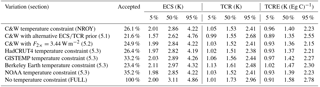
Table 8 Sensitivity in the effective radiative forcing to variations in the underlying assumptions in the FAIR large ensemble.

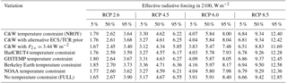
Table 9 Sensitivity in the 2100 temperature change in RCP scenarios to variations in the underlying assumptions in the FAIR large ensemble.

5 Sensitivity to prior distributions and constraints

To determine the robustness of the results of the NROY ensemble, the input assumptions were varied or the ensemble members subjected to a different constraint as described in this section. The results are summarised in Tables 7, 8 and 9.

5.1 Prior distributions of ECS and TCR

The prior distributions of ECS and TCR have a large influence on the posterior distributions attained (Pueyo, 2012). Here we test the dependence of the shape of the posterior distributions of ECS and TCR in the constrained samples on the choice of prior distributions.

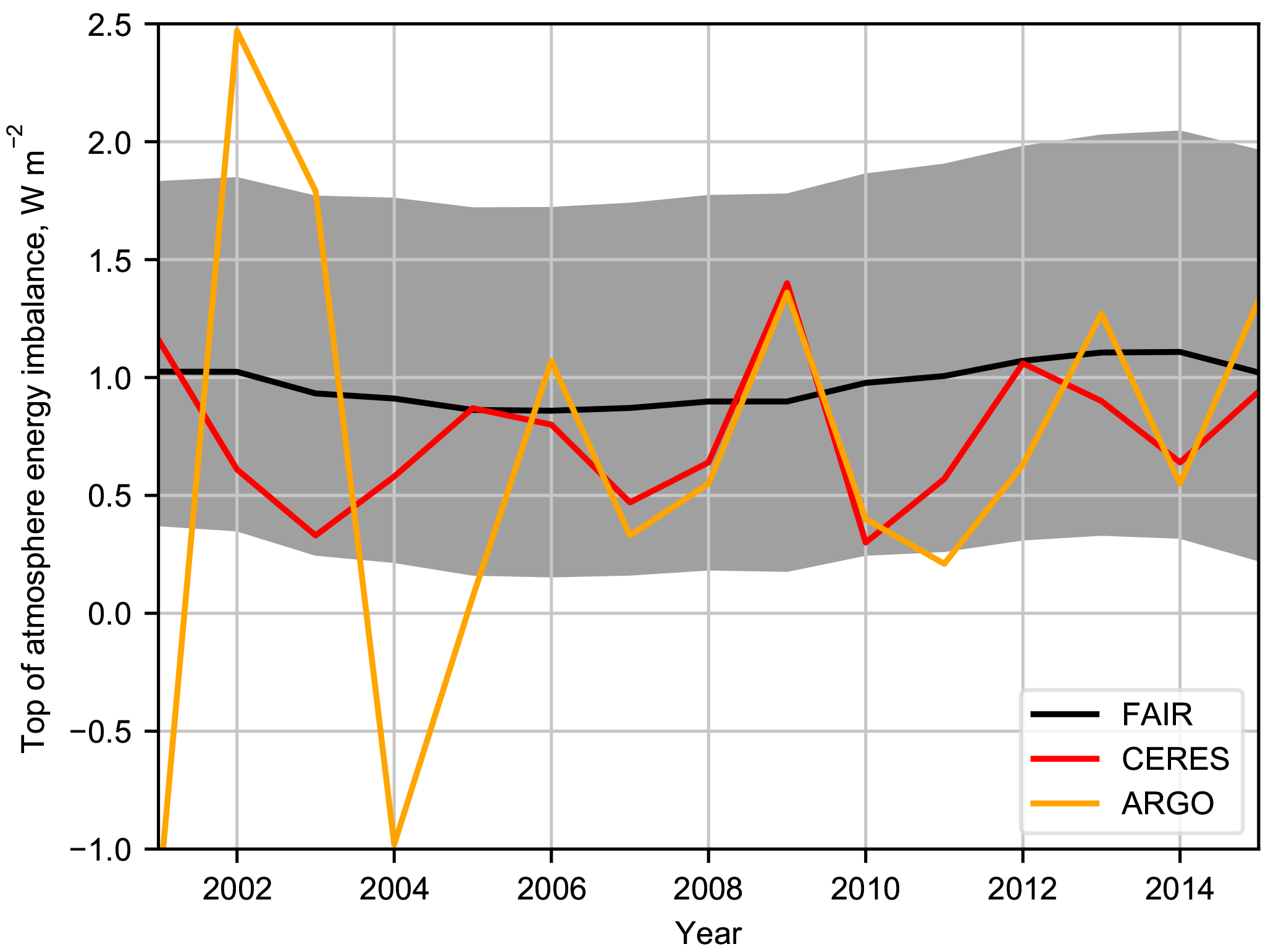
Figure 10 Comparison of earth's energy imbalance N to observations from Argo and CERES, from Johnson et al. (2016).

As the RWF is approximately independent of TCR we use an alternative prior starting with the distributions of TCR and RWF. Noting the analysis of Collins et al. (2013), the likely AR5 range of TCR of 1.0 to 2.5 K is taken to be most probable, with values between 0.5–1.0 K and 2.5–3.5 K possible but unlikely. A trapezoidal distribution in TCR with these limits is constructed, therefore not expressing any prior judgement about the most likely value of TCR within the likely AR5 range. The RWF is sampled from a Gaussian distribution with mean 0.6 and 5–95 % range of 0.45–0.75 following Millar et al. (2017), truncated to fall within the 0.2–1.0 range. These ranges are subjective choices based on evidence from CMIP5 models. The posterior distribution of ECS in particular can be sensitive to the choice of prior distribution (Frame et al., 2005; Pueyo, 2012). Figure S2 shows the alternative prior distributions and the posteriors obtained as a result of constraining to the C&W observed temperatures.

The best estimate and credible range of ERF is very similar to NROY with the alternative prior distributions (Table 8). However, the future temperature projections under the RCPs span a wider range than in NROY (Table 9). This is due to the wider range of ECS and TCR admitted in the posterior distributions (Table 7) using this alternative prior.

5.2 ERF from a doubling of CO₂

The canonical RF value of $F_{\mathrm{2}\times }=\mathrm{3.71}$ W m⁻² may not be applicable when considering all land surface and tropospheric rapid adjustments in the definition of ERF. For CO₂ forcing, rapid adjustments include cloud changes that are not driven by temperature change (Gregory and Webb, 2008) and land surface adjustments consequential to plant stomatal conductance (Doutriaux-Boucher et al., 2009). The mean ERF for a doubling of CO₂ in CMIP5 models was found to be 3.44 W m⁻² (Forster et al., 2013). The simulation is repeated with this new lower ERF value for a doubling of CO₂, with the same uncertainty of 20 %.

It is found that this lower value of F_2× slightly lowers the best estimate and credible range of ECS, TCR and ERF, but the temperature change under the RCP scenarios is higher than in NROY due to non-CO₂ forcings. This behaviour can be analysed with the help of Eq. (25). In equilibrium states, the top of atmosphere (TOA) energy imbalance N=0 and Eq. (25) is rearranged to yield $T=F_{\mathrm{2}\times }/\mathit{\lambda }$. If F_2× is found to take a lower value and ensemble members are constrained to the same observed temperature, then the climate sensitivity 1∕λ must be higher to compensate for this. Therefore, the same positive future non-CO₂ forcing time series will produce higher temperatures in the future.

5.3 Historical temperature constraint

Historical temperatures were also constrained using the HadCRUT4 dataset without infilling (Morice et al., 2012), along with the GISTEMP (Hansen et al., 2010), Berkeley Earth (Berkeley Earth, 2017) and NOAA (Zhang et al., 2017) observational datasets. The linear 1880–2016 trends are 0.91±0.18 K, 0.99±0.22 K, 1.07±0.16 K and 0.93±0.24 K respectively. All datasets, including C&W (0.95±0.17 K), were accessed on 17 October 2017.

We also perform analysis on the FULL dataset, where the input assumptions are guided by CMIP5 models and AR5 uncertainty ranges but no constraint to historical temperature is performed. We show in Tables 7, 8 and 9 that ECS, TCR, TCRE, ERF and temperature change depend slightly on the dataset of constraint, with datasets showing more warming over the historical period also projecting warmer 2100 temperatures under the RCP scenarios. Using the FULL ensemble, however, leads to wide uncertainty bounds and higher median estimates of these diagnosed parameters than using any of the constrained ensembles. Therefore, using a historical temperature constraint rejects parameter combinations that produce larger future temperature changes.

6 Conclusions

We present a simple model, FAIR v1.3, that calculates global temperature change, effective radiative forcing from a variety of drivers and concentrations of greenhouse gases. The emissions-based model is based on the FAIR v1.0 carbon-cycle–climate model with an extension for emissions of non-CO₂ greenhouse gases, ozone precursors and aerosols. This version of FAIR, which is tuned to the effective radiative forcing time series in AR5 over the historical period, provides ERFs that are close to the target radiative forcings from the RCP scenarios in 2100. FAIR was not tuned to emulate the radiative forcing in the MAGICC6 model; however, it closely matches the concentrations of greenhouse gases projected in that model.

Within FAIR, the response of the carbon cycle model can be adjusted via the rate of uptake of carbon by land and ocean processes parameterised as a function of total temperature change and cumulative carbon emissions (iIRF₁₀₀). Emissions and concentrations are converted to effective radiative forcing and the relationship of ERF to temperature change is governed by the TCR, ECS and the efficacy of each of the 13 separate forcing categories considered in the model. The emulation of specific earth system models is therefore possible as discussed by Millar et al. (2017).

Using a correlated joint log-normal prior distribution of ECS and TCR based on CMIP5 models, running a 100 000-member ensemble in FAIR, and keeping only those ensemble members that match the rate of temperature change from 1880–2016 in C&W (the “not ruled out yet” or NROY ensemble), we find the median and 5–95 % credible ranges of ECS and TCR to be 2.86 (2.01 to 4.22) K and 1.53 (1.05 to 2.41) K respectively. The transient climate response to CO₂ emissions (TCRE) is diagnosed from a CO₂-only ensemble and found to be 1.40 (0.96 to 2.23) K (1000 GtC)⁻¹. These ranges are similar to the IPCC likely AR5 ranges for ECS, TCR and TCRE, albeit with tighter credible bounds. The NROY best estimates and ranges are not very sensitive to a lower estimate of the ERF from a doubling of CO₂ or a different observational temperature dataset to constrain the historical temperature change rather than the Cowtan and Way (2014) dataset. They are more sensitive to the prior distribution of ECS and TCR, particularly for the constraint on ECS. All methods of constraint lead to lower median and credible range estimates of ECS, TCR and TCRE than not constraining to temperature at all (the FULL ensemble, with input parameters estimated from the distribution of CMIP5 models and ERF uncertainties based on AR5 estimates).

Our estimate of TCR is not as low as the range derived by Otto et al. (2013) from observational constraints (0.9 to 2.0 K). Similarly our best estimate of ECS is higher than the estimate provided by Gregory and Andrews (2016) of around 2 K using observed sea-surface temperatures and sea ice in two atmosphere-only general circulation models (GCMs). While we cannot absolutely rule out values of ECS greater than 5 K or TCR greater than 2.5 K, this would require a strong present-day aerosol forcing (at least as negative as −1.0 W m⁻²) to balance. Progress towards tightening these upper bounds could therefore be achieved with a better understanding of the present-day aerosol forcing (Stevens et al., 2016).

Temperature changes projected in the NROY ensemble in 2100 are a little lower than those from Rogelj et al. (2012) for the RCP scenarios, except for RCP8.5 where FAIR is 0.6 K lower in the median response. This is due to the lower ensemble estimates of ECS and TCR in NROY and the differences in present-day minus 1850 radiative forcing between AR5/NROY and the RCP radiative forcing in Meinshausen et al. (2011b). Nevertheless, under RCP8.5 the median year 2100 temperature projection is 4.32 K above the pre-industrial in our NROY ensemble, which would have very severe global consequences. Conversely the median estimate for RCP2.6 is 1.48 K, suggesting about a 50 % chance of limiting end-of-century warming to 1.5 K under this pathway.

FAIR is useful for creating large ensembles of future temperature change based on input uncertainties in the carbon cycle parameters and effective radiative forcing strengths. This can be used for instance to assess the impacts of emissions commitment scenarios or committed warming (Ehlert and Zickfeld, 2017) or if a certain category of emissions such as aerosols are increased or decreased in the future. FAIR can be used with integrated assessment models to calculate the social cost of carbon in the presence of non-CO₂ forcing agents. Following the 2015 Paris Agreement and in anticipation of the 2018 IPCC Special Report, the FAIR model can be used to investigate emissions pathways consistent with 1.5 and 2 K total warming limits, including remaining carbon budgets, and give probabilistic indications of the likelihood of these limits being breached.