Optimizing UV Index determination from broadband irradiances

A study was undertaken to improve upon the prognosticative capability of Environment and Climate Change Canada's (ECCC) UV Index forecast model. An aspect of that work, and the topic of this communication, was to investigate the use of the four UV broadband surface irradiance fields generated by ECCC's Global Environmental Multiscale (GEM) numerical prediction model to determine the UV Index.

The basis of the investigation involves the creation of a suite of routines which employ high-spectral-resolution radiative transfer code developed to calculate UV Index fields from GEM forecasts. These routines employ a modified version of the Cloud-J v7.4 radiative transfer model, which integrates GEM output to produce high-spectral-resolution surface irradiance fields. The output generated using the high-resolution radiative transfer code served to verify and calibrate GEM broadband surface irradiances under clear-sky conditions and their use in providing the UV Index. A subsequent comparison of irradiances and UV Index under cloudy conditions was also performed.

Linear correlation agreement of surface irradiances from the two models for each of the two higher UV bands covering 310.70–330.0 and 330.03–400.00 nm is typically greater than 95 % for clear-sky conditions with associated root-mean-square relative errors of 6.4 and 4.0 %. However, underestimations of clear-sky GEM irradiances were found on the order of ∼ 30–50 % for the 294.12–310.70 nm band and by a factor of ∼ 30 for the 280.11–294.12 nm band. This underestimation can be significant for UV Index determination but would not impact weather forecasting. Corresponding empirical adjustments were applied to the broadband irradiances now giving a correlation coefficient of unity. From these, a least-squares fitting was derived for the calculation of the UV Index. The resultant differences in UV indices from the high-spectral-resolution irradiances and the resultant GEM broadband irradiances are typically within 0.2–0.3 with a root-mean-square relative error in the scatter of ∼ 6.6 % for clear-sky conditions. Similar results are reproduced under cloudy conditions with light to moderate clouds, with a relative error comparable to the clear-sky counterpart; under strong attenuation due to clouds, a substantial increase in the root-mean-square relative error of up to 35 % is observed due to differing cloud radiative transfer models.

1 Introduction

Throughout the late 1980s and early 1990s, extensive atmospheric studies in the polar regions of the planet revealed that stratospheric ozone (O₃) concentrations were being depleted due to a variety of O₃-destroying catalytic cycles driven by photochemical reactions liberating chlorine (Cl) and bromine (Br) atoms from chlorofluorocarbon (CFC) and hydrofluorocarbon (HCFC) molecules emitted into the atmosphere as airborne anthropogenic pollutants (Rowland, 1996).

Ozone is an important atmospheric absorber of energetic short-wavelength radiation emitted by the Sun. Most critically, O₃ is the primary absorber of ultraviolet (UV) radiation, which has wide-ranging implications for the health of the biosphere: both on a molecular level with the potential of damaging the cellular DNA of individual organisms (Ravanat et al., 2001) and the destabilization of entire biogeochemical cycles within a biome (Zepp et al., 1998).

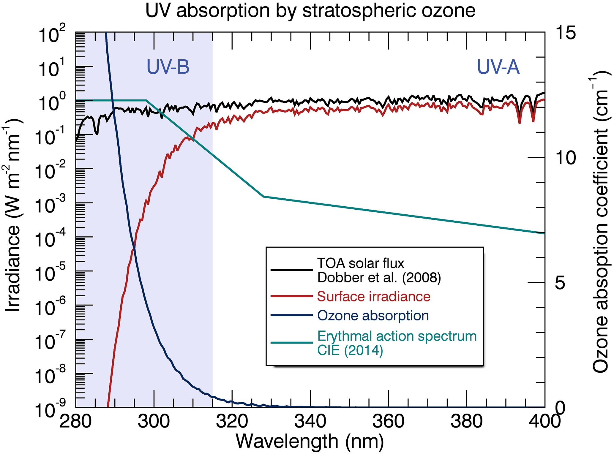
Figure 1 Sample UV irradiance spectrum at the Earth's surface on a clear summer day (averaged and sampled over 0.5 nm intervals). Stratospheric (O₃) is the primary species which serves to absorb UV radiation in the atmosphere (blue curve). The Huggins–Hartley band system of O₃ attenuates the radiative flux (black curve) by several orders of magnitude in the UV-B region. The product of the absorption cross section and the top-of-atmosphere flux gives the resultant incoming irradiance at the surface (red curve). The erythemal action spectrum (green curve) demonstrates the increasing susceptibility of human skin to epidermal damage (erythema).

UV radiation is categorized into three broadband regions which are defined as UV-A (315–400 nm), UV-B (280–315 nm), and UV-C (100–280 nm). Molecular species in the Earth's atmosphere absorb very little of the longer-wavelength UV-A radiation, as it reaches the surface with a minor net difference (mainly due to scattering) in the radiative flux from the top of the atmosphere. UV-B radiation is partially transmitted through the atmosphere and is primarily absorbed by O₃ (Huggins–Hartley band system). The Huggins–Hartley system (∼ 200–360 nm) of O₃ and the Hopfield and Schumann–Runge systems (∼ 70–200 nm) of molecular oxygen (O₂) serve to absorb all UV-C radiation, which is impeded from reaching the top of the troposphere. This absorption occurs primarily in the ozone layer, a thin band of O₃ contained within the stratosphere where the peak molecular number density of O₃ is located ∼ 20–30 km above sea level. Figure 1 demonstrates how the absorption by ozone increases rapidly with decreasing wavelength in the UV-B region, causing surface irradiances to fall off sharply with decreasing wavelength.

At progressively shorter wavelengths of UV light, increasingly energetic photons become subsequently more and more damaging to biological species, including humans. Studies were conducted as early as the 1930s to quantify the damage done to human skin by UV radiation. It had been well known for quite some time that UV-A and UV-B radiation are harmful to unicellular organisms, the surface cells of plants and animals, and to the health of the more photosensitive population. Increased photosensitivity in people can be caused by a number factors, the most common cause is due to having minimal skin pigmentation (melanin), which provides a natural barrier to the Sun's UV rays. Certain immune system ailments such as solar urticaria can cause hypersensitive allergic reactions to minimal exposures of UV radiation causing hives, rashes, and blistering. Photosensitivity is often associated with the use of certain medications, including some non-steroidal anti-inflammatory drugs and painkillers, tranquillizers, oral anti-diabetics, antibiotics, and antidepressants (http://www.who.int/uv/faq/uvhealtfac/en/).

Colblentz and Stair (1934) sought to obtain measurements of the spectral erythemic reaction (reddening) of untanned human skin exposed to UV light. In essence, this was one of the first recordings of a UV erythemal action spectrum, where an action spectrum for a particular biological effect expresses the effectiveness of radiation at each wavelength as a fraction of the effectiveness at a certain standard wavelength – in this case, the tolerance of human skin to UV radiation. Today, research has revealed that humans are susceptible to much more than sunburns when exposed to UV rays. Prolonged exposure can lead to the premature aging of the skin, suppression of the immune system, eye damage including the development of corneal photokeratitis and cataracts, and skin cancer (melanoma). The contemporary action spectrum adopted by most international organizations is the CIE (Commission Internationale de l'Éclairage, International Commission on Illumination) action spectrum (CIE Technical Report, 2014). The CIE standard spectrum, Eq. (1), is based on the action spectrum originally developed by McKinlay and Diffey (1987), which was constructed by re-normalizing the data points and modifying the piecewise function to avoid having overlapping wavelength intervals (Webb et al., 2011).

$$\begin{array}{}\text{(1)}& \text{EAS}\left(\mathit{\lambda }\right)=\left\{\begin{array}{ll}\mathrm{1.0}& \mathrm{250}\le \mathit{\lambda }\le \mathrm{298}\\ {\mathrm{10}}^{\mathrm{0.094}(\mathrm{298}-\mathit{\lambda })}& \mathrm{298}<\mathit{\lambda }\le \mathrm{328}\\ {\mathrm{10}}^{\mathrm{0.015}(\mathrm{140}-\mathit{\lambda })}& \mathrm{328}<\mathit{\lambda }\le \mathrm{400}\end{array}\left[\mathit{\lambda }\text{ nm}\right]\right.\end{array}$$

The UV Index was developed as an erythemally weighted representation of the total surface flux of UV radiation in the biologically active range of 280–400 nm (CIE Technical Report, 2014; Fioletov et al., 1997; Allaart et al., 2004; Fioletov et al., 2010; Moshammer et al., 2016); the range below ∼ 280–290 nm can be excluded as its contribution is negligible. It was conceived to produce a simplified scale which reports the relative strength of the Sun's UV radiation, and to inform the public of the Sun protection actions that should be taken as a precaution if they are to be exposed to the Sun's rays for extended periods of time.

To determine the UV Index from high-spectral-resolution irradiances, an effective spectral curve is calculated from the product of the erythemal action spectrum and the surface irradiance (Fig. 2). This effective curve, the weighted UV irradiance, is then integrated over the spectral range representing UV-A and UV-B (280–400 nm) to produce the UV Index (see Eq. 2). A scaling factor of (25 mW m⁻²)^-1 is implemented to provide a convenient set of numerical values, normally ranging from 0 to 11. In extreme cases, values of > 11 can be reached and are typically recorded in the tropics where the solar zenith angle and the total column ozone are small. Extreme values are also recorded at high elevations where the atmospheric optical path is shortened, resulting in a reduced attenuation of actinic fluxes and consequently producing increased surface irradiances.

$$\begin{array}{}\text{(2)}& \text{UVI}={\displaystyle \frac{\mathrm{1}}{\mathrm{25}\mathrm{mW}{\mathrm{m}}^{-\mathrm{2}}}}\underset{\mathrm{280}\mathrm{nm}}{\overset{\mathrm{400}\mathrm{nm}}{\int }}I\left(\mathit{\lambda }\right)\cdot \text{EAS}\left(\mathit{\lambda }\right)\mathrm{d}\mathit{\lambda }\end{array}$$

Amidst mounting concerns arising in the late 1980s from the escalating depletion of stratospheric O₃ due to CFCs, and the subsequent increases in the surface irradiances of UV radiation (Crutzen, 1992), Environment and Climate Change Canada began providing daily UV Index forecasts as of 1992 (Burrows et al., 1994). Since its inception in 1992, the UV Index has been adopted worldwide as a standard indicator to characterize solar UV intensity at the Earth's surface (Fioletov et al., 2010) and serves to inform the public about the strength of the Sun's UV radiation and the adequate sun protection actions recommended to avoid excessive exposure to UV radiation (WHO Report, 2002; CIE Technical Report, 2014). The UV Index was officially adopted as the method of reporting surface UV irradiances by the World Meteorological Organization (WMO) and World Health Organization (WHO) in 1994.

At present, the UV Index determination for the ECCC forecast system relies on a statistically derived weather-based computation of the total column ozone field, adjustments using total column measurements of the Canadian Brewer network, and empirical conversions to the UV Index accounting for the solar zenith angle, cloud conditions, surface altitude, and snow cover. A recently undertaken study toward improving the UV Index forecast system makes direct use of ozone data assimilation, ozone model forecasts, and model UV irradiance forecasts for both clear-sky and cloudy conditions as carried out in some capacity at other forecast centres (e.g., NCEP/NOAA, KNMI, and ECMWF). A summary of UV Index forecasting practices conducted by various governmental organizations worldwide were compiled by Long (2003); a more recently updated overview of UV measurement stations and monitoring networks in Europe was reported by Schmalwieser et al. (2017).

This current study is part of a multi-faceted project which seeks to include having a UV Index forecasting package more tightly integrated into the current weather (and air quality) forecasting system and increasing the array of UV Index products available from ECCC to Canadians, such as daytime variation, longer forecasts, and continental and regional maps. The ECCC Global Environmental Multiscale (GEM) numerical weather prediction model described by Charron et al. (2012), and the references therein, provides four broadband irradiances shown in Fig. 2 covering the UV spectrum in the range of 280–400 nm, which can be calculated using three-dimensional prognostic ozone fields. The work presented in this communication consists of investigating and optimizing the calculation of the UV Index from these broadband irradiances, with focus on clear-sky conditions, for minimizing computational cost and processing time. This is carried out through comparisons of the UV Index and broadband irradiances produced from GEM to those calculated using the Cloud-J radiative transfer model (Prather, 2015), which has been adapted to provide high-resolution irradiance spectra at the Earth's surface.

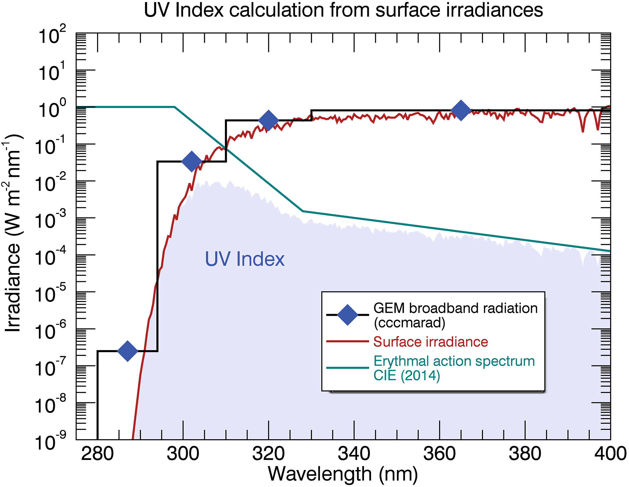
Figure 2 The UV Index is defined as the integral of the erythemally weighted irradiance spectrum (shaded region), produced from the product of the surface irradiance (red curve; see Fig. 1) and the erythemal action spectrum (green curve), over the UV-A and UV-B spectral ranges. The result is then multiplied by a scaling factor (25 mW m⁻²)^-1 to create a numerically convenient value for the index. Also depicted are the corresponding irradiances for the GEM broadbands divided by their respective bandwidths.

The following subsections provide some background on the GEM-based weather forecast system, the Cloud-J radiative transfer model, and their products. Section 2 describes the general methodology and the related fitting approaches applied in Sect. 3 to investigate and optimize the calculation of the UV Index from the broadband irradiances through the use of high-resolution spectral irradiance simulations for clear-sky conditions. While a specific optimization under cloudy conditions is not performed due to differing cloud radiative transfer models, comparisons for both clear and cloudy conditions are presented and fully discussed in Sect. 3. Conclusions are provided in Sect. 4.

1.1 GEM with LINOZ

The irradiance fields calculated by GEM use the CCCmarad radiative transfer model. CCCmarad is an in-house radiation scheme based on a modified version of the Canadian Centre for Climate Modelling and Analysis (CCCma) atmospheric general circulation model (Scinocca et al., 2008), which uses a correlated-k distribution method for gaseous transmission detailed by Li and Barker (2005) and von Salzen et al. (2013). The Li and Barker (2005) radiation scheme has four wave number intervals for the shortwave and nine intervals for the longwave. The visible and UV portion of the shortwave is further subdivided into nine sub-bands. The four sub-bands of relevance to the calculation of the UV Index cover the following spectral ranges: 280.11–294.12, 294.12–310.70, 310.70–330.03, and 330.03–400.00 nm. For convenience, the remainder of the text will instead refer to the integer values of 280, 294, 311, and 400 nm. The irradiances of the sub-bands, i.e., the broadband irradiances, consist of direct and diffuse components, which are available in addition to their sum. This paper involves use of all three irradiance terms of these four sub-bands. It will separately consider the clear-sky and all-sky cases in the calculation of the irradiances as well, with all-sky conditions implying the possible presence of clouds.

The GEM dynamical core is described in Girard et al. (2014), while basic descriptions of the physical parameterizations and detailed references can be found in Zadra et al. (2014a, b). Model runs were performed using a 7.5 min time step for a uniform 1024 × 800 longitude–latitude grid (0.352^∘ × 0.225^∘) and a Charney–Phillips vertically staggered grid with 80 thermodynamic levels extending from the near surface (at η=1) to ∼ 0.1 mbar (η≈0.0001). The analyses, serving as initial conditions for providing the forecasts used in this study, are a composite of the already available ECCC weather analysis and separately generated ozone analyses. The GEM forecast products used as input for the simulations performed with Cloud-J are detailed in Sect. 2.1.

Prognostic ozone is solved with a linearized photochemistry scheme called LINOZ (McLinden et al., 2000), which was implemented online within the GEM NWP model (de Grandpré et al., 2016). For this work, the ozone analyses stem from assimilation of total column ozone data obtained from the National Environmental Satellite, Data, and Information Service (NESDIS/NOAA) for the Global Ozone Monitoring Experiment-2 (GOME-2) instruments of the MetOp-A and MetOp-B satellites (Callies et al., 2000; Munro et al., 2006) . Assimilations were performed with the incremental three-dimensional variational approach with the first guess at appropriate time (FGAT; Fisher and Andersson, 2001) using elements of the system described in Charron et al. (2012), and the references therein, adapted for chemical data assimilation.

For the treatment of cloud, GEM employs a prognostic total cloud water variable with a bulk-microphysics scheme for non-convective clouds. The radiative transfer impact from clouds is primarily dictated by the liquid and ice water mixing ratios (LWCR and IWCR) and cloud fraction (CLDR). Fractional cloudiness is based on a relative humidity threshold, which varies in the vertical. Individual cloud layers are assumed to overlap in the vertical using a maximum random cloud overlap (Sundqvist et al., 1989; Paquin-Ricard et al., 2010).

The GEM model currently does not assimilate aerosol measurement data. The radiative effects associated with background aerosols are based on a climatology produced by Toon and Pollack (1976). This climatology specifies maximum aerosol loading at the Equator and a decrease toward the poles, with different values for continents and oceans. These distributions also include a latitudinal gradient. Aerosols are assumed only to affect the solar absorption properties of the clear-sky atmosphere (Markovic et al., 2008).

1.2 Cloud-J

Cloud-J, a recent release of the Fast-J program (Wild et al., 2000; Bian and Prather, 2002), is a multi-scattering, eight-stream, radiative transfer model for solar radiation (Prather, 2015) developed for integration into three-dimensional chemical transport models to calculate photolysis rates (J values) in the atmosphere. The version of the program used for this work is Cloud-J v7.4. The program is developed and maintained by Michael Prather in the Department of Earth System Science at the University of California, Irvine (http://www.ess.uci.edu/group/prather/scholar_software/cloud-j, last access: 23 March 2018).

To calculate photolysis rates, the standard Cloud-J code uses 18 interpolated wavelength bins covering a spectral range of 187–599 nm. The integrated radiative transfer model uses a plane-parallel atmosphere assumption and a full scattering phase function. Rayleigh and isotropic scattering are taken into consideration. Numerous cloud types and aerosol species of varying sizes are accounted for in the calculations by making use of look-up tables containing the scattering functions for water droplet size, ice crystals of various phases, dust, absorbing soot (black carbon), stratospheric sulfates (background and volcanic), and water haze at 0.1 and 0.4 µm. Optical depth properties include extinction optical depth, single scatter albedo, and a scattering phase function.

Cloud-J provides numerous options for the treatment of clouds in its radiative transfer calculations. Option 1 is the calculation for clear-sky conditions. Options 2 and 3 are variations of the direct use of the cloud water content, which employs cloud fraction and separate liquid and ice water paths. The remaining five options (4–8) employ different variations in the correlated, overlapping cloud scheme. The approach seeks to represent the fractional cloud cover in the model layers through the calculation of numerous independent cloud atmospheres (ICAs), where each ICA would be either 100 % cloudy or clear in each cell of the cloud model layer. This fractional cloud-overlap model serves to determine the layer structure, weighting, and number of ICAs that best represent the actual cloud distribution in the model layers.

2 Methodology

Given the availability of realistic three-dimensional prognostic ozone to the GEM numerical weather prediction model through the LINOZ linearized ozone model and ozone data assimilation, it was proposed to make direct use of the four GEM model UV broadband irradiances at the Earth's surface to calculate the UV Index. The Cloud-J radiative transfer model was adapted to provide high-spectral-resolution surface irradiances in the UV spectral range, 280–400 nm. The high-resolution output is used to evaluate the GEM broadband irradiances for clear-sky conditions and to optimize the determination of the UV Index using these coarse-resolution spectral broadbands. A comparison of results from the two models under cloudy conditions is also performed in Sect. 3.

To perform the optimization of the GEM broadband irradiances, the desired output from Cloud-J is twofold.

1. Sets of Cloud-J broadband irradiances are generated by integrating portions of the high-resolution irradiance spectra to produce simulated versions of the four GEM UV broadbands covering 280–294, 294–311, 311–330, and 330–400 nm.

2. A global UV Index field is produced by integrating the erythemally weighted high-resolution irradiance spectra over the 280–400 nm spectral range, Eq. (2).

Simulated broadband irradiances are generated for comparison with the GEM broadband irradiances and, as needed, used to create sets of scaling functions to calibrate the GEM values to the Cloud-J output. The scaled GEM broadband irradiances are then weighted accordingly such that the global UV Index field produced using the GEM broadband irradiances emulates the high-resolution UV Index field calculated from Cloud-J. Two different approaches were implemented to calculate the UV Index from the resultant GEM broadband surface irradiances. A least-squares fitting was employed in both cases to optimize the weighting under clear-sky conditions using the UV Index field produced from the high-resolution Cloud-J spectra as a reference.

The following subsections briefly describe the application of GEM products and the Cloud-J model to ultimately evaluate and optimize the UV Index determination from the broadband irradiances.

2.1 Calculation of high-spectral-resolution irradiances

Originally designed to calculate tropospheric and stratospheric photolysis rates in 3-D global models, the Cloud-J program was adapted to input three-dimensional fields from the GEM model and output direct and diffuse, high-spectral-resolution surface irradiances instead of mean photolytic intensities. The resultant surface spectral irradiances are, in turn, used to calculate UV Index fields.

To produce the high-spectral-resolution output for UV Index calculations, the number of wavelength bins was increased to 241 with 0.5 nm intervals over the 280–400 nm spectral range. Having augmented the number of wavelength bins to perform the high-resolution calculations, additional spectroscopic data were required for integration into Cloud-J. These spectral parameters were interpolated onto a 0.5 nm resolution grid and reformatted for reading into the program along with the GEM model forecasts. The spectral data incorporated into Cloud-J include

• a set of UV–visible temperature–pressure absorption cross sections for O₃ obtained from the GEISA spectroscopic database (Jacquinet-Husson et al., 2008);

• an Earth surface reflectance climatology from 5 years (2005–2009) of OMI data (Kleipool et al., 2008) (surface reflectivities are provided as monthly averages for 23 wavelength channels and a 328–499 nm range, on a 0.5^∘ × 0.5^∘ grid);

• a high-resolution, top-of-atmosphere (TOA) solar flux spectrum between 250 and 550 nm (Dobber et al., 2008) (provided by Quintus Kleipool of the Royal Netherlands Meteorological Institute, the reference spectrum was created to calibrate and validate the Ozone Monitoring Instrument, OMI);

• Rayleigh scattering parameters calculated using the methodology detailed in a publication by Chance and Spurr (1997).

The O₃ cross sections obtained from the GEISA database (http://cds-espri.ipsl.upmc.fr/etherTypo/index.php?id=950&L=1, last access: 23 March 2018) were recorded by Voight et al. (2001) on a Bruker IFS 120HR Fourier-transform spectrometer at a spectral resolution of 5.0 cm⁻¹. The measurements were performed as a follow up to the cross-sectional data initially recorded by Burrows et al. (1999) on the GOME-FM instrument. The new data sets recorded by Voight et al. (2001) offer precise reference spectra where the spectral accuracy of the data is better than 0.1 cm⁻¹ (∼ 0.5 pm at 230 nm and ∼ 7.2 pm at 850 nm), which was validated by recording visible absorption spectra of gaseous diatomic iodide (I₂) in a reference cell using the same experimental set-up. The agreement between observed and modelled data was determined to be 1 % and better within the 255–310 nm region. Sets of O₃ absorption spectra were recorded using total pressures of 100 and 1000 mbar at five different temperatures ranging from 203 to 293 K. The spectra in the UV range at 100 and 1000 mbar are nearly identical to larger differences at higher wave numbers. Three O₃ absorption spectra from this data set were used for incorporation into Cloud-J (1000 mbar at 293 K and 100 mbar at 246 and 223 K). The selection of the three spectra was based on consideration of the typical temperature distribution as a function of pressure.

In addition to the O₃ temperature cross sections, the O¹D quantum yields associated with ozone photolysis were also required by the Cloud-J radiative transfer model. Values for the quantum yields were calculated using the prescribed method outlined by Matsumi et al. (2002) for the same three temperatures associated with the GEISA O₃ cross sections.

The albedo data were interpolated from their native grid onto the 1024 × 800 GEM global grid. A linear interpolation was then performed on the data from the 23 re-gridded wavelength channels to obtain the intermediate albedo global fields corresponding to 0.5 nm intervals over the 328–400 nm spectral range to be subsequently used in the high-resolution irradiance calculations. Albedo values for the bins corresponding to the missing wavelength range of 280–328 nm were obtained by linearly interpolating the data between the 328 nm OMI channel and the UV-B values published by Chadyšien and Girgždys (2008). According to the experimental data reported in Table 2 of Chadyšien and Girgždys (2008), snow and/or ice are the primary reflectors of UV-A and UV-B radiation, where surface reflectivity for these spectral regions is 94 and 88 % respectively, representing a drop in reflectivity of 6.38 % in the shorter wavelength region. To emulate the experimental data, the reflectivities for the 328 nm OMI channel were linearly reduced by 6.38 % over the 280–328 nm spectral range.

The OMI solar reference spectrum produced by Dobber et al. (2008) was used to provide the TOA solar flux values required for the high-resolution irradiance calculations performed by Cloud-J. Currently, there are no high-resolution solar spectra that cover the UV-A and UV-B wavelength ranges. Most UV–vis TOA spectra are pieced together from different sources in order to provide a continuous, unbroken spectrum. The OMI reference spectrum was created to validate the radiometric calibration of OMI measurements and to monitor potential optical degradation of the instrument. Also a combined spectrum, it was produced by employing the approach used by Chance and Spurr (1997). It merges the balloon spectrum of Hall and Anderson (1991), which covers a shortwave UV region between 200 and 310 nm, with a ground-based spectrum obtained from the McMath–Pierce solar telescope at Kitt Peak National Observatory (Kurucz et al., 1984). The broadband Kitt Peak spectrum covers a spectral range of 296–1200 nm. The final derived spectrum is at 0.01 nm sampling and at 0.025 nm resolution.

This spectrum was chosen for use in this work because the OMI composite spectrum uses high-resolution (0.01 nm) UV measurements made in the stratosphere from a balloon at ∼ 40 km in altitude (Hall and Anderson, 1991) to avoid affects of the strong atmospheric absorption below 300 nm (Dobber et al., 2008). The solar reference spectrum produced by Thuillier et al. (2003) was also considered since it is composed of measurements made from the SOLSPEC and SOSP satellite instruments (Thuillier et al., 1998, 2003) with a resolution of 1 nm. With both spectra being similar, the former was selected due to its higher spectral resolution even though the resolution of the latter is only a factor of 2 coarser than our simulation resolution. A moving boxcar averaging window covering ±0.25 nm about sampling points at intervals of 0.5 nm was applied to the OMI composite spectrum to generate the simulation spectrum.

Consideration was also given to high-resolution spectra based on accurate models of the Sun using the Kurucz et al. (1984) spectrum, such as those by Chance and Spurr (1997) and Chance and Kurucz (2010), which provide excellent spectral range, sampling, and resolution. These spectra unfortunately neglect optimization in the UV-B region for radiometric accuracy. The SAO96 and re-calibrated SAO96 (SAO2010) reference spectra described by Chance and Kurucz (2010) both utilize the original Kurucz et al. (1984) Kitt Peak spectrum for UV-B, where O₃ structure was not fully removed. Chance and Spurr (1997) reported that efforts were focused on intensity calibration of the wavelength range where most application to satellite measurements is performed. Intensities for portions of the spectrum shortward of 305 nm may be in substantial disagreement, by as much as 20 %, with both Dobber et al. (2008) and Thuillier et al. (2003). These spectra were deemed unsuitable for use in the calculation of the UV Index.

It should be noted that the solar spectrum used in this work is representative of a yearly average value of the Earth's TOA flux. Changes in the Earth–Sun distance and associated solar fluxes during the Earth's annual cycle are taken into account and are corrected for by Cloud-J in the high-resolution simulations.

The input atmospheric conditions provided to Cloud-J for this study consist of a set of 6 h forecasts from the GEM model output for the dates of 23–29 August 2015, at 18:00 UTC with daytime over North America. The GEM fields provided as input are surface pressure, and the three-dimensional fields of temperature, pressure (derived from the vertical coordinate and surface pressure), ozone, specific humidity (converted to relative humidity), LWCR and IWCR, and CLDR. For the all-sky conditions, the parameters LWCR, IWCR, and CLDR determine the liquid and ice water partial column amounts (g m⁻²) of each model layer in the presence of clouds.

Cloud-J was run individually for each day during the period of 23–29 August 2015 to produce irradiance fields representing the direct, diffuse, and total surface flux under both clear-sky and all-sky conditions. Weekly (7-day) averages of the direct, diffuse, and total spectral irradiances served as reference spectra in the least-squares minimization for evaluation and adjustment of GEM broadband irradiances, with individual forecast values used in the scatter plot comparisons. While the choice of 7 days was arbitrary as fewer or more days could also have been selected, the averaging was performed for computational efficiency in the minimization. The UV indices produced with Eq. (2) from the weekly averages of total spectral irradiances served as reference in optimizing broadband irradiances based on UV Index estimation models. The UV Index field from the clear-sky weekly averages is shown in Fig. 3.

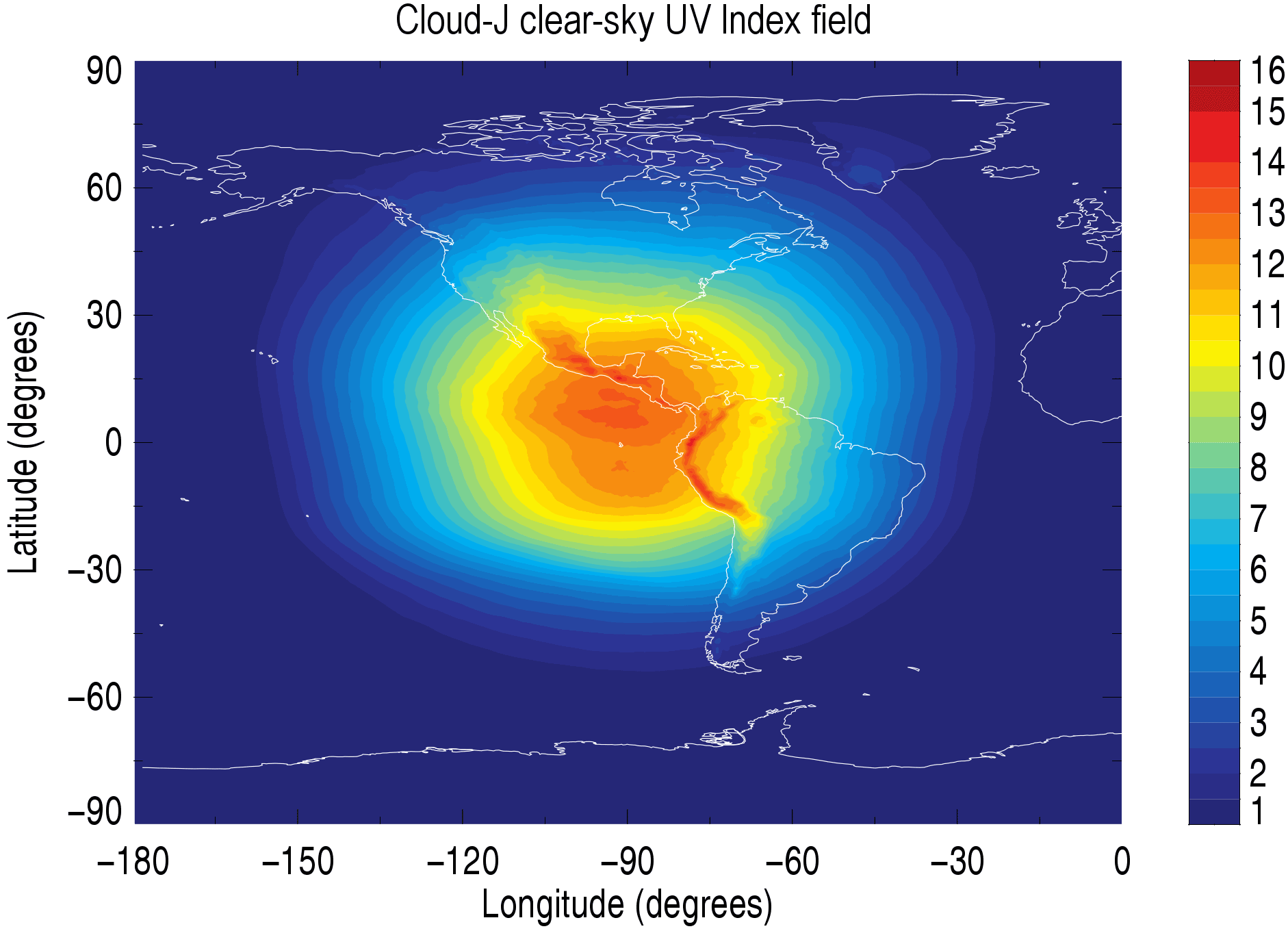
Figure 3 Cloud-J clear-sky UV Index field produced using GEM 6h forecast data with the OMI and GEISA spectral parameters detailed in Sect. 2.1. The UV Index field was generated from a 7-day average of spectral irradiances produced from 23 to 29 August 2015 at 18:00 UTC.

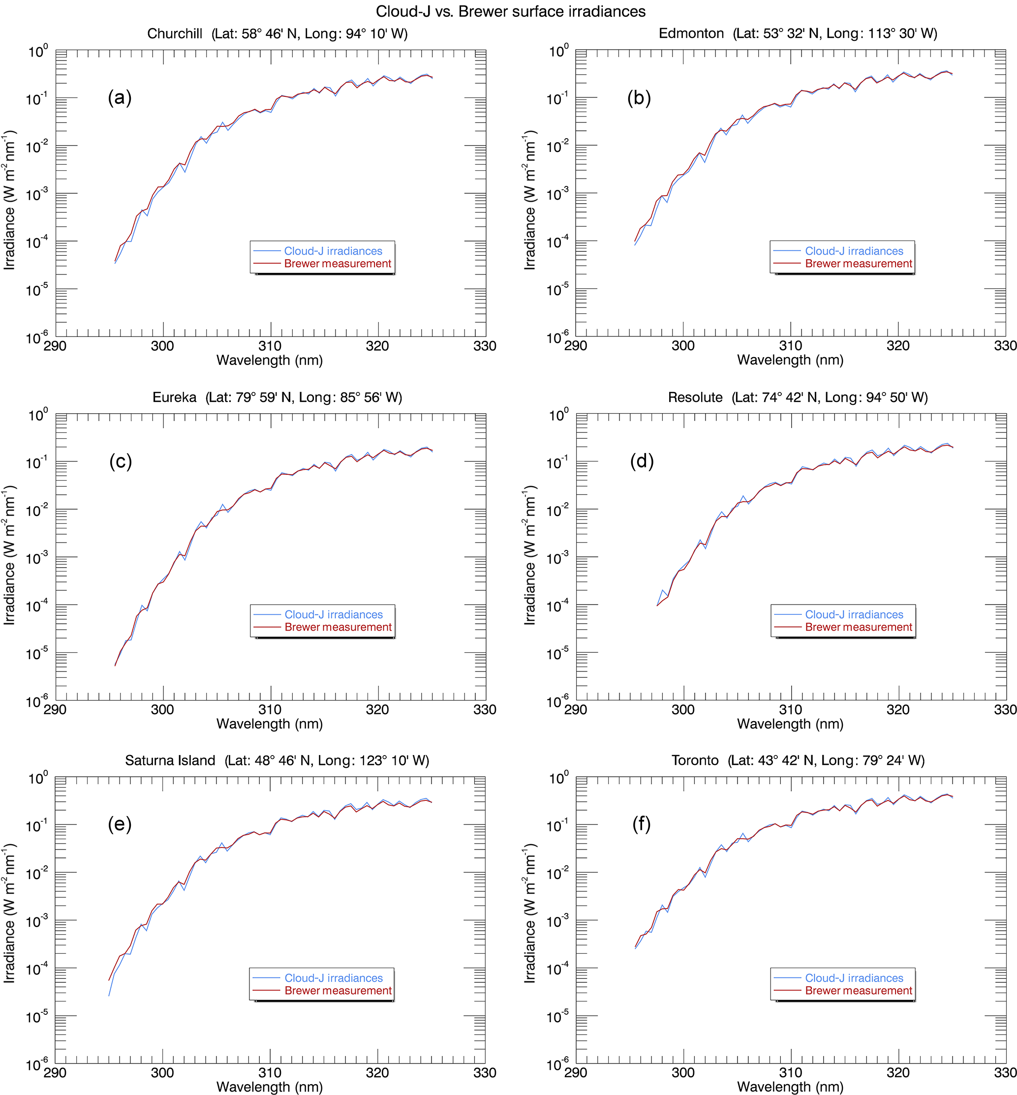
Figure 4 Cloud-J clear-sky surface irradiances compared to in situ Brewer measurements obtained from six measurement stations belonging to ECCC's ozone monitoring network. Plotted are 5-day averages for 18:00 UTC of Brewer spectral irradiances (red curve) and the associated Cloud-J irradiances (light blue). The Cloud-J irradiances shown here were calculated with the Dobber et al. (2008) TOA spectrum averaged over 0.5 nm intervals with a sampling resolution also of 0.5 nm.

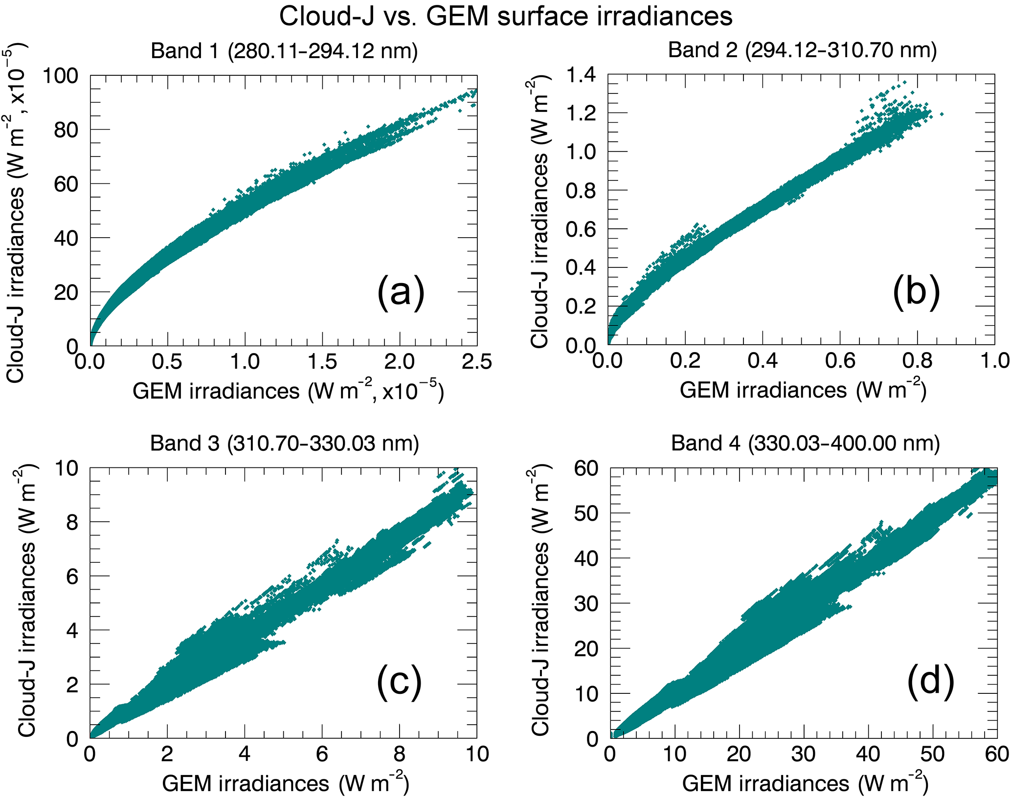
Figure 5 Correlation of GEM and Cloud-J total surface irradiances for clear-sky conditions. The GEM UV broadband irradiances are compared to simulated broadband irradiances produced by integrating the high-resolution Cloud-J output over the same spectral regions. Presented are the individual 7-day irradiance contributions from 23 to 29 August 2015.

2.2 Comparison to ground-based clear-sky irradiances

In addition to measuring total column ozone, Brewer spectrophotometers provide ground-based measurements of the UV spectrum in the range of 290–325 nm with a full width at half maximum of about 0.58 nm and a sampling interval of 0.5 nm. The data processing scheme used to generate spectral irradiances at each 0.5 nm interval, which includes calibration and corrections for various factors, is described in the work detailed by Kerr (2010) and the references within. A sample inter-comparison of three Brewer instruments by Thompson et al. (1997) (see Kerr, 2010, for other inter-comparison sources) showed relative overall differences between instruments within 6 % with an average of 3 % for wavelengths longer than 300 nm; uncertainties are larger at shorter wavelengths.

Cloud-J clear-sky surface UV irradiances were compared to Brewer spectra obtained from six different measurement stations belonging to ECCC's ozone monitoring network and identified to be under clear-sky to optically thin cloud conditions. The applied TOA solar spectrum used here for the Cloud-J simulations, as well as for optimizing use of the GEM broadband irradiances in UV Index calculations, has the same sampling interval of 0.5 nm as the Brewer measurements and a similar effective resolution of 0.5 nm. For the latter, a boxcar averaging window was applied instead of the approximately triangular-shaped Brewer slit function. Figure 4 depicts 5-day averages of Brewer measurements taken at 18:00 UTC on random days in the months of July and August of 2015 and the equivalent counterpart irradiance spectra calculated from Cloud-J. The locations were chosen to provide in situ measurements for different solar zenith angles in addition to varying geographic locations to evaluate the level of agreement between the Cloud-J model application and the Brewer spectra. Only 5-day averages were used, partly due to the limited number of coincident Brewer measurements made during the July–August 2015 period which met the selection criteria for the comparative analysis. Brewer measurements not only had to have been made under clear-sky or near-clear-sky conditions but also had to have been recorded within ∼ 2 min local time of the analogous 18:00 UTC model data.

The Cloud-J derived spectral irradiance curves largely follow those recorded by the Brewer spectrophotometers. The differences between the sets of curves give an overall root-mean-square relative error between the Cloud-J and Brewer spectra of ∼ 16 %. This reflects the level of varying differences over the range of measurement wave numbers. Some sources that might be contributing to the spectral variability in the differences would include differences between the boxcar averaging for the simulations and an approximately triangular instrument slit function, measurement random errors, and or errors in the TOA spectra for the simulations, if not others. Having large differences visually seen in Fig. 4 to often appear at relative extrema points suggests that the differences of averaging functions may play a notable role in the differences. Investigating this further, including a comparison of applying a triangle-shaped window instead of a boxcar with the simulations, was not carried out as the overall consistency in spectral shape was considered sufficient for this work.

The overall differences in the Cloud-J and Brewer data were also quantified by integrating the spectra of each of the six stations to produce sets of broadband irradiances covering the 295–310 and 310–325 nm regions and the 310 nm node denoting the approximate transition point between the similarly corresponding GEM irradiance broadbands.Ideally, for our comparative analysis, the wavelength ranges for the these broadbands should be analogous to the GEM UV broadbands representing 294–311 and 311–330 nm, but due to limitations in the Brewer wavelength range, broadbands for 295–310 and 310–325 nm were produced for the Cloud-J and Brewer comparison. The resultant mean percent differences of the Cloud-J broadband irradiance values compared to the ground-based measurements for the 295–310 and 310–325 nm bands are −1.6 ± 3.8 and 2.9 ± 1.8 %, respectively. The band mean differences are in the range of uncertainties from the three Brewer inter-comparisons by Thompson et al. (1997) and provided above, and within the spread of mean differences in Bais et al. (2001) over the different Brewer spectrophotometers and instruments of other types from the SUSPEN inter-comparison for wavelengths above 300–305  nm. Sources affecting the smaller band differences might include disparities in clear-sky to light cloud conditions, surface reflectivities, air pollution, column ozone, and in the actual locations and heights between the Brewer stations and the nearest corresponding model grid points used to represent these locations. Differences in height above sea level between the model grid points and station locations are under 30 m except for Saturna (Fig. 4e) at 26 m vs. 202 m and Eureka (Fig. 4c) at 159 m vs. 9 m. These differences would imply differences in UV Index that are no greater than ∼ 1.5 % with similarly sized differences for the UV irradiances.

Average differences in total column ozone between the GEM model ozone fields provided to Cloud-J simulations and the Brewer measurements for the sample data set of the figure in the range of 2.8 to 4.4 % for the four non-Arctic stations and 0.5 and 0.4 % for the two Arctic stations of Eureka (Fig. 4c) and Resolute (Fig. 4d). It was determined that the GOME-2 column ozone data used in the assimilation to generate the model forecasts were similarly biased relative to Brewer spectrophotometers for that period; satellite data bias can be reduced through corrections such as in van der A et al. (2015). Correcting for the larger ozone differences of the non-Arctic stations would increase the Cloud-J irradiances by 3–5 % in the lower band, correspondingly changing differences with the Brewer spectra. The higher band would be less affected as absorption from ozone is comparatively weaker for the upper wavelengths. This would bring the 295–310 nm band irradiance mean differences in percentage closer to the 310–325 nm differences.

The solar irradiance changes due to the changing orbital Earth–Sun distance are reflected in the simulations and so would not be a cause of notable differences. The Sun itself displays cyclical short-term (solar rotation) and long-term (solar cycle) solar spectrum irradiance variability. In the UV Index spectral range, these changes are within roughly 0.2 % and 0.6–1.5 % based on measurements over the recent decades (Yeo et al., 2015; Marchenko et al., 2016; Matthes et al., 2017); the total irradiance has a weaker solar cycle change of ∼ 0.1 %. These variations are within the standard deviations of the mean differences over the six stations.

Further analysis of the data sets depicted in Fig. 4 reveal that the ratio of the 310–325 to 295–310 nm bands used in the Brewer comparative analysis is ∼ 25 for the two Arctic stations and 15 to 17 for the four non-Arctic stations. This illustrates the relative increase in irradiances above vs. below 311 nm for increasing solar zenith angles associated with the stronger increased atmospheric attenuation by ozone in the lower band. As the contribution of the 294–311 nm band to large UV Index values (low solar zenith angles) is more dominant, the impact of differences above 311 nm would become more visible for low UV Index values (high solar zenith angles). Implications of the differing sizes of differences between the Li and Barker (2005) broadbands referenced in Sect. 1.1 and in model ozone forecasts are briefly further examined in Sect. 3.1.3.

2.3 Estimation of the UV Index from GEM broadband irradiances

Two UV Index estimation approaches using the four broadband irradiances were considered. One consists of linear fitting directly to three of the four UV broadband irradiances, i.e.,

$$\begin{array}{ll}\text{(3)}& {\displaystyle }\text{UVI}=& {\displaystyle }{w}_{\mathrm{1}}{I}_{\mathrm{280}\text{–}\mathrm{294}}+w_{\mathrm{2}}{I}_{\mathrm{294}\text{–}\mathrm{311}}{\displaystyle }& {\displaystyle }+w_{\mathrm{3}}{I}_{\mathrm{311}\text{–}\mathrm{330}}+w_{\mathrm{4}}{I}_{\mathrm{330}\text{–}\mathrm{400}},\end{array}$$

with I_Δλ in watts per square metre and fit coefficient w_i. With this equation, the contribution from the lowest band can be neglected unless the total column ozone is less than roughly 210 DU to contribute at least 0.1 units to the UV Index. Its coefficient value w₁ is analytically derived to be 40 m² W⁻¹ since the erythemal action spectrum is constant over the spectral range of the lowest band.

The other approach involves applying the integral of Eq. (2) to piecewise interpolated spectra. Both fits are intended to have the UV Index values derived from the broadband irradiances be consistent with the values obtained from the integrated high-resolution effective spectra. UV Index values larger than 3 are used in the minimization to focus the weighting on regions of moderate to high UV Index values. The fitting over points with UV Index values larger than 3 does not exclude points and regions with isolated outlier differences and includes both land, water, and snow/ice surfaces. Minimization was performed using an amoeba downhill simplex method employing a least-squares fitting of the UV Index fields from the scaled GEM broadband irradiances to those from the high-resolution spectra produced by Cloud-J.

For the integral approach, the available irradiances in watts per square metre over the four UV spectral broadbands must be transformed to spectral irradiances for multiplication to the erythemal function prior to spectral integration. The approximate conversion to spectral irradiances is performed as follows:

1. The band irradiances are divided by the band widths to generate average spectral irradiances.

2. Each of the resulting average spectral irradiances in W (m² nm⁻¹)⁻¹ is associated with a particular reference spectral position to be determined through fitting.

3. Logarithmic first- or second-order Lagrange interpolation is applied over each piecewise spectral integration interval without forcing agreement at the band interfaces.

The selected order of the logarithmic interpolations and initial estimates of the spectral reference positions were chosen through trial and error. The optimized spectral positions are determined through least-squares fitting to the UV Index values calculated from the Cloud-J high-spectral-resolution irradiances.

Interpolations and weighted integrations are performed over four segments covering the ranges 294–298, 298–311, 311–328, and 328–400 nm. The irradiance for 280–294 nm is simply added to the sum of the integrations over the four ranges above as the erythemal function is constant with a value of unity over that spectral range; its contribution over this integration segment could alternatively be omitted as it is negligible. Determination of a reference spectral irradiance for this first band in step 2 above is still carried out to provide a required interpolation node for the other integration segments. The specification of the segments is dictated by the band widths and the two positions, 298 and 328 nm, of the slope changes in the erythemal function. The applied interpolations are of second order for the ranges 294–298 and 311–328 nm and are linear in the other ranges. The simple interpolations do not strictly preserve the original broadband irradiance values nor accurately replicate high-resolution spectra since the main interest is the fast computation of good estimates of the resultant integral value. The integrations for the last three segments are performed using Simpson's rule with two subintervals (five interpolation nodes) and that for 294–298 nm is performed with one interval (three interpolation nodes).

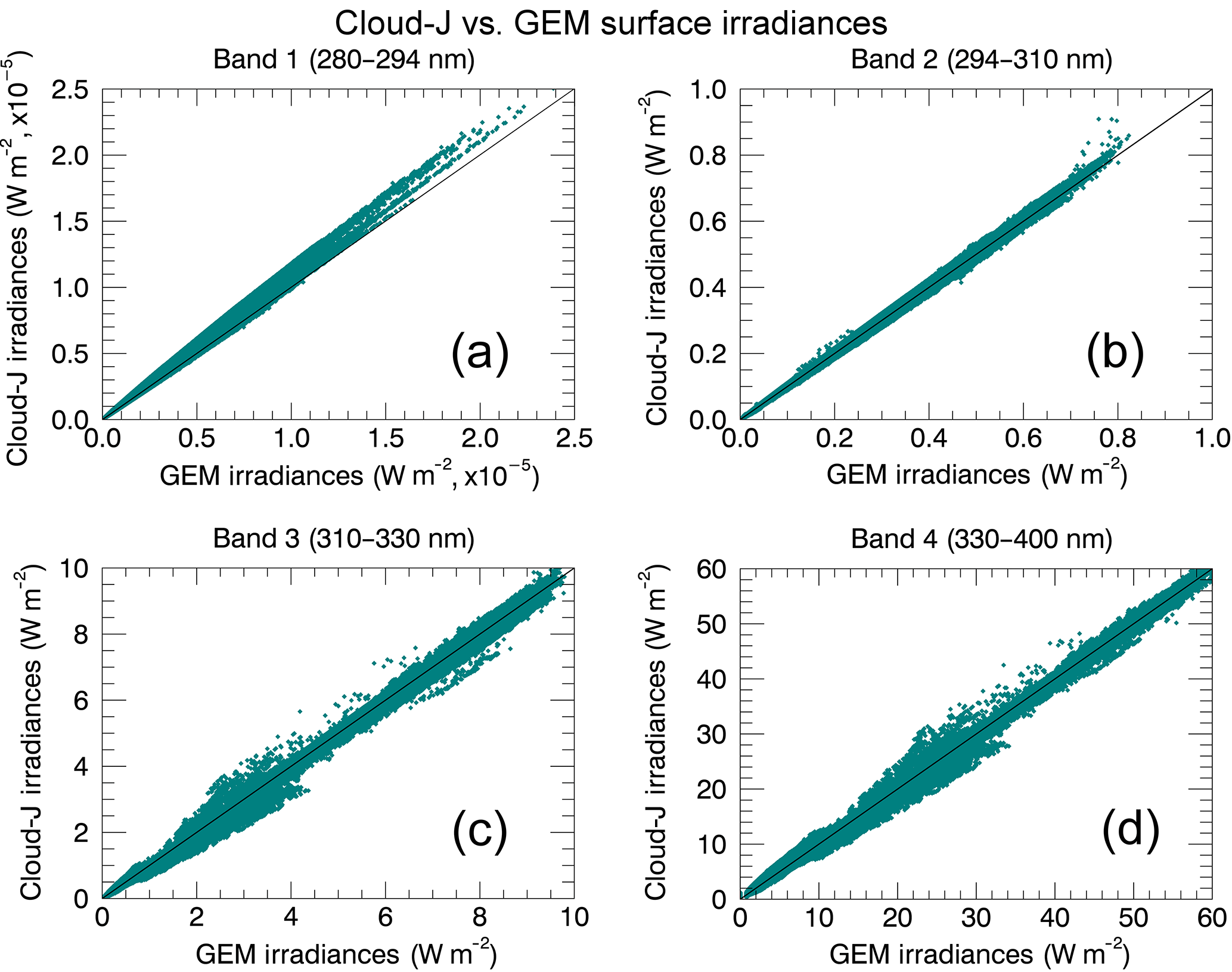
Figure 6 GEM broadband surface irradiances compared to simulated irradiances generated with Cloud-J, where the Cloud-J calculations were performed using the broadband absorption cross section and TOA solar fluxes associated with the correlated-k scheme used by GEM for each UV sub-band. Correlations represent the single-day irradiance contribution for 23 August 2015.

3 Results

3.1 Clear-sky conditions

3.1.1 Broadband irradiances

The comparisons made between GEM and Cloud-J broadband irradiances for clear-sky conditions shows a fairly good agreement in the 311–330 and 330–400 nm bands. For these bands, the linear correlation agreement between the two models is typically greater than 95 % with associated root-mean-square relative errors of 6.4 and 4.0 % for midday values. However, underestimations of GEM irradiances were found in the order of ∼ 30–50 % for the 294–311 nm band and by a factor of ∼ 30 for the 280–294 nm band as shown in Fig. 5b and a, respectively. It was subsequently identified that the bulk of the differences for the two lower bands, especially the disparity in curvatures in bands 1 and 2 in Fig. 5, stems from differences in equivalent broadband absorption cross sections if not also TOA solar fluxes. This is further supported by the significantly improved agreement demonstrated in Fig. 6 where the cross sections of the correlated-k approach cited in Table 6 of Li and Barker (2005) and the solar broadband TOA fluxes employed by the GEM model were instead applied in the Cloud-J calculations. It should be noted that the band solar fluxes used in GEM differ by approximately 0.02 to 0.15 % from the UV sub-band solar fluxes reported in Table 6 of Li and Barker (2005).

A direct comparison was made between the GEM TOA solar fluxes and the broadband averages that were calculated from Cloud-J using the data obtained from Dobber et al. (2008). There are significant differences in the two short-wavelength broadbands with the band values calculated from the Dobber et al. (2008) fluxes being smaller than the GEM fluxes by 35 and 15 % for the 280–294 and 294–311 nm bands, respectively; values for the higher bands are only 3 % smaller and 2 % larger, respectively. These differences would favour an underestimation of the Cloud-J irradiances relative to GEM at the shorter wavelengths in the absence of differences in cross sections, which is opposite to the results in Fig. 5. A comparison to the band averages derived from the solar flux spectrum of Chance and Kurucz (2010) gives smaller differences of −12, 2, −1, and 3.5 % relative to the GEM values.

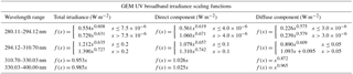
Table 1 Sets of scaling functions to calibrate the GEM UV broadband irradiances to emulate the simulated broadband irradiances produced by Cloud-J. Functions were obtained for total surface irradiances and also their direct and diffuse components.

The spectrally, uniformly weighted average cross sections from the GEISA data set which represent the four UV broadband irradiances are about 24–32 % larger than the values reported in Table 6 of Li and Barker (2005), this also being inconsistent in implication with Fig. 5. However, these estimates do not account for the non-linear impact of the strong spectral variation in absorption cross sections from the GEISA database at lower wavelengths in the UV spectral range shown in Fig. 7. Effective band cross sections from the GEISA spectrum were also calculated for each spectral region for irradiances at the surface using

$$\begin{array}{}\text{(4)}& c_{\text{eff}}={\displaystyle \frac{\mathrm{1}}{N}}\cdot \ln \left[{\displaystyle \frac{\sum F_{\mathit{\lambda }}\mathrm{\Delta }\mathit{\lambda }}{\sum F_{\mathit{\lambda }}{\mathrm{e}}^{-N{c}_{\mathit{\lambda }}}\mathrm{\Delta }\mathit{\lambda }}}\right],\end{array}$$

where F_λ denotes the solar spectral irradiances in W (m² nm⁻¹)⁻¹, c_λ are the absorption coefficients set for a reference temperature and pressure of 223 K and 100 mbar, and the N is a total column ozone of 8.07 × 10¹⁸ molecules cm⁻², equivalent to 300 DU. The numerator is equivalent to deriving broadband average solar fluxes from equally weighting values over all wavelengths as in the previous paragraph. The effective cross section estimates calculated from Cloud-J for the two lowest UV bands (280–294 and 294–311 nm), with values of 1.09 × 10⁻¹⁸ and 2.20 × 10⁻¹⁹ cm² molecule⁻¹, respectively, are now instead smaller by 31 and 19 % relative to the cross sections referred to in Li and Barker (2005), implying larger Cloud-J irradiances; values are larger for the higher wavelength bands by 5 % (311–330 nm) and 18 % (330–400 nm). The impact of these differences is made stronger for the lower bands as their absorption cross sections are larger than for the higher bands by an order of magnitude or more; absorption by ozone in the higher bands is comparatively much weaker. The implied tendency is now in agreement with Fig. 5. This suggests weaker atmospheric attenuation at least from using the GEISA cross-section data set instead of the broadband absorption cross sections associated with the correlated-k approach. Taking the spectrally dependent cross sections and solar fluxes used with Cloud-J as more reliable references, then one or both elements of the broadband cross section and solar flux pairs associated with Li and Barker (2005) and GEM for the lower bands could be considered less optimal for determining irradiances at the surface. This stance is supported by the better agreement, for the six stations in Sect. 2.2, between the Cloud-J and Brewer sample spectra, especially for the dominant 295–310 nm band.

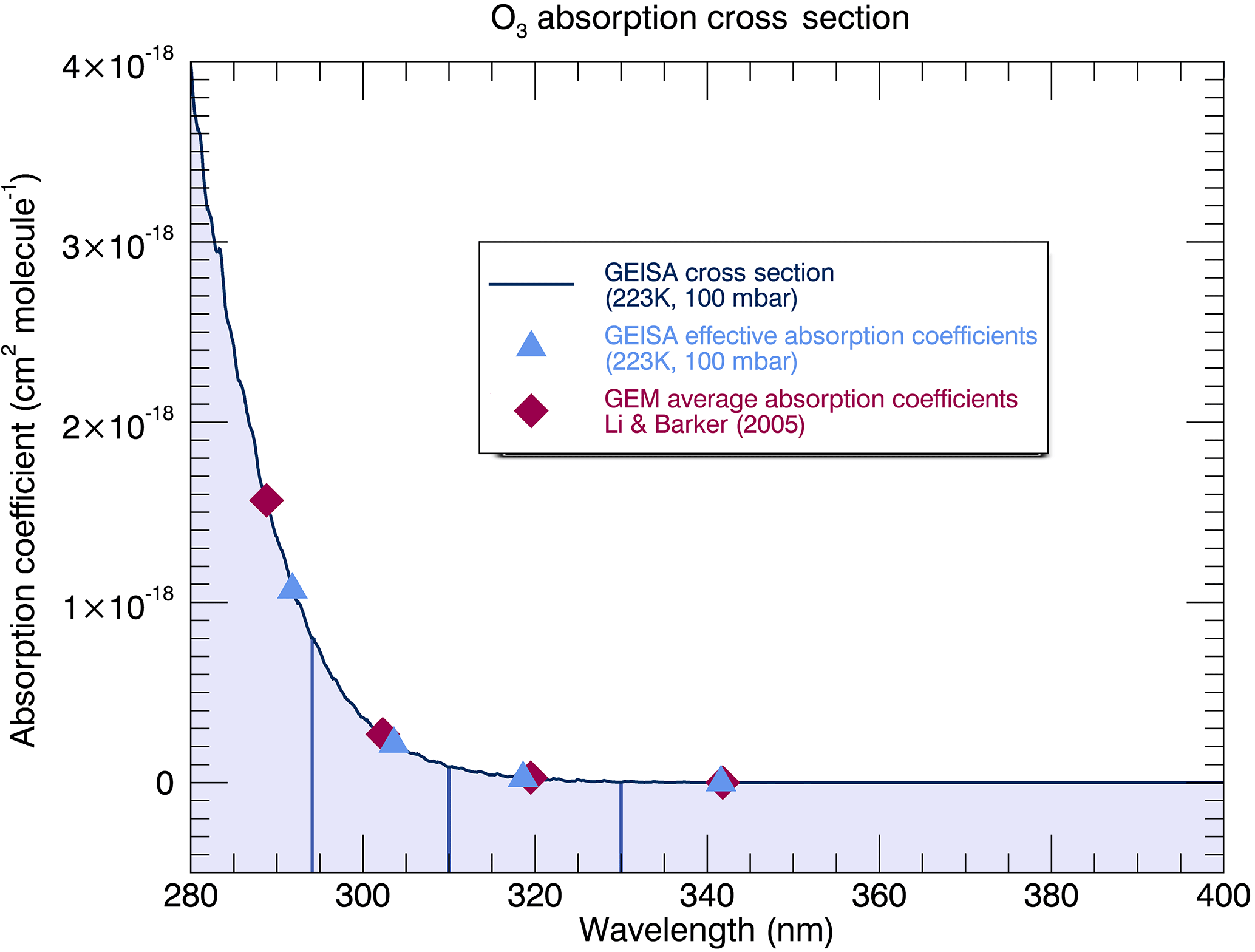
Figure 7 GEISA ozone absorption cross sections measured at a temperature and pressure of 223 K and 100 mbar, respectively. Overlaid are the effective absorption coefficients calculated from the GEISA cross section, as described in Sect. 3.1.1, and the GEM average absorption coefficients for each representative UV broadband region.

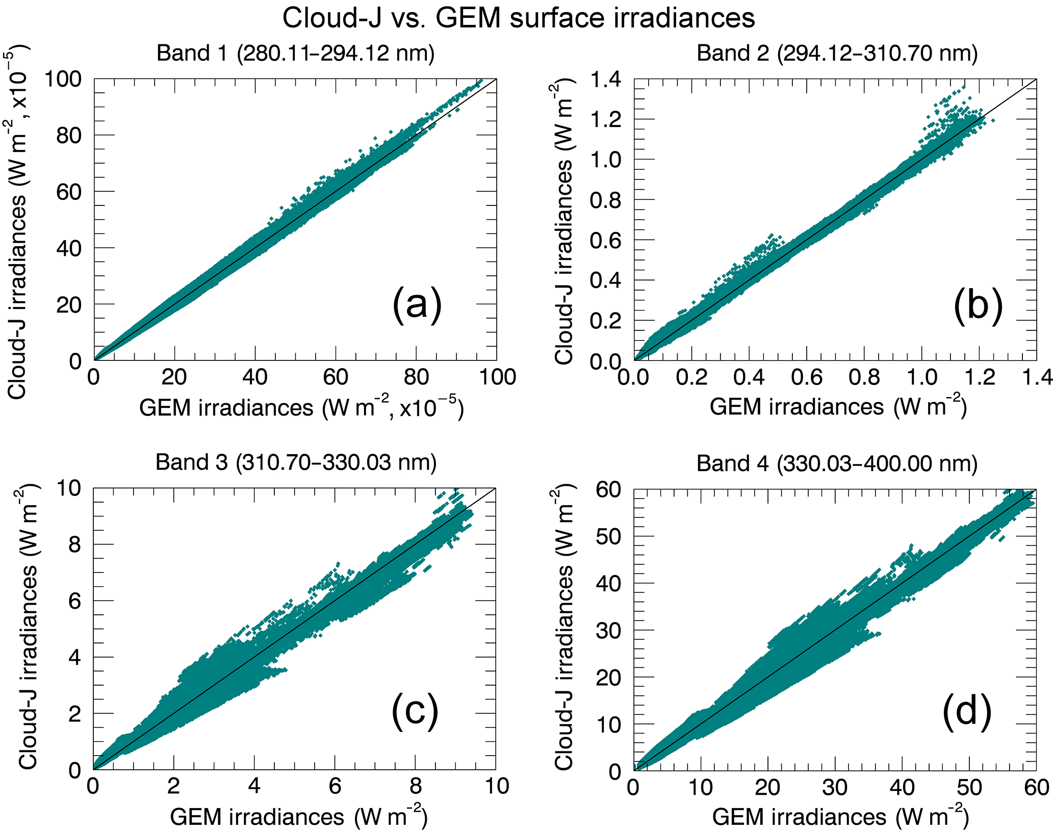
Figure 8 Calibrated GEM broadband irradiances, corrected using the total irradiance scaling functions found in Table 1, compared to the simulated GEM broadband irradiances produced by Cloud-J.

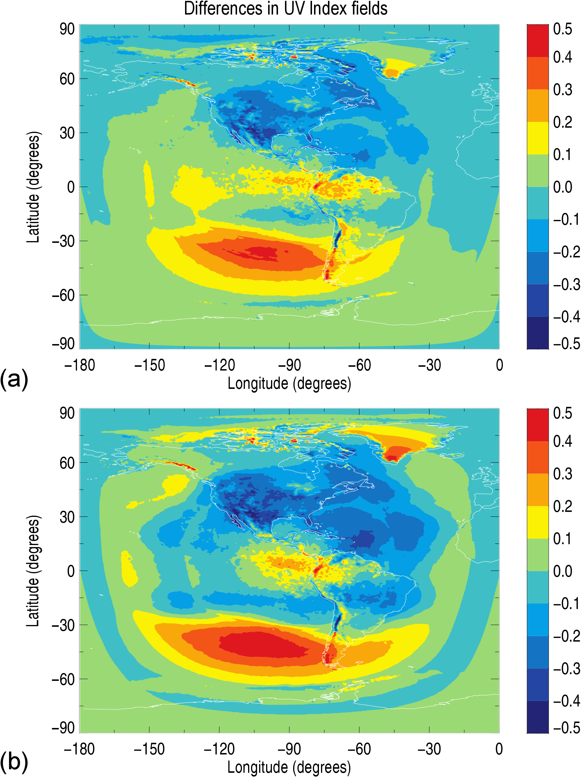
Figure 9 Differences in the UV Index field produced from the scaled and weighted GEM irradiances compared to the field produced using the high-resolution Cloud-J irradiances for the integration approach and linear fit, representing plots (a) and (b), respectively.

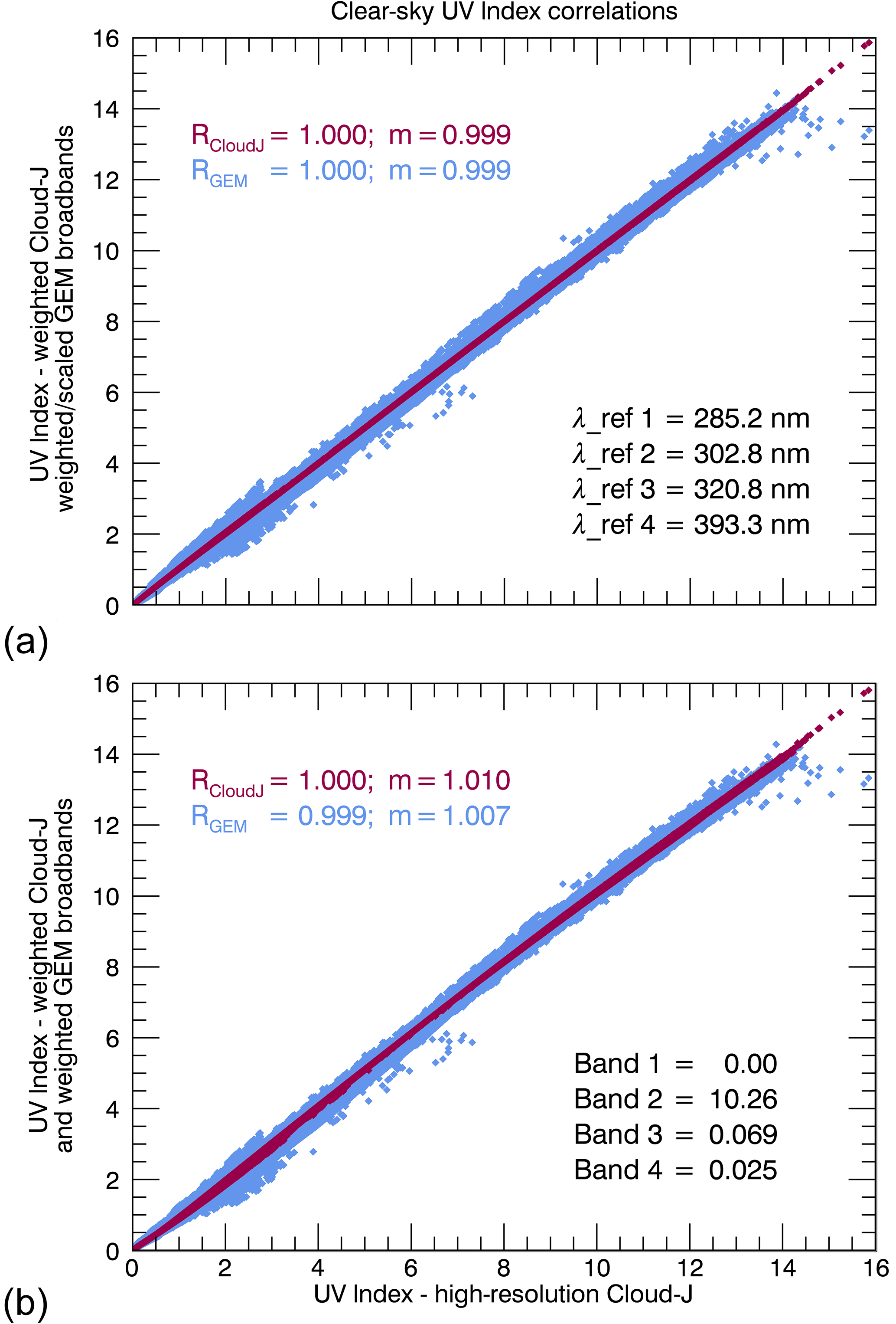
Figure 10 Correlation of the UV Index fields generated from the Cloud-J (purple) and GEM (blue) broadband irradiances. Results from the least-squares minimization using the integration approach (a) produced reference positions of 285.2, 302.8, 320.8, and 393.3, respectively, for each UV sub-band. Minimization performed using the direct linear fitting method (b) produced coefficients of 10.26, 0.069, and 0.025 for bands 2 through 4, respectively, where the weighting for band 1 was intentionally fixed to a value of zero.

Considering the above analysis of the differences in broadband irradiances shown in Fig. 5, scaling of the GEM irradiances to the Cloud-J broadband irradiances was applied as functions of the irradiance values for each spectral band. While contributions to the UV Index from the 280–294 nm band itself could be neglected for total column ozone above roughly 150 DU, scaling functions for this band were still generated since the band value is used in the spectral interpolation to higher wave numbers for the second UV Index model of Sect. 3.1. Also, scaling for the two highest UV bands is not essential and was performed here for completeness. Fits were generated using the 7-day contributions for the total, direct, and diffuse irradiances of the four bands under clear-sky conditions (23–29 August 2015). The scaling functions are provided in Table 1. The correlation of the broadband Cloud-J and the scaled GEM total irradiances obtained for clear-sky conditions are provided in Fig. 8.

3.1.2 UV Index from broadband irradiances

The UV Index fitting based on the Sect. 2.3 integral approach applied to GEM scaled broadband irradiances provided reference positions of 285.2, 302.8, 320.8, and 393.3 nm for bands 1 through 4, respectively, while the straightforward linear fit yielded

$$\begin{array}{}\text{(5)}& \text{UVI}=\mathrm{10.26}{I}_{\mathrm{294}\text{–}\mathrm{311}}+\mathrm{0.069}{I}_{\mathrm{311}\text{–}\mathrm{330}}+\mathrm{0.025}{I}_{\mathrm{330}\text{–}\mathrm{400}},\end{array}$$

where the first coefficient was derived analytically as mentioned in Sect. 2.3. Most of the sensitivity to ozone variability is typically reflected in I_294–311 as absorption from ozone is comparatively weaker for the upper wavelength bands. Reductions in column ozone by 20 % from 300 DU imply changes of about 38, 8.6, and 0.15 % in UV Index from the last three terms, respectively, when the Sun is directly overhead.

Differences of the clear-sky UV Index field between the Cloud-J and resulting GEM values are shown in Fig. 9 and are found to be typically less than 0.2–0.3 for both the integration (panel a) and linear fit (panel b) approaches. The integration approach provides better agreement with Cloud-J, this by up to about 0.1–0.2 for some locations. Over North America, the resultant UV Index values are usually smaller than the Cloud-J-based values by 0.1 to 0.3. Both plots also demonstrate an extended circular region at high zenith angles in the Southern Hemisphere with positive differences reaching up to ∼ 0.5 in the South Pacific area. These larger differences are coincident with UV Index values near the threshold value of 3 used in the least-squares minimization of the scaled GEM broadband irradiances to the high-resolution UV Index field produced by Cloud-J. In addition, there are a sparse number of hot spots which are primarily confined to the Arctic and the high-altitude regions of the Western Cordilleras of North and South America. Here, the differences in the UV Index range between 0.2 and an extreme of 2.4, where the largest differences are confined to a few isolated mountain peaks in Ecuador and the Southern Patagonian Ice Fields bordering Argentina and Chile. The source of the hot spots was determined to be originating from the diffuse component of the calculated surface irradiances, where it was ascertained that the cause was ultimately due to differences in the albedo values used by the GEM and Cloud-J models, where the GEM albedo values underestimate the snow/ice reflectivities in these regions. UV surface reflectivities for snow/ice are typically > 85 % (Chadyšien and Girgždys, 2008) and are readily observed in the OMI monthly average surface reflectivities used by Cloud-J. Although the GEM albedo values for these same regions are also elevated, with respect to the surrounding terrain, they are typically smaller by 35–50 % as compared to the OMI-based climatology.

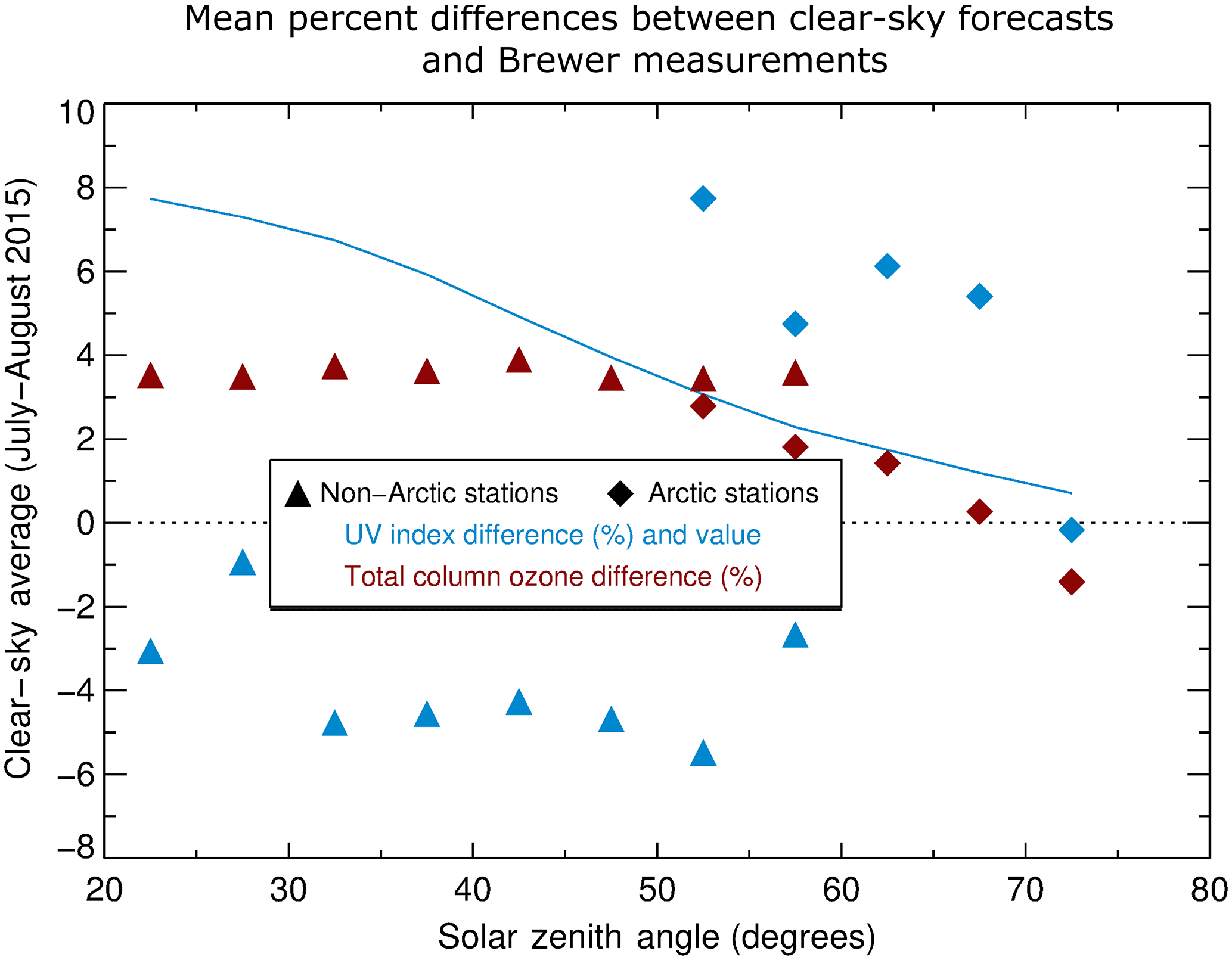
Figure 11 Average UV Index and total column ozone relative differences between the model forecasts and Brewer measurements as a function of solar zenith angle for daytime clear-sky to lightly cloudy conditions for both sets over July and August 2015. This is accompanied by the corresponding average UV Index values. The averages are over 5^∘ intervals in solar zenith angles over the two Arctic stations (Eureka and Resolute) and four non-Arctic stations (Churchill, Edmonton, Saturna, and Toronto) of Fig. 4. The resultant numbers of averaging points per bin range from 30 to 1002 with statistical outliers having been removed in final averages. Model forecasts with output for station locations every 7.5 min were generated from weather and ozone analyses for 00:00 and 12:00 UTC.

Curiously, there is a notable cold spot in the plots of Fig. 9, and it too occurs in South America along a large barren desert tract of the Andes mountains in northwestern Argentina, northern Chile, and southwestern Bolivia. Here, the GEM model indicates that surface reflectivities are elevated to values ranging from 60 to 75 %, much higher than those associated with the snow/ice albedos representing the Southern Patagonian Ice Fields. OMI, however, produces reflectivities of only 10–15 %, making little distinction with the surrounding landscape. Further investigation reveals that this region is variably snow covered during the winter months of the Southern Hemisphere, where the presence of snow is not consistent throughout the month or from year to year. During the 23–29 August 2015 analysis period used in our study, this corresponding region of the Andes was covered under a fresh layer of snow. This observation is corroborated by both snow depth (SD) data obtained from the GEM model and through visual confirmation using imagery data provided by the Moderate-Resolution Imaging Spectroradiometer (MODIS) instruments onboard the Aqua and Terra satellites (https://worldview.earthdata.nasa.gov/). Since the OMI albedo data represent monthly mean reflectivities over a 5-year period (2005–2009), it is unsurprising that a variable presence of snow in this region creates disparities with the long-term averaged values recorded by OMI. The averaging would result in an underestimation in the OMI reflectivities, thus creating the observed cold spot seen in Fig. 9a and b.

Figure 10 shows the resultant direct correlations between clear-sky UV Index values obtained from the high-resolution effective spectra vs. those from the broadband Cloud-J and GEM irradiances for both the integration approach (panel a) and direct linear fit (panel b) for the data corresponding to the 7-day contributions over North America and the Arctic on 23–29 August 2015, at 18:00 UTC. The integration approach, used to weight the scaled GEM broadband irradiances (cyan), shows an excellent agreement with the UV Index calculated using the Cloud-J broadband irradiances (purple) where the slope of the curves, m, and associated Pearson correlation coefficients, R, are at unity. The resultant differences in UV indices from the high-spectral-resolution irradiances and the resultant GEM broadband irradiances are typically within 0.2 with a root-mean-square relative error in the scatter of ∼ 5.6 % for clear-sky conditions. The UV indices calculated using the direct linear combination fitting of the GEM broadband irradiances produce similar results, with a root-mean-square relative error in the scatter of ∼ 7.8 % for UV Index values larger than 3.

3.1.3 Comparison to ground-based UV Index measurements

Section 2.2 provided a comparison of simulated Cloud-J and measured Brewer sample irradiance spectra. The comparison with Brewer measurements is extended here to the clear-sky UV Index and column ozone values from the GEM model 24 h forecast output at 7.5 min intervals over successive 12 h forecasts covering July and August of 2015. Figure 11 shows average differences in total column ozone between the model output and Brewer measurements in the range of 3.5–3.9 % for the four non-Arctic stations with a decrease toward zero at higher latitudes for the two Arctic stations, Eureka and Resolute. This is consistent with column ozone differences stated in Sect. 2.2.

Values for the average UV Index corresponding to their associated column ozone concentrations were generated from the model output using the simplified spectral integration approach. The average UV Index differences between the model forecasts and the Brewer spectrophotometers are −1 to −6 % for the non-Arctic stations, which is partly explained by the differences in column ozone, and 0–8 % for the two Arctic stations.

The change in the sign of the differences for the two Arctic stations might be partly attributed to the relative increases in contribution from irradiances for bands above vs. below 311 nm at higher solar zenith angles combined with the mean irradiance differences with Brewer spectrophotometers above and below 311 nm, mentioned in Sect. 2.2. The cause of the high-latitude disparity in the UV Index observed when comparing between the non-Arctic and Arctic stations in the overlap 50–60^∘ region of Fig. 11 is not known. One possibility may be linked to a geographically varying residual error of the GEM UV Index relative to the Cloud-J value. Still, considering the small UV Index values at high solar zenith angle larger than ∼ 50 degrees, these translate to absolute differences with Brewer spectrophotometers of less than 0.4. The negative differences in UV Index of −1 to −6 % for the non-Arctic stations are usually larger (towards the negative) than the differences of Cloud-J irradiances from Fig. 4. Potential contributing sources of these differences are the residual errors from the fits for irradiances and for the UV Index, the latter having been performed considering only values larger than 3; Fig. 9 indicates roughly −0.1 to −0.3 differences between GEM and Cloud-J over much of Canada. Reducing model ozone biases would improve the agreement with clear-sky Brewer UV Index values by a few percent for UV Index values above ∼ 3–4 or solar zenith angles below 50–60^∘.

3.2 Cloudy-sky conditions

As described in Sect. 1.2, the Cloud-J model possesses a number of options for the treatment of clouds in its radiative transfer calculations. Cloud-J broadband irradiances were produced for each of the cloud options representing cloudy-sky conditions, 2–8, using the GEM parameters for liquid and ice water partial column amounts of each model layer in the presence of clouds and the associated cloud fractions, which are required input for Cloud-J. The simulated broadband irradiances produced by Cloud-J for each cloud option were then compared to the GEM analogs to determine which Cloud-J cloud flag produces output that best reproduces the GEM cloud-sky surface irradiances.

Prior to performing the comparative study, it was recognized that fundamental differences existed between Cloud-J and GEM with respect to the handling of clouds, particularly with respect to the scattering of light with parameters specific to water droplet and ice crystal size. Unlike GEM, the Cloud-J model does not specifically differentiate water droplets and ice crystals into different size bins and determine the scattering contribution accordingly. Instead, for water, an average droplet size is determined for the total water content in a particular model layer depending on the temperature and pressure associated with the model layer. Ice crystals are not differentiated by size at all, only by crystal shape (hexagonal, amorphous), which is also determined by the given temperature and pressure of the model layer. Ultimately, it was determined that Cloud-J cloud option 3 produced cloudy-sky surface irradiances that best emulated the GEM analog. This option was therefore applied for the UV Index comparisons in this section.

The estimation and evaluation of the UV Index estimated under cloudy conditions in this study has been limited to the consideration of two points. One is whether or not the UV Index equations derived from clear-sky conditions are appropriate for cloudy conditions. The other determines the level of impact of radiative transfer differences in the treatment of clouds on differences in derived UV Index values.

The validity of the clear-sky UV Index equations for cloudy conditions was tested using Cloud-J simulations. The clear-sky equations were applied to the Cloud-J broadband irradiances for comparison to the UV Index values derived from the high-resolution Cloud-J spectra for the actual sky conditions from GEM-LINOZ, the latter being a mixture of clear-sky and cloudy-sky conditions. It was found that the equations derived for clear-sky conditions and applied to cloudy conditions with Cloud-J broadband irradiances give essentially the same results as the UV Index values from the high-resolution spectra, i.e., no visible scatter about the diagonal is observed for the corresponding differences in Fig. 12a. Therefore, these equations would also be valid under cloudy conditions and do not require further adjustment.

The remainder of this section examines the impact of differences in cloud radiative transfer. Figure 12a shows the analogous correlations of the UV Index fields generated from the Cloud-J and GEM broadband irradiances under all-sky conditions using the Cloud-J cloud option 3. The weighting was performed using the values obtained though the integration approach of the GEM broadband irradiances under clear skies. Weighting of the all-sky broadband irradiances using the values obtained from the linear fitting approach produce similar results. The overall correlation of the Cloud-J data is in fairly good agreement with the GEM data, but there is an overall increase in error between the two data sets with increasing values of the cloud fraction. To better visualize the distribution density of the correlation, a density plot is also provided in Fig. 12b. We observe that the vast majority of points that fall along or near the regression line, largely, but not entirely, represent those surface irradiances under cloudless or light-cloud conditions. The probability of deviation from the regression line typically increases with increasing cloud cover. This is demonstrated in Fig. 13.

Figure 12 Analogous correlations of the UV Index fields generated from the Cloud-J (purple) and GEM (blue) broadband irradiances under cloudy-sky conditions using Cloud-J cloud flag option 3 in the comparison. Panel (a) presents the direct linear correlations of the UV Index calculated using the GEM and Cloud-J broadband irradiances relative to the high-resolution output produced by Cloud-J using the same scaling functions and weighting determined through the integration approach under clear-sky conditions. Panel (b) is a density plot of the correlation of the UV Index calculated using the GEM broadband irradiances compared to the Cloud-J high-resolution UV Index field depicted in the upper panel.

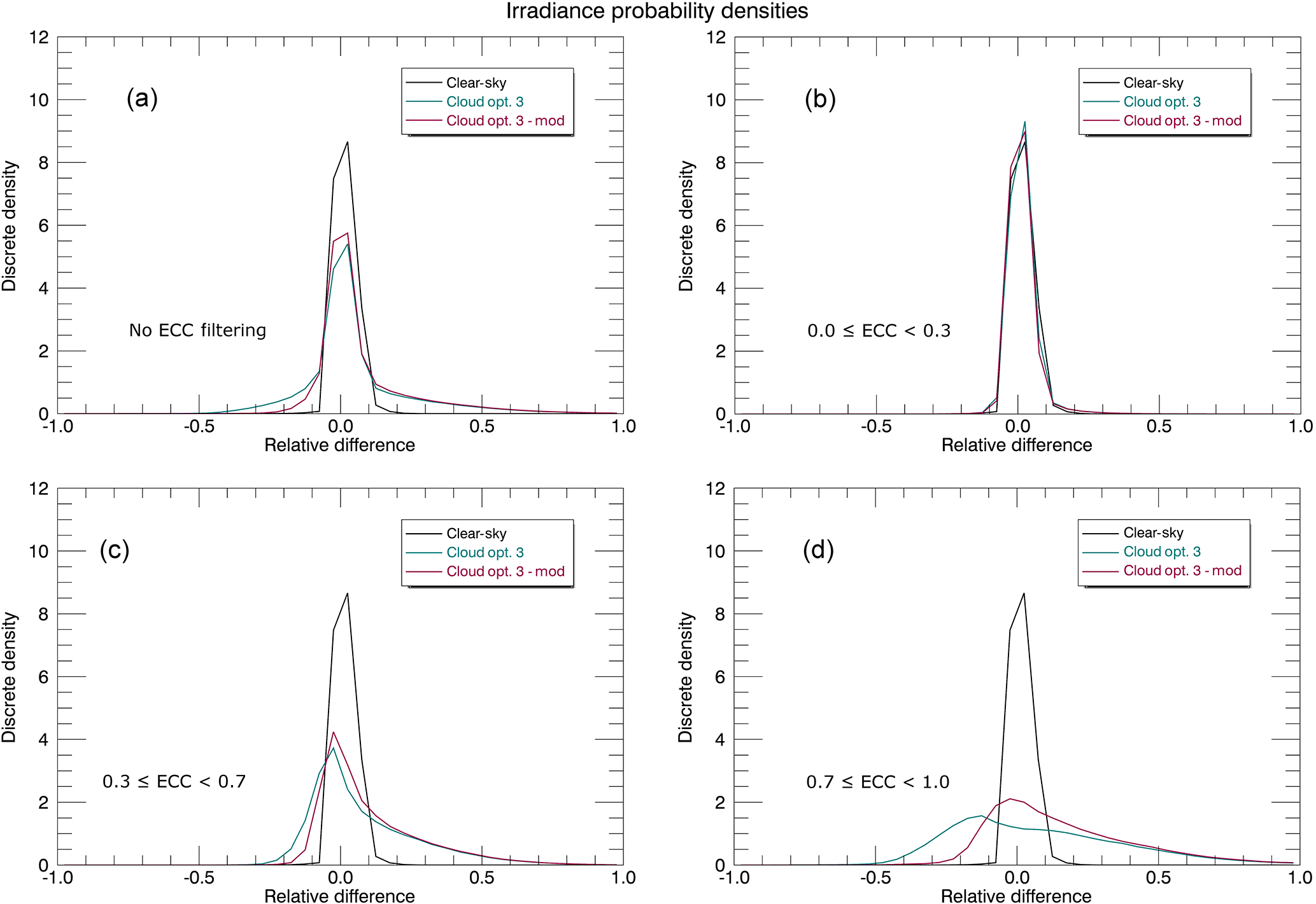
Figure 13 Irradiance probability density plots demonstrating the dependence of the 330–400 nm surface irradiances on effective cloud cover (ECC). Plotted are the relative differences between the Cloud-J and GEM surface irradiances under unattenuated, clear-sky conditions (black), cloudy sky where the Cloud-J option 3 cloud flag is used to calculate cloud attenuation (green), and a modified version of the GEM model output for cloudy skies compared to the Cloud-J data employing the option 3 cloud flag (purple). The modification made to the GEM code was to change the effective radii for the ice clouds to determine if it made any difference relative to the Cloud-J output. In all four plots, a solar zenith angle filter was applied, in which only surface irradiances pertaining to locations where zenith angles < 70^∘ are used. A secondary filter for varying total effective cloud cover is employed in the plots to display the relative difference in irradiances for a given range of cloud cover from clear sky (0.0) to completely overcast (1.0).

Figure 13 contains a series of probability density plots to visualize the dependence of differences in surface irradiances on cloud cover for the 330–400 nm band. Relative differences are observed between the Cloud-J and GEM surface irradiances under unattenuated, clear-sky conditions, as well as for different total effective cloud fraction intervals. To filter for cloud cover, we used the GEM variable for total effective cloud cover (ECC), which reflects the product, the cloud fraction, and opaqueness. ECC is employed in the plots to display the relative differences of the GEM and the Cloud-J irradiance values for a given range of cloud cover from clear sky (0.0) to completely overcast (1.0). Only surface irradiances pertaining to zenith angles < 70^∘ were included to remove larger systematic relative differences at high zenith angles where irradiance values are smaller. The Cloud-J cloud option 3 is used to calculate cloud attenuation in all cases. Output from two different settings of the GEM radiative transfer package for cloudy skies separately provided for Cloud-J simulations and compared to the corresponding GEM irradiances.

Overall, the resultant differences in UV Index values from the high-spectral-resolution irradiances and the GEM broadband irradiances have a distribution for ECC < 0.3 similar to that for clear-sky conditions (Fig. 13b). Under stronger attenuation due to clouds, a substantial increase in the root-mean-square relative error of up to 33 % is observed due to differing cloud radiative transfer models, this involving UV Index values of 1 or larger.

The modification made to the GEM code from its reference settings of Sect. 1.1 was to increase the overall size of the effective radii for the ice clouds from a constant of 15 µm to values in the range of 20–50 µm to determine if it made any difference in relation to the Cloud-J output. As noted earlier in this section, Cloud-J does not differentiate between particle sizes in ice clouds. In the plots, we observe the increase range of relative differences with increasing cloud cover, where differences can reach as high as 100 % and above where the cloud fraction is ≥ 0.7 (Fig. 13d). This implies that different cloud radiative transfer settings (and models) can result in very large differences in UV Index in the presence of optically thick clouds. Also notable is the overall improvement on the left-hand side of the distributions when the ice particle size was increased. This illustrates the sensitivity of irradiances to cloud-related model parameters. To quantify this sensitivity, the percentage contribution of the total discrete densities are compared for the relative differences in the ranges of −0.2 to 0.2 for cases representing 0.3 ≤ ECC < 0.7 (moderate to heavy cloud) and ECC ≥ 0.7 (heavy cloud to completely overcast) conditions, Fig. 13c and d, respectively. Under moderate to heavy cloud cover, the density distributions are similar in nature, where the percent contributions for both the modified and unmodified versions of the GEM model are ∼ 76 %. For heavy cloud to completely overcast skies, there is a marked difference in the percent contributions. The unmodified GEM model cloud scheme produces a distribution in which 50 % of the discrete density is located within the −0.2 to 0.2 range for the absolute relative differences. Using the modified scheme, this value is increased to 62 % stemming from more relative differences of smaller absolute size. These results and percentages provide some general sense of the potential uncertainties of the UV Index values given possible uncertainties in the accuracy of the cloud radiative transfer models.

4 Conclusions

A successful optimization of UV Index determination from broadband irradiances was performed. The Cloud-J v7.4 radiative transfer model was adapted to provide high-spectral-resolution surface irradiances in the UV, 280–400 nm. The high-resolution output from Cloud-J is used to evaluate ECCC's GEM forecast model broadband irradiances under clear-sky conditions and to optimize the determination of the UV Index using these coarse-spectral-resolution irradiance broadbands.

The optimization is achieved by creating simulated broadband irradiances using Cloud-J for direct comparison with the GEM broadband irradiances to generate sets of scaling functions to calibrate the GEM values to the Cloud-J output. The scaled GEM broadband irradiances are weighted accordingly such that the global UV Index field produced using the coarse-resolution broadband irradiances subsequently replicate the high-resolution UV Index field calculated from Cloud-J. Further optimization with the current setup could still be performed, such as excluding outlier differences and focusing over land areas in the fits and further exploring the differences with the Brewer UV irradiance spectra and UV Index values. The comparison with Brewer data for clear-sky conditions suggests potentially remaining systematic UV Index differences up to about 0.3 to 0.5 in magnitude when the surface reflectivities are sufficiently representative.

It was established that equations for the UV Index calculation determined from clear-sky conditions are also applicable to cloudy conditions. However, as is to be expected, the quality of the UV Index values strongly depend on the accuracy of the representation of clouds and, as implied in the limited evaluation of Sect. 3.2, on the accuracy of the cloud radiative transfer model. With formulations as developed here, the improvement of the quality of the UV Index would follow the improvement in accuracy of these factors.

Outlier differences in UV Index values under clear-sky conditions exemplified the relevance of using sufficiently representative surface reflectivities for snow- and ice-covered surfaces. Other factors, such as changes in the applied aerosol climatology or adjustments in the clear-sky irradiance calculation model might potentially warrant a revisiting of the fit coefficients.

The model simulations from Cloud-J, GEM, and similarly from other numerical prediction models pertain only to the consideration of atmospheric columns directly overhead. While the solar zenith angle is reflected in the overhead column attenuation, the atmospheric conditions along the slanted viewing column may differ, thus affecting the actual surface irradiances and UV Index. Moreover, for non-uniform cloud opacity, cloud scattering from various directions is unlikely to be correctly reflected from the overhead column or the solar viewing column alone. Accounting for these aspects, which is beyond the scope of this study, could further improve the accuracy of UV Index forecasts.