the Creative Commons Attribution 4.0 License.
the Creative Commons Attribution 4.0 License.
 | 29 Sep 2022
Atmospherically Relevant Chemistry and Aerosol box model – ARCA box (version 1.2)
Carlton Xavier
Lukas Pichelstorfer
Putian Zhou
Tinja Olenius
Pontus Roldin
Michael Boy
We introduce the Atmospherically Relevant Chemistry and Aerosol box model ARCA box (v.1.2.2). It is a zero-dimensional process model with a focus on atmospheric chemistry and submicron aerosol processes, including cluster formation. A novel feature in the model is its comprehensive graphical user interface, allowing for detailed configuration and documentation of the simulation settings, flexible model input, and output visualization. Additionally, the graphical interface contains tools for module customization and input data acquisition. These properties – customizability, ease of implementation and repeatability – make ARCA an invaluable tool for any atmospheric scientist who needs a view on the complex atmospheric aerosol processes. ARCA is based on previous models (MALTE-BOX, ADiC and ADCHEM), but the code has been fully rewritten and reviewed. The gas-phase chemistry module incorporates the Master Chemical Mechanism (MCMv3.3.1) and Peroxy Radical Autoxidation Mechanism (PRAM) but can use any compatible chemistry scheme. ARCA's aerosol module couples the ACDC (Atmospheric Cluster Dynamics Code) in its particle formation module, and the discrete particle size representation includes the fully stationary and fixed-grid moving average methods. ARCA calculates the gas-particle partitioning of low-volatility organic vapours for any number of compounds included in the chemistry, as well as the Brownian coagulation of the particles. The model has parametrizations for vapour and particle wall losses but accepts user-supplied time- and size-resolved input. ARCA is written in Fortran and Python (user interface and supplementary tools), can be installed on any of the three major operating systems and is licensed under GPLv3.
- Article
(5513 KB) - Full-text XML
- BibTeX
- EndNote


Aerosol and chemical models can be categorized by their dimensionality, in which zero-dimensional models are called box models. However, a box model is generally used as a core module in dimensional models (column, regional or global models), and therefore it makes sense to further describe a model by its complexity and level of details in the chemistry and physics. In this respect, aerosol models can be divided in a sectional or modal approach, in which the first uses discretized size representation and the latter treats the aerosol population as a combination of modes (Zhang et al., 1999). The modal approach is often used in global models due to computational efficiency (e.g. the M7; Vignati et al., 2004), but as the sectional approach can be kept coarse enough, models such as SALSA (Kokkola et al., 2018) have found their place in large-scale use, as well as smog chambers. Here we turn our focus to sectional models with detailed chemistry and aerosol processes, which find their use in smog chamber, flow tube or atmospheric conditions. During the last decades of atmospheric research, several numerical process models for simulating gas- and particle-phase chemistry and dynamics have been developed. Examples from recent years include (but are not limited to) KinSim, used in simulating the chemical evolution of various gas-phase species aimed at studying indoor-air chemistry (Peng and Jimenez, 2019), or MAFOR (Multicomponent Aerosol FORmation model; Karl et al., 2022), also a community aerosol dynamics model which includes multiphase chemistry. Often models are focusing on some particular aspect of aerosol dynamics, such as nanoparticle chemistry and dynamics, e.g. MABNAG, (Yli-Juuti et al., 2013), TOMAS and its extension SOM-TOMAS (e.g. Adams and Seinfeld, 2002; Akherati et al., 2020), particle chemistry and fine structure (e.g. KM-SUB; Shiraiwa et al., 2010), or cloud droplet chemistry and processes (CLEPS; Rose et al., 2018). A review paper by Smith et al. (2021) discusses the current status of the understanding of nanoscale aerosol chemistry and also gives a good overview of the many process models that are used to solve aerosol and atmospheric chemistry and dynamics.
The history of ARCA box starts from the four models used by the authors: MALTE-box (Boy et al., 2006, 2011), ADCHEM (Roldin et al., 2011, 2014), ADiC (Pichelstorfer and Hofmann, 2015) and ACDC (Atmospheric Cluster Dynamics Code; McGrath et al., 2012; Ortega et al., 2012). These models have been used to study ambient phenomena, test and study complex chemical schemes, or test specialized applications such as molecular clustering, chemistry and deposition in lungs (e.g. Olenius et al., 2013; Myllys et al., 2019; Boy et al., 2013; Pichelstorfer and Hofmann, 2015; Xavier et al., 2019; Pichelstorfer et al., 2021). The current work is the amalgamation of these models, with the aim of further development as an open-source community model.
When a scientist without prior experience of a detailed process model wants to apply a detailed aerosol process model, often practical problems arise. Many of the models require substantial modification of source codes and programming experience for them to be applicable for a given case study. Available models are usually tailor-made for a particular problem and might not be written with flexible enough code (for example, parameters are hard-coded) and consequently can be vary laborious to set up. Setting up a model involves detailed configuration, usually requiring in-depth knowledge of the code structure, and contains high risk of misconfiguration. The more the model code needs to be modified, the more the probability of introducing bugs increases. These are some reasons why applying complex numerical models can be unappealing. For most scientists, the simulation itself is not the main focus or motivation of the work, and one would prefer flexible and easily applicable tools, with minimal risk of misconfiguration and with a reasonable amount of time spent in familiarization with the tool. Recently, Python-based solutions have become available, e.g. PyCham (O'Meara et al., 2021) and PyBox (Topping et al., 2018). Yet, it can be said that in terms of usability, the scientific tools are not on par with current-generation software in general. To meet these challenges, we introduce the zero-dimensional Atmospherically Relevant Chemistry and Aerosol box model ARCA box (v.1.2.2). One of the objectives of the development has been in applicability of the model. It is flexible regarding the complexity of the chosen chemistry and aerosol composition, as well as the timescale of the simulation. The backbone of ARCA consists of established theories and standard model implementations, but the model is flexible to customization and further extensions. The source code is written in a way that enables the use of additional or substituting parametrizations for the modelled processes. However, the major advantage of ARCA, setting it apart from other current models in its field, is the graphical user interface (referred from here on as GUI). It makes the model easier to apply, greatly increases reproducibility, reliability and documentation of the simulations, provides tools for visualization of the output, and automatizes many steps in model setup and configuration.
This paper is structured in the following way. Section 2 introduces the scope of the model and explains its structure and main functionality. Section 3 describes the scientific theories behind the modules. Section 4 explains the usage of the model, focusing on the graphical user interface. Section 5 shows verification and standard evaluation of the model's modules. Section 6 summarizes technical details about the system requirements, installation, licensing, code availability and further documentation (the ARCA online manual). Section 7 concludes this paper with plans for future development.
When text is written in MONOTYPE, it refers to a user-definable variable name, which is available from the GUI. The full list of these input variables is shown in Appendix A.
ARCA box is primarily intended to be used for studying processes such as gas-phase chemistry and aerosol processes at atmospherically relevant concentrations (trace gases) and conditions (pressure, temperature, humidity, irradiance). A box model is typically used for simulating smog chambers, indoor spaces or other small containers. Additionally, it can be used to simulate ambient (field) processes, as long ). Using a box model instead of a dimensional model in outdoor simulations is beneficial because computational resources can be put in more detailed chemistry and aerosol processes. ARCA is therefore well suited for studying complex processes and developing and testing new (chemical, aerosol, etc.) schemes before implementing them in a dimensional model. In addition to scientific research, due to its ease of use and configuration, ARCA has also been used in teaching aerosol chemistry and physics.
Given a proper chemistry scheme the model can be used to study the formation of chemical compounds from precursors (or their emissions), calculate effective reactivities (inverse of chemical lifetime) with chosen reactants and simulate the effects of dynamically varying conditions to these processes. The particle formation rate module, containing the Atmospheric Cluster Dynamics Code (ACDC; McGrath et al., 2012; Ortega et al., 2012), simulates the production of new nanoparticles by clustering of molecules – by default from H2SO4–NH3 and H2SO4–dimethylamine (DMA) mixtures, but any chemistry can be included, given compatible input data. Any organic compound in the chemistry scheme, whose pure liquid saturation vapour pressure is known (or estimated), can contribute to particle growth by condensation as calculated by the Analytical Prediction of Condensation (APC) scheme (Jacobson, 2005). Aerosol processes further include coagulation losses and growth by Brownian coagulation and losses by external sinks such as wall losses. Because any of these processes can be switched on or off, quantifying their effects to the total dynamics is straightforward. The GUI allows model initialization and constriction in different ways, either through predefined values from files (such as measurements) or by parametric, time-dependent functions, configured graphically in the GUI. Sensitivity studies, used to assess the effects of uncertainties and variability in the model parameters, are done by changing the parameters within some range. To this end, the GUI has tools to create batches of simulations, in which the nominal time-dependent input parameters for selected variables are varied (either by multiplying or shifting) within user-defined ranges and intervals.
2.1 Main assumptions of the model
Like any box model, ARCA does not consider spatial variation and the related processes, most importantly advection (including convection). When simulating ambient (field) processes, we must therefore assume that the conditions are spatially homogeneous. The transport equation, describing the local change in scalar variable S in terms of its total derivative and advection in wind field V, then becomes
which is an acceptable approximation when , as is the case with fast chemical reactions but not necessarily for slow processes like aerosol growth and coagulation losses. This alone will produce inevitable deviation between modelled (following ) and locally measured (following ) time series.
The particles in the discrete aerosol size distribution are assumed to be spherical, liquid-phase droplets with constant density (ORGANIC_DENSITY). Charges are omitted and all particles are treated as electrically neutral (ion-mediated nucleation is considered in the ACDC module, which calculated the stable cluster formation rate). Liquid-phase organic chemistry in the particles, for example polymerization and the consequential effects this has on the thermodynamics (sometimes called ageing), is not considered in the model. In the present model version particles of all sizes – even above activation diameter – are completely void of water, and the dissolution of inorganic compounds is therefore ignored. Some of these restrictions will be addressed in the near-future updates; see Sect. 7, which also discusses some of the possible implications of the currently missing particle-phase chemistry.
The ACDC nucleation module is more flexible than the aerosol module and – given the proper input – would be capable of simulating also hydrated clusters, but presently neither of the included cluster chemistry systems contain hydrated clusters.
2.2 Structure of the model
The main processes modelled in ARCA box are (in the order of execution) (1) gas-phase chemistry, (2) formation of molecular clusters, (3) reversible vapour wall losses, (4) gas-particle partitioning (condensation and evaporation, using the APC scheme), (5) coagulation of particles and (6) wall loss of particles (Fig. 1). The processes – which can be switched on and off in any combination – are executed in a series in which the next process relies upon values which were calculated in the previous process. Compared to a method where all changes within a time step are solved as one coupled system, this has the advantage that adding more processes (or skipping them) is straightforward as they can simply be added to the main loop as a subroutine or module and solved in any suitable way. On the other hand, the forward integration requires that the time step is kept small enough to justify the linearization of a non-linear system. The default time step (10 s) is usually a good compromise between stability and computational efficiency, but the model also includes a time step optimization algorithm (described in Sect. 2.3).
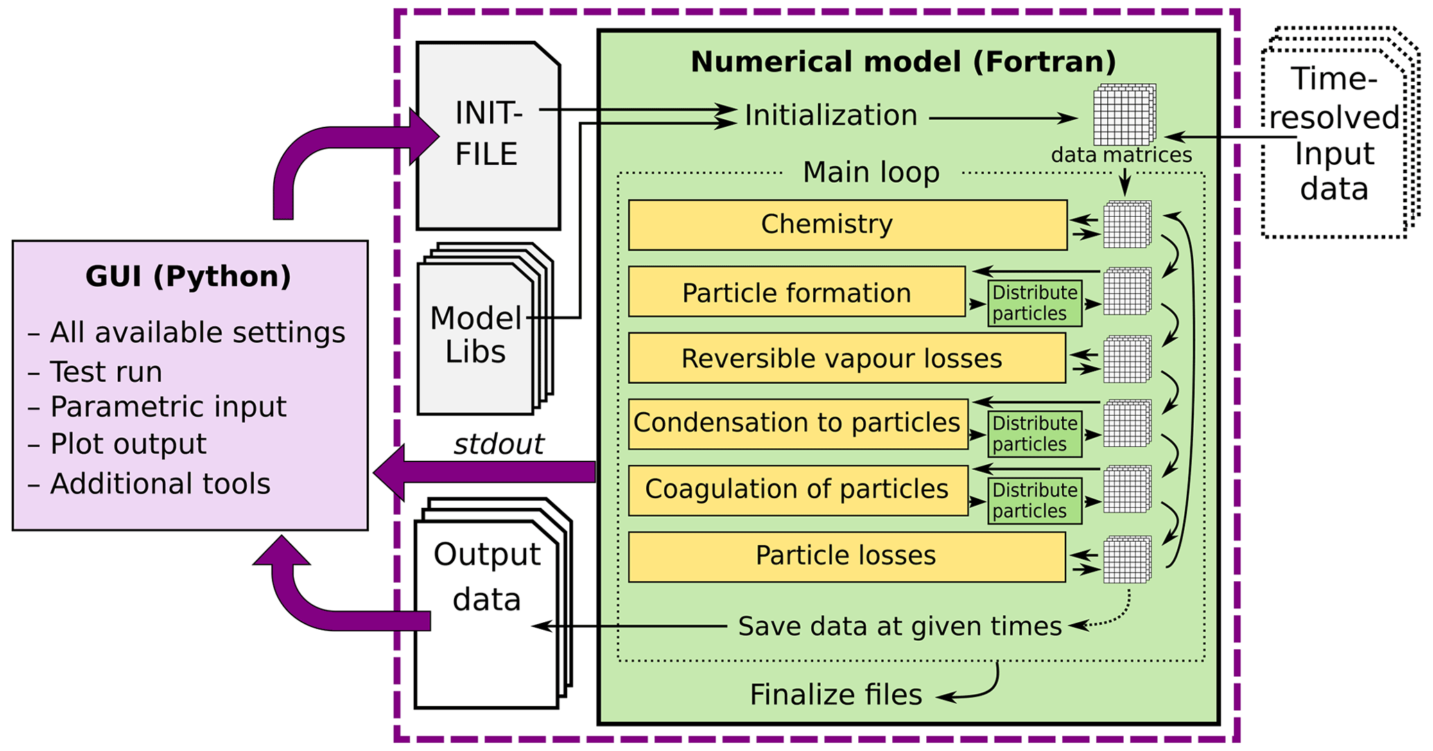
Figure 1Schematic representation of ARCA box. The green rectangle contains the Fortran part of the model, yellow boxes contain the main modules, and the purple box is the Python graphical user interface (GUI). Purple arrows show where the interaction between the GUI and Fortran executable takes place. GUI interacts with the Fortran model by writing the INITFILE (top purple arrow), repeating the screen output of the numerical model (middle purple arrow, stdout) and plotting the output data (bottom purple arrow). The dashed purple rectangle is the minimal configuration needed to run ARCA, and input data are not strictly necessary as parametric input can also be used.
Programmatically the model consists of two main parts: the numerical model (in Fortran), which should be compiled on the computer where it is executed, and the graphical user interface GUI (in Python). Both software environments are freely available for Windows, Mac and Linux, and the model has been successfully installed and used on all three platforms. The numerical module is configured and initialized with a setting file, called hereafter INITFILE, defining all the simulation settings. Additional input includes the spectral irradiance or actinic flux, pure liquid saturation vapour pressures of low-volatility organic compounds and (optionally) the elemental composition of the condensing vapours, and (also optionally) time series of environmental variables, precursor gases, initial or background aerosols, and aerosol loss rates, if the built-in parametrization is not used.
2.3 Model time step optimization
The model can be used with a fixed time step DT (default time step is 10 s) or with multiple, dynamically changing time steps. With the latter the user defines the maximum and minimum relative change in one time step for (1) particle diameter (ddp), (2) particle number concentration in each bin (dNp) and (3) concentration of condensable vapours (dC). After exiting each module (shown in Fig. 1), the changes in 1–3 are calculated. If the module produced changes that exceed the maximum, the time step for that module is halved, and the current integration time step will start over. In contrast, when the largest change is below the tolerance minimum, the time step of that module is doubled. The modules are assigned with one of the three time steps, denoted CCH (condensation and chemistry), COA (coagulation) and DEP (losses). The processes used to control the time steps are shown in Table 1.
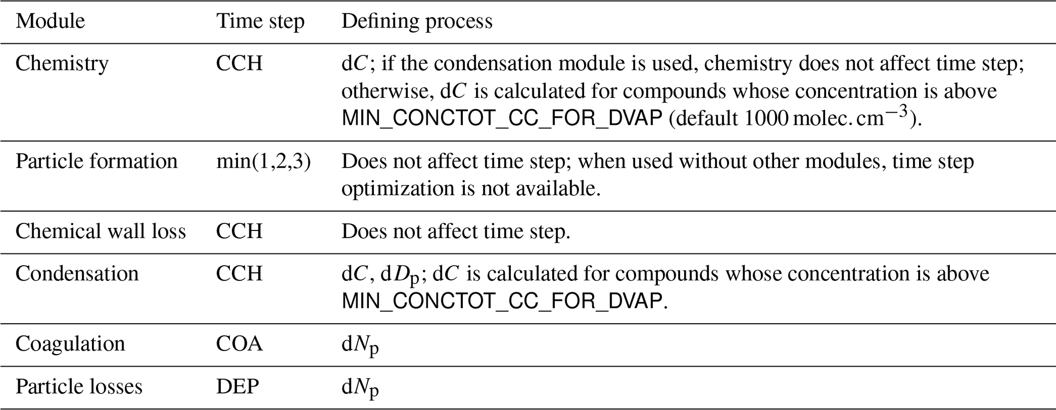
When time step optimization is used, a three-element vector DT_UPPER_LIMIT defines the maxima for CCH, COA and DEP, and the nominal model time is used as a minimum (by default the GUI sets DT to 1 ms). Therefore, the three time steps are defined by multiplying the nominal model time step by a factor of 2n, where , and satisfy . Optimizing time step in this way has two effects. It helps to overcome the potential error created by decoupling of different modules that are not solved together as one dynamic equation (notably condensation to particles and chemistry) by guaranteeing that the changes in one time step are small. On the other hand, when a process is very slow, such as aerosol coagulation, the extra precision gained by a small time step is negligible; instead increasing the time step can shorten the computational time significantly. The effect on the execution time of the simulation depends on the tolerances and the conditions of the simulation. With loose tolerances (5 %–10 %) the simulation time is usually shortened, while tight tolerances (0.2 %–3 %) will increase runtime markedly. The time step optimization should first and foremost be seen as a safeguard against diverging too far from the true solution of the integration.
3.1 The chemistry module
The chemistry code of ARCA is based on the KPP (Kinetic PreProcessor, https://people.cs.vt.edu/asandu/Software/Kpp, last access: 23 September 2022; Damian et al., 2002; Sandu et al., 2003; Daescu et al., 2003), and any reaction set which complies with the KPP format can be used to create ARCA's chemistry modules. An often used source for atmospheric chemistry schemes is the MCM v3.3.1 (Master Chemical Mechanism version 3.3.1, http://mcm.york.ac.uk/MCMv3.3.1, last access: 23 September 2022) (Jenkin et al., 1997, 2015; Saunders et al., 2003), which provides the gas-phase chemical reactions and rates of the degradation of specific organic compounds in the atmosphere, as well as detailed inorganic chemistry and photochemistry. The full scheme – or a subset – can be downloaded from MCM website in KPP format. Optionally, the user might have additional chemistry schemes, which need to be combined with the MCM scheme, such as the PRAM scheme (Peroxy Radical Autoxidation Mechanism; Roldin et al., 2019) which describes the production of highly oxygenated molecules (HOMs) from monoterpenes and is included in the ARCA distribution. ARCA's GUI has a tool (“create chemistry scheme”) which combines different schemes, removes duplicate compounds, and reactions and creates a valid single KPP definition file, used for producing a Fortran module with KPP. A modified source code of KPP v2.2.3, accommodated for very large schemes, is provided with ARCA. The generated code will then be part of ARCA and is available for use after compilation. Switching between different chemistry schemes can later be done in the GUI with a drop-down menu.
3.1.1 Photochemistry
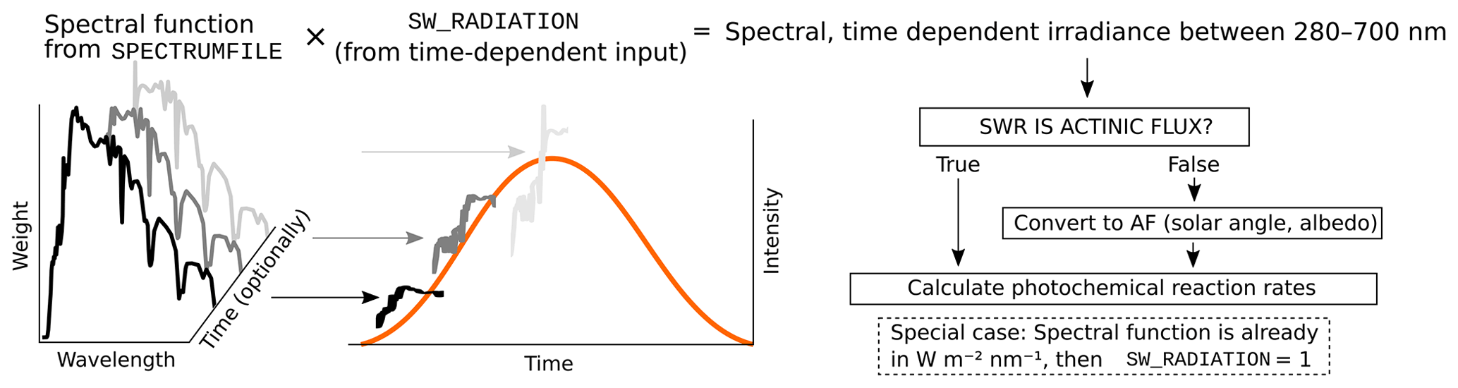
The photolysis rates of the photochemical reactions are calculated by integrating the absorption cross section, quantum yield (provided by MCM v3.3.1) and actinic flux (AF). Actinic flux spectral data (in ) can be sent directly in, or it can be estimated from the global short-wave radiation (in ), surface albedo, geographic location and the date of the simulation, as described in Kylling et al. (2003). The actinic flux and short-wave radiation are wavelength dependent, but often only the total irradiance over a wavelength range is measured instead of the spectral distribution. ARCA contains a generic clear sky spectrum (glob_swr_distr.txt) between 280 nm and 4.8 µm, obtained from the Bird Simple Spectral Model (Bird and Riordan, 1986). There is also a site-specific spectrum for SMEAR II (Station for Measuring Forest Ecosystem–Atmosphere Relations) station in Hyytiälä, Finland, based on measured and averaged yearly spectra from 2001 (Boy and Kulmala, 2002). The spectrum in glob_swr_distr.txt is normalized for the 300 nm–4 µm wavelength range, assuming a flat response from the instrument. Should the actual measurement range differ from this, the user can provide the lower and upper limits of the wavelengths, and the default spectrum will be normalized to this range.
The provided two spectra are somewhat generic and represent field conditions. For more precision – or, for example, smog chamber simulations – the user should provide their own spectral data which must be in 5 nm steps and contain entries from 280 to 700 nm. Exceeding entries in the data file are ignored as they are not relevant in the photochemistry. Spectral data can be a single, constant spectrum or time-resolved. If time-dependent data are provided, a linear interpolation in time is performed at each model time step. The exact format of the spectral file is described in the online manual.
The user-supplied spectral data can be thought of either as a weighing function, whose integral over the measured wavelength range amounts to 1, or as absolute values [ ]. In the first case the time-dependent scalar variable SW_RADIATION represents the measured total irradiance, and in the latter SW_RADIATION is set to a constant (1, or some dimensional factor). Finally, if the option SWR_IS_ACTINICFLUX is selected, the SW_RADIATION and the provided spectral data are directly used as actinic flux []. A schematic representation of the short-wave radiation data processing is shown in Fig. 2.
3.1.2 Reaction kinetics
At each time step, the reaction rates (including photolysis) are updated using current pressure, humidity, irradiation and temperature. With these the chemistry module solves the new concentrations after one model time step. The concentration C of any compound q is described by an ordinary differential equation (ODE).
where Rx,q are the reactions x that either produce or consume the compound q. The ODEs of the compounds in the chemistry scheme form a system of coupled non-linear equations, which is solved numerically in ARCA's chemistry scheme, by default using KPP's general Rosenbrock solver (Sandu et al., 1997).
In ARCA the concentration of any compound in the chemistry can be set to a user-defined value. Typically, this is done for the precursor gases, whose concentrations could be measured or otherwise known. The user-supplied concentrations are read from the input, interpolated to model time and saved in the model data matrix, overwriting previous values. Then, if a compound was defined as fixed in the chemistry scheme (DEFFIX in KPP definition file), its time derivative (Eq. 2) is zero, and the concentrations do not change during the chemistry step; if the compound was not fixed (DEFVAR in KPP definition), the concentrations will in general change (and this would be reflected in the concentrations of its reaction products), but as previously, the resulting concentration will be overwritten in the next time step when the model concentration is set to the given input concentration. The user can also define a time after which the updating of the concentrations of the chemical compounds (and separately for emissions) is stopped, and the chemistry is allowed to “float”, meaning that also the precursor concentrations evolve dynamically without outside interference (if they are DEFVAR). The definition of fixed and varying compounds can easily be done in ARCA's “create chemistry scheme” tool when creating a new chemistry scheme. As a rule, precursors should be defined as fixed unless the simulation involves floating the chemistry, as described above. Figure 3 further explains the effect of these settings on the simulation.
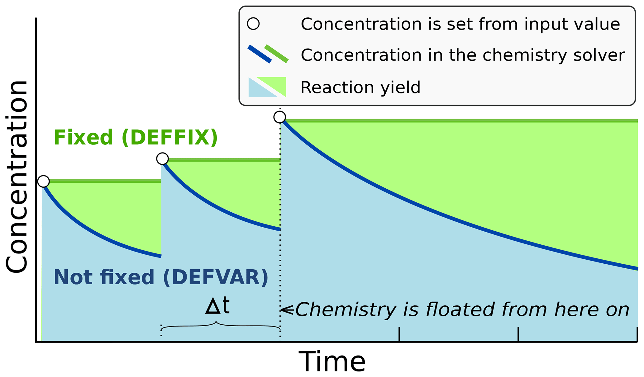
Figure 3Schematic example of the effect of defining a compound in DEFFIX or DEFVAR. In this example, the variable is set by the user (in the GUI, this is done in the tab “time-dependent input”). The solid lines show the concentrations inside the chemistry solver for a compound which is fixed (green curve) and not fixed (blue curve). The circular symbols show the set concentration in each time step. The shaded areas represent the proportional impact of DEFFIX and DEFVAR on the concentrations of the reaction products of the compound. Depending on the model time step Δt, the differences can be substantial and illustrate why the precursors should be set fixed unless the chemistry needs to be floated.
After the chemistry step, all negative values are set to zero. Negative concentrations are non-physical but could emerge from numerical inaccuracies, so a warning is issued if some concentration is less than −100 , as this would be an indication of misconfiguration, such as incorrect units in the input.
3.2 Particle size distribution (PSD)
The main use of ARCA, besides simulating chemical reactions in the gas phase, is to compute the evolution of a population of aerosol particles experiencing dynamical processes such as coagulation, deposition and phase transition. There are many ways to formally approach this task, discussed, for example, by Whitby and McMurry (1997). In the atmosphere, the number of condensing species, different particle sizes and compositions is unlimited, and the practical mathematical descriptions of the PSD therefore require simplifying assumptions. The aerosol dynamics models are often characterized by their representation of the PSD. Typical representation types are the discrete, the spline, the sectional, the modal and the monodisperse representation.
In the discrete representation, particles have a discrete size and composition. That is, one size section includes exactly one discrete particle composition, given by the exact numbers of molecules of different compounds in the particle. This approach must be used when explicitly modelling initial cluster formation but gets increasingly complex and numerically heavy when more “building blocks” are added, such as chemical compounds or particle sizes. ARCA's nucleation module consists of the ACDC model which uses discrete representation.
Sectional models decrease complexity of the system by grouping parameters, and typically the particle diameter range (and equivalently volume, mass and surface) is divided into a limited number of intervals or size bins. Particles in each bin have the same properties. This is a common approach in atmospheric modelling; however, its accuracy depends on the number of bins used and on the magnitude of change applied within one integration time step Δt. While large changes within Δt lead to a deviation from the analytical solution, small changes cause numerical diffusion especially when simulating condensational growth (Gelbard and Seinfeld, 1980).
ARCA allows to choose between two sectional representations, the fully stationary (FS; Gelbard and Seinfeld, 1980) method and the fixed-grid moving average method (MA, also called “moving centre sectional”; Jacobson, 1997a). The future roadmap includes a hybrid method, discussed in Sect. 7. The current representation methods are graphically summarized in Fig. 4.
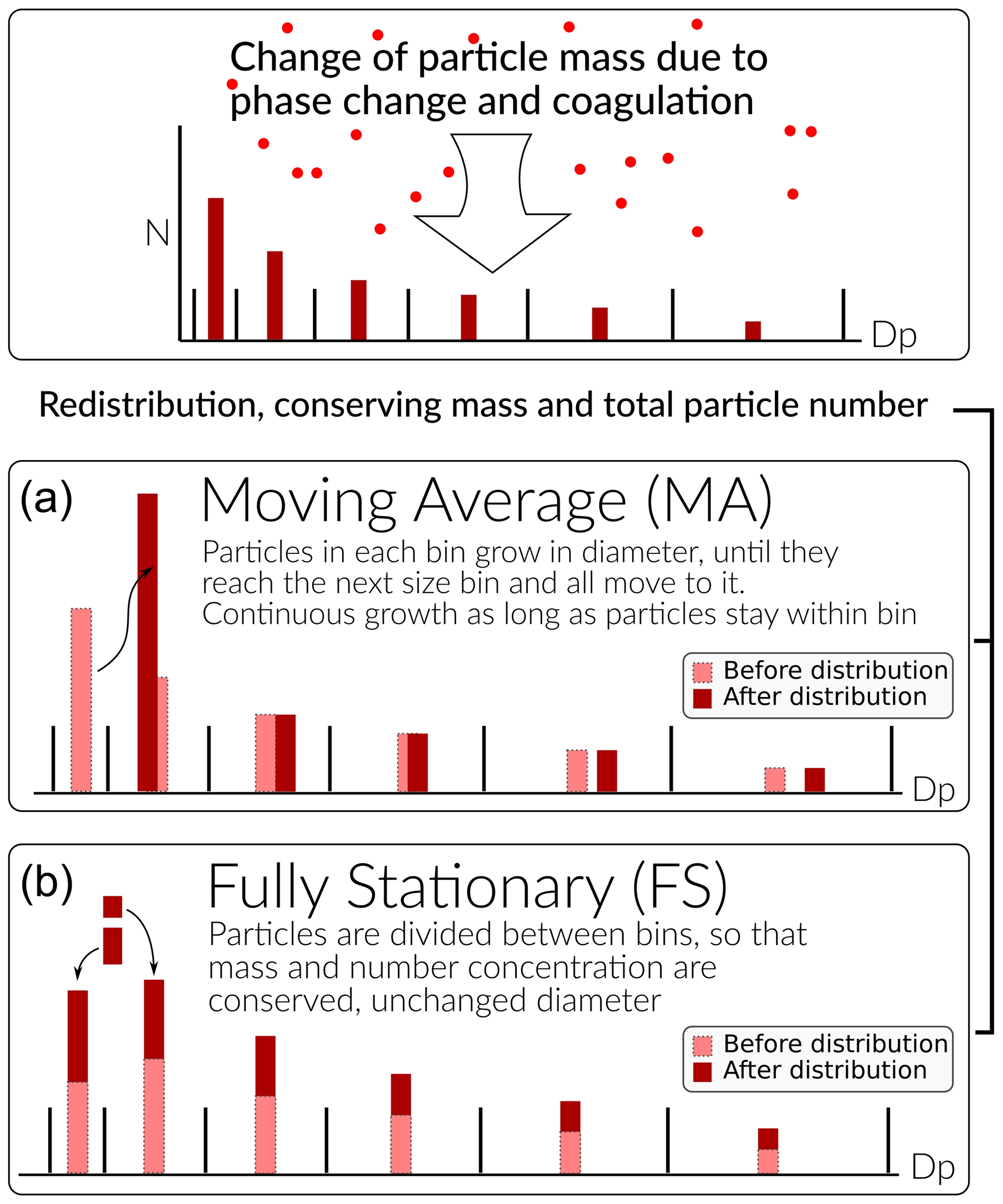
Figure 4Schematic of the two particle size distribution representations: the fixed-grid moving average (MA, a) and the fully stationary (FS, b).
The FS method is very robust during computation but does not treat growth continuously, and therefore it suffers from numerical diffusion (Jacobson, 1997a). This is the result of the redistribution, in which particles are assigned to bins below and above the actual size the particles have grown (or shrank) to be, thereby introducing particles that are larger (or smaller) than those the condensation or evaporation produces. In time this will lead to spreading of the size distribution, much like a diffusive process. The MA method strongly reduces numerical diffusion as the particle diameter within the size grid can continuously change, and particles are not distributed between bins. The main drawback of the MA method is the appearance of numerical artefacts, referred to as “pits” and “peaks”, affecting the analysis of the results. However, they can be removed during data analysis by remapping the data on a new size grid as described by Mohs and Bowman (2011). Both PSD methods used conserve mass and total particle number.
The choice of the PSD representation does not affect the calculations in the aerosol dynamics module as they are separated from each other. This means that the different methods to represent PSDs can be changed or added without interfering with the aerosol dynamics code. Aerosol-related parameters required to solve the dynamics are provided by accessor functions (getters) and work for any PSD representation. Further, changes to the PSD by the dynamic processes are calculated in the aerosol dynamics module but applied in the PSD module. This allows further development of the scientific and computational aspects independently.
3.3 Initial new particle formation by molecular clustering
Formation of new particles from vapours by clustering of gas-phase molecules, often referred to as aerosol nucleation, is described by simulation of molecular cluster population dynamics with quantum chemistry input for cluster evaporation rates. This yields the formation rate of new particles per unit volume and unit time.
3.3.1 Molecular cluster dynamics simulation
Molecular cluster formation dynamics is solved by the ACDC code (https://github.com/tolenius/ACDC, last access: 23 September 2022), which calculates the time-dependent cluster number concentrations for a given set of molecular clusters and ambient conditions. A detailed description of ACDC can be found in Olenius et al. (2013). Briefly, ACDC generates and solves the discrete, molecular-resolution general dynamic equation, also known as the cluster birth–death equation, considering all possible collisions and evaporations among the clusters and vapour molecules, ionization and recombination processes, and external cluster sinks. When a collision results in a cluster that is outside the simulated system, and its composition satisfies the defined stability criteria, it is considered stable enough to not re-evaporate (Olenius et al., 2013). These outgrown clusters constitute the formation rate of new particles.
By default, collision rate constants are calculated as hard-sphere collision rates for collisions between electrically neutral species, as well as according to dipole-moment and polarizability-dependent parametrizations for collisions between neutral and ionic species (by default from Su and Chesnavich, 1982). Evaporation rate constants are obtained from quantum chemical cluster formation free energies. Ionization and the recombination of clusters and molecules occur by collisions with primary ionic species, which originate from galactic cosmic rays and radon decay and are assumed to have the properties of and H3O+. Cluster scavenging sink is obtained from the particle population modelled by ARCA, with sink rates Rsink calculated according to , where Dcluster is cluster diameter, and CSvapor and Dvapor are the condensation sink and diameter of the monomer (H2SO4 is used as proxy), respectively (Lehtinen et al., 2007). CSvapor can also be given as time-dependent input (CONDENS_SINK) if the aerosol module is not in use. The user familiar with ACDC may also modify the rate constants and the settings for the inclusion of different cluster dynamics processes. In addition to the ARCA user manual, the interested reader is referred to the ACDC manual, available from the repository, and references therein.
3.3.2 Available cluster chemistries
The default ARCA has slots for five ACDC modules, which can be switched on and off individually. The current default implementation includes two separate clustering chemistries: H2SO4–NH3 and H2SO4–DMA (dimethylamine), including electrically neutral and negatively and positively charged clusters. Cluster evaporation rates are in the default installation calculated from previously published quantum chemical data computed with the B3LYP/CBSB7//RICC2/aug-cc-pV(T+d)Z level of theory (Olenius et al., 2013), but the user may switch to alternative systems, calculated with DLPNO-CCSD(T)/aug-cc-pVTZ//ωB97X-D/6-31++G** level of theory. The main reasons for applying the B3LYP//RICC2 data are that these cover large sets of cluster compositions including all charging states and perform reasonably well compared to laboratory experiments (Almeida et al., 2013; Kürten et al., 2016). However, cluster evaporation tends to be underpredicted, and thus the formation rates can be considered upper-limit estimates. ARCA's procedures allow easy rebuilding of additional cluster chemistries if the user wants to apply new or updated data for the evaporation rates. Furthermore, the number of slots for ACDC modules can be increased from five with minor code modifications.
3.3.3 Coupling of cluster and aerosol dynamics
The cluster dynamics simulation is implemented by passing the input for the ambient conditions to the cluster formation routine at each model time step. The input includes concentrations of the clustering vapours, temperature, primary ion production rate (if supplied by the user) and condensation sink of H2SO4 (from previous time step or CONDENS_SINK), used as reference molecular size for scavenging sink CSvapor. The cluster formation routine solves the time evolution of the cluster concentrations for the given time step, using the concentrations from the end of the previous time step as initial values, and returns the number of new particles that grow out of the cluster regime during the time step. This is converted to new particle formation rate (by ) and handed to the main module. The newly formed particles are then distributed within the first model PSD size bins in the diameter range of [], with weights calculated by
where d is the index of the bin closest to diameter . This somewhat arbitrary distribution is based on the assumption that some stable clusters result from collisions that would produce larger than the minimum stable cluster and assigns about 75 %–85 % of the newly formed particles to the first bin. The factor to calculate the upper diameter for the distribution (by default 1.15) can be changed with NPF_DIST (e.g. set to 1). The user is responsible for selecting a suitable PSD size range so that the minimum size for the simulation closely matches the size of the outgrowing particles from the ACDC systems. In the case the selected min(dp) in the model is larger than the outgrowing cluster from any of the ACDC subsystems, the model issues a fatal warning in the beginning of the run and terminates. If the outgrowing clusters are more than 10 % larger than min(dp), a (non-fatal) warning is issued in the first time step. The newly formed particles are assigned a general non-evaporating particle composition (in the model called GENERAL).
ACDC has an option to calculate a steady-state formation rate, which corresponds to a time-independent situation in which the cluster concentrations have relaxed to a steady state for the given ambient conditions. The steady-state option (ACDC_SOLVE_SS) must not be used for a dynamic atmospheric case in which the conditions vary with time, and thus the formation rate depends on the immediate history of the conditions. Instead, the steady-state option is useful if the user wishes to run the cluster routine as a stand-alone model and study the dependence of the steady-state formation rate on, for example, vapour concentration or temperature. In general, while the steady-state approximation is necessary for computationally heavier large-scale models, it may cause artefacts especially at low vapour concentrations or dynamic conditions. As an explicit cluster simulation is easily embedded in a box model such as ARCA, it is reasonable to not introduce such an unnecessary potential error source.
3.4 Other options for new particle formation rate
In addition to the explicit cluster dynamics simulation, simplified formation rate parametrization can be used. Currently, a parametrization for new particle formation from H2SO4 and representative organic components is available. This option approximates the formation rate as a function of H2SO4 and user-defined set of organic compound concentrations. The choice of what organic compounds (or proxies for them) to include in the set is not unambiguous and is dependent on the active chemistry scheme and assumptions made by the user. Still, such parametrizations are commonly used to characterize empirical observations of particle formation (e.g. Paasonen et al., 2010). While they do not correspond to an explicit time-dependent formation rate and may not include all independent ambient parameters which could affect the formation rate, they are useful for assessing the magnitude of particle formation through the given chemistry.
To complement the formation rates and the parametrization, the model has also a time-dependent input variable NUC_RATE_IN. When multiple particle formation rates are calculated, either by different ACDC systems, additional parametrizations or NUC_RATE_IN, the total formation rate – used in the aerosol module – is the sum of all processes. The output files contain the total formation rate and separately those from the ACDC systems. Furthermore, if applicable, the formation rates of electrically neutral and positively and negatively charged particles are also saved. It must be emphasized that the charging states refer solely to the charges of the outgrowing particles in ACDC, not to the formation mechanisms of the particles. For instance, newly formed neutral particles may originate – and often do originate (Olenius et al., 2013) – from ion-mediated processes, in which small ions recombine, and the product grows further as a neutral cluster.
3.5 Condensation and evaporation of organic vapours and sulfuric acid
Formation and evolution of either natural or anthropogenic aerosols are dependent on gas-to-particle-phase transition via nucleation, condensation and evaporation (Tsang and Brock, 1982; Wagner, 1982) and further on coagulation (von Smoluchowski, 1918; Fuchs, 1964). In ARCA, the condensational growth of particles due to organic vapours and sulfuric acid is defined by their gas- and particle-phase concentrations and pure liquid saturation vapour pressures psat (sulfuric acid is treated as non-evaporating vapour with psat=0). ARCA employs the mass-conserving Analytical Predictor of Condensation (APC) scheme (Jacobson, 1997a, 2002), describing the condensational transfer of a gas-phase compound q onto particles in size bin i, as the change in particle-phase composition cq,i, in a time interval Δt:
where Cq,t is the gas-phase concentration of compound q at time t, is the equilibrium saturation ratio of the condensing gas, is the pure compound saturation vapour concentration over a flat surface, and is the mass transfer rate between the gas phase and all particles of size i (Jacobson, 1997a). The mass transfer rate [s−1], where ni is the number concentration of particles in size bin i, di is the diameter of the particle in size bin i, and is the diffusion coefficient of compound q with particles in bin i (Jacobson, 1997b). The equilibrium saturation ratio is calculated using the Köhler equation, which combines both the Kelvin and solute effect. The Kelvin effect accounts for the changes in saturation vapour pressure over the particle due to surface curvature, with small particles having larger saturation vapour pressures. The solute effect, or Raoult's law, describes the change in saturation vapour pressures for an ideal solution with a mixture of compounds in the particle droplet. Overall, the equilibrium saturation ratio for a compound is obtained by multiplying the solute effect, expressed as the molar fraction of the compound and the Kelvin term:
where xq,i is the organic molar fraction of compound q in a particle of bin i, σq,p is the pure liquid surface tension, mq is the molar mass of the compound, Rg is the universal gas constant, Tt is the temperature at time t, ρq,p is the liquid density of the pure compound q, and di is the diameter of particle in bin i.
The forward Euler method is used to integrate Eq. (4) over incremental time steps Δt, giving the change in particle-phase concentrations . The non-iterative solution to Eq. (4) can be written as
Equation (6) relies on final gas concentrations Cq,t, which are constrained by the mass balance equation
where Nbins is the number of particle size bins. Combining Eq. (6) with the mass balance Eq. (7), the change in mass composition is calculated, which is then passed to the particle redistribution module. The final particle composition at each time step is constrained between to prevent evaporation from exceeding the total mass existing in each particle size bin (Jacobson, 1997b).
The most crucial factor governing the condensational growth in the APC scheme is the compound-specific pure liquid saturation vapour pressure psat. The structures of all compounds originating from MCM are available as Simplified Molecular Input Line Entry Specification (SMILES) codes, and ARCA includes a tool that can be used to extract the temperature-dependent psat information using the methods in the UManSysProp (http://umansysprop.seaes.manchester.ac.uk, last access: 23 September 2022), an online facility for calculating the properties of individual organic molecules, currently hosted at the University of Manchester. ARCA's tool converts the data acquired from UManSysProp to A and B parameters of the Antoine equation: , where psat is in atmospheres [atm], and T is the temperature [K].
There are often discrepancies that are orders of magnitudes (ranging from 10−13 to 10−5 atm) in the estimated pure liquid saturation vapour pressures of species when using different methods (Valorso et al., 2011). Therefore, ARCA includes two different files for saturation vapour pressures: one obtained using the methods described in Nannoolal et al. (2008; NANNOOLAL) and another using the EVAPORATION (Compernolle et al., 2011). The files include only those compounds whose atm (at 293.15 K), as more volatile compounds have a negligible contribution in particle growth. In both files, the saturation vapour pressures for HOMs originating from PRAM are calculated using the group contribution method SIMPOL (Pankow and Asher, 2008). Kurtén et al. (2016) have shown that NANNOOLAL produces low estimates of saturation vapour pressure for multifunctional compounds due to the absence of hydro-peroxide or peroxy-acid group parametrizations. SIMPOL, on the other hand, has been shown to be in better agreement with pure-liquid vapour pressures of multifunctional compounds calculated using COSMO-RS (Conductor-like Screening Model for Real Solvents) (Eckert and Klamt, 2002; Kurtén et al., 2016). The EVAPORATION includes a limited number of peroxides and peroxy acids (Kurtén et al., 2016) and is shown to produce the most accurate estimation of psat for all compounds for which EVAPORATION is applicable (O'Meara et al., 2014). The user can always provide their own pure liquid saturation vapour pressure data (using the same file formatting: compound_name, A, B). The GUI also contains a tool with which the NANNOOLAL and EVAPORATION data can be filtered with some other threshold than 10−6 atm.
3.6 Coagulation of particles
Coagulation occurs when two particles collide and coalesce or form agglomerates, and it results in the increase in mean particle size and decrease in number concentration in the total particle distribution, while total mass is unaffected. As ARCA is primarily intended to be used within the submicron size range, the only coagulation process considered is the Brownian (thermal) coagulation, caused by the thermally induced random motion of particles. Models of Brownian coagulation have existed for over a hundred years, starting from the work by von Smoluchowski (1918). The coagulation equation (Seinfeld and Pandis, 2016) is
where Ki,j is the coagulation coefficient, or coagulation kernel, between particles of size i and j, with number concentration N. Coagulation coefficient K depends on the size of the particles and increases with the particle size difference. The derivation of coagulation coefficient is different in the free molecular, transition and continuous regimes, and the commonly used method to account for this is the Fuchs form of the Brownian coagulation coefficient (Fuchs, 1964; Seinfeld and Pandis, 2016) which also accounts for the coagulation efficiency, or sticking coefficient, which is the fraction of collisions that lead to coagulation, αc (in ARCA the default 𝖠𝖫𝖯𝖧𝖠_𝖢𝖮𝖠=1). In general coagulation coefficients contain uncertainties and can be affected by factors which are not considered in the model, such as particle shape, hardness and electric forces (whether induced or by net charge). The thermal speed of nano-sized particles is in the order of tens of metres per second, and the probability of successful coagulation could differ substantially from 1.
Other coagulation processes, such as gravitational, turbulent or shear coagulation, are not considered in ARCA. This simplification can be justified for submicron sized particles, which are 2–3 orders of magnitudes slower compared to Brownian coagulation (Seinfeld and Pandis, 2016). If an estimation of the effect of these additional coagulation pathways is needed, they could be considered as additional loss terms and handled in the loss module.
3.7 Losses of condensable vapours and particles
In chamber experiments, losses of gases and particles to the chamber walls have a large influence on the outcome – the same is true for simulations. In ambient conditions losses are more complex and harder to measure due to advection, vertical mixing and different deposition processes. For simulations in confined spaces such as in a reaction chamber, the losses can be parameterized to some extent. ARCA considers losses of gas-phase compounds and particles in separate steps, as shown in Fig. 1. The compounds considered in the vapour wall loss module are the same set of organic compounds that are condensing on the particles. The wall loss is based on the theory proposed by McMurry and Grosjean (1985) and is a reversible process characterized by two reaction rates, kgas→wall and kwall→gas:
where Cq,g and Cq,w are the total concentrations of compound q in gas phase and wall, respectively. ARCA uses Fortran DVODE to solve Eq. (9) for each compound at each time step. Rate constant kgas→wall is derived from kinetic gas theory assuming a well-stirred chamber and is limited either by diffusion near the wall or uptake by the wall itself (McMurry and Grosjean, 1985):
where Ach and Vch are the area and volume of the chamber, αw the accommodation coefficient, and Dq the average thermal speed and diffusivity of molecule of compound q, respectively, and ke the eddy diffusion coefficient. αw (ALPHAWALL) is a property of the chamber wall, whereas ke (EDDYK) is a description of the turbulent conditions in the chamber. In general, we should assume that αw is different for each compound; however, these are generally not known, and a constant value of 10−5 is used as a first estimate, following, for example, Matsunaga and Ziemann (2010) and Zhang et al. (2014). Similar to surface tension data, individual αw (or correction factors to constant ALPHAWALL if set to negative) can optionally be set in the file, which defines the pure liquid saturation vapour pressure data. The rate kwall→gas is derived from a steady-state equilibrium where and ; then
where is the equivalent mass concentration on the wall (Pankow, 1994; Matsunaga and Ziemann, 2010). It is assumed that the activity of compound q is always 1, rendering to a constant Cw,eqv (CW_EQV). The value of Cw,eqv is not known, but the sensitivity to the loss of low-volatility vapours is small, above values of ∼1 µmol m−3 (Zhang et al., 2014). The default µmol m−3 corresponds to 10 mg m−3 for an organic molecule with a mass of 250 g mol−1.
McMurry and Grosjean (1985) discussed the effect of αw. In the limit of very small αw, Eq. (10) can be reduced to , and the uptake of gases is then limited mostly by surface reactions. With increasing αw, the uptake becomes diffusion-limited, finally reducing to , the separating value for αw which divides the two modes of uptake being at .
Aerosol losses are considered as irreversible deposition, and the first order loss rates [s−1] can either be a constant value or read from a file as (time- and) size-resolved values (which will be linearly interpolated for model times and bin diameters). If the losses are not known, they can also be approximated using parametrization from Lai and Nazaroff (2000), which considers the different deposition velocities of upwards, downwards and vertical surfaces. The necessary input is the floor area, height and the friction velocity of the chamber (CHAMBER_FLOOR_AREA, CHAMBER_HEIGHT and USTAR, respectively). The last is used to characterize the near-surface turbulent flow and can be estimated from the airflow velocity in the chamber with the Clauser plot method (Bruun, 1995) or treated as a fitting parameter. Figure 5 shows the calculated loss rates in a 10 and 30 m3 chamber (heights 2 and 3 m, respectively) with three different settings for friction velocity. Whichever way is used to derive the loss rate kdep,i, the number of particles lost from bin i, , in time step Δt are calculated by
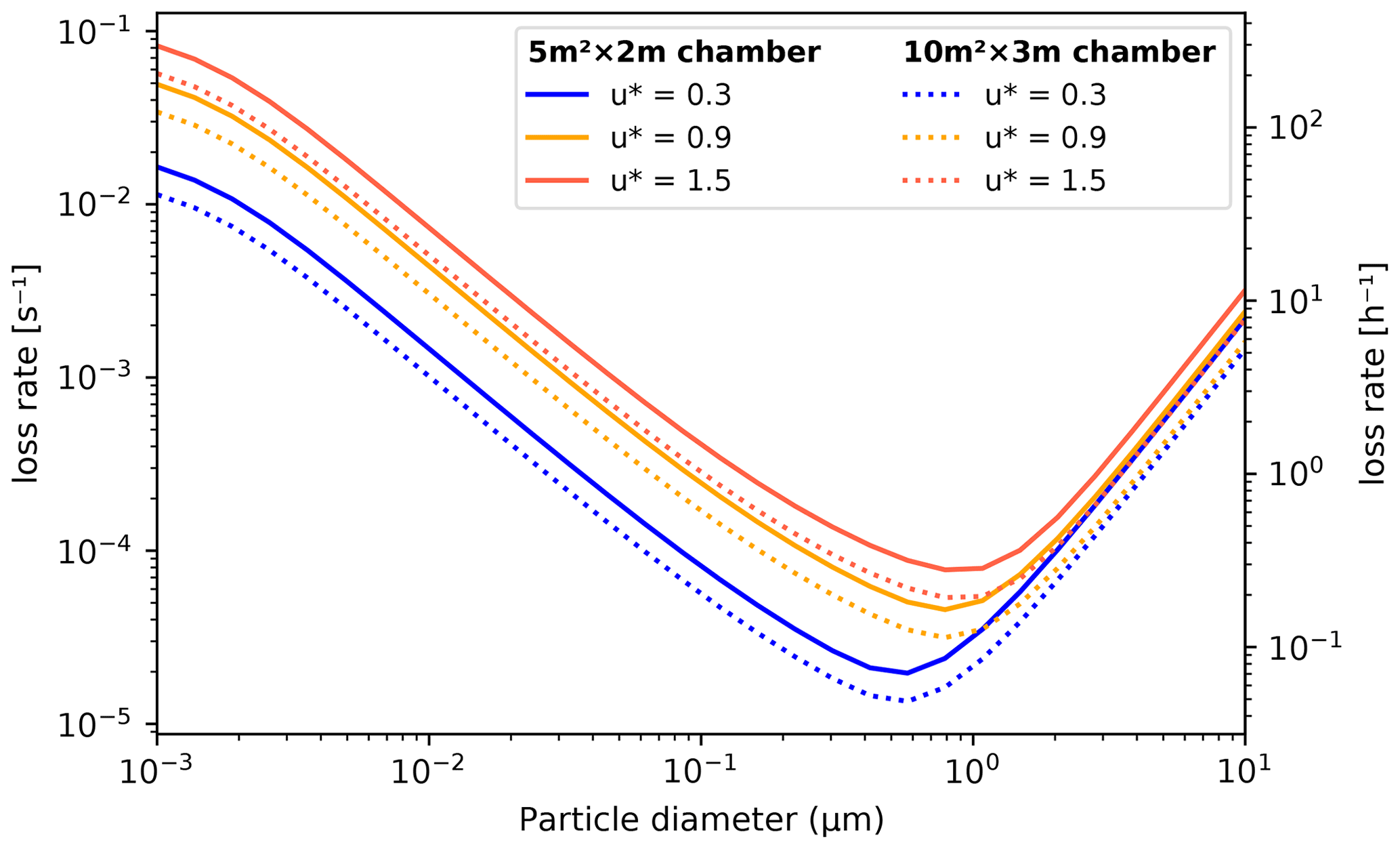
Figure 5Particle loss rates as a function of particle diameter, friction velocity and chamber volume (given as floor area × height) as calculated by the aerosol loss rate parametrization. The rates are calculated at room temperature (20 ∘C) and pressure (1 atm).
The model saves the mass composition of particles lost to walls (in kg m−3) as a cumulative sum. Since the vapour wall losses are reversible, the model saves the mass flux to and from the walls (in , positive value indicates gas to wall flux), calculated as an average over the time interval for saving results.
3.8 Model output
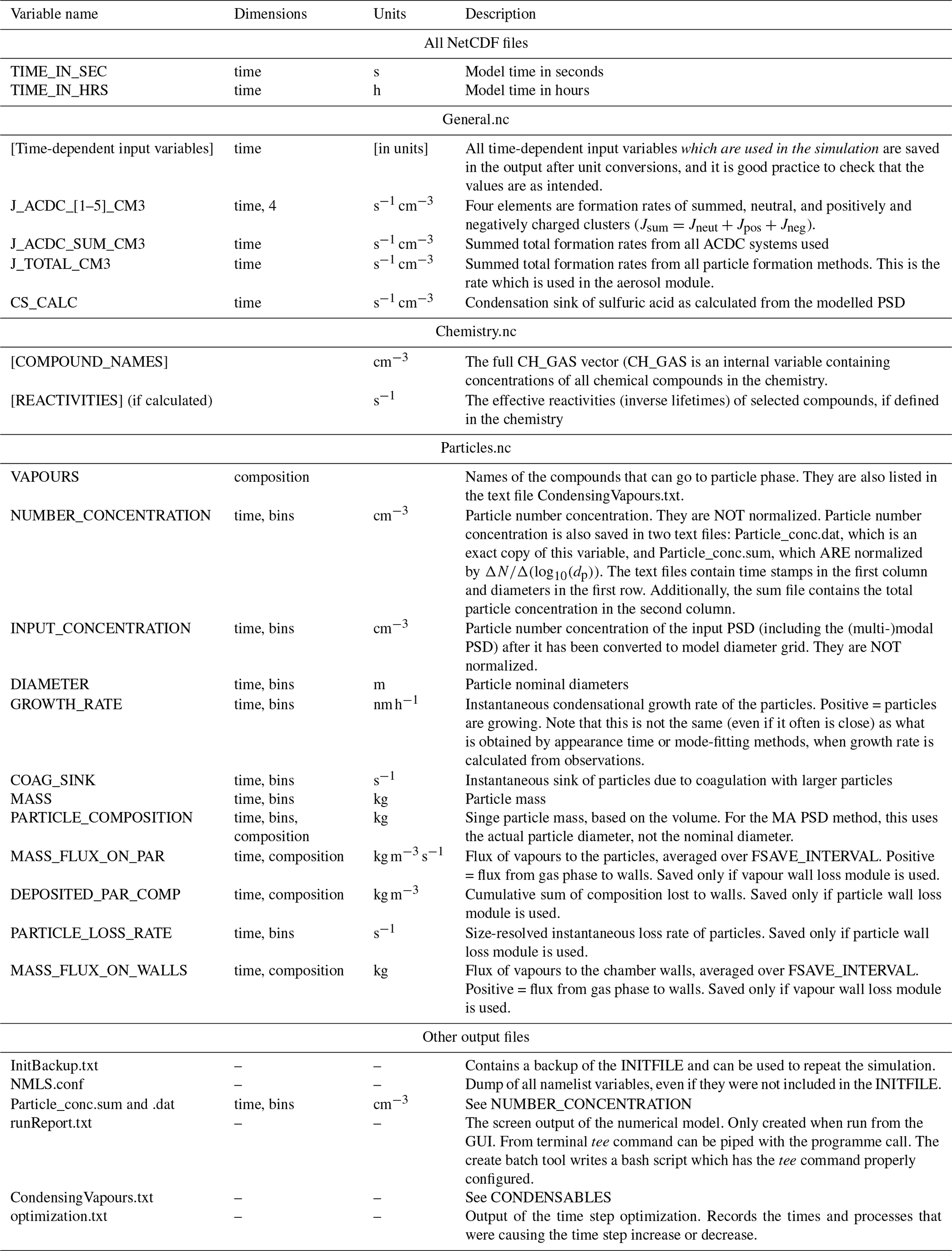
ARCA saves most of the output from the simulations in three compressed NetCDF4 (network common data form) files. The time resolution of the output can be defined in model seconds (FSAVE_INTERVAL) or as number of saved instances (FSAVE_DIVISION). The files contain time series of the environmental variables and nucleation rates and the names of the used ACDC systems (General.nc), gas concentrations of the complete chemical set (Chemistry.nc), and aerosol number concentration, size, coagulation sink, particle growth (by condensation module) and loss rates, vapour concentrations in particle (size-resolved) and gas phase, and the vapour fluxes to and from the particle phase and walls (Particles.nc). All files contain basic attributes of the model configuration, such as the name of the chemistry module used, user-supplied description, name of the output directories and INITFILE, (real) date, and time of the simulation.
When the model is run, a copy the INITFILE which was used to initialize the model is saved (InitBackup.txt). This file can be loaded in the GUI or used as such to repeat the simulation, provided that other input files are the same. A time series of particle number concentrations in normalized and linear scale, as well as a list of condensing vapours, is provided for convenience. If the model was run from the GUI, the screen output of the numerical model is also saved (runReport.txt). A complete list and description of the output variables and files is shown in Table 2.
Table 2Description the output file contents, dimensions and units.
ARCA box has an extensive online user manual (https://wiki.helsinki.fi/display/arca/ARCA+online+manual, last access: 23 September 2022), along with tutorials of installation and example cases. The manual is written completely from the perspective of the user interface, and the underlying scientific base of any procedure is mentioned only if relevant to the instruction. Therefore, we will here introduce the GUI only broadly with a general notion of one possible workflow and emphasize that the user who wishes to learn to use the model should rely on the online user manual. The manual allows the use of many more pictures, videos, interlinking between content and more informal addressing, thus forming a vastly better pedagogical platform for learning than this paper could do.
Typically, a model such as ARCA is used for sensitivity studies and is run multiple times, changing various parameters. It is very easy to lose track of the differences in different simulations, even when the simulation settings are not hardcoded. A user interface is a valuable aid in organizing the model options in a way that helps the user to have a good visual control of the workflow. ARCA's GUI enables this by showing the numerous simulation settings in the relevant context, thus making it easier to check that the input (e.g. units, files, processes in use) are correct by automatizing file and directory naming and creation, by increasing reproducibility with logging and automatic backup of executed simulation settings, by making inspection of the results consistent with the plotting tools tailored for model output, and by providing guidance with direct links to the corresponding page in the online manual, just to name a few examples. While the numerical model is often run directly from the GUI, with a valid INITFILE the compiled Fortran program can always be run from the command line, without the GUI. In fact, this is the best way to use the model in batches of simulations, such as would often be done on a remotely run high-performance computer (HPC).
4.1 GUI design principles
The primary principle of the GUI design has been that the numerical model is kept autonomous of the user interface. This ensures that the model can be run on as many systems as possible, even when the user has no access to a graphical OS, such as when working on a secure shell (SSH) connection to an HPC. Another aspect is that Fortran is a much more conservative language than Python, and it can be expected to work reliably as intended on each OS. While Python is cross-platform, its reliance on multiple extra packages and their rather quick updating schedule make it more susceptible to introduce unintended behaviour in the GUI. While such issues are usually fixed in the ARCA repository quite swiftly, it is highly convenient that the underlying numerical model is working independently of the GUI. The independence between the model and the GUI is ensured through the INITFILE, where the GUI reads and writes a Fortran namelist text file, which is used to initialize the numerical model.
Another design principle has been that the GUI should allow further model development; that is, it should be able to write, save and read in any custom options, even if they are not yet fully incorporated in the graphical layout. Some of these options might be later incorporated, and some may turn out to be unnecessary. This principle manifests itself in the GUI's tab “custom options”.
The third design principle has been to enable flexibility in the input to the model. All input is done via human readable text files. Not all modellers have their input data available in the same units or time resolution, and the GUI lets the user define theirs. However, this flexibility has limits, and in the end the input files are expected to follow a certain structure which is covered in detail in the manual. Also, the example files in the ModelLib directory can be used as a guide.
The last design principle is similar to what any graphical user interface typically aims to do: to collect the options of a program in meaningful groups and hierarchy, showing relevant and hiding unnecessary options, deriving information from user input such as parsing pathnames or calculating values, and providing assistance through help links or tool tips. It can be noted that while the amount of GUI options might seem intimidating, many of them are related to the way the input data are structured, and usually after the initial set up – which takes a while for the first time – the user can leave most options as they are and concentrate on testing further with only a few key options.
4.2 Selected features of the GUI
To give an overview of the GUI, Figs. 6–8 show selected screenshots of the GUI window. For in-depth instructions and descriptions, the user is directed to the online manual, which contains an instructional video and transcript of setting up a simulation with the provided example files. To keep this work concise, here we give a general overview of the key points in setting up a simulation. As an example, we have chosen the case which produces Fig. 11, and whose complete input is included in the directory ModelLib/Examples/APINENE_OXY. Figure 6a shows the tab “general options”, which contains many of the basic options for the simulation: naming of output, paths to input and output files, model time step, and toggles for the main modules. Based on the choices in the “modules in use”, other tabs will be enabled or disabled, and the work procedure is to fill out the “forms” one tab at a time and then use “run ARCA”.

Figure 6Screenshots of the GUI showing the tabs “general input” (a) and “time-dependent input” (b), where the model input concentrations and environmental variables are defined along with their sources and units. The settings shown here are from the simulation shown in Fig. 11.
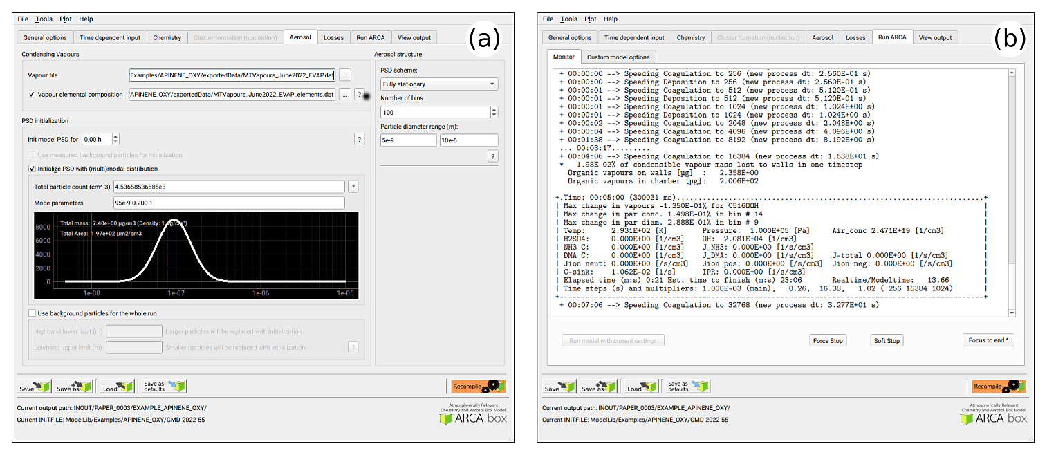
Figure 7Options related to the discrete aerosol module; selection of PSD scheme, number of bins and the size range, and the parametric initial particle size distribution (a), as well as example of the model run-time output (b). The model can be stopped any time forcefully (“force stop”) or gracefully (“soft stop”), in which the latter saves the output gathered so far.
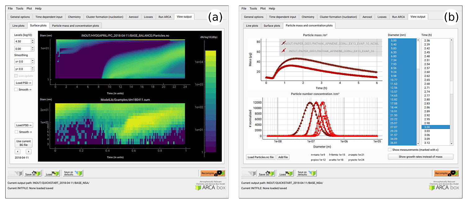
Figure 8Examples of the plotting tools of the model output: surface plots of the modelled (a, top plot) and initialization PSD (a, lower plot). On the right comparison of two simulations, with total particle mass (b, top plot) and size distribution at three time instances (b, lower plot).
After “general options”, the most crucial set of options are in the next tab “time-dependent input” (Fig. 6b). Here the concentrations of precursors and many environmental variables are defined. The logic in this tab is that any other input than temperature and pressure are optional. Any variable which is not defined here as an input will have a constant 0 value. One picks the variables that are given as input to the model from the right-hand panel “available input variables” and moves them to the selected list of input variables. Next, there are several options how to define the values of any variable. For example, O3 could come from measurements, in which case it would be read in from the ENV file from the column number defined in “column/link”, it could be a constant, in which case it would be sufficient to “shift” the default value 0 by the constant amount, or we might want to multiply the measured values by a constant “multi”. Another option would be to link the concentration to some other variable, and then one would use that variable name in “column/link”. Finally, there is a way to use parametric input in the next tab “parametric input”, where a set of sliders can be used to create a smooth time series for any given input variable. This part of setting up the model is usually somewhat time-consuming, but once properly done, the user can easily perform sensitivity tests by using the “shift” and “multi” options of any variable. Furthermore, the tool “variations” can be used for sensitivity tests, which creates a batch of simulations in which any given set of variables are varied within given ranges, containing all combinations of the different input settings.
Figure 7a shows the options related to aerosol module, such as size range and resolution of the PSD grid, its initialization with either measurements from a file or using (multi-)modal lognormal distribution (as is done in this case), and duration and size range of initialization. This tab is also where the pure liquid saturation vapour pressure properties are defined in the “vapour file” and optional “vapour elemental composition” file. In our example case, a single mode log-normal particle size distribution was used to initialize the particles in the simulation. The (multi-)modal PSD is defined by total particle number, mode diameter, standard deviation and relative contribution to the total particle number concentration (PN). The GUI plots the resulting mode in real-time and calculates total particle mass (PM) and particle area, as these are sometimes reported and can be used to fine-tune some unknown modal parameter such as the mode width.
Figure 7b shows an example of the model output during the runtime, when it is used from the GUI. The preferred way of setting up the model the first time is to start the model from the tab “run ARCA” by pressing “run model with current settings” and dealing with the eventual error messages, which might appear due to misconfiguration. If the model enters the main loop (after printing “starting main loop”), it is advisable to press “force stop” and read the initial report of the model that is printed in the “monitor” window. If there are no warning messages, and the reported unit conversions and other reported behaviour corresponds to the intent of the user, the simulation can be performed in full.
Figure 8 shows examples of the output plotting tools such as surface plots (panel a) and particle mass and size distribution plots (panel b). A useful tool is the Live update option, which shows the evolving particle size distribution surface plot during the simulation.
The aim of this section is to verify that the modules in ARCA box perform programmatically as intended. We must stress that the validity of the results of any model is strongly dependent on the input parameters used. Here the reader is reminded of the most crucial parameters in addition to the user-supplied concentrations:
-
for the chemistry module the chemical reaction sets (and accompanying kinetic rate coefficients), spectral data
-
for the formation rate module (ACDC), the Gibbs free energies
-
for condensation and vapour loss modules, the pure liquid saturation vapour pressures.
These are provided in the default ARCA installation as a working example, and while they are from published sources, they are not intended to be used in all conditions and locations. Instead, the user should use the tools in the GUI and online manual to collect and prepare their own set of input parameters and submodules and justify their use based on their simulation conditions. The manual has detailed instructions on how to acquire and format the input data, construct a chemistry module, and update the ACDC systems. The tests shown here are simplified cases whose purpose is to show that the calculations in the model are done correctly. The last test is a comparison against a chamber experiment, which utilizes nearly all the modules and therefore connects all the individual processes. The settings used in this simulation are shown in Appendix C and serve as an example of an INITFILE.
5.1 ACDC
For any given cluster system, the formation rates in ACDC depend largely on the evaporation rates of the clusters, generally calculated from the input Gibbs free energies. Figure 9 shows formation rates calculated with the four ACDC simulation systems: two for H2SO4–NH3 and two for H2SO4–DMA. The systems calculated with the RICC2 (RICC2/aug-cc-pV(T+d)Z//B3LYP/CBSB7) method are described in Olenius et al. (2013) and can be found in the ACDC repository (https://github.com/tolenius/ACDC, last access: 23 September 2022). The DLPNO level NH3 system (DLPNO-CCSD(T)/aug-cc-pVTZ//ωB97X-D/6-31++G**) was used in Besel et al. (2020), whereas the DLPNO DMA system was used in Myllys et al. (2019). Figure 9a shows the significance of ion-mediated clustering in the H2SO4–NH3 system, as is apparent when comparing the total formation rates with and without the presence of ions. It also underlines the already mentioned notion that the charge of the outgrowing clusters does not necessarily correspond to their pathway inside the system. The H2SO4–DMA cluster formation (Fig. 9b) shows weaker sensitivity to the presence of ions.

Figure 9Steady-state particle formation rates from the two H2SO4–NH3 (a) and two H2SO4–DMA systems (b). Both chemistries include data from RICC2 and DLPNO level of theories. Thick lines show the total formation rate, and solid lines are in the presence of ions and dashed lines without ions present. All simulations used the same temperature (5 ∘C) and external cluster losses ( s−1).
5.2 Verification of the coagulation module
The calculations of the Brownian coagulation module were verified in two parts. Figure 10a shows the size-dependent coagulation coefficients calculated by ARCA (for comparison, see Fig. 13.5 in Seinfeld and Pandis, 2016), whereas Fig. 10b compares the evolution of a particle size distribution with an analytical solution to the Brownian coagulation of a polydisperse particle volume distribution. The solution applies the constant, size-independent coagulation coefficient 10−9 (defined by the initial concentration N0=106 cm−3 and characteristic time τc=2000 s), and for this test ARCA's calculated coefficients were replaced with the same constant coagulation coefficient (for comparison, see Fig. 13.6 in Seinfeld and Pandis, 2016). Figure 10 shows that on one hand the coagulation kernel is calculated in the same way as the source but also that the coagulation losses are correctly applied, and therefore the temporal evolution of the discrete particle size distribution in ARCA is identical to an analytical solution of the same initial size distribution.
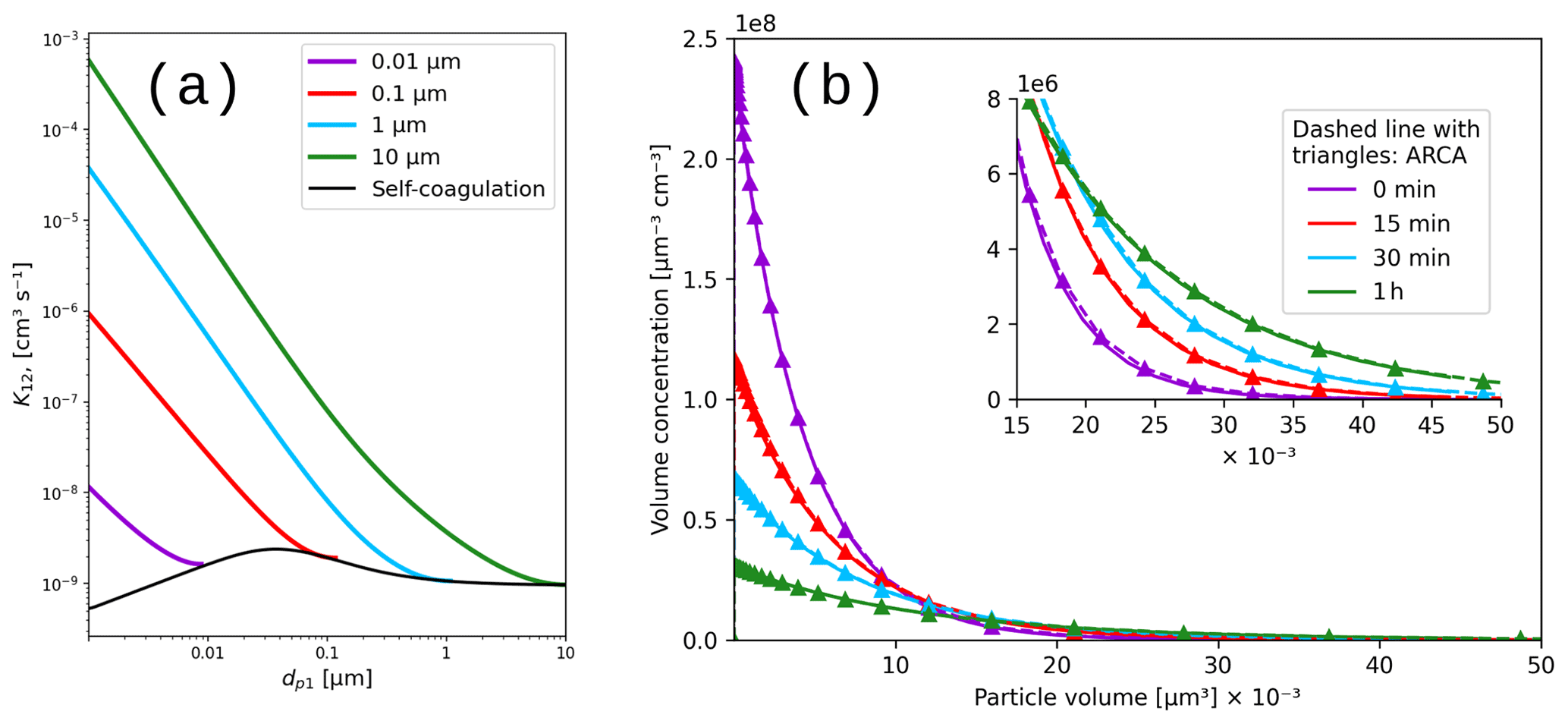
Figure 10Coagulation coefficients used in ARCA box for four different particle diameters (a), with sticking coefficient αg=1. Comparison with analytical coagulation solution (b).
5.3 Chemistry, condensation and loss routines
We simulated α-pinene oxidation in a high-ozone and low-OH chamber environment, similar as in experiment 13 in Pathak et al. (2007) (Fig. 11). The 10 m3 Teflon bag chamber was initially filled with seed particles, α-pinene and 2-butanol as OH scavenger. Then O3 was introduced to the chamber. The reported mean particle loss rate (0.3 h−1) was expanded to size- and time-dependent profiles using Pierce et al. (2008), who measured the losses in the same chamber in more detail. They report an initially higher rate of loss in all their experiments and attribute this to the growth of the particles (leading to slower average loss rate) and to the enhanced loss rate of initially charged seed particles. Since ARCA in its current form does not consider charge effects, we chose to use the reported loss rates with higher initial rate. It means that the simulation is not showing the effect of the loss rate calculated by the particle loss module, but it does still verify that the rates are properly applied – given the good agreement in total particle mass time series. The simulation used moderate wall loss of condensing vapours (, 𝖢𝖶_𝖤𝖰𝖵=40 µm m−3 and 𝖤𝖣𝖣𝖸𝖪=0.05 s−1). The final secondary organic aerosol (SOA) mass yield of 0.169 (final SOA mass/initial α-pinene mass) calculated by ARCA agrees well with the reported 0.17. Without evaporation from the particles, invoked by the accumulation of vapours to walls and the consequential supersaturation decrease, the calculated yield is 0.176. The final concentration of vapours deposited on the walls amounted to 13.4 µg m−3. In the chemistry scheme built for this test, ozone concentration was set to the target (250 ppb) at time 1105 s and was then allowed to evolve according to the chemical reactions. Without chemical wall loss the simulated yield is 0.286, overshooting the reported yield by a factor of 1.7. The pure liquid saturation vapour pressures used were derived using the EVAPORATION method. The chemistry was acquired from MCM and amended with the PRAM, and psat data were downloaded from UManSysProp (http://umansysprop.seaes.manchester.ac.uk, Sect. 3.5), using the tools in ARCA box.
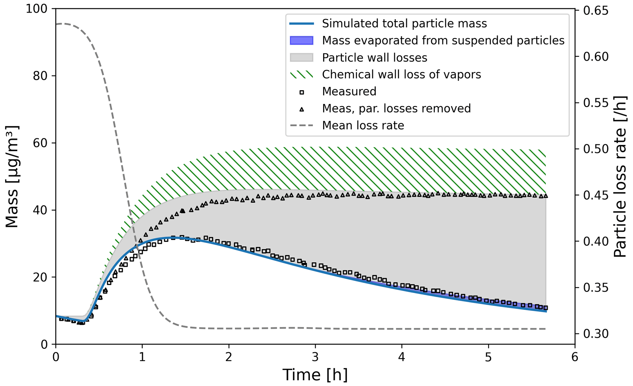
Figure 11Comparison against α-pinene oxidation experiment (exp. 13, Pathak et al., 2007). Size-resolved aerosol wall losses were measured for the same chamber in Pierce et al. (2008). Moderate chemical wall loss is calculated with parametrization from ARCA box using , CW_EQV=40 µm m−3 and EDDYK=0.05 s−1.
The ARCA distribution contains an example case which produces a similar simulation to what was used to produce Fig. 11. Here the initial time without ozone is omitted, and the simulation starts immediately with 250 ppb concentration. To accommodate for the initial particle losses, the initial particle number concentration was set to 4537 cm−3. This simplification makes configuring the model much more straightforward and produces the same result apart from the shift in time when compared with the experiment data.
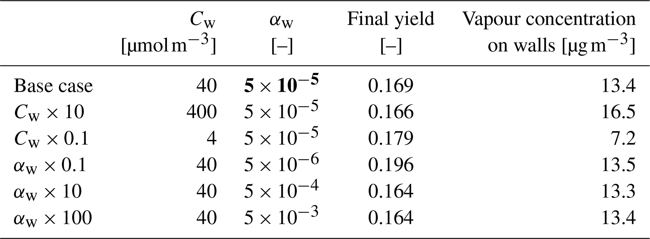
We also performed sensitivity runs where we tested the vapour wall parameters Cw and αw. Changing Cw an order of magnitude lower and higher (to 4 and 400 µm m−3) changed the resulting yield to 0.179 and 0.166, and final total vapour mass on the wall was 7.16 and 16.46 µg m−3, respectively. For reasons discussed in Sect. 3.7 about the limit of very small αw, we saw no practical difference in the yield or vapour mass lost to walls after , where the uptake apparently has become diffusion-limited. The selected default value of αw () can be considered to be close to the value where the surface reactions start playing a role in the uptake.
Table 3Sensitivity of the vapour wall losses to parameters Cw and αw.
6.1 Licensing
ARCA box is licensed under GPL 3.0, and the licensing statements (also those from auxiliary software) are included in the source code. The source code includes software that is not written by authors of ARCA, namely the Fortran DVODE solver (“in the public domain”, or IPD), ACDC (GPL 3) and KPP, which is not strictly necessary for ARCA but provided for convenience (GPL 3), as the original KPP is not able to compile very large chemistry schemes or long variable names.
6.2 System requirements
ARCA's numerical model is written in Fortran and the user interface in Python 3. These environments must be installed and properly working on the computer. Also, since the output data are mainly saved in NetCDF 4 files, this software – along with its Fortran and Python libraries – must be installed prior to compilation and use. ARCA box has been developed on the Linux platform, but due to the cross-platform nature of Python and the availability of Gnu Fortran for all three major OSs, the model has successfully been installed and used on all of them (on Windows GFortran is used through Cygwin and on MacOS through Xcode). The model has not been tested with Intel Fortran, but as it is usually compatible with GFortran, we expect no major issues. The ARCA online manual has step-by-step instructions and videos for the installation of the prerequisite environments, as well as the model itself. It also contains solutions to installation problems which have been reported to us. After the necessary environments are working, installation and compiling the model itself are straightforward with the included Python installer script. The script will install the necessary Python packages (most importantly PyQt5, PyQtGraph, NumPy, Matplotlib and netCDF4) and compile the model.
In its current state, we see ARCA as a robust base, a platform that packages established theories and knowledge of the central processes of this domain in a user-friendly and extendable program. Still, many known processes are for now omitted from the model, and the model will be developed further. This is aided by the fact that ARCA is one of the primary zero-dimensional process models used by the authors.
Current work with model development is concentrating on implementing an inorganic thermodynamic module, similarly as in ADCHEM and ADCHAM (Roldin et al., 2011, 2014). This will enable calculations of size-resolved aerosol hygroscopic growth, acidity (pH) and the saturation concentrations of inorganic acids such as HNO3, HCl and MSA (methanesulfonic acid, CH3SO3H). This information will then be transferred to the condensation/evaporation module which will use the Analytical Predictor of Dissolution (APD) method (Jacobson, 1997b) to solve the gas-particle partitioning. The omission of particle-phase chemistry (organic and inorganic) will affect the suitability of the model in marine air, where a considerable fraction of the aerosol mass is formed through oxidation processes which take place in aqueous phase (Xavier et al., 2022), and with very low concentrations of organic compounds the growth in the model would be almost solely based on the irreversible condensation of sulfuric acid which is formed in the gas-phase chemistry, thus underestimating the total particle mass. Another major constituent of the secondary aerosol mass is nitric acid and ammonium, and these concentrations depend on the water content of the particles. One way to quantify in very broad strokes what a purely gas-phase model is at worst missing would be to look at the measured aerosol composition around the world. Zhang et al. (2007) analysed the submicron aerosol AMS data from 37 field campaigns and found that organic compounds constitute on average 45 % (18 %–70 %), sulfates 32 % (10 %–67 %), nitrates 10 % (1.2 %–28 %), ammonium 13 % (6.9 %–19 %) and chloride 0.6 % (<D.L.–4.8 %); the ranges in parentheses are the ranges between different measurement locations. The current processes in the model are capable of bringing organic molecules, organic nitrates and sulfates (in the form of H2SO4 from SO2 oxidation with OH) to the particle phase, but they would miss ammonium and chlorides. Some fraction of the nitrates and sulfates (and possibly organics too) are resulting from particle-phase reactions in either aqueous form or oligomerization. The effect of particle-phase oxidation of dimethyl sulfide (DMS) and the subsequent formation of methanesulfonic acid (MSA) is one example of a process which is relevant over the oceans (de Jonge et al., 2021) but not necessarily a crucial omission over boreal forest, where similar approaches as in ARCA have been in good agreement with the measured particle mass and size distributions (Roldin et al., 2019).
Another area of improvement is the addition of charged particles, which is a significant factor in chamber wall losses, as was already discussed in Sect. 5.3. These extensions will be available after evaluation in the next version of ARCA. To complement the current particle size distribution methods (FS and MA), we also plan to add a hybrid PSD representation (Chen and Lamb, 1994; Pichelstorfer and Hofmann, 2015). It consists of a fixed size bin grid where the concentrations are described by uniform distributions whose width can vary within each bin. Thus, upon growth or shrinkage, only a fraction of the population is moved to the neighbouring grid cell. This prevents numerical diffusion and avoids “pits” and “peaks” in the PSD output.
ARCA box has already been used and tested by several groups, and the feedback has helped further develop the model and its documentation. The approachable interface and model structure has been a great asset – on one hand it has helped to gain new users, and on the other hand it has helped us to improve the usability and stability, resulting in updates for the whole user community. We are looking forward to the future, when the users of ARCA further participate in the model development by sharing their experience, needs, ideas and even code additions.
The user-definable model options are briefly described here. All options listed here can be defined in the graphical user interface (GUI). We want to emphasize that there is no need to configure ARCA by manually editing the INITFILE. In fact, this would probably lead to unintended outcomes, as some sanity checking of the options is done in the GUI. Additionally, the GUI contains tools, tool tips, help links and visualization of the options. If necessary, for example for model development, the user can also insert any text input to the INITFILE from the GUI, and there is no need to part from the GUI workflow even when an option is not (currently) available in the GUI. All settings, even the raw input, are always saved in the INITFILE written by the GUI and will be available when an INITFILE is loaded in the GUI.
Table A1Model variables which can be set from the GUI and INITFILE. T and F signify true and false, respectively.
Figure B1 shows how the output directory names are formed from the date or index and case and run names, and what files are written in the output directory. The directories are automatically created except for the common out (INOUT_DIR). NetCDF files are binary files and must be read with a compatible software. After installing ARCA, the user has the necessary Python packages to access NetCDF (by “import netCDF4”); other software includes ncdump, Octave, Panoply, etc.
With INITFILE, the model can be run by loading it in the GUI: (1) by drag and drop, (2) ctrl-O, or (3) “load settings”, or it is run from terminal by giving the file path as the command line option:
./arcabox.exe path/to/INITFILE
Example INITFILE used in simulation discussed in Sect. 5.3.
The ARCA model source code, described in this paper, is publicly accessible as a frozen archive (available at https://doi.org/10.5281/zenodo.6787213, Clusius et al., 2022). However, the most recent, constantly updated version is available for download upon request at https://www.helsinki.fi/en/researchgroups/multi-scale-modelling/arca (last access: 26 September 2022). The users are asked to provide their email address and a very brief overview of the intended field of study with ARCA. This information is used to inform us of any future updates, fixes and other news regarding the model, as well as give the ARCA model development group information on the different uses of the model. After the registration the user will be issued a Git pull token to the private GitLab repository. This token can be used later at any point for updating or reinstalling the code.
ARCA's user manual is in Wiki format, found at https://wiki.helsinki.fi/display/arca (last access: 26 September 2022). There are also links from the GUI directly to the relevant parts in the online manual. In addition to the manual, there are tutorial videos and troubleshooting instructions. The manual is updated continuously as the model is further developed, but older states for previous versions are saved in pdf format, available for download at the site.
The data and plotting code used for Figs. 5 and 9–11 are available at https://doi.org/10.5281/zenodo.7002869 (Clusius, 2022).
PC and CX were the principal programmers and jointly coordinated the writing of the numerical model. PC wrote the user manual and the graphical user interface. LP wrote the PSD module and the time step optimization. PZ provided the chemistry modules and the supporting chemistry tools for the user interface. TO provided the ACDC plug-in. PR provided the loss routines. MB wrote the chemistry interface. All authors contributed to the manuscript by way of writing and commenting.
The contact author has declared that none of the authors has any competing interests.
Publisher's note: Copernicus Publications remains neutral with regard to jurisdictional claims in published maps and institutional affiliations.
Petri Clusius and Carlton Xavier share first authorship of this paper. We acknowledge the ACCC Flagship, funded by the Academy of Finland (grant no. 337549), and the computational resources from CSC – IT Center for Science, Finland. Petri Clusius gratefully acknowledges the University of Edinburgh and University of Helsinki Partnership Programme on Forests. Tinja Olenius gratefully acknowledges the Swedish Research Council VR (grant no. 2019-04853) and the Swedish Research Council for Sustainable Development FORMAS (grant no. 2019-01433) for financial support. Pontus Roldin gratefully acknowledges the Swedish Research Council VR (grant no. 2019-05006), the Swedish Research Council for Sustainable Development FORMAS (grant no. 2018-01745), the Crafoord foundation (grant no. 20210969) and the strategic research area MERGE for financial support.
This research has been supported by the Vetenskapsrådet (grant nos. 2019-04853, 2019-01433, 2019-05006, and 2018-01745), the Crafoordska Stiftelsen (grant no. 20210969) and the Academy of Finland (grant no. 337549).
Open-access funding was provided by the Helsinki University Library.
This paper was edited by Christoph Knote and reviewed by two anonymous referees.
Adams, P. J. and Seinfeld, J. H.: Predicting global aerosol size distributions in general circulation models, J. Geophys. Res., 107, AAC 4-1–AAC 4-23, https://doi.org/10.1029/2001jd001010, 2002.
Akherati, A., He, Y., Coggon, M. M., Koss, A. R., Hodshire, A. L., Sekimoto, K., Warneke, C., de Gouw, J., Yee, L., Seinfeld, J. H., Onasch, T. B., Herndon, S. C., Knighton, W. B., Cappa, C. D., Kleeman, M. J., Lim, C. Y., Kroll, J. H., Pierce, J. R., and Jathar, S. H.: Oxygenated Aromatic Compounds are Important Precursors of Secondary Organic Aerosol in Biomass-Burning Emissions, Environ. Sci. Technol., 54, 8568–8579, https://doi.org/10.1021/acs.est.0c01345, 2020.
Almeida, J., Schobesberger, S., Kürten, A., Ortega, I. K., Kupiainen-Määttä, O., Praplan, A. P., Adamov, A., Amorim, A., Bianchi, F., Breitenlechner, M., David, A., Dommen, J., Donahue, N. M., Downard, A., Dunne, E., Duplissy, J., Ehrhart, S., Flagan, R. C., Franchin, A., Guida, R., Hakala, J., Hansel, A., Heinritzi, M., Henschel, H., Jokinen, T., Junninen, H., Kajos, M., Kangasluoma, J., Keskinen, H., Kupc, A., Kurtén, T., Kvashin, A. N., Laaksonen, A., Lehtipalo, K., Leiminger, M., Leppä, J., Loukonen, V., Makhmutov, V., Mathot, S., McGrath, M. J., Nieminen, T., Olenius, T., Onnela, A., Petäjä, T., Riccobono, F., Riipinen, I., Rissanen, M., Rondo, L., Ruuskanen, T., Santos, F. D., Sarnela, N., Schallhart, S., Schnitzhofer, R., Seinfeld, J. H., Simon, M., Sipilä, M., Stozhkov, Y., Stratmann, F., Tomé, A., Tröstl, J., Tsagkogeorgas, G., Vaattovaara, P., Viisanen, Y., Virtanen, A., Vrtala, A., Wagner, P. E., Weingartner, E., Wex, H., Williamson, C., Wimmer, D., Ye, P., Yli-Juuti, T., Carslaw, K. S., Kulmala, M., Curtius, J., Baltensperger, U., Worsnop, D. R., Vehkamäki, H., and Kirkby, J.: Molecular understanding of sulphuric acid–amine particle nucleation in the atmosphere, Nature, 502, 359–363, https://doi.org/10.1038/nature12663, 2013.
Besel, V., Kubečka, J., Kurtén, T., and Vehkamäki, H.: Impact of Quantum Chemistry Parameter Choices and Cluster Distribution Model Settings on Modeled Atmospheric Particle Formation Rates, J. Phys. Chem. A, 124, 5931–5943, https://doi.org/10.1021/acs.jpca.0c03984, 2020.
Bird, R. E. and Riordan, C.: Simple Solar Spectral Model for Direct and Diffuse Irradiance on Horizontal and Tilted Planes at the Earth's Surface for Cloudless Atmospheres, J. Appl. Meteorol. Clim., 25, 87–97, https://doi.org/10.1175/1520-0450(1986)025<0087:sssmfd>2.0.co;2, 1986.
Boy, M. and Kulmala, M.: The part of the solar spectrum with the highest influence on the formation of SOA in the continental boundary layer, Atmos. Chem. Phys., 2, 375–386, https://doi.org/10.5194/acp-2-375-2002, 2002.
Boy, M., Hellmuth, O., Korhonen, H., Nilsson, E. D., ReVelle, D., Turnipseed, A., Arnold, F., and Kulmala, M.: MALTE – model to predict new aerosol formation in the lower troposphere, Atmos. Chem. Phys., 6, 4499–4517, https://doi.org/10.5194/acp-6-4499-2006, 2006.
Boy, M., Sogachev, A., Lauros, J., Zhou, L., Guenther, A., and Smolander, S.: SOSA – a new model to simulate the concentrations of organic vapours and sulphuric acid inside the ABL – Part 1: Model description and initial evaluation, Atmos. Chem. Phys., 11, 43–51, https://doi.org/10.5194/acp-11-43-2011, 2011.
Boy, M., Mogensen, D., Smolander, S., Zhou, L., Nieminen, T., Paasonen, P., Plass-Dülmer, C., Sipilä, M., Petäjä, T., Mauldin, L., Berresheim, H., and Kulmala, M.: Oxidation of SO2 by stabilized Criegee intermediate (sCI) radicals as a crucial source for atmospheric sulfuric acid concentrations, Atmos. Chem. Phys., 13, 3865–3879, https://doi.org/10.5194/acp-13-3865-2013, 2013.
Bruun, H. H.: Hot-Wire Anemometry: Principles and Signal Analysis, Oxford University Press, Oxford, UK, ISBN 978-0-198-56342-6, 1995.
Chen, J.-P. and Lamb, D.: Simulation of Cloud Microphysical and Chemical Processes Using a Multicomponent Framework. Part I: Description of the Microphysical Model, J. Atmos. Sci., 51, 2613–2630, https://doi.org/10.1175/1520-0469(1994)051<2613:socmac>2.0.co;2, 1994.
Clusius P.: Dataset in GMD-2022-55 (Version 1), Zenodo [data set], https://doi.org/10.5281/zenodo.7002869, 2022.
Clusius P., Xavier C., Pichelstorfer L., Zhou P., Olenius T., Roldin P., and Boy M.: Atmospherically relevant chemistry and aerosol box model – ARCA box (version 1.2.2), Zenodo [code], https://doi.org/10.5281/zenodo.6787213, 2022.
Compernolle, S., Ceulemans, K., and Müller, J.-F.: EVAPORATION: a new vapour pressure estimation methodfor organic molecules including non-additivity and intramolecular interactions, Atmos. Chem. Phys., 11, 9431–9450, https://doi.org/10.5194/acp-11-9431-2011, 2011.
Daescu, D., Sandu, A., and Carmichael, G. R.: Direct and Adjoint Sensitivity Analysis of Chemical Kinetic Systems with KPP: II – Validation and Numerical Experiments, Atmos. Environ., 37, 5097–5114, 2003.
Damian, V., Sandu, A., Damian, M., Potra, F., and Carmichael, G. R.: The kinetic preprocessor KPP-a software environment for solving chemical kinetics, Comput. Chem. Eng., 26, 1567–1579, https://doi.org/10.1016/s0098-1354(02)00128-x, 2002.
Eckert, F. and Klamt, A.: Fast solvent screening via quantum chemistry: COSMO-RS approach, AIChE J., 48, 369–385, https://doi.org/10.1002/aic.690480220, 2002.
Fuchs, N. A.: The mechanics of aerosols, Pergamon Press, London, https://doi.org/10.1002/qj.49709138822, 1964.
Gelbard, F. and Seinfeld, J. H.: Simulation of multicomponent aerosol dynamics, J. Colloid Interf. Sci., 78, 485–501, https://doi.org/10.1016/0021-9797(80)90587-1, 1980.
Jacobson, M. Z.: Development and application of a new air pollution modeling system – II. Aerosol module structure and design, Atmos. Environ., 31, 131–144, https://doi.org/10.1016/1352-2310(96)00202-6, 1997a.
Jacobson, M. Z.: Numerical Techniques to Solve Condensational and Dissolutional Growth Equations When Growth is Coupled to Reversible Reactions, Aerosol Sci. Tech., 27, 491–498, https://doi.org/10.1080/02786829708965489, 1997b.
Jacobson, M. Z.: Analysis of aerosol interactions with numerical techniques for solving coagulation, nucleation, condensation, dissolution, and reversible chemistry among multiple size distributions, J. Geophys. Res., 107, AAC 2-1–AAC 2-23, https://doi.org/10.1029/2001jd002044, 2002.
Jacobson, M. Z.: Fundamentals of Atmospheric Modeling, 2nd edn., Cambridge University Press, https://doi.org/10.1017/cbo9781139165389, 2005.
Jenkin, M. E., Saunders, S. M., and Pilling, M. J.: The tropospheric degradation of volatile organic compounds: a protocol for mechanism development, Atmos. Environ., 31, 81–104, https://doi.org/10.1016/s1352-2310(96)00105-7, 1997.
Jenkin, M. E., Young, J. C., and Rickard, A. R.: The MCM v3.3.1 degradation scheme for isoprene, Atmos. Chem. Phys., 15, 11433–11459, https://doi.org/10.5194/acp-15-11433-2015, 2015.
Karl, M., Pirjola, L., Grönholm, T., Kurppa, M., Anand, S., Zhang, X., Held, A., Sander, R., Dal Maso, M., Topping, D., Jiang, S., Kangas, L., and Kukkonen, J.: Description and evaluation of the community aerosol dynamics model MAFOR v2.0, Geosci. Model Dev., 15, 3969–4026, https://doi.org/10.5194/gmd-15-3969-2022, 2022.
Kokkola, H., Kühn, T., Laakso, A., Bergman, T., Lehtinen, K. E. J., Mielonen, T., Arola, A., Stadtler, S., Korhonen, H., Ferrachat, S., Lohmann, U., Neubauer, D., Tegen, I., Siegenthaler-Le Drian, C., Schultz, M. G., Bey, I., Stier, P., Daskalakis, N., Heald, C. L., and Romakkaniemi, S.: SALSA2.0: The sectional aerosol module of the aerosol–chemistry–climate model ECHAM6.3.0-HAM2.3-MOZ1.0, Geosci. Model Dev., 11, 3833–3863, https://doi.org/10.5194/gmd-11-3833-2018, 2018.
Kürten, A., Bianchi, F., Almeida, J., Kupiainen-Määttä, O., Dunne, E. M., Duplissy, J., Williamson, C., Barmet, P., Breitenlechner, M., Dommen, J., Donahue, N. M., Flagan, R. C., Franchin, A., Gordon, H., Hakala, J., Hansel, A., Heinritzi, M., Ickes, L., Jokinen, T., Kangasluoma, J., Kim, J., Kirkby, J., Kupc, A., Lehtipalo, K., Leiminger, M., Makhmutov, V., Onnela, A., Ortega, I. K., Petäjä, T., Praplan, A. P., Riccobono, F., Rissanen, M. P., Rondo, L., Schnitzhofer, R., Schobesberger, S., Smith, J. N., Steiner, G., Stozhkov, Y., Tomé, A., Tröstl, J., Tsagkogeorgas, G., Wagner, P. E., Wimmer, D., Ye, P., Baltensperger, U., Carslaw, K., Kulmala, M., and Curtius, J.: Experimental particle formation rates spanning tropospheric sulfuric acid and ammonia abundances, ion production rates, and temperatures, J. Geophys. Res.-Atmos., 121, 12377–12400, https://doi.org/10.1002/2015jd023908, 2016.
Kurtén, T., Tiusanen, K., Roldin, P., Rissanen, M., Luy, J.-N., Boy, M., Ehn, M., and Donahue, N.: α-Pinene Autoxidation Products May Not Have Extremely Low Saturation Vapor Pressures Despite High O:C Ratios, J. Phys. Chem. A, 120, 2569–2582, https://doi.org/10.1021/acs.jpca.6b02196, 2016.
Kylling, A., Webb, A. R., Bais, A. F., Blumthaler, M., Schmitt, R., Thiel, S., Kazantzidis, A., Kift, R., Misslbeck, M., Schallhart, B., Schreder, J., Topaloglou, C., Kazadzis, S., and Rimmer, J.: Actinic flux determination from measurements of irradiance, J. Geophys. Res., 108, ACH 11-1–ACH 11-10, https://doi.org/10.1029/2002jd003236, 2003.
Lai, A. C. K. and Nazaroff, W. W.: Modeling indoor particle deposition from turbulent flow onto smooth surfaces, J. Aerosol Sci., 31, 463–476, https://doi.org/10.1016/S0021-8502(99)00536-4, 2000.
Lehtinen, K. E., Maso, M. D., Kulmala, M., and Kerminen, V.-M.: Estimating nucleation rates from apparent particle formation rates and vice versa: Revised formulation of the Kerminen–Kulmala equation, J. Aerosol Sci., 38, 988–994, https://doi.org/10.1016/j.jaerosci.2007.06.009, 2007.
Matsunaga, A. and Ziemann, P. J.: Gas-Wall Partitioning of Organic Compounds in a Teflon Film Chamber and Potential Effects on Reaction Product and Aerosol Yield Measurements, Aerosol Sci. Tech., 44, 881–892, https://doi.org/10.1080/02786826.2010.501044, 2010.
McGrath, M. J., Olenius, T., Ortega, I. K., Loukonen, V., Paasonen, P., Kurtén, T., Kulmala, M., and Vehkamäki, H.: Atmospheric Cluster Dynamics Code: a flexible method for solution of the birth-death equations, Atmos. Chem. Phys., 12, 2345–2355, https://doi.org/10.5194/acp-12-2345-2012, 2012.
McMurry, P. H. and Grosjean, D.: Gas and aerosol wall losses in Teflon film smog chambers, Environ. Sci. Technol., 19, 1176–1182, https://doi.org/10.1021/es00142a006, 1985.
Mohs, A. J. and Bowman, F. M.: Eliminating Numerical Artifacts When Presenting Moving Center Sectional Aerosol Size Distributions, Aerosol Air Qual. Res., 11, 21–30, https://doi.org/10.4209/aaqr.2010.06.0046, 2011.
Myllys, N., Kubečka, J., Besel, V., Alfaouri, D., Olenius, T., Smith, J. N., and Passananti, M.: Role of base strength, cluster structure and charge in sulfuric-acid-driven particle formation, Atmos. Chem. Phys., 19, 9753–9768, https://doi.org/10.5194/acp-19-9753-2019, 2019.
Nannoolal, Y., Rarey, J., and Ramjugernath, D.: Estimation of pure component properties, Fluid Phase Equilibr., 269, 117–133, https://doi.org/10.1016/j.fluid.2008.04.020, 2008.
O'Meara, S. P., Xu, S., Topping, D., Alfarra, M. R., Capes, G., Lowe, D., Shao, Y., and McFiggans, G.: PyCHAM (v2.1.1): a Python box model for simulating aerosol chambers, Geosci. Model Dev., 14, 675–702, https://doi.org/10.5194/gmd-14-675-2021, 2021.
Olenius, T., Kupiainen-Määttä, O., Ortega, I. K., Kurtén, T., and Vehkamäki, H.: Free energy barrier in the growth of sulfuric acid–ammonia and sulfuric acid–dimethylamine clusters, J. Chem. Phys., 139, 084312, https://doi.org/10.1063/1.4819024, 2013.
O'Meara, S., Booth, A. M., Barley, M. H., Topping, D., and McFiggans, G.: An assessment of vapour pressure estimation methods, Phys. Chem. Chem. Phys., 16, 19453–19469, https://doi.org/10.1039/c4cp00857j, 2014.
Ortega, I. K., Kupiainen, O., Kurtén, T., Olenius, T., Wilkman, O., McGrath, M. J., Loukonen, V., and Vehkamäki, H.: From quantum chemical formation free energies to evaporation rates, Atmos. Chem. Phys., 12, 225–235, https://doi.org/10.5194/acp-12-225-2012, 2012.
Paasonen, P., Nieminen, T., Asmi, E., Manninen, H. E., Petäjä, T., Plass-Dülmer, C., Flentje, H., Birmili, W., Wiedensohler, A., Hõrrak, U., Metzger, A., Hamed, A., Laaksonen, A., Facchini, M. C., Kerminen, V.-M., and Kulmala, M.: On the roles of sulphuric acid and low-volatility organic vapours in the initial steps of atmospheric new particle formation, Atmos. Chem. Phys., 10, 11223–11242, https://doi.org/10.5194/acp-10-11223-2010, 2010.
Pankow, J. F.: An absorption model of gas/particle partitioning of organic compounds in the atmosphere, Atmos. Environ., 28, 185–188, https://doi.org/10.1016/1352-2310(94)90093-0, 1994.
Pankow, J. F. and Asher, W. E.: SIMPOL.1: a simple group contribution method for predicting vapor pressures and enthalpies of vaporization of multifunctional organic compounds, Atmos. Chem. Phys., 8, 2773–2796, https://doi.org/10.5194/acp-8-2773-2008, 2008.
Pathak, R. K., Stanier, C. O., Donahue, N. M., and Pandis, S. N.: Ozonolysis of α-pinene at atmospherically relevant concentrations: Temperature dependence of aerosol mass fractions (yields), J. Geophys. Res., 112, D03201, https://doi.org/10.1029/2006jd007436, 2007.
Peng, Z. and Jimenez, J. L.: KinSim: A Research-Grade, User-Friendly, Visual Kinetics Simulator for Chemical-Kinetics and Environmental-Chemistry Teaching, J. Chem. Educ., 96, 806–811, https://doi.org/10.1021/acs.jchemed.9b00033, 2019.
Pichelstorfer, L. and Hofmann, W.: Modeling aerosol dynamics of cigarette smoke in a denuder tube, J. Aerosol Sci., 88, 72–89, https://doi.org/10.1016/j.jaerosci.2015.05.009, 2015.
Pichelstorfer, L., Winkler-Heil, R., Boy, M., and Hofmann, W.: Aerosol dynamics simulations of the anatomical variability of e-cigarette particle and vapor deposition in a stochastic lung, J. Aerosol Sci., 158, 105706, https://doi.org/10.1016/j.jaerosci.2020.105706, 2021.
Pierce, J. R., Engelhart, G. J., Hildebrandt, L., Weitkamp, E. A., Pathak, R. K., Donahue, N. M., Robinson, A. L., Adams, P. J., and Pandis, S. N.: Constraining Particle Evolution from Wall Losses, Coagulation, and Condensation-Evaporation in Smog-Chamber Experiments: Optimal Estimation Based on Size Distribution Measurements, Aerosol Sci. Tech., 42, 1001–1015, https://doi.org/10.1080/02786820802389251, 2008.
Riipinen, I., Pierce, J. R., Donahue, N. M., and Pandis, S. N.: Equilibration time scales of organic aerosol inside thermodenuders: Evaporation kinetics versus thermodynamics, Atmos. Environ., 44, 597–607, https://doi.org/10.1016/j.atmosenv.2009.11.022, 2010.
Roldin, P., Swietlicki, E., Schurgers, G., Arneth, A., Lehtinen, K. E. J., Boy, M., and Kulmala, M.: Development and evaluation of the aerosol dynamics and gas phase chemistry model ADCHEM, Atmos. Chem. Phys., 11, 5867–5896, https://doi.org/10.5194/acp-11-5867-2011, 2011.
Roldin, P., Eriksson, A. C., Nordin, E. Z., Hermansson, E., Mogensen, D., Rusanen, A., Boy, M., Swietlicki, E., Svenningsson, B., Zelenyuk, A., and Pagels, J.: Modelling non-equilibrium secondary organic aerosol formation and evaporation with the aerosol dynamics, gas- and particle-phase chemistry kinetic multilayer model ADCHAM, Atmos. Chem. Phys., 14, 7953–7993, https://doi.org/10.5194/acp-14-7953-2014, 2014.
Roldin, P., Ehn, M., Kurtén, T., Olenius, T., Rissanen, M. P., Sarnela, N., Elm, J., Rantala, P., Hao, L., Hyttinen, N., Heikkinen, L., Worsnop, D. R., Pichelstorfer, L., Xavier, C., Clusius, P., Öström, E., Petäjä, T., Kulmala, M., Vehkamäki, H., Virtanen, A., Riipinen, I., and Boy, M.: The role of highly oxygenated organic molecules in the Boreal aerosol-cloud-climate system, Nat. Commun., 10, 4370, https://doi.org/10.1038/s41467-019-12338-8, 2019.
Rose, C., Chaumerliac, N., Deguillaume, L., Perroux, H., Mouchel-Vallon, C., Leriche, M., Patryl, L., and Armand, P.: Modeling the partitioning of organic chemical species in cloud phases with CLEPS (1.1), Atmos. Chem. Phys., 18, 2225–2242, https://doi.org/10.5194/acp-18-2225-2018, 2018.
Sandu, A., Verwer, J., Blom, J., Spee, E., Carmichael, G., and Potra, F.: Benchmarking stiff ode solvers for atmospheric chemistry problems II: Rosenbrock solvers, Atmos. Environ., 31, 3459–3472, https://doi.org/10.1016/s1352-2310(97)83212-8, 1997.
Sandu, A., Daescu, D., and Carmichael, G.R.: Direct and Adjoint Sensitivity Analysis of Chemical Kinetic Systems with KPP: I – Theory and Software Tools, Atmos. Environ., 37, 5083–5096, 2003.
Saunders, S. M., Jenkin, M. E., Derwent, R. G., and Pilling, M. J.: Protocol for the development of the Master Chemical Mechanism, MCM v3 (Part A): tropospheric degradation of non-aromatic volatile organic compounds, Atmos. Chem. Phys., 3, 161–180, https://doi.org/10.5194/acp-3-161-2003, 2003.
Seinfeld, J. H. and Pandis, S. N.: Atmospheric Chemistry and Physics – From Air Pollution to Climate Change, 3rd edn., Wiley-Interscience, ISBN: 978-1-118-94740-1, 2016.
Shiraiwa, M., Pfrang, C., and Pöschl, U.: Kinetic multi-layer model of aerosol surface and bulk chemistry (KM-SUB): the influence of interfacial transport and bulk diffusion on the oxidation of oleic acid by ozone, Atmos. Chem. Phys., 10, 3673–3691, https://doi.org/10.5194/acp-10-3673-2010, 2010.
Smith, J. N., Draper, D. C., Chee, S., Dam, M., Glicker, H., Myers, D., Thomas, A. E., Lawler, M. J., and Myllys, N.: Atmospheric clusters to nanoparticles: Recent progress and challenges in closing the gap in chemical composition, J. Aerosol Sci., 153, 105733, https://doi.org/10.1016/j.jaerosci.2020.105733, 2021.
Su, T. and Chesnavich, W. J.: Parametrization of the ion–polar molecule collision rate constant by trajectory calculations, J. Chem. Phys., 76, 5183–5185, https://doi.org/10.1063/1.442828, 1982.
Topping, D., Connolly, P., and Reid, J.: PyBox: An automated box-model generator for atmospheric chemistry and aerosol simulations, Journal of Open Source Software, 3, 755, https://doi.org/10.21105/joss.00755, 2018.
Tsang, T. H. and Brock, J. R.: Simulation of Condensation Aerosol Growth by Condensation and Evaporation, Aerosol Sci. Tech., 2, 311–320, https://doi.org/10.1080/02786828308958637, 1982.
Valorso, R., Aumont, B., Camredon, M., Raventos-Duran, T., Mouchel-Vallon, C., Ng, N. L., Seinfeld, J. H., Lee-Taylor, J., and Madronich, S.: Explicit modelling of SOA formation from α-pinene photooxidation: sensitivity to vapour pressure estimation, Atmos. Chem. Phys., 11, 6895–6910, https://doi.org/10.5194/acp-11-6895-2011, 2011.
Vignati, E., Wilson, J., and Stier, P.: M7: An efficient size-resolved aerosol microphysics module for large-scale aerosol transport models, J. Geophys. Res.-Atmos., 109, D22202, https://doi.org/10.1029/2003jd004485, 2004.
von Smoluchowski, M.: Versuch einer mathematischen Theorie der Koagulationskinetik kolloider Lösungen, Z. Phys. Chem., 92U, 129–168, https://doi.org/10.1515/zpch-1918-9209, 1918.
Wagner, P. E.: Topics in Current Physics, in: Aerosol Microphysics II: Chemical Physics of Microparticles, edited by: Marlow, W. H., Springer, Berlin, Heidelberg, 129–178, https://doi.org/10.1007/978-3-642-81805-9_5, 1982.
Whitby, E. R. and McMurry, P. H.: Modal Aerosol Dynamics Modeling, Aerosol Sci. Tech., 27, 673–688, https://doi.org/10.1080/02786829708965504, 1997.
Wollesen de Jonge, R., Elm, J., Rosati, B., Christiansen, S., Hyttinen, N., Lüdemann, D., Bilde, M., and Roldin, P.: Secondary aerosol formation from dimethyl sulfide – improved mechanistic understanding based on smog chamber experiments and modelling, Atmos. Chem. Phys., 21, 9955–9976, https://doi.org/10.5194/acp-21-9955-2021, 2021.
Xavier, C., Rusanen, A., Zhou, P., Dean, C., Pichelstorfer, L., Roldin, P., and Boy, M.: Aerosol mass yields of selected biogenic volatile organic compounds – a theoretical study with nearly explicit gas-phase chemistry, Atmos. Chem. Phys., 19, 13741–13758, https://doi.org/10.5194/acp-19-13741-2019, 2019.
Xavier, C., Baykara, M., Wollesen de Jonge, R., Altstädter, B., Clusius, P., Vakkari, V., Thakur, R., Beck, L., Becagli, S., Severi, M., Traversi, R., Krejci, R., Tunved, P., Mazzola, M., Wehner, B., Sipilä, M., Kulmala, M., Boy, M., and Roldin, P.: Secondary aerosol formation in marine Arctic environments: a model measurement comparison at Ny-Ålesund, Atmos. Chem. Phys., 22, 10023–10043, https://doi.org/10.5194/acp-22-10023-2022, 2022.
Yli-Juuti, T., Barsanti, K., Hildebrandt Ruiz, L., Kieloaho, A.-J., Makkonen, U., Petäjä, T., Ruuskanen, T., Kulmala, M., and Riipinen, I.: Model for acid-base chemistry in nanoparticle growth (MABNAG), Atmos. Chem. Phys., 13, 12507–12524, https://doi.org/10.5194/acp-13-12507-2013, 2013.
Zhang, Q., Jimenez, J. L., Canagaratna, M. R., Allan, J. D., Coe, H., Ulbrich, I., Alfarra, M. R., Takami, A., Middlebrook, A. M., Sun, Y. L., Dzepina, K., Dunlea, E., Docherty, K., DeCarlo, P. F., Salcedo, D., Onasch, T., Jayne, J. T., Miyoshi, T., Shimono, A., Hatakeyama, S., Takegawa, N., Kondo, Y., Schneider, J., Drewnick, F., Borrmann, S., Weimer, S., Demerjian, K., Williams, P., Bower, K., Bahreini, R., Cottrell, L., Griffin, R. J., Rautiainen, J., Sun, J. Y., Zhang, Y. M., and Worsnop, D. R.: Ubiquity and dominance of oxygenated species in organic aerosols in anthropogenically-influenced Northern Hemisphere midlatitudes, Geophys. Res. Lett., 34, L13801, https://doi.org/10.1029/2007gl029979, 2007.
Zhang, X., Cappa, C. D., Jathar, S. H., McVay, R. C., Ensberg, J. J., Kleeman, M. J., and Seinfeld, J. H.: Influence of vapor wall loss in laboratory chambers on yields of secondary organic aerosol, P. Natl. Acad. Sci. USA, 111, 5802–5807, https://doi.org/10.1073/pnas.1404727111, 2014.
Zhang, Y., Seigneur, C., Seinfeld, J. H., Jacobson, M. Z., and Binkowski, F. S.: Simulation of Aerosol Dynamics: A Comparative Review of Algorithms Used in Air Quality Models, Aerosol Sci. Tech., 31, 487–514, https://doi.org/10.1080/027868299304039, 1999.
- Abstract
- Introduction
- Scope and uses of the ARCA box
- Modules of ARCA box and their theoretical base
- Using the model – graphical user interface (GUI)
- Verification and evaluation of main modules
- Technical information of ARCA box
- Current limitations and future developments
- Appendix A: List of variables used in the INITFILE
- Appendix B: Output files, variables and folder structure
- Appendix C: INITFILE
- Code availability
- Data availability
- Author contributions
- Competing interests
- Disclaimer
- Acknowledgements
- Financial support
- Review statement
- References