Modeling Indian Ocean circulation to study marine debris dispersion: insights into high-resolution and wave forcing effects with Symphonie 3.6.6

The Indian Ocean basin faces significant anthropogenic pressure due to its connection to over 2.2 billion people through river basins. Indian Ocean dynamics are characterized by strong regional and seasonal variability driven by the monsoon system and intense eddy activity. To support future studies on land-sea transfers and marine debris dispersion in this complex ocean, we developed a new circulation modeling configuration using the hydrodynamic model SYMPHONIE. Our configuration introduces a unique telescopic grid covering the entire basin, enabling the study of sub-basin connectivity while resolving meso and submesoscale processes in the coastal region, from the Mozambique Channel to the Bay of Bengal, at a resolution of 1 to 3 km. Additionally, we integrate the recently released high-resolution GloFAS river discharge dataset to force the physical simulations with daily freshwater inputs. Three annual experiments are conducted, exploring the effects of wave forcing and spatial resolution. The reference simulation (IndOc.HR) uses high resolution without wave forcing, IndOc.HR-Sto uses the same resolution but includes wave forcing through both the Stokes-Coriolis force and the Stokes drift, and IndOc.12 is a lower-resolution simulation without wave forcing. Comparisons of temperature, salinity and sea level with in situ and satellite data show the good performance of the simulations and the ability of the high resolution model to accurately capture the spatial and temporal variability of surface dynamics and water masses over the Indian Ocean. We further analyze energy budgets and perform Lagrangian experiments to illustrate the critical role of resolution and waves in shaping the circulation and the resulting marine debris dispersion patterns. The effect of energy levels is particularly significant on trajectory statistics such as average travel distances and preferred spread direction. Notably, Stokes drift has a significant seasonal effect in the Arabian Sea during the southwest monsoon, while current field resolution strongly influences trajectories in the Mozambique Channel. Our results provide a robust modeling framework for studying Indian Ocean dynamics and exploring their effect on marine connectivity and the transport of matter, including pollutants, larvae or organic matter.

1 Introduction

The Indian Ocean is characterized by complex atmospheric and oceanic dynamics that influence marine debris dispersion and connectivity (Pattiaratchi et al., 2022). Its circulation is marked by a strong regional variability and subject to rapid warming and marine heatwaves (Phillips et al., 2021). In the northern hemisphere, the reversal of the monsoon-driven currents between seasons results in significant exchanges between the Arabian Sea and the Bay of Bengal, with potentially high stranding rates of marine debris along the coasts (van der Mheen et al., 2020). In the south, large quantities of debris are trapped in the subtropical gyre (Thibault et al., 2024) connected to the other southern hemisphere gyres of the Atlantic and Pacific Oceans through the Agulhas and Tasman leakages (Maes et al., 2018; Qu et al., 2019; Dobler et al., 2019). However, the general patterns of dispersion and accumulation in this basin remain debated and under-studied (Pattiaratchi et al., 2022). In addition to this large-scale regional circulation, buoyant materials are concentrated by horizontal density fronts and mesoscale cyclonic activity (D'Asaro et al., 2018; Vic et al., 2022). Such frontal zones generate submesoscale structures and filaments, which actively converge drifting particles towards highly concentrated areas (Lodise et al., 2020; Weiss et al., 2024a). Submesoscale convergences are associated with higher vertical velocities than those found in mesoscale fronts, potentially enhancing mixing and accelerating spreading (D'Asaro et al., 2018; Lodise et al., 2020). But submesoscale features are ephemeral, and the clustering of marine debris in such structures may occur over a few to 10 d before slowly dissipating (D'Asaro et al., 2018). In a contamination monitoring context, understanding and interpreting convergence phenomena is challenging due to the short timescales involved. This is especially true in the case of plastic pollution, where the complexity of sampling and quantification makes it currently very difficult to verify the model-based hypotheses. Due to the scarcity of plastic debris concentration data in the ocean, it is currently impossible to capture the spatial and temporal variability of accumulation processes and concentration gradients associated with meso and submesoscales from observations.

Lagrangian dispersion modeling studies can help to fill this knowledge gap. They need in particular to be based on realistic current fields with grid resolutions permitting the representation of such structures and processes at different scales. In recent studies however, the finest horizontal resolutions achieved in ocean simulations over the entire Indian Basin available for Lagrangian scenarios range from $\mathrm{1}/\mathrm{4}$ to $\mathrm{1}/\mathrm{12}$° (∼ 25 to 9 km), based on various configurations of global hydrodynamic models and products: the $\mathrm{1}/\mathrm{12}$° CMEMS Global Ocean Physics Reanalysis GLORYS12V1 (Lellouche et al., 2021), the $\mathrm{1}/\mathrm{12}$° Mercator Ocean NEMO-PSY4 analysis (Gasparin et al., 2018), the $\mathrm{1}/\mathrm{12}$° HYCOM global product (0.08° zonal and 0.08 to 0.04° meridional resolution) (Cummings and Smedstad, 2013; Pottapinjara and Joseph, 2022; used by Chassignet et al., 2021 and van der Mheen et al., 2020 for Lagrangian plastic tracking), a $\mathrm{1}/\mathrm{12}$° Indian Ocean child domain of ROMS product (designed and used for larval dispersal by Gamoyo et al., 2019), the $\mathrm{1}/\mathrm{4}$° global ocean ECCO LLC270 product based on MITgcm (Kersalé et al., 2022) or the $\mathrm{1}/\mathrm{4}$° ESA GlobCurrent-v3 product (Rio et al., 2014; used by van der Mheen et al., 2019 to study the Indian Ocean garbage patch). For shorter simulation periods, much higher resolution is available with the global LLC4320 configuration ($\mathrm{1}/\mathrm{48}$° ∼ 2 km) for the year 2011 (Forget et al., 2015; Rocha et al., 2016). Limited coastal regions of the Southwest Indian Ocean are modeled with CROCO, with resolution reaching ∼ 2 km over the northern part of Madagascar for a configuration developed to study coral reefs connectivity (Vogt-Vincent and Johnson, 2023) and 4.5–6 to 0.75 km for a configuration using a nesting approach to study the Agulhas Current (Renault et al., 2017; Tedesco et al., 2019).

Several other factors are important to consider when modeling particles dispersion. River forcing is of course an essential factor in the study of marine debris dispersion in coastal environment (Weiss et al., 2021; Laverre et al., 2023; Weiss et al., 2024a). It indeed influences the amount of debris released as well as the submesoscale circulation that develops along the fronts in the coastal zone, which in turn may affect the Lagrangian dispersion statistics (Choi et al., 2017). Beside the grid resolution mentioned above, the atmospheric forcing influences the energetic production of submesoscale activity and thus the particles pathways and distribution (van Sebille et al., 2020; Weiss et al., 2024a). Wind and waves processes can significantly influence the dispersion and accumulation of buoyant material such as marine debris (van Sebille et al., 2020). Their impact occurs through multiple mechanisms (Onink et al., 2019): (i) the modification of Eulerian currents by waves, notably via the Stokes–Coriolis force, (ii) the direct advection of particles by Stokes drift when explicitly included in Lagrangian schemes, and (iii) the windage effect, i.e., the direct wind forcing on partially emerged objects. Different levels of complexity in representing wave effects have also been explored in the literature, from simplified parameterizations through one-way forcing to more comprehensive schemes that include multiple wave-induced processes and/or two-way coupling frameworks (Röhrs et al., 2012; Cunningham et al., 2022; Rühs et al., 2025; Bajon et al., 2023; Couvelard et al., 2020). However, only a few of the above-mentioned ocean model configurations for the Indian ocean account for all those parameters likely to influence the basin dynamics and Lagrangian dispersion patterns (van Sebille et al., 2020). None of them include wave forcing to advect drifting particle at the basin scale. While high resolution CROCO configurations (Vogt-Vincent and Johnson, 2023; Renault et al., 2017) integrate realistic atmospheric and tidal forcings, they don't include high-frequency freshwater discharges or wave effect, and their spatial coverage does not cover the entire basin. In particular, they do not account for the large number of daily freshwater inflows over the basin and do not use grid resolution and coverage allowing to address both small to mesoscale coastal dynamics and large scale circulation to study the basin-wide connectivity. One of the main challenge in modeling the dispersion of marine debris is indeed the necessity to study the continuity of dispersion patterns from small coastal scales to mesoscale structures to large scale ocean currents that govern connectivity and accumulation in the open ocean.

In this context, our aim is to build an ocean model framework to investigate scenarios of marine debris dispersion from the coastal zone – where the main sources of debris are located and where plastic stranding poses significant socio-environmental challenges – to the open basin. While the present study does not explicitly address plastic land-sea transfers, it provides the hydrodynamic framework necessary for future analyses focusing on riverine inputs and coastal retention. The specific objectives of this paper are to (1) provide a state-of-the-art numerical representation of the Indian ocean dynamics, integrating updated atmospheric, tidal, riverine and wave forcings, and addressing the submesoscale horizontal resolution; (2) analyze the impact of resolution and wave forcing on seasonal energy budget; and (3) quantify and illustrate the variability in associated Lagrangian trajectory statistics. For this, we developed a new configuration of the SYMPHONIE hydrodynamic model covering the entire Indian Ocean with a stretched grid allowing a kilometric resolution in the coastal areas. We ran a reference and two sensitivity annual ocean simulations, investigating in particular the effect of wave forcing and resolution on dynamics and Lagrangian dispersion. The paper first presents the model configurations developed, the simulations performed and the datasets used for forcing and evaluation. Second we evaluate and compare the ability of those different simulations to reproduce the water masses and ocean dynamics characteristics over the studied area. Third, we evaluate the seasonal surface kinetic energy budget in each simulation to assess the sensitivity to grid resolution and wave forcing and to better understand the underlying dynamical driver. Finally, we present and analyze Lagrangian dispersion experiments to study buoyant particle trajectories and quantify the effect of the different factors considered here.

2 Methodology and data

2.1 Model setup

2.1.1 The SYMPHONIE model

To set up the new numerical configuration of ocean dynamics in the Indian Ocean, we use the 3D hydrodynamic model SYMPHONIE-v3.6.6 (developed by the SIROCCO service; Marsaleix et al., 2008, 2019). The model, based on Boussinesq approximation and hydrostatic equilibrium, solves the Navier-Stokes primitive equations for momentum, temperature, salinity and volume conservation. It is described and used in several recent regional applications: for the study of regional circulation and water, heat and salt budget (Trinh et al., 2024; Garinet et al., 2024) and upwelling (To Duy et al., 2022; Herrmann et al., 2023, 2024) in the South China Sea and Southeast Asian seas, and for the study of sediment dynamics (Estournel et al., 2023), organic carbon budget (Habib et al., 2023) and Lagrangian dispersion of larvae (Guizien et al., 2012) or microplastics (Weiss et al., 2024b, a) in the Mediterranean Sea.

2.1.2 Grids

The IndOc.HR configuration is based on a telescopic bipolar grid (Bentsen et al., 1999) (Fig. 1) that has been developed for the specific needs of our main objectives, with a view to socio-ecological applications within the framework of multidisciplinary regional collaborations. The grid is a curvilinear Arakawa C-grid (3000 × 2800 cells) covering the entire Indian Ocean from the Agulhas Current to the Southeast Asian seas and as far south as Antarctica, thereby limiting the number of open boundaries. It has a strong refinement toward the East African and Indian coasts, which are the two highly resolved poles with a horizontal resolution of 1 to 2 km. It allows to simulate the large-scale circulation throughout the whole basin while resolving the small-scale processes as eddies and filaments in the areas of interest. Vertically, the grid is defined by 60 vanishing quasi-sigma (VQS) vertical levels as described by Estournel et al. (2021) for the Mediterranean and Trinh et al. (2024) for the South China Sea. Bathymetry is built from an interpolation of the GEBCO-2021 product. Depth ranges from 1 to −7459 m in the domain.

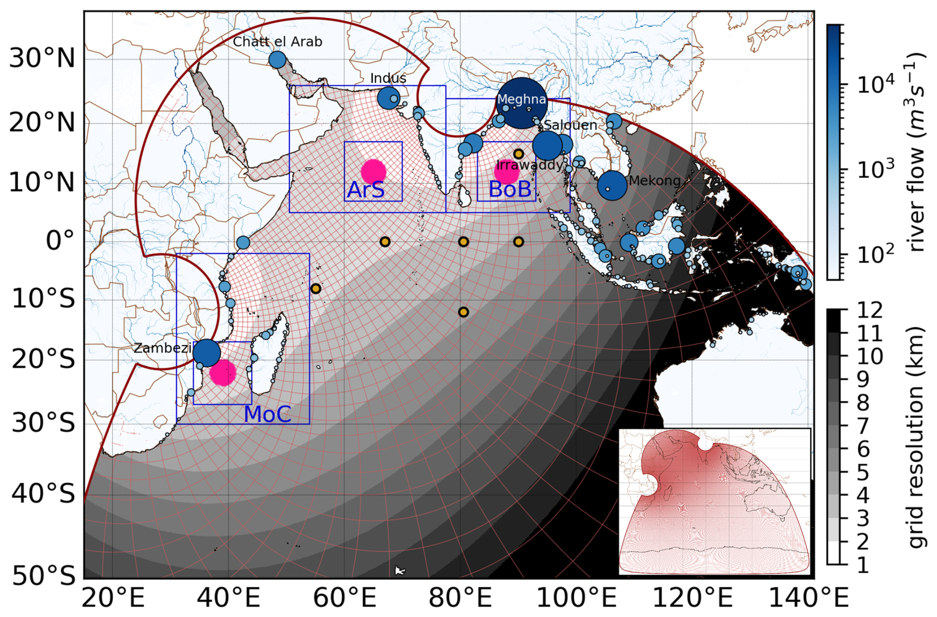
Figure 1 Model telescopic grid resolution (in km, gray scale), displaying every 50 gridlines (red lines). The south boundary reaches Antarctica with a maximum mesh size of 23 km. Blue shaded color-bar and dots show the 336 daily freshwater discharges simulated in the configuration (the size of the dots is proportional to their mean annual discharge over the period 2016–2021). The names of the domain's largest rivers are displayed on the map. Blue boxes in the best-resolved regions (ArS: Arabian Sea, BoB: Bay of Bengal, MoC: Mozambique Channel) are used to calculate spatial averages of temperature, salinity, sea elevation, energy spectra and Lagrangian trajectories (larger boxes for Fig. 6 and Table 2; smaller boxes for Figs. 2, 7, 9 and 10). The six yellow dots show the RAMA buoy locations for comparisons with in situ profiles (Fig. A2). The three pink circles show the particle release locations for the Lagrangian sensitivity analysis.

The lower resolution configuration (IndOc.12) uses the same features as IndOc.HR, except for its horizontal discretization, which is regular at $\mathrm{1}/\mathrm{12}$°.

Three regions of interest with contrasting ocean dynamics, corresponding to the best-resolved areas of the IndOc.HR coastal domain, are particularly analyzed in this study: the Arabian Sea (hereafter referred to as ArS), the Bay of Bengal (hereafter referred to as BoB) and the Mozambique Channel (hereafter referred to as MoC). These regions are used to calculate spatial averages of temperature, salinity, sea level and energy for the evaluation of the simulations (larger blue boxes on Fig. 1 used for Fig. 6 and smaller blue boxes on Fig. 1 used for Figs. 7 and 9).

2.1.3 Atmospheric and open ocean boundary conditions

Atmospheric forcing on the free surface boundary is calculated from the bulk formulae of Large and Yeager (2004), using wind stress, pressure, solar/thermal radiations, humidity and temperature provided by the ECMWF's ERA5 daily mean product at 0.25°. Open lateral boundary conditions and initial state for currents, temperature, salinity and sea surface elevation are provided by the daily mean CMEMS GLORYS12V1 product at $\mathrm{1}/\mathrm{12}$° (Lellouche et al., 2021). A temporal nudging layer is configured in regions where the resolution of the telescopic grid is coarser than that of the $\mathrm{1}/\mathrm{12}$° GLORYS forcing. This only occurs is the southeastern part of the domain, south of 50° S and around Australia, as shown by the grid resolution in Fig. 1. In these areas, temperature and salinity fields are relaxed toward their better-resolved GLORYS counterpart, over the full water column, using a relaxation time scale that decreases smoothly with the difference in resolution between the two grids. Relaxation is therefore greater at the southeastern edge of the domain, with a minimum time scale of 30 d. This nudging does not impact the three regions selected for model evaluation (ArS, BoB, MoC), ensuring that it does not artificially improve the agreement with observations in these areas. Tidal forcing is prescribed from the FES2014 global tidal model (Lyard et al., 2021), taking into account 9 barotropic components in phase and amplitude according to Pairaud et al. (2008, 2010).

2.1.4 Rivers

Our domain includes 336 rivers with a mean annual discharge >100 m³ s⁻¹ (Fig. 1), for a total annual discharge into the domain around 9400 km³ yr⁻¹ (averaged over 2016–2021). Those discharges are extracted from the gridded CMEMS Global Flood Awareness System (GloFAS-v3.1; Zsoter et al., 2021) forecasts characterized by unprecedented temporal (daily) and spatial (0.1°) resolutions. It combines satellite data, models (ECMWF and LISFLOOD) and in situ measurements. We identify river mouths locations by reconstructing the watercourses down to the coastal river outlets where water flows are at their maximum. When a river mouth corresponds to a delta, we ignore the different branches of the delta and simulate a single inflow point with a discharge corresponding to the sum of all the streams (as for the Ganges-Brahmaputra Delta for example). Among the 336 extracted rivers, 4 rivers have a mean annual discharge > 10 000 m³ s⁻¹ (Ganges-Brahmaputra-Meghna, Irrawaddy, Mekong, Zambezi), 11 rivers >5000 m³ s⁻¹ (Indus, Salouen, Godavari, Kapuas, Chatt el Arab, Pulau, Mahakam), 40 rivers >1000 m³ s⁻¹ and 92 rivers >500 m³ s⁻¹.

Each river daily inflow is introduced at the grid point closest to the river mouth, using a hybrid Neumann/Dirichlet boundary condition constrained to respect an imposed total flow, described by Nguyen-Duy et al. (2021).

2.1.5 Current-wave interaction

In consideration of the recommendations put forth by van Sebille et al. (2020) concerning the impact of waves on transport, at the large scales and relatively low grid resolutions considered here, the model incorporates a simplified parametrization for the influence of waves on currents, retaining only the dominant terms in the right-hand sides of the momentum Eqs. (2) and (3) below, i.e., the Stokes-Coriolis force (van Sebille et al., 2020; Jordà et al., 2007; Xu and Bowen, 1994). Besides, readers' attention is drawn to the fact that a similar but more precise parameterization with more terms is provided by Couvelard et al. (2020).

Here, the parametrization consists in an online one-way forcing utilizing the three-component Stokes drift vector $({\stackrel{\mathrm{̃}}{u}}^{\mathrm{s}},{\stackrel{\mathrm{̃}}{v}}^{\mathrm{s}},{\stackrel{\mathrm{̃}}{w}}^{\mathrm{s}})$ in m s⁻¹, extrapolated below the surface using the peak period, sourced in our study from the global CMEMS WAVERYS 0.2° product (CMEMS, 2019). The general wave-current equations of the SYMPHONIE model distinguish between the components ($u,v,w$) of the Eulerian current and the components (${\stackrel{\mathrm{̃}}{u}}^{\mathrm{s}},{\stackrel{\mathrm{̃}}{v}}^{\mathrm{s}},{\stackrel{\mathrm{̃}}{w}}^{\mathrm{s}}$) of the Stokes drift. The Stokes drift enters the Eulerian equations through the advection operator. The material derivative used in Eqs. (2) to (5) below includes the advection by the Lagrangian velocity $(u+{\stackrel{\mathrm{̃}}{u}}^{\mathrm{s}},v+{\stackrel{\mathrm{̃}}{v}}^{\mathrm{s}},w+{\stackrel{\mathrm{̃}}{w}}^{\mathrm{s}})$, i.e. Eulerian current + Stokes drift, such as:

$$\begin{array}{}\text{(1)}& \begin{array}{rl}{D}_t.=& {\partial }_t.+{\partial }_x\left[\left(u+{\stackrel{\mathrm{̃}}{u}}^{\mathrm{s}}\right).\right]+{\partial }_y\left[\left(v+{\stackrel{\mathrm{̃}}{v}}^{\mathrm{s}}\right).\right]\\ & +{\partial }_z\left[\left(w+{\stackrel{\mathrm{̃}}{w}}^{\mathrm{s}}\right).\right]\end{array}\end{array}$$

The horizontal components of the Eulerian current are given by:

$$\begin{array}{}\text{(2)}& {\displaystyle }{D}_{t}u=+f\left(v+{\stackrel{\mathrm{̃}}{v}}^{\mathrm{s}}\right)-{\displaystyle \frac{\mathrm{1}}{{\mathit{\rho }}_{\mathrm{0}}}}{\displaystyle \frac{\partial p}{\partial x}}+{\displaystyle \frac{\partial }{\partial z}}\left(K_m{\displaystyle \frac{\partial u}{\partial z}}\right)+{\mathrm{\Delta }}^{\mathrm{2}}u\text{(3)}& {\displaystyle }{D}_{t}v=-f\left(u+{\stackrel{\mathrm{̃}}{u}}^{\mathrm{s}}\right)-{\displaystyle \frac{\mathrm{1}}{{\mathit{\rho }}_{\mathrm{0}}}}{\displaystyle \frac{\partial p}{\partial y}}+{\displaystyle \frac{\partial }{\partial z}}\left(K_m{\displaystyle \frac{\partial v}{\partial z}}\right)+{\mathrm{\Delta }}^{\mathrm{2}}v\end{array}$$

where f is the Coriolis parameter, ρ₀ is the reference seawater density, p is the pressure, and Δ² is a horizontal bilaplacian operator. Then, the equations for temperature T and salinity S are defined such as:

$$\begin{array}{}\text{(4)}& {\displaystyle }{D}_{t}T={\displaystyle \frac{\partial }{\partial z}}{K}_h{\displaystyle \frac{\partial T}{\partial z}}+\mathrm{\Delta }T+{\displaystyle \frac{\partial }{\partial z}}I\text{(5)}& {\displaystyle }{D}_{t}S={\displaystyle \frac{\partial }{\partial z}}{K}_h{\displaystyle \frac{\partial S}{\partial z}}+\mathrm{\Delta }S\end{array}$$

with K_m and K_h the vertical turbulent viscosity and diffusivity coefficients for momentum and tracers, calculated by the turbulent closure scheme (k-ϵ), I the radiative forcing term and Δ a horizontal diffusion operator.

The sea surface height η is given by:

$$\begin{array}{}\text{(6)}& {\partial }_t\mathit{\eta }=-{\partial }_x\underset{-h}{\overset{\mathit{\eta }}{\int }}(u+{\stackrel{\mathrm{̃}}{u}}^{\mathrm{s}})\mathrm{d}z-{\partial }_y\underset{-h}{\overset{\mathit{\eta }}{\int }}(v+{\stackrel{\mathrm{̃}}{v}}^{\mathrm{s}})\mathrm{d}z+P-E\end{array}$$

where P−E is the precipitation and evaporation budget. The continuity equation is applied to the Lagrangian velocity, defined as the sum of the Eulerian current and the Stokes drift, to deduce its vertical component, as follow:

$$\begin{array}{}\text{(7)}& {\partial }_x\left(u+{\stackrel{\mathrm{̃}}{u}}^{\mathrm{s}}\right)+{\partial }_y\left(v+{\stackrel{\mathrm{̃}}{v}}^{\mathrm{s}}\right)+{\partial }_z\left(w+{\stackrel{\mathrm{̃}}{w}}^{\mathrm{s}}\right)=\mathrm{0}\end{array}$$

Eulerian tracers T and S are therefore both displaced consistently by the Lagrangian velocity, ensuring coherence between Eulerian and Lagrangian transport formulations.

2.2 The simulations

2.2.1 Ocean simulations

Using the configuration and grid described above, we produced two twin simulations: a reference simulation, called IndOc.HR in the following and not including wave effects; and its twin simulation, called IndOc.HR-Sto in the following, including the effect of waves on Eulerian currents via the Stokes–Coriolis term in the momentum equations and via the explicit advection by Stokes drift (see Sect. 2.1.5). To estimate the potential added-value of the telescopic grid, we also produced a simulation called IndOc.12 in the following, using the same forcings and settings as IndOc.HR, but on a regular horizontal grid covering the same domain at $\mathrm{1}/\mathrm{12}$° resolution. Those three simulations are performed over the year 2017 after a two months spin up. Except for the wave effect, they are all subjected to the same forcings. The simulations are performed with a calculation time step of 200 s. Daily average outputs are stored, including current velocities, temperature, salinity, sea surface height and turbulent kinetic energy.

2.2.2 Lagrangian simulations

Three Lagrangian numerical experiments are performed offline using the SYMPHONIE Lagrangian tool (as described in Weiss et al., 2024b), each using the daily 3D velocity fields produced by the three simulations IndOc.HR, IndOc.HR-Sto and IndOc.12 (Sect. 2.2). The particle advection is based on a Runge-Kutta second order advection scheme with an integration time step of the particle trajectories of 10 min. The current velocities are interpolated linearly in space (3D) and time at each particle position. The time derivative of the 3D position vector $X\left(t\right)=(x,y,z)\left(t\right)$ is equal to the stored Lagrangian velocities provided by each hydrodynamic simulation.

• In the classical case (IndOc.HR and IndOc.12), the Lagrangian velocity corresponds to the resolved Eulerian currents $(u,v,w)$ only:

  $$\begin{array}{}\text{(8)}& {\displaystyle \frac{\mathrm{d}X\left(t\right)}{\mathrm{d}t}}=\left\{\begin{array}{l}\frac{\mathrm{d}x\left(t\right)}{\mathrm{d}t}=u\left(t\right)\\ \frac{\mathrm{d}y\left(t\right)}{\mathrm{d}t}=v\left(t\right)\\ \frac{\mathrm{d}z\left(t\right)}{\mathrm{d}t}=w\left(t\right)+w_{\mathrm{t}}\left(t\right)+w_{\mathrm{s}}\left(t\right)\end{array}\right.\end{array}$$

• In the wave-modified case (IndOc.HR-Sto), the Lagrangian velocity includes the Eulerian currents $(u,v,w)$ dynamically modified by the Stokes-Coriolis force and the Stokes drift $({\stackrel{\mathrm{̃}}{u}}^{\mathrm{s}},{\stackrel{\mathrm{̃}}{v}}^{\mathrm{s}},{\stackrel{\mathrm{̃}}{w}}^{\mathrm{s}})$ as shown in Sect. 2.1.5, such as:

  $$\begin{array}{}\text{(9)}& {\displaystyle \frac{\mathrm{d}X\left(t\right)}{\mathrm{d}t}}=\left\{\begin{array}{l}\frac{\mathrm{d}x\left(t\right)}{\mathrm{d}t}=u\left(t\right)+{\stackrel{\mathrm{̃}}{u}}^{\mathrm{s}}\left(t\right)\\ \frac{\mathrm{d}y\left(t\right)}{\mathrm{d}t}=v\left(t\right)+{\stackrel{\mathrm{̃}}{v}}^{\mathrm{s}}\left(t\right)\\ \frac{\mathrm{d}z\left(t\right)}{\mathrm{d}t}=w\left(t\right)+{\stackrel{\mathrm{̃}}{w}}^{\mathrm{s}}\left(t\right)+w_{\mathrm{t}}\left(t\right)+w_{\mathrm{s}}\left(t\right)\end{array}\right.\end{array}$$

In all cases (Eqs. 8 and 9), the vertical displacement of the particles considers (i) a vertical turbulent random-walk diffusion term w_t based on the turbulent kinetic energy in the particle grid cell and a random number (Guizien et al., 2012), and (ii) a specific vertical velocity term w_s reflecting the particle buoyancy (Weiss et al., 2024b). Only buoyant particles are considered here (illustrated Sect. 5) with a rising velocity w_s=1 mm s⁻¹, oriented toward the sea surface. This value is within the lower range reported in the literature for specific plastic debris types such as light fibers, weathered or biofouled items (Waldschläger et al., 2020; Fischer et al., 2022; Kuizenga et al., 2022). It was chosen as an intermediate order of magnitude of average vertical velocities of surface currents, allowing such buoyant particles to be influences by vertical mixing processes in the surface layer rather than remaining strictly at the surface.

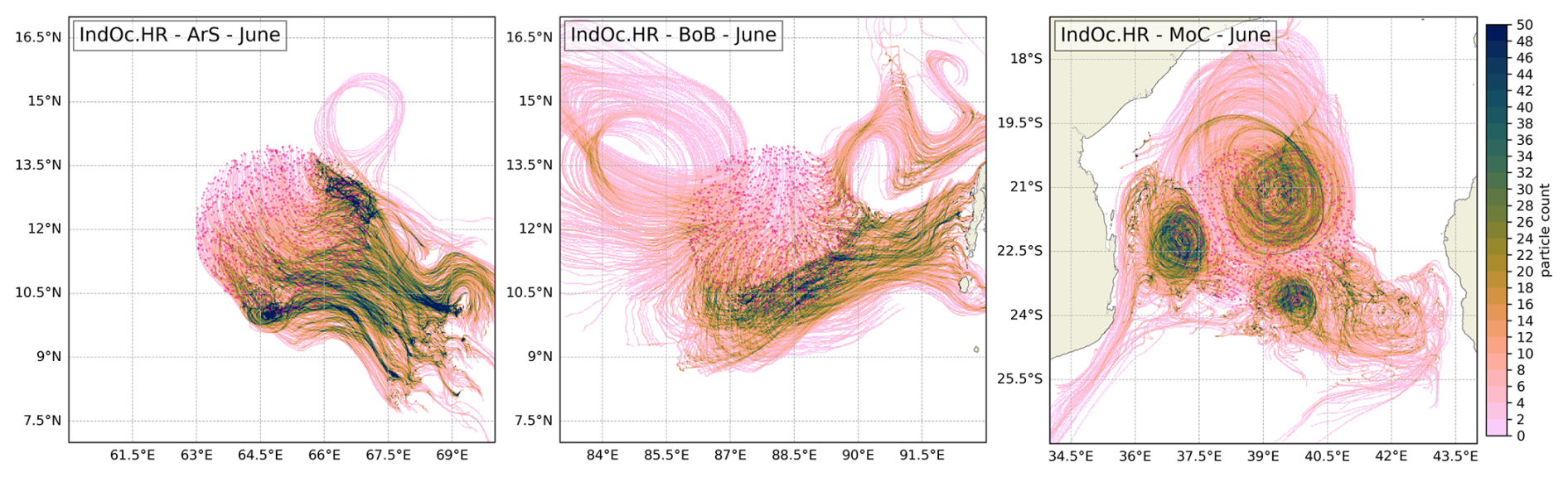
Figure 2 Illustration of the emission and dispersion of the buoyant particle plumes in June 2017 in the three studied regions, ArS, BoB and MoC, in the IndOc.HR simulation. The initial positions are shown as pink dots and color shades show the particle count in 2 km grid cells, highlighting the 30 d trajectories. A regional view of particle release locations is shown in Fig. 1.

Each Lagrangian experiment consists in releasing buoyant particles within each of the three high-resolution zones analyzed in this study, i.e. ArS, BoB and MoC. In each zone, particles are randomly released at the sea surface, between −1 and −2 m depth, within a circular emission area of 2° radius centered on the predefined central point of the zone (see Fig. 2). It results in three distinct emission regions, one per zone, for each experiment. One particle is released per minute on the first day of each month, followed by a 30 d drift period, resulting in 1440 trajectories per month per zone. Over a one-year period, a total of 51 840 particles are released in each Lagrangian experiment.

2.3 The observations

To evaluate the simulations, we use data-sets of Sea Surface Temperature (SST), Sea Surface Salinity (SSS), Sea Level Anomaly (SLA), temperature and salinity vertical profiles, and river discharges.

2.3.1 Satellite datasets

The CMEMS Level 4 Operational Sea Surface Temperature and Ice Analysis (OSTIA) product (CMEMS, 2015), providing daily gap-free maps at resolution 0.05° built from in situ (drifting and moored buoys) and remote infrared (multiple spatial sensors) observations, is used to evaluate the SST. The ESA Climate Change Initiative (CCI) weekly product at 0.5° resolution (Boutin et al., 2021) combining observations from the Soil Moisture and Ocean Salinity (SMOS) and Aquarius and Soil Moisture Active Passive (SMAP) spatial sensors is used to evaluate the SSS. Global satellite altimetry gridded Level 4 data from the CMEMS platform (CMEMS, 2021) at resolution 0.25° is used to evaluate the SLA. For comparison purposes, we remove from the simulated and observed daily SLA timeseries their temporal average over the period of comparison (2017) (see Eq. A1).

2.3.2 In situ data

In situ data from six buoys from the NOAA Research Moored Array for African-Asian-Australian Monsoon Analysis and Prediction (RAMA) project (McPhaden et al., 2009) are used to evaluate the SST and SSS. The CMEMS GLORYS12V1 reanalysis product (CMEMS, 2018), assimilates Argo in situ vertical profiles, with a large number of Argo floats continuously active during the year 2017 in the studied domain (around 700, leading to more than 25 000 profiles). This product is thus also used to evaluate the simulated temperature and salinity vertical profiles.

2.3.3 Hydrology datasets

The evaluation of rivers discharge is performed thanks to two global hydrology datasets. First, the HydroSHEDS atlas, at 15 arcsec resolution, i.e. $\mathrm{1}/\mathrm{240}$° or ∼ 0.5 km at the equator (Linke et al., 2019, long-term average over 1971-2000), is used to evaluate annual mean discharges and river catchment areas. Second, the Dai & Trenberth (D&T) climatology (Dai, 2017, based on scattered measurements between 1900 and 2018), is used to evaluate annual and monthly climatological mean discharges for the 47 individual rivers common to our domain and their dataset.

2.4 Analysis of river discharge

In this section, we examine the representation of rivers, comparing daily and annual discharges from GloFASv3.1 with HydroSHEDS, D&T climatology and the updated GloFASv4 datasets for some common rivers (Figs. 3, 4 and A4).

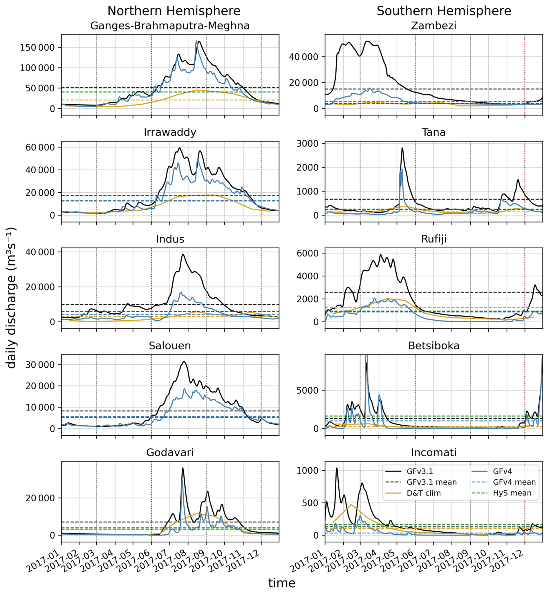
Figure 3 Daily discharges from GloFASv3.1 (model forcing, in black) and GloFASv4 (blue) for five major rivers in the Northern Hemisphere in Asia (Ganges-Brahmaputra-Meghna Delta, Irrawaddy, Indus, Salouen, Godavari) and in the Southern Hemisphere in East Africa (Zambezi, Tana, Rufiji, Betsiboka, Incomati) over the year 2017 (in m³ s⁻¹). The corresponding mean annual values calculated from GloFASv3.1, v4, and HydroSHEDS (green) are displayed with dashed lines and the D&T monthly climatology is in yellow.

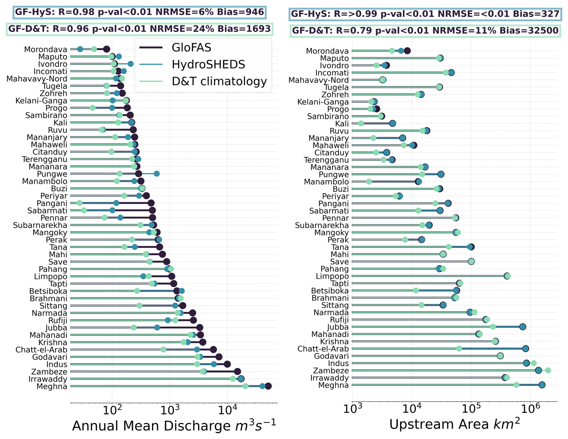
Figure 4 Comparison of annual mean discharges (left) and corresponding upstream catchment areas (right) for 47 rivers recorded in three datasets: the assimilated GloFASv3.1 model (GF, 0.1°), HydroSHEDS GIS (HyS, 15 arcsec, $\mathrm{1}/\mathrm{240}$°) and Dai & Trenberth climatology (D&T). Pearson correlation coefficients (R), NRMSE, and bias between GF and HyS and between GF and D&T are calculated from the 47 river mean values and shown in the headers.

The mean annual discharge of the 336 rivers considered in the IndOc domain (Indian Ocean and part of the South-East Asian seas) is estimated at 297 464 and 216 295 m³ s⁻¹ by GLOFASv3.1 and HydroSHEDS, respectively (i.e. +37 % in GLOFASv3.1). For the 47 rivers also listed in the D&T monthly climatology, the correlation coefficients between the three datasets over the year 2017 are nevertheless highly significant (> 0.96). The GLOFASv3.1 NRMSE calculated from the mean discharges of the 47 rivers is 6 % with a mean bias of 946 m³ s⁻¹ compared to HydroSHEDS, and 24 % with a mean bias of 1693 m³ s⁻¹ compared to D&T (Fig. 4). Most rivers with a mean annual discharge bias higher than 100 % are located on the East African coast, such as Jubba in Somalia, Pangani, Ruvu and Rufiji in Tanzania, Zambezi and Limpopo in Mozambique, Morondava in Madagascar, and Tana in Kenya (Southern Hemisphere in Fig. 3). On the contrary, rivers with a discharge bias smaller than 10 % are rather found in the BoB or in South-East Asia, such as the Irrawaddy in Myanmar, Subarnarekha, Brahmani, and Kali in India, Mahaweli in Sri Lanka, Perak, Terengganu, and Pahang in Malaysia (see Figs. 4 and A4).

These significant differences in mean discharge values cannot be attributed to errors in river catchment identification or boundary resolution. The total continental area of the 336 river catchments connected to the domain is indeed estimated to be equivalent, 13.247 and 13.168 million km² in GloFASv3.1 (0.1° res.) and in HydroSHEDS (0.5 km res.), respectively (i.e. a 0.6 % difference only). The correlation of river catchment areas between GloFASv3.1 and HydroSHEDS is > 0.99, with an NRMSE of < 0.01 % and an average bias of 327 km² among the 47 common rivers of Fig. 4. NRMSE and biases of river catchment areas compared to D&T are higher, since this climatology is based on measurement stations sometimes far upstream of river mouths (NRMSE = 11 % and bias = 32 500 km²). This also explains why GloFASv3.1 amplitudes in monthly mean discharges match poorly with D&T for some rivers like the Chatt-el-Arab, Manamblo or Betsiboka (Fig. A4).

This analysis thus reveals that the GloFASv3.1 version, used to prescribe river forcing in our simulations, tends to overestimate discharges, especially during peak flow periods (Fig. 3). The seasonality is however well represented. One of the explanations may be that GloFAS is forced by ERA5 atmospheric product, which tends to overestimate precipitation in the tropical zone (land and sea; Cucchi et al., 2020; Hassler and Lauer, 2021) with a tendency to show wet biases. Moreover, regional studies have observed systematic overestimation of river discharges, such as for the Ganges and Brahmaputra rivers (Hossain et al., 2023). This suggests that the structure of the hydrological model LISFLOOD on which the GloFAS-v3.1 product is based could also participate to the bias, by overestimating runoff from precipitation or underestimating evaporation from land and vegetation, which may vary between regions, depending on the disparity of the available observations used to calibrate the hydrological model (Alfieri et al., 2020). Those significant regional differences highlight the need for further investigations of hydrological processes in specific regions, such as East Africa or South Asia. Despite these biases, using GloFAS is an improvement in terms of river discharge representation, as it allows many more rivers to be included at a higher temporal resolution than traditional climatology. However, due to the overestimation observed in v3.1, our subsequent work has adopted the more recent GloFASv4, which will be used for upcoming multi-annual simulations to support future realistic Lagrangian scenarios based on river sources.

3 Evaluation of the simulations and circulation analysis

In this section, we first assess in Sect. 3.1 the ability of the IndOc.HR reference simulation to reproduce the spatial and temporal variability of ocean dynamics, including large and mesoscale hydrodynamics, through an analysis of the temperature, salinity and SLA. We then examine the difference related to the spatial resolution with IndOc.12 and the wave-induced effect through Stokes-Coriolis force and Stokes drift with IndOc.HR-Sto in Sect. 3.2. For model-observation comparisons through bias and correlation calculations, the SYMPHONIE model outputs are interpolated onto the corresponding observational product grids, i.e. SST to OSTIA (0.05°), SSS to CCI (0.5°), and SLA to CMEMS (0.25°).

The year 2017 used for comparison is characterized by relatively weak positive Indian Ocean Dipole anomaly (Zhang et al., 2018), no significant ENSO pattern (transition year from El Niño to La Niña, Kersalé et al., 2022), and few cyclonic systems during the cyclone season in the Southwest Indian Ocean, with only one notable system being ENAWO hitting northern Madagascar in March. In the following, the description of the circulation and the naming of currents is based on Schott and McCreary (2001) and Schott et al. (2009) with a schematic representation on Fig. A1.

3.1 The IndOc.HR reference simulation

3.1.1 Seasonal surface spatial patterns

The mean simulated and observed SST, SSS, and SLA are mapped (Fig. 5, IndOc.HR simulation), along with their corresponding biases, for the boreal winter (December, January, February – DJF) and summer (June, July, August – JJA). These two periods correspond partly to the Northeastern (NE) and Southwestern (SW) monsoon seasons, respectively.

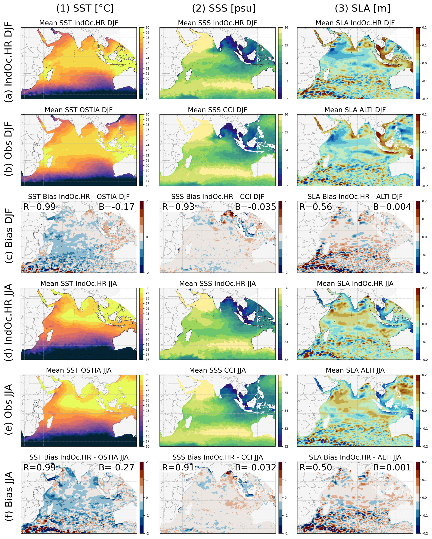
Figure 5 Spatial distribution of average SST (°C, column 1), SSS (psu, column 2) and SLA (m, column 3) over the boreal winter (DJF) and summer (JJA) of 2017: (a, d) in the IndOc.HR reference simulation and (b, e) in satellite observations, followed by (c, f) the average seasonal bias (model minus observations). The spatial Pearson correlation coefficient (R) and the average bias (B) are displayed over the maps.

At the basin scale, the simulated SST from IndOc.HR exhibits a significant spatial correlation with OSTIA observations (R=0.99 in DJF and JJA, Fig. 5 column 1). The simulation produces a cold SST bias on average, with a negative mean difference of −0.17 °C in DJF and −0.27 °C in JJA. Cold anomalies are mainly located to the east and north of Madagascar, encompassing the Northeast and Southeast Madagascar Current and the East African Coastal Current (see SST bias maps in Fig. 5-1c, -1f). During winter (DJF), the modeled SST fits perfectly with observations around the equator. This suggests an accurate representation of the cyclonic circulation between the Indonesian island of Sumatra to the east and the Somali Current to the west, that follows the Northeast Monsoon Current connecting the BoB to the ArS and the South Equatorial Counter-Current. Similarly, SST representation is good in the MoC and at the center of the BoB and ArS. On the other hand, warm (positive) biases are observed south of the MoC and north of the BoB (Fig. 5-1c). During summer (JJA), negative biases are more widespread, notably in the MoC, in the Andaman Sea (−0.5 to −1 °C) and north of the ArS. The South Java Current is also colder in summer in the simulation than in OSTIA. On the other hand, the Southern Gyre, the Great Whirl and associated upwelling wedges off the Somali coast tend to be warmer in the simulation, with a positive SST bias of around 0.4 °C. The mesoscale instabilities in the southern frontal zone, corresponding to the Retroflection of the Agulhas Current (around 40° S) and within the Supergyre (below 20° S), are simulated with temperature biases reaching −2 to 2 °C, attributable to the chaotic nature of ocean eddies, which cause strong spatial variability in their location.

The simulated SSS from IndOc.HR also shows a strong spatial correlation with the CCI observations for both seasons (R=0.93 in DJF and 0.91 in JJA, Fig. 5, column 2). There is a slight negative bias of −0.035 psu in DJF and −0.032 psu in JJA. Although the 0.5° resolution of the CCI product may not be sufficient to capture fine changes in coastal salinity, the model shows a tendency for river plumes to be fresher than the satellite observations. As suggested in the Sect. 2.4, these low salinity biases could be explained by the tendency of ERA5 to overestimate precipitation in the tropical zone (Cucchi et al., 2020; Hassler and Lauer, 2021, land and sea), which affects our simulations on two levels, firstly through the atmospheric forcing and secondly through the river forcing, as GloFAS is also forced by ERA5, overestimating river discharges. A second hypothesis is that the hydrological model used in GloFAS itself (LISFLOOD) could contribute to the biases by overestimating runoff from precipitation or underestimating evaporation from land and vegetation, which may vary between regions, depending on the disparity of the available observations used for calibration (Alfieri et al., 2020). This disparity is confirmed by the regional variability of the salinity bias. During both the NE monsoon (DJF) and the SW monsoon (JJA), the Gulf of Thailand and the Java Sea are fresher in the model compared to the CCI product (−0.5 to −2 psu). This is likely due to the influence of the Mekong freshwater plume to the north and to the flow of the Barito River to the south, the second main river of the Indonesian island of Borneo. Although the water in the Java Sea is fresher, this characteristic is not reflected in the Indian Ocean south of Java (with anomalies of 0 to +0.5 psu), strongly supplied by the Indonesian Throughflow (Zhang et al., 2022). Fresher biases are also observed off the Indus estuary NE of the ArS (especially in summer during the SW monsoon with −1 to −2 psu) and off the Zambezi River in the MoC (particularly during the austral summer (DJF) with the rainy season, i.e. −0.5 to −1 psu). On the contrary, the modeled BoB SSS is found to be saltier than the observations, with biases of up to +2 psu in the north, where the SSS is typically low around 31–32 psu. These significant differences could be linked to a poor representation of the circulation of the freshwater released by the Ganges-Brahmaputra-Meghna (GBM) delta in the extreme north of the BoB.

The spatial correlation between the simulated and observed SLA is lower than for SST and SSS, but remains statistically significant (at more than 99 % with p-values < 0.01), with R=0.58 in DJF and 0.47 in JJA (Fig. 5, column 3). No significant mean mean bias is observed (+0.001 to +0.005 m in both seasons). These lower SLA correlation values are mainly due to discrepancies in the mesoscale representation, particularly in the Southern Hemisphere, such as along the chaotic frontal zone of the Agulhas Current Retroflection, in the MoC and along the eddies of the Southeast Madagascar Current.

3.1.2 Regional surface annual cycles

Figure 6 shows the modeled and observed annual cycle of daily SST, SSS, and SLA in each regional subdomain (BoB, ArS and MoC). Table 2 evaluate the scores of the three simulations compared with the satellite observations, through the calculation of the correlation coefficient, the bias and the NRMSE.

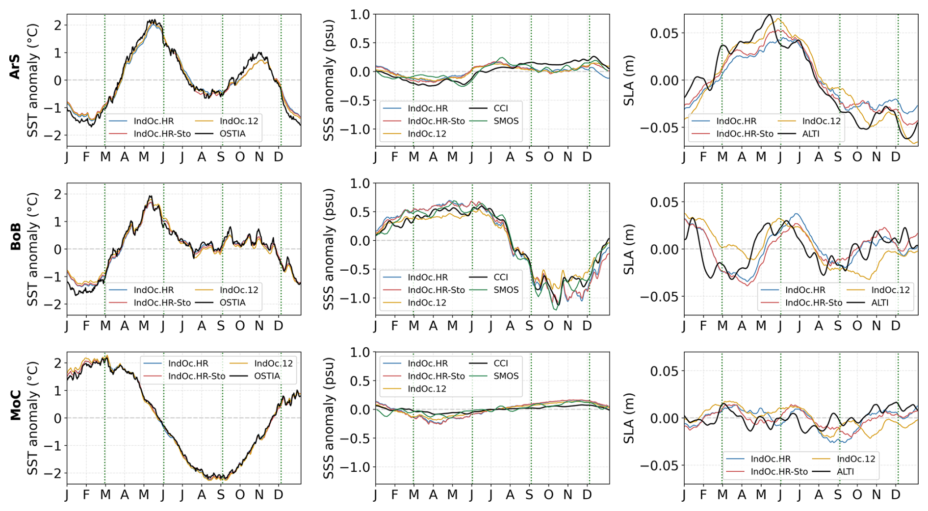
Figure 6 Time series of daily SST (°C, first column), SSS (psu, second column), SLA (m, third column) anomalies over 2017, spatially averaged over the three sub-regions (ArS, BoB and Moc, see Fig. 1). The observations are in black and the three modeled configuration in blue (IndOc.HR), red (IndOc.HR-Sto) and yellow (IndOc.12).

The correlation of IndOc.HR with OSTIA SST exceeds 0.99 in all regions, with NRMSE below 12 %. SST annual biases remain moderate, from −0.34 °C in BoB to −0.46 °C in MoC and −0.42 °C in ArS (Table 2). The fit is also consistent with in situ RAMA buoy data (Fig. A2), where similar cold biases are observed (ranging from −0.71 to −0.15 °C). These negative anomalies are known and reported in other regional studies (Trinh et al., 2024). It is related to cold biases in ECMWF-ERA5 atmospheric forcing, estimated by Yang et al. (2021) at −0.2 °C on average compared with OSTIA over a 15-year trend over the Indian Ocean (based on Fig. 10d of the reference study).

For SSS, the performance of IndOc.HR varies between basins. The temporal correlation with the CCI product reaches 0.98 in BoB and 0.95 in MoC, but is lower in ArS (R=0.68, Table 2). The highest NRMSE is found in the MoC (73 %), reflecting the strong variability in salinity along the African coasts, especially in the vicinity of the Zambezi River. Biases are generally negative compared to observations, with fresh biases down to −0.30 psu in BoB, −0.18 psu in ArS, and −0.09 psu in MoC. These fresh anomalies (down to −0.5 psu, Fig. 6) occur in SON for the ArS and BoB, and in MAM for the MoC, corresponding to periods following strong freshwater river discharges (starting in June in the Northern Hemisphere, and in December in the Southern Hemisphere, see Fig. 3). Spatially, the low salinity biases were mostly localized in the coastal zone near the mouths of the main rivers (i.e. Ganges-Brahmaputra-Meghna plume in the BoB and Indus in the ArS in JJA, Zambezi plume in the MoC in DJF, Fig. A3). It should be noted that CCI satellite data at 0.5° may not reliably represent the salinity of the coastal zone, it has indeed been shown that SSS from SMOS and SMAP satellites composing the CCI product have a good consistency in representing seasonal SSS variations, but tend to underestimate these variations substantially (Fournier and Lee, 2021), as it is the case in comparison with our simulation. Conversely, during the drier seasons, saltier anomalies (up to +0.3 psu) tend to appear in the model, notably in MAM for the ArS and BoB, and in SON for the MoC. Positive anomalies mainly occur offshore like in the BoB (Fig. 5).

The SLA temporal correlation for IndOc.HR is strongest in ArS (R=0.93), moderate in BoB (R=0.62), and low in MoC (R=0.34). The associated NRMSE values are 13 %, 25 %, and 35 % respectively (Table 2). SLA biases remain weak overall (ranging from −1.2 mm in MoC to +1.1 mm in BoB), although the relatively lower values in MoC may be due to the dominance of mesoscale and submesoscale dynamics in this region with high intrinsic variability and no seasonality observed in SLA variation (Fig. 6).

3.1.3 Regional vertical profiles

The IndOc.HR simulation accurately reproduces the properties of the water masses, as demonstrated by the good fit between the simulated vertical temperature and salinity profiles and the GLORYS assimilated products (Fig. 7). The stratification varies significantly between sub-regions.

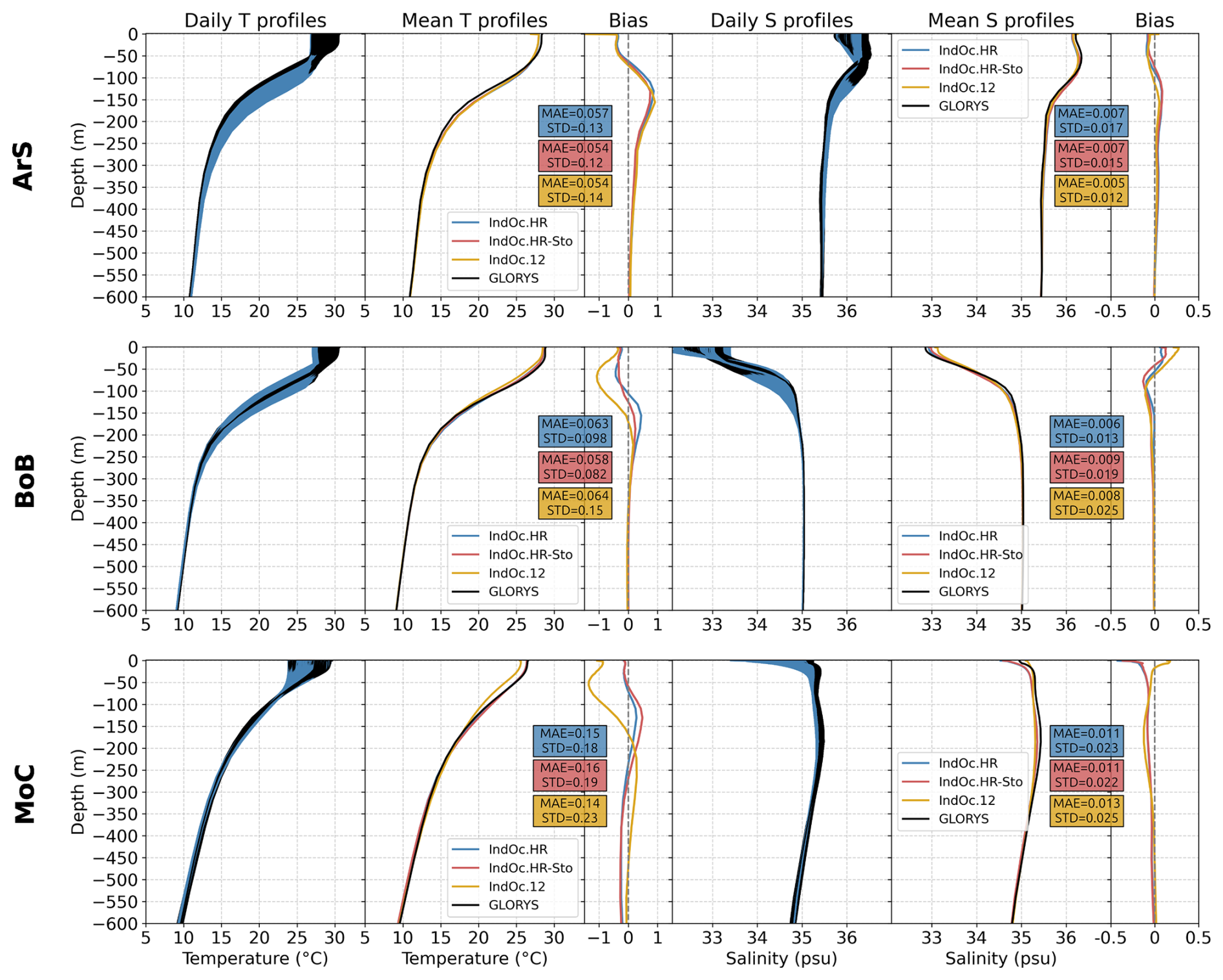
Figure 7 Temperature (°C) and Salinity (psu) vertical profiles averaged over the three sub-regions (ArS, BoB and MoC shown in Fig. 1) over 2017. All daily and mean profiles and biases (Eq. A4) spatially averaged, between the model outputs (in blue for IndOc.HR, red for IndOc.HR-Sto and yellow for IndOc.12) and the observations (in black) are represented. The Mean Absolute Error (MAE, Eq. A5) and the Standard Deviation (SD, Eq. A6) of the biases are shown.

In the ArS, the vertical profiles confirm the modeled slight cold (−0.36 °C) and fresh (−0.085 psu) bias in the surface layer (down to 70 m depth). Between 100 and 250 m depth, a warm bias appears between 0.5 and 1 °C, likely related to an overly deep thermocline. Despite theses biases, the mean absolute error (MAE) and the standard deviation (SD) in temperature remain low (0.057 and 0.13 °C, respectively). The salinity of the intermediate layer is better represented and the errors are minimal (MAE = 0.007 psu and SD = 0.017 psu).

In the BoB, the temperature profiles are similar, typical of tropical zones, but slightly colder at depth than in the ArS (with an average of 6.5 °C at 1000 m in the BoB instead of 8 °C in the ArS): the surface and intermediate waters of the ArS are denser than those of the BoB. The IndOc.HR simulation reproduces well the temperature and salinity characteristics in the surface layer (down to 30 m), although it has a slight cold (−0.26 °C) and salty bias (0.076 psu). Then, at the thermocline depths (between 30 and 150 m), the IndOc.HR simulation goes from a −0.4 cold to a 0.4 °C warm bias. The shallower halocline (between 20 and 100 m depth) goes from a salty to a fresh bias around 55 m depth. The MAE in temperature and salinity are equal to 0.063 °C and 0.006 psu, respectively, and the SD equal to 0.098 °C and 0.013 psu, respectively.

In the MoC, IndOc.HR exhibits weaker vertical gradients with less important river discharges (Fig. 1) than in the BoB. On average, surface water temperatures are colder (26.4 °C) than in the northern zones (28.0 °C in the ArS and 28.6 °C in the BoB), with a less pronounced thermocline. The IndOc.HR temperature profiles are quite close to the observations in the surface layer. Contrary to other regions, the temperature biases at depth (up to more than 1000 m) remain significant with ±0.2 °C (MAE = 0.15 °C and SD = 0.18 °C). The surface and intermediate waters of the IndOc.HR show a fresh bias compared to the observations (MAE = 0.011 psu and SD = 0.023 psu).

3.2 Sensitivity to spatial resolution and wave forcing

We now evaluate how the two sensitivity experiments, IndOc.HR-Sto (including wave forcing) and IndOc.12 (lower spatial resolution), differ from the reference simulation IndOc.HR.

3.2.1 Seasonal surface spatial patterns

The SST spatial correlation remains equally high in all three simulations (R=0.99 for both DJF and JJA), indicating robust large-scale pattern agreement with OSTIA in all configurations. The cold bias is slightly enhanced in the sensitivity simulations, with mean values of −0.22 to −0.35 °C (IndOc.HR-Sto) and −0.20 to −0.37 °C (IndOc.12), compared to −0.17 to −0.27 °C in IndOc.HR (Table 1, column 1). This indicates that both the inclusion of wave forcing and the coarser resolution tend to increase the negative SST bias, especially in JJA.

Table 1 Spatial Pearson correlation coefficient (Eq. A2) and seasonal spatial bias (Eq. A4) over the whole domain between the three annual simulations and the observations for SST, SSS and SLA. Associated p-values are all <0.01.

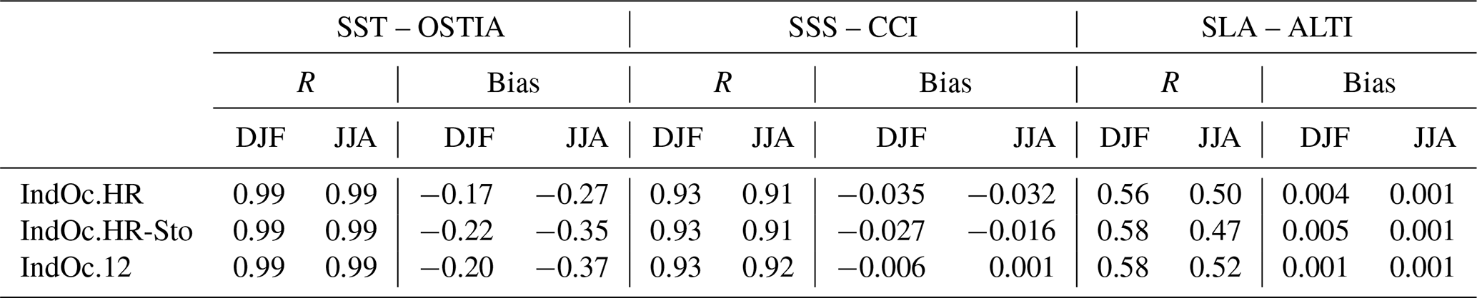
Table 2 Temporal Pearson correlation coefficient (Eq. A2), bias (Eq. A4) and NRMSE (Eq. A3 in %) between the three annual simulations and the observation datasets for SST, SSS and SLA averaged over the three sub-regions. All p-values are <0.01.

The SSS patterns are well captured in all simulations, with correlation coefficients ranging from R=0.91 to 0.93. Seasonal biases are slightly reduced in the sensitivity experiments, with negative mean biases of −0.027 to −0.016 psu in IndOc.HR-Sto and −0.006 to +0.001 psu in IndOc.12 (Table 1, column 2). These results indicate that both sensitivity configurations tend to simulate slightly saltier surface waters than IndOc.HR, especially in summer. The general patterns and freshwater plume locations remain consistent.

The SLA correlations are slightly lower than those for SST and SSS, due to the complexity of mesoscale dynamics and intrinsic variability, as well as the higher sensitivity of SLA to the location and structure of mesoscale features. The SLA discrepancy might be further amplified by the coarser resolution of the satellite-derived SLA product (0.25°) compared to the model resolution (2–9 km), which can lead to higher decorrelation when comparing fine scale dynamics. SST and SSS are generally less affected by such discrepancies due to their smoother spatial gradients. However, all correlations remain statistically significant (p < 0.01). The spatial correlation coefficients vary very little between the three simulations, ranging from R=0.47 in IndOc.HR-Sto in JJA to R=0.58 in IndOc.HR-Sto and IndOc.12 in DJF (Table 1, column 3). The mean SLA biases remain small in all simulations between +0.001 m in JJA and +0.005 m in DJF. Both sensitivity tests don't change the SLA correlations much, as the observations have a coarser resolution (0.25°) than our three simulations, and in particular don't capture the small scales represented by IndOc.HR and IndOc.HR-Sto.

3.2.2 Regional surface annual cycles

Compared to IndOc.HR, the IndOc.HR-Sto simulation shows similar performance in SST, with equally high correlation coefficients (R=0.99) and slightly increased cold biases: −0.49 °C in ArS, −0.39 °C in BoB, and −0.47 °C in MoC. NRMSE values remain close (10 %–13 %). For SSS, IndOc.HR-Sto shows a slight improvement in correlation in ArS (R=0.77 vs. 0.68) and BoB (R=0.98 unchanged), while maintaining a strong score in MoC (R=0.95). The fresh biases are slightly reduced in MoC (−0.08 psu vs. −0.09 psu), but unchanged in ArS (−0.18 psu). NRMSE decreases slightly in all regions (e.g., from 73 % to 71 % in MoC). SLA results improve slightly with the inclusion of wave forcing in ArS (R=0.95 vs. 0.93), and in MoC (R=0.41 vs. 0.34), and remain similar in BoB (R=0.60). The NRMSE also decreases slightly in MoC (28 % vs. 35 %). This suggests a small positive effect of wave forcing on SLA realism, particularly in regions dominated by mesoscale activity. This might be attributed to the Stokes-Coriolis force, which may modify the surface dynamics and current shear (McWilliams and Restrepo, 1999).

The IndOc.12 simulation shows slightly more different results. SST correlation remains high (R ≥ 0.98 in all regions), but biases are slightly stronger, especially in MoC (−0.62 °C) and BoB (−0.43 °C). NRMSE also increases in MoC (14 %), while remaining comparable elsewhere. For SSS, IndOc.12 shows lower NRMSE and bias than the HR configurations, particularly in BoB (NRMSE = 6 %, bias = −0.04 psu) and MoC (NRMSE = 33 %, bias < 0.01 psu). Temporal correlations also remain high (R > 0.94 everywhere). This result, although counterintuitive, may reflect a better consistency between the coarser CCI resolution (0.5°) and the smoother representation of coastal salinity gradients in our low resolution IndOc.12 simulation, rather than an improved physical realism. The SLA temporal fit in IndOc.12 decreases in BoB (R=0.36 vs. 0.60–0.62 in HR runs), and is close to zero in MoC ($R=-\mathrm{0.09}$). The SLA NRMSE is also the highest in all regions (33 % in BoB, 43 % in MoC), indicating that the coarser resolution degrades the representation of SLA variability, particularly in eddy-rich and dynamically complex zones.

3.2.3 Regional vertical profiles

In the ArS, both IndOc.12 and IndOc.HR-Sto simulate temperature profiles in line with IndOC.HR, with MAE values in the same range (0.054 °C) and low bias variability (SD = 0.12 to 0.14 °C). However, IndOc.12 shows a stronger cold bias (−0.47 °C) in the surface layer compared to HR (−0.36 °C). Salinity errors, already low in IndOc.HR (MAE = 0.007 psu), are slightly reduced in IndOc.12 (0.005 psu) with SD going from 0.017 in IndOc.HR to 0.015 in IndOc.HR-Sto and 0.012 psu in IndOc.12. The performance in all three simulations remains very close in this region.

In the BoB, where vertical stratification is more pronounced , more differences appear in temperature and salinity profiles. In the surface layer (down to 30 m), the cold bias is enhanced in IndOc.12 (−0.42 °C vs. −0.26 °C in HR) as well as the the salty bias (+0.24 psu vs. +0.076 psu in HR). Then, the thermocline bias transitions (between 30 and 150 m) observed in IndOc.HR (from cold to warm) is very attenuated in IndOc.HR-Sto, while IndOc.12 shows only a cold bias of −1 °C. Temperature MAE is slightly better in IndOc.HR-Sto (0.058 °C), and variability increases in IndOc.12 (SD = 0.15 °C), compared to IndOc.HR (0.098 °C) and HR-Sto (0.082 °C). For salinity, IndOc.12 is also slightly worse (MAE = 0.008 psu and SD = 0.025 psu) compared to IndOc.HR (MAE = 0.006 psu; SD = 0.013 psu).

In the MoC, where vertical gradients are weaker, the differences between IndOc.12 and both HR simulations are accentuated. IndOc.12 shows a −1.4 °C cold bias (at 55 m depth) while both HR simulations are quite close to the observations. The MAE in temperature are similar for the three simulation, while the SD in IndOc.12 is higher (0.23 °C vs. 0.18−0.19 °C in HR). For salinity, all simulations show small MAE (0.011–0.013 psu), but IndOc.12 again exhibits more variable biases (SD = 0.025 psu), compared to 0.022–0.023 psu in HR.

3.2.4 Synthesis of simulations performance

The comparison of spatial patterns and regional annual cycles reveals that no clear hierarchy can be establish regarding the quality of the three simulations performed: comparable correlation coefficients and error values (bias, NRMSE) for SSS and SST, in space and time (Tables 1 and 2) for IndOc.HR, .HR-Sto and IndOc.12. However, there are differences when considering the SLA and vertical profiles, revealing significant better performances for IndOc.HR and .HR-Sto.

The high-resolution configurations (IndOc.HR and IndOc.HR-Sto) perform better in representing SLA variability, particularly in mesoscale-active regions such as BoB and MoC. This is likely due to their finer representation of ocean dynamics, which is not captured by the lower resolution IndOc.12. However, SLA differences remain low due to the relatively coarse resolution of the compared observations (0.25°). Interestingly, IndOc.12 shows similar or even lower SSS errors in some regions, possibly benefiting from a resolution closer to that of the CCI product. However, IndOc.12 exhibits stronger biases and variability in vertical temperature and salinity profiles, particularly in BoB and MoC, reflecting a less accurate representation of stratification and subsurface structure. All three configurations reproduce key observed features, but HR simulations offer the most balanced performance, combining a good agreement with surface observations and vertical structures.

3.3 Seasonal variability of surface tracers and inferred dynamics

This section interprets the seasonal variability of SST and SSS, and the associated regional circulation patterns, which aligns with key dynamical features described by Schott et al. (2009), using the same current naming (see Fig. A1).

In the Northern Hemisphere, the SST peak in the ArS and BoB occurs in mid-May, with observed regional averages of 30.2 and 30.8 °C respectively (Fig. 6). Temperatures then decrease due to the summer monsoon-driven circulation reversal: cold waters from the Southern Hemisphere flow up into the ArS following the South Equatorial Current, the Northeast Madagascar Current and the East African Current. Significant upwelling wedges along the coasts of Somalia and Oman, associated with major eddies, i.e. the Southern Gyre, Great Whirl and Socotra Gyre, accentuate the surface cooling (well visible in the ArS in May–October, Fig. A3). The Southwest Monsoon Current connects the cooled waters from the ArS to the southern BoB and the Andaman Sea. During this season, strong precipitation and freshwater discharges also contribute to the cooling of surface waters in the BoB (Fig. 3), together with the strong vertical mixing caused by Southwest monsoon winds. The SST in those northern regions reaches an observed average summer minimum around 27.5 to 28.5 °C in August.

Starting in September, the second inter-monsoon season is characterized by the second circulation reversal to the south of India and a strong decrease in the intensity of the East African Current, as well as the Somalia and Oman upwellings (see the maps of mean kinetic energy (MKE, Eq. A7) in DJF in Fig. A5). As a result, the SST increases by 1.5 °C in the ArS and 0.5 °C in the BoB until November (Fig. 6). This period marks the sea surface winter cooling by the strong Northeast monsoon winds blowing to the North of the sub-basins (as shown in Figs. 5 and A3 during DJF and November–April). The regional SST reaches its minimum in February, around 26.3° in the ArS and 27.1° in the BoB.

In the Southern Hemisphere, the annual cycle of SST is reversed, and only two seasons are observed (unlike the four seasons in the North, Fig. 6). The hot and rainy season in the MoC (austral summer in November–April, Fig. A3) causes SST peaks in February-March, with observed mean regional SST at 29 °C. The cold and dry season (austral winter in May–October, Fig. A3) brings an abrupt drop in SST, with a mean regional minimum of around 24.5 °C in August.

In the Northern Hemisphere, the annual cycle of the SSS differs greatly between sub-basins: the mean SSS in the ArS is 3.7 psu higher than in the BoB (35.9 and 32.2 psu respectively) due to much lower freshwater inflows (Fig. 1) and higher evaporation. Moreover, the SSS variability in BoB has a higher amplitude. The summer monsoon, which starts in June (when the regional mean SSS is at its maximum of 32.9 psu), brings heavy rainfall to the continent, resulting in a rapid increase in river discharges to the BoB. The maximum discharge of around 160 000 m³ s⁻¹ in the Ganges-Brahmaputra-Meghna delta in Bangladesh occurs in mid-August (Fig. 3) and reduces the SSS by almost 2 psu in the sub-basin, with a minimum of 31 psu in mid-October. The decrease in river discharges to the north from September (Fig. 3), combined with the inversion of circulation from the SW summer monsoon to the NE winter monsoon, leads to a further increase in SSS in the BoB from December. This is due to the significant export of cold, low-salty water to the ArS in the south of India (Fig. A3), which induces its mean SSS drop of almost 0.3 psu (Fig. 6).

To the South, the annual variability of SSS in the MoC is low (0.4 psu) around an annual regional average of 35.1 psu. The SSS starts to decrease in December, which marks the beginning of the austral rainy season, reaching its minimum in April. This season is characterized by high river discharges in East Africa and Madagascar, the major river in the area being the Zambezi, with a GloFASv3.1 maximum discharge of around 50 000 m³ s⁻¹ (see Fig. 3). The austral dry winter (starting in May), is then characterized by a significant discharge reduction and thus a SSS increase in the coastal zone (Fig. 6).

4 Energy budgets analysis

The energy associated with ocean currents plays a critical role in the transport of marine debris, influencing their dispersion velocity, spread direction and resulting distribution. A detailed analysis of energy levels in circulation simulations is thus essential to understand and discuss the effect of simulated current fields on Lagrangian trajectories. Although Lagrangian kinetic energy (KE) computed along particle trajectories, would provide a more direct estimate of the energy experienced by marine debris, we focus here on Eulerian KE derived from the model gridded velocity field. This allows for a consistent comparison between simulations. In this section, we compare the energy budgets between our three simulations: IndOc.HR, .HR-Sto and .12.

4.1 Kinetic Energy budget

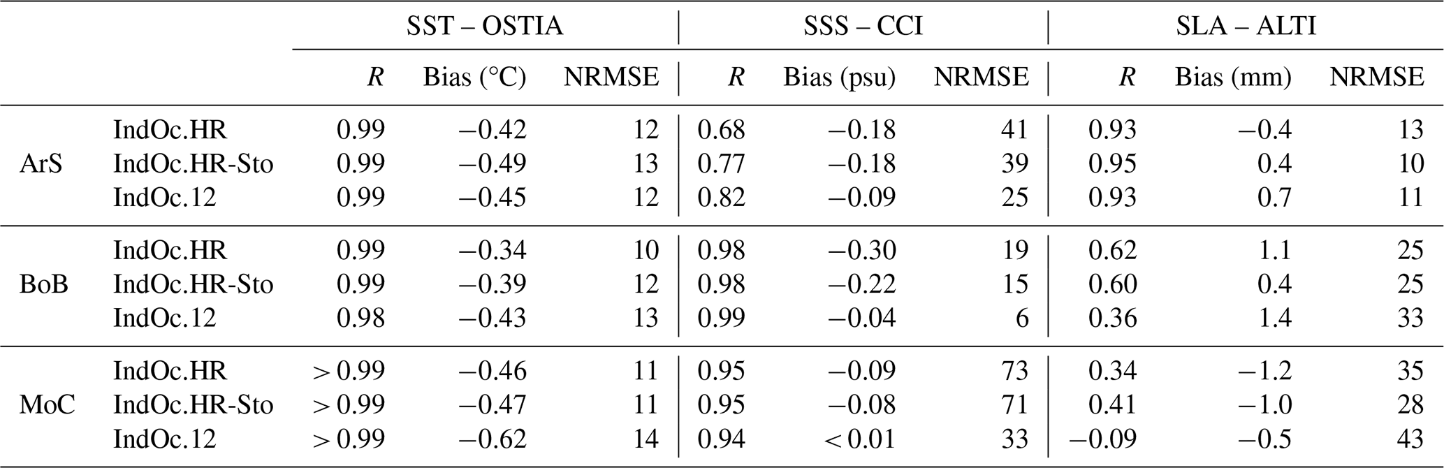
Figure 8 depicts the daily temporal evolution over 2017 (in addition to the two months of spin-up) of the KE averaged over the same IndOc domain for the three simulations conducted in this study (IndOc.HR, .HR-Sto and .12), for the surface (Fig. 8a) and over the whole depth (Fig. 8b). The energy in the 3D domain stabilizes over a two-months spin-up period (November to December 2016). The three simulations exhibit similar temporal variability at different time scales (daily to seasonal), but with varying levels of energy. The IndOc.HR-Sto configuration with wave forcing produces the most energetic simulation at the surface with an averaged KE of 62.88 m⁻² s⁻² (Fig. 8a), 8 % higher than IndOc.HR (Fig. 8c). In contrast, the IndOc.12 simulation has a significantly lower surface energy level than the two others with an averaged KE of 48.22 m⁻² s⁻² (Fig. 8a), 17 % smaller than in IndOc.HR, due to different scale and energy cascade representation (Fig. 8c). Although the differences are attenuated when integrating vertically, resulting in negligible differences on average over the depth and period (Fig. 8b, 6.59, 6.58 and 6.64 m⁻² s⁻² for IndOc.HR, IndOc.12 and IndOc.HR-Sto respectively), the low-resolution IndOc.12 simulation produces less energy during the most energetic periods (August to December), as expected.

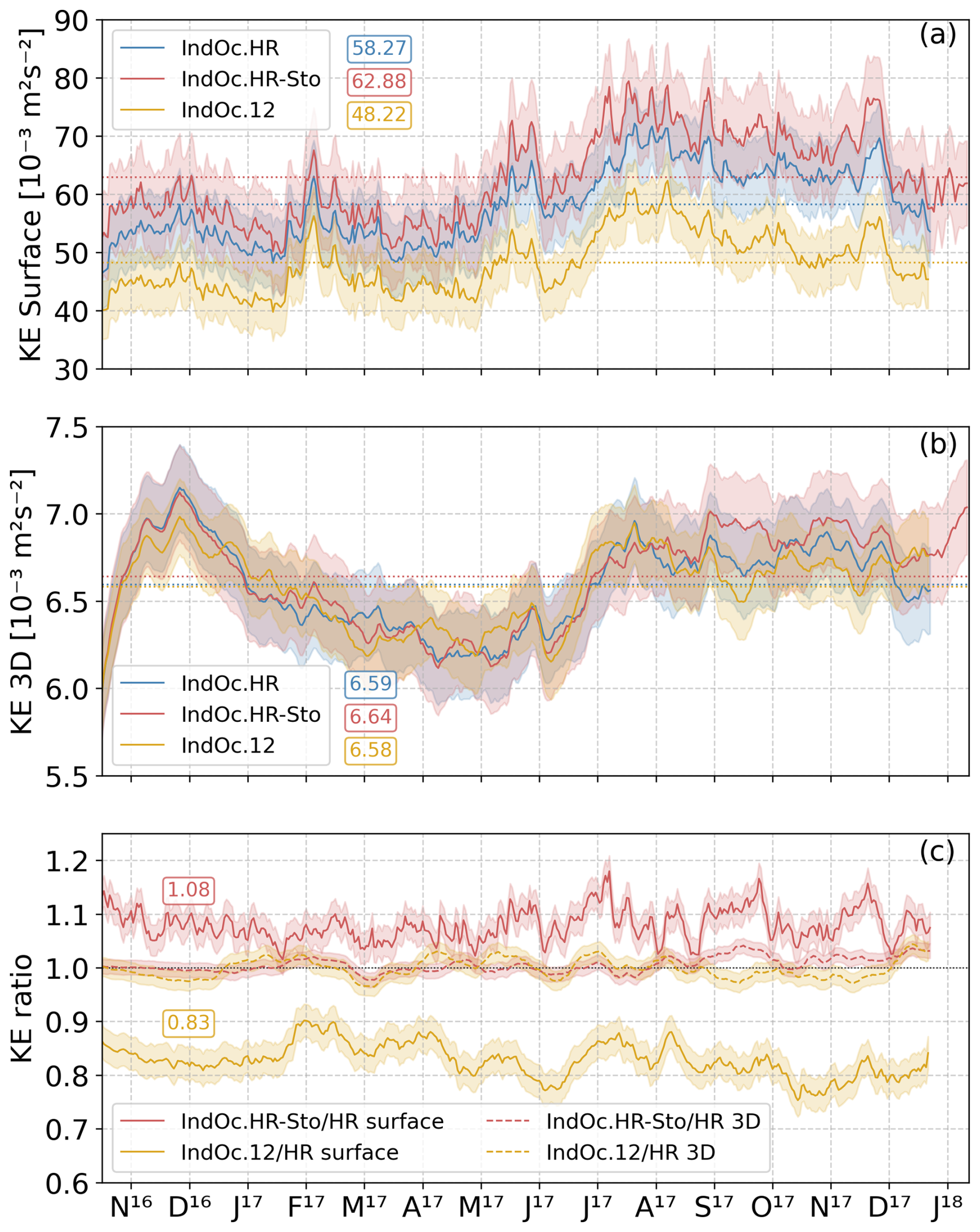
Figure 8 Time series of (a) the mean surface kinetic energy (KE in m⁻² s⁻²), (b) the mean 3D KE over the whole depth, and (c) the ratio of the mean KE of IndOc.HR-Sto (red) and IndOc.12 (yellow) simulations over IndOc.HR (blue) for the surface (solid lines) and the 3D (dashed lines). The three simulations are averaged over the same entire IndOc domain. The mean values over 2017 and the two-month spin-up are shown in the colored boxes (corresponding to the dotted lines).

4.2 Energy spectral density

The observed difference in energy amplitude between the HR simulations (1–3 km over the NW half domain) and the $\mathrm{1}/\mathrm{12}$° (≈ 9 km) simulation can be attributed to the representation of mesoscale (50–300 km) and submesoscale (< 50 km) activity (Herrmann et al., 2008; McWilliams, 2016; Waldman et al., 2017). To investigate dynamics spatial and temporal scales and eddy intensity across each region and grid resolutions, we examine their wavenumber-frequency power spectral density of KE as shown in Figs. 9, A6 and A7. For comparison purposes, the IndOc.HR, IndOc.HR-Sto and IndOc.12 daily average surface outputs were interpolated onto a $\mathrm{1}/\mathrm{50}$° (∼ 2 km) regular grid prior to spectral analysis. The wavenumber-frequency spectra (Figs. A6 and A7) are cut at the frequency of 2 d due to the daily time sampling of the outputs. Calculations are performed over the DJF and JJA seasons for the three studied regions (ArS, BoB, MoC). To complement, surface vorticity snapshots (Fig. 10) illustrate the distinct spatial dynamics resolved by the IndOc.HR and IndOc.12 simulations at meso and submesoscales.

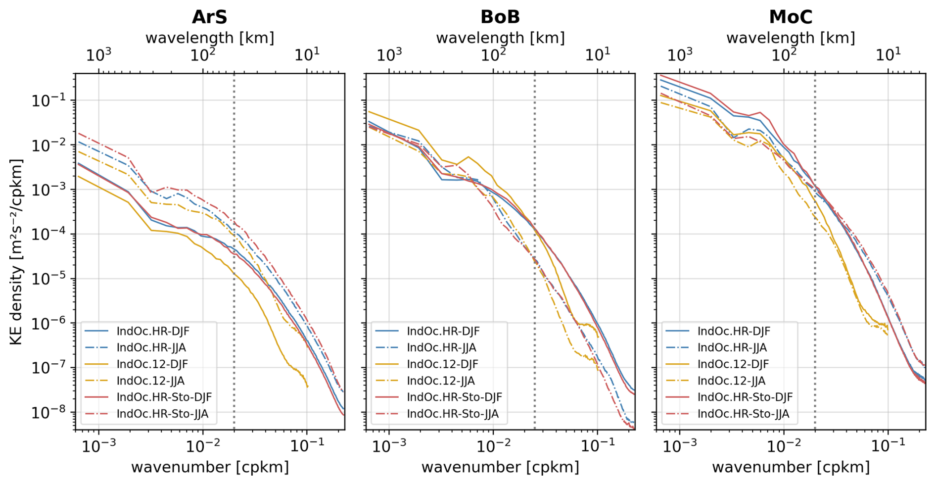
Figure 9 Wavenumber spectra of surface KE (m² s⁻²) for the IndOc.HR (blue), IndOc.12 (yellow) and Indoc.HR-Sto (red) simulations, over the DJF (solid lines) and JJA (dashed lines) seasons, for the three studied regions (ArS, BoB and MoC in Fig. 1).

Figure 10 Surface vorticity snapshots (s⁻¹) for IndOc.HR and IndOc.12 simulations on 1 January and 1 August 2017 over the three sub-regions (ArS, BoB and MoC, see blue boxes in Fig. 1).

The most energetic region is MoC, followed by BoB and then ArS (an order of magnitude separates the energy levels of MoC and ArS). This is supported by the vorticity snapshots in Fig. 10, where the MoC shows the largest and most intense mesoscale coherent eddies whatever the season. In general, the KE density is systematically higher in both HR simulations than in IndOc.12, for all regions and in every season, except for BoB during DJF where KE levels associated with large scale motions are higher in the IndOc.12 simulation (Fig. 9). Moreover, in every region and every season, there is a change in the KE spectral slopes as we move towards the small scales (below 50 km for ArS and MoC, below 40 km for BoB): the energy dissipates faster in the IndOc.12 simulation than in the IndOc.HR with more turbulence, and the energy gap between both resolutions increases. Vorticity snapshots on Fig. 10 show that sub-mesoscale structures such as small eddies and filaments are much more numerous and better represented in IndOc.HR than IndoC.12. The KE density spectra for IndOc.HR and IndOc.HR-Sto are quite similar in the three regions, but the IndOc.HR-Sto develops more energy than IndOc.HR during the JJA season in the ArS (at all scales) and during DJF in the MoC (at large scales), and less than IndOc.HR during JJA in the MoC (at large scales).

The disparities in terms of wavenumber-frequency spectra (Figs. A6 and A7) are highlighted in the high-frequency (< 10 d) and high-wavenumber (< 50 km) values that correspond to short-lived submesoscale balanced motions, but also in mesoscale motions (> 50 km). In the majority of 2D spectra, the energy peak is centered on structures with wavelengths of 100 to 200 km and periods of 10 to 30 d. These spectra show that a better representation of fine scales not only results in an increase in energy in the fine scales, but that it also leads to an inverse cascade of energy from the small to the large scales, also raising the energy levels of the large-scale structures with short and long periods (Gula et al., 2016; Klein et al., 2019). The exception of the BoB region, where the IndOc.12 simulation shows energy levels higher than IndOc.HR in winter (DJF), could be explained by the energy of the atmospheric forcings not dissipating towards the underdeveloped fine scales and therefore being concentrated in the large scales.

4.3 Scale representation and seasonality

For all regions, wavenumber spectra in Fig. 9 show that the energy differences between IndOc.12 and both HR simulations are greatest in winter (corresponding to DJF for ArS and BoB and JJA for MoC) and particularly in the motions scales below 100 km (through dissipation).

Figure 9 shows that the ArS exhibits the greatest seasonal differences in all simulations, with the summer season (JJA), corresponding to the southwest monsoon, generally more energetic than the winter season (DJF). In the western part of the sub-basin, baroclinic and barotropic instabilities are enhanced during this JJA period (Zhan et al., 2020), forming climatological mesoscale eddies such as the Great Whirl and the Socotra Eddy in the Somali Current region (see Fig. A1 and MKE, EKE maps on Fig. A5). Eddies are advected from the western formation zone towards the eastern part of the ArS (Trott et al., 2018), as shown by the EKE maps (Fig. A5). This west-to-east transport of energy is enhanced in the IndOc.HR simulation compared to IndOc.12. The JJA season in the ArS is also marked by maximum wind stress in the region (Fischer et al., 2002; Varna et al., 2023), leading to a stronger Stokes drift (Fig. A8), which in turn enhances the KE levels in IndOc.HR-Sto at this period.

In the BoB, seasonality is more visible for scale motions smaller than 100 km (Fig. 9), with more mesoscale and sub-mesoscale structures developed in winter (DJF), as shown on the vorticity snapshots (Fig. 10). However, we can see from the EKE (Fig. A5) that although the energy linked to eddies and sub-mesoscale is more homogeneous throughout the BoB in winter, it is in summer that the Southwest Monsoon Current, which bypasses Sri Lanka and runs up the west coast of the Gulf, is the strongest, associated with more intense mesoscale eddies. In the Northern Hemisphere, the temporal variability of the eddy field is thus partly related to instabilities resulting from changes in monsoon regimes and intraseasonal equatorial zonal winds (Cheng et al., 2018).

In the MoC, the differences between the seasons are the smallest, with large scales (> 50 km) slightly more energetic during DJF (warm rainy and cyclone season), whereas fine scales are slightly more energetic during JJA (cold dry season) in the IndOc.HR simulation. The MoC is part of the larger Agulhas Current system and is characterized by intense mesoscale eddy activity, dominated by large anticyclones (∼ 300 km) propagating southward, and occurring regularly over the year, as reported by Halo et al. (2014). These mesoscale structures are accurately reproduced by both IndOc.HR and IndOc.12 simulations, as illustrated by the surface vorticity snapshots (Fig. 10). However, only the IndOc.HR simulation represents the submesoscale structures and filaments along the coast and between the large eddies, which is more energetic during JJA (the austral winter).

4.4 Synthesis of energy levels and scale dynamics

The energy analysis highlights that the high-resolution simulation (IndOc.HR) more accurately captures both mesoscale and submesoscale dynamics compared to the lower resolution of IndOc.12 simulation, as expected. IndOc.HR exhibits higher KE levels at nearly all scales and in all regions, particularly in the 10–100 km range, where submesoscale processes are active. These fine-scale structures are associated with enhanced vorticity and filaments, especially along boundary currents and in energetic regions like the MoC. The IndOc.12 simulation dissipates energy more rapidly at small scales, failing to represent the full spectrum of eddy activity. This limitation leads to an underestimation of KE levels in both mesoscale and submesoscale ranges, with exceptions such as the BoB during DJF, where forcing energy accumulates at larger scales due to insufficient dissipation. The inclusion of the wave forcing in IndOc.HR-Sto through the Stokes-Coriolis force and Stokes drift leads to an increase in surface KE, particularly in regions and seasons of high wind stress (ArS during JJA, MoC during DJF), highlighting the role of wave-current interactions in energizing upper-ocean dynamics. Spectral results also indicate signs of an inverse cascade, an upscale transfer of energy from submesoscale to larger mesoscale structures, especially visible in the HR configurations. This finding aligns with previous theoretical and numerical work showing that submesoscale turbulence can energize larger scales through nonlinear interactions (Gula et al., 2016; Klein et al., 2019).

These differences emphasize the importance of resolving fine-scale dynamics for realistic ocean current simulations, with implications for tracer dispersion, vertical transport, and Lagrangian trajectory predictions.

5 Lagrangian trajectories

5.1 Trajectory statistics

The IndOc simulations are designed with the main objective of modeling the dispersion of marine debris in the Indian Ocean. In this final section, we present the effect of the three simulated current fields (IndOc.HR, IndOc.HR-Sto and IndOc.12) evaluated above on the representation of Lagrangian trajectories in the ocean surface layer. We simulate trajectories in our three regions with contrasting dynamics (ArS, BoB, MoC), and we take into account the temporal variability of the circulation through monthly releases of particles during a year (experiment described in Sect. 2.2.2 and illustrated in Fig. 2). Figure 11 shows the trajectory statistics obtained for each of the three simulations (IndOc.HR, IndOc.HR-Sto and IndOc.12), considering the plumes from the three regions (ArS, BoB, MoC) combined. Figure 12 shows these same trajectory statistics for each region separately. Finally, Fig. 13 shows trajectory roses with the main trajectory directions and distances traveled by the particles throughout the year for each region.

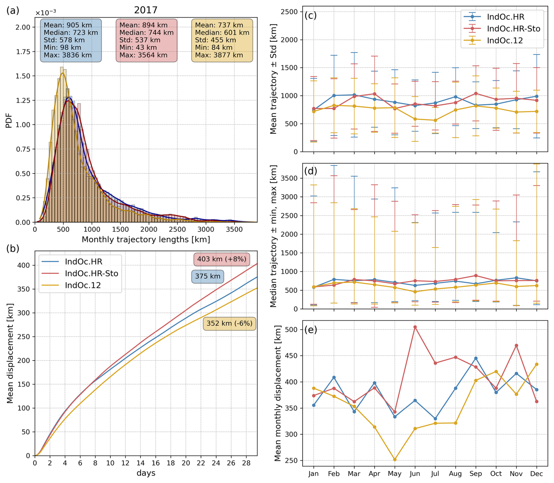
Figure 11 Statistical analysis of the Lagrangian trajectories obtained from the three ocean current simulations, i.e. IndOc.HR (blue), IndOc.HR-Sto (red) and IndOc.12 (yellow), considering the plumes from the three studied regions. (a) Histogram of monthly trajectory lengths, i.e. actual distances traveled. (b) Time evolution of the mean displacement of the plumes, i.e. the mean straight-line distance from the release position during the 30 d drift of each particle over 2017. (c) Monthly variability of the mean monthly trajectory length and (d) median monthly trajectory length with [min, max] distances traveled by the particles, and, (e) mean monthly displacement between the release position and the position after 30 d of drift (mean straight-line distance).

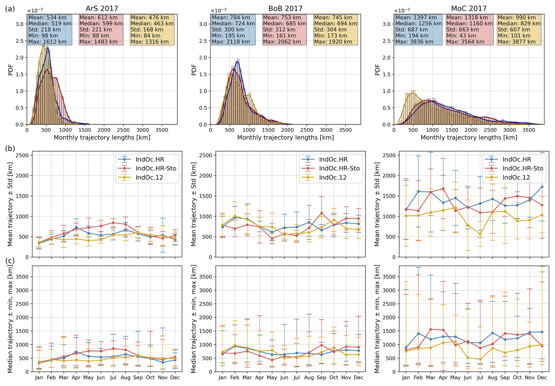
Figure 12 Statistical analysis of the Lagrangian trajectories for the three studied regions separately, i.e. ArS (column 1), BoB (column 2) and MoC (column 3), obtained from the three ocean current simulations of the study, i.e. IndoC.HR (blue), IndOc.HR-Sto (red) and IndOc.12 (yellow), (a) Histogram of the monthly trajectory lengths of the particles. (b) Monthly evolution of the mean ± SD, and (c) median trajectory lengths with [min, max] values, during 30 d over the year 2017.

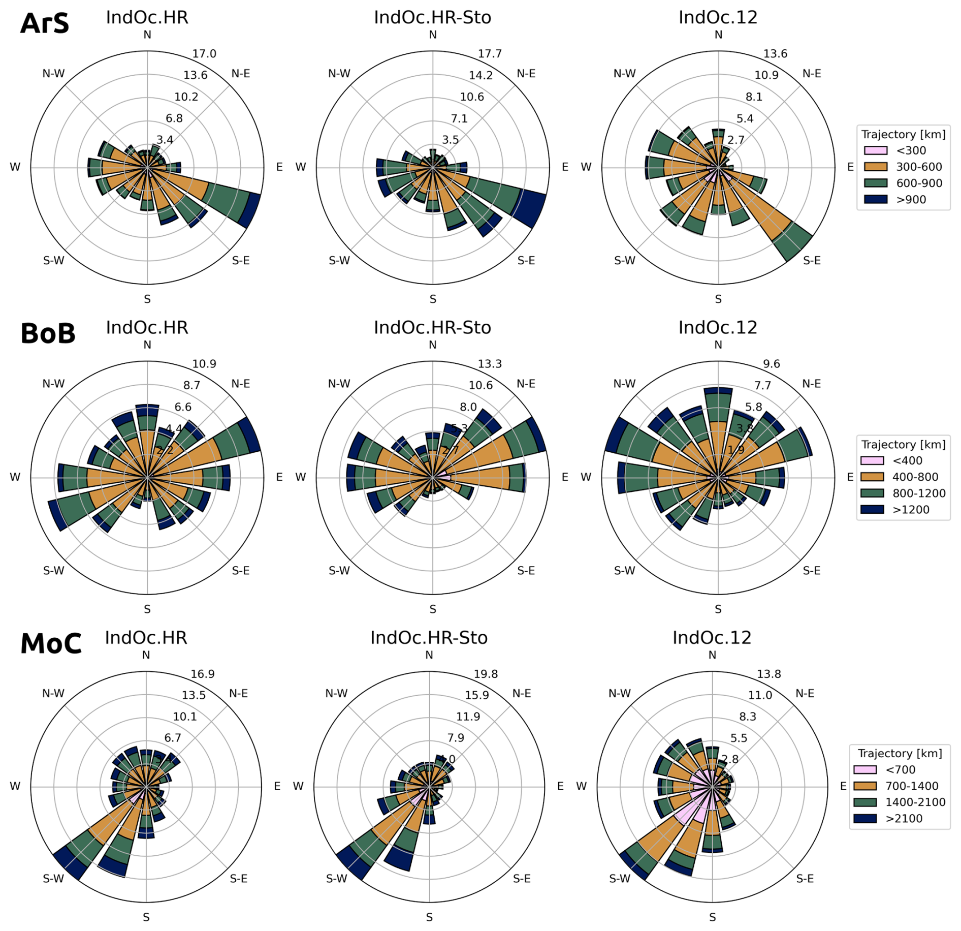
Figure 13 Annual trajectory roses for the three regions (ArS, BoB, MoC) for the three simulations (IndOc.HR, IndOC.HR-Sto, IndOC.12). The size of the arrows indicates the frequency of particles that follow the corresponding direction (%). The colors indicate the length of the particle 30 d trajectories in the corresponding direction.

Figure 11a shows that the PDF of trajectory lengths reaches a maximum 100–150 km smaller for particles released in IndOc.12 than in both HR simulations. The mean trajectory length in IndOc.12 (737 km) is 168 km shorter than in IndOc.HR (905 km) and 157 km shorter than in IndOc.HR-Sto (894 km). Similarly, the median trajectory length obtained from IndOc.12 is 122 km shorter than in IndOc.HR and 143 km shorter than in IndOc.HR-Sto. The spread of the trajectory length distribution is greater in the case of the HR simulations compared with IndOc.12, as shown by the standard deviation values (455 km in IndOc.12 vs. 578 and 537 km in IndOc.HR and IndOc.HR-Sto respectively). Figure 11b shows that the mean displacement of the particle plume is accentuated not only by the HR current fields but also by the Stokes drift. The particles end their 30 d trajectories on average 6 % closer to the release position in the IndOc.12 simulation than in IndOc.HR, and 8 % further away in the IndOc.HR-Sto simulation. The deviation between both HR simulations and IndOc.12 is visible from the second day of drift. The deviation between IndOc.HR and IndOc.HR-Sto is visible from the ninth day of drift. These deviations in trajectory lengths and plume displacements reflect the differences in KE levels generated at the ocean surface by the three different simulations (Fig. 8c): the higher KE in IndOc.HR and IndOc.HR-Sto enables stronger and more variable currents that enhance particle dispersion, while the lower KE in IndOc.12 results in slower and less dispersed trajectories. Looking at the monthly variability over the year (Fig. 11c, d, e), the statistical differences between the three simulations can vary over time, but the trajectories produced by both HR simulations are on average always longer (except in February but still very close) and more spread out (except in January, October and December but still very close) than those produced by the IndoOc.12 simulation.

5.2 Regional analysis

In order to evaluate the variability of these statistics, it is preferable to analyze the three regions separately in order to link the trajectories generated to the regional dynamic processes at play. Whatever the region, the average trajectory length of the particles in 30 d is always lower in IndOc.12, and the maximum of the PDF is reached on average for shorter trajectory lengths (Fig. 12). The distances traveled by the particles are much longer and the distribution of trajectories is wider in the MoC, followed by trajectories in the BoB and then in the ArS. This is consistent with the KE ratios reported in the spectra of Fig. 9, which show a MoC region that is much more energetic than BoB and ArS, with the presence of coherent mesoscale eddies of high intensity (Fig. 10). The most pronounced difference between the trajectories produced by both HR simulations and IndOc.12 also corresponds to the MoC region (Fig. 12a). This suggests that in highly dynamic regions with a strong geostrophic component, the resolution of the current fields is a critical factor for the study of Lagrangian dispersion in term of spread velocities and trajectory lengths.

In the ArS region, the trajectories from HR simulations are clearly longer than in IndOc.12 from March to August, then tend to be equivalent on average from September to February (Fig. 12b, c). The particle dispersion is accentuated in the IndOc.HR-Sto simulation that exhibits the most significant seasonal variability of trajectory statistics (which is consistent with the seasonal variation in KE spectra of Fig. 9, where JJA exhibits increased energy levels particularly at meso and submesoscales, enhancing particle dispersion during the monsoon season): mean and median trajectory lengths are almost 300 km greater in IndOc.HR-Sto current fields from March to August compared to IndOc.12 and from May to August compared to IndOc.HR. This annual variability corresponds to the monsoon cycle (observed for example in SLA curves in Fig. 6). From March to August (positive SLA in the ArS), the reversal of the circulation in the Northern Hemisphere is followed by the south-west summer monsoon (JJA). This is a period of maximum wind stress in the region (Fischer et al., 2002; Varna et al., 2023), producing the highest Stokes drift, as shown in Fig. A8, with a higher KE particularly in large and meso- scales and a more intense vorticity field than the rest of the year, as illustrated in Fig. 9 (JJA curves) and Fig. 10. This demonstrates the link between dispersion velocity and submesoscale representation associated with higher energy levels. It is interesting to note that during the south-west monsoon season, the prevailing direction of Lagrangian trajectories in the ArS is East-Southeast, following the total current direction (Fig. A9, JJA), while the Stokes drift points Northeast-East (Fig. A8, JJA). The trajectory roses demonstrate that the wave forcing can play a key role in shaping the buoyant particle drift, accentuating significantly the particle velocities and thus the trajectory lengths during strong wind periods. Throughout the year, particles move most frequently in an East-Southeast direction (Fig. 13, ArS), demonstrating the dominance of the southwest monsoon over the northeast monsoon in dispersion patterns.

In the BoB region, the closer energy levels between the three simulations (Fig. 9) is reflected by closer trajectory statistics (Fig. 12a). While KE associated with large to meso scales (> 60 km) in the IndOc.12 simulation is higher than both HR simulations in DJF, there is no clear differences in the average trajectory length. However, the fact that HR simulations still have more energy associated with fine scales (< 40 km) is sufficient to produce trajectory statistics on average longer than in IndOc.12 (Fig. 12a). The effect of the monsoonal circulation on trajectory statistics is not as marked as in the ArS (Fig. 12b, c). This is associated with much greater variability in particle trajectories in terms of direction and length (as shown by Fig. 13, BoB). No seasonality is indeed observed in energy levels associated with large scale (> 100 km) in the HR simulations, while accentuated energy levels are associated with small scales (< 100 km) during DJF compared to JJA (Fig. 9, BoB). During the summer monsoon (JJA), the prevailing direction of particle trajectories is Northeast-East (Fig. A10). The presence of Stokes drift in the IndOc.HR-Sto simulation does not accentuate the trajectory lengths, nor does it accentuate the energy densities to any great extent (Fig. 9, BoB). It is interesting to note that during this JJA period, there is more variability in trajectory directions in the IndOc.12 than in both HR simulations. This probably reflects the lack of coherent mesoscale structures in the lower resolution IndOc.12, resulting in more dispersed particle directions. In contrast, the HR simulations better resolve mesoscale features that guide particles along more consistent pathways, reducing directional variability.

In the MoC, a slight decrease in the trajectory lengths is visible from May to October, corresponding to the cold and dry season. The KE levels associated with large to meso- scales (> 40 km) are indeed lower in the JJA period than in the DJF period (Figs. 9, A6, A7). However, the dissipation through submesoscale (< 40 km) is enhanced during JJA compared with DJF. The difference in statistics between IndOc.HR-Sto and IndOc.HR is smaller in the MoC compared to the other two regions, indicating that the effect of waves is less significant here, both on the distances traveled (Fig. 12) and on the direction of the trajectories (Fig. A11). The Stokes drift in this region is southeast-to-north on average throughout the year with lower intensities than in the Northern Hemisphere (Fig. A8), contrasting with the predominant energy transfers of the oceanic circulation from northeast to southwest (Fig. A5). As a result, particles move most frequently in an East-Southeast direction (Fig. 13, MoC). Generally, in the IndOc.HR-Sto simulation, the particles tend to be channeled more in privileged directions, whereas in the IndOc.12 simulation the variability of the trajectories is accentuated in all directions (as in the other two regions, Fig. 13). The wave forcing effect may be negligible compared with the strong geostrophic component of ocean dynamics in this region.

5.3 Synthesis of resolution and wave forcing effects on particle dispersion

The IndOc.HR simulation, used as reference, produces longer and more dispersed Lagrangian trajectories than the lower resolution of IndOc.12, highlighting the crucial role of high-resolution current fields in capturing fine-scale structures that enhance dispersion. The differences in trajectory lengths and plume displacement are visible from the early stages of drift and are consistent with higher kinetic energy levels at the surface in IndOc.HR. Compared to IndOc.HR, the IndOc.HR-Sto simulation, which includes the wave effect through the Stokes-Coriolis force and Stokes drift, generates even more extended and anisotropic trajectories, especially during the monsoon season in the ArS, where wave-induced transport becomes significant. However, in regions dominated by geostrophic dynamics, such as the MoC, the Stokes drift contribution remains marginal. IndOc.HR offers a better representation of mesoscale and submesoscale variability than IndOc.12, while the implementation of wave forcing in IndOc.HR-Sto further improves Lagrangian transport under strong wind periods. These results confirm that both resolution and wave effects are key factors to accurately simulate surface drift in the Indian Ocean.

6 Conclusions

The goal of this study is to address current limitations in modeling the Indian Ocean circulation and its implications for marine debris dispersion in the region, by developing a new regional configuration with enhanced realism. Existing large-scale simulations of the Indian Ocean generally rely on horizontal resolutions of $\mathrm{1}/\mathrm{4}$ to $\mathrm{1}/\mathrm{12}$°, and rarely combine the key forcings that influence Lagrangian dispersion, such as tides, wind, waves, and freshwater inputs. A more accurate representation of debris transfer, transport and accumulation in the ocean was therefore crucial, requesting to develop new appropriate modeling approaches. In this study, we integrate those key forcings and address the sub-mesoscale dynamics with a new telescopic grid, allowing both a kilometric resolution over the areas of interest and a coverage of the whole basin circulation. We compare our annual reference simulation (IndOc.HR) with two annual sensitivity simulations to respectively assess the impact of resolution (IndOc.12 at $\mathrm{1}/\mathrm{12}$° ≈ 9 km) and wave effect (IndOc.HR-Sto including a parameterization of the Stokes-Coriolis force and the explicit Stokes drift) on ocean dynamics and marine debris dispersion.

Our reference simulation IndOc.HR successfully reproduces the spatial and temporal variability of sea surface (temperature, salinity, height) and vertical (temperature, salinity) properties and the main characteristics of ocean dynamics, particularly in the three contrasting regions studied: the Arabian Sea (ArS), the Bay of Bengal (BoB) and the Mozambique Channel (MoC). Although a systematic cold SST bias (particularly in the western subtropical region north and east of Madagascar) and low-salinity bias in coastal regions are observed, these biases are consistent with previous studies that used ERA5 or GloFASv3.1 forcings. The reference simulation realistically reproduces the regional circulation over the Indian Ocean, in good agreement with observations and literature, in particular the seasonal reversal of the monsoon-driven circulation in the Northern Hemisphere and the intense eddy activity characteristic of the Southern Hemisphere. The HR and $\mathrm{1}/\mathrm{12}$° simulations show similar agreement with observations in terms of basin-scale surface circulation, making it difficult to clearly establish a hierarchy between the two at that scale, however the HR simulation shows notable improvements in the representation of vertical profiles of temperature and salinity.

The high-resolution simulations provide higher energy budget and a more detailed representation of fine-scale dynamics, especially at the sea surface, as compared to IndOc.12. The high resolution logically resolve smaller eddies and filaments, increasing the energy associated with fine scales but also meso- to large scales, depending on the region and the season. The differences between the high-resolution and $\mathrm{1}/\mathrm{12}$° simulations are largest in winter (corresponding to DJF for ArS and BoB, and JJA for MoC). The wave forcing has a more significant effect on energy budgets during summer periods (southwest monsoon in ArS and rainy season in MoC), increasing the energy levels especially associated with large to meso- scales (> 50 km). The most energetic region is the MoC, with the largest and most intense mesoscale coherent eddies and enhanced vertical mixing, followed by the BoB and last by the ArS, which is more stratified. The ArS exhibits the greatest seasonal variations in all simulations.

In terms of Lagrangian statistics, the three simulations exhibit interesting differences. Both HR simulations consistently generate longer 30 d trajectory lengths compared to the $\mathrm{1}/\mathrm{12}$° simulation (about 160 km longer on average), and larger mean displacement of the plumes (+6 % to +14 % with wave effect). The distances traveled by the particles are much longer and the distribution of trajectories is wider in the MoC, followed by trajectories in the BoB and then in the ArS, consistent with the energy ratios. Regardless of the region, the resolution of the current fields is a critical factor for the study of Lagrangian dispersion in terms of spread velocities and trajectory lengths. This is accentuated in highly dynamic regions with a strong geostrophic component, like in the MoC. Seasonal variability is enhanced in more stratified regions with large-scale seasonal circulation (such as ArS). The inclusion of wave forcing in IndOc.HR-Sto further amplifies this effect, particularly during strong wind periods, aligning the Stokes drift with the monsoon-driven currents. The Stokes drift increases the energy levels at meso- to large scales, which is most pronounced during the southwest monsoon and rainy season, and significantly influences the direction of particle dispersion. Stokes drift has a key role in accentuating particle velocities and travel distances, especially when it reinforces the main surface circulation directions, leading to more coherent directional dispersion and less chaotic spreading compared to the lower-resolution simulation.

In conclusion, our evaluation and energy budget analysis highlights and quantifies the added value of high spatial resolution and wave forcing accounting for numerical studies on buoyant marine debris dispersion, emphasizing their role in the representation of the wide range of scales involved in buoyant particle trajectories. These results provide essential insights for future dispersion scenarios from the coastal zone, where the main sources of marine debris are located and where plastic stranding poses significant socio-environmental challenges, to the open basin. While the present release scenarios are idealized, the implications for realistic debris dispersion will only be fully assessed once coastal and riverine sources will be included. Our regional configuration and outputs will be useful for future studies on pollution spreading scenarios but also marine connectivity studies in the Indian Ocean, and are now freely available to the interested scientific community.

Appendix A: Formulas for the described variables and additional figures

Sea Level Anomaly calculated from the Sea Surface Height:

$$\begin{array}{}\text{(A1)}& \mathrm{SLA}\left(t\right)=\mathrm{SSH}\left(t\right)-\stackrel{\mathrm{‾}}{\mathrm{SSH}}\end{array}$$

Pearson correlation coefficient:

$$\begin{array}{}\text{(A2)}& R={\displaystyle \frac{{\sum }_{i=\mathrm{1}}^n(x_{\mathrm{mod},i}-\stackrel{\mathrm{‾}}{x_{\mathrm{mod}}})(x_{\mathrm{obs},i}-\stackrel{\mathrm{‾}}{x_{\mathrm{obs}}})}{\sqrt{{\sum }_{i=\mathrm{1}}^n(x_{\mathrm{mod},i}-\stackrel{\mathrm{‾}}{x_{\mathrm{mod}}}{)}^{\mathrm{2}}{\sum }_{i=\mathrm{1}}^n(x_{\mathrm{obs},i}-\stackrel{\mathrm{‾}}{x_{\mathrm{obs}}}{)}^{\mathrm{2}}}}}\end{array}$$

Normalized Root Mean Square Error:

$$\begin{array}{}\text{(A3)}& \mathrm{NRMSE}={\displaystyle \frac{\sqrt{\frac{\mathrm{1}}{n}{\sum }_{i=\mathrm{1}}^n{\left(x_{\mathrm{mod},i}-x_{\mathrm{obs},i}\right)}^{\mathrm{2}}}}{x_{\mathrm{obs},\max }-x_{\mathrm{obs},\min }}}\end{array}$$

Bias between model and observations:

$$\begin{array}{}\text{(A4)}& \mathrm{Bias}={\displaystyle \frac{\mathrm{1}}{n}}\sum _{i=\mathrm{1}}^n\left(x_{\mathrm{mod},i}-x_{\mathrm{obs},i}\right)\end{array}$$

Mean Absolute Error of the bias vertically weighted:

$$\begin{array}{}\text{(A5)}& \mathrm{MAE}={\displaystyle \frac{{\sum }_{i=\mathrm{1}}^n\left|{\mathrm{Bias}}_i\right|\mathrm{\Delta }{z}_i}{{\sum }_{i=\mathrm{1}}^n\mathrm{\Delta }{z}_i}}\end{array}$$

Standard Deviation of the bias vertically weighted:

$$\begin{array}{}\text{(A6)}& \mathrm{SD}=\sqrt{{\displaystyle \frac{{\sum }_{i=\mathrm{1}}^n{\left({\mathrm{Bias}}_i\right)}^{\mathrm{2}}\mathrm{\Delta }{z}_i}{{\sum }_{i=\mathrm{1}}^n\mathrm{\Delta }{z}_i}}}\end{array}$$

with:

• n is the number of temporal or spatial samples used in the calculation.

• x_mod,i, x_obs,i are the modeled and observed parameter values at index i in time or space. $\stackrel{\mathrm{‾}}{x_{\mathrm{mod}}},\stackrel{\mathrm{‾}}{x_{\mathrm{obs}}}$ denote temporal means over the 2017 period or over the whole grid for spatial correlation.

• x_obs,max, x_obs,min are the maximum and minimum observed parameter values over the 2017 period.

• Δz_i is the thickness of the ith vertical layer [m].

Mean Kinetic Energy:

$$\begin{array}{}\text{(A7)}& \mathrm{MKE}={\displaystyle \frac{\mathrm{1}}{\mathrm{2}}}\left({\stackrel{\mathrm{‾}}{u}}^{\mathrm{2}}+{\stackrel{\mathrm{‾}}{v}}^{\mathrm{2}}\right)\end{array}$$

Eddy Kinetic Energy:

$$\begin{array}{}\text{(A8)}& \mathrm{EKE}={\displaystyle \frac{\mathrm{1}}{\mathrm{2}}}\left((u-\stackrel{\mathrm{‾}}{u}{)}^{\mathrm{2}}+(v-\stackrel{\mathrm{‾}}{v}{)}^{\mathrm{2}}\right)\end{array}$$

Current vorticity:

$$\begin{array}{}\text{(A9)}& \mathit{\zeta }={\displaystyle \frac{\partial v}{\partial x}}-{\displaystyle \frac{\partial u}{\partial y}}\end{array}$$

with:

• u,v are the zonal and meridional components of the total current velocity [m s⁻¹].

• $\stackrel{\mathrm{‾}}{u},\stackrel{\mathrm{‾}}{v}$ are the mean velocities averaged over the specified period (DJF or JJA).

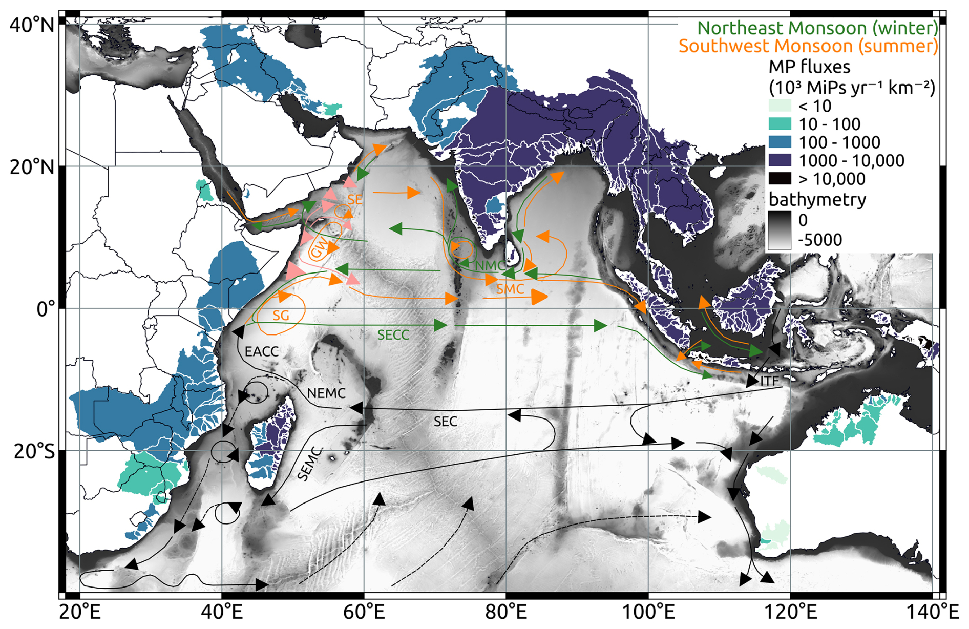
Figure A1 Spatial distribution of mean annual MiP specific fluxes (number of particles 10⁶ yr⁻¹ km⁻²) discharged by model river catchments into the IndOc domain. The estimations are based on the empirical model of Weiss et al. (2021) and HydroSHEDS river catchment delineation (Linke et al., 2019). The schematic near-surface circulation during the southwest (July–August in orange) and northeast monsoon (in green) is taken from Schott et al. (2009). Black arrows indicate annual mean flows with no seasonal reversals in the Southern Hemisphere. Current branches indicate the South Equatorial Current (SEC), South Equatorial Counter-Current (SECC), Northeast and Southeast Madagascar Current (NEMC and SEMC), East African Coastal Current (EACC), Southern Gyre (SG) and Great Whirl (GW) and associated upwelling wedges during the southwest monsoon only (pink shades), Southwest and Northeast Monsoon Currents (SMC and NMC), Indonesian Through-flow (ITF).

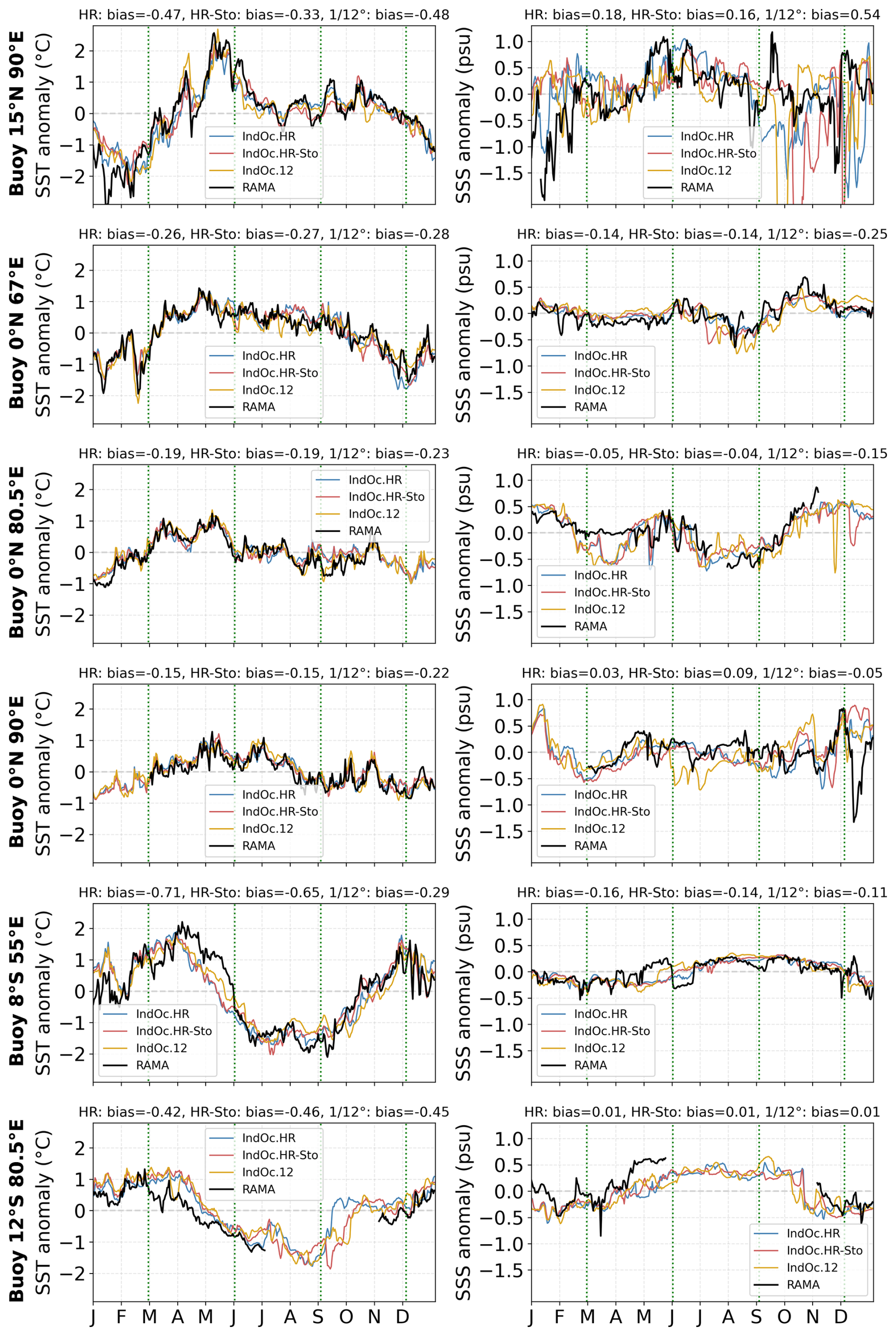
Figure A2 Daily SST and SSS time series for the year 2017 comparing the IndOc.HR, IndOc.HR-Sto and IndOc.12 simulations with in situ measurements from six RAMA buoys. The time bias for each simulation is shown above the figures. Buoy coordinates are plotted in Fig. 1.

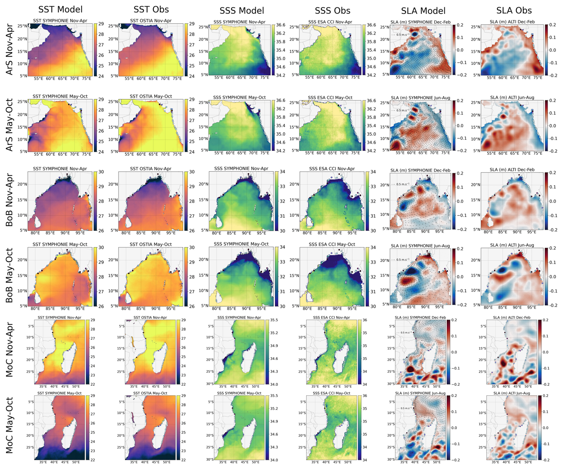
Figure A3 Spatial distribution of the averaged SST (°C, columns 1–2), SSS (psu, columns 3–4), SLA (m, columns 5–6) during the Winter Monsoon in the North, i.e. warm rainy season in the South (November–April) and Summer Monsoon in the North, i.e. cold dry season in the South (May–October), in model outputs and satellite observations for the three sub-regions: the Arabian Sea (ArS), the Bay of Bengal (BoB) and the Mozambique Channel (MoC).

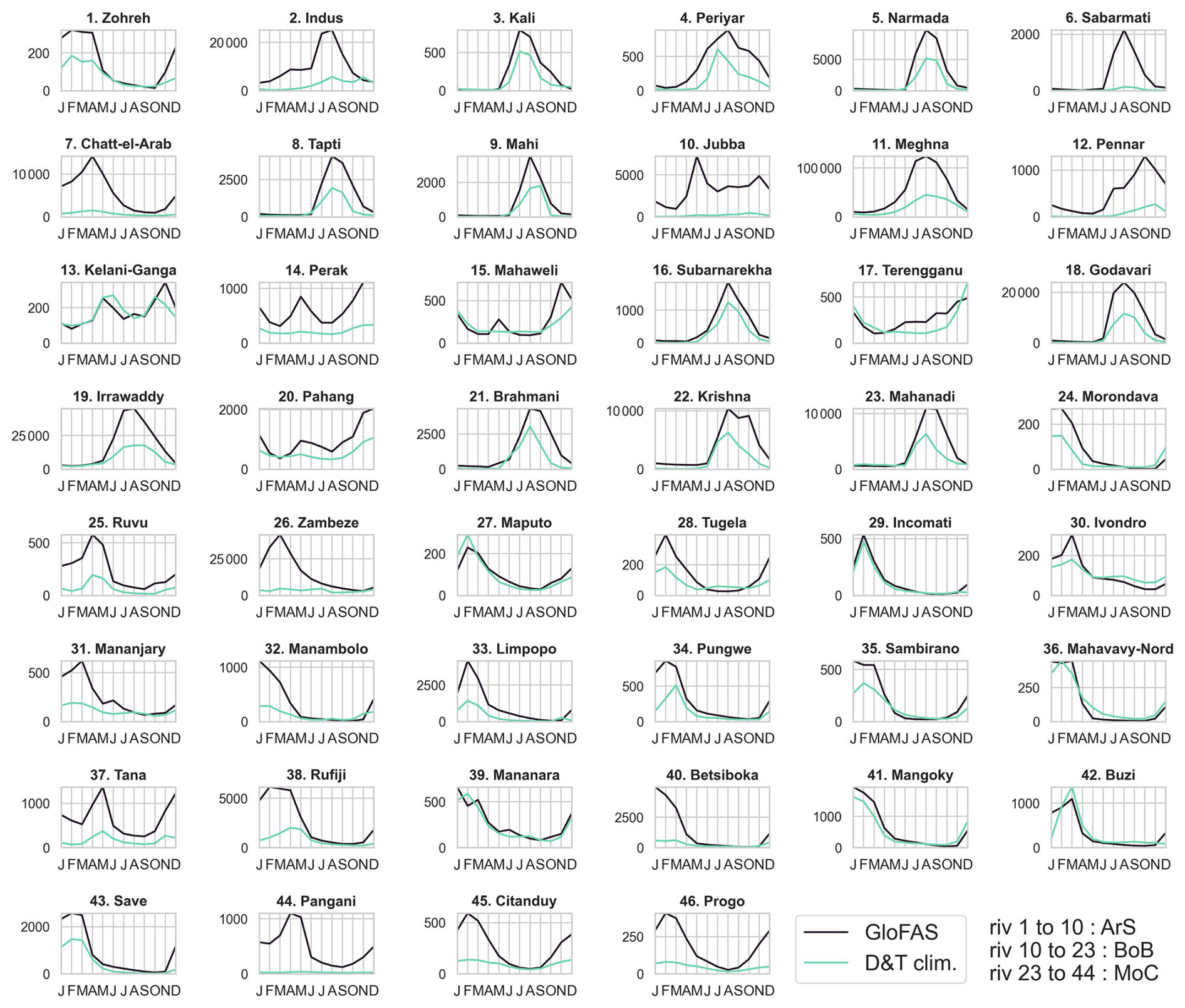
Figure A4 Time series of climatological monthly mean discharge from GloFASv3.1 forcing (over 2016–2021) and from Dai & Trenberth climatology (scattered data between 1900 and 2018 by river).

Figure A5 Seasonal spatial distribution of the MKE (Mean Kinetic Energy, Eq. A7) and EKE (Eddy Kinetic Energy, Eq. A8) from the IndOc.HR and IndOc.12 simulations, during the boreal winter (DJF) and summer (JJA) of 2017.

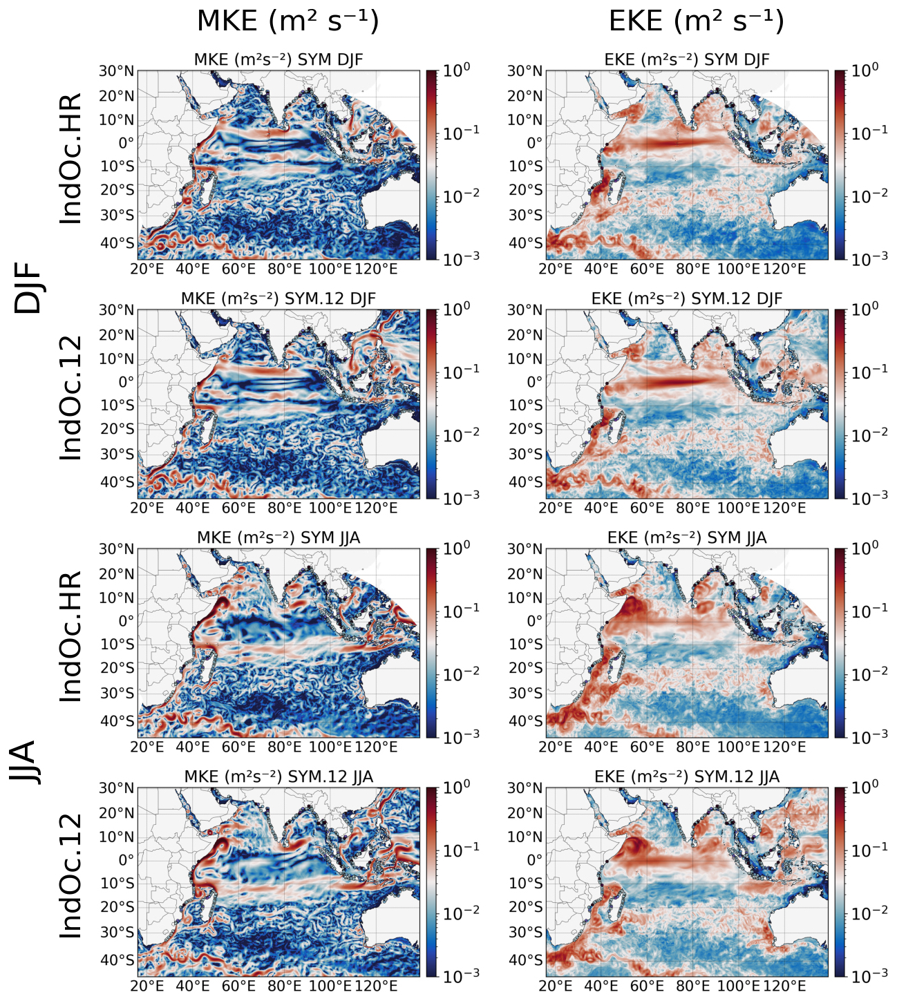
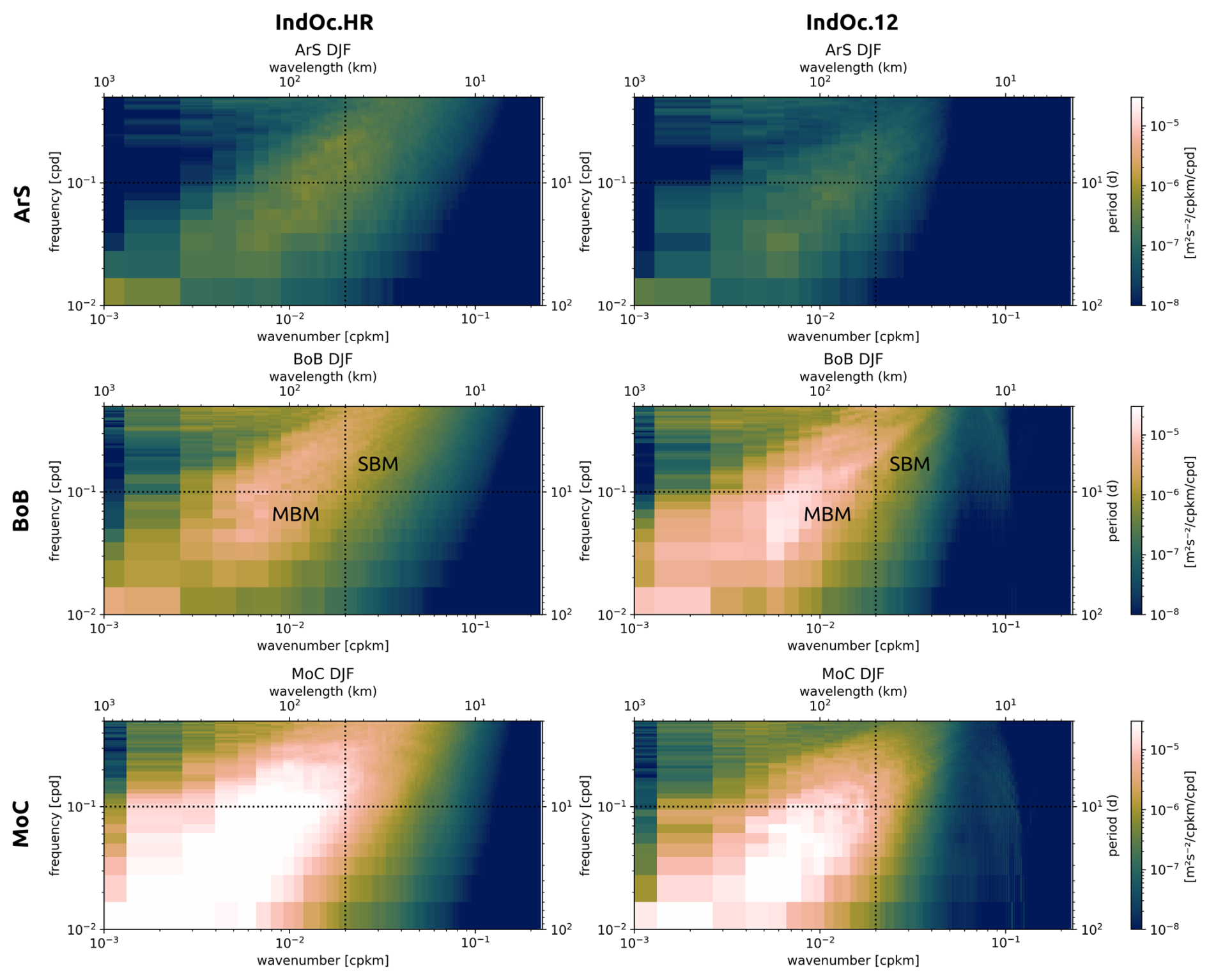
Figure A6 Frequency-Wavenumber spectra of KE (m² s⁻²) for the high (IndOc.HR, 1–3 km, blue) and low (IndOc.12, 9 km, yellow) resolution simulations over the DJF season for the three studied regions (ArS, BoB and MoC, smaller blue boxes in Fig. 1). MBM stands for mesoscale balanced, SBM for submesoscale balanced.

Figure A7 Frequency-Wavenumber spectra of KE (m² s⁻²) for the high (IndOc.HR, 1–3 km, blue) and low (IndOc.12, 9 km, yellow) resolution simulations over the JJA season for the three studied regions (ArS, BoB and MoC, smaller blue boxes in Fig. 1). MBM stands for mesoscale balanced, SBM for submesoscale balanced.

Figure A8 Monthly average Stokes drift (m s⁻¹) from the global CMEMS WAVERYS 0.2° product (CMEMS, 2019) used to force the IndOc.HR-Sto simulation.

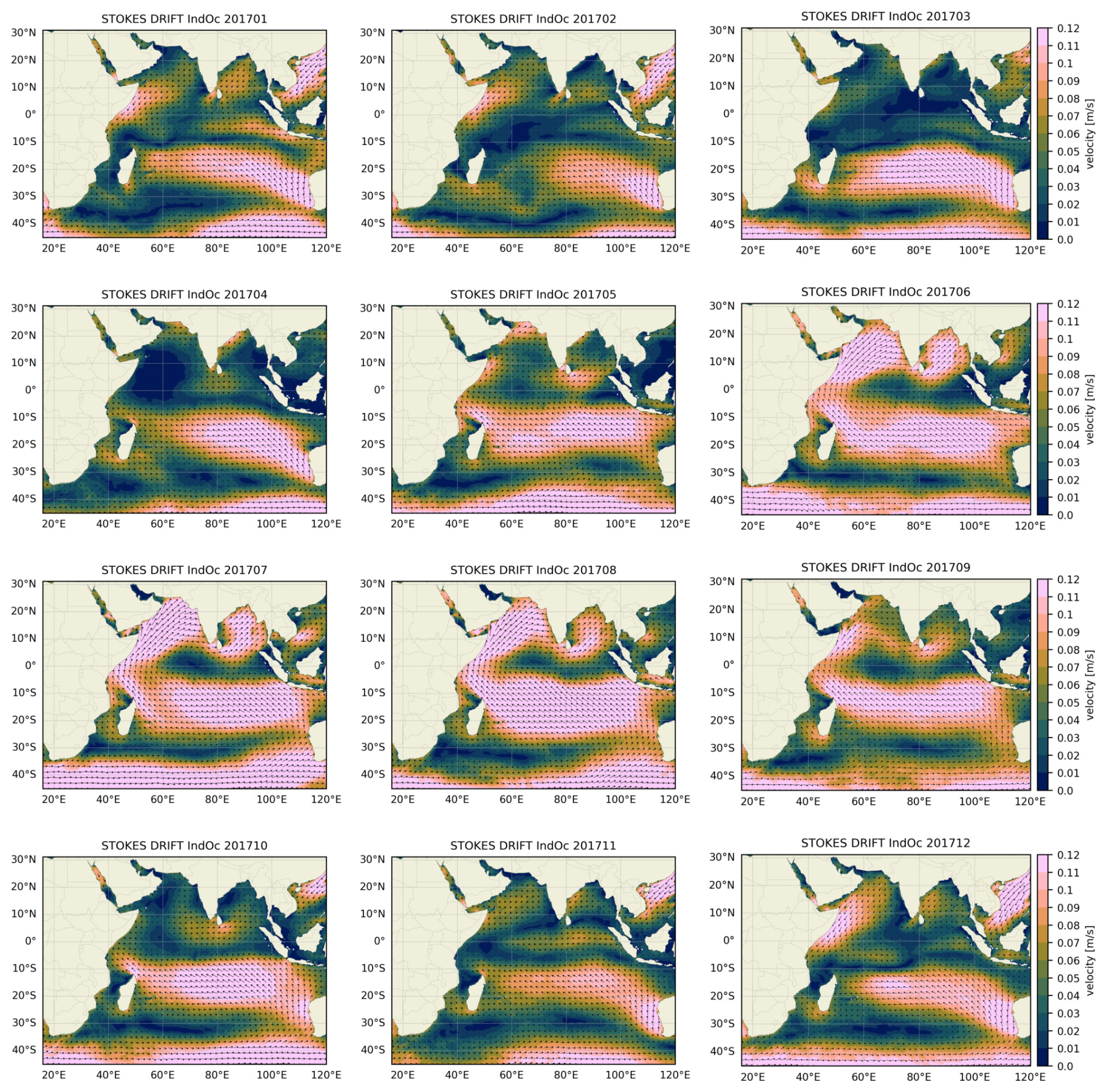
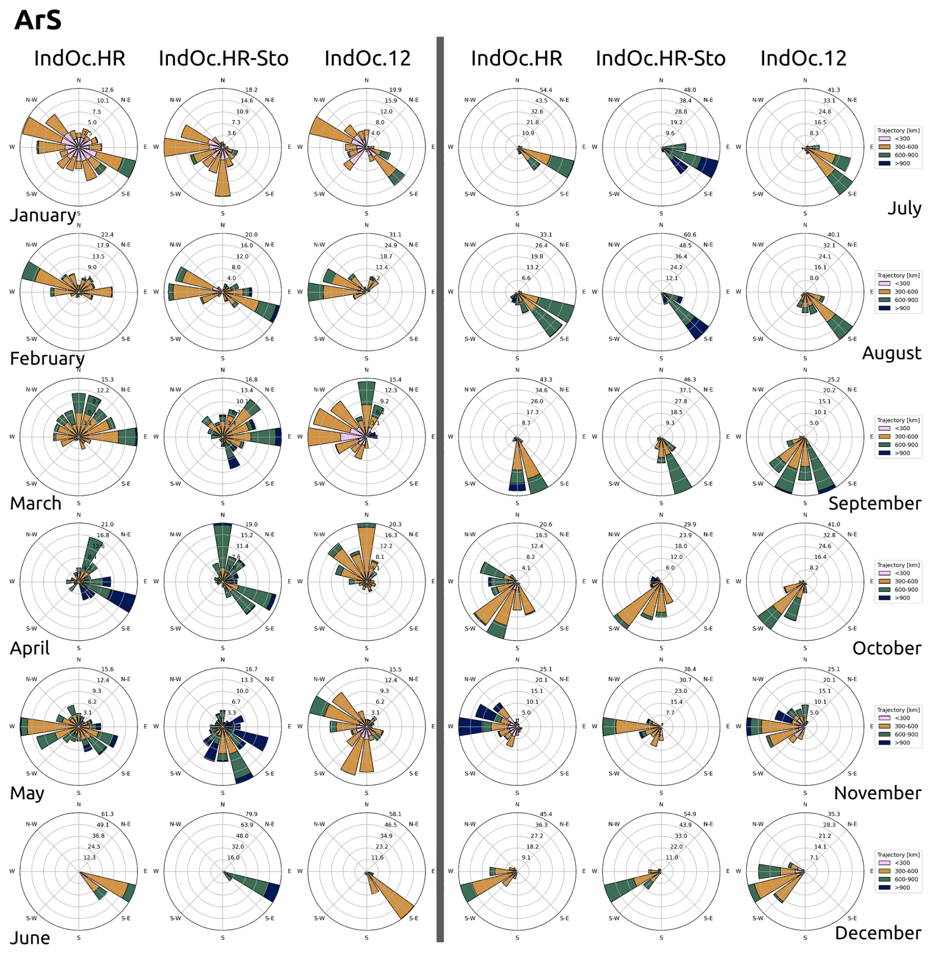
Figure A9 Monthly trajectory roses in the ArS region for the three simulations (IndOc.HR, IndOC.HR-Sto, IndOC.12). The size of the arrows indicates the frequency of particles that follow the corresponding direction. The colors indicate the length of the 30 d trajectories in the corresponding direction (pink: < 300, orange: 300–600, green: 600–900, blue: > 900 km).

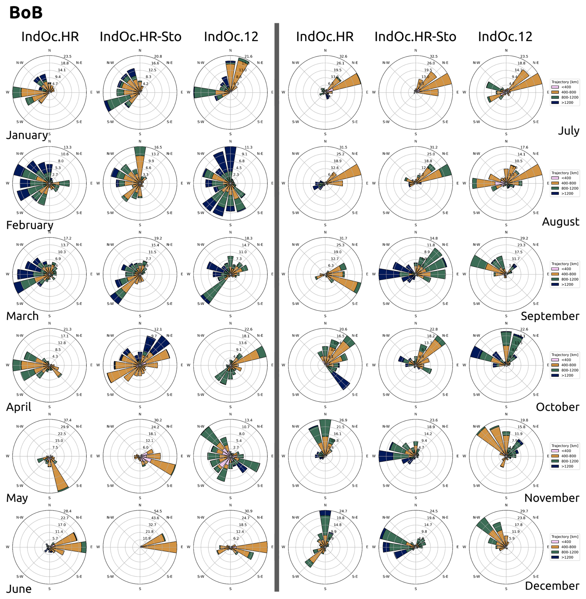
Figure A10 Monthly trajectory roses in the BoB region for the three simulations (IndOc.HR, IndOC.HR-Sto, IndOC.12). The size of the arrows indicates the frequency of particles that follow the corresponding direction. The colors indicate the length of the particle 30 d trajectories in the corresponding direction (pink: < 400, orange: 400–800, green: 800–1200, blue: > 1200 km).

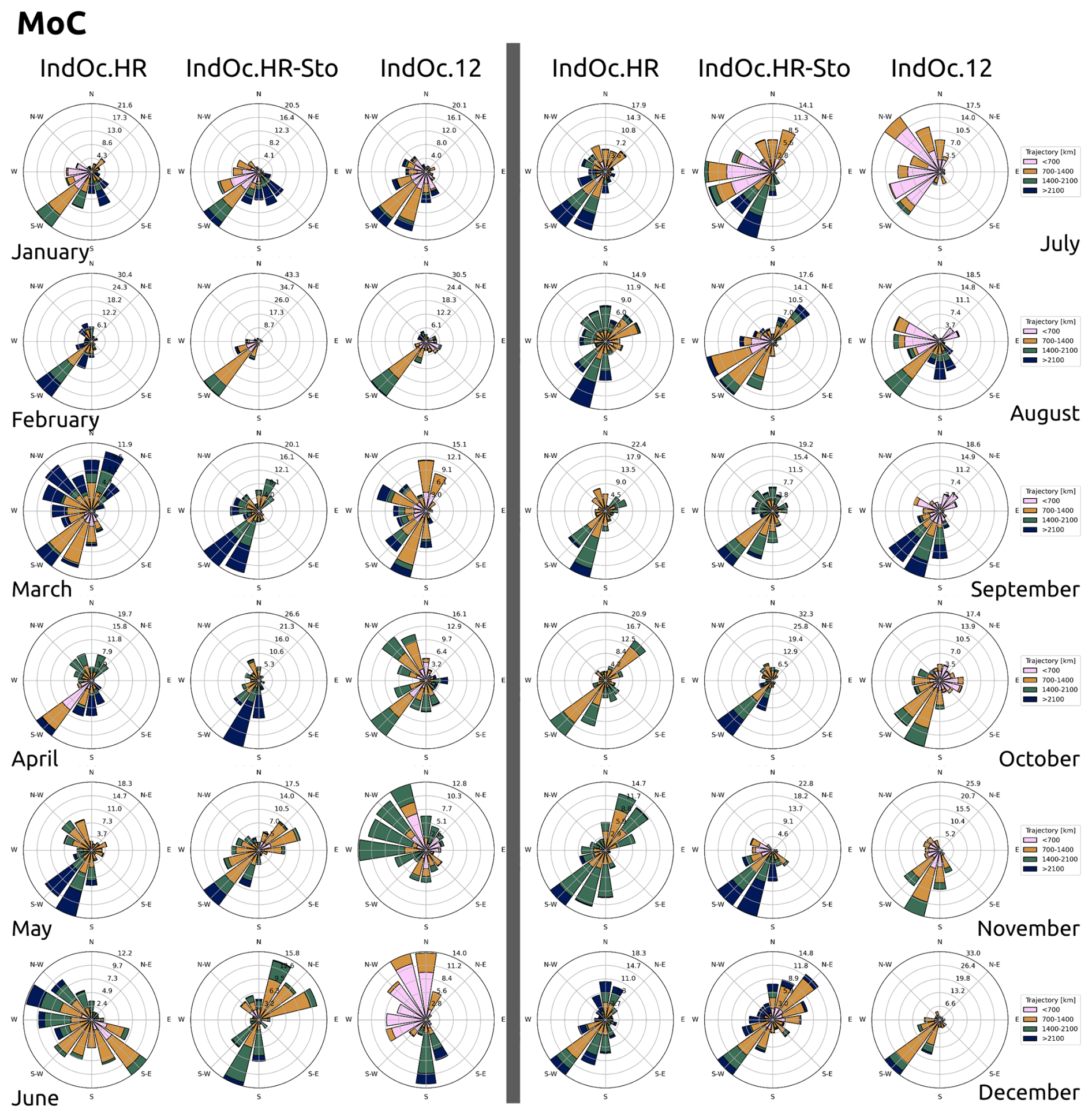
Figure A11 Monthly trajectory roses in the MoC region for the three simulations (IndOc.HR, IndOC.HR-Sto, IndOC.12). The size of the arrows indicates the frequency of particles that follow the corresponding direction. The colors indicate the length of the particle 30 d trajectories in the corresponding direction (pink: < 700, orange: 700–1400, green: 1400–2100, blue: > 2100 km).