Zooming in: SCREAM at 100 m using regional refinement over the San Francisco Bay Area

Pushing global climate models to large-eddy simulation (LES) scales over complex terrain has remained a major challenge. This study presents the first known implementation of a global model – SCREAM (Simple Cloud-Resolving E3SM Atmosphere Model) – at 100 m horizontal resolution using a regionally refined mesh (RRM) over the San Francisco Bay Area. Two hindcast simulations were conducted to test performance under both strong synoptic forcing and weak, boundary-layer-driven conditions. We demonstrate that SCREAM can stably run at LES scales while realistically capturing topography, surface heterogeneity, and coastal processes. The 100 m SCREAM-RRM substantially improves near-surface wind speed, temperature, humidity, and pressure biases compared to the baseline 3.25 km simulation, and better reproduces fine-scale wind oscillations and boundary-layer structures. These advances leverage SCREAM's scale-aware SHOC turbulence parameterization, which transitions smoothly across scales without tuning. Performance tests show that while CPU-only simulations remain costly, GPU acceleration with SCREAMv1 on NERSC's Perlmutter system enables two-day hindcasts to complete in under two wall-clock days. Our results open the door to LES-scale studies of orographic flows, boundary-layer turbulence, and coastal clouds within a fully comprehensive global modeling framework.

1 Introduction

With the rise of high-performance computing, general circulation models (GCMs) are now able to operate at convection-permitting scales – often referred to as the k-scale. Meanwhile, many studies have employed limited-area cloud-resolving or mesoscale models at large-eddy simulation (LES) scales at O(100) m. These high-resolution simulations have substantially advanced our understanding of turbulence in complex terrain, a topic of importance for local microclimates, atmospheric exchanges over mountains, renewable energy, forest fires, urban meteorology, and more (De Wekker et al., 2018). Taking renewable energy as an example: wind energy relies on boundary-layer wind and turbulence for optimal turbine siting and resource assessment; hydropower depends on snowmelt, runoff, and transpiration; solar energy is influenced by terrain shading, cloud formation, and aerosol radiative effects. To accurately simulate such processes and guide energy infrastructure deployment, resolving lower-boundary heterogeneities is crucial. A robust way to improve model reliability is to increase resolution, thereby reducing the reliance on phenomenological parameterizations.

Because high-resolution observational networks remain sparse, LES simulations often serve as a benchmark for evaluating mesoscale models and GCMs. The convergence of LES solutions is attributed to Reynolds-number similarity: once the grid spacing is sufficiently fine to resolve the dominant large eddies (i.e., those not governed by viscous dissipation) and to capture the critical turbulent motions set by the flow's Reynolds number, the statistical nature of turbulence becomes stable, changing little with further refinement. Traditional LES configurations, however, typically focus on idealized flows. Recently, researchers have adapted LES turbulence parameterizations to include realistic topography and are more tightly coupled with an interactive land model, making them suitable for realistic flows over complex terrain (e.g., Chow et al., 2006; Zhong and Chow, 2012; Arthur et al., 2018).

Over the past two decades, global circulation models have experienced a dramatic increase in horizontal resolution from around 100 km down to about 1 km, the so-called k-scale. Current k-scale global climate models (GCMs), which explicitly resolve deep convection and employ non-hydrostatic dynamics, have demonstrated substantial improvements over traditional O(100) km models – advancements that cannot be achieved through refinement of physical parameterizations alone (e.g., Stevens et al., 2019; Caldwell et al., 2021). One might ask: is it feasible to push k-scale GCMs down to LES scales? The primary challenge is that boosting a global model from a few kilometers to O(100 m) resolution demands enormous computational resources, far more than that required by limited-area models. Nevertheless, regionally refined mesh (RRM) technology holds considerable promise in this context. RRM (also referred to as variable-resolution modeling in the CESM and MPAS-A communities) allows for a smooth transition from coarse to fine horizontal resolution over targeted regions, achieving much of the benefit of high-resolution simulations at a fraction of the computational cost of globally uniform high-resolution models. (e.g., Ringler et al., 2008; Harris and Lin, 2013; Zarzycki and Jablonowski, 2014; Huang and Ullrich, 2017; Tang et al., 2019, 2023; Rhoades et al., 2023).

The Simple Cloud-Resolving E3SM Atmosphere Model (SCREAM), developed under the U.S. Department of Energy's Energy Exascale Earth System Model (E3SM) project, represents such a global 3.25 km convection-permitting model with RRM capabilities (Caldwell et al., 2021; Donahue et al., 2024). SCREAM-RRM has demonstrated good skill in simulating extreme weather events, such as derechos and atmospheric rivers (Liu et al., 2023; Bogenschutz et al., 2024), as well as in capturing the influence of complex topography and microclimates on regional climate across both historical and future periods in California (Zhang et al., 2024a).

Compared to the traditional approach of incrementally adding complexity to idealized LES models, increasing the resolution of a k-scale climate model to the LES scale offers unique advantages. Climate models inherently account for interactions between multiple components, including complex topography, interactive land processes, and turbulence-cloud interactions. Furthermore, SCREAM's hindcast configuration closely resembles operational forecasting, enabling realistic case studies by initializing from reanalysis and prescribing sea surface temperature (SST) and sea-ice cover from satellite observations. With a scale-aware turbulence scheme, it is conceptually feasible to transition from k-scale to LES resolution. Notably, the turbulence grey zone spanning O(1) km to O(100) m, features grid spacings comparable to the scale of major turbulent eddies (e.g., Langhans et al., 2012).

Physical parameterizations for microphysics and radiative transfer can, at least structurally, remain consistent across model resolutions down to micron scales, although accounting for terrain shading/reflection in radiation would be beneficial. Once Δx approaches 100 m, the effective resolution ($\approx \mathrm{6}-\mathrm{8}\mathrm{\Delta }x$) can resolve deep convective elements. Indeed, Bogenschutz et al. (2023) demonstrated that SCREAM's turbulent transport in the idealized doubly periodic f-plane configuration (DP-SCREAM) maintains reasonable scale-awareness and scale-insensitivity down to 100 m, with simulation fidelity improving as resolution increases. These findings motivate further investigation into whether SCREAM can be extended to LES scales over complex terrain and how it performs in fully comprehensive configurations.

This paper documents our efforts to push SCREAM from 3.25 km–100 m. We perform two hindcast simulations using SCREAM at a horizontal resolution of approximately 800 m over California, featuring an embedded high-resolution mesh refined to 100 m over the San Francisco Bay Area. While the focus is on the refined mesh over the Bay Area, to our knowledge, this represents the first attempt to test a GCM-based model at LES scales. While ICON (Icosahedral Nonhydrostatic) has also developed an LES version, it employs a conventional limited-area configuration (Dipankar et al., 2015). In contrast, a GCM like SCREAM must meticulously conserve energy, mass, and tracers while faithfully simulating a wide range of climate regimes. As a result, some of the challenges we identify may be specific to the GCM framework. At the same time, SCREAM-RRM avoids several limitations commonly associated with limited-area models, as discussed in this work. This paper details the modifications made to SCREAM's toolchain to support 100 m simulations, with the broader objective of enabling reproducible LES-scale SCREAM experiments across other regions of interest.

The remainder of this paper is organized as follows. Section 2 describes our methodology, including the design and setup of 100 m SCREAM-RRM for the San Francisco Bay Area, the hindcast case description, and the observational datasets used for model evaluation. The selected cases are introduced in Sect. 3. Section 4 presents simulation results, including comparisons with the 3.25 km SCREAM-RRM and observations. Section 5 summarizes the improvements, discusses remaining issues and the broader implications of this work.

2 Methods

This Methods section documents the full experimental setup used in the 3.25 km California and 100 m Bay Area SCREAM-RRM simulations. It begins with an overview of the SCREAM model and the design of the refined meshes, followed by details on topography processing, dynamical core configuration, and initialization and boundary conditions. Throughput performance metrics are then presented. The final sections describe the diagnostics, including energy spectra analysis and the observational datasets used for evaluation.

The section includes all necessary steps and technical details that made these simulations possible, organized by level of detail. Readers primarily interested in results and discussion may choose to skip the tertiary Sections.

2.1 Introduction to SCREAM

The 100 m SCREAM-RRM in this study is developed based on SCREAM version 0 (Caldwell et al., 2021). This Section provides an overview of the model configuration, including the dynamical core, subgrid-scale turbulence and other physical parameterizations, coupling with surface components, and the introduction of the C++ version.

2.1.1 Grid description and nonhydrostatic dynamical core

The default horizontal resolution of SCREAM is 3.25 km and does not have parameterized deep convection. SCREAM uses a 128-layer hybrid vertical coordinate, with vertical thickness in the boundary layer increasing from about 30 m near the surface to approximately 200 m near the top of the boundary layer. The model top is located at around 40 km. SCREAM's dynamical core is built upon the High-Order Methods Modeling Environment (HOMME), employing nonhydrostatic fluid dynamics (Taylor et al., 2020). Among the available thermodynamic variable options in HOMME, this study adopts the default configuration using virtual potential temperature. HOMME supports multiple time-stepping approaches; by default, the Horizontally Explicit Vertically Implicit (HEVI) scheme (Satoh, 2002) is discretized using a Runge–Kutta IMplicit–EXplicit (IMEX) method (Steyer et al., 2019; Guba et al., 2020). This scheme combines the KGU53 third-order explicit Runge–Kutta method (Guerra and Ullrich, 2016) for most prognostic equations with a second-order implicit Runge–Kutta method for vertically propagating acoustic waves. However, at extremely high resolution, the IMEX approach offers diminishing computational advantages and can encounter convergence challenges in the Newton iteration associated with its implicit component. Accordingly, we adopt the third-order KGU53 explicit scheme, which is commonly used in hydrostatic configurations but is also applicable to the non-hydrostatic mode, provided the time step remains below approximately 0.5 s. HOMME's dynamical core uses spectral elements with a 4×4 Gauss–Lobatto–Legendre (GLL) nodal grid within each element, referred to as GLL grids. The physical grid is subdivided into 2×2 grids, referred to as pg2 grids, uniformly distributed on each spectral element (Hannah et al., 2021).

2.1.2 Turbulence and cloud parameterization

SCREAM employs the Simplified Higher-Order Closure (SHOC) scheme as a unified parameterization for boundary-layer turbulence, cloud macrophysics, and shallow cumulus (Bogenschutz and Krueger, 2013). SHOC employs a double-Gaussian probability density function (PDF) to diagnose cloud fraction, cloud liquid water content, and buoyancy flux. The diagnosed buoyancy flux is then used to close the subgrid-scale (SGS) turbulent kinetic energy (TKE) equation. Higher-order moments for the PDF are diagnosed rather than predicted for computational efficiency. Vertical fluxes of turbulence are represented by downgradient diffusion (similar to Bretherton and Park, 2009). Eddy diffusivity is updated based on the predicted SGS TKE, consistent with Cheng et al. (2010), who suggested that when SGS TKE is accurately predicted, downgradient closures generally function well for k-scale models. Since SHOC is designed to operate across spatial scales ranging from a few hundred meters to several hundred kilometers, SHOC sets the maximum allowable value of (L) to the size of the horizontal grid mesh. In addition, L depends on SGS TKE, boundary-layer depth, eddy turnover timescale (boundary-layer depth divided by the convective velocity scale), and local stability, making it scale aware because SGS TKE typically increases with increasing Δx, thus increasing L. Phenomenologically, the maximum unresolved eddy size increases (or decreases) with the cloud depth (or buoyancy flux).

2.1.3 Microphysics, radiation, and surface coupling

The cloud fraction and cloud liquid water diagnosed by SHOC are passed to the Predicted Particle Properties (P3) microphysics scheme (Morrison and Milbrandt, 2015) and the RTE+RRTMGP radiative transfer package (Pincus et al., 2019). The cloud droplet number concentration required by the microphysics scheme and gas optical properties for radiative transfer are provided by the Simple Prescribed Aerosols (SPA) module, which includes monthly aerosol climatology from 1° E3SM simulations. State variables and radiative fluxes at the lowest atmospheric level, updated by SHOC, microphysics, and radiation schemes are subsequently passed to the coupler, interacting with E3SM's land model (ELM) (Golaz et al., 2019) and the Los Alamos sea-ice model CICE4 (Hunke et al., 2008) with prescribed-ice and a data-ocean mode. Land surface fluxes, including momentum, sensible heat, and latent heat, rely on Monin–Obukhov similarity theory, iteratively solving for bare soil/canopy temperatures and surface fluxes via an energy-balance equation. Ocean surface fluxes are computed within the coupler, with multiple options provided. This study adopts the default bulk formula which iteratively solves stability, roughness, and the bulk transfer coefficients.

2.1.4 C++ version: EAMxx

SCREAM version 1, implemented in C++ and referred to as EAMxx, has recently been documented and made publicly available (Donahue et al., 2024). Its global climatology closely resembles that of version 0 implemented in Fortran. When this study began, we only had CPU resources, EAMxx was not yet fully operational, and all simulation results presented in this paper were conducted using the SCREAMv0 Fortran version. However, during manuscript preparation, we tested the 100 m EAMxx version of SCREAM-RRM on GPU nodes of the Perlmutter cluster at the National Energy Research Scientific Computing Center (NERSC), and we present the associated performance benefits in Sect. 2.5. RRM configurations are largely compatible with both EAM and EAMxx, although EAMxx requires a different namelist structure and initial condition format.

2.2 San Francisco Bay Area 100 m SCREAM-RRM grid design

This Section describes the design of a high-resolution refined region over the San Francisco Bay Area within the SCREAM-RRM framework. Key considerations include the horizontal extent of refinement, topographic diversity, grid quality metrics, column number comparison, and tools used to generate the mesh and associated files.

2.2.1 Refined region coverage and resolution

The first-order refinement of the refined mesh used in this study covers the same domain as the 3.25 km California RRM employed by Zhang et al. (2024a) for future projections. However, in our configuration, the refined region has a horizontal resolution of 800 m over California, transitioning to 100 km outside the refined area. The 800 m refinement has been validated in Bogenschutz et al. (2024), capturing representative atmospheric river events. Building on the 800 m grid, a second-order refinement at 100 m resolution is applied over the Bay Area, extending from Drakes Bay in the north to Santa Cruz in the south, westward to the Pacific Ocean off San Francisco, and eastward to Stockton (Fig. 1). This RRM grid achieves a maximum Dinv-based element distortion metric of 3.04, indicating high grid quality (see https://acme-climate.atlassian.net/wiki/spaces/DOC/pages/872579110/Running+E3SM+on+New+Atmosphere+Grids, last access: 22 April 2025). Notably, this grid yields a global refinement factor of 1000.

2.2.2 Topographic features and regional targeting

The 100 m region required careful design. Anticipating potential applications in wind energy assessment, we ensured that the city of Livermore was included within the refined domain, thereby capturing both the Altamont Pass and Shiloh wind farms. The selected 100 m region encompasses highly heterogeneous topography, ranging from Mount Diablo (∼1000 m) and the Santa Cruz Mountains (100–1000 m) to the San Francisco Bay and the San Joaquin Valley, which lie near or below sea level (Fig. 1).

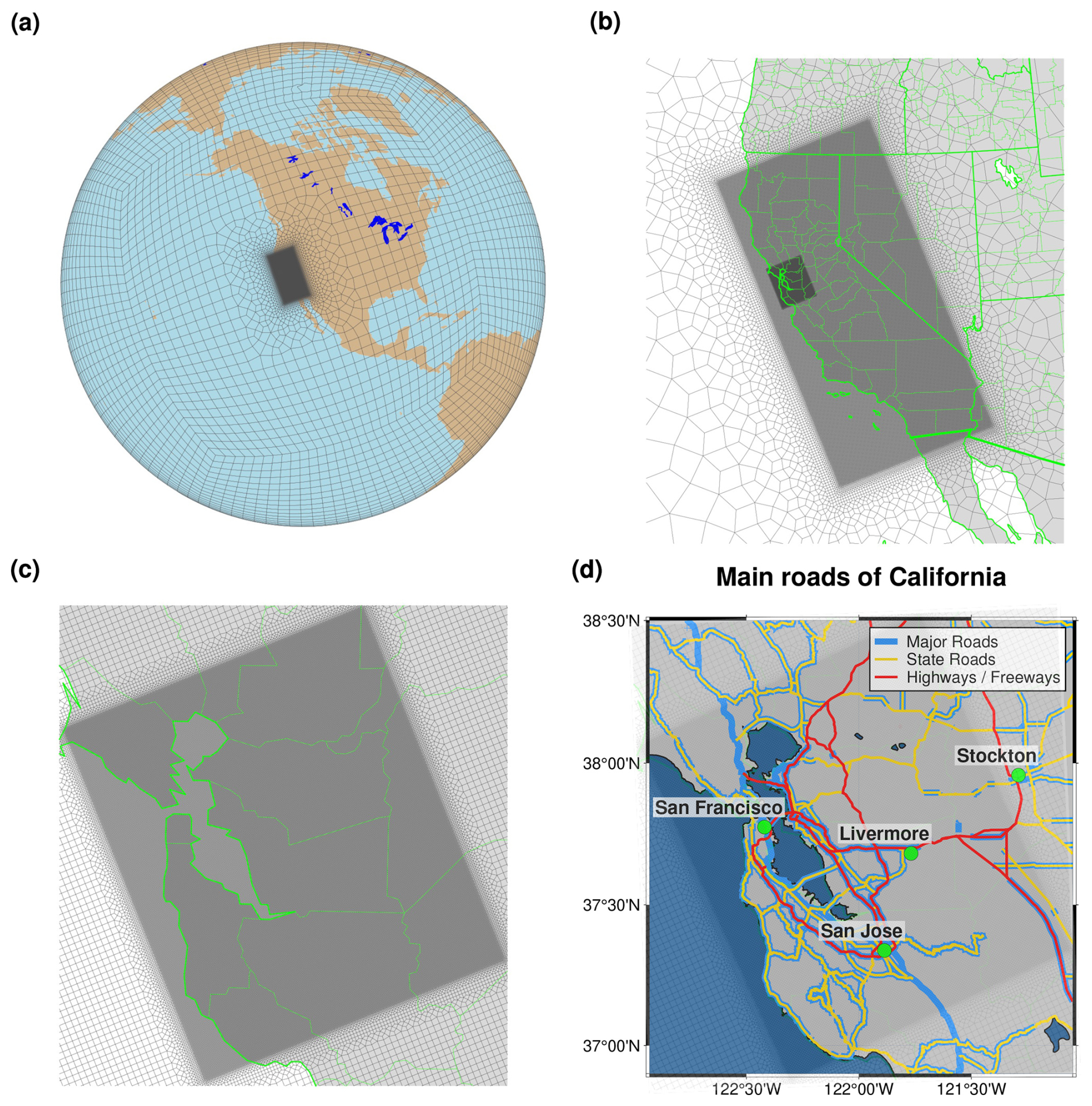
Figure 1 The regionally refined grid for (a) global view, (b) California view, (c) Bay Area view, and (d) Bay Area overlaid with roads in the 100 m SCREAM-RRM.

2.2.3 Column numbers and global proportion

Notably, the 100 m Bay Area RRM is the first known attempt to refine a global mesh down to 100 m resolution. Our primary goal is to verify the feasibility of this configuration by demonstrating its stability and its ability to produce physically credible solutions. Although our 100 m coverage cannot be extensive, our high resolution mesh covers an area of 150 km×150 km – comparable to or larger than typical DP-SCREAM or large LES domains. The 100 m RRM contains 1 333 296 physical columns, which are more than twice the number in the 800 m California RRM (587 904 columns; Bogenschutz et al., 2024) and approximately 20 times that in the 3.25 km RRM (67 872 columns; Zhang et al., 2024a), yet it accounts for only 5.3 % of the total columns in the global 3.25 km SCREAM configuration.

2.2.4 Grid generation

The land model is executed on the same grid as the atmosphere, while the ocean component uses the MPAS oRRS18to6v3 mesh (a publicly available mesh developed by the E3SM community) which provides 18 km resolution in the tropics, gradually refining to 6 km near the poles. We generated the atmosphere/land RRM grid with SQuadGen version 1.2.2 (SQuadGen, Ullrich and Roesler (2024); https://github.com/ClimateGlobalChange/squadgen, last access: 25 January 2025), with the following command:

./SQuadGen
  --output CAne32x128_Altamont100m_v2.g \
  --refine_rect "-119.8,31,-118.8,43,7;-122.3,36.9,-121.7,38.5,10" \
  --refine_level 10 --resolution 32 --smooth_type SPRING \
  --lat_ref 38 --lon_ref -116 --orient_ref 20

The grid configuration files, including the domain files and mapping files for atmosphere/land/ocean, topography, land surface data, and dry deposition file, were generated using the E3SM standalone toolchains. Topography generation is discussed in detail in the next section.

2.3 Topography generation

This Section summarizes the modifications made to the default E3SM topography workflow to enable 100 m RRM simulations. Key steps include acquiring and pre-processing 500 and 250 m global DEMs, adapting and debugging tools in the E3SM topography toolchain, addressing interpolation-related numerical issues, and tuning topography smoothing to ensure model stability.

2.3.1 High-resolution DEM acquisition and preprocessing

As part of “Running E3SM on New Atmosphere Grids” toolchain (https://acme-climate.atlassian.net/wiki/spaces/DOC/pages/872579110/Running+E3SM+on+New+Atmosphere+Grids, last access: 25 January 2025), topography generation has been modified from the NCAR topography workflow (Lauritzen et al., 2015). In the default E3SM topography workflow, new grids are generated based on the ne3000 (3.25 km) cubed-sphere topography, which is derived from the USGS GTOPO30 digital elevation model (DEM) at 30 arcsec (∼1 km) resolution. This is because most newly generated grids have coarser resolutions than SCREAM's default 3.25 km resolution. Therefore, the first step in our workflow was to obtain higher-resolution DEM data and interpolate it onto the cubed-sphere grid.

For regional modeling (such as WRF), DEM data finer than 100 m resolution is often readily available. For global grids, however, the highest publicly available DEM we found is USGS GMTED2010 at 7.5 arcsec (250 m) resolution, which lacks coverage poleward of 56° latitude (and Greenland). We obtained a publicly available 250 m GMTED2010 dataset (https://topotools.cr.usgs.gov/gmted_viewer/gmted2010_global_grids.php, last access: 25 January 2025), using a GIS tool to merge all tiles into a global lat-lon NetCDF file. GMTED2010 also provides 15 arcsec (500 m) global DEM data (Danielson and Gesch, 2011). We obtained a global 500 m GMTED2010 netcdf file by incorporating the Moderate Resolution Imaging Spectroradiometer (MODIS) MOD44W land–water mask from Jos van Geffen (personal communication, 2024, courtesy of Maarten Sneep, Koninklijk Nederlands Meteorologisch Instituut). To create a global 250 m DEM grid, we bilinearly regridded the 500 m GMTED2010 dataset and extracted the areas poleward of 56° latitude to merge with the 250 m GMTED2010 dataset. However, due to memory limitations, the 250 m DEM could not be converted to the cubed-sphere using the bin_to_cube tool in the topography workflow (e.g., at least 507 GB of memory was required). Thus, our highest feasible DEM resolution is 500 m.

2.3.2 Topography mapping to the 100 m RRM grid

Using the 500 m DEM, we successfully generated an 800 m base cubed-sphere topography by fixing a bug in E3SM's bin_to_cube tool and switching the NetCDF output format to NF_64BIT_DATA. We also conducted additional preprocessing steps (e.g., reclassifying the land–water mask), although these are not required in the current E3SM workflow. The 800 m base cubed-sphere topography was subsequently mapped onto the target 100 m RRM GLL (dynamical core) and pg2 (physics) grids using the cube_to_target tool, which currently offers the most efficient and practical approach. During this step, we encountered a bug where the generated RRM exhibited anomalously large negative topography values at specific, non-adjacent grid points. As a temporary solution, we replaced these outliers by taking the arithmetic mean of their neighbors. Further investigation revealed negative weights in the overlapping regions between the base cubed-sphere grid and the target grid, particularly when the target grid was smaller than the base cubed-sphere grid. We identified a corner-case condition in the cube_to_target tool's line-integration logic that mischaracterized very short segments (where dx, dy≈0). This condition was originally intended to handle lines nearly parallel to latitude (i.e., when dy<fuzzy_width, which defaults to $\mathrm{1}\times {\mathrm{10}}^{-\mathrm{8}}$). Disabling this condition eliminates the occurrence of negative weights. Since exact integration is not essential in this context, we recommend commenting out this condition in future use.

The remainder of the topography workflow followed the E3SM Version 3 topography best practices (https://acme-climate.atlassian.net/wiki/spaces/DOC/pages/2712338924/V3+Topography+GLL+PG2+grids, last access: 25 January 2025), with the exception that we omitted the second cube_to_target call to accelerate file generation. This step is only required for the subgrid-scale gravity wave drag and turbulent mountain stress parameterizations, as it computes elevation variances across scales above and below a critical wavenumber. Since SCREAM version 0 (the model used in this study) does not include either of these parameterizations, this step was not necessary. According to linear theory, the separation scale between gravity waves and drag generated by unstratified turbulent flow depends on obstacle horizontal scale (Lauritzen et al., 2015). As resolution increases to 100 m, the small-scale drag induced by turbulent flow is expected to be explicitly resolved rather than parameterized.

2.3.3 Topography smoothing and numerical stability tests

One of the most crucial steps in the workflow was the smoothing of the RRM topography. Using the recommended six smoothing iterations led to an immediate crash at the model's first timestep, even after significantly reducing the dynamical core timestep to one-tenth of the Courant–Friedrichs–Lewy (CFL) limit and to one-tenth of the value used in the 100 m DP-SCREAM simulations (Bogenschutz et al., 2023). These early tests were conducted on a bomb cyclone hindcast event that made landfall in California, characterized by strong synoptic winds. In contrast, a sensitivity test using a finer 100 m mesh – which did not include the steep topographic gradients present in the RRM configuration examined in this study – ran successfully with the six smoothing iterations. Thus, we suspect that steep topography is the culprit for numerical instability. Eventually, we doubled the smoothing factor to 12 (matching the V2 topo guidelines) and successfully ran the bomb cyclone case at a 0.025 s dynamical core timestep. Further doubling the smoothing factor to 24 allowed the simulation to run with a timestep of 0.05 s. Notably, in a sensitivity experiment we conducted, switching the dynamical core to hydrostatic mode allowed the model to run with a topography smoothing factor of 6 and a time step of 0.25 s.

With regards to the non-hydrostatic dynamical core, fixing the negative weighting problem mentioned earlier slightly delayed instability onset, enabling simulations to reach model step 8 before crashing when using a 0.05 s timestep. Similar challenges with numerical stability due to increased resolution over complex topography have been documented in the LES community (e.g., Connolly et al., 2021). Steeper topographic gradients at finer resolutions necessitate shorter time steps than what guidance from the CFL criterion might suggest. Here, we needed a tenfold reduction in timestep, implying additional adjustments may be required for SCREAM's non-hydrostatic dynamical core at 100 m (e.g., a scale-aware sponge layer). Alternatively, regridding a coarser DEM onto a finer grid might introduce blocky mountains or steep gradients at the boundaries around DEM elements that exacerbate instabilities.

Figure 2 compares the topography of the 3.25 km California RRM and the 100 m Bay Area RRM.

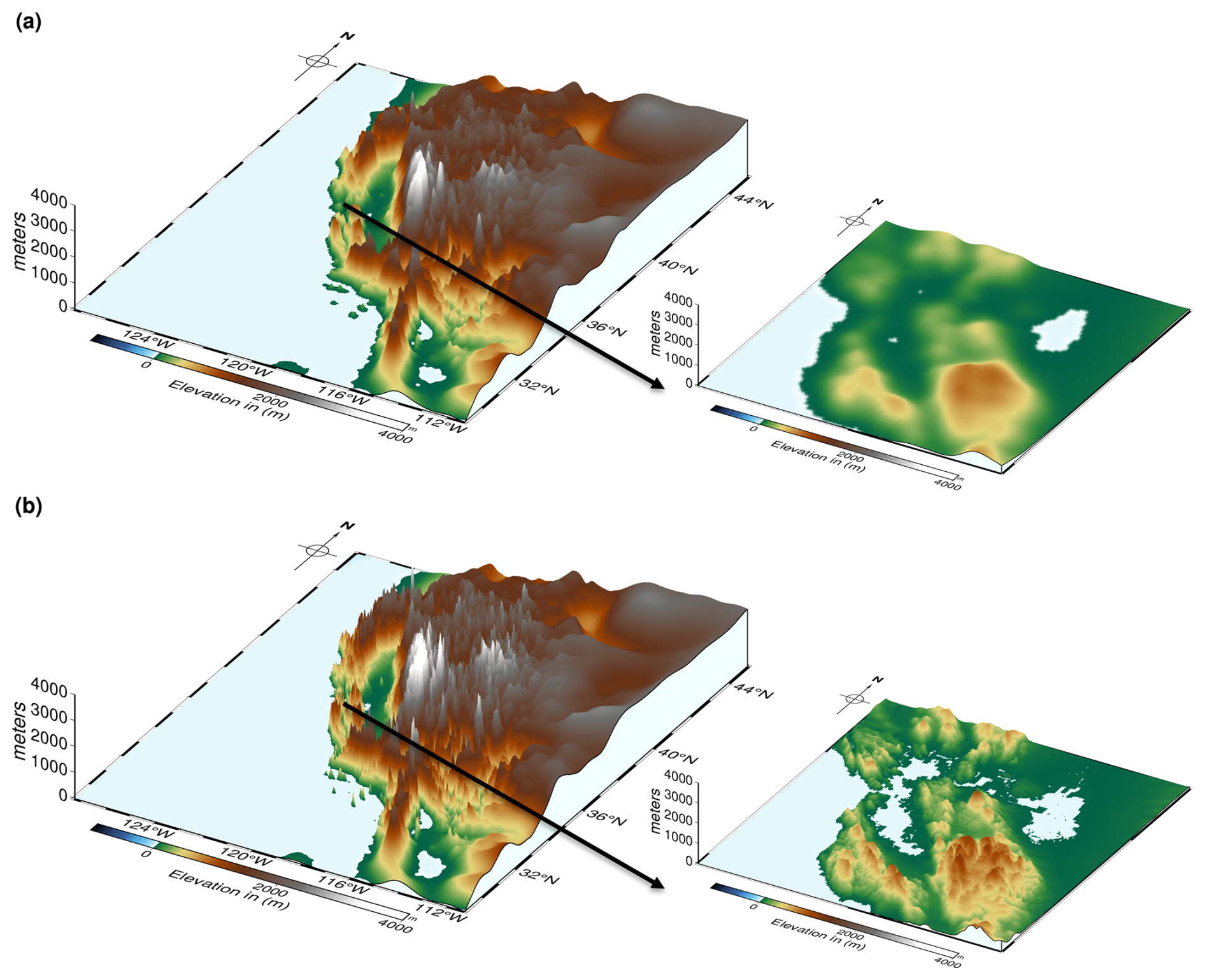
Figure 2 The topography of the (a) 3.25 km California RRM and (b) 100 m Bay Area RRM. Each is shown with both a full California overview and a bird's-eye view of the Bay Area.

2.4 Dynamical core configuration

The final namelist for the dynamical core configuration is as follows:

• Topography smoothing: 12 iterations

• Turn on topography improvement options: pgrad_correction=1, hv_ref_profiles=6

• Dycore timestep: se_tstep = 0.025 s, which is 1/10th of what we would expect from the CFL limit and 1$/$10th of what was used in in Bogenschutz et al. (2023) for 100 m DP-SCREAM simulations

• Time-stepping method: tstep_type = 5 (fully 3rd order accurate KGU53 explicit method)

• Hyperviscosity coefficient: nu $=\mathrm{3.4}\times {\mathrm{10}}^{-\mathrm{7}}{\mathrm{s}}^{-\mathrm{1}}$ (10 times the default value)

• Top-of-model sponge layer coefficient:
  nu_top = 333.34

• Tracer advection timestep: dt_tracer_factor = 8

• Lagrangian vertical level remap timestep:
  dt_remap_factor = 2

• Hyperviscosity subcycles: hypervis_subcycle = hypervis_subcycle_q = hypervis_subcycle_tom = 1

• Hyperviscosity scaling: hypervis_scaling = 3.0

Among these, topography smoothing and the dynamical core timestep are most critical for model stability.

2.5 Initialization

This Section describes the initialization procedures for both the atmosphere and land models in the simulations. The atmosphere is initialized using high-resolution ERA5 native-grid reanalysis data. The land initial condition is generated through a 5 year land-only spinup simulation driven by ERA5 atmospheric forcing. In addition, we conducted 10-member ensembles for both events in the 3.25 km California RRM.

2.5.1 Atmospheric initial conditions

The atmosphere initial conditions were derived from the Fifth Generation European Centre for Medium-Range Weather Forecasts Reanalysis (ERA5) High Resolution (HRES) global reanalysis data (Hersbach et al., 2020), which has a native horizontal resolution of 31 km (0.28125°). The variables are stored with T639 triangular truncation (spectral resolution) or a reduced Gaussian grid with a resolution of N320. Vertically, it uses a 137-layer hybrid pressure/sigma coordinate that affords ∼20 m resolution near the surface and ∼130 m at 850 hPa, closely matching SCREAM's default 128-layer vertical coordinate in the lower and middle troposphere. We chose this native-grid ERA5 dataset over the more commonly used pressure-level lat-lon dataset to better align with SCREAM's vertical grid, especially given the critical role that fine vertical resolution plays in stratocumulus simulations (e.g., Lee et al., 2022; Bogenschutz et al., 2023).

Since we were using ERA5 HRES native-grid data, the CAPT package (https://github.com/PCMDI/CAPT, last access: 25 January 2025) was used to generate the atmosphere initial conditions, including horizontal interpolation onto SCREAM's GLL grid, adjustment of surface pressure, and vertical interpolation onto the 128-layer hybrid coordinate. Alternatively, the HICCUP package (https://github.com/E3SM-Project/HICCUP, last access: 25 January 2025), which is frequently used in the E3SM/SCREAM community (e.g., Zhang et al., 2024a; Bogenschutz et al., 2024; Zhang et al., 2024b), would be convenient if using ERA5 pressure-level data. CAPT requires Earth System Modeling Framework (ESMF) software (https://earthsystemmodeling.org/regrid/, last access: 25 January 2025) for horizontal interpolation, and the target GLL description file used for ESMF can be obtained from the E3SM's homme tool. HICCUP performs horizontal interpolation by calling netCDF Operator (NCO) (Zender, 2008), which has several built-in horizontal mapping software including NCO, TempestRemap (Ullrich and Taylor, 2015), ESMF, and Climate Data Operator (CDO) (https://code.mpimet.mpg.de/projects/cdo, last access: 25 January 2025).

CAPT's vertical interpolation follows European Centre for Medium-Range Weather Forecasts (ECMWF) Integrated Forecasting System (IFS) Documentation CY23R4 (https://www.ecmwf.int/sites/default/files/elibrary/2003/77032-ifs-documentation-cy23r4-part-vi-technical-and-computational-procedures_1.pdf, last access: 25 January 2025), applying linear/quadratic/linear+quadratic interpolation for temperature/moist variables/wind, respectively. HICCUP calls NCO, using the linear to log(pressure) vertical interpolation by default. Both CAPT and HICCUP apply surface adjustment based on the Trenberth et al. (1993) procedure, which calculates the model surface pressure based on the difference in surface geopotential height (PHIS) between ERA5 and the model topography and assume dry hydrostatic lapse rate. After subtly modifying HICCUP's surface adjustment code (specifically in the choice of PHIS used in the calculation) we verified that the resulting initial conditions successfully passed a one-hour test under the previously described dynamical core configuration. For comparison, the simulation initialized with native-grid data using CAPT showed less pronounced surface adjustments and weaker horizontal grid imprinting than the one initialized with pressure-level data using HICCUP. These differences reflect the inherent distinctions between using pressure-level versus native-grid ERA5 data; however, they do not affect the model's numerical stability.

2.5.2 Land initialization and spin-up

A physically consistent land initial condition for a hindcast typically requires a multi-year spin-up driven by reanalysis atmospheric forcing. Following the workflow used in betacast (Zarzycki et al., 2014), we conducted a 5 year land-only (i.e., I-compset) simulation using ERA5 atmospheric forcing to generate the land initial condition. This I-compset simulation did not use a cold start; instead, it was initialized from an interpolated land restart file derived from a well-spun 1° E3SMv1 historical simulation (1850–2015), using the state at 1 January 2015 00:00 UTC. The interpolation process required two existing land restart files on the 3.25 km and 800 m CARRM grids, obtained from prior one-hour test simulations initialized with a cold-start land state. The ERA5 forcing data, provided at 0.25° resolution and 6 h intervals, include precipitation, downward shortwave and longwave radiation, 2 m temperature and humidity, 10 m wind, and surface pressure. Following the Betacast workflow, these data were converted into the data-atmosphere stream file format used by E3SM I-compsets. The land model uses a timestep of 1800s in the land-only simulations, consistent with the 6 h atmospheric forcing from ERA5. In the atmosphere–land coupled simulations, the land model runs with the same timestep as the atmospheric physics, which is 75 s.

2.5.3 Sensitivity to initial condition

In addition to the single-realization control runs, we conducted small ensembles (10 members each) for both events in the 3.25 km California RRM to quantify sensitivity to small perturbations in the initial conditions. Ensembles were generated by adding random perturbations of order 1⁻¹⁴ to the initial temperature profiles at all grid points. Due to computational resource constraints, we were unable to perform ensemble simulations for BA-100 m.

2.6 SST and sea ice extent

SST and sea ice extent were obtained from NOAA Optimal Interpolation (OI) data (Reynolds et al., 2007). The OISST data were preprocessed by filling missing land values using a relaxed Poisson equation, while preserving their native 0.25° resolution. The data were then reformatted into the data-ocean stream file format (https://esmci.github.io/cime/versions/ufs_release_v1.1/html/data_models/data-ocean.html, last accessed: 25 January 2025). During runtime, SCREAM interpolates the SST and sea ice fields to the model's ocean grid.

2.7 Throughput

Because of the extremely small dynamical core time step (0.025 s) needed to ensure numerical stability, and limitations on the total number of nodes per job submission, each simulation achieves a throughput of approximately one simulated hour per 6.4 wall-clock hour. On Livermore Computing's Ruby cluster, each submission utilizes 180 Intel Xeon CLX-8276L (2.2 GHz) CPUs, each with 28 cores and 192 GiB of memory, resulting in a throughput of approximately 0.16 simulated days per day (SDPD). Accounting for both runtime and queue delays, a single hindcast typically requires about one month to complete.

While preparing this manuscript, performance scaling tests were conducted for SCREAM version 1 (C++ implementation) on GPU nodes of NERSC's Perlmutter system. Each node contains four NVIDIA A100 GPUs (Ampere architecture, 40 GiB each) and four HPE Slingshot 11 NICs. We performed one-hour SCREAM-RRM simulations at 100 m resolution, scaling from 32–1024 nodes. The performance results are shown in Fig. 3. These findings underscore the critical importance of GPU acceleration for enabling ultra-high-resolution simulations. While such runs are nearly infeasible on CPU-only systems – requiring up to a month to complete – they become substantially more tractable on GPU platforms, with total runtimes reduced to less than two wall-clock days. We note that we used SCREAMv0 in this work because the full RRM capabilities for SCREAMv1 were not yet scientifically validated at the time this study was performed.

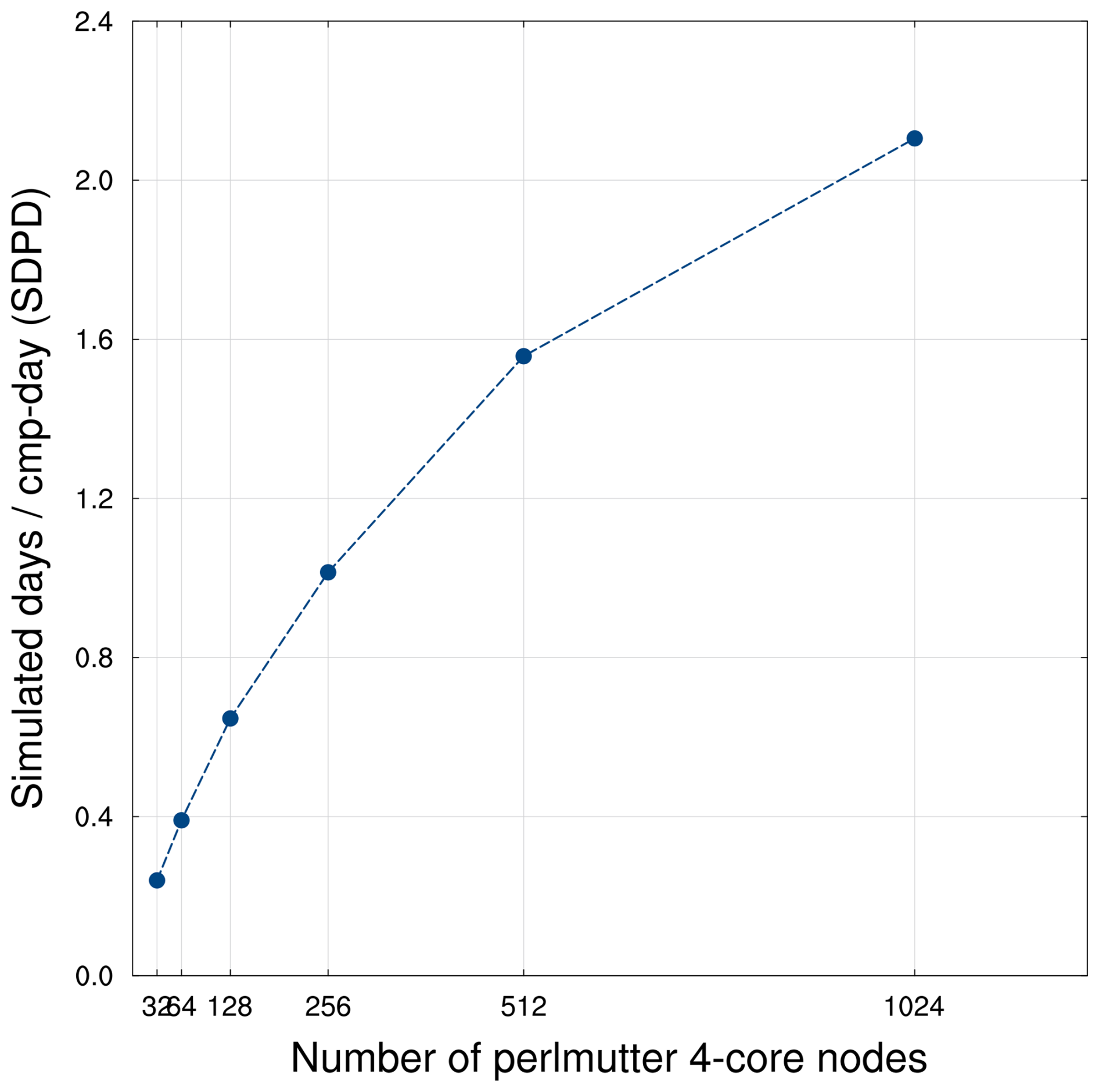
Figure 3 Performance scaling of the 100 m Bay Area SCREAMv1-RRM using the GPU nodes of the NERSC Perlmutter machine.

2.8 Energy spectra

For global models, spherical harmonics are a natural method for spectral decomposition, but they are not suitable for limited-area regional models and RRMs. For regional outputs, Discrete Fourier Transforms (DFT) and Discrete Cosine Transforms (DCT) are commonly used. DFT requires detrending or windowing, while detrending can artificially remove large-scale gradients, and windowing can distort spectra for already periodic fields (Errico, 1985; Denis et al., 2002). DCT mirrors the field to ensure symmetry before applying a Fourier transform, and is reliable for fields with spectral slopes between −4 and 1. DCT was originally developed for digital image, audio, and video compression (e.g., JPEG), but it has also been used to diagnose energy spectra in numerical simulations (e.g., Denis et al., 2002; Selz et al., 2019; Prein et al., 2022).

We used the scipy.fft package (https://docs.scipy.org/doc/scipy/tutorial/fft.html, last access: 17 September 2025) for Discrete Cosine Transforms. Since we only output high-frequency relative vorticity, divergence, and w profiles, we computed rotational and divergent KE spectra as well as w spectra at every level using 10 min instantaneous outputs. The raw outputs were on the dynamical GLL grid; they were horizontally interpolated using the NCO-native first-order conservative algorithm to 0.03° (3.25 km California RRM) and 0.001° (100 m Bay Area RRM) over the small domain of the 100 m mesh (237.5–238.5° E, 37.3–38.3° N), and vertically interpolated to SCREAM's 128 reference pressure levels using NCO's default method. The two-dimensional spectra were projected onto the zonal and meridional directions, then averaged in time (from the 6th simulation hour to the end of the simulation) and in the vertical (within 100 hPa around 200, 500, and 850 hPa, respectively).

2.9 Observation data

2.9.1 Observation datasets

Within the 100 m refinement region, we use the following in-situ observations for validation:

• World Meteorological Organization (WMO) Station Data: 6 h meteorological data from Meteomanz (http://www.meteomanz.com/, last access: 25 January 2025), including near-surface temperature, wind, and relative humidity.

• Integrated Surface Dataset (ISD) from the National Centers for Environmental Information (NCEI) website (https://www.ncei.noaa.gov/products/land-based-station/integrated-surface-database, last access: 25 January 2025), which offers 30 min, 1 h, 6 h, or longer intervals. Variables include near-surface temperature, wind, and humidity.

• NOAA Tides and Currents Meteorological Observations from NOAA Center for Operational Oceanographic Products and Services stations (https://tidesandcurrents.noaa.gov/, last access: 25 January 2025), providing 6 min surface pressure, near-surface wind and temperature.

• Integrated Global Radiosonde Archive (IGRA) from NCEI (https://www.ncei.noaa.gov/products/weather-balloon/integrated-global-radiosonde-archive, last access: 25 January 2025), at irregular temporal resolution, providing vertical profiles of pressure, temperature, humidity, and wind. This is the only publicly available source of vertical profiles for our analysis.

To our knowledge, no publicly available gridded, observation-driven meteorological products for California offer spatial resolutions finer than 3.25 km. For instance, both the Parameter-elevation Regressions on Independent Slopes Model (PRISM; https://prism.oregonstate.edu, last access: 17 September 2025) and the High-Resolution Rapid Refresh analysis (HRRR) (Dowell et al., 2022) have resolutions of 4 km. These datasets are inappropriate for evaluating numerical models at 100 m (cf. Lundquist et al., 2019) and are thus excluded from this study.

For the Stratocumulus2023 case, due to the lack of coastal soundings for cloud hydrometeors, we compare SCREAM-RRM to GOES-East/West LWP-Best Estimate imagery provided by the Satellite Cloud and Radiation Property Retrieval System (SatCORPS) https://satcorps.larc.nasa.gov/, last access: 25 January 2025), as shown in Fig. 6.

2.9.2 Data processing and model comparison

Most temperature/humidity sensors are mounted at a height of 2 m, while anemometers are deployed near 10 m. Hence, we evaluate 2 m temperature, 2 m relative humidity, 10 m wind speed, and surface pressure. Each site is matched to the nearest model gridpoint using sklearn.neighbors.BallTree (https://scikit-learn.org/1.6/, last access: 25 January 2025) within the 100 m bounding box (W: 237.07°, E: 238.95°, S: 36.9°, N: 38.5°; see Fig. 1). Note that due to the oblique orientation of the 100 m refinement area, the grid resolution at the box boundaries can locally approach 800 m, e.g., Stockton in Meteomanz/ISD. Figure 4 shows the station distributions in each dataset. Although Meteomanz and ISD datasets include precipitation, their sparse spatial coverage and coarse temporal resolution limit their usefulness for meaningful precipitation comparisons. For example, no precipitation rates exceeding 5 mm h⁻¹ were recorded during the Storm2008 case. The Tides and Currents data were downloaded using noaa_coops package (https://github.com/GClunies/noaa_coops, last access: 25 January 2025), while other datasets were retrieved directly from their websites.

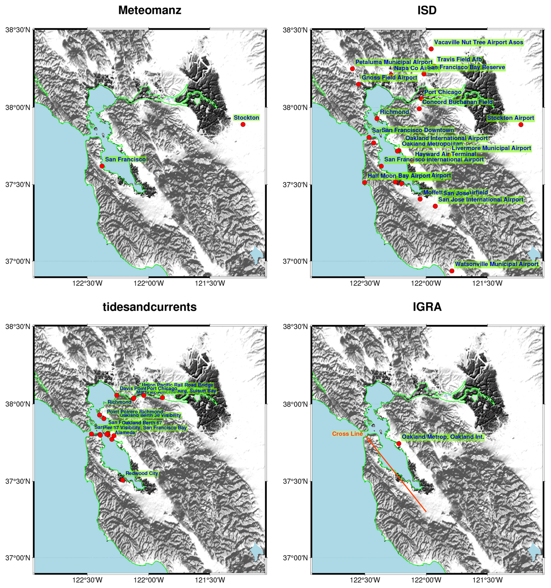
Figure 4 The spatial distribution of Meteomanz, ISD, Tides and Currents, and IGRA stations within the Bay Area, in that order.

The first three datasets (Meteomanz, ISD, and Tides and Currents) were used to calculate skill scores, including the Pearson pattern correlation coefficient, root mean squared error (RMSE), and bias. Meteomanz are available every 6 h, and Tides and Currents provide data every 6 min. ISD lacks consistent temporal resolution and is reindexed to 30 min by filling in the missing value in the metric calculations. The model's 5 min instantaneous outputs were resampled to match the observational time sampling. For Meteomanz and ISD, we extracted instantaneous values aligned with observation times and calculated the standard deviation within each observational window. For Tides and Currents, the 5 min outputs were averaged to 6 min intervals. For comparisons with IGRA, model time slices were aligned with the elapsed time of the radiosonde launches. The IGRA soundings were vertically interpolated using a log(pressure)–log(pressure) method to SCREAM's 128-layer reference pressure levels, which are defined by midpoint pressures ranging from 998.5 hPa near the surface to 2.6 hPa at the model top. For sounding comparisons, model data were interpolated to the same reference pressure levels, computed from the simulated surface pressure and hybrid sigma-pressure coefficients. Soundings were visualized using the MetPy package (https://github.com/Unidata/MetPy, last access: 25 January 2025).

3 Case description

California exhibits a diverse range of microclimates, shaped by distinct seasonal weather patterns. During winter, the region experiences hydrological events primarily driven by atmospheric rivers and midlatitude cyclones, characterized by strong synoptically forced winds. In contrast, summer conditions are dominated by marine stratocumulus clouds, influenced by large-scale subsidence associated with persistent high-pressure ridges, and are typically governed by weak synoptic forcing and locally driven circulations. In this study, we selected two representative 2 d cases corresponding to these typical weather conditions to evaluate the performance of the 100 m SCREAM-RRM under strong and weak synoptic flows.

3.1 Storm2008

The first case is initialized at 00:00 Z on 4 January 2008, and runs for 48 h, capturing “Storm 3” from the January 2008 North American storm complex. This storm underwent explosive intensification, producing wind gusts exceeding 44 m s⁻¹, total precipitation amounts up to 250 mm, and snowfall accumulations reaching 1800 mm in parts of California. We refer to this case as Storm2008. Meteorological observations from National Oceanic and Atmospheric Administration (NOAA) (https://tidesandcurrents.noaa.gov/met.html, last access: 25 January 2025) indicate average gusts near 20 m s⁻¹ and mean wind speeds around 15 m s⁻¹ at Redwood City station (station 9414523), with a minimum sea-level pressure below 1000 hPa. Storm 3 was noteworthy for reaching 956 hPa sea-level pressure, making it the strongest storm ever recorded on the West Coast at that time. Figure 5 illustrates the atmospheric river impacting California at 4 January 2008 18:00 Z, as simulated by the 3.25 km (left) and 100 m (right) SCREAM-RRMs, along with the associated precipitation patterns.

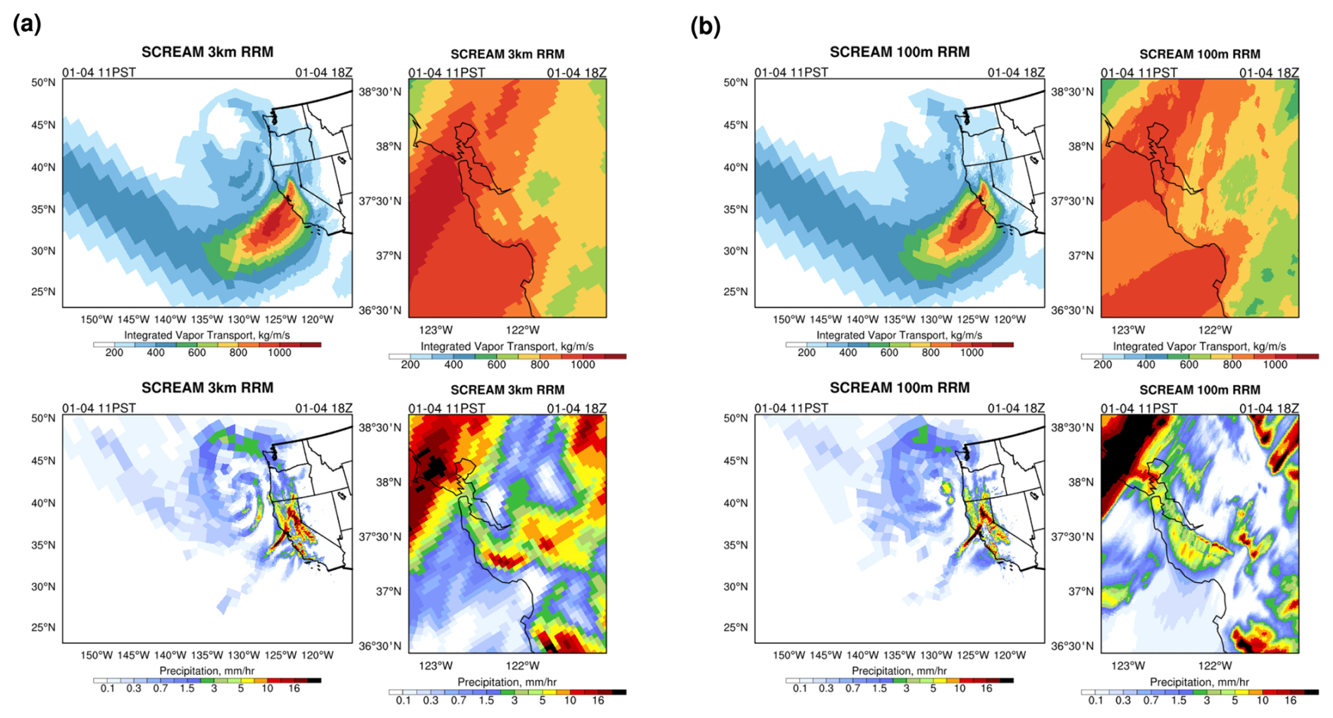
Figure 5 (a) Integrated vapor transport (top) and precipitation (bottom) in the East Pacific (left) and a zoomed-in view of the Bay Area (right) in the 3.25 km California SCREAM-RRM at 4 January 2008 18:00 Z. (b) Same as (a), but for the 100 m Bay Area SCREAM-RRM.

3.2 Stratocumulus2023

The second case, which we refer to as Stratocumulus2023, covers a weak synoptic wind condition dominated by marine stratocumulus. This case was initialized at 00:00 Z on 10 July 2023 and simulated for 48 h. It is representative of typical summer conditions, featuring marine stratocumulus clouds that form inland during the night and gradually retreat toward the coast by midday. The Central Valley experiences arid, Mediterranean-like summer conditions, which generally inhibit marine stratocumulus from penetrating far inland. However, these clouds often reach the interior valleys of the San Francisco Bay Area (e.g., Livermore). Locals often note the contrast: overcast, dewy, and cool conditions in the early morning, which recede by noon to give way to hot, clear skies. We selected this case based on the historical temperature records in Livermore and GOES-W 0.6 µm visible imagery for North America (https://satcorps.larc.nasa.gov/, last access: 25 January 2025) from 2020–2023. Concurrent NOAA observations in Redwood City recorded average wind speeds of 5–10 m s⁻¹, with gusts of comparable magnitude. The winds exhibited a pronounced diurnal cycle. Under weak synoptic forcing, topography and boundary-layer turbulence strongly modulate the flow. Figure 6 shows liquid water path and cloud fraction of the coastal stratocumulus near San Francisco at 11 July 2023 18:00 Z simulated by both versions of SCREAM-RRM. Since there is no data for this day from North America GOES-W, we compare to the GOES-East/West Merged CONUS LWP-Best Estimate.

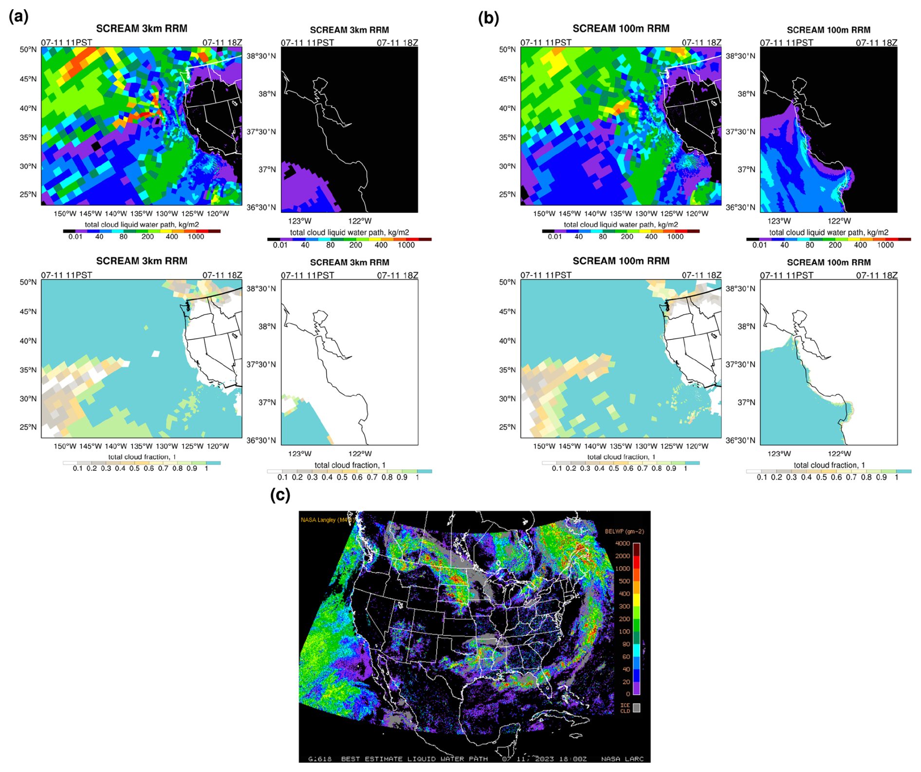
Figure 6 (a, b) Similar to Fig. 5, but for total cloud liquid water path (top) and total cloud fraction (bottom). (c) GOES-East/West Merged CONUS LWP-Best Estimate for North America.

4 Results

We begin the results section with a visual overview of the SCREAM 100 m Bay Area RRM (referred to as “BA-100m”) simulated vertical motion and cross sections. These high-resolution snapshots highlight the 100 m RRM's ability to resolve fine-scale processes such as topography-induced lifting, boundary-layer structure, and wave activity. A particularly notable feature is the presence of high-frequency wind speed oscillations, which closely resemble those seen in observations.

We then conduct a more detailed evaluation of the performance of BA-100 m and the SCREAM 3.25 km CA RRM (referred to as “CA-3 km”) under two contrasting weather regimes: the synoptically forced Storm2008 case and the locally driven Stratocumulus2023 case. Specifically, we calculated the metrics of these simulations to in-situ observations of near-surface temperature, wind speed, relative humidity, and surface pressure. The spatial distribution of these variables is generally smooth across a few hundred meters, so direct comparison with station data is feasible for the 100 m and 3.25 km RRMs. In addition to the overall skill scores, we particularly emphasize SCREAM's ability to capture the temporal evolution of meteorological factors at each site, especially by utilizing the 6 min high-frequency observation data from Tides and Currents. Furthermore, we compare the sounding data at Oakland International Airport station, focusing on the differences in temperature and humidity in the boundary layer.

4.1 An initial look at the 100 m SCREAM-RRM runs

Videos A1 and A2 (Zhang, 2026, https://doi.org/10.5446/s_1996) show the evolution of vertical velocity (w) and precipitation at upper (332 hPa), lower-middle (808 hPa), and boundary layer (951 hPa) levels in the BA-100 m and CA-3 km simulations. Each frame represents a 10 min interval, capturing the temporal progression of atmospheric features at high resolution.

BA-100 m shows remarkable detail (see Video A1 in Zhang, 2026; Fig. 7). One question is how much of this rich detail is realistic? Accurate observations of w, gravity waves, and precipitation are notoriously difficult, making it hard to directly assess the objective full picture of the “true value”. However, these videos and images serve as a reminder of several fundamental characteristics of fluid dynamics.

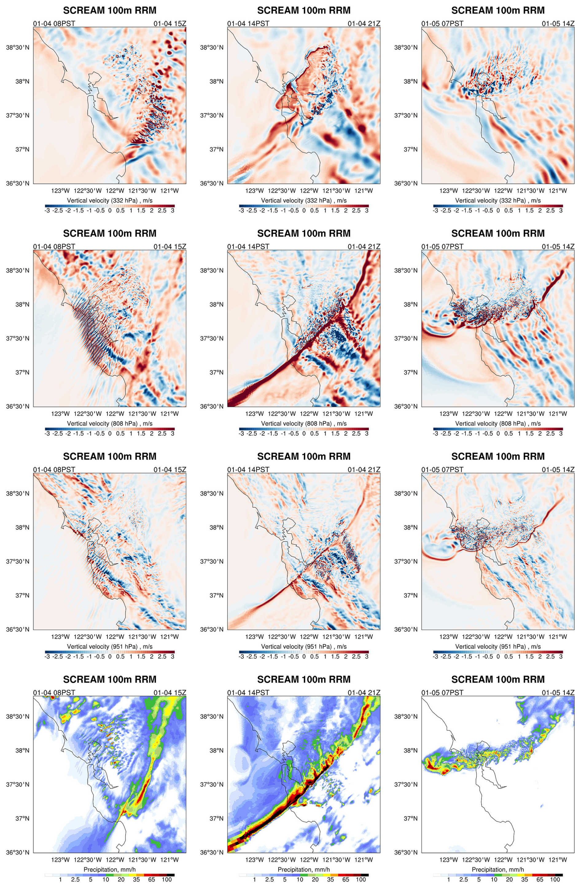
Figure 7 Vertical velocity at 332 hPa (top row), 808 hPa (second row), and 951 hPa (third row), along with the total precipitation rate at the surface (bottom row), at 4 January 2008 08:00 PST (left), 4 January 2008 14:00 PST (middle), and 5 January 2008 07:00 PST (right), in the 100 m Bay Area SCREAM-RRM simulation.

In the Storm2008 case, several distinct features emerge. First, a persistent, mountain-scale standing wave pattern is present throughout the simulation, with its wavelength increasing with altitude. Second, strong updrafts develop ahead of the cold front as high-speed winds interact with the coastal topography, generating substantial turbulence and wave instabilities – both convective and shear-driven – in the downstream region. Third, a vortex forms over the ocean and intensifies as it approaches the coast. Upon colliding with the Marin Hills, the vortex undergoes deformation and nonlinear fragmentation, further enhancing local turbulence. Just before landfall, it induces strong divergence and subsidence through evaporative cooling, producing a well-defined cold pool and gust front. During the final third of the simulation, multiple suspected cold pools propagate successively inland. Their gust fronts are evident in the 850 hPa w field. We recommend readers consult the animations in Video Supplement, which contains far more information than can be captured in static snapshots.

While the meticulous depiction of these features and their phenomenological plausibility is encouraging, it does not necessarily validate the intensity of the perturbations. Due to the lack of direct observations, quantifying the realism of these perturbations in each local region remains difficult. However, available routine observations provide some insights (see next section). For instance, while the simulated cold pool characteristics align with the simulated temperature decrease and pressure increase over the last 12 h, no such signal is evident in the observations, raising questions about the validity of this specific process. The encouraging aspect is that no obviously suspicious numerical artifacts were detected.

Stratocumulus2023 provides a more intuitive example, demonstrating the seamless transition of the RRM grid across different scales without spurious fluctuations at the boundaries (see Video A2 in Zhang, 2026; Fig. 8). The vertical motion of the boundary layer exhibits a pronounced diurnal variation. After sunrise, as the surface heats up, the boundary layer deepens, where the turbulence intensifies substantially compared to nighttime. The horizontal half-wavelength of fluctuations in the 100 m refinement region is about 1 km, corresponding roughly to SCREAM's effective resolution of about 6Δx (600 m) (Caldwell et al., 2021). The transition from the 100 m refinement region to the 800 m refinement region is rapid, with the wavelength increasing to about 10 km. This transition appears natural and does not introduce numerical artifacts. Similarly, the transition from the ocean to the coastal ranges due to topography leads to a wavelength shift from greater than 10–1 km, also appearing physically plausible. During the first night of the simulation, stratocumulus is developing near the San Francisco coast (Video A2 in Zhang, 2026).

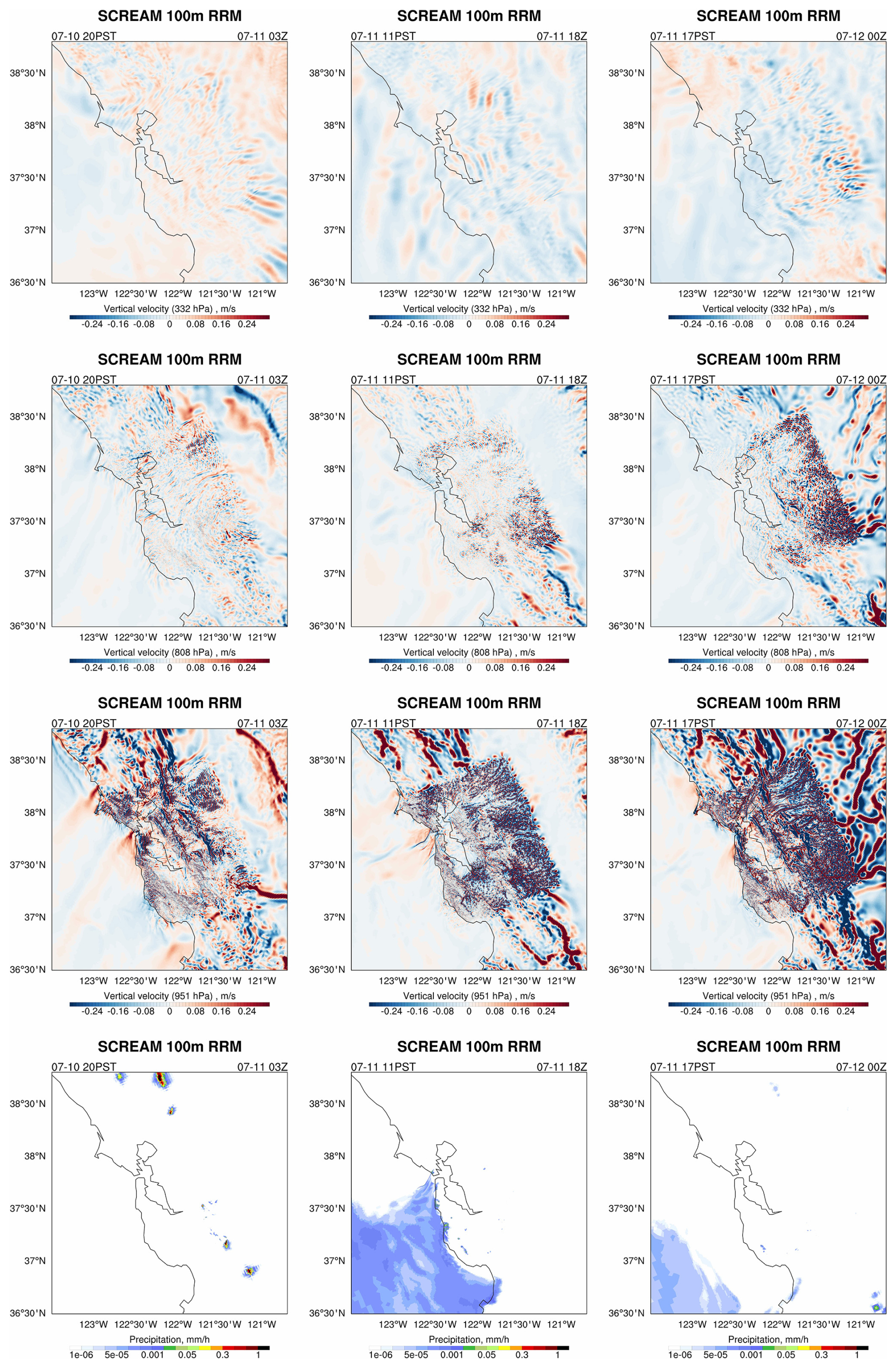
Figure 8 Same as Fig. 7 but for the Stratocumulus2023 event at 10 July 2023 20:00 PST (left), 11 July 2023 11:00 PST (middle), and 11 July 2023 17:00 PST (right).

Cross sections provide additional insight into the small-scale vertical structures captured by the 100 m simulation. In Storm2008, strong updraft zones emerge across the coastal ranges and extend deep into the troposphere (Fig. 9a). While cloud formation generally aligns with areas of upward motion, the strongest clouds do not always coincide with the most intense updrafts, likely reflecting the influence of horizontal advection of condensate and drag effects from falling precipitation. Additionally, a pair of oppositely rotating horizontal vortices is evident: one at mid-levels downstream of the frontal zone and another farther downstream in the lower troposphere. This suggests the presence of both convective and shear-driven instabilities (e.g., Sun et al., 2015). The 3.25 km simulation exhibits far less detail in the vortex structures, hydrometeor distribution, and updraft features compared to the 100 m simulation in the frontal region. In contrast, Stratocumulus2023 is characterized by weaker topographic forcing and more thermally driven turbulence (Fig. 9b). The short horizontal wavelengths of boundary-layer fluctuations remain intact to mid-levels, with limited vertical propagation due to weak ambient wind. These results demonstrate that SCREAM-BA-100 m physically represents complex vertical transport and wave dynamics across different flow regimes.

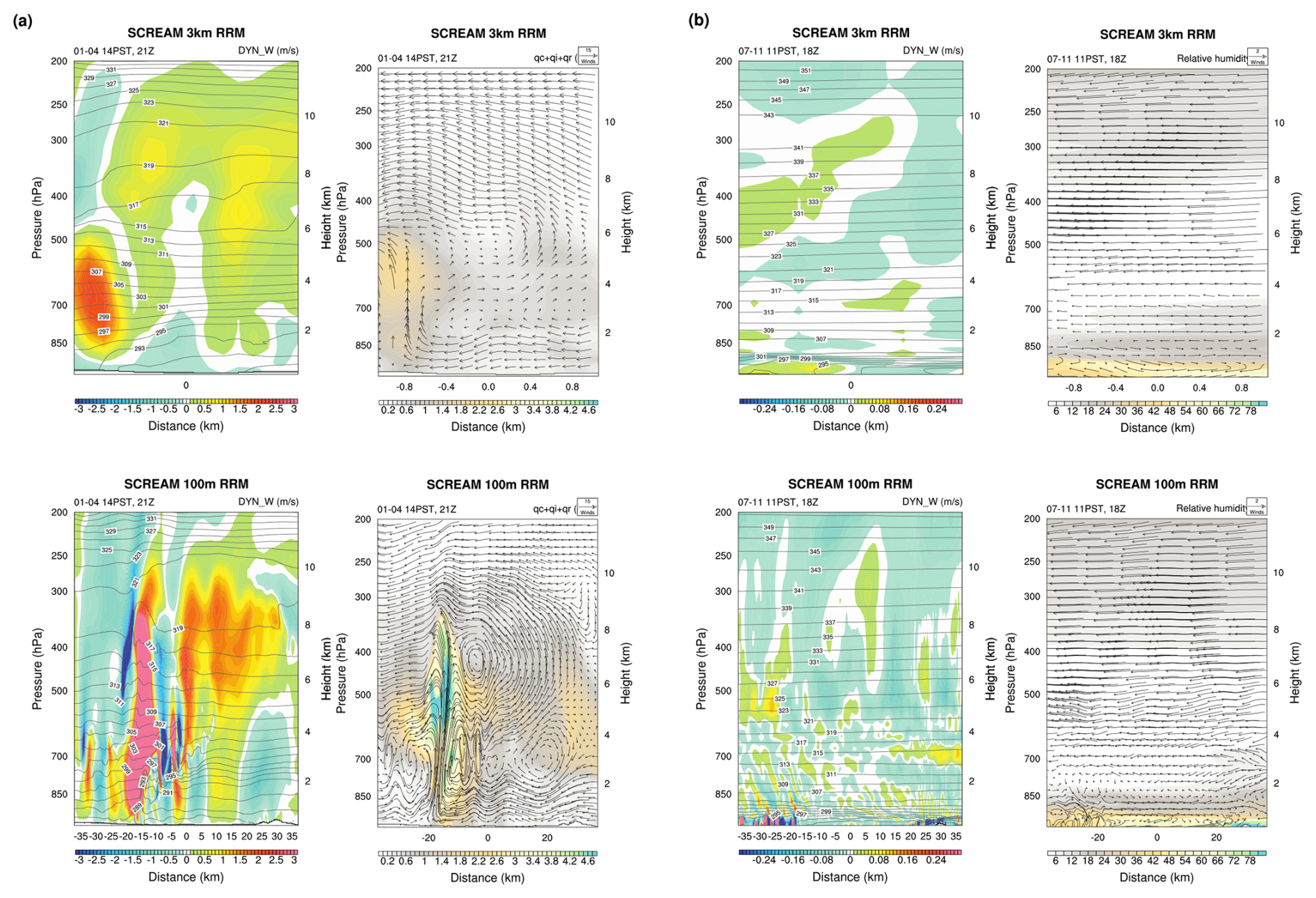
Figure 9 Cross sections (a) the Storm2008 event (4 January 2008 14:00 PST) and (b) the Stratocumulus2023 event (11 July 2023 11:00 PST) aligned parallel to the Santa Cruz Mountains extend from the southeast (238° E, 37.3° N) to the northwest (237.5° E, 37.8° N), spanning 74 km along the x axis. The cross-section line is shown in orange-red in Fig. 4 on the IGRA station map. Each panel shows vertical velocity (shading) overlaid with potential temperature (contours) on the left, and total cloud hydrometeors (liquid + ice + rain) overlaid with wind vectors on the right, from the 3.25 km California (top) and the 100 m Bay Area (bottom) SCREAM-RRM simulations. Horizontal winds are adjusted to be parallel to the cross-section, and vertical velocity is amplified by a factor of 10.

4.2 In-situ evaluation

4.2.1 Storm2008

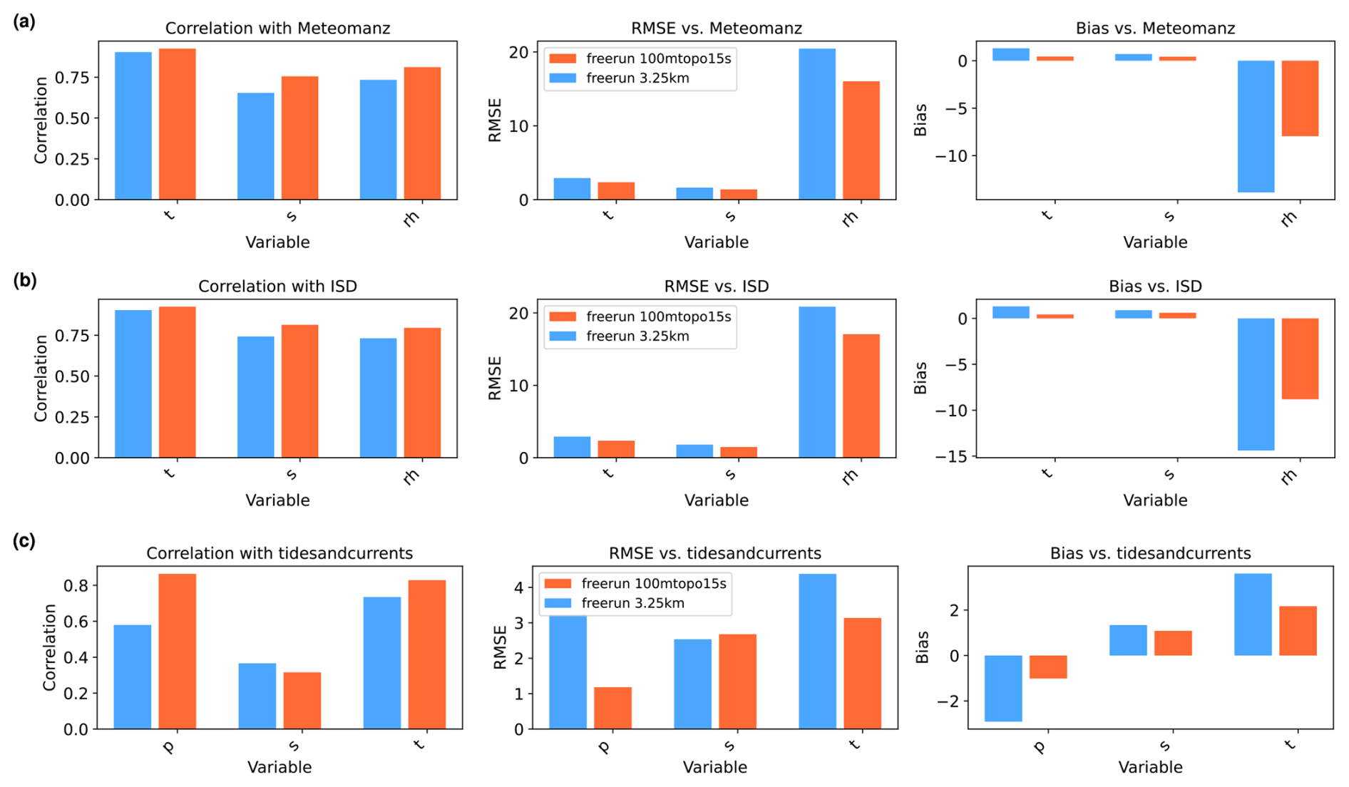
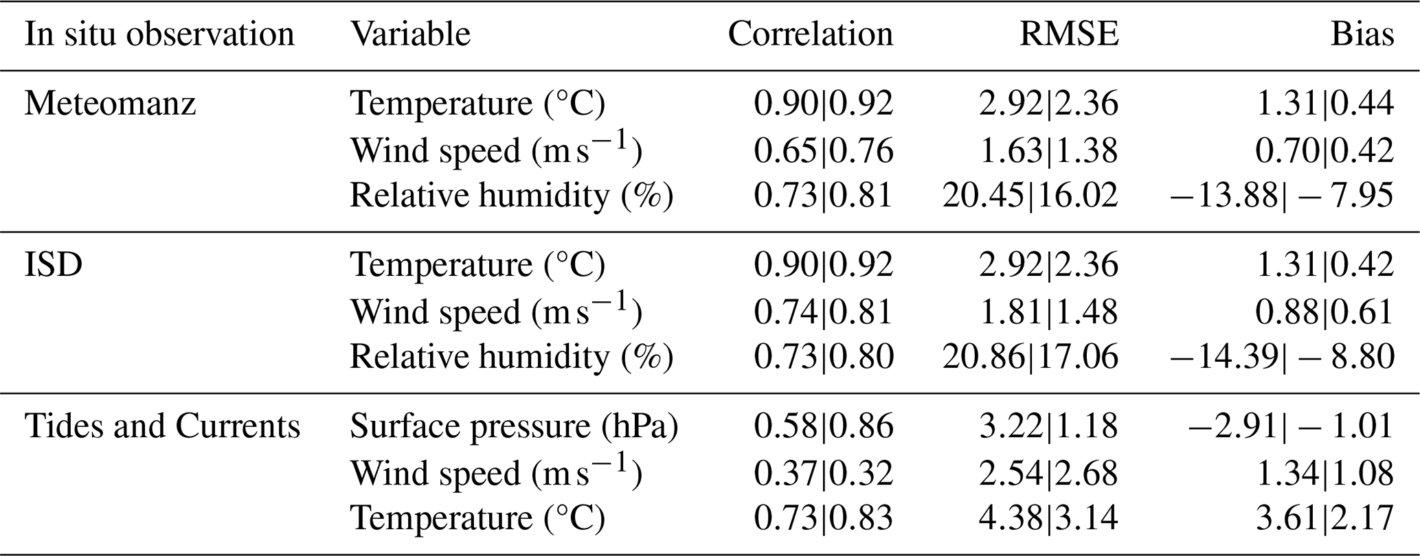
Figure 10 and Table 1 present the overall skill scores including correlation coefficients, root mean square errors (RMSE), and biases for near-surface temperature, wind speed, relative humidity, and surface pressure from the SCREAM-RRM simulations of the Storm2008 event. These metrics are evaluated against observations from Meteomanz, ISD, and Tides and Currents stations, all of which are located within the 100 m rectangular domain shown in Fig. 4. Among these sources, Meteomanz provides data from only two stations, whereas Tides and Currents offers the most extensive coverage. The RMSE and bias for all variables show substantial improvement in the BA-100 m simulation compared to CA-3 km. In terms of correlation, temperature exhibits a decrease in BA-100 m, while relative humidity shows an increase. Wind speed correlations decrease (increase) relative to Tides and Currents (Meteomanz and ISD) observations, and surface pressure shows a modest reduction in correlation when evaluated against Tides and Currents data.

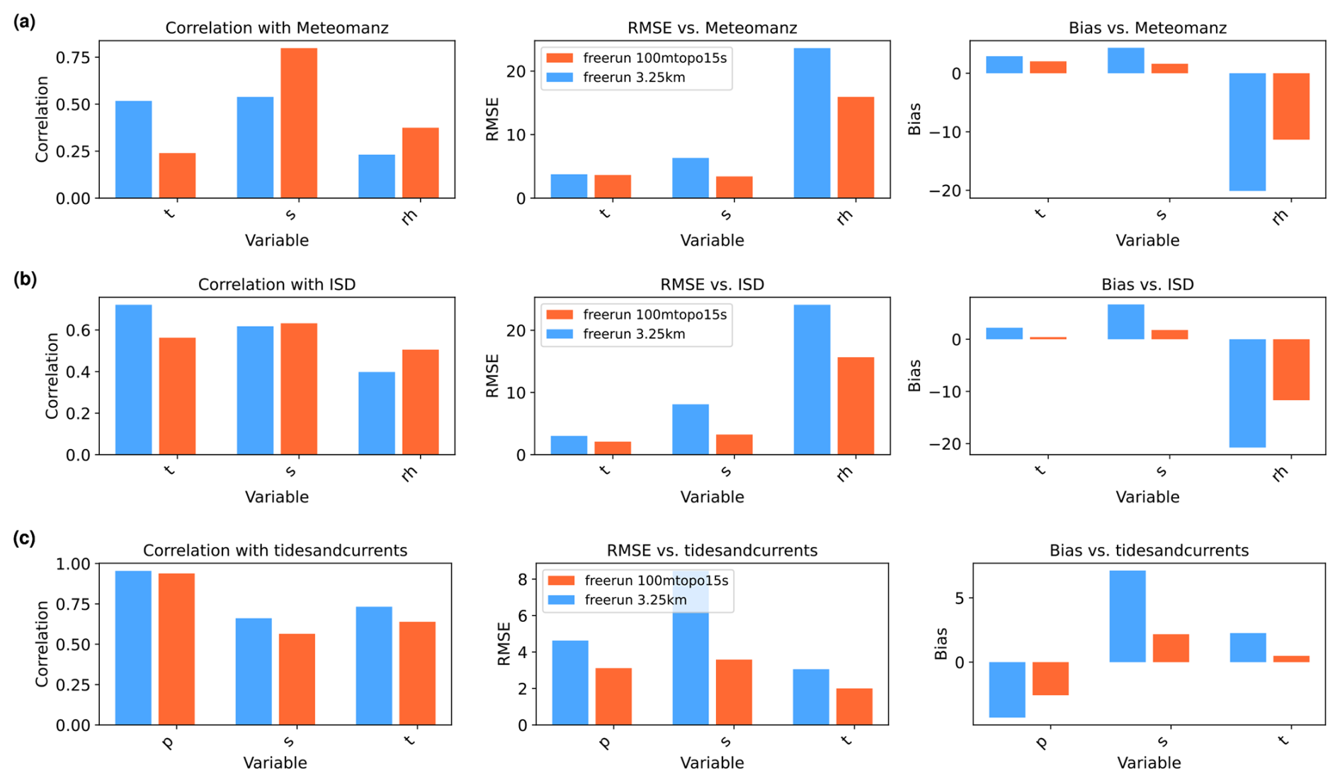
Figure 10 Skill scores for the Storm2008 event are shown for near-surface temperature (t), wind speed (s), relative humidity (rh), and surface pressure (p). These are compared against observations from (a) Meteomanz, (b) ISD, and (c) Tides and Currents, and presented as three overall metrics: Pearson correlation coefficient (left), root-mean-square error (RMSE, middle), and bias (right). The blue and orangered bars indicate simulation results from the 3.25 km California SCREAM-RRM and the 100 m Bay Area SCREAM-RRM, respectively.

Table 1 Skill metrics for the Storm2008 event are shown for near-surface temperature, wind speed, relative humidity, and surface pressure compared to Meteomanz, ISD, and Tides and Currents in situ observations. Metrics include Pearson correlation coefficient, RMSE, and bias. For each variable, values are shown for the 3.25 km California SCREAM-RRM and the 100 m Bay Area SCREAM-RRM simulations, separated by a vertical bar (3.25 km|100 m).

Ten ensemble members were run for CA-3 km to assess sensitivity to initial condition perturbations. We checked the standard deviation across ensemble members, which shows that the relatively large bias and RMSE persist, highlighting the key role of resolution sensitivity rather than random variability. Ensemble spread appears after hour 34 of the simulation, most prominently in wind speed and relative humidity, but does not alter the first-order comparisons with observations or BA-100 m. Spatially, except for small uncertainty in the location of the precipitation maximum, the moisture transport and precipitation patterns are highly robust (not shown).

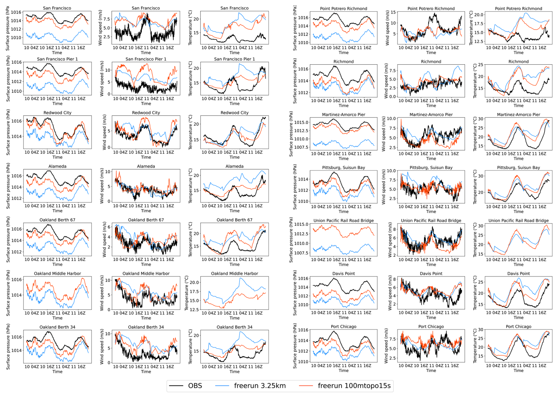
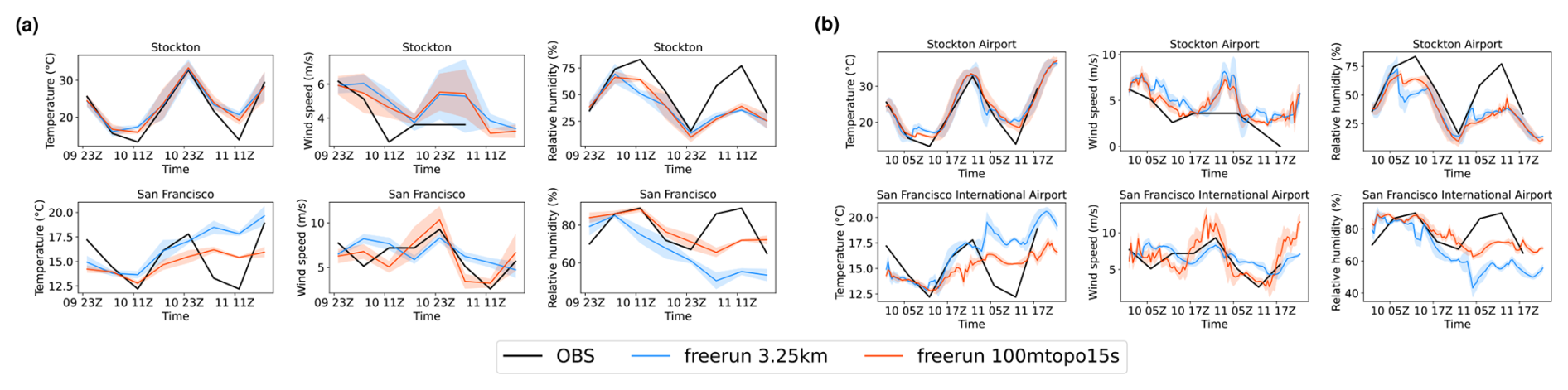
A more intuitive understanding can be gained from the detailed temporal evolution of each station (Figs. 11 and 12). Observations show a notable drop in air pressure, wind speed, and temperature after the cold front passage. Temperature observations at multiple stations exhibit a roughly four-hour period of rising followed by falling values. The previous evolutions shown in Video A1 in Zhang (2026) suggest this behavior may be associated with weak pre-frontal convergence in the region. Compared to the observations, CA-3 km exhibits a warm bias, a high wind speed bias, a dry bias, and a lower air pressure bias. BA-100 m compares better with the observations for all variables, reducing all biases. Note that Stockton station is located just outside the 100 m domain, so a comparatively modest improvement there is expected.

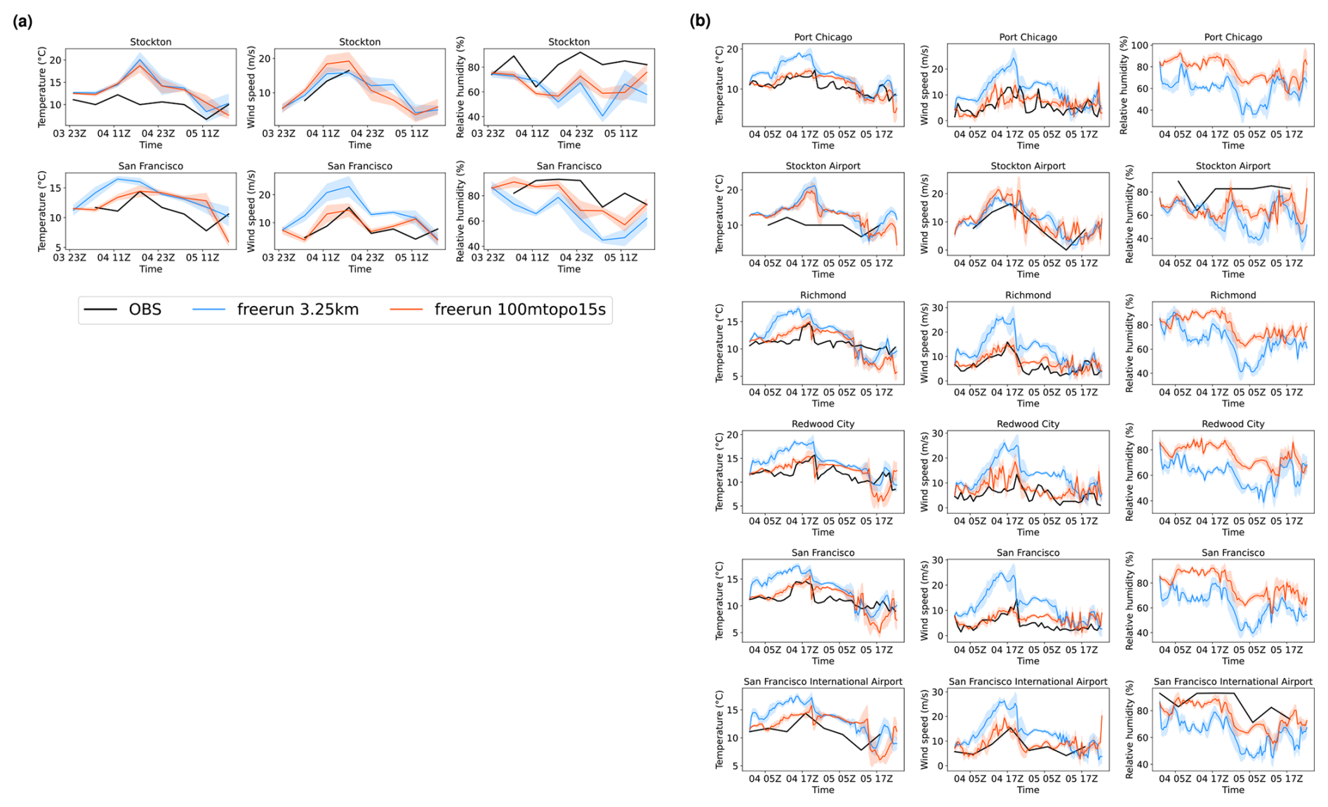
Figure 11 (a) Time series at each station for the Storm2008 event, with black, blue, and orangered lines representing Meteomanz observations, the 3.25 km California SCREAM-RRM simulation, and the 100 m Bay Area SCREAM-RRM simulation, respectively. (b) Same as (a), but for ISD observations. From left to right, the columns show near-surface air temperature, wind speed, and relative humidity. The bold line shows model output resampled from 5 min resolution to match the observational intervals as instantaneous values; shading denotes the standard deviation within each observational window.

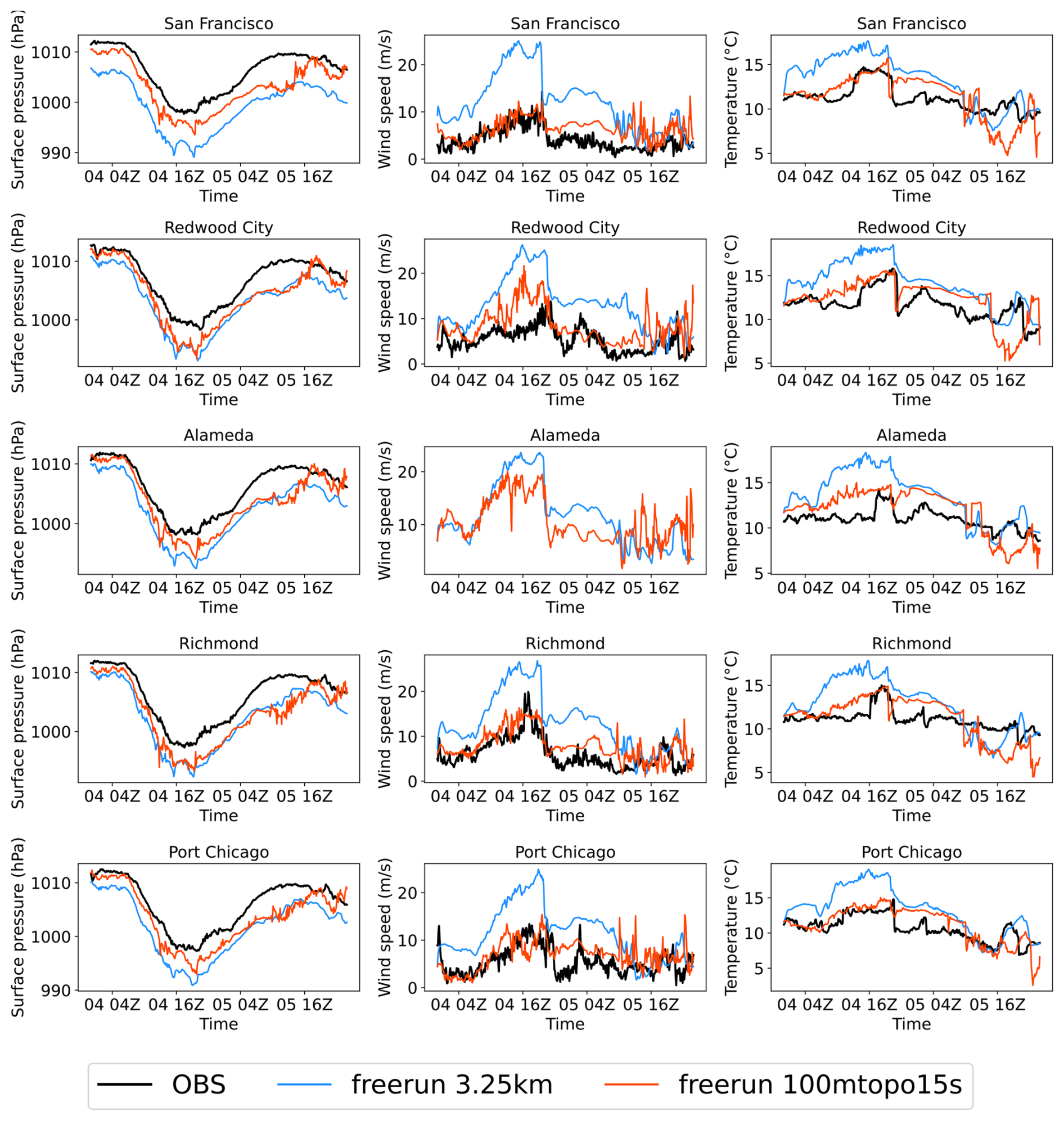
Figure 12 Same as Fig. 11 but for Tides and Currents observations. From left to right, the columns show surface pressure, wind speed, and near-surface air temperature.

Despite the overall improvements, BA-100 m still exhibits biases in simulated surface pressure, relative humidity, and temperature on the second day. Notably, it fails to capture the observed four-hour temperature rise preceding the cold front. In the latter half of the day, the simulated temperature phase diverges markedly from observations, likely reflecting the reduced predictability of this bomb cyclone under free-running simulation conditions.

The improvement in wind speed simulation with BA-100 m is particularly noteworthy. Aside from a spurious peak occurring after the 36th simulation hour which is absent in observations, the enhanced performance persists throughout most of the period. Furthermore, the model captures high-frequency wind speed oscillations that align well with Tides and Currents observations, suggesting a realistic representation of small-scale gravity wave activity. However, BA-100 m overestimates wind speeds at Redwood City during the first day's daytime hours and underestimates the post-frontal wind speed reduction, particularly at the Port Chicago station.

A comparison with sounding observations from Oakland International Airport at the model initialization time reveals a notable bias introduced by the ERA5 initial conditions (Fig. 13). While upper-level comparisons are less reliable due to increasing temporal mismatch as the pilot balloon ascends and potential trajectory shifts under strong synoptic winds, substantial deviations are evident below 700 hPa. Specifically, the dew point is up to 3 K lower below 900 hPa and up to 3 K higher above that level, while temperatures in the boundary layer are consistently 1–2 K higher than observed.

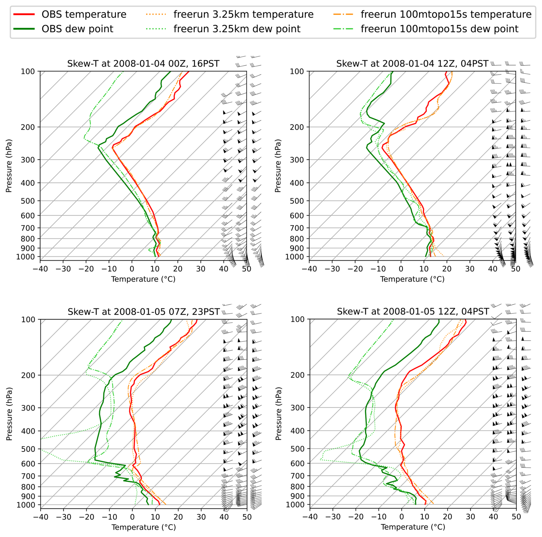
Figure 13 Soundings at Oakland International Airport for the Storm2008 event. Red and green lines represent air temperature and dew point from IGRA observations (thick solid), the 3.25 km California RRM (semi-transparent dotted), and the 100 m Bay Area RRM (semi-transparent dotted-dashed), respectively. From left to right, the wind barbs correspond to IGRA observations, the 3.25 km simulation, and the 100 m simulation.

The dew point and temperature biases in the initial conditions are consistent with those identified in the station-based evaluation, suggesting that some of the persistent warm and dry biases in SCREAM originate from the ERA5 initial conditions. In the CA-3 km simulation, a clear trade-off between dry and warm biases emerges: when the dry bias is more pronounced, the warm bias tends to be reduced (e.g., 5 January 07:00 and 12:00 Z), and vice versa (e.g., 4 January 12:00 Z). In contrast, the BA-100 m simulation exhibits a substantial reduction in the dry dew point bias below 900 hPa, particularly near the surface and most notably during the second night. As the simulation progresses, differences between CA-3 km and BA-100 m become more pronounced at all vertical levels, with BA-100 m generally aligning more closely with observations, except for a warm temperature bias at 12:00 Z on the second day.

Estimated planetary boundary layer height (PBLH) at Oakland International Airport using a RH-gradient method agrees closely between CA-3 km and IGRA, with differences that are visually indistinguishable. The BA-100 m simulation generally underestimates PBLH.

In addition, CA-3 km shows a pronounced wind speed overestimation near 800 hPa. As the simulation progresses, wind differences between BA-100 m and CA-3 km increase, with BA-100 m more closely matching observations throughout the lower to mid-troposphere (Fig. 13). By 12:00 Z on the second day, CA-3 km exhibits a near-surface wind direction error of almost 90°, while BA-100 m remains largely aligned with the observations.

In the Storm2008 case, the BA-100 m simulation markedly reduces the high wind speed bias as well as the warm and dry biases of the 3.25 km simulation. These improvements likely arise from finer resolution of TKE and more effective turbulent mixing, as well as potential feedbacks from precipitation processes, given that BA-100 m can capture much shorter wavelengths (see Sect. 4.4) and more accurately align precipitation with local orographic features in complex terrain (see Fig. 7 and Video A1). The improved wind speed simulation may also contribute to reductions in temperature and humidity biases, as weaker near-surface winds allow for the localized accumulation of cooler, moister air masses associated with evaporative cooling from precipitation. The remaining warm and dry biases are likely influenced, at least in part, by inaccuracies in the initial conditions (Figs. 13 and 17) – a plausible outcome given the 31 km native resolution of the ERA5 reanalysis. Furthermore, San Francisco Bay and San Pablo Bay are treated as ocean grid points in the model, with surface temperatures prescribed by 1° SST data. This coarse representation fails to capture the actual temperature distribution near adjacent stations and represents an additional source of bias beyond the initial conditions.

4.2.2 Stratocumulus2023

Figure 14 and Table 2 present the overall skill scores for near-surface temperature, wind speed, relative humidity, and surface pressure for the Stratocumulus2023 event. Under the locally driven flow conditions of Stratocumulus2023, the CA-3 km simulation exhibits substantially lower RMSE and bias in wind speed and surface pressure compared to the Storm2008 case. The BA-100 m simulation demonstrates an overall reduction in RMSE and bias for all variables and all datasets. Correlation coefficients also improve for most variables in BA-100 m, with the exception of wind speed, which exhibits a reduced correlation with Meteomanz and Tides and Currents. The CA-3 km ensemble shows virtually no ensemble spread throughout the two-day simulation.

Figure 14 Same as Fig. 10 but for the Stratocumulus2023 event.

Table 2 Same as Table 1 but for the Stratocumulus2023 event.

A detailed station-by-station comparison with Tides and Currents observations (Fig. 15) reveals that while wind speed performance in BA-100 m degrades at a few stations, such as San Francisco Pier 1 and Port Chicago, most stations exhibit notable improvements relative to CA-3 km. The frequency of wind speed oscillations in BA-100 m more closely matches observations, although the simulated oscillations are less pronounced and less continuous than those observed. Surface pressure bias is also substantially reduced in BA-100 m, typically decreasing from approximately 3 to below 1 hPa.

Figure 15 Same as Fig. 12 but for the Stratocumulus2023 event.

Figure 16 Same as Fig. 11 but for the Stratocumulus2023 event.

The CA-3 km simulation exhibits an unrealistic temperature jump during the 4th hour of the simulation, characterized by an initial cooling followed by rapid warming – a feature consistently reflected across all Tides and Currents stations. This behavior may be associated with mesoscale wave responses triggered by the coarse representation of topography. The artificial temperature jump is followed by a sustained warm bias in CA-3 km, reaching 2–4 K during the first day. On the second day, this bias becomes more pronounced, with some sites exhibiting temperature overestimations of up to 8 K. In contrast, the BA-100 m simulation maintains a temperature bias below 1 K during the first 12 h of nighttime. However, during the daytime, BA-100 m shows a more rapid and exaggerated temperature increase compared to observations, leading to an overestimation of the daytime maximum temperature. Notably, BA-100 m also develops a substantial warm bias on the second day, though it is approximately half the magnitude of that in CA-3 km.

This behavior is likely linked to the simulation of coastal stratocumulus west of San Francisco, as illustrated in Fig. 6. The CA-3 km simulation fails to reproduce coastal stratocumulus on the second day, whereas BA-100 m captures the feature, albeit with a smaller spatial extent than indicated by satellite observations and with a faster inland retreat. This improved representation is consistent with enhanced relative humidity in San Francisco, as observed in the Meteomanz and ISD data (Fig. 16).

Comparison with IGRA sounding observations shows that near-surface wind shear is well captured in CA-100 m, except for a slight underestimation in Storm2008 on 5 January 23:00 PST (Fig. 13) and Stratocumulus2023 on 11 July 05:00 PDT (Fig. 17). Mirocha et al. (2010) found that an aspect ratio between 2 and 4 yielded the best agreement with similarity solutions in their boundary-layer LES simulations using WRF. The near-surface aspect ratio in SCREAM falls within this range.

Unlike Storm2008, the initial conditions of Stratocumulus2023 show much better agreement with IGRA sounding observations (Fig. 17). This improved alignment is partly due to the calm weather and slowly evolving synoptic pattern, which limits the horizontal drift of the balloon, even at higher altitudes. Nevertheless, some discrepancies remain. Distinct peaks in dew point and temperature are evident in the IGRA soundings at specific pressure levels (e.g., 940, 750 and 500 hPa), but these features are absent in the model initial conditions, which appear considerably smoother. This mismatch is likely attributable to the limited vertical resolution in both the IFS model used to generate ERA5 and in SCREAM itself.

Figure 17 Same as Fig. 13 but for the Stratocumulus2023 event.

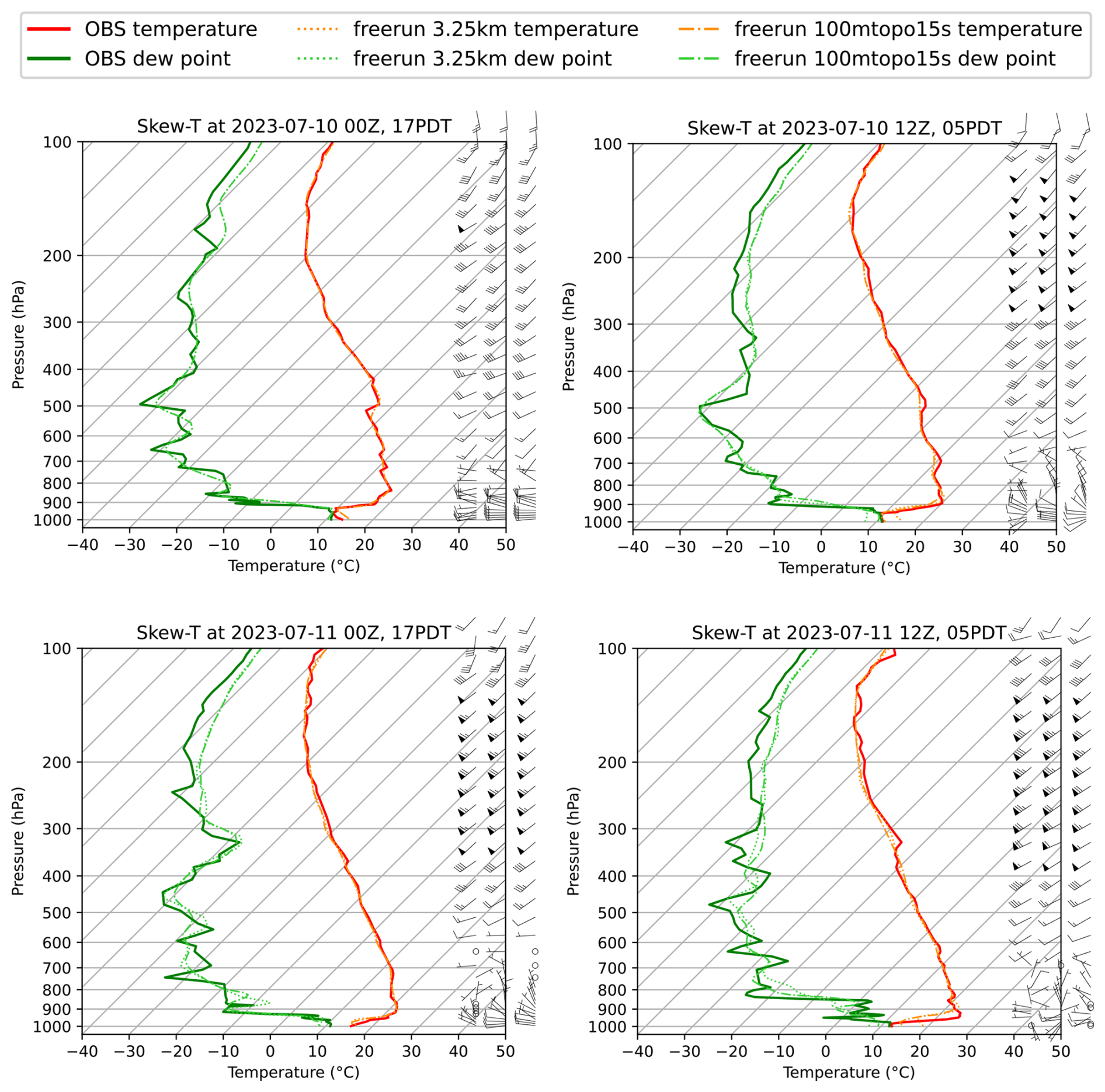
At the Oakland International Airport station, the model initial condition shows a dew point bias within 1 K below 950 hPa near the surface, while the temperature is 1–2 K higher than observed. This is consistent with the warm bias at initialization time reported in the Tides and Currents data from Oakland Berth 67/Berth 34. The difference between CA-3 km and BA-100 m grows modestly over time but remains substantially smaller than the disparity observed in the Storm2008 case. Below 500 hPa, BA-100 m aligns more closely with observations, particularly during the second night (11 July 12:00 Z). The dew point decreases more sharply from the surface to approximately 850–800 hPa, although the gradient is still less pronounced than in the observed profile.

From the top of the boundary layer to near the surface, BA-100 m shows markedly improved agreement with observations during the nighttime, with minimal temperature and dew point biases at 10 July 12:00 Z (Fig. 17). By 11 July 12:00 Z, a modest bias develops, with the dew point 2 K lower and the temperature 2 K higher than observed. In contrast, the CA-3 km simulation exhibits a dew point bias 2–3 K larger than that in BA-100 m, along with a warm bias of approximately 4 K. We note that the estimated PBLH using a RH-gradient method from BA-100 m aligns better with IGRA, while CA-3 km tends to overestimate the stratocumulus boundary layer height.

We speculate that the improved performance in this locally driven flow regime primarily results from enhanced representation of turbulent mixing (see Sect. 4.3). The observed daytime warming and wind speed increase on the first day suggest that continental heating may be overestimated. It remains unclear to what extent this bias arises from the radiation scheme, which does not currently incorporate topographic shading or surface reflections. Additionally, the sea surface temperature along the San Francisco coastline may be insufficiently resolved, contributing further to the discrepancies.

Despite improvements, the model consistently underestimates surface pressure at the majority of stations. It remains unclear whether this bias is related to model dynamics. One possible factor tied to the initial conditions is the surface adjustment procedure, which assumes a dry adiabatic lapse rate. Some groups have begun blending reanalysis data at O(10) km resolution with k-scale analysis products to initialize k-scale models. An alternative view suggests that, while mesoscale kinetic energy is initially lacking, it can rapidly spin up (Skamarock, 2004), so supplying only large-scale energy may not result in significant degradation.

In summary, our findings reinforce the scale awareness previously demonstrated in DP-SCREAM and highlight SCREAM's strong performance at LES resolution, particularly when coupled with realistic topography and surface heterogeneity.

4.3 Sub-grid-scale flux

Building on the resolution sensitivity study of DP-SCREAM in Bogenschutz et al. (2023), SCREAM exhibits characteristics of a scale aware model. As horizontal resolution increases, the partitioning between SGS and resolved turbulence diminishes. This scale awareness, inherent to the SHOC parameterization (Bogenschutz and Krueger, 2013), enables SCREAM to operate effectively at 100 m resolution without the need for parameter tuning. Specifically, Figs. 9 and 16 in Bogenschutz et al. (2023) show that in the marine stratocumulus case, maritime shallow cumulus case, and mixed-phase Arctic stratocumulus case, as the horizontal grid spacing Δx decreases, the contribution of SGS moisture flux becomes smaller while the resolved flux becomes increasingly dominant. In the 100 m DP-SCREAM simulations, above 0.2 km, the proportion of SGS moisture flux is negligible, and the resolved flux is nearly unity.

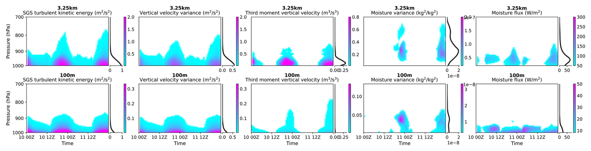
In our simulations, although we did not output high-frequency resolved moisture flux or TKE, Figs. 18 and 19 shows substantial reductions in SGS TKE, moisture flux/variance, w variance, and the third moment of w in the BA-100 m simulations compared to the CA-3 km simulations. For clarity, the plotted ranges in these figures differ between the two resolutions, with the CA-3 km values being much larger.

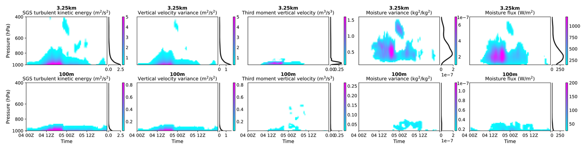
Figure 18 Simulated Sub-grid-scale (SGS) variables in the 3.25 km California RRM (top) and 100 m Bay Area RRM (bottom) during the Storm2008 event. From left to right: TKE, vertical velocity variance, third-moment vertical velocity, moisture variance, and moisture flux. Each panel consists of a time–evolution shading plot on the left and a vertical profile averaged over the simulation period on the right. For clarity, the colorbars differ between the 3.25 km and 100 m simulations, with the former being much larger.

Figure 19 Same as Fig. 18 but for the Stratocumulus2023 event.

At 100 m resolution, simulations are close to, but largely below, the turbulence gray zone, where the grid spacing becomes comparable to the dominant eddy scale. The gray zone typically spans the transition from mesoscale models, which rely on ensemble-averaged vertical fluxes, to LES, where most turbulent motions are explicitly resolved and subgrid closures play only a minor dissipative role (Wyngaard, 2004). In this transitional regime, subgrid transport is best treated with 3D turbulence schemes that represent the full stress tensor (e.g., Wyngaard, 2004; Chow et al., 2019; Honnert et al., 2020), whereas SHOC currently parameterizes only vertical mixing. Thus, at coarser resolutions such as 800 m, a 3D implementation of SHOC would likely be beneficial. At 100 m, near the lower edge of the gray zone, the need for 3D turbulence remains uncertain and case-dependent, pending the implementation and testing of such a scheme in SCREAM.

Beyond the overall reduction in SGS fluxes at finer resolution, the vertical structure of moisture transport differs markedly between the two resolutions. Although the resolved moisture flux was not archived and therefore the total flux cannot be evaluated directly, the contrasting SGS-flux maxima provide insight into the nature of vertical mixing.

In the 3.25 km simulation, the maximum SGS moisture flux is located above the surface, indicating that most of the vertical moisture transport is handled by the turbulence parameterization and likely reflects bulk-like mixing in the PBL. In contrast, the 100 m simulation has the SGS moisture-flux maximum near the surface, hinting that most of the flux is resolved while the surface gradient is handled by the subgrid scheme. This interpretation is consistent with the enhanced small-scale energy in the 100 m vertical velocity spectra (Figs. 20 and 21; see Sect. 4.4), where the spectral peak is maintained across a broader range of scales before its roll-off. The stronger resolved vertical motions in the 100 m run also reach more deeply into the troposphere (also seen from the horizontal distribution in Fig. 7 and the cross section of w in Fig. 9a).

Taken together, Figs. 7, 9a, 18, and 20 tell a coherent story of how the 100 m run could more realistically distributes moisture within the atmosphere in the Storm2008 case, affecting the total precipitation amounts simulated. This highlights the model's capability in simulating turbulent motions at finer scales.

4.4 Energy spectra

Energy spectra provide a benchmark for evaluating the transition from large-scale quasi-2D motions to small-scale 3D turbulence. The canonical k⁻³ slope at synoptic scales and $k^{-\mathrm{5}/\mathrm{3}}$ slope at mesoscale wavelengths (Nastrom and Gage, 1985) are widely used to assess effective resolution and numerical diffusion in atmospheric models (e.g., Skamarock, 2004; Jablonowski and Williamson, 2011; Caldwell et al., 2021). Numerous studies have examined KE spectra in global and regional models (e.g., Bierdel et al., 2012; Skamarock et al., 2014; Durran et al., 2017; Menchaca and Durran, 2019; Prein et al., 2022; Zhang et al., 2022; Khairoutdinov et al., 2022; Silvestri et al., 2024), with some studies have emphasized the rotational and divergent components (e.g., Hamilton et al., 2008; Blažica et al., 2013; Selz et al., 2019). Spectra of vertical velocity (w) are also informative, as they emphasize divergent motions and typically peak at mesoscale wavelengths (Bryan et al., 2003; Schumann, 2019). Figures 20–21 show KE and w spectra for the Storm2008 and Stratocumulus2023 cases.

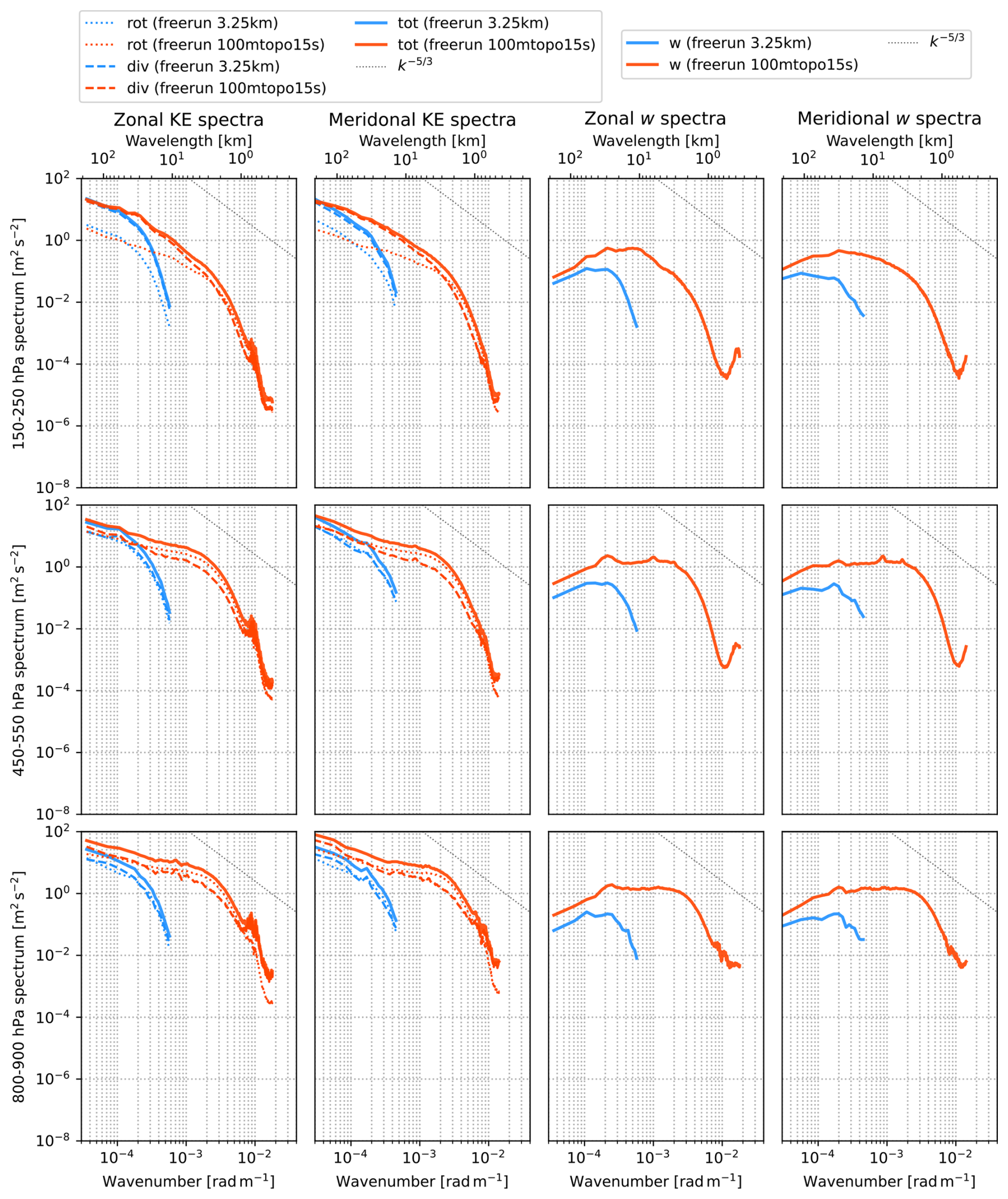
Figure 20 Energy spectra simulated by the 3.25 km California RRM (blue) and the 100 m Bay Area RRM (orangered) for the Storm2008 case. From left to right: zonal kinetic energy (KE), meridional KE, zonal vertical velocity (w), and meridional w spectra. From top to bottom: averages centered at 200, 500 and 850 hPa, each using a 100 hPa vertical window. In the KE spectra, the total, rotational, and divergent components are shown as thick solid, thin dotted, and thin dashed lines, respectively. A reference $k^{-\mathrm{5}/\mathrm{3}}$ slope line is shown in the top-right corner.

Figure 21 Same as Fig. 20 but for the Stratocumulus2023 event.

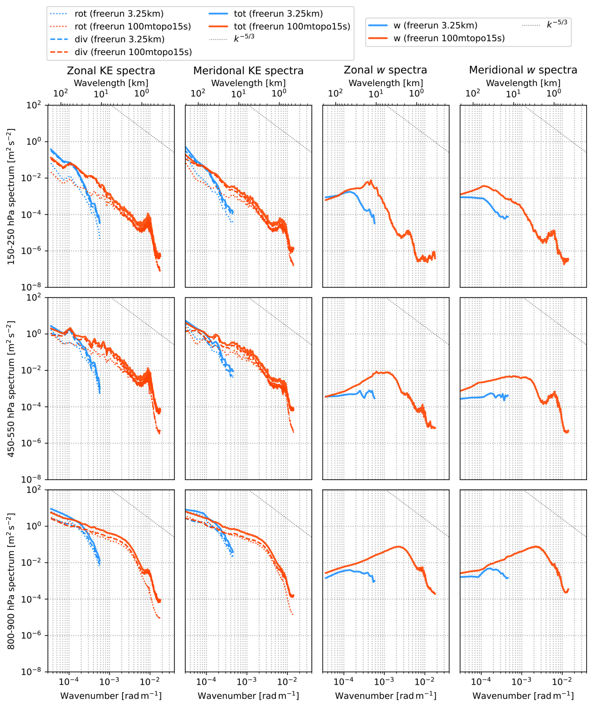
First, the CA-3 km simulations roll off sooner than the global spectra in Caldwell et al. (2021); however, we caution that the two differ in important ways (DCT over a region vs. spherical harmonics globally; two two-day events vs. 40 d statistics). For BA-100 m, the effective resolution in Stratocumulus2023 is shorter than in Storm2008 if the roll-off standard is applied. However, within the mesoscale regime (10 km–100 m), the Storm2008 KE spectra flatten relative to $k^{-\mathrm{5}/\mathrm{3}}$ before steepening again, which corresponds to the earlier roll-off. The mesoscale flattening of the KE spectra in this case may reflect a genuine accumulation of mesoscale energy, given that this was a record-breaking extreme event. In both cases, it is robust that BA-100 m contains much more small-scale energy than CA-3 km.

A notable feature in both events is a sharp KE increase between 1 km and 500 m (approximately) in BA-100 m. We suspect this results from the blocky mountain effect, caused by the mismatch between the 800 m cubed-sphere topography (the highest-resolution global dataset available) and the model's 100 m grid spacing. Toolchain memory limits prevented higher-resolution topography, so the effective topographic resolution lags behind the model Δx, producing unnaturally flat peaks and steep slopes. These slopes can generate excess high-wavenumber energy, consistent with the abrupt KE rise below 1 km. An alternative is contamination by inflow of coarser-resolution energy from the surrounding 800 m mesh via lateral boundaries. However, this is inconsistent with: (1) the effect being stronger in Stratocumulus2023 than in Storm2008, whereas boundary advection should amplify it in the latter; and (2) the 800 m mesh itself having an effective resolution of ∼4.8 km, with KE decaying rapidly beyond that, making a rise near 500 m hard to explain. To confirm the blocky mountain hypothesis, sensitivity tests with 100 m cubed-sphere topography are needed. To rule out lateral boundary effects, larger RRM domains need be tested (cf. Bogenschutz et al., 2024). In either case, toolchain memory upgrades are essential.

The w spectra exhibit a mesoscale peak, consistent with Bryan et al. (2003) and Schumann (2019), with a cutoff near 1–3 km in BA-100 m. Below 1 km, the ratio of w to KE spectra approaches unity in Storm2008 but remains below one in Stratocumulus2023, except in the lower troposphere. The temporal evolution further shows rapid development of small- and mesoscale w spectra, which are well developed within the first simulation hour (not shown).

Overall, KE spectra vary substantially across these two events, reflecting the influence of different forcing mechanisms and dynamical regimes. This aligns with Menchaca and Durran (2019) and Selz et al. (2019), and does not support a universal mesoscale KE spectrum.

5 Conclusions

This study presents the first known implementation of a global model – specifically SCREAM – at 100 m horizontal resolution within a regionally refined mesh (RRM) configuration, applied over the San Francisco Bay Area. Using two hindcast cases – one a dynamically active bomb cyclone and the other a weakly forced marine stratocumulus regime – we demonstrate that SCREAM can stably operate at large-eddy simulation (LES) scales while interacting with realistic topography, land surface heterogeneity, and coastlines. This advancement bridges the gap between idealized LES setups and full-complexity global models, offering new opportunities for process-level investigation at resolutions approaching turbulence-resolving scales.

The 100 m SCREAM-RRM simulation (BA-100 m) substantially reduces key near-surface biases relative to the 3.25 km SCREAM-RRM (CA-3 km), particularly for surface wind speed, temperature, relative humidity, and pressure. These improvements are especially evident in the Storm2008 case, where the high wind speed bias is mitigated and high-frequency oscillations in wind speed – consistent with observations – are captured. In the Stratocumulus2023 case, boundary-layer evolution and coastal cloud retreat are better represented, highlighting SCREAM's potential in both synoptically and locally driven flow regimes.

SCREAM's performance at 100 m resolution is enabled by the scale-aware SHOC turbulence parameterization, which transitions smoothly from kilometer to LES-scale without tuning. SHOC's dependence on subgrid turbulent kinetic energy and cloud-layer depth allows the model to appropriately reduce subgrid contributions as resolution increases, effectively resolving larger eddies. Furthermore, simulations at 100 m resolution largely bypass the turbulence gray zone, although future work may benefit from expanding SCREAM's current 1-D vertical subgrid turbulence treatment to a full 3-D stress tensor formulation.

In addition to scientific advances, this study highlights important performance considerations. On CPU-only systems such as Livermore Computing's Ruby cluster, simulations at 100 m resolution advance at roughly one simulated hour per wall-clock hour, requiring nearly a month to complete a two-day hindcast. However, performance scaling tests conducted on the GPU-accelerated SCREAMv1 (EAMxx) running on NERSC's Perlmutter system demonstrate a dramatic improvement, reducing the runtime to under two wall-clock days. This shift represents a crucial step toward making ultra-high-resolution simulations viable for broader research and applications.

Overall, this work demonstrates that SCREAM can be successfully extended to 100 m resolution within a global model framework using a regionally refined grid. This capability opens the door to simulating boundary-layer turbulence, orographic flows, coastal cloud systems, and convective processes at previously inaccessible scales in Earth system models. As observational constraints and diagnostic tools improve, future work should explore applications in wind energy siting, hydrological extremes, and complex terrain validation. Further development to improve topography preprocessing, initial condition fidelity, and numerical stability will enhance the robustness and reproducibility of LES-scale SCREAM simulations across diverse regions.