Attention-driven and multi-scale feature integrated approach for earth surface temperature data reconstruction

High-resolution observation is crucial for studying surface temperatures characterized by complex variations, particularly surface air temperatures in oceanic regions, which serve as significant indicators of sea-air coupling changes. Due to the scarcity of conventional observations of surface atmospheric temperatures in these areas, high-resolution surface atmospheric temperature data derived from satellite inversion has become the primary source of information. However, missing data resulting from factors such as the orbital spacing of polar satellites, cloud cover, sensor errors, and other disruptions poses substantial challenges to Earth Surface Temperature (EST) estimation. In this paper, we introduce ESTD-Net, a novel deep learning-based model designed for surface temperature data inpainting. ESTD-Net incorporates an enhanced multi-head context attention mechanism and a modified transformer block to capture long-range pixel dependencies, thereby improving the model's ability to focus on boundary regions. Additionally,the Stage Two employs a convolutional U-Net in an autoregressive manner to refine the coarse output from the Stage One, enhancing local spatial continuity and smoothing boundaries. In addition, we adapt two loss components – weighted reconstruction loss and gradient consistency regularization – to the specific demands of Earth surface temperature interpolation. Our ablation studies confirm that their integration significantly improves spatial consistency and accuracy, particularly in textureless regions and in maintaining physically meaningful gradients. Evaluation results demonstrate that ESTD-Net outperforms existing methods in both pixel-level accuracy and perceptual quality. Our approach offers a robust and reliable solution for restoring earth surface temperature data.

1 Introduction

Earth Surface Temperature (EST) refers to the kinetic temperature of the Earth's surface, encompassing both land and ocean regions. In oceanic areas, EST is a crucial parameter that reflects the thermodynamic interactions between the ocean surface and the atmosphere, playing a vital role in ocean-atmosphere coupling processes. According to surface energy balance (SEB) theory, the ocean surface absorbs energy from both incoming solar radiation and atmospheric long-wave radiation. This absorbed energy is redistributed through several mechanisms: (1) outgoing thermal radiation, which directly influences EST; (2) vertical heat transport via ocean mixing and conduction; (3) turbulent heat exchanges at the air-sea interface; and (4) phase changes in surface water, including evaporation and condensation. Given its importance in climate and weather systems, EST over oceanic regions is typically estimated using various observational approaches, including in situ measurements, reanalysis datasets, ocean models, and satellite remote sensing techniques (Zhou et al., 2018). Among these methods, satellite-derived measurements offer a highly efficient and accurate means of capturing global-scale EST variations, facilitating continuous monitoring of temperature fluctuations across the ocean surface. These observations are essential for understanding large-scale climate dynamics, enhancing numerical weather prediction, and supporting oceanographic and meteorological research.

Cloud cover presents a significant challenge in obtaining accurate EST data over oceanic regions, as it consistently obscures more than 55 % of the Earth's surface (King et al., 2013). Clouds obstruct satellite sensors from detecting surface thermal radiation, resulting in extensive missing data in ocean temperature observations. This issue becomes particularly problematic when cloud masking is inadequate, as thin cirrus clouds can partially obscure the ocean surface, leading to anomalously low temperature readings, especially during daytime. Additionally, sensor malfunctions and gaps in satellite coverage further exacerbate data deficiencies. These missing data points introduce considerable uncertainty in various oceanographic and atmospheric applications, including EST spatiotemporal variability analysis (Xu et al., 2023), air-sea interaction studies, ocean heat content estimation, and numerical weather prediction (Deo and Şahin, 2017). Addressing these data gaps is essential for improving climate modeling, understanding large-scale ocean-atmosphere exchange processes, and enhancing the accuracy of temperature retrievals based on satellite remote sensing.

Despite these challenges, EST remains a crucial variable in the climate and oceanic systems, with applications spanning ocean circulation studies, air-sea interactions, marine ecosystem monitoring, and climate change assessments. Recent advancements in satellite remote sensing have significantly enhanced the accessibility of global EST datasets, providing a more comprehensive alternative to traditional in situ ocean temperature measurements. Unlike geostationary satellites, which offer high temporal resolution but are limited to fixed observational coverage, polar-orbiting satellites such as FY-3D provide near-global coverage, making them essential for large-scale ocean temperature monitoring. One of the key advantages of microwave imaging instruments, such as the MWRI onboard FY-3D, is their ability to penetrate most non-precipitating clouds, thereby facilitating more comprehensive retrievals of ocean surface temperature. However, these instruments also have inherent limitations, including narrow swath widths that result in significant inter-orbital gaps, particularly in tropical regions. These extensive data gaps pose a considerable challenge, as conventional interpolation techniques often fail to deliver reliable reconstructions due to the high spatial variability of oceanic temperature patterns. In this context, deep learning-based image inpainting methods present a promising solution for reconstructing missing EST data with greater accuracy and robustness.

EST data can be effectively represented as image-like datasets, making image inpainting a relevant approach for restoring missing or degraded observations. Image inpainting has emerged as a significant research direction in computer vision, aiming to automatically complete incomplete images (Elharrouss et al., 2020). With advancements in deep learning, convolutional neural networks (CNNs), such as U-Net (Ronneberger et al., 2015), and self-attention-based architectures like the Transformer (Vaswani et al., 2017), have driven substantial progress in image inpainting, leading to their widespread application in tasks involving image reconstruction. In 2016, Pathak et al. (2016) introduced a CNN-based autoencoder for image inpainting that learned both low-level features and high-level semantics by alternately training on known and unknown regions to achieve automatic completion. Building on this foundation, Iizuka et al. (2017) proposed a GAN-based inpainting method in 2017, utilizing both global and local discriminators to generate high-quality and diverse inpainting results. In 2021, Deng et al. (2021) developed a fully convolutional network with attention modules that improved the model's ability to capture spatial affinities between different image regions, leading to enhanced inpainting quality and consistency. In the domain of data inpainting, researchers have successfully applied convolutional neural networks – including fully convolutional networks, U-Net (Lepetit et al., 2021), GANs (Geiss and Hardin, 2021), and conditional GANs (Tan and Chen, 2023) – to address tasks such as multisource data fusion and recovery (Xie et al., 2020). By leveraging the power of deep learning, these approaches enable neural networks to learn high-level semantic features, facilitating the generation of high-quality inpainted results. Consequently, these methods achieve performance levels that significantly surpass traditional data correction techniques within the context of data inpainting applications.

Despite recent advancements, deep neural network methods still encounter specific challenges in data inpainting tasks. One significant challenge arises from the differences between conventional image data and pixel-level remote sensing data, such as satellite and radar imagery. These datasets often exhibit complex spatial features and high spatial resolution (Atlas et al., 1973; Lengfeld et al., 2020), characterized by fine-scale structures and surface roughness that complicate their analysis. To evaluate the quality of these features, metrics such as peak signal-to-noise ratio (PSNR) and structural similarity index (SSIM) (Hore and Ziou, 2010) are commonly employed. Deep learning models frequently struggle to accurately capture discrete features, which can result in issues like over-smoothing in the inpainted regions, loss of critical details, and an increase in false positives. To address these limitations, recent approaches have been proposed to mitigate over-smoothing and enhance the preservation of important details in image inpainting tasks (Petrovska et al., 2020; Wang et al., 2022). A key aspect of successful inpainting is the ability to effectively capture contextual information, especially when dealing with large missing regions. To generate realistic structures and textures for these areas, it is crucial to leverage non-local priors and understand the broader context of the image. Such methods enable the model to draw relevant information from distant parts of the image, thereby ensuring more accurate and natural inpainting (Berman et al., 2016; Wang et al., 2018). To explicitly model long-range dependencies, some studies (Xie et al., 2019; Yi et al., 2020) have integrated attention modules into CNN-based generators. However, due to the quadratic computational complexity of attention mechanisms, these modules are typically limited to small-scale feature maps, restricting the full utilization of long-range context modeling. Unlike CNNs with attention modules, transformers (Vaswani et al., 2017) are inherently suited for non-local modeling since attention is a fundamental component in each block. Recent research (Wan et al., 2021; Yu et al., 2021) has explored transformer architectures for addressing inpainting tasks. However, due to computational limitations, these approaches often restrict the use of transformers to low-resolution predictions, which can lead to coarse and incomplete image structures. This limitation can significantly degrade overall inpainting quality, especially when handling large missing regions.

In this paper, we present an advanced transformer architecture specifically designed for data recovery. In scenarios where useful information is sparse, we have observed that the standard transformer block struggles to perform effectively during adversarial training. To address this challenge, we propose modifications to the original transformer block aimed at improving both stability and performance. Specifically, we eliminate traditional layer normalization (Lei Ba et al., 2016) and transition from residual learning to fusion learning through feature concatenation. Additionally, to tackle the computational challenges posed by intensive interactions among numerous tokens in high-resolution inputs, we introduce a modified version of multi-head self-attention, termed multi-head context attention (Li et al., 2022). This variant computes non-local dependencies using only a subset of valid tokens. A dynamic mask, initialized by the input mask and updated through spatial constraints and long-range interactions, selectively chooses these tokens, thereby enhancing computational efficiency without compromising performance. Our contributions are as follows:

• We propose a gradient consistency regularization framework that enforces physical consistency in inpainted regions by minimizing the L1-norm of gradient discrepancies between generated and ground-truth data. This method excels in preserving critical physical properties, significantly improving both visual fidelity and physical accuracy.

• We design an adaptive weighted reconstruction loss that dynamically prioritizes missing regions during optimization. This mechanism forces the network to allocate higher attention to masked areas, substantially improving data recovery precision while maintaining global coherence.

• We develop a boundary-aware transformer module with reinforced attention mechanisms for edge preservation. By explicitly modeling boundary pixel relationships, it achieves subpixel-level accuracy in transition zones, yielding seamless blending between inpainted and original regions.

• We integrate a lightweight CNN-based U-Net for autoregressive refinement, capitalizing on its local texture modeling strengths. This hybrid design effectively suppresses local artifacts.

• We curate a temporally diagnostic dataset of surface temperatures at 06:00/18:00 UTC (capturing thermal transition states during diurnal minima/maxima). This uniquely timed data provides critical baselines for studying climate dynamics, with direct applications in meteorology, agroecology, and environmental modeling-enabling new insights into diurnal thermal inertia and its systemic effects.

2 Related Work

Accurate reconstruction of missing values in EST data represents a critical challenge in geoscientific research. Existing methodologies for EST gap-filling can be systematically classified into three principal paradigms: Spatial reconstruction methods, temporal reconstruction methods and spatiotemporal reconstruction methods. Spatial reconstruction methods utilize surrounding valid pixels to estimate missing values, employing interpolation techniques such as inverse distance weighting (IDW) (Kilibarda et al., 2014; Fleit, 2024), cokriging interpolation (Dowd and Pardo-Igúzquiza, 2024), and spline interpolation (Li and Heap, 2014). These methods are straightforward to implement and perform effectively in homogeneous areas with limited missing data. However, their performance deteriorates as the amount of missing data increases, particularly in complex terrains where capturing spatial patterns becomes more challenging.

Temporal reconstruction methods rely on complementary images from nearby time intervals to estimate missing pixels. Common approaches include linear temporal interpolation (Zhang et al., 2015), harmonic analysis (Mohanasundaram et al., 2023), and temporal Fourier analysis (Scharlemann et al., 2008). More advanced techniques, such as LSTM neural networks (Cui et al., 2022), multi-temporal Bayesian dictionary learning (Li et al., 2014), and time-aware implicit neural representations (Wang et al., 2023), have been explored to capture the temporal variability within EST time series more effectively. While temporal reconstruction methods successfully capture time-dependent patterns, they may encounter difficulties when spatial context is not adequately integrated. To address the limitations of purely spatial or temporal approaches, spatiotemporal methods have been developed. These methods combine both spatial and temporal information to reconstruct missing EST values more comprehensively. For instance, Liu et al. (2017) introduced a spatiotemporal reconstruction technique for Feng Yun-2F satellite EST data, achieving root mean square error (RMSE) values within 2 °C in most cases. Similarly, Weiss et al. (2015) developed a gap-filling method that integrates neighboring data with historical data from different time periods. While these techniques offer certain advantages, they often require substantial manual intervention and depend heavily on large datasets. Additionally, their performance can degrade in the presence of extensive missing data, as they struggle to capture the complex spatiotemporal relationships inherent in the data.

Methodologically, recovering missing data in EST is analogous to image inpainting, where the objective is to restore missing regions within an image. Traditional image inpainting techniques are generally categorized into two types: diffusion-based methods (Ballester et al., 2001) and patch-based approaches (Criminisi et al., 2004). Diffusion-based methods propagate pixel values from neighboring regions to fill in missing areas, similar to techniques such as linear interpolation or nearest neighbor. In contrast, patch-based methods copy pixel information from known regions, utilizing strategies such as mean imputation, k-nearest neighbors (KNN), or regression to restore missing values. Traditional image inpainting methods often struggle to preserve semantic coherence and texture consistency, particularly when dealing with large missing regions. This limitation parallels the challenges faced by conventional data recovery techniques when addressing extensive missing data. In contrast, recent advancements in deep learning have significantly improved image inpainting, resulting in notable enhancements in both performance and consistency. Techniques such as low-rank decomposition, generative models (e.g., VAE, GAN), and encoder-decoder CNN architectures have proven highly effective in producing high-quality inpainting results. For instance, Malek et al. (2017) employed a contextualized autoencoder CNN to reconstruct cloud-contaminated remote sensing images, addressing both pixel- and patch-level inpainting. Following this, several variants of the U-Net architecture (Liu et al., 2020; Yan et al., 2018; Zeng et al., 2019) have been introduced, further enhancing the performance of image completion tasks.

3 Methodology

3.1 Overall Architecture

In this paper, we propose the ESTD-Net method for reconstructing missing data, utilizing a two-stage architecture specifically optimized for surface temperature imagery reconstruction. This two-stage design is crucial for effectively capturing both global structures and local details, thereby ensuring more accurate and visually coherent reconstructions. In the first stage, the network integrates a convolutional module with a transformer module to leverage both local spatial correlations and long-range dependencies, resulting in an initial reconstruction. The second stage employs a Conv-U-Net structure to further refine the results, enhancing fine-grained details and structural consistency. Additionally, the discriminator adopts a PatchGAN-like backbone consisting of stacked convolutional blocks for local realism evaluation. Unlike the original fully convolutional PatchGAN, we append two fully connected layers after the convolutional backbone to produce the final prediction. This modification, inspired by CoModGAN (Zhao et al., 2021), enables the discriminator to jointly assess fine-scale local structures and global temperature distribution patterns, which is beneficial for maintaining physically plausible reconstructions.

Given an input of size H×W, the convolutional module first processes the input channels – comprising three image channels and one mask channel – transforming them into 180 feature channels through a series of convolutions. Subsequently, two strided convolutions, each with a stride of 2, are applied to downsample the feature map to a size of $\frac{H}{\mathrm{4}}\times \frac{W}{\mathrm{4}}$. The extracted features are then converted into tokens, which are fed into the masked transformer module. The masked transformer consists of five stages, with block configurations of $\mathit{\{}\mathrm{2},\mathrm{3},\mathrm{4},\mathrm{3},\mathrm{2}\mathit{\}}$ corresponding to feature map sizes of $\mathit{\{}\frac{H}{\mathrm{4}}\times \frac{W}{\mathrm{4}},\frac{H}{\mathrm{8}}\times \frac{W}{\mathrm{8}},\frac{H}{\mathrm{16}}\times \frac{W}{\mathrm{16}},\frac{H}{\mathrm{8}}\times \frac{W}{\mathrm{8}},\frac{H}{\mathrm{4}}\times \frac{W}{\mathrm{4}}\mathit{\}}$. Both downsampling and upsampling operations are performed using convolutional layers. Details of the transformer block architecture are provided in Section 3.3. The output tokens from the transformer are reshaped into a 2D feature map, which is subsequently passed to the reconstruction module.

The convolutional reconstruction module upsamples the feature map from $\frac{H}{\mathrm{4}}\times \frac{W}{\mathrm{4}}$ to the original resolution of H×W, producing a complete image. In the second stage, a Conv-U-Net is employed to refine the output by leveraging both the coarse prediction and the input mask. This network first downsamples the features to $\frac{H}{\mathrm{16}}\times \frac{W}{\mathrm{16}}$ and then upsamples them back to the original size of H×W, enhancing local texture continuity and smoothing boundaries. Shortcut connections are incorporated at each resolution level to preserve essential spatial information. The encoder begins with 64 convolutional channels, doubling the channel count after each downsampling step until reaching a maximum of 512 channels. The decoder is symmetrically structured, halving the number of channels at each upsampling step, thereby ensuring effective information flow and detail restoration throughout the network.

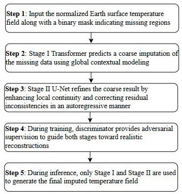
As illustrated in Fig. 1, the architecture of ESTD-Net seamlessly integrates these components to leverage the strengths of both convolutional and transformer-based approaches. The convolutional module efficiently extracts key tokens, while the transformer module utilizes the multi-head context attention mechanism, as outlined in the MAT framework (Li et al., 2022), to capture long-range dependencies between features. This enables more accurate and context-aware reconstructions. The output tokens are further refined through a convolution-based reconstruction module, which restores the spatial resolution to match the input dimensions. The subsequent Conv-U-Net stage enhances local texture continuity and smoothing boundaries by leveraging the local texture refinement capabilities of CNNs, thereby improving the fidelity of the reconstruction. In addition, we have included a concise step-by-step process description, as shown in Fig. 2, which details our workflow, including the input, the two-stage reconstruction process, and the differences between training and inference.

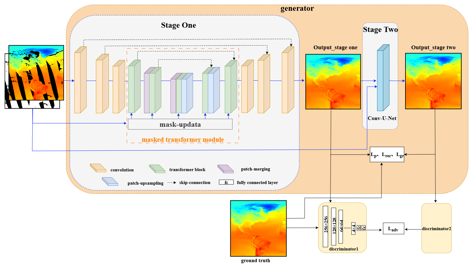
Figure 1 The proposed ESTD-Net framework. In the Stage One, the convolutional module and masked transformer module are employed for feature extraction and initial reconstruction. Patch merging and patch upsampling handle downsampling and upsampling operations, respectively. Stage Two utilizes a convolutional U-Net in an autoregressive manner to refine the coarse output from the Stage One, enhancing local spatial continuity and smoothing boundaries.

Figure 2 The overall workflow of training and inference.

3.2 Convolutional Module

Given a masked temperature field $X_M=X\odot M$, where M is a binary mask assigning a value of 1 to valid (observed) grid points and 0 to missing ones, the goal of the imputation process is to reconstruct spatially coherent and physically plausible values for the missing regions. The convolutional module processes this incomplete field X_M together with the mask M, producing feature maps at a reduced spatial resolution of $\mathrm{1}/\mathrm{4}$ of the original dimensions. These feature maps are then flattened and treated as tokens for subsequent Transformer-based processing.

The module consists of three convolutional layers: one for adjusting the channel dimensions of the input data and two for progressively reducing the spatial resolution. It serves two main purposes: first, to effectively capture the fundamental features of the masked temperature fields; second, by reducing spatial dimensions, it allows the model to focus on large-scale spatial structures while maintaining computational efficiency. On one hand, local spatial context is incorporated a priori in the initial stage of feature extraction to enhance representation quality and overall performance. On the other hand, the reduced resolution significantly lowers computational cost and memory usage. We incorporate a stack of convolutional layers within the convolutional module to extract tokens specifically tailored for the temperature-field imputation task. This design offers several advantages over traditional linear projection methods, such as those used in Vision Transformers (ViT) (Dosovitskiy, 2020), by effectively capturing local spatial patterns and relationships crucial for accurate data reconstruction. The stacked convolutions facilitate a gradual and more effective filling of missing regions in the temperature field, leading to the generation of more informative tokens. Furthermore, multi-scale downsampled features are efficiently passed to the decoder via shortcut connections, which enhances optimization and improves the overall imputation process. In contrast, models that rely solely on linear projections often introduce artifacts and struggle to fully exploit surrounding spatial information for reconstructing missing data.

3.3 Masked Transformer Module

The masked transformer module processes tokens by capturing long-range dependencies between different regions of the temperature field. It consists of five stages, each employing modified transformer blocks to effectively model these spatial relationships. These blocks integrate an enhanced attention mechanism that incorporates additional dynamic masks to guide the process. This attention mechanism enables the model to focus on the most relevant valid regions, thereby improving its ability to restore missing or incomplete temperature data accurately. This design is particularly well-suited for temperature-field imputation tasks, where capturing spatial dependencies across large geographic areas is essential. The dynamic mask further enhances the model's performance by directing its attention towards observed regions, ensuring that the reconstructed values remain physically consistent with the surrounding data. Combined with the multi-stage architecture, this approach significantly improves both the accuracy and spatial coherence of the restored temperature fields.

3.3.1 Context Attention Module based on Mask

To efficiently manage large numbers of tokens and address the low fidelity of individual tokens, the context attention module employs dynamic masks and shifted windows. This design facilitates non-local interactions among a relevant subset of tokens only. The output from the context attention mechanism is computed as a weighted sum of the valid tokens, as follows:

$$\begin{array}{}\text{(1)}& \mathrm{Att}(\mathbf{Q},\mathbf{K},\mathbf{V})=\mathrm{Softmax}\left({\displaystyle \frac{{\mathbf{QK}}^T+{\mathbf{M}}^{\prime }}{\sqrt{d_k}}}\right)\mathbf{V},\end{array}$$

where Q, K, and V are the query, key, and value matrices, respectively, and $\frac{\mathrm{1}}{\sqrt{d_k}}$ is a scale factor. The mask M^′ is defined as:

$$\begin{array}{}\text{(2)}& M_{ij}^{\prime }=\left\{\begin{array}{ll}\mathrm{0},& \text{if token }j\text{ is valid}\\ -\mathit{\tau },& \text{if token }j\text{ is invalid}\end{array}\right.,\end{array}$$

with τ set to a large integer (100 in this experiment) to suppress the impact of invalid tokens. After each attention computation, the w×w windows are shifted by $\left(\frac{w}{\mathrm{2}},\frac{w}{\mathrm{2}}\right)$ pixels, enabling interactions between tokens across different windows. This mechanism facilitates better information flow and enhances the model's ability to capture long-range dependencies.

Mask Update

The mask M^′ evolves dynamically across layers to represent the validity of tokens, enabling the model to selectively focus on relevant regions of the temperature field. Initially, M^′ is identical to the input observation mask; however, it progressively adapts during each propagation step, ensuring that the model's attention remains directed toward physically valid and meaningful areas throughout the process. The key aspect of our approach is the adaptive propagation rule: if a spatial window contains at least one valid token, all tokens within that window are considered valid after the attention operation. Conversely, windows without any valid tokens remain invalid, ensuring that attention is concentrated only on sparse but relevant regions where additional information is most needed.

As illustrated in Fig. 3, this process starts with localized validity (from (a) to (b)) and gradually expands the valid regions through successive window shifts and attention passes. This adaptive mask update scheme allows the mask to progressively cover the entire spatial domain, optimizing token propagation and enhancing the model's capability to capture long-range spatial dependencies for more accurate temperature-field reconstruction.

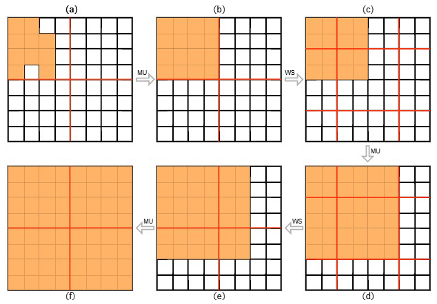
Figure 3 The mask updating process. Orange represents valid areas and white represents invalid areas. Initially, the spatial domain is divided into 4×4 regions (highlighted in red). MU represents the mask update that occurs following the attention mechanism and WS denotes the window shift operation.

Operational Process

The operational logic of the mask-based contextual attention mechanism is further illustrated in Fig. 4. The pseudocode representation outlines how missing values are reconstructed by attending to valid regions within a local spatial window. Specifically, for each masked region, the attention weights are computed only over valid tokens, and the missing tokens are iteratively updated based on the similarity and spatial correlation with observed neighbors. This formulation allows the model to effectively propagate contextual information and maintain spatial coherence during reconstruction.

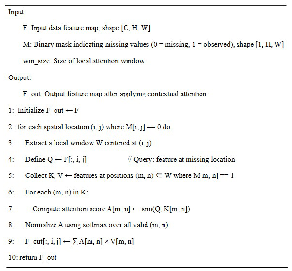
Figure 4 Illustration of the mask-based contextual attention mechanism. The pseudocode outlines how missing tokens are reconstructed by attending to valid spatial regions within the local window.

3.3.2 Modified Transformer Block

In conventional transformer architectures (Vaswani et al., 2017), each block consists of two essential components: multi-head self-attention and multi-layer perceptron. Typically, layer normalization (LN) is applied prior to each block, and a residual connection (He et al., 2016) is incorporated after each operation. However, when dealing with masks that contain large missing regions, we have observed that the standard block structure often results in unstable optimization, including instances of gradient explosion. This instability can be primarily attributed to the high proportion of invalid tokens, which are close to zero. In such scenarios, layer normalization tends to disproportionately amplify these near-zero tokens, leading to training instability. Furthermore, the residual connections in conventional transformers generally encourage the model to focus on high-frequency content, which may not be optimal for inpainting tasks that require smooth and coherent reconstructions. Given that a significant number of tokens are initially invalid, directly learning high-frequency features becomes challenging. A stable optimization process typically requires a robust low-frequency foundation, especially in GAN training, to ensure reliable convergence and avoid instability.

To address these challenges, we propose a modified transformer block specifically designed to optimize masks with missing regions. In this approach, we replace residual connections with concatenation and eliminate layer normalization altogether. As illustrated in Fig. 5, our method concatenates the output processed by context attention with the unprocessed input before passing it through a fully connected layer:

$$\begin{array}{}\text{(3)}& {\mathbf{X}}_{r,\mathrm{\ell }}=\mathrm{MLP}\left[\mathrm{FC}\left(\left[\mathrm{MCA}\left({\mathbf{X}}_{r,\mathrm{\ell }-\mathrm{1}}\right),{\mathbf{X}}_{r,\mathrm{\ell }-\mathrm{1}}\right]\right)\right],\end{array}$$

where X_r,ℓ is the output of multi-layer perceptron at the ℓth block in the rth stage. After passing through several modified transformer blocks, as shown in Fig. 5, we introduce a convolutional layer with a global residual connection. Additionally, we cancel positional embeddings in our transformer design. Previous studies (Wu et al., 2021; Xie et al., 2021) have demonstrated that 3×3 convolutions can incorporate positional information into transformers. Consequently, feature interactions are primarily driven by feature similarity, which strengthens long-range dependencies and facilitates more effective interactions within the data.

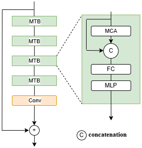
Figure 5 Illustration of a single transformer stage, where MTB denotes the modified transformer block, and MCA refers to the context attention module.

3.4 Loss Functions

To enhance the quality of the generated content, we employ adversarial loss (Mirza and Osindero, 2014) in both stages of our framework. This loss function guides the model in generating more realistic outputs by encouraging the generator to produce content that closely resembles real data, as evaluated by the discriminator. Additionally, we incorporate perceptual loss (Johnson et al., 2016) with a reduced empirical coefficient, as we have observed that this modification improves both optimization stability and effectiveness. Furthermore, perceptual loss directs the model to focus on high-level feature similarities between the generated and ground-truth data, thereby enhancing perceptual quality, particularly in the reconstruction regions. To optimize the quality of generated data, we calculate the adversarial loss as follows:

$$\begin{array}{}\text{(4)}& {\displaystyle }{\mathcal{L}}_G=-{\mathbb{E}}_{\widehat{x}}\left[\log \right(D\left(\widehat{x}\right)\left)\right],\text{(5)}& {\displaystyle }{\mathcal{L}}_D=-{\mathbb{E}}_x\left[\log \right(D\left(x\right)\left)\right]-{\mathbb{E}}_{\widehat{x}}\left[\log \right(\mathrm{1}-D\left(\widehat{x}\right)\left)\right],\text{(6)}& {\displaystyle }{\mathcal{L}}_{\mathrm{adv}}={\mathcal{L}}_D+{\mathcal{L}}_G+\mathit{\alpha }{\mathcal{L}}_{gp},\end{array}$$

where x represents the real data and $\widehat{x}$ (the generated data) is defined as $\widehat{x}=G\left(x\right)$. The gradient penalty L_gp is given by $L_{\text{gp}}={\mathbb{E}}_{\widehat{x}}{∥{\mathrm{\nabla }}_{\widehat{x}}D\left(\widehat{x}\right)∥}^{\mathrm{2}}$ (Gulrajani et al., 2017) , enhances the stability of the model during training and helps mitigate the risk of overfitting with α=0.001.

To reduce the difference between real data and generated data, we utilize the high-level features of the pretrained VGG-19 (Simonyan, 2014) to construct the perceptual loss:

$$\begin{array}{}\text{(7)}& {\mathcal{L}}_P=\sum _{i=\mathrm{4}}^{\mathrm{5}}{\mathit{\eta }}_i{∥{\mathit{\varphi }}_i\left(\widehat{x}\right)-{\mathit{\varphi }}_i\left(x\right)∥}_{\mathrm{1}},\end{array}$$

where ϕ_i(⋅) represents the activation of layer i in a pre-trained VGG-19 network η_i are non-negative parameters.

For the task of reconstructing global surface temperature data – which exhibits comprehensive spatial coverage but suffers from temporal sparsity and extensive missing values, we propose an improved loss function architecture based on generative adversarial networks (GANs). The primary challenge associated with this dataset stems from the coexistence of spatial continuity and temporal fragmentation, necessitating not only accurate imputation of missing temperature values but also seamless spatial and temporal transitions between observed and reconstructed regions. To address these challenges, we introduce two key modifications to the loss function, which collectively enhance the precision of temperature reconstruction while ensuring physically consistent and smooth gradients across discontinuities. In order to improve the accuracy of temperature reconstruction in missing regions, we define a weighted reconstruction loss function:

$$\begin{array}{}\text{(8)}& {\mathcal{L}}_{\mathrm{rec}}={\displaystyle \frac{{∥\mathbf{M}\otimes \left(\mathit{x}-\widehat{\mathit{x}}\right)∥}_{\mathrm{1}}}{\mathit{\varsigma }{∥\mathbf{M}∥}_{\mathrm{1}}}}+{\displaystyle \frac{{∥\left(\mathbf{1}-\mathbf{M}\right)\otimes \left(\mathit{x}-\widehat{\mathit{x}}\right)∥}_{\mathrm{1}}}{{∥\mathbf{1}-\mathbf{M}∥}_{\mathrm{1}}}},\end{array}$$

where x represents ground-truth, $\widehat{\mathit{x}}$ represents generated data, and M represents mask. ς is the weight between the known and missing data. This approach ensures that the reconstruction of missing regions closely aligns with the original data, while preserving consistency in the known areas. Similar to mask-based reconstruction losses used in image restoration tasks, this weighted loss method is particularly well-suited for surface temperature data reconstruction, effectively avoiding unnatural temperature gradients.

To improve the physical plausibility and visual coherence of inpainted data, we introduce a novel gradient regularization loss L_gr, designed to minimize the L1 norm of the gradient difference between the generated output $\widehat{\mathit{x}}$ and the ground truth x. The loss is formally defined as:

$$\begin{array}{}\text{(9)}& L_{\text{gr}}=\Vert \mathrm{\nabla }\left(x\right)-\mathrm{\nabla }\left(\widehat{x}\right){\Vert }_{\mathrm{1}}.\end{array}$$

By integrating gradient consistency regularization, our model learns to produce reconstructions that maintain both visual smoothness and physical fidelity with respect to the observed data. This constraint is particularly crucial in applications where gradient structures, such as temperature fronts or atmospheric transitions, play a key role in data interpretation.

The overall first stage loss functions is:

$$\begin{array}{}\text{(10)}& L=L_{\mathrm{adv}}+\mathit{\eta }{L}_P+\mathit{\lambda }{L}_{\text{rec}}+\mathit{\beta }{L}_{\text{gr}},\end{array}$$

where η, λ and β are non-negative parameters. The total losses in the second stage are consistent with those in the first stage.Given that our framework employs two discriminators across dual stages, potential instability during adversarial training was carefully addressed. To enhance convergence stability, we applied R1 gradient penalty to both discriminators, maintained an exponential moving average (EMA) of generator weights to smooth updates, and adopted adaptive data augmentation (ADA) to prevent discriminator overfitting (Li et al., 2022). These strategies collectively ensured stable training without divergence or mode collapse.

4 Experiments

4.1 Datasets and Metrics

The reference dataset employed in this study originates from the Microwave Radiation Imager (MWRI) aboard the FengYun-3D (FY-3D) satellite. As a passive microwave sensor, MWRI offers distinct advantages for near-surface temperature retrieval: (1) its low-frequency channels can penetrate most non-precipitating clouds, and (2) the peak sensitivity of its weighting functions occurs close to the surface level. These characteristics make MWRI particularly suitable for monitoring lower atmospheric and surface temperature.

The analysis focuses on the full calendar year of 2023. FY-3D operates in an afternoon orbit with an equatorial crossing time of approximately 14:00 UTC. To improve temporal representativeness, MWRI retrievals are processed into two global datasets centered at 06:00 and 18:00 UTC, by aggregating the nearest available observations within ±3 h of each reference time. This yields a twice-daily global gridded surface temperature product at 0.5° × 0.5° spatial resolution. Because MWRI's narrow swath leaves large orbital gaps and frequent data voids under cloudy conditions, direct evaluation against in situ measurements is infeasible. Therefore, we employ ERA5 reanalysis surface temperature as the reference baseline for quantitative assessment. ERA5 is selected for three main reasons: (1) its high temporal resolution (hourly), enabling precise temporal alignment with MWRI overpasses; (2) its proven reliability and widespread adoption in climate research; and (3) its global coverage, which allows retrieval of complete “truth” values in regions where MWRI lacks observations.

To construct a benchmark dataset that realistically mimics MWRI's missing-data patterns while retaining access to ground-truth values, we proceed as follows: (1) ERA5 hourly surface temperature data are interpolated to match the 0.5° × 0.5° MWRI retrieval grid, ensuring precise spatial alignment. (2) For each MWRI time slice, we generate a validity mask based on actual MWRI coverage, retaining ERA5 values only at grid points where valid MWRI retrievals exist, and masking the rest to simulate orbital gaps and missing observations. (3) The masked ERA5 fields serve as the synthetic “MWRI-like” inputs with gaps, while the corresponding full, unmasked ERA5 fields provide the ground-truth reference for evaluating reconstruction accuracy in the missing regions.

The primary focus of this investigation centers on developing effective reconstruction methods for satellite orbital gaps (vacancies). Through careful spatiotemporal matching, we ensure accurate localization of these data voids for subsequent analysis and repair.

To facilitate model training and enhance intercomparability of temperature values, we applied global min-max normalization to standardize the data range. The normalization process follows:

$$\begin{array}{}\text{(11)}& X_{\text{norm}}={\displaystyle \frac{X-X_{min}}{X_{max}-X_{min}}},\end{array}$$

where X denotes the original temperature values, with X_min and X_max representing the global minimum and maximum temperatures across the entire dataset, respectively. This transformation maps all values to the interval [0,1], ensuring numerical stability during model optimization while preserving the relative thermal gradients.

The normalized dataset was systematically partitioned into 256×256 regions, a size selected to balance computational efficiency with sufficient spatial context for pattern recognition. From each original data file, we extracted six non-overlapping subregions through a sliding window approach, yielding a total of 4374 analyzable units. The complete dataset was randomly partitioned into training and test sets containing 3600 and 774 samples respectively, maintaining an approximately 4:1 ratio to ensure sufficient representation in both subsets. To comprehensively assess the reconstruction performance, we implemented four established evaluation metrics: mean absolute error (MAE), root mean square error (RMSE), peak signal-to-noise ratio (PSNR), and structural similarity index (SSIM). Each of these metrics offers a unique perspective on the accuracy and quality of the reconstructed data.

• Mean Absolute Error (MAE). MAE is a metric that quantifies the average magnitude of errors between the reconstructed data and the ground truth, without accounting for their direction. It offers a clear understanding of the average deviation of predicted values from actual values, making it particularly useful for evaluating overall reconstruction accuracy. The formula for MAE is:

  $$\begin{array}{}\text{(12)}& \text{MAE}={\displaystyle \frac{\mathrm{1}}{n}}\sum _{i=\mathrm{1}}^n|x_i-\widehat{x_i}|,\end{array}$$

  where x_i represents the ground truth values, $\widehat{x_i}$ the predicted values, and n the number of samples.

• Root Mean Square Error (RMSE). RMSE is similar to MAE, but it places greater emphasis on larger errors by squaring the differences before averaging. This makes RMSE more sensitive to outliers and particularly valuable when minimizing large reconstruction errors is a priority. The formula for RMSE is:

  $$\begin{array}{}\text{(13)}& \text{RMSE}=\sqrt{{\displaystyle \frac{\mathrm{1}}{n}}\sum _{i=\mathrm{1}}^n(x_i-\widehat{x_i}{)}^{\mathrm{2}}}.\end{array}$$

  Both MAE and RMSE assess the overall reconstruction error, with RMSE placing greater emphasis on larger deviations due to its sensitivity to outliers. Together, these metrics offer complementary perspectives on the quality of the reconstruction.

• Peak Signal-to-Noise Ratio (PSNR). PSNR is a widely used metric for evaluating the quality of image reconstruction. It compares the maximum possible pixel value of an image (MAX) to the mean squared error (MSE) between the ground truth and generated images. Higher PSNR values indicate better reconstruction quality, with less distortion. The formula for PSNR is:

  $$\begin{array}{}\text{(14)}& \text{PSNR}=\mathrm{20}\cdot {\log }_{\mathrm{10}}\left({\displaystyle \frac{\text{MAX}}{\text{RMSE}}}\right).\end{array}$$

• Structural Similarity Index (SSIM). SSIM evaluates the perceptual quality of the reconstructed data by considering changes in structural information, luminance, and contrast. Unlike MSE and RMSE, which focus on absolute pixel differences, SSIM assesses the similarity between corresponding pixels based on their structural, brightness, and contrast characteristics. This makes SSIM a more accurate measure of image quality in terms of human visual perception. The formula for SSIM is:

  $$\begin{array}{}\text{(15)}& \text{SSIM}(x,\widehat{x})={\displaystyle \frac{(\mathrm{2}{\mathit{\mu }}_x{\mathit{\mu }}_{\widehat{x}}+c_{\mathrm{1}})(\mathrm{2}{\mathit{\sigma }}_{x\widehat{x}}+c_{\mathrm{2}})}{({\mathit{\mu }}_x^{\mathrm{2}}+{\mathit{\mu }}_{\widehat{x}}^{\mathrm{2}}+c_{\mathrm{1}})({\mathit{\sigma }}_x^{\mathrm{2}}+{\mathit{\sigma }}_{\widehat{x}}^{\mathrm{2}}+c_{\mathrm{2}})}},\end{array}$$

  where μ_x and ${\mathit{\mu }}_{\widehat{x}}$ are the mean pixel values of the original and generated images, σ_x and ${\mathit{\sigma }}_{\widehat{x}}$ are their variances, ${\mathit{\sigma }}_{x\widehat{x}}$ is the covariance between the two images, and c₁ and c₂ are constants to stabilize the division when the denominator is close to zero.

These four metrics provide a comprehensive evaluation of the model's performance, capturing both pixel-level accuracy and perceptual quality. By integrating these metrics, we ensure a thorough assessment of the reconstructed images, considering both numerical precision and perceptual realism.

4.2 Implementation Details

All experiments were conducted using two NVIDIA A6000 GPUs. The model was trained on the processed ERA5 reanalysis dataset, with a batch size of 32 to optimize training efficiency. During training, we set the learning rate to 0.001. We employed the Adam optimizer, a widely used choice in deep learning, due to its effectiveness in managing sparse gradients and adapting learning rates for individual parameters. ς, η, λ and β are set as 10, 0.1,10 and 0.01, respectively.

4.3 Comparative assessment

In this section, we evaluate the effectiveness of our proposed reconstruction method, ESTD-Net, through a comparative analysis with both traditional and deep learning-based approaches. For traditional reconstruction methods, we selected a technique based on spatial information to minimize manual intervention. Specifically, we employed inverse distance-weighted interpolation(IDW) (Kilibarda et al., 2014), a simple yet effective spatial data interpolation method.

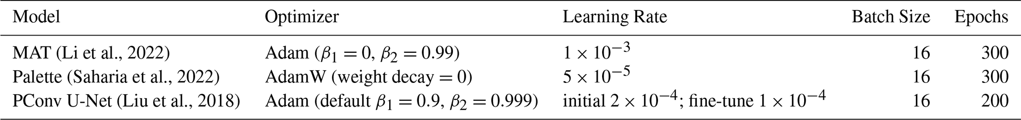
For deep learning-based reconstruction, we utilized Partial Convolutions combined with the U-Net architecture (Liu et al., 2018), which is well-suited for handling irregularly shaped missing regions in data recovery. Previous studies have demonstrated that U-Net with partial convolutions outperforms alternative methods such as PatchMatch (Barnes et al., 2009), convolutional U-Net architectures with varying null-value initializations, and extended frameworks like Content Encoders (Iizuka et al., 2017), which incorporate both global and local discriminators along with Poisson blending as a post-processing step. Additionally, Yu et al. (2018) proposed replacing post-processing with a refinement network that utilizes context attention layers. Despite these alternatives, U-Net with partial convolutions remains the preferred choice due to its superior ability to handle irregular gaps, making it particularly effective for reconstruction tasks. In addition, we also included Palette (Saharia et al., 2022) (an advanced diffusion-based restoration model) and MAT (Li et al., 2022) (a model that focuses on reconstruction of masked areas) in the experimental comparison. The detailed training configurations of these deep learning-based models are summarized in Table 1.

(Li et al., 2022)(Saharia et al., 2022)(Liu et al., 2018)

Table 1 Training configurations of baseline models used for comparative experiments. All models were retrained from scratch on our dataset under identical data splits and masking configurations as ESTD-Net.

The quantitative evaluation results are summarized in Table 2. From the results, we can find that our method can obtain more accurate results. To further assess the performance of our method, we conducted a qualitative analysis by visually comparing the reconstruction results of ESTD-Net with those of other reconstruction approaches. As illustrated in Fig. 6, ESTD-Net demonstrates superior reconstruction capabilities, particularly in preserving the structural continuity of missing regions. Specifically, our method effectively smooths the boundaries of missing areas, mitigates artifacts commonly observed in conventional interpolation methods, and accurately reconstructs the internal spatial patterns within these regions. Furthermore, ESTD-Net exhibits a strong capacity to capture zonal gradient variations in Sea Surface Temperature (SST), ensuring consistency with large-scale oceanic temperature structures.

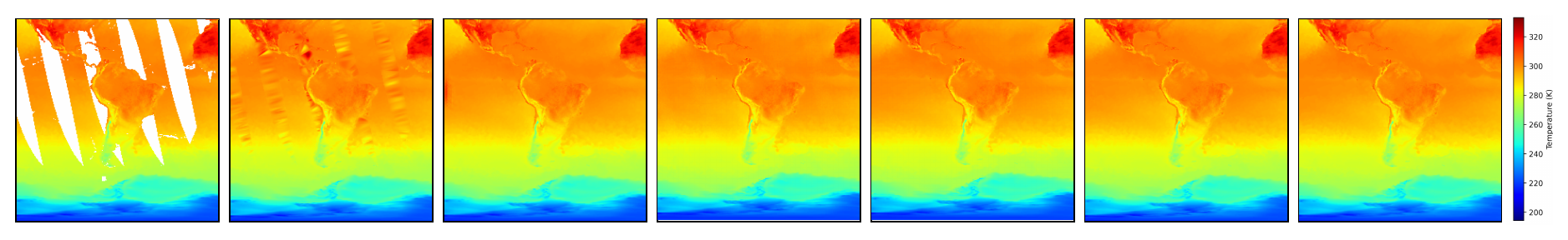
Figure 6 Reconstruction Results of Surface Temperature. From left to right, the columns display the initial incomplete data, the results of inverse distance weighting (IDW) interpolation, the results from partial convolution U-Net (Pconv U-Net), the results from Palette, the results from MAT,the results from our proposed method, and the ground truth. All panels utilize identical color scaling to facilitate direct visual comparison.

To further highlight the advantages of our method, we compute the absolute differences between the reconstructed results and the true values for each approach. To amplify these differences, we apply the logarithm to the absolute error plus one, where the addition of one helps avoid negative infinity values resulting from zero errors. The difference maps, presented in Fig. 7, provide a detailed visualization of the reconstruction errors. Compared to traditional and deep learning-based methods, ESTD-Net significantly reduces errors along the edges of missing regions, better preserves temperature gradients, and maintains physically plausible spatial patterns. These improvements underscore the model's ability to leverage both spatial and temporal correlations for more accurate and reliable SST reconstructions.

Table 2 Comparison of different methods.

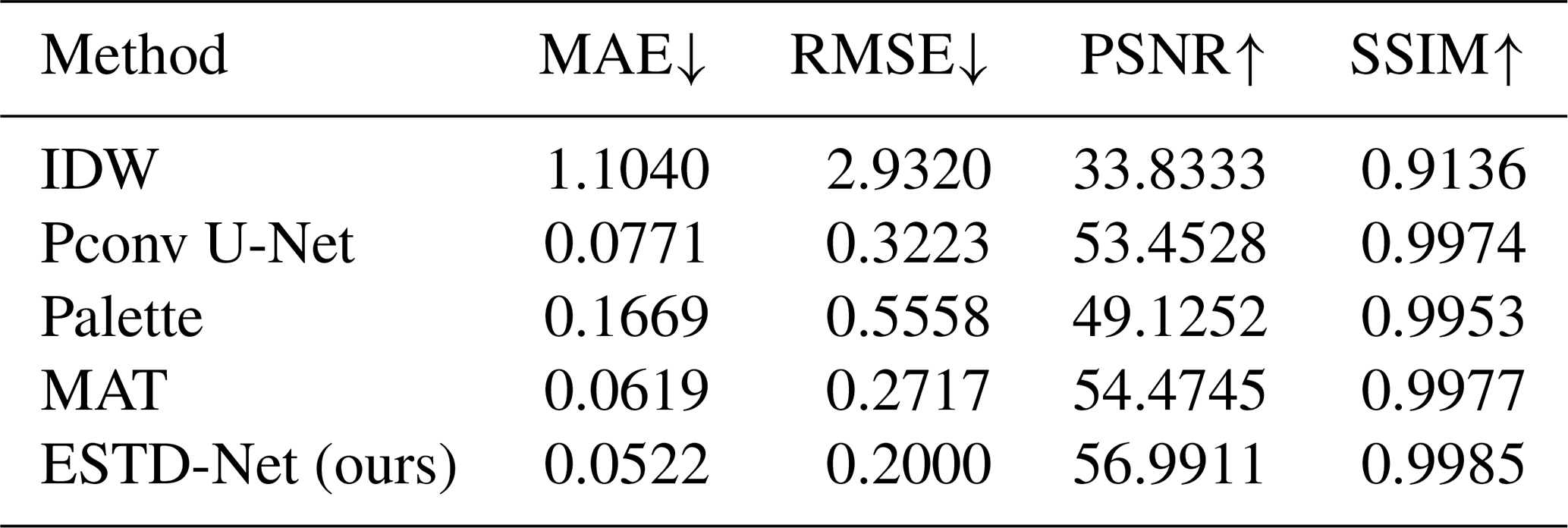
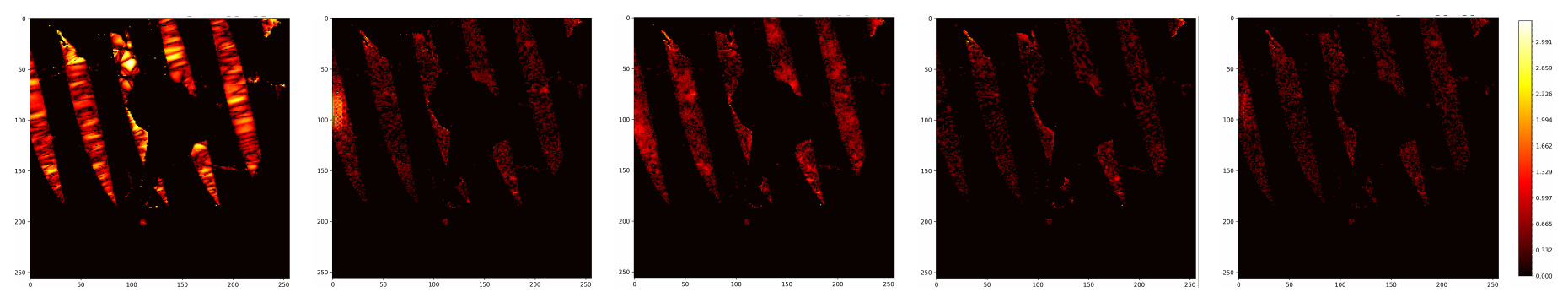
Figure 7 Comparison of Different Methods with Ground Truth. From left to right, the columns display the difference of the reconstructed data of IDW, Pconv_U-net, Palette, MAT and our method with those of the ground truth.

4.4 Ablation and analysis

In this section, we present a detailed analysis of its performance metrics, highlighting the model's superior results and elucidating the contributions of each key component. To systematically evaluate the impact of different loss function components on reconstruction performance, we conducted an ablation study focusing on the Weighted Reconstruction Loss and Gradient Consistency Regularization. In satellite-based temperature retrieval, missing data typically arise from factors such as cloud contamination and orbital gaps. In our approach, we employ various weighting schemes for the reconstruction loss to emphasize the restoration of these missing regions. Specifically, we compare a baseline model that incorporates adversarial loss and perceptual loss against models that introduce a weighting ratio for masked (missing) to unmasked (observed) areas in the reconstruction loss. This weighting ensures a stronger emphasis on missing regions, which is crucial for effectively filling large gaps in Earth Surface Temperature data.

Additionally, we examine the effect of incorporating Gradient Consistency Regularization, which enforces smooth transitions and structural coherence in the reconstructed regions. The results, summarized in Table 3, demonstrate the effectiveness of the proposed loss terms. Compared to the baseline model, which achieves a Mean Absolute Error (MAE) of 0.0669, incorporating the Weighted Reconstruction Loss significantly reduces MAE to 0.0553, representing a 17.3 % reduction. Similarly, the Root Mean Square Error (RMSE) decreases from 0.2658 to 0.2177, and Peak Signal-to-Noise Ratio (PSNR) improves from 55.1125 to 56.4303 dB, indicating enhanced reconstruction accuracy. The inclusion of Gradient Consistency Regularization further refines these results: the full model achieves an MAE of 0.0522 and an RMSE of 0.2000, corresponding to overall reductions of 22.0 % and 24.7 %, respectively, relative to the baseline model. These improvements suggest that our approach not only minimizes pixel-level errors but also enhances the physical consistency of Sea Surface Temperature (SST) patterns by better preserving zonal temperature gradients and reducing discontinuities at the boundaries of missing regions.

Table 3 Ablation study on the effect of loss functions.

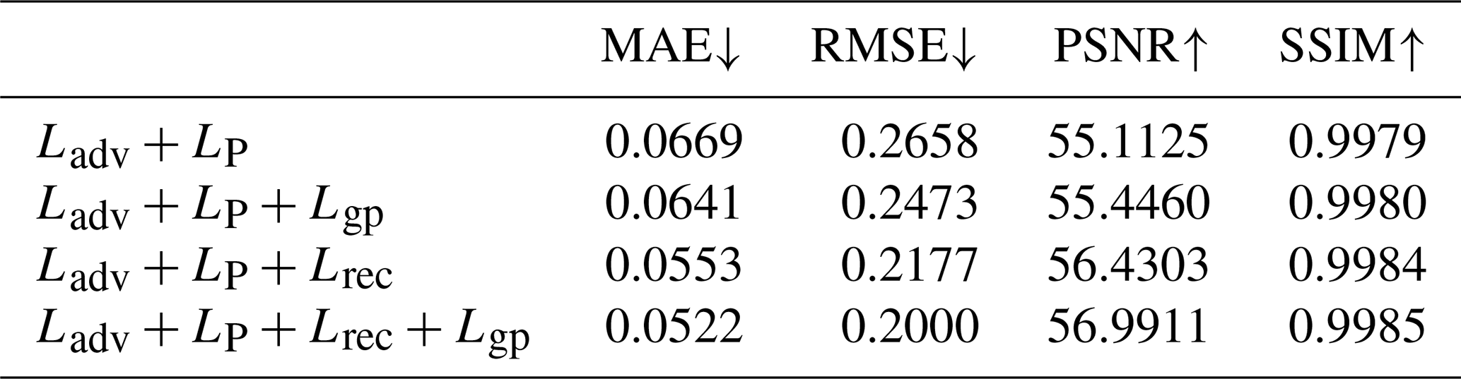
As shown in Table 3, the combination of adversarial loss, perceptual loss, and weighted reconstruction loss achieves the best performance among the various configurations. This combination results in the lowest MAE and RMSE, while also yielding the highest PSNR and SSIM. These results underscore the significance of the weighted reconstruction loss in guiding the model to accurately reconstruct missing regions, thereby significantly enhancing overall performance. The introduction of Gradient Consistency Regularization, which minimizes gradient discrepancies between the ground truth and reconstructed data, further improves perceptual quality, as evidenced by the increased PSNR and SSIM scores. This regularization term helps maintain smooth transitions and structural integrity within the reconstructed data. Notably, its effect is most pronounced when combined with other loss components, highlighting the synergistic benefits of this multi-loss framework.

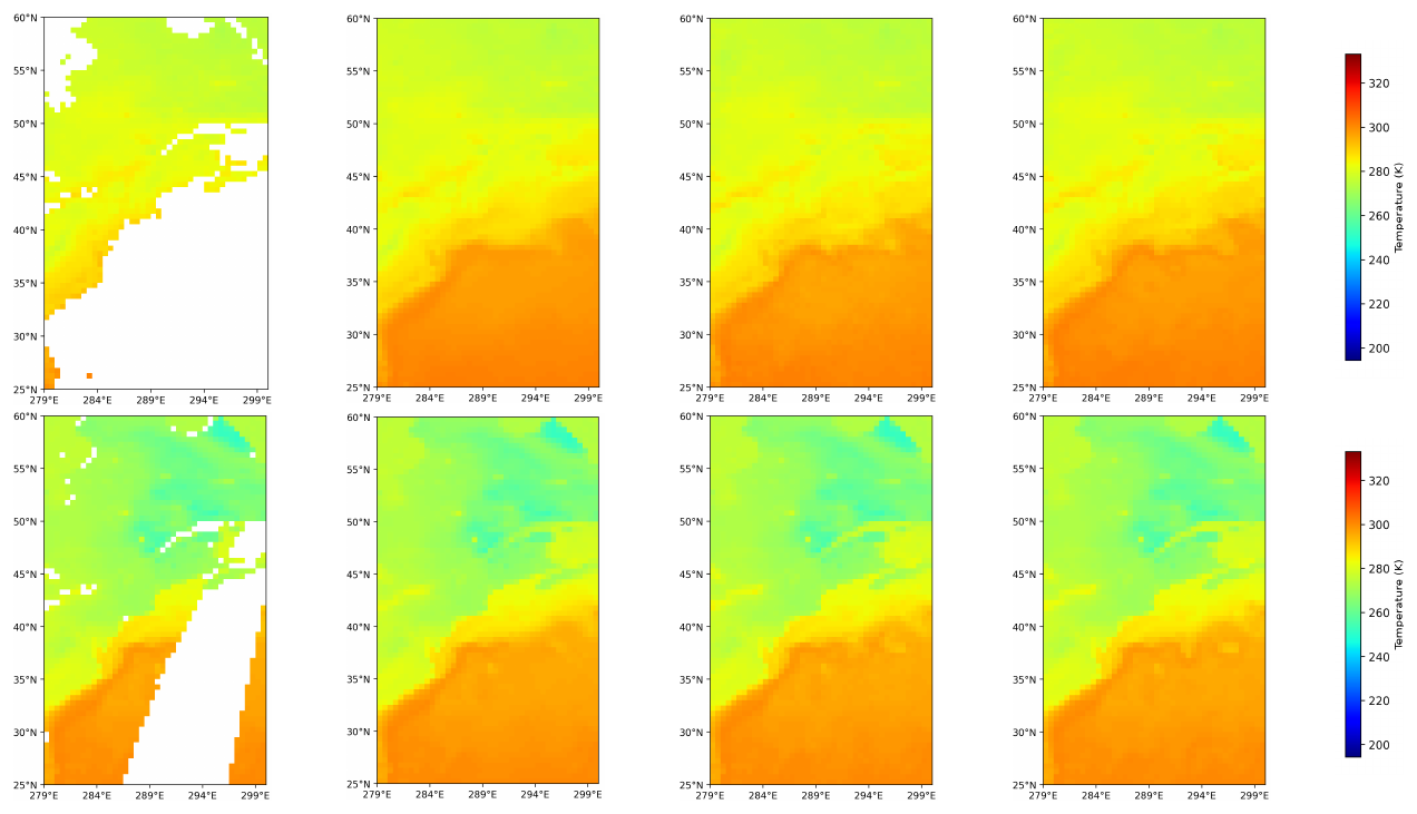
Figure 8 Comparison of Gradient Settings on different missing ratios. From left to right, the columns display the initial data, the reconstruction result without gradient settings, the reconstruction result with gradient settings applied, and the ground truth. The white regions in the original data indicate missing values.

Overall, the integration of adversarial loss, perceptual loss, weighted reconstruction loss, and Gradient Consistency Regularization results in a well-balanced performance that enhances both pixel-level accuracy and perceptual quality in the reconstructed EST data. These findings demonstrate the robustness of our model in handling large-scale missing data while effectively capturing complex spatial and temporal dependencies within the EST data.

The experimental results underscore the critical roles of both weighted reconstruction loss and gradient consistency regularization in enhancing performance in the surface temperature image inpainting task. The weighted reconstruction loss, by prioritizing errors in the unmasked regions, is essential for improving the overall quality of the reconstruction. Meanwhile, gradient consistency regularization enhances the structural coherence of the generated images, thereby improving both the overall quality and structural consistency of the inpainting results.

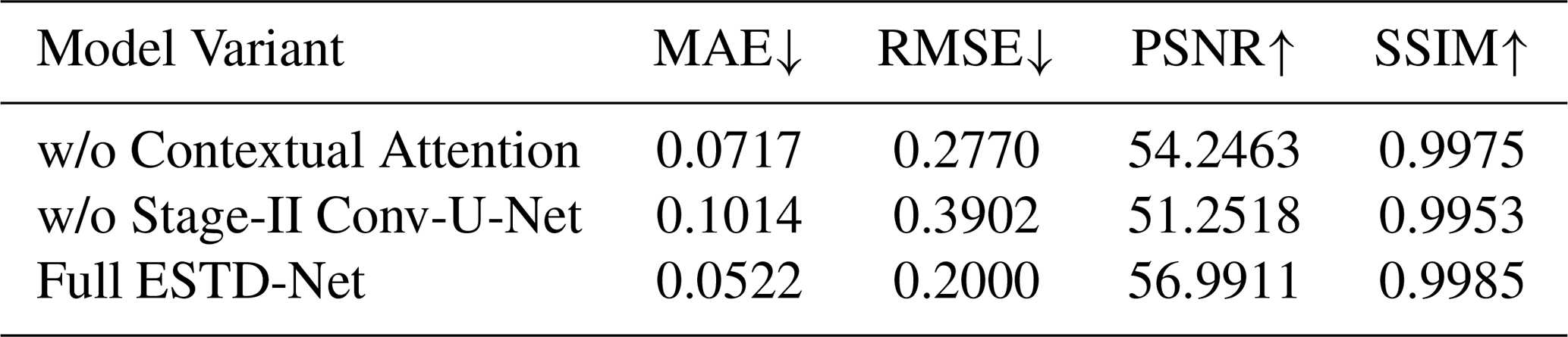
To verify the effects of the dedicated mask-based context attention module and the Stage II Conv-U-Net, we conducted relevant ablation experiments. The specific results are shown in Table 4. Removing the context attention would increase the mean absolute error from 0.0522 to 0.0717, and reduce the peak signal-to-noise ratio from 56.9911 decibels to 54.2463 decibels. Omitting the second-stage convolutional U-network would further degrade the performance (mean absolute error 0.1014, peak signal-to-noise ratio 51.2518 decibels). These verification experiments confirmed the crucial contributions of these two modules to the reconstruction quality of the ESTD network.

Table 4 Comparison of model variant.

4.4.1 Gradient setting comparison

To evaluate the effectiveness of gradient consistency regularization in preserving physically meaningful structures, we conducted a focused assessment over the eastern coastline of North America and the adjacent Atlantic Ocean, a region characterized by sharp land-sea thermal contrasts. This area spans latitudes from 25 to 60° N and longitudes from 279 to 300° E, exhibiting pronounced temperature gradients at coastal boundaries, thereby making it an ideal testbed for evaluating boundary reconstruction performance.

As illustrated in Fig. 8, the inclusion of the gradient consistency regularization term significantly enhances the model's ability to capture fine-scale temperature variations. The white regions in the original data indicate missing values. Specifically, this term promotes the alignment of gradient structures between the generated output and the ground truth, resulting in sharper transitions and improved preservation of boundary features. In comparison to the reconstruction result without this setting (Column 2), the model incorporating gradient consistency regularization (Column 3) demonstrates clearer and more continuous land-sea edges, more accurately reflecting the ground truth (Column 4). This enhancement is particularly evident in the recovery of temperature fronts and the retention of cross-boundary gradients, which are often smoothed out or distorted in models lacking explicit gradient guidance. Such improvements illustrate that this regularization not only enhances the visual coherence of the restored data but also contributes to the physical plausibility of the reconstructed temperature field, an essential aspect for downstream geoscientific analyses where maintaining spatial gradient integrity is critical.

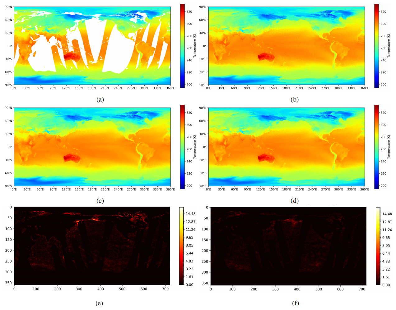
Figure 9 Reconstructed data of Stage Two steps. (a) Initial data. (b) Ground truth. (c) Result of the first stage. (d) Result of the second stage. (e) Difference Between the reconstructed data of the first stage and the ground truth. (f) Difference Between the reconstructed data of the second stage and the ground truth.

4.4.2 Hyperparameter analysis

Regarding the selection of the hyperparameters α in the gradient penalty term and β in the gradient consistency regularization term, we conducted sensitivity experiments by choosing different values for these hyperparameters. The results are shown in Tables 5 and 6. The analysis results indicate that the performance is relatively stable within a wide range of values, but our chosen hyperparameters yield the best results.

Table 5 Sensitivity analysis of the gradient penalty coefficient α.

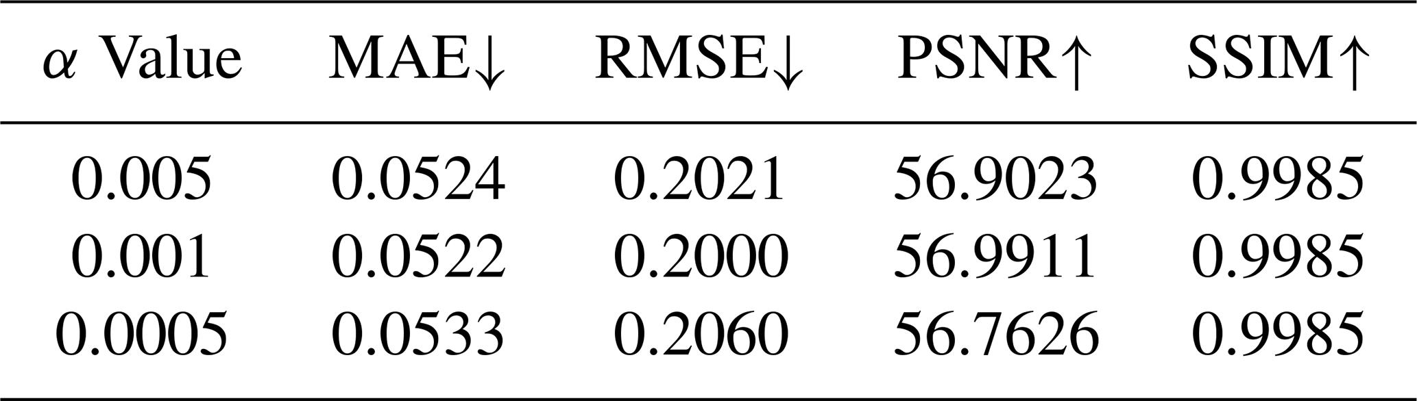
Table 6 Sensitivity analysis of the gradient consistency coefficient β.

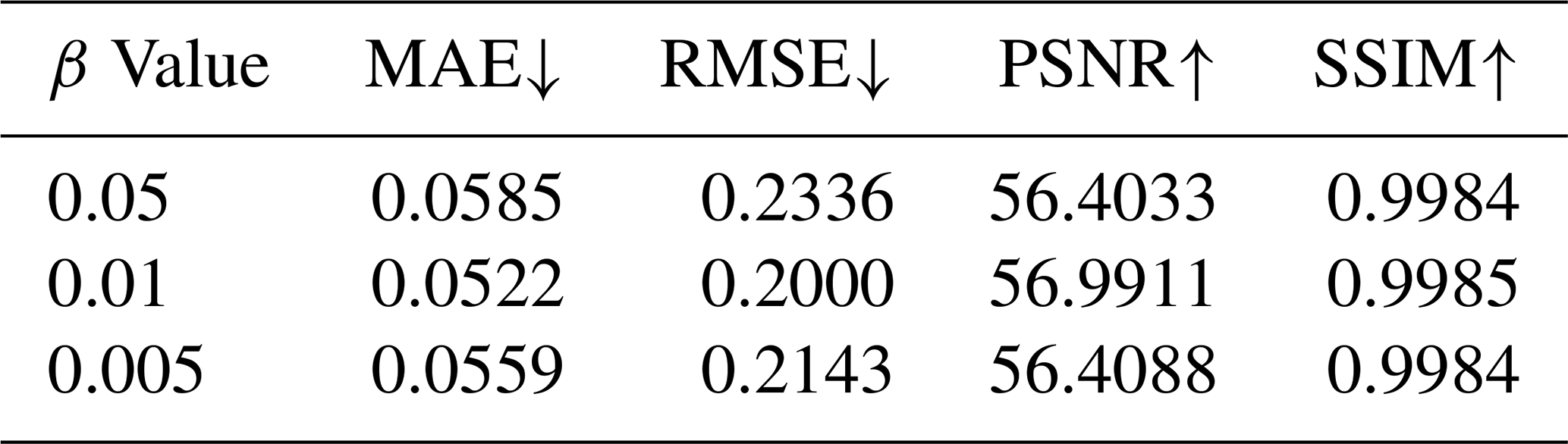
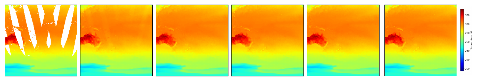
Figure 10 Reconstruction Results of Surface Temperature. From left to right, the columns display the initial incomplete data, the results from Palette, the results from PConv U-Net, the results of MAT, the results from our proposed method, and the ground truth.

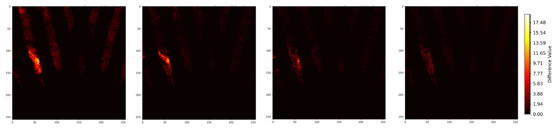
Figure 11 Comparison of Different Methods with Ground Truth. From left to right, the columns display the difference of the reconstructed data of Palette, PConv U-Net, MAT and our method with those of the ground truth.

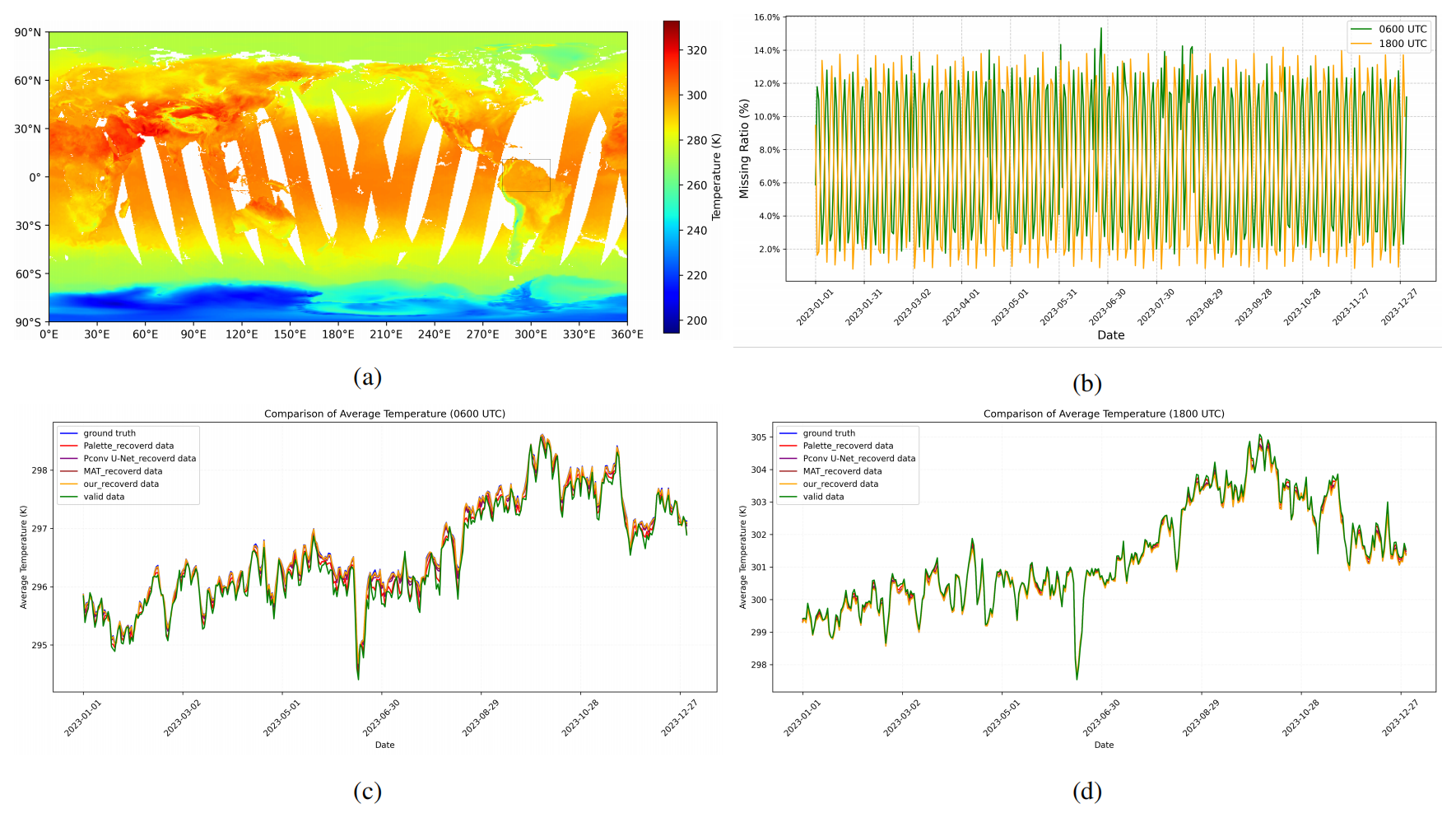
Figure 12 Temporal stability and multi-model comparison of average surface temperature reconstruction in the selected eastern Pacific region. (a) Global spatial distribution of Earth Surface Temperature, with the chosen region (282–312° E, 10° N–10° S) outlined in black. (b) Missing data rates over the entire year of 2023 at 06:00 and 18:00 UTC in the selected region. (c–d) Comparison of regional average temperatures across different models – Palette (Saharia et al., 2022), PConv U-Net (Liu et al., 2018), MAT (Li et al., 2022), our proposed ESTD-Net, valid (non-missing) data, and ground truth – at 06:00 and 18:00 UTC, respectively. The blue, red, purple, brown, orange, and green lines correspond to the average temperatures of the ground truth, Palette, PConv U-Net, MAT, our proposed method, and the valid (non-missing) data before reconstruction, respectively.

4.4.3 The role of the Second Stage

The interpolated data generated in the first stage is produced by applying adaptive weights to valid pixels within local windows. While this method can restore the overall temperature field, it often results in imprecise outputs in regions with complex spatial variations, leading to localized artifacts and inconsistent transitions. To address these issues, we introduce a convolutional U-Net in the second stage to autoregressively refine the initial results. This refinement process aims to enhance local continuity and correct structural inconsistencies.

As illustrated in Fig. 9, a direct visual comparison of the global outputs from the first and second stages (Fig. 9c and d) reveals only subtle differences. However, the absolute difference maps relative to the ground truth (Fig. 9e and f) more clearly highlight the improvements achieved by the second stage. In Fig. 9e, the absolute error between the first-stage output and the ground truth displays numerous scattered high-magnitude differences, reflecting the limitations of local window-based interpolation in accurately capturing detailed spatial structures.

In contrast, the absolute difference shown in Fig. 9f is notably smoother and less concentrated, indicating that the second-stage U-Net effectively reduces local anomalies and refines spatial transitions. This improvement is particularly evident in areas characterized by sharp temperature gradients or complex patterns, where the second-stage refinement yields results that align more closely with the physical characteristics of the temperature field. These enhancements demonstrate that the convolutional U-Net plays a crucial role in improving reconstruction quality by minimizing abrupt local deviations and producing smoother, more physically plausible outputs.

4.4.4 Comparison of Edge-Case Temperature Variations

To verify the data recovery performance of our model in regions with extreme temperature variations, we conducted a set of experiments. These regions were selected manually and randomly masked in the temperature map. These regions were chosen based on obvious high spatial gradients (for example, the boundary areas between land and sea). We compared the performance of ESTD-Net with three powerful baseline models (Palette, PConv U-Net, and MAT), and the results are shown in Fig. 10. Additionally, we also compared the absolute error graphs of the reconstructed outputs with the true values, and the results are shown in Fig. 11. Our model significantly outperforms the baseline models in terms of continuity and accuracy in high-gradient regions. Moreover, the absolute error graphs indicate that ESTD-Net can always generate lower reconstruction errors in these challenging situations, demonstrating its robustness and generalization ability, even under extreme spatial variation conditions.

4.4.5 Temporal Stability Verification of the Reconstruction Method

To verify the temporal stability of our proposed reconstruction method over an extended period, we selected a representative region in the eastern Pacific, spanning longitudes 282 to 312° E and latitudes 10° N to 10° S. This area was chosen for its meteorological significance and diverse surface types, including oceanic zones, coastal regions, and land areas influenced by large-scale climatic phenomena. As illustrated in Fig. 12a, the selected region is clearly marked on a global temperature map, highlighting its spatial context. Figure 12b illustrates the temporal variation in missing data rates at 06:00 and 18:00 UTC across 2023.

Given the strong El Niño event observed in 2023, which contributed to notable temperature anomalies – this region serves as a valuable case for assessing the consistency and robustness of different reconstruction methods throughout the year. We compared our method against three representative deep learning models – Palette (Saharia et al., 2022), PConv U-Net (Liu et al., 2018), and MAT (Li et al., 2022) – along with the average of valid (non-missing) data and the ground truth. Figure 12c and d present the average regional temperatures reconstructed by each model for 06:00 and 18:00 UTC, respectively. While all methods recover the overall seasonal patterns, our model consistently aligns most closely with the ground-truth temperature. These results indicates that our method can effectively compensate for missing observations while preserving temporal consistency over extended periods and under varying conditions of missing data.

4.4.6 Training Time Comparison

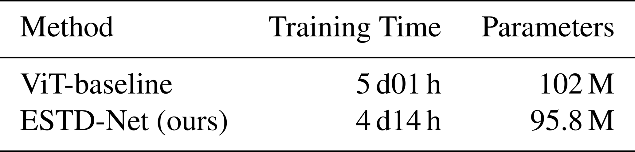
To evaluate the training efficiency of the proposed ESTD-Net, a comparison was conducted against a conventional Transformer-based model (ViT-baseline) under identical experimental settings, including dataset, GPU type, and optimizer configuration. The results, summarized in Table 7, indicate that ESTD-Net achieves faster training convergence while maintaining lower model complexity, demonstrating its computational efficiency relative to traditional Transformer architectures.

Table 7 Training time and model size comparison between ESTD-Net and ViT-baseline.

5 Conclusions

This paper presents ESTD-Net, a novel network architecture specifically designed for surface temperature data inpainting. Stage I employs an enhanced multi-head context attention mechanism within modified transformer blocks to effectively capture long-range pixel dependencies and improve boundary-aware reconstruction. Stage II utilizes a convolutional U-Net in an autoregressive manner to refine the coarse output from Stage I, enhancing local spatial continuity and smoothing boundaries, which is essential for producing coherent temperature fields. To further improve restoration fidelity, we integrate weighted reconstruction loss and gradient consistency regularization, ensuring that the inpainted results align with ground truth in both structural consistency and pixel-level accuracy.

While the results achieved using simulated data from the ERA5 reanalysis dataset demonstrate promising outcomes, real-world data introduces additional complexities. In practical applications, satellite observations are often incomplete, with certain regions consistently missing data due to factors such as cloud cover or sensor limitations. This inherent challenge results in a scarcity of fully complete surface temperature data. To address this issue, a practical approach involves extracting data from regions where observations are intact and artificially introducing gaps to simulate missing data for testing and evaluation purposes. This simulated dataset serves as a proxy for real-world conditions, enabling us to assess the model's robustness and performance within a more practical context.

By employing this method, we can further validate and fine-tune the reconstruction technique, ensuring its effectiveness in handling incomplete surface temperature data encountered in real-world applications. This approach provides a viable pathway for bridging the gap between idealized simulation-based testing and the complexities of real-world data, ensuring that ESTD-Net remains applicable across a wide range of environmental and climate research contexts.