A suite of coupled ocean-sea ice simulations examining the effect of regime shift in sea-ice thickness distribution on ice–ocean interaction in the Arctic Ocean

A major shift in Arctic sea ice occurred in 2007, transitioning from thicker, deformed ice to thinner, more uniform ice with reduced surface roughness. This abrupt change likely altered the dynamic and thermodynamic interactions between sea ice and ocean, with potential implications for nutrient and biogeochemical cycles in both sea ice and the upper ocean. In this study, we present a suite of regional coupled ocean-sea ice simulations designed to assess the potential impact of the regime shift on sea ice–ocean interactions, with a regional focus on the Atlantic sector of the Arctic Ocean. The different sea ice regimes are represented by changes in ice thickness distribution described by ice thickness classes in the sea ice model, and the effects of the different regimes are simulated through variations in the drag coefficient diagnosed from the ice thickness distribution. We emulate the two sea ice regimes by prescribing sea ice properties at the model's lateral boundaries. The results suggest a weaker dynamical coupling between sea ice and ocean in the new sea-ice regimes, leading to enhanced surface stratification, suppression of vertical mixing and momentum transfer to deeper layers. The simulation framework and the physical analyses presented here serve as a basis for ocean biogeochemical modelling studies that aim at understanding ocean ecosystem responses to changing Arctic sea ice.

1 Introduction

Sea ice regulates momentum, heat, and material exchanges between atmosphere and ocean in polar regions. It also supports biological production in and under the ice (e.g., Leu et al., 2015; Assmy et al., 2017). Large-scale sea ice properties, namely sea ice concentration and thickness, govern the details of these processes (Weeks, 2010). Lower ice concentration and thinner ice allow larger heat, gas and material exchanges, while higher ice concentration with thicker ice suppresses such processes (Fanning and Torres, 1991; Loose et al., 2009). Surface topography of sea ice, such as sails, keels, and melt ponds significantly modify momentum exchanges between atmosphere, ice and ocean (Cole et al., 2017; Brenner et al., 2021; Mchedlishvili et al., 2023), with significant consequences on the upper ocean processes including biogeochemical cycles (Long et al., 2012).

Ice thickness distribution (ITD) is a critical parameter for describing contributions from different types of sea ice on those processes (Tsamados et al., 2014; Martin et al., 2016; Sterlin et al., 2023). ITDs represent the amount of ice across different thickness classes within a given area. They can be derived from direct measurements of surface topography of sea ice. This is achieved by ice thickness measurements with short temporal and/or small spatial intervals, using e.g., altimeters or electro-magnetic sounding instruments (Haas et al., 2010; Farrell et al., 2011), or by upward-looking sonars on bottom-anchored moorings (e.g. Melling et al., 1995; Hansen et al., 2014). Modern sea ice models incorporate ITD as a sub-grid parameterization, allowing for explicit calculations of the combined effects of varying ice thickness on both dynamic and thermodynamic processes (Tsamados et al., 2014; Sterlin et al., 2023).

A major shift of ITD was observed in the Arctic Ocean in 2007 (Sumata et al., 2023). The shift was from thicker and deformed ice to thinner and more uniform ice regime. The fraction of very thick ice (e.g., exceeding 5 m) observed in Fram Strait was suddenly reduced by half, and has not recovered to date (Sumata et al., 2023; see also Fig. 1a). At the same time, the modal ice thickness, representing the thickness of the most frequently observed ice, dropped by approximately 1 m (Fig. 2b, the peak location of blue versus orange). The fraction of ice in the mode also increased (Fig. 2b, the peak height of blue versus orange), suggesting smoother ice. This is also suggested by Krumpen et al. (2025) based on airborne observations, with fewer and smaller ridges and reduced atmosphere–ice drag. These observed changes indicate that the ice floes after the shift are composed of a narrower range of thicknesses (less thickness variation and larger areal extent of flat level ice) with smaller sails and shallower keels (see Fig. 1b and c).

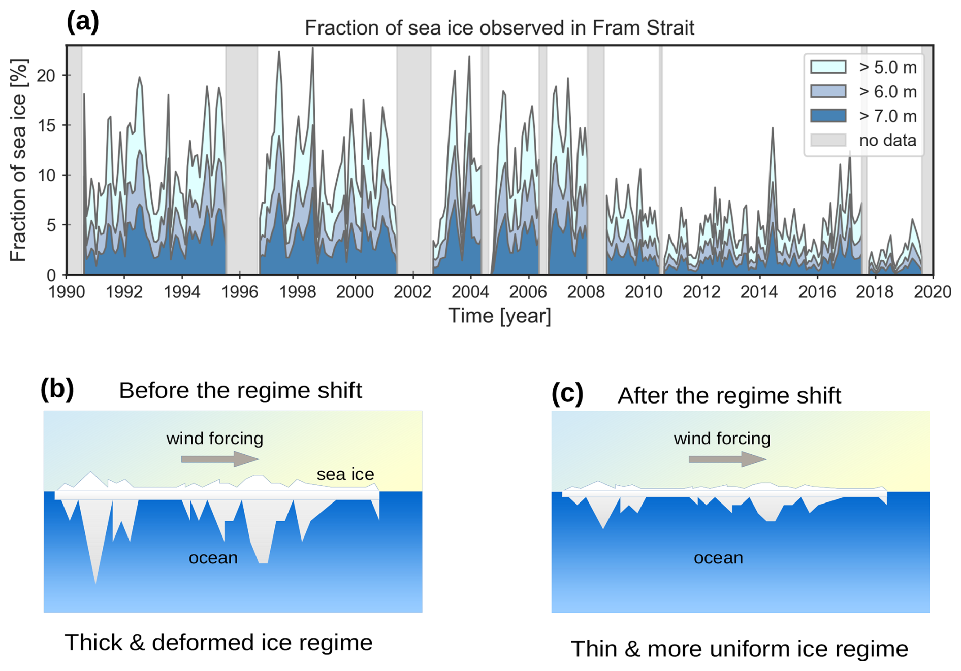
Figure 1 (a) Fraction of thick sea ice observed in Fram Strait, and (b, c) schematic illustration of contrasting different sea ice regimes. Panel (b) depicts the regime before the shift, characterized by thick ice with a larger fraction of heavily deformed ice. Panel (c) shows the regime after the shift, characterized by thinner, less deformed ice with a larger fraction of level ice. The time series in (a) is derived from sea ice draft data collected by upward-looking sonars moored in the western side of Fram Strait from 1990–2019 (The Fram Strait Arctic Outflow Observatory, see Data availability).

Such sudden, drastic changes in ITD are expected to have significant impacts on atmosphere–ice–ocean interactions and upper ocean processes. The thinner ice is mechanically weaker (Hibler, 1979; Feltham, 2008), allowing more frequent lead formation (Rheinlænder et al., 2024) and larger heat exchange (Landrum and Holland, 2022), and is prone to melting in summer. This may enhance the seasonal cycle of heat exchange between atmosphere and ocean through ice, and freshwater exchange between ice and ocean by enhanced melt-freeze cycle. The less deformed level sea ice, with smaller sails and shallower keels, has less dynamical interaction with the atmosphere and upper ocean (Cole et al., 2017; Brenner et al., 2021). Due to its smaller surface roughness, the ice after the regime shift is assumed to undergo a smaller drag force both from atmosphere and ocean. This may affect sea ice motion, while reducing momentum input from atmosphere to the ocean through ice, with possible consequences on upper ocean mixing and stratification.

These changes are arguably prominent in the Atlantic sector of the Arctic, where the Arctic-wide altered sea ice is advected from the central Arctic. A large fraction of sea ice in the central Arctic Ocean is initially formed in the surrounding marginal seas, e.g., Laptev, East Siberian, and Chukchi seas, and advected toward the Atlantic sector of the Arctic with time scales of 2–4 years (Sumata et al., 2023). Even sea ice formed in the Canada Basin is intermittently advected toward the Atlantic sector by the Transpolar Drift Stream (Hansen et al., 2014, Sumata et al., 2023) at a longer timescale. Thus, the Transpolar Drift integrates signals of changes occurring upstream in the Arctic and delivers them towards the Atlantic sector of the Arctic (Hansen et al., 2014; Krumpen et al., 2019).

Here we describe a suite of coupled ocean-sea ice simulations developed to investigate the possible consequences of the sea ice regime shift (particularly changes in the ice thickness distribution, ITD) on ice–ocean interaction and upper ocean processes. The simulations focus on the Atlantic sector of the central Arctic, specifically the downstream region of the Transpolar Drift Stream. To isolate the effects of the targeted processes, we employ a twin experiment approach, minimizing interference from other factors. The same experimental design is being applied in a separate future study to investigate the effects of the sea ice regime shift on upper ocean biogeochemistry, coupled to the same ocean and sea ice models used in this study. This work provides a detailed description of the physical component of the experiment and the resulting response of the physical environment. The paper is structured as follows; Sect. 2 provides a description of the model and the experimental design, Sect. 3 presents the results, and Sect. 4 provides concluding remarks.

2 Experimental design

2.1 Coupled sea ice – ocean model

We apply a regional setup of a coupled sea ice–ocean model for the numerical simulations. The sea ice component is the Los Alamos Sea Ice Model (CICE Ver. 5.1.2, Hunke et al., 2015) and the ocean component is the Regional Ocean Modeling System (ROMS Ver. 3.7, Shchepetkin and McWilliams, 2005). They are coupled by the Model Coupling Toolkit (MCT, Larson et al., 2005) in the METROMS framework (Debernard et al., 2021). This modeling configuration has been applied to a variety of studies with different regional setups (e.g., Idžanović et a., 2023, Röhrs et al., 2023). The current study employs a regional setup covering the Atlantic sector of the Arctic Ocean (Fig. 2a) with 4 km horizontal resolution, 35 vertical ocean layers, and 7 ice layers plus 1 snow layer, with 5 ice thickness classes. This specific regional setup has been developed and maintained at the Norwegian Polar Institute (Duarte et al., 2022).

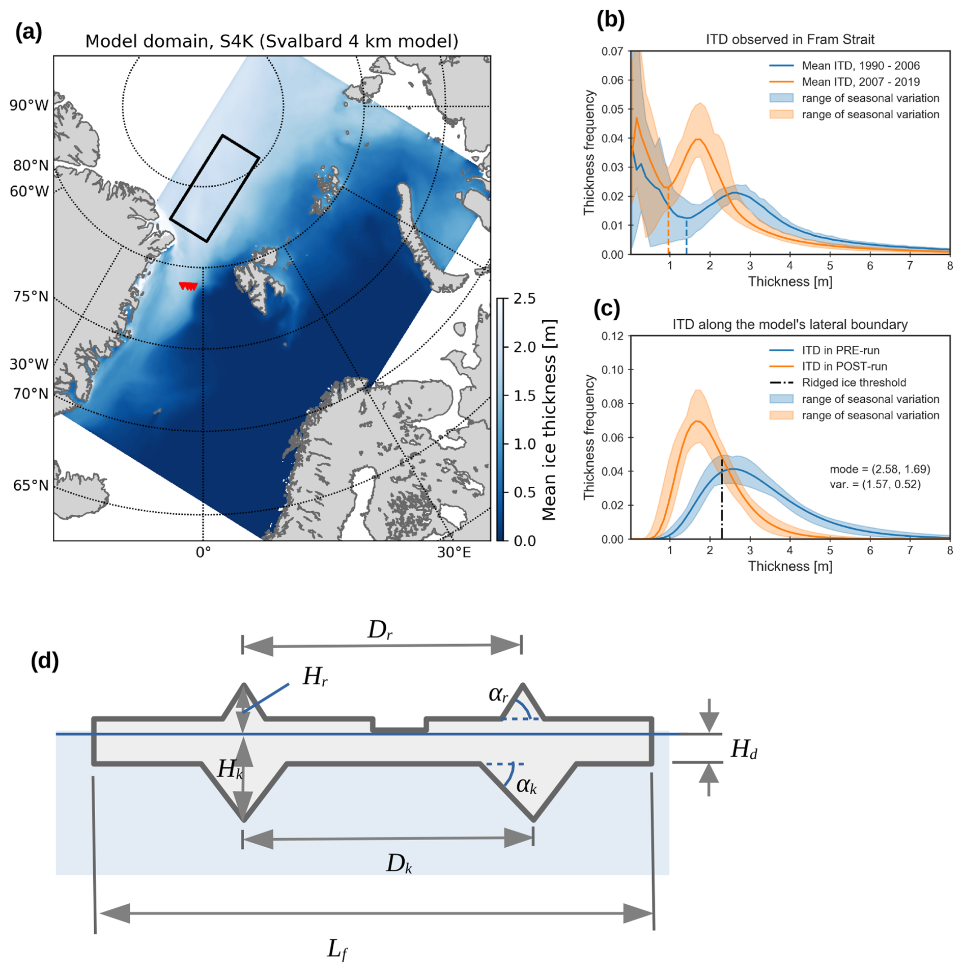
Figure 2 (a) Model domain; (b) mean sea ice thickness distribution observed in Fram Strait; (c) those prescribed at the lateral boundaries of the model domain; and (d) sketch of sea ice topography assumed in the form drag formulation (modified from Tsamados et al., 2014). The data acquisition areas in Fram Strait are indicated by red markers in panel (a). The solid black box in panel (a) denotes the focus area used in the Transpolar Drift analysis in Sect. 3.

The sea ice model describes ITD by discretized ice thickness classes and calculates contributions from different ice classes on dynamic and thermodynamic processes (Hunke et al., 2015). In each ice thickness class, the ice is further divided into two sub-categories, flat level ice and deformed ridged ice. The former ice has less contribution to the drag force at the interfaces while the latter has a larger and significant contribution as described below. Transfer of sea ice volume between ice classes and categories is governed by thermodynamic (e.g., melting, freezing) and dynamic (e.g., ridging) processes in the model. The model describes momentum transfer between atmosphere, sea ice and ocean by a quadratic bulk formula with a variable drag coefficient. The drag coefficient varies in space and time and takes into account effects of time-evolving surface roughness of sea ice (form drag formulation, Tsamados et al., 2014). This formulation comprises an important part of the current experiment design, as the variable drag coefficient is diagnosed from the areal and volume fraction of ice in the ice thickness classes and categories, which represents the two different ice regimes in the simulation.

2.2 Variable drag coefficient

The form drag formulation computes the neutral drag coefficient between sea ice and ocean as:

$$\begin{array}{}\text{(1)}& C_{\mathrm{d}}=C_{\text{keel}}+C_{\text{floe}}+C_{\text{skin}}\end{array}$$

where C_keel, C_floe, and C_skin represent contributions from ice keels, floe edges, and surface skin drag, respectively. The drag coefficient between sea ice and atmosphere also has the same formula, with an additional contribution from melt pond edges. Although the form drag formulation is applied at both the ice–ocean and ice–atmosphere interfaces, we focus here on the ice–ocean interface to avoid redundancy (the differences being the inclusion of melt pond edges and the use of distinct parameter values). Following Tsamados et al. (2014), the contributions from ice keels, floe edges and skin drag are formulated as a function of surface topography of sea ice (Fig. 2d). The essence of modeling the variable drag coefficient is to relate prognostic variables in the model (e.g., volume fraction of ridged ice in a grid cell) to the drag coefficient, with simplified assumptions on the mean shape of topographic features of ice (e.g., ridges and keels).

The contribution from keels is given by a function of ice concentration, A, the mean keel depth, H_k, and the mean distance between keels, D_k, as follows (see also Fig. 2d),

$$\begin{array}{}\text{(2)}& C_{\text{keel}}={\displaystyle \frac{\mathrm{1}}{\mathrm{2}}}{c}_{\mathrm{k}}A{\displaystyle \frac{H_{\mathrm{k}}}{D_{\mathrm{k}}}}{S}_{\mathrm{k}}^{\mathrm{2}}{P}_{\mathrm{k}},\end{array}$$

where c_k is the local resistance of a keel, S_k represents sheltering effect by a keel (given by a function of ridging intensity, $H_{\mathrm{k}}/D_{\mathrm{k}}$), and P_k represents integrated effect of boundary layer on the keel drag (see Table 1 for details and a summary of notation). The contribution from floe edges is similarly formulated as a function of ice concentration, A, ice draft, H_d, and the mean floe length, L_f, as

$$\begin{array}{}\text{(3)}& C_{\text{floe}}={\displaystyle \frac{\mathrm{1}}{\mathrm{2}}}{c}_{\mathrm{f}}A{\displaystyle \frac{H_{\mathrm{d}}}{L_{\mathrm{f}}}}{S}_{\mathrm{f}}^{\mathrm{2}}{P}_{\mathrm{d}}.\end{array}$$

where c_f is the local resistance at floe edges, S_f represents sheltering effect by floe edges (Lüpkes et al., 2012), and P_d represents integrated effect of boundary layer on the floe edge drag. The contribution from the skin drag with a presence of ice keels is given as follows,

$$\begin{array}{}\text{(4)}& C_{\text{skin}}=c_{\mathrm{s}}\left(\mathrm{1}-m_w{\displaystyle \frac{H_{\mathrm{k}}}{D_{\mathrm{k}}}}\right),\end{array}$$

where c_s is the local skin drag coefficient and m_w is the attenuation parameter for skin drag. The above Eqs. (2–4) relate drag coefficients to the topographic parameters of sea ice (e.g., H_k, D_k, L_f) in each grid cell. The topographic parameters are diagnosed from the prognostic variables in the sea ice model: sea ice concentration, A, areal fraction of ridged ice, a_rdg, and volume fraction of ridged ice, v_rdg,

$$\begin{array}{}\text{(5)}& {\displaystyle }& {\displaystyle }{H}_{\mathrm{k}}=\mathrm{2}{\displaystyle \frac{v_{\text{rdg}}}{a_{\text{rdg}}}}{\mathit{\psi }}_{\mathrm{s}},\text{(6)}& {\displaystyle }& {\displaystyle }{D}_{\mathrm{k}}=\mathrm{2}{H}_{\mathrm{k}}{\displaystyle \frac{A}{a_{\text{rdg}}}}{\mathit{\psi }}_{\mathit{\theta }},\text{(7)}& {\displaystyle }& {\displaystyle }{L}_{\mathrm{f}}=L_{\text{min}}{\left({\displaystyle \frac{A_{*}}{A_{*}-A}}\right)}^{\frac{\mathrm{1}}{\mathrm{2}}},\end{array}$$

where ψ_s and ψ_θ are fixed parameters describing the mean shape of the keels (Table 1), L_min is a prescribed minimum floe length, and A_∗ is a number close to but slightly larger than 1 introduced to avoid singularity of L_f when A∼1. These quantities are diagnosed in each grid cell after summing up areal and volume fraction of ridged ice in all ice thickness classes. Therefore, temporal evolution of ITD including fraction of ridged ice changes the modeled drag coefficient by changing topographic parameters of sea ice, H_k, D_k, H_d, and L_f. In the following Section, we describe how we prescribe the prognostic sea ice variables along the model's lateral boundaries to set up the twin experiments.

Table 1 List of variables used in the form drag formulation.

2.3 A suite of twin experiments

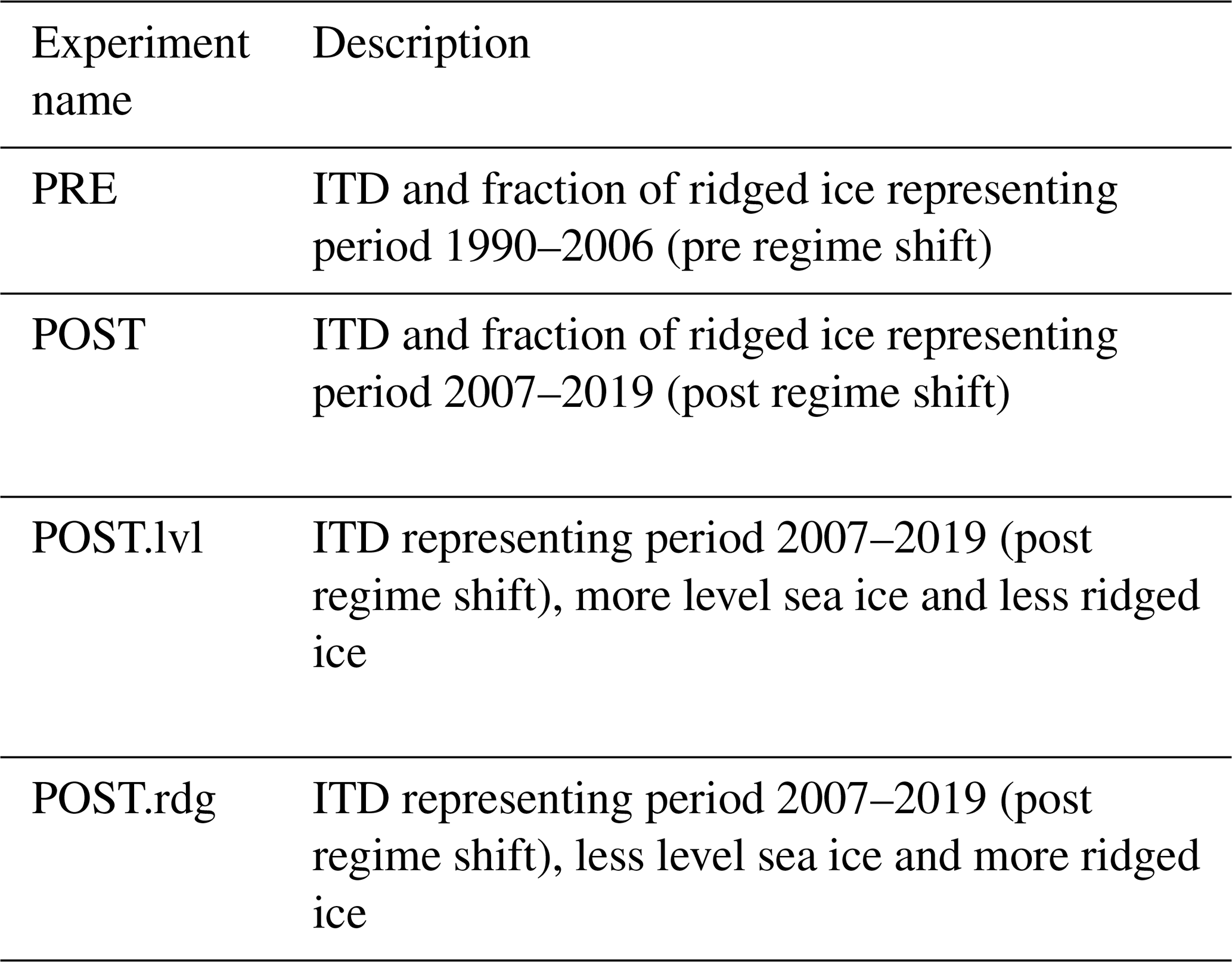
We set up twin experiments with two distinctive sea ice regimes. One represents the thick and deformed ice regime before 2007 (hereafter called PRE-run), while the other represents thin and more uniform ice regime after 2007 (hereafter POST-run). We define the two regimes through idealized ITDs (Fig. 2c), based on those observed in Fram Strait (Sumata et al., 2023; see Fig. 2b). The ITDs are prescribed along the model's lateral boundaries (Sumata et al., 2025). Since the large fraction of sea ice in the model domain is advected from the central Arctic by the Transpolar Drift, the domain is filled with sea ice coming from the model's northern and eastern boundary with a time lag shorter than one year. This setup enables us to prescribe sea ice conditions inside the model domain by those along the boundaries, without manipulating sea ice inside the domain.

The idealized ITDs shown in Fig. 2c are derived from a least-squares fit of the observed ITDs for the two periods (Fig. 2b) to lognormal distributions. The fraction of thin ice observed in Fram Strait was excluded by a cut off threshold at the minimum frequency of the bi-modal thickness distributions (dashed lines in Fig. 2b). This approach removes the fraction of new and young thin ice formed in the vicinity of Fram Strait locally, and enables us to provide approximate ITDs for the central Arctic (see, e.g., Rabenstein et al., 2010, von Albedyll et al., 2021). The fit is applied for monthly ITDs for both PRE-run and POST-run. The fraction of ridged ice is defined by a fixed thickness threshold of 2.3 m (dot-dashed line in Fig. 2c). All the ice thinner than the threshold is categorized as level ice, while thicker ice is categorized as ridged ice in both cases. The ITDs shown in Fig. 2c with the distinction between level and ridged ice are remapped to the model's ice thickness classes and given as the lateral boundary condition for each run.

We apply the same initial conditions, ocean boundary conditions and surface atmospheric forcing in both runs. Only the lateral boundary condition for ITD differs between the two runs. The initial conditions for the ocean are given by the Pan-Arctic 4 km model (A4 model, Hattermann et al., 2016), while the simulations start from no-ice condition. The latter is to assure filling the model domain by sea ice with the ITDs prescribed at the lateral boundaries. The lateral boundaries of the model ocean are forced by the A4 model, while those of sea ice (other than the prescribed ITD) are forced by the reanalysis field from TOPAZ4 data assimilation system (Sakov et al., 2012, Xie et al., 2017). The model is driven by ERA5 atmospheric reanalysis field (Hersbach et al., 2020), from 2012–2015. The short simulation window (4 years) is employed to preserve the similarity of the background ocean stratification under the Arctic halocline in the twin experiments. The last 3 years (2013–2015) are used for the analyses. The background ocean conditions in shallow levels, i.e., those in seasonal mixed layer and in upper halocline, are expectably affected by changing ice–ocean interactions and will thus differ between the simulations. These differences are analysed in our study.

An additional set of sensitivity experiments are also conducted to examine the interplay between dynamical ice–ocean coupling and changes in buoyancy flux in the upper ocean. In these sensitivity experiments, we use the same ice thickness distribution (ITD) representing the condition after the regime shift (POST), but with different fractions of ridged ice. These experiments are referred to as the POST.rdg and POST.lvl runs (see Table 2). The POST.rdg run represents a ridged ice regime, using the ITD from POST with a thickness threshold of 1.9 m to define ridged ice. This results in a higher fraction of ridged ice compared to the POST run, while maintaining the same mean ice thickness. In contrast, the POST.lvl run represents a level ice regime, applying the same ITD (POST) but using a threshold of 3.1 m. This setup increases the fraction of level ice relative to the POST run though the mean ice thickness is unchanged. All other model configurations, i.e., the initial ocean and ice conditions, lateral ocean boundary conditions, and surface atmospheric forcing, are identical to those in the PRE and POST runs. This setup ensures that the surface buoyancy forcing remains the same (as sea ice concentration and mean ice thickness are unchanged) while modifying the dynamical coupling through different ice–ocean drag coefficients, and enables us to isolate the effect of changes in dynamical coupling.

Table 2 List of the twin and sensitivity experiments.

3 Physical environment simulated in the twin experiments

3.1 Changes in sea ice and momentum transfer

The twin experiments successfully reproduced two distinct sea ice regimes in the Atlantic sector of the Arctic. The mean ice thickness in the perennial ice-covered area was reduced by approximately 1 m in the POST-run (Fig. 3a and b, similar results in summer, Fig. S1 in the Supplement), while changes in ice concentration were limited to the marginal ice zone (Fig. 3c, see also Fig. S1). The volume of ridged ice (V_rdg) and ridging intensity ($H_{\mathrm{k}}/D_{\mathrm{k}}$) also decreased in POST-run (Fig. 3d and e), consistent with the prescribed boundary conditions. The reduced ridging intensity lowered the effect of keel drag, which, consequently, led to a smaller total drag coefficient (Fig. 3f, see also Fig. S2 in the Supplement). The effects of other drag terms were generally small: contributions from floe edge were limited in summer to less than 30 % at maximum, and the skin drag was more than one order of magnitude smaller than other terms.

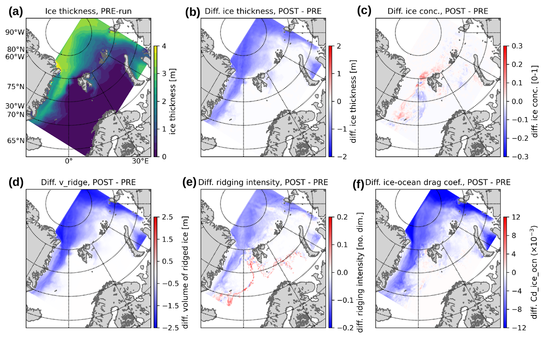
Figure 3 Spatial pattern of simulated sea ice properties and their difference between POST and PRE runs (POST–PRE): (a) Mean ice thickness in PRE run. Differences of mean (b) ice thickness, (c) ice concentration, (d) volume of ridged ice, shown as volume per unit area [m], (e) ridging intensity, and (f) total ice–ocean drag coefficient. All the panels show winter months average (from January–March).

The reduction of both atmosphere–ice and ice–ocean drag coefficient decreased momentum exchange between atmosphere, ice and ocean (Fig. 4a and d), leading to different effects on ice drift speed during winter and summer. In winter, the reduced drag caused faster ice motion (Fig. 4b), whereas in summer, it resulted in slower ice motion (Fig. 4c). During winter, sea ice in the Atlantic sector is primarily driven by strong northerly winds, with ocean drag acting as a retarding force that slows ice drift (Fig. 4d, November–April). In the POST-run, the reduction of ice–ocean drag weakened this retarding force on the ice drift with the Transpolar Drift, allowing the ice to move faster. In summer, however, significant wind forcing is absent (Fig. 4d, June–October), and the southward ice motion in this region is primarily driven by ocean surface currents. The weaker drag in the POST-run reduced the driving force for this southward ice motion, resulting in slower ice drift. Note that the ratio between the two drag coefficients, ice–ocean and atmosphere–ice, differs between the PRE-run and POST-run. The reduction of the total drag coefficient is more prominent in ice–ocean drag compared with atmosphere–ice drag in the POST-run (Material S3–S5 in the Supplement), resulting in a more wind-driven regime after the regime shift.

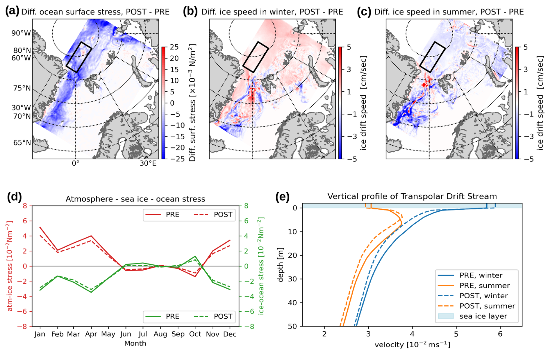
Figure 4 Differences between PRE and POST runs of (a) ocean surface stress, (b) ice velocity in winter, (c) ice velocity in summer, (d) atmosphere–ice–ocean stress, and (e) vertical velocity profile of the ice and upper ocean in the Transpolar Drift. Panel (a) shows the difference in annual mean surface stress. In panels (b), (c), (e), winter refers to the period from January–March, summer refers to June–August. The solid-black rectangular box in panels (a)–(c) outlines the region of the Transpolar Drift analyzed in panels (d), (e). Panel (d) shows the stress component along the major axis of this box; positive values indicate a stress toward the Eastern coast of Greenland. The values are averaged over the boxed area. Panel (e) shows the vertical velocity profile of the Transpolar Drift averaged over the boxed region. Positive values are defined similarly as in panel (d). The uppermost light-blue shading in (e) represents sea ice.

The smaller momentum exchange in the POST-run reduced the dynamical coupling between sea ice and ocean and affected surface ocean currents. In winter (Fig. 4e, blue lines), ice moves faster than ocean surface currents and ocean currents decrease rapidly with depth. The smaller drag in POST-run resulted in faster ice motion and slower ocean current compared to PRE-run (Fig. 4e, blue dashed line versus blue solid line). In summer, ocean surface currents are faster than ice drift in both runs (Fig. 4e, orange lines). It has a maximum in the surface layer (<10 m depth) and slows down upward, indicating that the ocean current drives ice. The weaker drag in POST-run makes the difference between ice motion and surface ocean current large, enabling the ocean to develop shallower velocity maximum than in PRE-run. Additionally, the POST-run showed a more sharp decline of the ocean currents with depth both in summer and winter (Fig. 4e, dashed lines versus solid lines), indicating weaker downward momentum transfer and a spin-down of the ocean circulation under ice.

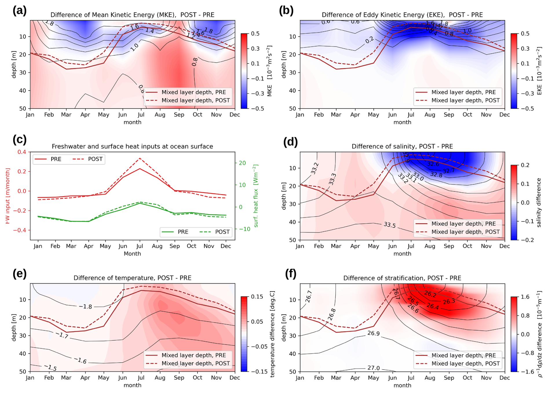
Figure 5 Differences in ocean properties between the PRE and POST runs within the transpolar drift region: (a) Mean Kinetic Energy, (b) Eddy Kinetic Energy, (c) freshwater flux and surface heat flux, (d) salinity, (e) temperature, and (f) stratification. All values are averaged over the boxed area shown in Fig. 2a. In panels (a), (b), (d), (e), black contours represent values from the PRE-run, while colors indicate differences between the two runs. In panel (f), contours depict density from the PRE-run, and colors represent changes in stratification between the two runs. The magenta lines in panels (a), (b), (d)–(f) indicate the mixed layer depth, defined as the depth at which the local density exceeds the surface density by 0.03 kg m⁻³, following de Boyer Montégut et al. (2004).

3.2 Changes in upper ocean

The weaker dynamical coupling in the POST-run made the upper ocean (<20 m) less energetic. The less momentum transfer between ice and ocean in POST-run resulted in reduction of both mean and eddy kinetic energy (hereafter MKE and EKE) in the upper ocean, roughly in the depth range of the mixed layer (Fig. 5a and b). Here we divided the mean and eddy fluctuations by a 30 d temporal filtering, i.e.,

$$\begin{array}{}\text{(8)}& \text{MKE}={\displaystyle \frac{{\overline{u}}^{\mathrm{2}}+{\overline{v}}^{\mathrm{2}}}{\mathrm{2}}},\end{array}$$

where $\overline{u}$ and $\overline{v}$ are the 30 d low-pass filtered u and v, while

$$\begin{array}{}\text{(9)}& \text{EKE}={\displaystyle \frac{(u^{\prime \mathrm{2}}+v^{\prime \mathrm{2}})}{\mathrm{2}}},\end{array}$$

where u^′ and v^′ are the 30 d high-pass filtered velocity (a Fourier/Spectral filtering is applied). Note that the Rossby's deformation radius in our study area is comparable to or smaller than our 4 km-horizontal resolution, indicating that the EKE could be underestimated. MKE in the shallow part of the ocean (<20 m) exhibits a strong seasonal cycle (shown by black thin contour in Fig. 5a); MKE is large in winter and small in summer. In POST-run, the reduction of MKE was evident in winter, while a slight increase occurred in summer (color shade in Fig. 5a), indicating that the seasonal cycle of MKE became weaker in POST-run as a consequence of the weaker dynamical coupling. In contrast to MKE, EKE is large in summer (black thin contours in Fig. 5b). In summer, ice is thin, weakly connected laterally, and vulnerable to deformation. The fragile ice condition in summer gives rise to spatially incoherent, nonuniform momentum exchange between ice and ocean. This developed mesoscale and short-timescale fluctuations of ocean current just underneath the ice cover (see e.g., Fig. S6 in the Supplement). Such fluctuations, represented by EKE, also reduced in POST-run (color shade in Fig. 5b) as a consequence of the weaker dynamical coupling.

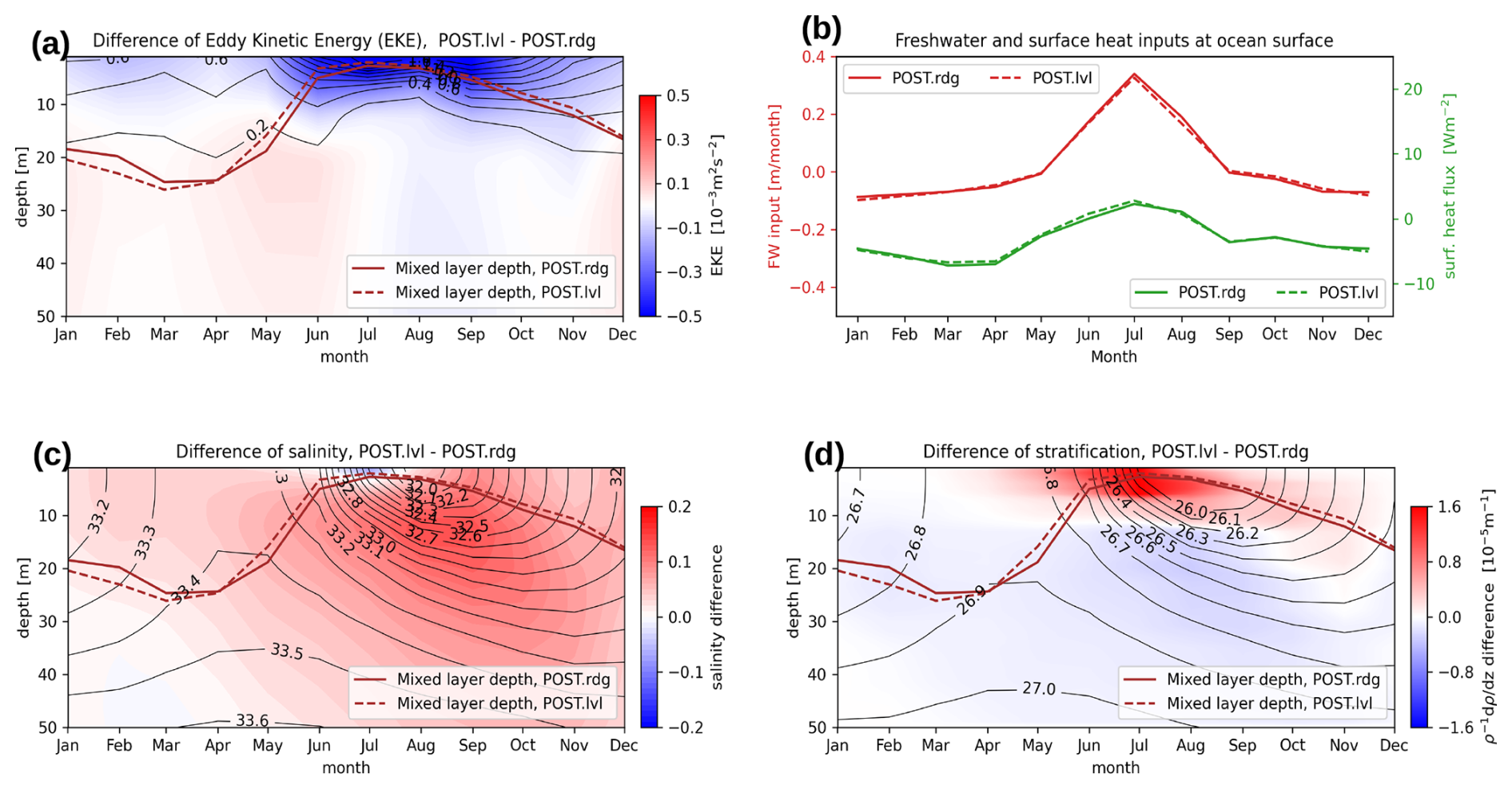
Figure 6 Differences in ocean properties between POST.rdg and POST.lvl runs within the transpolar drift region: (a) Eddy Kinetic Energy, (b) freshwater flux and surface heat flux, (c) salinity, (d) stratification. All values are averaged over the boxed area shown in Fig. 2a. In panels (a), (c), (d), black contours show values from the POST.rdg run, while colors indicate differences between the two runs. In panel (d), contours depict density from the POST.rdg run, and colors represent changes in stratification between the two runs.

The weaker MKE and EKE in POST-run, together with changes in surface buoyancy fluxes, made the upper ocean more stratified and the mixed layer shallower. Due to the thinner modal ice thickness and weaker ice strength (Fig. S7 in the Supplement), sea ice in POST-run is more prone to melting and mechanical fracture in summer. This enhances the seasonal cycle of heat and freshwater exchanges between ice and ocean (Fig. 5c). Though the changes in surface heat flux are small (green lines in Fig. 5c), the freshwater flux exhibited distinct changes; enhanced meltwater input to the upper ocean in summer and enhanced freshwater extraction due to freezing in winter (red lines in Fig. 5c). The increase of the freshwater input in summer made the surface ocean less saline (blue shade in Fig. 5d), while the increase of freshwater extraction in winter made the surface ocean slightly more saline (red shade in Fig. 5d). As a consequence, POST-run exhibited an enhanced seasonal cycle of ocean surface salinity. Together with the suppressed mixing (Fig. S8 in the Supplement) associated with the smaller MKE and EKE (Fig. 5a and b), the changes in freshwater exchange made the surface ocean more stratified and shoals the mixed layer in POST-run (magenta lines in Fig. 5d, e and f).

A set of additional sensitivity experiments underscores the significant role of the interplay between dynamical coupling and buoyancy flux in capturing the integrated effect. In the sensitivity experiments (POST.lvl versus POST.rdg, see Table 2), the same buoyancy flux was applied at the ocean surface while only the dynamical coupling was altered. This was enabled by applying the same ice thickness distribution while differing fraction of ridged ice. The results again demonstrated a reduction in EKE (Fig. 6a) and weaker surface mixing under weaker dynamical coupling (Fig. S9 in the Supplement). However, due to negligible changes in freshwater flux between the runs (Fig. 6b), surface freshening was absent (Figs. 6c vs. 5d) and changes in mixed layer depth were not visible (Fig. 6a magenta lines). The weaker mixing led to increased stratification near the ocean surface, particularly during summer (Fig. 6d), reflecting the absence of additional freshwater forcing at the surface (Figs. 6b vs. 5c). These findings emphasize the necessity of simultaneously considering dynamic and thermodynamic changes in sea ice to fully understand their impact on the upper ocean.

Note that the additional experiment also enables us to disentangle the effect of the changing drag and ice strength. POST.lvl shows a significant reduction in the ice–ocean drag coefficient (Fig. S10 in the Supplement), associated with the reduced fraction of ridged ice, while sea-ice strength is nearly the same (Fig. S11 in the Supplement). The resulting changes (POST.rdg vs. POST.lvl) reproduce the characteristic features observed in the comparison between PRE and POST, i.e., ice drift acceleration in winter, ice drift deceleration in summer, and more decoupling between ice drift speed and ocean current under ice (Fig. S9). These results indicate that the features highlighted in the PRE vs. POST comparison are primarily driven by changes in ice–ocean drag coefficient, while contributions from changes in ice strength likely play only a secondary role.

4 Concluding remarks

We set up a suite of coupled sea ice–ocean simulations to examine the potential impact of the sea ice regime shift (Sumata et al., 2023), with a focus on the effect of thinner and less deformed sea ice on ice–ocean interactions in the Atlantic sector of the Arctic. After 2007 the ice is thinner and less deformed, characterized by two notable changes from earlier, namely lower mean ice thickness with a higher fraction of ice in the modal category, and a reduction in surface roughness. These sea ice features were prescribed by different ice thickness distribution along the lateral boundaries of the model domain, and we emulate the two distinctive sea ice regimes before and after the shift. Based on these experiments, we describe the apparent responses, with a focus on sea ice–ocean interaction and upper ocean processes in the perennial ice-covered area.

Our experiments suggest that the thinner and smoother ice enhances freshwater exchange between ice and ocean, as this type of ice is mechanically weaker and more sensitive to thermal forcing. This leads to increased ice melt during summer and more ice formation in winter, amplifying the seasonal variability in surface salinity. This strengthens upper ocean stratification during summer and reduces the mixed layer depth. The decrease in surface roughness, on the other hand, lowers the drag both at the ice–ocean and ice–atmosphere interfaces, weakening the dynamical coupling between them. In winter, this enables faster sea ice drift under the same wind forcing, whereas in summer, it decelerates ice motion driven by ocean currents. The weakened dynamical coupling also decouples ocean surface currents from ice motion, resulting in reduced kinetic energy in both mean and eddy currents especially in the mixed layer. Consequently, vertical mixing is suppressed, momentum transfer to deeper layers is reduced, and the upper ocean becomes more stratified with thinner and less deformed ice. The decrease in ice–ocean coupling in the post regime-shift simulations is consistent with results regarding the long-term decline in ocean surface stress in ice-covered areas of the Arctic (e.g. Martin et al., 2016; Sterlin et al., 2023), whereas it contradicts results obtained from models with constant drag, where the increase in ice drift speed leads to increasing ocean surface stress in CMIP6 models (Muilwijk et al., 2024).

Regarding the ocean biogeochemical cycle, our result suggests that the sea-ice regime shift could cause a decrease of nutrient exchanges across the mixed layer in sea-ice covered areas, through an interplay with other concurrent factors needs further examination. The follow-up of this study will use a similar experimental design but including ocean biogeochemistry and, at a later stage, also sea ice biogeochemical cycles in the simulations to get insight into the consequences of the sea-ice regime shift on primary production.

Note that this study specifically addresses one aspect of the ongoing changes in sea ice–ocean processes in the Atlantic sector of the Arctic, without attempting to encompass the full spectrum of influencing factors. It does not incorporate changes in wind forcing (Ward and Tandon, 2024; Muilwijk et al., 2024), retreat of sea ice cover (Serreze et al., 2007; Fox-Kemper et al., 2021), increased ocean heat content in adjacent marginal seas (Timmermans, 2015; Lind et al., 2018; Muramatsu et al., 2025), or modifications in large-scale ocean circulation and stratification (Polyakov et al., 2017, 2020). Given the simultaneous occurrence and interaction of these factors, isolating a single process allows for a more detailed examination of the dynamics within this complex system. Further investigations are necessary to examine effects of other key factors and their interplay, in parallel to improvement of key processes of ice–ocean interactions, such as parameterizations of ice topography and ice–ocean coupling.