Evaluation of coupled and uncoupled ocean–ice–atmosphere simulations using icon-2024.07 and NEMOv4.2.0 for the EURO-CORDEX domain

Evaluation results from the reanalysis-driven (ERA5/ORAS5) simulation for the years 1979–2021 with a regional coupled ocean–atmosphere model (ROAM) are presented. The coupled setup portrayed here is one of the first regional climate modeling systems to couple the ICON atmosphere model in climate limited-area mode (CLM) with the ocean model NEMO for the North and Baltic Sea (NBS), using a flux-based OASIS3-MCT coupling approach. Along with the simulation using the coupled model configuration ROAM-NBS, the simulations with the uncoupled components (ICON-CLM and NEMO-NBS, respectively) are analyzed and compared with various observational datasets. ROAM-NBS complements atmosphere-only climate projections with the same atmospheric model and setup, which will all be published in accordance with EURO-CORDEX specifications. Climate projections by ROAM-NBS will enrich the data available to support the German Strategy for Adaptation to Climate Change (DAS), especially for our target region, which are the German national waters.

In general, the mean model climate is well represented by all setups. The sea surface temperature (SST) bias is, on average, about ±0.5 K. Differences in fluxes and precipitation over the ocean between the coupled and uncoupled simulations are largely related to SST differences. However, the mean influence on the land areas is negligible. The evaluations of ocean variables indicate a strong agreement between ROAM-NBS and NEMO-NBS. Compared to observations, both simulations overestimate sea ice concentration and extent. Mean temperature and salinity profiles in the Baltic Sea are generally reproduced by both simulations, with biases in the deeper layers. Major inflow events are captured but underestimated. Sea surface height and storm surge highly coincide with observational data, with NEMO-NBS slightly outperforming ROAM-NBS in terms of correlation. The marine heat wave (MHW) evaluation against observations in the North and Baltic Sea demonstrates that the simulations capture the inter-annual variability of MHW characteristics.

Overall, the coupled simulation demonstrates adequate performance for both the atmosphere and the ocean, and the setup will be used to produce coupled regional climate projections for Europe. However, bias correction for the deeper Baltic layers remains necessary for further applications, and future work will focus on refining the setup for this region.

1 Introduction

In climate modeling and research, the results of regional coupled or ocean models are still underrepresented compared to global ones. While the regional downscaling of the atmosphere is coordinated through the CORDEX initiative (Giorgi et al., 2009), data from regional ocean models remain sparse. Only in 2025, the CORDEX Task Force on Regional Ocean Climate Projections (https://cordex.org/strategic-activities/taskforces/task-force-on-regional-ocean-climate-projections; last access: 25 September 2025) was established. Since standalone ocean models are ideally forced by the output of regional atmospheric models, the ocean simulations can only be delivered with a considerable delay compared to the global climate simulations due to the downscaling chain. Thus, one advantage of using a regional coupled ocean–atmosphere model for climate projections, compared to the stand-alone ocean component, is the independence of regional climate model (RCM) projections from CMIP6. Moreover, the regional coupled model allows us to deliver consistent information on climate and climate change for the atmosphere and the ocean in the North and Baltic Sea (NBS) region, with a particular focus on the German coasts. For the Baltic Sea region, a number of investigations using regional coupled models were conducted within the framework of Baltic Earth (https://baltic.earth, last access: 9 July 2025). Gröger et al. (2021) review progress on coupled modeling in that context. The investigations considered in the review outline different aspects of the added value of regional coupled models. Gröger et al. (2021) summarize that only online coupled high-resolution ocean models can represent small-scale ocean processes accurately. They also conclude that the demonstration of the added value of coupled models over their uncoupled counterparts is often influenced by biases in datasets, such as runoff, used for the forcing of the uncoupled versions. Christensen et al. (2022) analyzed RCM projections with and without ocean coupling, forced by global climate model (GCM) simulations provided with the fifth phase of the coupled model intercomparison project (CMIP5). Their focus was on climate change in the Baltic Sea region. They showed that the coupled simulations can exhibit differences in future sea surface temperatures and sea ice conditions compared to the respective uncoupled versions, which can locally modify the climate change signal.

As shown by Gröger et al. (2021), different regional coupled ocean–atmosphere models have been in use for the NBS region. These are coupled versions of CCLM and NEMO (e.g. Pham et al., 2014; Primo et al., 2019; Ho-Hagemann et al., 2020), RCA4 and NEMO (Gröger et al., 2015; Dieterich et al., 2019), REMO and MPIOM (Sein et al., 2015), or Hirham and HBM (Tian et al., 2013). Karsten et al. (2024) present a recent development of a coupled ocean–atmosphere model, which couples the atmosphere and the ocean component (CCLM and MOM5, respectively) via an exchange grid. Bauer et al. (2021) were coupling ICON and GETM via an ESMF exchange grid. However, the ocean domains of their coupled models only encompass the Baltic Sea, or an even smaller domain in the case of Bauer et al. (2021), which is merely a small part of the whole EURO-CORDEX domain used for the atmosphere. A first version of a coupled regional ocean–atmosphere model incorporating ICON in climate limited-area mode (ICON-CLM) and NEMO was presented by Ho-Hagemann et al. (2024). The modeling system is called GCOAST-AHOI, just as its earlier version (Ho-Hagemann et al., 2020). Ho-Hagemann et al. (2024) found that the new version of GCOAST-AHOI could well capture near-surface air temperature, precipitation, mean sea level pressure, and wind speed at a height of 10 m. However, there was a prevailing negative sea surface temperature (SST) bias of 1–2 K, which they attributed to an underestimation of the downward shortwave radiation at the surface.

Here, we introduce ROAM-NBS, a new version of a regional coupled ocean–ice–atmosphere modeling system covering the full EURO-CORDEX domain for the atmosphere and the North and Baltic Sea for the ocean. ROAM-NBS combines the ICON-CLM atmosphere model (version icon-2024.07) with the NEMOv4.2.0 ocean model and the Sea Ice modelling Integrated Initiative (SI3) thermodynamic sea ice model, coupled via OASIS3-MCT using a flux-based exchange approach. Compared to the version by Ho-Hagemann et al. (2024), ROAM-NBS is based on a later NEMO version and includes a new ocean bathymetry, which is specifically designed for a good representation of the German coastline. Moreover, our setup also integrates a refined treatment of radiation in NEMO based on prescribed chlorophyll distributions, supporting a realistic representation of shallow and stratified shelf seas. With the use of a later ICON release, a more recent NEMO version with major updates, higher-resolution coastal bathymetry, and enhanced representation of surface fluxes and radiation, ROAM-NBS represents a methodological advance over previous GCOAST configurations.

Using ROAM-NBS and different configurations of GCOAST-AHOI described by Ho-Hagemann et al. (2020, 2024), which all employ an online coupled ocean for the NBS region, CMIP6 climate projections will be downscaled for the EURO-CORDEX region (Jacob et al., 2014). These coupled regional climate projections will complement the RCM simulations of CORDEX-CMIP6 (https://github.com/WCRP-CORDEX; last access: 23 May 2025). The simulation status is updated regularly and can be viewed at https://wcrp-cordex.github.io/simulation-status/CORDEX_CMIP6_status.html#EUR-12 (last access: 23 May 2025). The evaluation simulation analyzed in this article defines the setup of ROAM-NBS that will be used for downscaling. In addition to publishing the data on the ESGF nodes within the EURO-CORDEX community, ROAM-NBS will be applied to generate an ensemble of climate projections that can be used for climate adaptation measures in German national waters. Related evaluations will be published on https://das.bsh.de (last access: 9 July 2025).

The comparison of coupled simulations against their uncoupled counterparts, which are forced by high-quality reanalyses like ERA5 (Hersbach et al., 2020) at the ocean–atmosphere interface, can never be a fair one. Thus, the most important added value of using a regional coupled model for climate projections is not shown when evaluating the reanalyses-driven evaluation simulation, where we can provide good forcing data for both components for uncoupled simulations. The added value can rather be shown in the next step, when we generate the coupled regional historical simulations (i.e., for the historical time period as the reanalysis-driven evaluation simulation, but with GCM data as lateral boundary conditions) and the climate projections, which are not part of this article. However, even if the added value of coupling cannot be fully quantified from reanalysis-driven simulations, the evaluation provides an essential test of consistency and robustness.

The main aim of this article is to analyze the general performance of the coupled evaluation simulation, considering the atmosphere, the ocean, and the sea ice components.

We evaluate whether the coupling leads to any significant degradation or drift in mean climate and whether major climate-relevant features such as SSTs, near-surface air temperature, surface heat fluxes, stratification, and extreme sea level are consistently represented. Therefore, we are comparing the individual components against measurement data, as well as the coupled simulation against the simulations of the standalone versions of the atmosphere and the ocean–sea-ice component. As each component can introduce new biases into the system, it has to be ensured that the coupled system yields comparable results to those of the individual components.

After providing an overview of the coupled system and its individual components in Sect. 2, the evaluation is presented in two parts: in Sect. 3, the focus is on the evaluation of the mean climate. Surface variables are validated on the model domains of the atmospheric and ocean components, respectively. For profile data, the focus lies on evaluating the Baltic Sea and its complex stratification. Section 4 analyzes the ocean variability and selected extreme events such as Baltic inflow, storm surges, and marine heat waves. As the ocean component is of additional benefit compared to most other CORDEX-CMIP6 simulations, particular focus is placed on the evaluation of NEMO-NBS and the ocean part of ROAM-NBS. Main climate and extreme events are primarily assessed in German national waters, as their severity and frequency in the present and in the future are relevant for the planning of climate change adaptation.

2 General model description and experiment setup

The ROAM-NBS coupled model comprises regional atmosphere, ice, and ocean components adapted for high-resolution climate applications over Europe and its northern adjacent seas. Below, we describe the setup and configuration of each component, the coupling strategy, and the experiment design.

2.1 ICON-CLM

The initial version of ICON-CLM was set up by Pham et al. (2021) and was thereafter further developed by the Climate limited-area Modelling (CLM) community (https://www.clm-community.eu; last access: 15 July 2025) and within different projects funded by the German Federal Ministry of Education and Research. For the European domain (Fig. 1) with a horizontal resolution of about 12.1 km, the setup of ICON-CLM is largely based on the setup used for numerical weather prediction (NWP) by the German Weather Service (DWD). An overview of the set of physical parameterizations used is given by Prill et al. (2024). Compared to the ICON-NWP configuration, ICON-CLM is adapted for climate applications: ICON-CLM uses temporally varying sea surface temperature and sea ice concentration (siconc) fields prescribed from a coarser model or by reanalyses together with the lateral and upper boundary conditions. At the upper boundary, a nudging is applied using a nudging coefficient which is 1 at the model top of 23.5 km and <0.1 in the ninth model layer from the top (14.06 km). To account for temporally varying insolation, the CMIP6 forcing for spectral solar irradiance as provided by Matthes et al. (2017) is read in. Furthermore, the yearly varying greenhouse-gas forcing of CMIP6 is used.

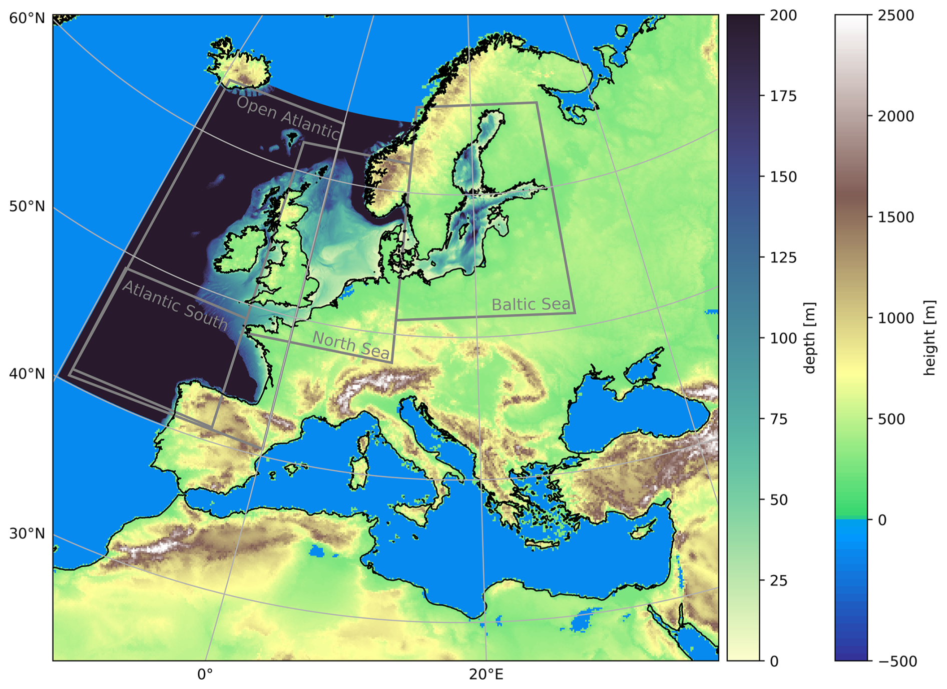
Figure 1 EURO-CORDEX domain (EUR-12) used for ICON-CLM (the corresponding colorbar is labeled with “height”) and NEMO-NBS bathymetry (colorbar labeled with “depth”). Grey quadrangles denote boxes used in the evaluation.

To make ICON more suitable for climate projections, the model had to be adapted for the use of the transient climatologies of aerosol and ozone. These adaptations were mainly done for the new global ICON-based Earth System Model, ICON-XPP (Müller et al., 2025a, b): For ozone, the CMIP6 dataset (Checa-Garcia, 2018) is used. The aerosol climatologies used originate from ECHAM6 (Stevens et al., 2013), namely the anthropogenic aerosol climatology MACv2 developed by Kinne et al. (2013) and Kinne (2019), but in the simple-plume version (MACv2-SP, Stevens et al., 2017), and an extended volcanic aerosol climatology based on Stenchikov et al. (1998). However, the Kinne aerosols provide different input parameters compared to the default aerosol climatology used in ICON for NWP. While different species are available from the aerosol climatology of Tegen et al. (1997) in the NWP version, which allows to infer properties like hygroscopicity, this distinction of different species is not available for the Kinne aerosols. In NWP, the aerosol properties are used to determine the influence of aerosols on cloud droplet numbers, which are an important quantity in cloud microphysics, with a secondary effect on radiation. Using the Kinne aerosols, the aerosol-cloud coupling was lost and had to be replaced with an alternative treatment. It was decided not to use the scaling factors available from the simple plume scheme (Fiedler et al., 2019), as these depend on assumptions, but to use a climatology of cloud droplet number concentrations (CDNCs) derived from satellite measurements. The non-transient, but monthly varying climatology used here is from Gryspeerdt et al. (2022) and was adjusted with a climatology of ECMWF (MODIS CDNC climatology based on Bennartz and Rausch, 2017; Grosvenor et al., 2018).

Another difference to the NWP setup is the use of a soil-type distribution of the Harmonized World Soil Database v2.0 provided by the Food and Agriculture Organization of the United Nations (FAO). As recently in NWP, the urban parameterization TERRA_URB was switched on (Zängl et al., 2025).

Note that the simulations and the raw output of ICON are done on an icosahedral, irregular grid (R13B5 in ICON notation). However, the raw output is interpolated using the nearest-neighbour approach onto the common EUR-12 grid (Fig. 1) and all evaluations for the atmospheric part are, therefore, also done on this rotated longitude-latitude grid.

For EURO-CORDEX, the evaluation simulation for ICON-CLM that will be published on ESGF was generated within the project “Updating the data basis for adaptation to climate change in Germany” (UDAG). Hereafter, this simulation will be called ICON-CLM-UDAG. The latest tuning for ICON-CLM was done in a joint effort of the UDAG project and the CLM community (an article on the tuning of ICON-CLM for CORDEX-CMIP6 is under preparation). For ICON-CLM as well as for ROAM-NBS, an important tuning target was the reduction of a positive surface shortwave radiation bias over land and ocean. In the current version, a tuning of the cloud cover scheme (monthly varying allow_overcast parameter) is applied. One setting that was not modified in ICON-CLM-UDAG compared to NWP, but in our ICON-CLM and ROAM-NBS simulations, was the minimum diffusion coefficient for heat tkhmin. It was increased from 0.6 to 0.8 for the winter months December through February. The effects of this modified setting will be discussed in Sect. 3.2.1.

For ROAM-NBS as well as for UDAG and ICON-CLM, the open source release icon-2024.07 was used. However, the OASIS3-MCT interfaces necessary for the NEMO coupling are not included in the official version as YAC is the only coupler supported by the ICON consortium. Therefore, the modifications of the feature branch containing the OASIS3-MCT interfaces are made available via github.

2.2 NEMO-NBS

The ocean component is based on the Geesthacht Coupled cOAstal model SysTem (GCOAST) setup, developed within the coastal model framework of HEREON (Staneva et al., 2016; Ho-Hagemann et al., 2020; Grayek et al., 2023). In the original GCOAST setup, NEMOv3.6 is used in the regional setup for the North West Shelf and the Baltic Sea (Staneva et al., 2016; Grayek et al., 2023). The main feature of the GCOAST setup is the enhanced representation of the coastal processes in the larger European shelf domain (Fig. 1), together with North and Baltic Seas, allowing a horizontal resolution of 2 nm and mixed σ–z^*-coordinates with 50 vertical layers. This vertical coordinate allows for the representation of the deeper and shallower regions simultaneously and consists of a predominantly σ-coordinate with a hyperbolic transient transition between the top and bottom layers following Madec and Imbard (1996). While creating the domain file containing the smoothed bathymetry used by NEMO, a slope is determined at which the terrain-following σ-coordinate intersects the sea bed and becomes a pseudo z-coordinate. This transition leads to a smaller bottom-level index in areas with steep slopes, like the North West Shelf. A high resolution in the upper layers (<0.18 m in the top layer and <1.0 m within the upper 16 layers) leads to a good representation of the ocean's interface to the atmosphere. The physical parameterizations and their settings were also chosen as in Ho-Hagemann et al. (2020). In the turbulence parameterization, the Generic Length Scale closure is chosen for vertical diffusion, and a geopotential Laplacian operator is used for the lateral diffusion of the tracers. The iso-level bilaplacian operator is applied within the momentum equations. The three-dimensional eddy-diffusivity is set to 0.01 m² s⁻¹ in the Atlantic and deeper layers, 0.01 m² s⁻¹ in the North Sea, and 0.3 m² s⁻¹ within the Baltic. A constant eddy-viscosity of 2.8×10⁸ m² s⁻¹ is applied throughout the simulations.

A number of changes were made to the original GCOAST version: In the current work, the updated NEMOv4.2.0 (Madec et al., 2022) with a new sea ice model SI3 (Vancoppenolle et al., 2023) instead of NEMOv3.6 was used. Besides the model version, an updated bathymetry from the European Marine Observation and Data Network (EMODnet) framework (EMODnet Bathymetry Consortium, 2020), which comes with a finer resolution, especially relevant for the coastal representation, has substituted the General Bathymetric Chart of the Oceans (GEBCO)-based bathymetry. Further, manual fine-tuning of the German coasts and Danish straits and a Laplacian smoothing were applied to the EMODnet data. In Fig. 1, the depths below 200 m are set to dark blue to accentuate the European North West Shelf area. Another modification to the original GCOAST setup was made in the radiation scheme: a three-band RGB radiation scheme instead of a two-band scheme was used. This scheme allows for a differentiated treatment of radiation in the North and Baltic Seas, enabling a better representation of highly stratified zones. The spatial variability in radiation is represented through a two-dimensional climatological field, which captures the mean chlorophyll concentration. This field serves as a prescribed parameter for the RGB radiation scheme. Since neither ROAM-NBS nor NEMO-NBS includes a biogeochemical module, the chlorophyll field is derived from literature and observational datasets: Schernewski et al. (2006) for the Baltic Sea, OSPAR Comission (2017) for the North Sea, and NASA Earth Observations (2024) for the Atlantic Ocean. Due to this change, a different radiative penetration of the sea surfaces of the shallower Baltic Sea and the deeper North Sea could be achieved. The state-of-the-art Thermodynamic Equation of Seawater (TEOS-10, https://www.teos-10.org, last access: 26 June 2025) is applied within NEMO-NBS for the calculation of state variables.

The river runoff dataset was provided by the German Bundesanstalt für Gewässerkunde and combines observational data in German national waters with model results of the WaterGAP hydrological model (Müller Schmied et al., 2021).

In the NEMO stand-alone setup, atmospheric forcing fields of the ERA5 reanalysis (Hersbach et al., 2020) in an hourly temporal resolution are used. These comprise wind velocities at 10 m height, air temperature and dew point temperature at 2 m height, mean sea level pressure, downward solar and thermal radiations. The surface turbulence and momentum fluxes are estimated using the ECMWF (2018) bulk formulation as implemented in the Aereobulk package (Brodeau et al., 2017). An additional influence is set by adding atmospheric pressure as an inverse barometer sea surface height to the ocean momentum equation.

The main tidal constituents M2, N2, 2N2, S2, K2, K1, O1, Q1, P1, and M4 for both NEMO-NBS as well as the coupled ROAM-NBS are provided at the lateral boundaries using the FES2014 dataset (Lyard et al., 2021).

Within NEMO-NBS and ROAM-NBS, only the ice thermodynamics of the SI3 sea ice model is applied, using five ice categories and two ice layers.

This setup represents one of the first implementations of NEMOv4.2.0 with SI3 in a fully coupled regional system for the European shelf, North and Baltic Sea, with direct applicability to coastal hazard and climate risk assessments.

2.3 Coupling via OASIS3-MCT

ICON and NEMO are coupled via the OASIS3-MCT_5.0 coupler (Craig et al., 2017; Valcke et al., 2021). The interfaces within the ICON code are based on the implementation described by Ho-Hagemann et al. (2024). On the NEMO side, the OASIS3-MCT interfaces are used as provided with NEMOv4.2.0. In our setup, we are using exclusively the approach of the flux coupling (Ho-Hagemann et al., 2024), which has the advantage over the bulk coupling that both the atmosphere and the ocean model see the same turbulent fluxes. Additionally, as ICON incorporates a tile approach, the flux coupling ensures the best possible local conservation of energy on non-common grids without using an exchange grid as, for example, Karsten et al. (2024); when variables are sent from the atmosphere at lower horizontal resolution to the ocean via OASIS3-MCT, tiled quantities are used. This approach is very similar to the one used in ICON-XPP (Müller et al., 2025b). These tiled quantities are representative for the ocean and sea ice fractions, respectively, in each atmospheric model grid cell, and are used by the ocean for the computations for open ocean and sea ice. The respective quantities are solar shortwave radiation, momentum flux, and the so-called non-solar radiation, which is the sum of sensible heat flux, latent heat flux, and long-wave radiation. As the ice fraction is sent from the ocean model to the atmospheric one via OASIS3-MCT, the ice fractions of both models are consistent. In the default NWP and ICON-CLM setup, the sea ice scheme calculates the heat transfer within the sea ice, dependent on the current ice depth and a standard bottom temperature. It cannot generate new sea ice, but the ice thickness can decrease and ice albedo and surface temperature are determined depending on the heat transfer as well as on snow lying on the ice. To make the thermal part more consistent with the NEMO/SI3, which has a more detailed treatment of thermodynamical processes within sea ice, the sea ice albedo, thickness and surface temperature are transferred from the ocean to the atmosphere in our setup. The ocean albedo over water is not sent, as this option is not available in the default coupling setup of NEMOv4.2.0. Only the one over ice is available for the coupling. Over the ocean, ICON uses a formulation by Taylor et al. (1996) for the direct albedo and the value of 0.06 for diffuse albedo as in ECMWF's IFS model. Additionally, an albedo increase by whitecap cover after Séférian et al. (2018) is considered.

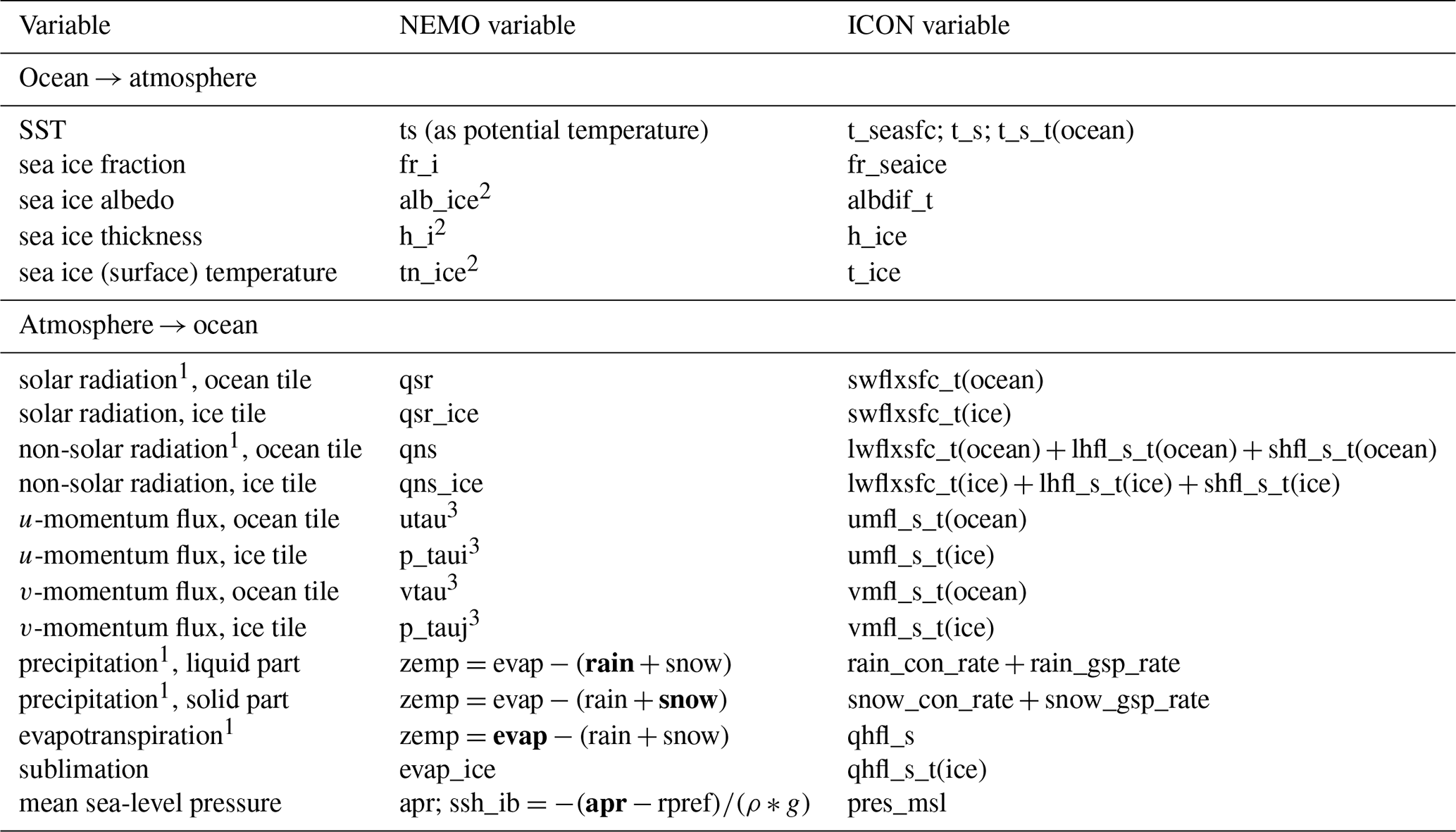
The complete list of variables exchanged during the coupling in ROAM-NBS is given in Table 1. For selected variables, a global conservation is applied, which means that the area average is compared before and after horizontal interpolation. By selecting “GLBPOS” in the OASIS3-MCT settings, the difference between the area average on the target minus the source grid is distributed proportionally to the value of the original field.

Table 1 Variables exchanged between the atmosphere and the ocean via OASIS3-MCT; for variables denoted by ¹, global conservation is applied by OASIS3-MCT after horizontal interpolation; NEMO variables denoted by ² are aggregated over all ice categories before sent to the atmosphere; NEMO variables denoted by ³ are rotated from the geographical to the local grid and staggered onto the U, V grid within NEMO; “ocean” or “ice” are given in parentheses for ICON variables to indicate that only the part of the variable on the respective tile is used. Variables that are combined into other quantities directly in NEMO's coupling interface are written in bold font.

Because only the respective portions of fluxes for the ocean and sea ice tiles are used, flux contributions from land points are completely excluded when fluxes are sent from the atmosphere to the ocean, which also ensures a consistent exchange of energy and momentum along the coastlines. As suggested by Mechoso et al. (2021) for models that incorporate the tile approach, the ocean fraction of the atmospheric model is adapted to that of the ocean model, which is obtained by interpolating the binary land-sea mask of the ocean model to the atmospheric grid. The land and lake fractions of the atmospheric model are adapted accordingly. For a correct treatment of coastal points, great care was put on identical interpolation methods for the NEMO land-sea mask and the NEMO fields to the ICON grid during coupling, as well as on the consistency of the common land-sea mask and the masks used by OASIS3-MCT. Thus, the flux coupling as included in ROAM-NBS is a good compromise between simplicity and correctness.

2.4 Overview of experiments and availability of reference data

The evaluation simulation was run for the coupled model (ROAM-NBS) and for both the atmospheric and ocean components individually (ICON-CLM and NEMO-NBS, respectively); i.e., we are overall evaluating and comparing three simulations. In Sect. 3.2.1, a basic comparison to the evaluation simulation from the UDAG project (called ICON-CLM-UDAG) is additionally shown. According to CORDEX specifications (CORDEX, 2025), “the evaluation experiment must cover at least the 1979–2020 period”. Our experiments were started in September 1978 because of the stable thermal mixed layer in the ocean. Starting in January would mean starting in the middle of the winter season when thermal conditions are unstable and the sea ice has already evolved, which has proven disadvantageous for model initialization, especially in coupled mode. To avoid a so-called “cold start”, a spin-up for the ocean component was carried out with NEMO-NBS for the years 1974–1978, starting with an initial field for temperature and salinity. This initial field was, in turn, a combined product from the ORAS5 reanalysis and the Baltic reanalysis product provided by SMHI (personal communication) based on Hordoir et al. (2019). The restart field for 1 September 1978 from the spin-up simulation with NEMO-NBS was then used to start ROAM-NBS.

For a better comparison of NEMO-NBS and the ocean part of ROAM-NBS, it was decided to use the same observation-based dataset for the runoff for both experiments. ICON-CLM as well as the atmospheric part of ROAM-NBS were started from the ERA5-driven ICON-CLM-UDAG simulation, which had been running since 1940.

For the atmospheric part, ERA5 reanalyses were used as lateral boundary conditions, as prescribed by the CORDEX-CMIP6 experiment protocol (CORDEX, 2025). They are available at a 3-hourly resolution and are also used to prescribe SST and sea ice in the uncoupled ICON-CLM simulation. For ROAM-NBS, ERA5 SST and sea ice fields are also used in ocean regions outside of the NEMO-NBS domain. As lateral boundary conditions for the ocean, the temperature, salinity, zonal and meridional ocean velocities, and sea surface height (SSH) fields from the ORAS5 global reanalysis dataset (Zuo et al., 2019) are used. The prescribed fields were used at a monthly resolution, as daily data were not available for the whole simulation period. To ensure that the spatial mean of the modeled SSH fits the observed SSH, the boundary conditions for the SSH from ORAS5 were bias corrected with respect to the SSH at Helgoland from the GESLAv3.0 observational data (Haigh et al., 2023). This bias was calculated on the basis of a 5-year test simulation with uncorrected boundary conditions.

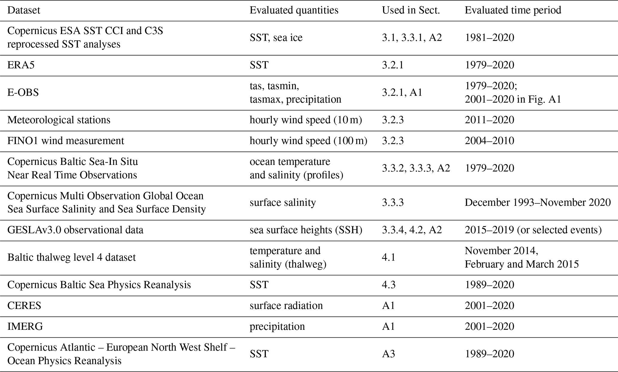
The evaluation is generally conducted for the years 1979–2020, which is the minimum period required for CORDEX. However, especially for the ocean part, many reference data are available for shorter time periods only, so that the evaluation period had to be adapted in these cases: SST and sea ice data (CMEMS, 2025a) are available from September 1981 and surface salinity from 1993 (CMEMS, 2023). Station data (CMEMS, 2024a) are very sparse before 1993. Copernicus reanalyses used for the evaluation of marine heat waves (CMEMS, 2024b, 2025b) start in 1989. For the atmospheric part, satellite data used for the evaluation of surface radiation (CERES; NASA/LARC/SD/ASDC, 2019) are available from 2001 only. Therefore, the evaluated time periods had to be adapted in these cases; an overview is given in Table 2. For evaluations in which statistics were calculated from hourly data, shorter time periods were used, partly due to limited data availability as well, partly to reduce the computational costs (see Sects. 3.2.3 and 3.3.4).

Table 2 Overview of datasets used for evaluation; references are given in the text; the full years were used if not denoted otherwise.

3 Evaluation of the mean climate

To assess the realism of the coupled ROAM-NBS system, we evaluate its representation of the present-day climate over the North and Baltic Seas in comparison with the atmosphere-only (ICON-CLM) and ocean-only (NEMO-NBS) simulations. The seasonal means are calculated for the main ocean-atmosphere surface variables to evaluate the performance of ROAM-NBS and its individual components with respect to climate timescales. Mean temperature and salinity profiles are validated in the Baltic to assess the ocean components' ability to model highly stratified regions. Statistical values for the sea surface height are presented for stations throughout the ocean domain.

3.1 Sea surface temperature

The most crucial variable at the interface of the atmosphere and the ocean is the SST, as it serves as the first indicator of the model's performance and proper coupling. Here, the simulated SST is compared to satellite observations from Copernicus. The Copernicus observations used are available from September 1981 to December 2024. Detailed information on the quality of the observational data is provided in the quality information document of the dataset, which can also be found on the product-specific Copernicus website. Figure 2a shows the difference between the simulated seasonal mean SST of ROAM-NBS and the observations. During winter (DJF) and spring (MAM), the area in the Northern Baltic is covered by sea ice with varying extent over time. In the Copernicus analyses, the SST is artificially set to −1.8 °C over the regions covered by sea ice. The points where these artificial SST values are found are masked out for the calculation of the mean differences.

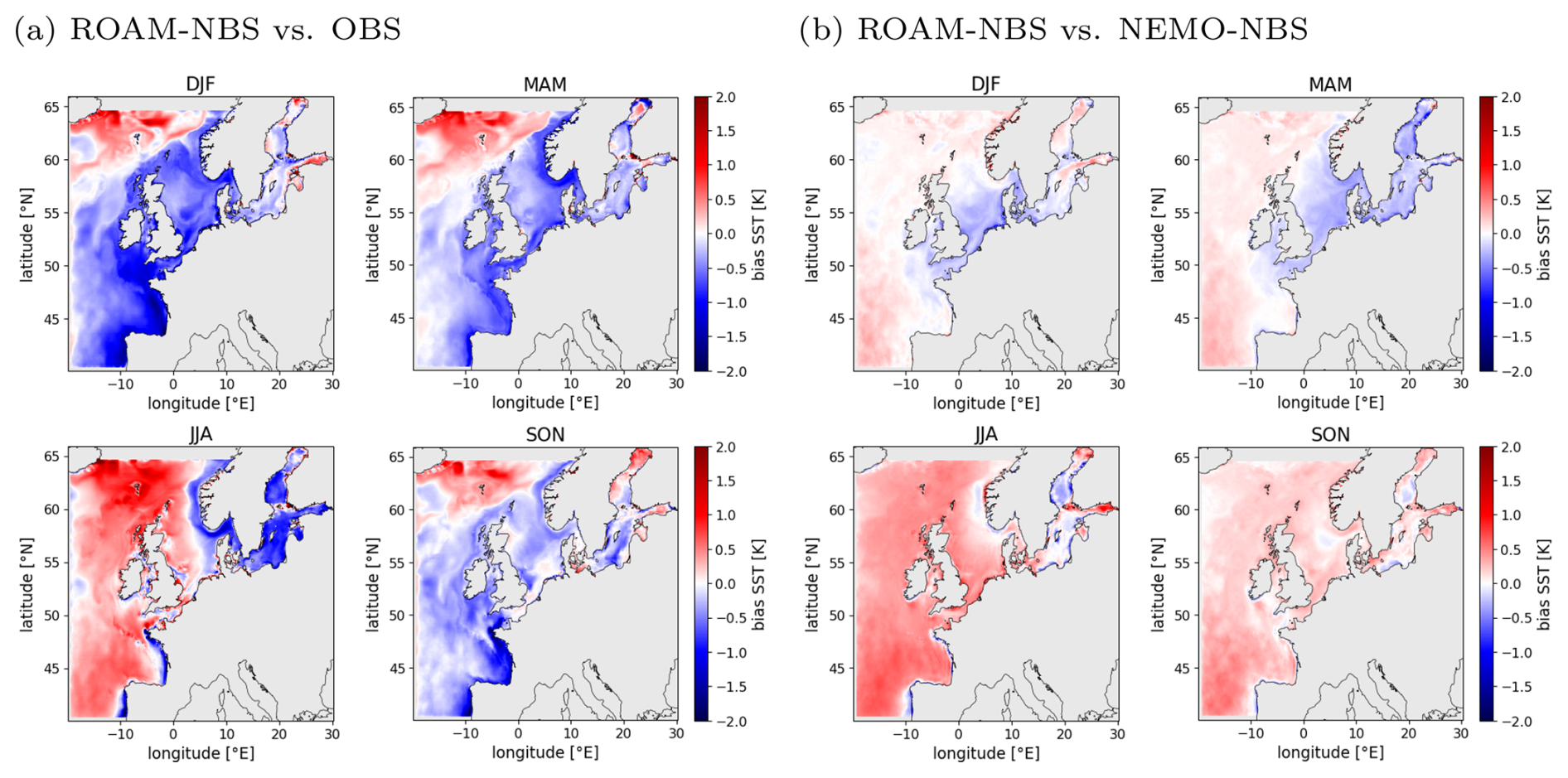
Figure 2 Seasonal mean sea surface temperature difference between ROAM-NBS and Copernicus observations (a) and ROAM-NBS and NEMO-NBS (b) for the period September 1981–November 2020.

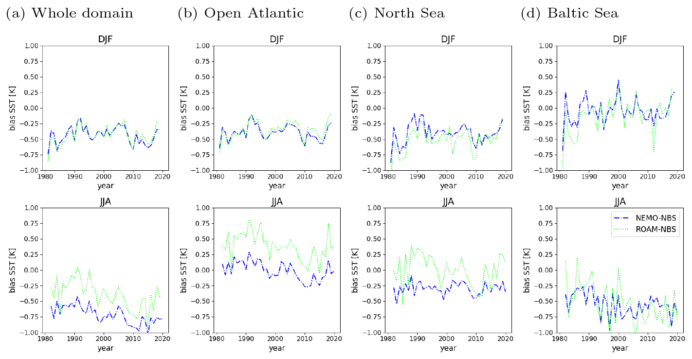
Figure 3 Bias of winter (DJF) and summer (JJA) seasonal mean SST time series for NEMO-NBS and ROAM-NBS to Copernicus observation data for the whole NEMO-NBS domain (a), Open Atlantic (b), the North Sea (c) and the Baltic Sea (d).

ROAM-NBS shows a cold bias of locally up to 2 K in the shallower regions of the European North West Shelf and in the Biscaya region during the colder seasons (SON, DJF, MAM). In the Baltic, the bias is around zero during these seasons. In summer, a positive bias can be observed in most parts of the NBS domain apart from the Baltic, where the bias becomes negative (up to −1 K in some years in the spatial average, Fig. 3d). A persistent warm bias is found near the northern Atlantic boundary, east of Iceland. This temperature bias could originate from the northward heat transport by the Gulf Stream at the surface and a too weak vertical diffusion/downward transport of heat at the model's boundary. The border between the positive and negative differences in all seasons except summer seems to envelope the European North West Shelf with a stronger bathymetry gradient, which could be a hint at an underestimation of Atlantic on-shelf transport (Ricker and Stanev, 2020) into the North Sea. In Fig. 2b, the difference between the seasonal mean SST of ROAM-NBS and NEMO-NBS is shown. The coupled simulation is generally slightly warmer than the uncoupled one, especially in summer (JJA). The tuning of the cloud cover scheme in ICON-CLM and ROAM-NBS reduced a positive surface shortwave radiation bias over land and ocean, so that it lies between ±10 W m⁻² (see Fig. A1) in the NBS region compared to CERES data. This reduction of the radiation bias contributed to a decrease in the positive SST bias in summer. However, it was not possible to reduce it further by a tuning of the atmospheric part. Eddy diffusivity in the eastern Atlantic was parameterized to be an order of magnitude higher than in the western Atlantic, which may have contributed to the cold bias observed near the French and Portuguese coasts.

Time series of the spatial mean seasonal SST biases against the Copernicus observations are shown for different regions in Fig. 3. The outlines of these regions (Baltic Sea, North Sea, Open Atlantic, and the whole domain) are shown in Fig. 1. As for the bias maps, points with ice cover in the observations were masked out for the calculation of the biases. For the whole domain, the area-averaged bias is about −0.5 K for both simulations in winter (DJF, Fig. 3a, upper panel). In summer (JJA, Fig. 3a, lower panel), the bias is slightly larger for NEMO-NBS (about −0.75 K), but smaller for ROAM-NBS. However, this smaller bias for ROAM-NBS in summer is due to the higher warm bias in the Atlantic (Fig. 3b, lower panel), combined with a negative bias in the Baltic Sea (Fig. 3d). The magnitudes of the biases for the Open Atlantic region and the North Sea are similar to those for the whole domain, or even smaller. In these regions during the summer season, ROAM-NBS is warmer than NEMO-NBS by about 0.3 to 0.4 K. In the Baltic Sea region, the SST biases in both simulations fluctuate around zero in winter while reaching −0.75 to −1 K during summer. As the spatial averaging of biases may cancel out positive and negative values, the time series of the RMSE are additionally shown in Fig. A4. Especially in the Baltic Sea, the RMSE is, with values of about 1.5 K in summer, higher than the absolute values of the mean bias. In the Open Atlantic and the North Sea, it is comparable to or slightly higher than the mean bias, with about 0.75 K in all seasons. The present SST biases in DJF and JJA (Fig. 3) as well as the RMSE (see Fig. A4) in all seasons and areas remain reasonably stable during the evolving simulation. Thus, no accumulation of errors takes place. The time series for the absolute area-averaged SSTs (see Fig. A4) demonstrate that the year-to-year variability as well as warming trends in the North and Baltic Sea are well reproduced in both simulations.

3.2 Meteorological conditions

3.2.1 Surface and near-surface temperatures

Over the ocean, the seasonal mean surface temperature differences between ROAM-NBS and ERA5 (Fig. 4a) mainly reflect the bias of NEMO against the Copernicus observations with too low SSTs in winter and too high SSTs in the Atlantic in summer. The differences between ROAM-NBS and ICON-CLM (Fig. 4b) over the ocean are identical to the ROAM-NBS/ERA5 differences by design, as ICON-CLM uses ERA5 SSTs as a lower boundary condition over the ocean. Over land, the differences are small (i.e. $<\pm \mathrm{0.25}$ K) compared to the biases against ERA5.

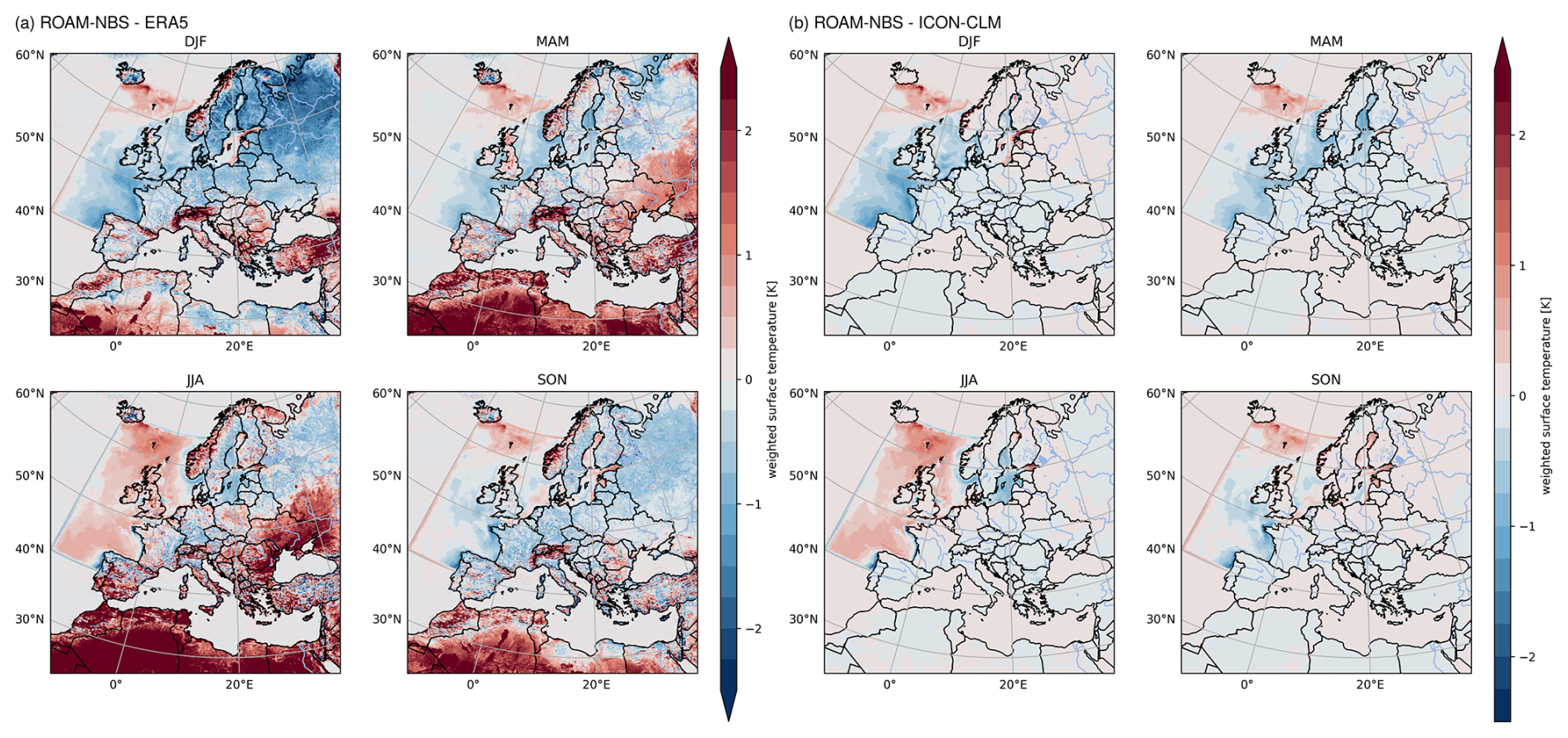
Figure 4 Mean seasonal surface temperature difference between ROAM-NBS and ERA5 (a) and ROAM-NBS and ICON-CLM (b) for the whole evaluation period (1979–2020).

As mentioned in Sect. 2.1, identical parameter settings as in ICON-CLM-UDAG were used in the ICON-CLM and ROAM-NBS simulations, apart from the increased minimum diffusion coefficient for heat. The higher minimum diffusion coefficient increases vertical mixing, especially in stable boundary layers, causing downward mixing of warmer air and an increase in near-surface temperatures. This adaptation was made to compensate for the wintertime SST cold bias of NEMO-NBS, which can also influence the air temperatures directly downstream of the ocean regions. However, from the evaluation of air temperature at 2 m (tas) against the E-OBS dataset (Cornes et al., 2018), which is available over land only, it is obvious that too low diurnal maximum temperatures (tasmax) are still prevailing (Figs. 5c and A2b) in ROAM-NBS. At the same time, minimum temperatures (tasmin) have a small warm bias compared to E-OBS (Figs. 5b and A2a). For the diurnal average tas, the ICON-CLM-UDAG simulation is up to 0.7 K too cool in winter for the entire E-OBS domain (Fig. 5a). The diurnal minimum (tasmin) in ICON-CLM-UDAG is too high in almost all regions and all months, with maximum biases of about 0.45 K in summer for the whole E-OBS domain average (Fig. 5b). At the same time, the diurnal maximum is up to 1.2 K too low in ICON-CLM-UDAG (Fig. 5c). Thus, the amplitude of the diurnal cycle is too low on average.

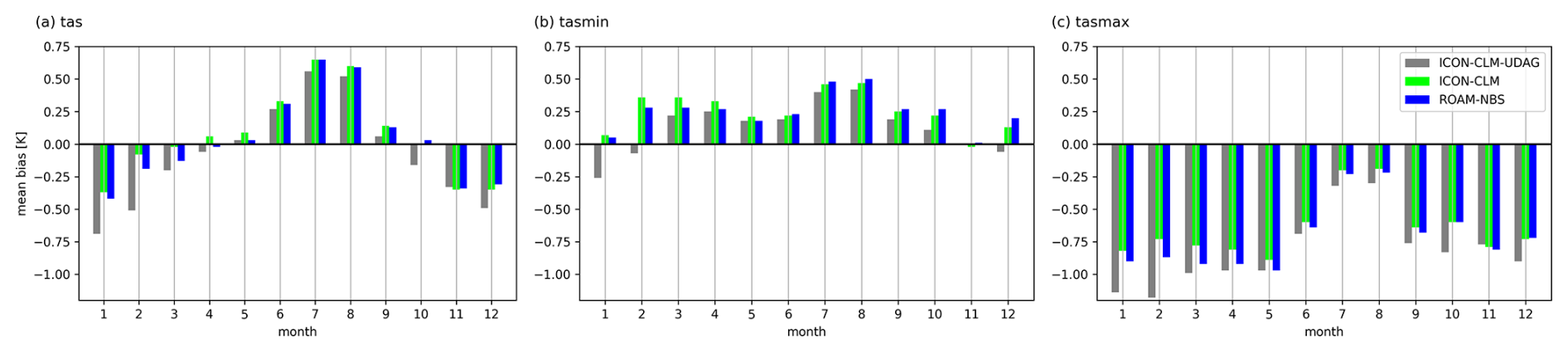
Figure 5 Monthly and spatial mean biases of tas, tasmin, and tasmax against E-OBS for ICON-CLM-UDAG, ICON-CLM, and ROAM-NBS, averaged over 1979–2020.

The increased minimum diffusion in ICON-CLM decreases the diurnal mean temperature bias in winter (DJF), while it is slightly increased from May to September. Accordingly, minimum and maximum temperatures are increased, which means that the already positive minimum temperature bias is getting larger. The largest positive minimum temperature bias of 0.8 K can be observed in February in Scandinavia.

To sum it up, the wintertime cold bias of ICON-CLM-UDAG is reduced by the adapted tuning parameter in ICON-CLM by about 0.2 K, at the cost of an increased warm bias of the diurnal minimum by about the same order of magnitude. However, the absolute values of the negative tasmax bias are still larger than those of the positive tasmin bias, apart from July and August.

Comparing ROAM-NBS and ICON-CLM, we can say that the positive diurnal mean and minimum bias are slightly higher in ROAM-NBS than in ICON-CLM, with a very similar bias for the diurnal maximum. As expected, the wintertime SST cold bias of the ocean is also slightly reflected in the temperatures over land.

3.2.2 Precipitation and flux differences

To give an overview of precipitation and fluxes over the ocean, for which good measurement products are not available or are not at a sufficient spatial resolution to adequately evaluate the NBS region, the differences between the coupled and uncoupled simulations are analyzed here. For completeness, seasonal mean bias maps are provided for precipitation and surface net longwave radiation in Fig. A1 in the Appendix. As the SST is prescribed for ICON-CLM, the SST differences between ROAM-NBS and ICON-CLM also reflect the bias against observations, which does not directly mean that the precipitation and flux differences between both simulations, as shown here, reflect biases. However, they can give a good indication of the reaction of the coupled model to SST biases.

For precipitation, the differences between ROAM-NBS and ICON-CLM reflect the differences in evaporation or latent heat flux (hfls) over the ocean (Fig. 6): Precipitation over the ocean is higher by up to 0.15 mm d⁻¹ in ROAM-NBS in regions where evaporation is higher, such as over the Atlantic ocean and North Sea in summer or the Baltic Sea in winter. Vice versa, precipitation is lower by up to −0.15 mm d⁻¹ when evaporation is lower, as over the Atlantic ocean and the North Sea in summer. However, these differences are small compared to the absolute precipitation biases over land, which exceed ±0.6 mm d⁻¹ in various regions (Fig. A1b and d; note the adapted color scale compared to Fig. 6).

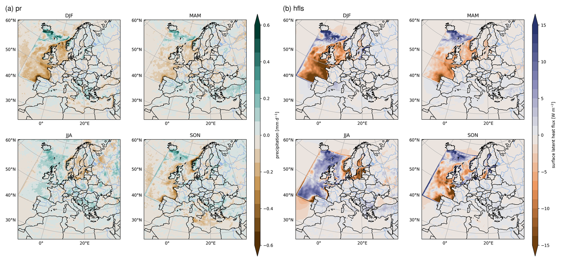
Figure 6 Seasonal mean difference of precipitation (pr, a) and latent heat flux (hfls, b) of ROAM-NBS against ICON-CLM, averaged over 1979-2020.

The mean values of precipitation and evaporation differences between ROAM-NBS and ICON-CLM are also provided for different ocean domains in Fig. 7, together with the differences for sensible heat flux (hfss), 10 m wind speed (sfcWind) and surface temperature (Tsfc). Tsfc over the (ice-free) ocean in ICON is equivalent to the SST. The absolute differences clearly show that the sign of the Tsfc difference determines the sign of the flux, sfcWind and pr differences. For example, for a lower Tsfc of ROAM-NBS as in the Open Atlantic, Atlantic South and North Sea boxes in DJF and the Baltic Sea box in JJA, also hfls, hfss, sfcWind, and pr are lower than in ICON-CLM. Accordingly, all differences in the Open Atlantic, Atlantic South and North Sea boxes in JJA are positive. The only exception is the Baltic Sea in DJF, where the spatially averaged Tsfc differences are very small (below −0.05 K). The absolute area-averages for ICON-CLM (given as numbers in Fig. 7) show that the fluxes, and therefore, also the flux differences become higher over a warmer ocean surface. Looking at the Atlantic South and the North Sea in DJF, for example, the Tsfc difference is very similar in both regions (−0.45 and −0.43 K, respectively), but the heat flux difference is larger for the Atlantic South (−10.57 W m⁻² for the sum of hfls and hfss compared to −9.13 W m⁻² for the North Sea). But the Atlantic South is, on average, warmer than the North Sea (286.1 K compared to 280.8 K). However, the absolute temperatures of the ocean surface cannot explain all differences; otherwise the fluxes would be much higher in JJA than in DJF. The temperature and humidity of the overlying air masses, as well as the mean wind speed, also have an influence. The sfcWind differences are shown as their interpretation is more straightforward than that of the momentum flux, which is given as u and v components. The sign of the sfcWind differences being in agreement with the flux differences shows that more mixing due to higher surface temperatures does not only result in stronger turbulent heat fluxes but also in more downward mixing of horizontal momentum and, thus, in higher near-surface wind speeds (and vice versa). In conclusion, SST biases, which are already present in NEMO-NBS and introduced into the coupled simulation, are directly reflected by the turbulent heat fluxes, near-surface wind speed and precipitation. However, these biases have no systematic impact on the land areas.

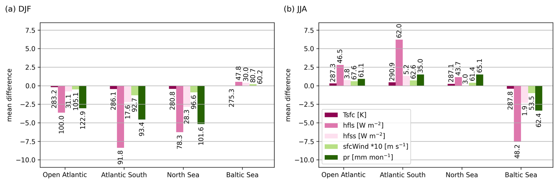
Figure 7 Mean absolute differences of ROAM-NBS against ICON-CLM for winter (a) and summer (b) for different quantities (see legend), averaged over four different regions, excluding the land parts, and over 1979–2020. The numbers indicate the mean values of ICON-CLM for the respective quantities.

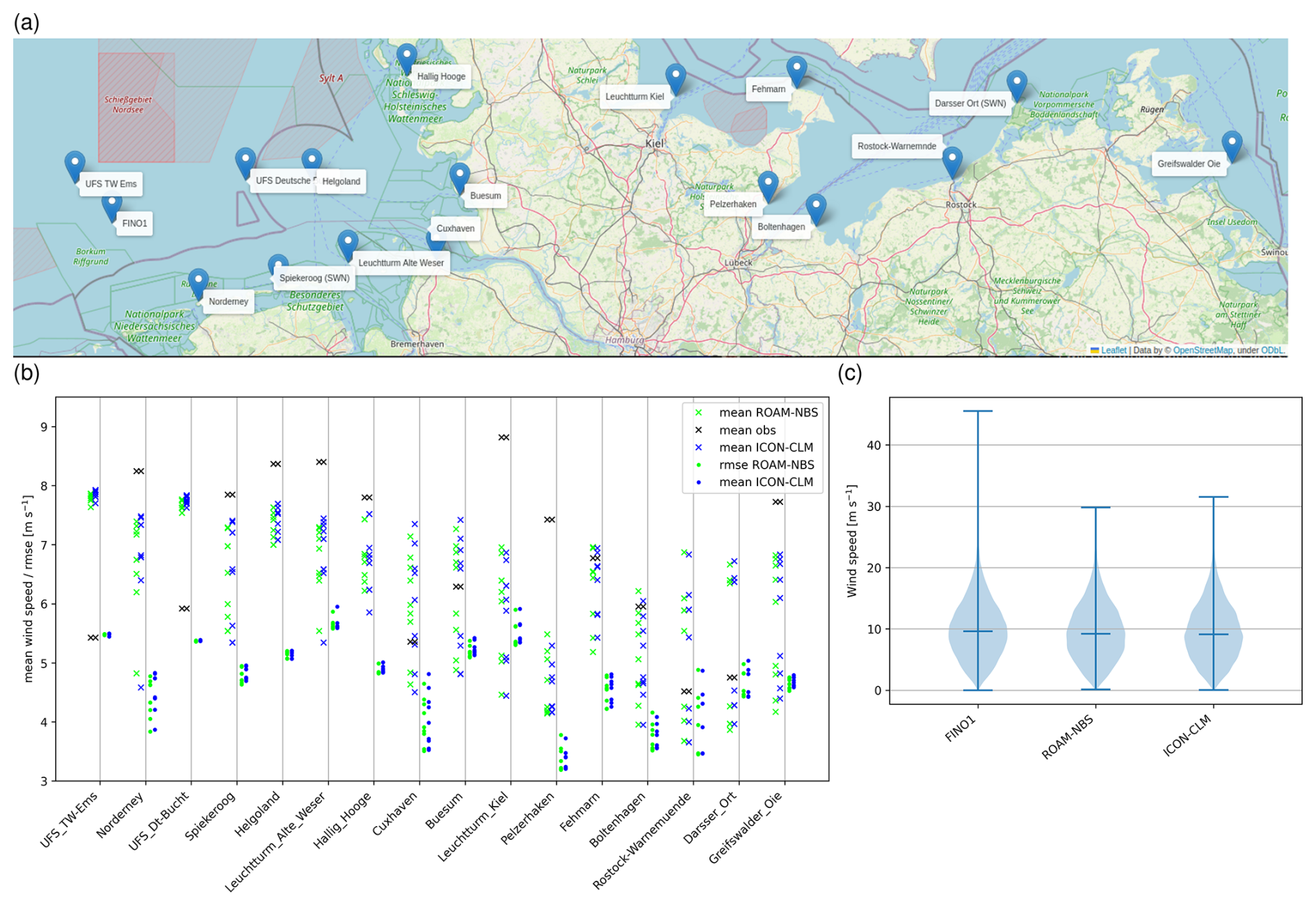
Figure 8 Map with an overview of the evaluated station observations (a); mean station observations of hourly wind speed for 2011–2020, mean values and root-mean squared errors (rmse) of 9 closest grid points for each station for ROAM-NBS and ICON-CLM (b); violinplot displaying median, minimum and maximum values of hourly wind data at 100 m height at FINO1 and at the closest grid points in ROAM-NBS and ICON-CLM, for the years 2004–2010 (c).

3.2.3 Wind speed

For a more detailed evaluation of simulated wind speed, DWD station observations along the German coast as well as the wind measurements at 100 m height at the FINO1 platform were used. The locations of the stations as well as of FINO1 are indicated in Fig. 8a. The surface station evaluation was done for hourly wind speed for the years 2011–2020, which was the period with the most common observations. FINO1 was evaluated only up to 2010, as the wake effect of the wind farms at this location is too large after 2010 (e.g. Spangehl et al., 2023). For the surface stations, the nine closest grid points were used to capture the variability due to a potential mismatch between the coastline in the model and in the real world as well as unresolved geographical features. For FINO1, however, only the closest grid point was selected as the platform is located in the North Sea about 45 km away from the German coast and the measurement is taken at 100 m height, where surface effects have less influence. For both the surface station as well as the FINO1 comparison (Fig. 8b and c), an underestimation of wind speed over the ocean by both ROAM-NBS and ICON-CLM can be seen. The violinplot for FINO1 illustrates that both the mean and the maximum wind speed are underestimated, as both the median and the maxima are smaller in the simulations. The underestimation seems to be strongest for stations further away from the mainland like those on lighthouses and floating devices (“UFS Deutsche Bucht”, “Leuchtturm Kiel”, “UFS TW-Ems”, “Leuchtturm Alte Weser”). For most of these, the spatial variability is small (indicated by the dots lying closer together in Fig. 8b). However, at least the wind measurements on lighthouses are not taken at a height of 10 m but further up at about 40 m, which explains the strong underestimation displayed in Fig. 8b. In most cases, ICON-CLM displays a slightly higher wind speed than ROAM-NBS, but this is not surprising as the SST bias in ROAM-NBS along the German Coast is on average slightly negative, which also causes a negative wind speed bias.

The underestimation of wind speed is weaker, but still discernible for stations on smaller islands like Helgoland, Büsum, Spiekeroog or Hallig Hooge. An exception is Norderney, but here it is unclear why the mean observed wind speed is by about 2 m s⁻¹ smaller than at Spiekeroog, which is relatively close. In contrast, for most stations on the coast or for Fehmarn, which is a larger island compared to those in the North Sea, the mean wind speed is well represented by both ROAM-NBS and ICON-CLM, and the RMSE values are also small compared to other stations.

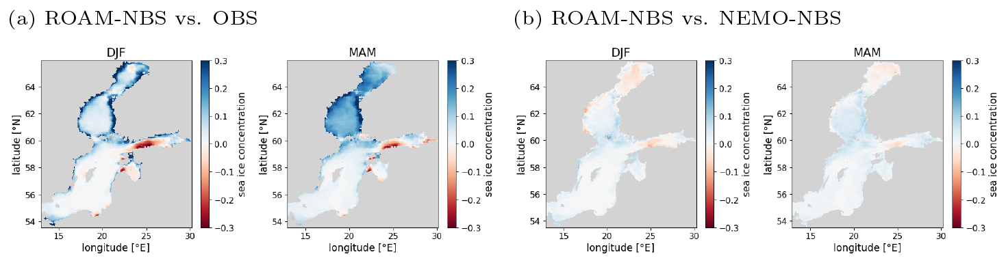
Figure 9 Differences in the mean sea ice concentration for ROAM-NBS vs. Copernicus observations (a) and ROAM-NBS vs. NEMO-NBS (b) for winter and spring for September 1981–November 2020.

3.3 Oceanographic conditions

3.3.1 Sea ice concentration and extent

The bias of ROAM-NBS and NEMO-NBS against the Copernicus observations for the winter season (DJF) is small (Fig. 9a), and the difference between ROAM-NBS and NEMO-NBS is negligible (Fig. 9b). Nevertheless, in the spring season (MAM), the amplification of sea ice extent is prominent in the Gulf of Bothnia. While the start of the ice growth season and the growth rate in the end of December are well captured, the sea ice extent is overestimated during the peak later in winter (February-March) by both simulations (mean annual time series of sea ice extent not shown). Furthermore, the sea ice season is prolonged towards May compared to the observations. The overestimation of sea ice concentration as well as extent in MAM might originate from the prevailing negative bias in SST in the Bothnian Bay and Sea during winter and spring (Fig. 2 and the temperature profile for DJF at SMHISR5C4 station in Fig. 10) and an underestimation of salinity, especially in the Gulf of Bothnia (see the next subsection). Further, in Nie et al. (2023), the NEMO-SI3 model for version 4.0 was found to be most sensitive to the ice–ocean and atmosphere–ice drag coefficients and, therefore, to ice dynamics. Since only thermodynamical processes are modeled within ROAM-NBS and NEMO-NBS, further enhancements in results could be obtained by also considering ice dynamics. First tests with ice dynamics did not improve the overestimation of sea ice in spring. They will need to be carried out in the future in combination with further parameter tuning and recalibration to eliminate the temperature and salinity bias in the Northern Baltic.

3.3.2 Ocean temperature

In addition to the SST evaluation in Sect. 3.1, the evolution of temperature in different depths over time and mean temperature profiles are compared against observational profiles for the ROAM-NBS and NEMO-NBS simulations to evaluate the stratification of the Baltic. The chosen stations, resembling those of Meier (2007), cover the main basins of the Baltic Sea and are displayed in Fig. 10a. The observational data are in-situ profile data from Copernicus. The seasonal mean is calculated over all time instances between January 1979 and December 2020 where the observational data exist.

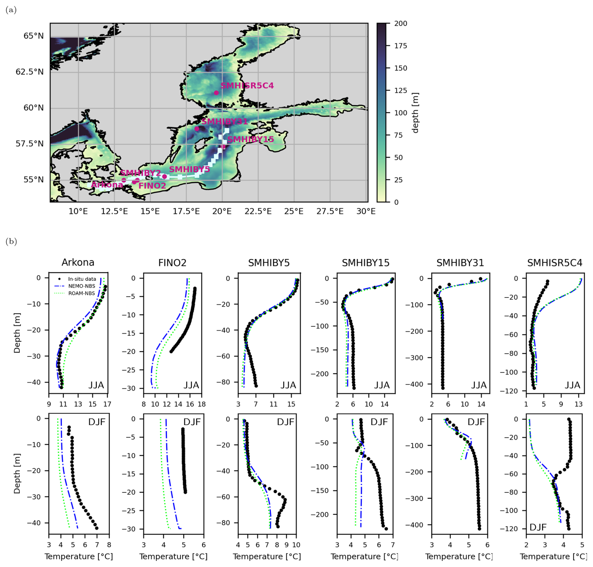
Figure 10 Baltic section of applied bathymetry in NEMO-NBS and ROAM-NBS. The stations used for the temperature and salinity mean profile validation as well as time series (magenta) and the IOW Baltic thalweg measurement path on 11 November 2014 (lightblue) as given in Mohrholz (2016) are displayed (a); seasonal mean temperature profiles (January 1979–December 2020) at Baltic stations (b).

At the monitoring stations Bornholm Deep (SMHIBY5) and Gotland Deep (SMHIBY15), both simulations tend to fit in-situ observations in the upper layers and underestimate temperatures in the deeper layers over the entire evaluation period (see Fig. A5). The seasonal cycle is captured by both simulations.

The mean temperature profiles in the Arkona Basin (Arkona and FINO2, Fig. 10b) generally match the observational data for both simulations. In winter, a cold bias of 1–2 °C can be quantified in the Arkona Basin, which is slightly stronger for ROAM-NBS than for NEMO-NBS. At FINO2, the mean profile for summer also reveals a cold bias of about 1.0 °C, here with NEMO-NBS being cooler than ROAM-NBS. At station SMHIBY5, which is located in the Bornholm basin, both model runs coincide well with observational data at the sea surface and in layers above a depth of 50 m; differences between the coupled and uncoupled simulations are small (Fig. 10b). In the bottom layer, a cold bias can be observed. This cold bias at station SMHIBY5 is larger in summer than in winter, whereas the intermediate layer is accurately captured in summer. Similarly, within the Gotland Deep (SMHIBY15, Fig. 10), both model runs underestimate the mean temperature at depths below 100 m, mostly due to a weak salinity stratification (see Fig. 12). The overall cold bias at the bottom of the Gotland Deep will also be shown in Sect. 4.1. As in the Arkona Basin, the coupled model ROAM-NBS has a larger cold bias in winter than the NEMO-NBS stand-alone run. The intermediate layer is well captured at station SMHIBY15 during the summer months.

The last two stations, SMHIBY31 and SMHISR5C4, lie in the Landsort Deep and Gulf of Bothnia, respectively. The shallow depth of the Landsort Deep in the simulations arises from Laplacian smoothing of the EMODNET bathymetry and the use of the nearest grid cell for station SMHIBY31, so that the deepest smoothed cell (370 m) does not align with the station's grid point. For the available model depth, both simulations' seasonal mean temperature results agree well with the observational data. In the Gulf of Bothnia in summer, both simulations exhibit a warm bias near the surface, but a small bias below 40 m. In winter, the sign of the surface and near-surface bias is reversed compared to summer. However, for the calculation of mean profiles, the model and observational datasets were not masked for ice concentrations, which contributes to larger discrepancies in surface and near-surface temperatures at station SMHISR5C4 during the winter months.

Overall, both simulations exhibit smaller temperature biases in summer than in winter. At most stations, the simulated temperatures align more closely with observations near the surface than in the deeper layers for both seasons. In summer, the temperature profiles also display an intermediate layer, although its magnitude is underestimated in both model runs.

3.3.3 Salinity

The model sea surface salinity is validated against an interpolated level-4 analysis of the sea surface salinity based on in-situ and satellite observations from Copernicus. The winter and summer differences between the simulated mean sea surface salinity of ROAM-NBS and observations for the period December 1993–November 2020 are shown in Fig. 11. These years were chosen as the observational dataset is only available for this period (Table 2). The sea surface salinity tends to be underestimated at the Norwegian and German coasts and the Baltic Sea and tends to be overestimated at the passage from the Baltic Sea to the North Sea. However, both models, ROAM-NBS and NEMO-NBS, show very similar results (Fig. 11). Since the pattern at the coasts seems to be quite constant throughout the year, the cause may originate from a prescribed inflow of fresh water that is too strong. Within the current NEMO-NBS and ROAM-NBS simulations, the runoff is prescribed only in the upper layer. A prescription over the complete water column and additional vertical mixing could better distribute the fresh water from the rivers and further enhance the sea surface salinity results. The underestimation of the salinity in the Baltic Basin may be the result of the general underestimation of the salinity inflow from the North Sea.

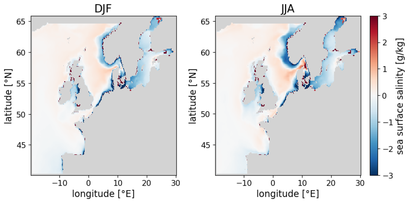
Figure 11 Seasonal mean (DJF and JJA) sea surface salinity difference between ROAM-NBS and observations for the period December 1993–November 2020.

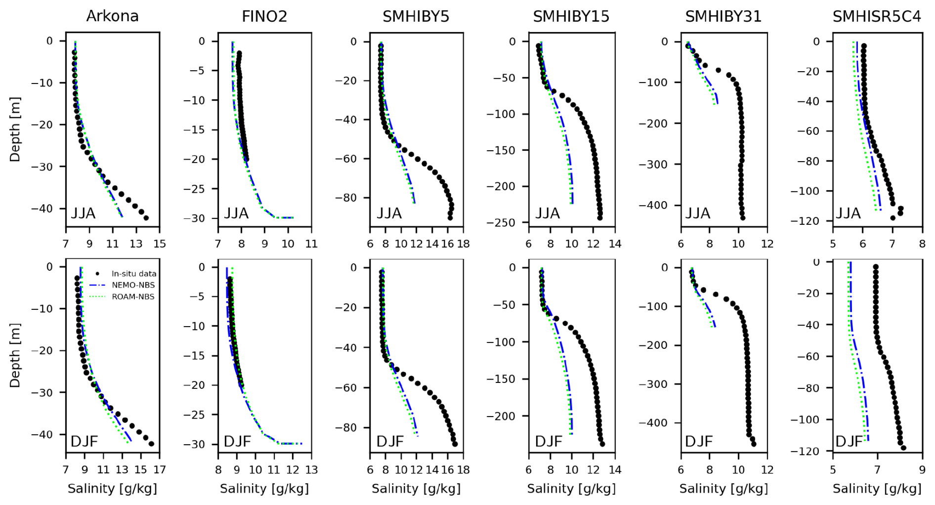
Figure 12 Summer and winter seasonal mean salinity profiles at Baltic stations for the period January 1979–December 2020.

Time series of surface and bottom salinity at stations SMHIBY2, SMHIBY5, and SMHIBY15 are shown in Fig. A6, illustrating the temporal variability at each site. Both models underestimate the salinity in deeper layers but fit observations in upper layers. The surface salinity biases derived from the time series (Fig. A6) range between 0.17 and 0.37 psu for NEMO-NBS, and between 0.05 and 0.41 psu for ROAM-NBS. At the bottom, the biases are more pronounced, spanning from −1.55 psu at SMHIBY2 to −4.38 psu at SMHIBY15 for NEMO-NBS, and from −1.87 psu at SMHIBY2 to −4.64 psu at SMHIBY15 for ROAM-NBS. The representation of the stratification of the Baltic Sea is further analyzed with seasonal mean profiles (Fig. 12) as well as sections through the Baltic in Sect. 4.1. Stratification is underestimated at stations SMHIBY5, SMHIBY15, and SMHIBY31 (Fig. 12). Enhancing its representation is essential for reliable coupling with biogeochemical models and for achieving accurate results. As an example, one Major Baltic inflow (MBI) event (2014) is chosen for the comparison between observations and simulations. The MBI is reproduced but underestimated at both stations.

The mean salinity profiles between 1979 and 2020 indicate an underestimation of salinity in the deep areas of both simulations (SMHIBY15, SMHIBY5, SMHIBY31, Fig. 12). The surface salinity is well represented at these locations by both ROAM-NBS and NEMO-NBS. This behavior is consistent throughout all seasons. At Arkona and FINO2 (Fig. 12), model results highly coincide with the mean observational salinity profiles. At FINO2, model results align well with observations in winter and autumn, while a minor fresh bias near the surface is observed during summer. In the Gulf of Bothnia (SMHISR5C4), both simulations show a fresh bias, which is slightly smaller for the NEMO-NBS stand-alone run than for ROAM-NBS. Seasonal profiles indicate that the fresh bias in the Gulf of Bothnia is mainly driven by the winter months. The discrepancy may result from the fact that neither observational nor model data were masked to account for existing ice during this period. Overall, an underestimation of bottom salinity in deeper Baltic basins can be observed. This underestimation could be mitigated in future simulations by employing longer spin-up periods or improved initial conditions. Additionally, efforts should focus on refining vertical and horizontal mixing within the Baltic and increasing spatial resolution in the Danish Straits. For climate projections based on the current setup, bias correction of bottom salinity values in basins deeper than 40 m is necessary.

3.3.4 Sea surface heights

To assess the accuracy of sea surface heights, model results are compared against GESLAv3.0 observational data within the evaluation period of January 2015 to December 2019. A period was selected during which all observational stations provided continuous hourly data, ensuring that the resulting statistics are fully comparable.

Here, the sea surface height results are bias adjusted by subtracting the mean of SSH within the evaluation period from SSH results. The storm surge component of the water level is assessed by removing the influence of astronomical tides from the bias-adjusted sea surface height. This is achieved using a Demerliac filter, which separates tidal fluctuations from the total signal. The remaining residual captures the non-tidal water level variations caused by meteorological forcing, providing an estimate of the storm surge. Scatter plots for the detided sea surface height (representing the storm surge) are displayed in Fig. 13 for a station in the German Bight (Cuxhaven, see Fig. 8), and the Baltic (Landsortnorra). Statistical values such as the number of data points N, the correlation coefficient r, the root mean square deviation rmsd, and the explained variance η are calculated and summarized in Table 3 for the detided sea surface heights (representing storm surge) at further stations covering the model domain.

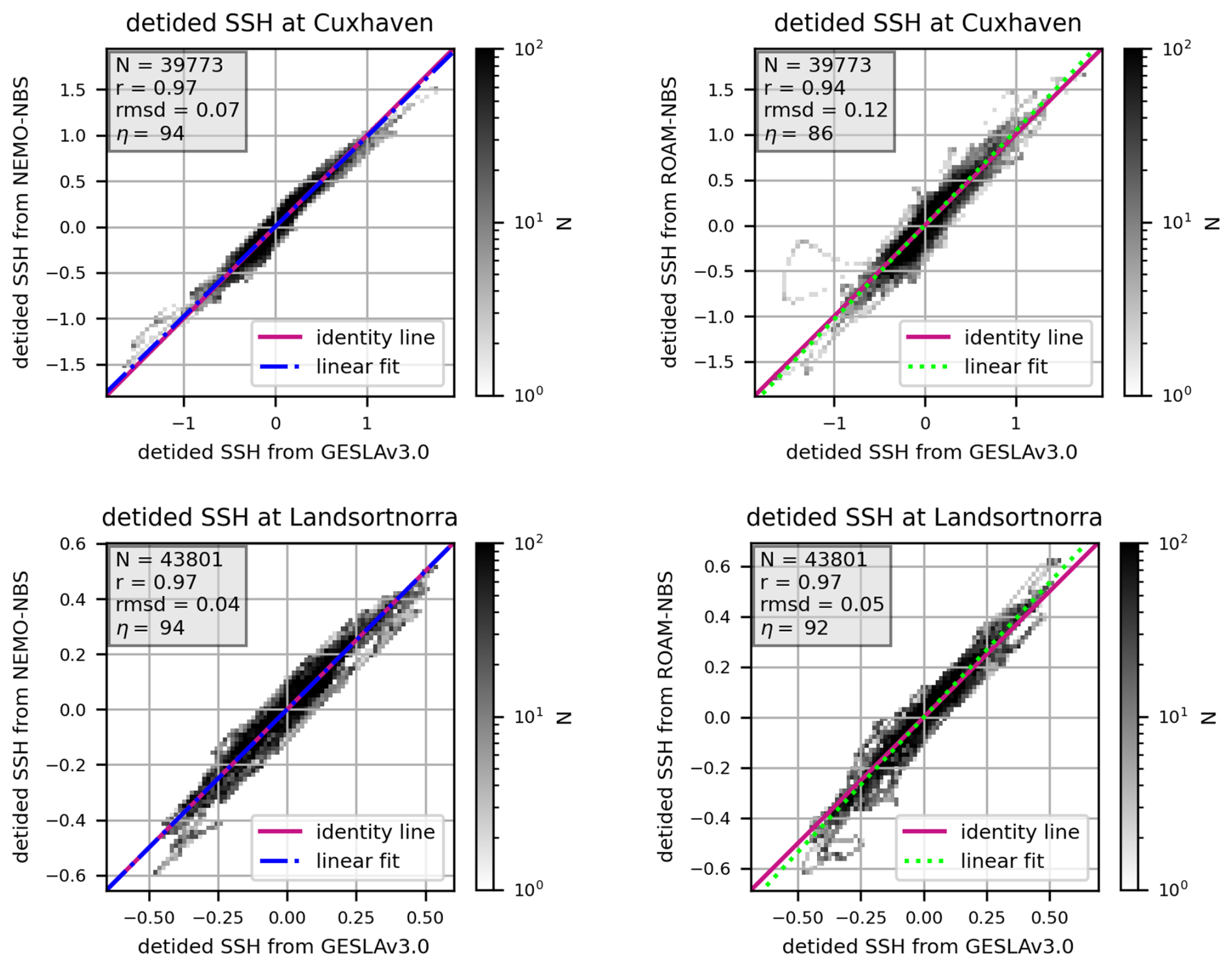
Figure 13 Comparison of scatter plots of detided sea surface heights at selected stations in the North Sea and Baltic for NEMO-NBS (left panels) vs. ROAM-NBS (right panels).

Table 3 Statistical values of detided sea surface height model results vs. GESLAv3.0 observational data evaluated within January 2015–December 2019.

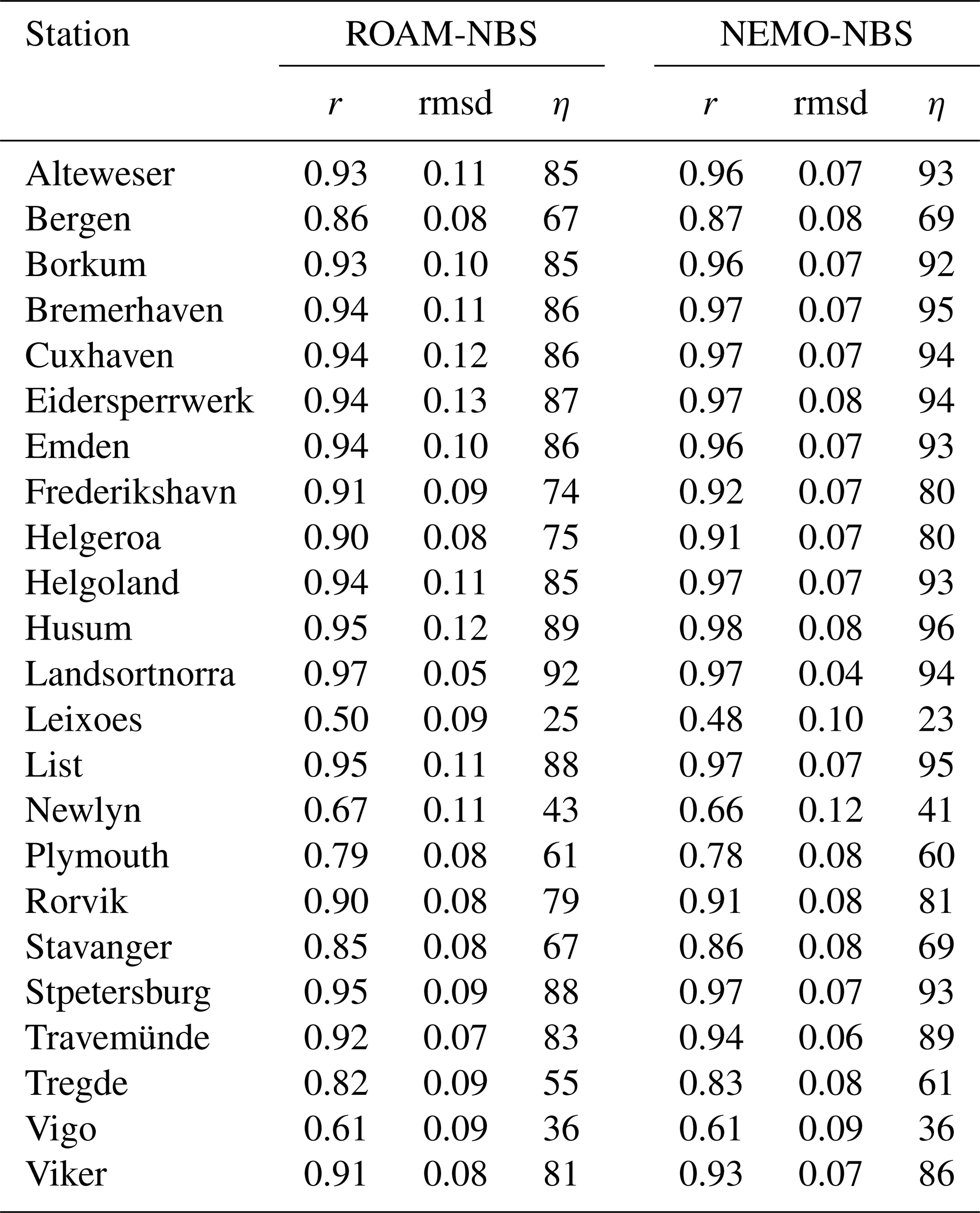
For detided sea surface heights, NEMO-NBS shows a higher correlation with the observational data than ROAM-NBS at nearly all stations, with minimal differences in correlation coefficients. The root mean square deviation of NEMO-NBS is smaller for the majority of the stations. As can be observed in the scatter plots, for detided sea surface height extreme values, especially maxima, ROAM-NBS performs better than NEMO-NBS in the German Bight, while it slightly overestimates maxima at Landsortnorra. The higher maxima at all stations obtained with the coupled ROAM-NBS simulation indicate a positive effect of the atmosphere–ocean coupling on wind speed quality. NEMO-NBS's performance for sea surface height maxima could be improved by calibrating the wind drag coefficient. Single storm events, which cannot be well represented spatially or temporally, lead to single outliers in the coupled model. These outliers are not present in the reanalysis driven NEMO-NBS results. Overall, the correlation of storm surge of both simulations with observational data is high, especially in German national waters. At stations closer to the domain boundaries, storm surge correlations could be improved. Nevertheless, overall bias-adjusted sea surface height results strongly correlate with observational data (see Fig. A7) for the coupled and uncoupled models due to a high tidal component.

4 Variability and extreme events

In this section, the model results of ROAM-NBS and NEMO-NBS are evaluated for exemplary extreme events against observational and reanalysis data. As an adequate representation of the inflow from the North Sea into the Baltic Sea is important for correctly modeling the state of the Baltic Sea over longer timescales, a particular focus was placed on the analysis of this inflow. In Sect. 4.1 and 4.2, cross-sections of salinity and temperature through the Baltic and sea surface heights at representative stations are evaluated around the Major Baltic Inflow (MBI) in December 2014, which was the third-largest recorded inflow. Its influences are described in Mohrholz et al. (2015). In Sect. 4.3, the model simulation's capacity to track observed marine heatwaves (MHWs) is examined.

4.1 Stratification along the Baltic Thalweg for the Major Baltic Inflow in 2014

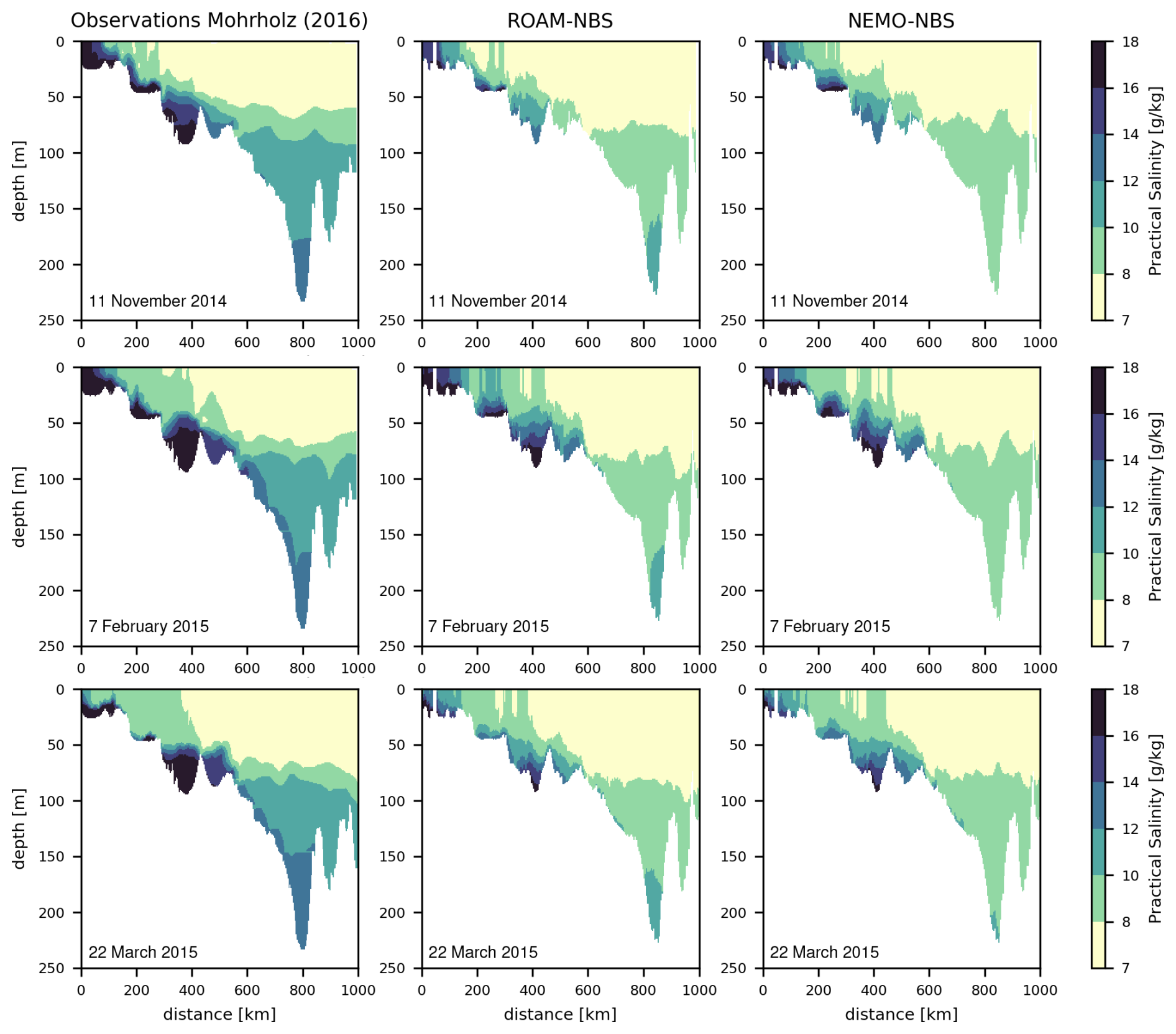
The Baltic Sea is characterized by its strong stratification of temperature as well as salinity, and its correct representation is needed for marine climate applications. To validate the stratification, the Baltic thalweg level 4 dataset (Mohrholz, 2016) is used for temperature and salinity. The interpolated gridded CTD (Conductivity, Temperature, Depth) dataset contains the longitudes and latitudes of the stations where measurements were taken, and these slightly vary with each observation cruise. Therefore, the exact coordinates of the bathymetry profiles along the Baltic thalweg in Figs. 14 and 15 may differ from date to date, but the model data is always extracted at the locations given in the observational data. An exemplary observational route is shown in Fig. 10a, and the distance along the route to the start is plotted on the x axis.

Figure 14 Conservative temperature along the Baltic thalweg for NEMO-NBS, ROAM-NBS and observational data (Mohrholz, 2016) at three time instances around the MBI 2014: 11 November 2014 (top panels), 7 February 2015 (middle panels) and 22 March 2015 (bottom panels).

Figure 15 Practical salinity along the Baltic thalweg for NEMO-NBS, ROAM-NBS and observational data (Mohrholz, 2016) at three time instances around the MBI 2014: 11 November 2014 (top panels), 7 February 2015 (middle panels) and 22 March 2015 (bottom panels).

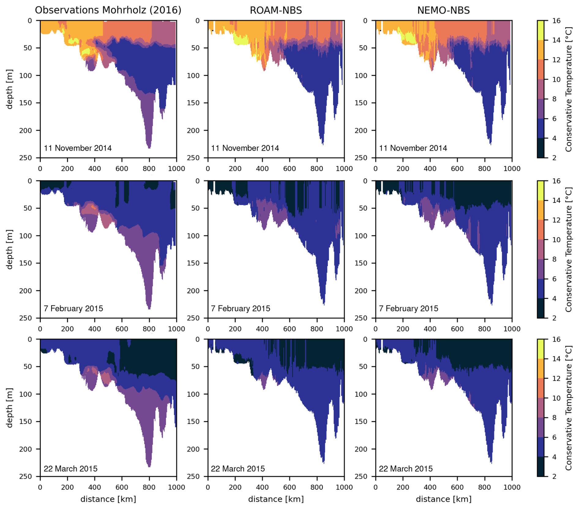
Under typical conditions, the inflow from the North Sea into the Baltic Sea through the Danish Straits is relatively moderate and exhibits a seasonal cycle. Inflow generally occurs as dense, saline water entering the Baltic and is strongest during late winter and early spring due to wind-driven and barotropic forcing (Matthäus and Franck, 1992; Mohrholz, 2018). These inflows gradually ventilate the deep basins of the Baltic and maintain the salinity balance (Lehmann et al., 2022). Under normal circumstances, the inflow is steady and predictable, with variations primarily controlled by seasonal winds, sea-level differences between the North Sea and the Baltic Sea, and long-term atmospheric pressure patterns (Mohrholz, 2018). Significant episodic events in which dense, saline water from the North Sea flows through the Danish Straits into the Baltic Sea, ventilating its deep basins and temporarily raising deep-water salinity and oxygen levels are called MBI events.

To evaluate the model simulation's capability to depict the inflow of saline water into the Baltic, thalweg profiles before the MBI 2014 (November 2014) and after the MBI event (February and March 2015) are displayed for temperature (Fig. 14) and salinity (Fig. 15).

As can be observed in Fig. 14, the temperature thalweg of the coupled ROAM-NBS and ocean stand-alone NEMO-NBS simulation only subtly differs. Before the MBI event, a temperature bias in the deep basins already existed between both model simulations and the observational data. The surface temperature obtained with NEMO-NBS in November 2014 highly coincides with the observational data for 500 km < distance < 1000 km, whereas surface temperatures obtained with ROAM-NBS are closer to observational data for 0 km < distance < 500 km. Also in the Bornholm basin (300 km < distance < 450 km), ROAM-NBS temperature results are closer to observational data in November 2014. After the MBI, temperatures > 6.0 °C can be observed in the Bornholm basin and Slupsk Furrow (450 km < distance < 550 km), and partially at the Gotland Basin bottom (∼800 km). ROAM-NBS and NEMO-NBS both capture this, with NEMO-NBS slightly better representing the bottom signal, though it shows a stronger cold bias in upper layers (>500 km).

In Fig. 15, the salinity along the thalweg is displayed around the MBI event 2014. In both models, the MBI-related salinity transport is visible but underestimated, particularly in deep basin penetration (Fig. 14). The inflow event can partly be depicted for the Fehmarn Belt, Darss Sill, and Arkona Basin regions. The transport of salty water into the deeper basins is discontinued, resulting in an underestimation of salinity for both NEMO-NBS and ROAM-NBS. Nevertheless, the salinity is already underestimated before the MBI by approximately 2 g kg⁻¹ in both simulations. The flow from the Slupsk Furrow towards the Gotland Basin is underestimated in both model results. Overall, the temperature and salinity stratification characteristics of the Baltic are depicted well by both NEMO-NBS and ROAM-NBS for the MBI event, although a cold and fresh bias in the deep basins is present for both models.

4.2 Storm surges in January 2015

During 9–11 January 2015, two consecutive winter storms crossed northern Europe (ELON and FELIX, Haeseler, 2015) and caused much damage and a severe storm surge in the North Sea. Storm ELON passed on 9 January and dissolved afterwards. For 10 January 2015, 12:00 UTC, the center of storm FELIX with a minimum pressure of less than 960 hPa is simulated by ROAM-NBS directly to the west of the Norwegian coast (Fig. 16a). The location and minimum pressure agree well with the one reported by the DWD surface analysis (Haeseler, 2015). Accordingly, ROAM-NBS simulates strong westerly winds (due to surface friction, near-surface winds are rotated towards the low pressure center compared to the geostrophic wind) on 10 January with a maximum of up to 24 m s⁻¹ (about 86 km h⁻¹) to the northwest of Helgoland (Fig. 16b). Observed winds on Helgoland show maxima of up to 20 m s⁻¹ on 9 and 10 January and slightly weaker maxima on 8 and 11 January (Fig. 16c), indicating that storm conditions prevailed over several days. The near-surface wind speed is not as well matched with the observations by ROAM-NBS as by ERA5 (Fig. 16c), but the maximum on 10 January is well reproduced by both.

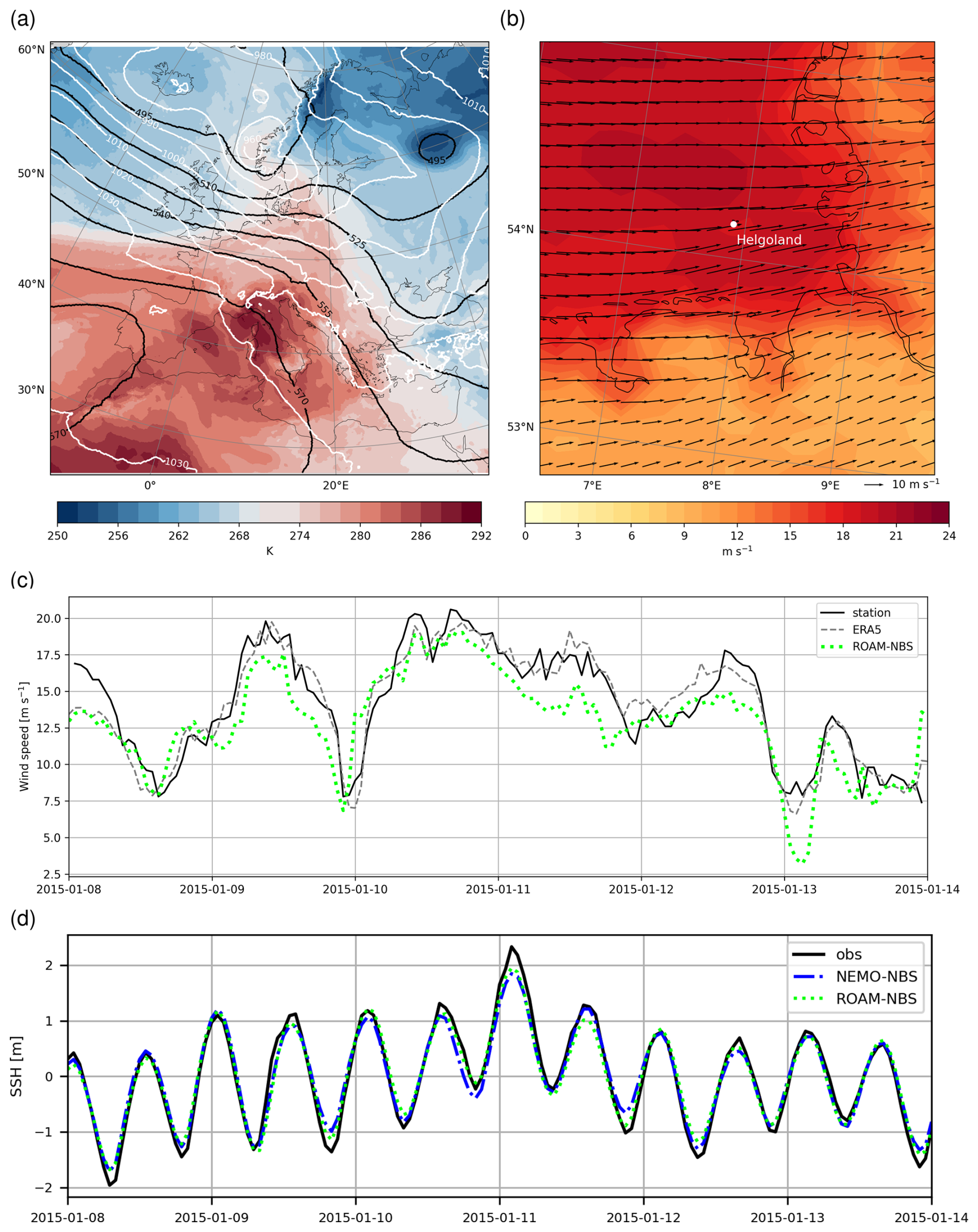
Figure 16 Map for 10 January 2015, 12:00 UTC, displaying isolines of geopotential at 500 hPa (black lines), mean sea level pressure (white lines) and temperature at 850 hPa from ROAM-NBS (a); wind vectors and wind speed at 10 m (shading) in a smaller area centered around Helgoland (b); time series of wind speed of the DWD weather station on Helgoland and wind speed of ROAM-NBS and ERA5, all at 10 m above ground (c); and (d) time series of maximum sea surface height (SSH) at Helgoland.

The storm events in January occur shortly after the Major Baltic inflow event in December 2014. The non-detided SSH results are compared against GESLAv3.0 observational data described in Haigh et al. (2023). Stations in the German Bight (Helgoland), Skagerrak (Helgeroa), and Baltic Sea (Travemünde) are chosen to discuss the model's instant behavior exemplarily. Associated time series of the sea level minus the yearly mean sea level are presented in Figs. 16d and A8. At the station Helgoland, the warning level of 2.5 m for a severe storm surge in the North Sea is exceeded on 11 January in the early morning hours. A small time shift can be observed compared to the wind speed maximum on 10 January. The maximum sea level on 11 January is slightly better represented by the coupled model than NEMO-NBS, although wind speed maxima are comparable in ROAM-NBS and ERA5. Further, the coupled model better coincides with the displayed maxima, which fits the results obtained in the scatter plot at Cuxhaven (Fig. 13). The better representation of the SSH maxima in ROAM-NBS can mainly be attributed to the differences in the treatment of surface boundary conditions, especially the calculation of the wind stress by the surface momentum fluxes (see Sect. 2.3).

In the Skagerrak, again, the maximum sea level for storm events ELON and FELIX in January 2015 is better represented by the coupled model, where some of the minimums in the time series are better represented by NEMO-NBS.

At station Travemünde, no high sea level maximum was present in January 2015. Higher amplitudes around the maximum sea level (4 January) as well as lower sea level values around the sea level minimum (3 January) can be observed for ROAM-NBS in comparison to NEMO-NBS.

4.3 Marine heatwaves

Marine heatwaves (MHWs) are discrete periods of anomalously high SSTs. Following the widely used definition by Hobday et al. (2016), MHWs are identified as periods of at least five consecutive days during which temperatures exceed the 90th percentile of a baseline climatology. To detect MHWs in data and model output, we apply the open-source Python package developed by Oliver (2016) to SST data.

To evaluate model performance in terms of reproducing extreme events, we compare three standard MHW metrics – the annual number of events, the maximum intensity, and the total number of MHW days per year – across four datasets: the two model configurations, in-situ observations, and reanalysis data from Copernicus at two locations. The locations are chosen based on the availability of long-term (>30 years) observational data. One station is in the western Baltic Sea (station Leuchtturm Kiel, 10.27° E, 54.4° N) and one in the German Bight (station UFS Deutsche Bucht, 7.45° E, 54.17° N); see also Fig. 8a for their locations. All MHW metrics are computed relative to each dataset's own climatology, using the common baseline period from 1993 to 2020. Figure A10 in the Appendix compares the seasonal climatology and corresponding 90th percentile threshold across datasets for the station Leuchtturm Kiel. While the model shows a small cold bias in this region, the MHW detection is not affected by this, as it is performed relative to each dataset's individual climatology. Figure 17 presents a comparative analysis of annual MHW metrics at Leuchtturm Kiel derived from in-situ observations (black), reanalysis data (orange), and the two NEMO model configurations: NEMO-NBS (blue) and ROAM-NBS (green), spanning the period 1989–2020. Figure 17a shows the annual number of MHW events, Fig. 17b illustrates the maximum intensity of MHWs (in °C) in each year, and Fig. 17c displays the total number of MHW days per year. The same MHW evaluation is presented in Fig. A9 for the location UFS Deutsche Bucht.

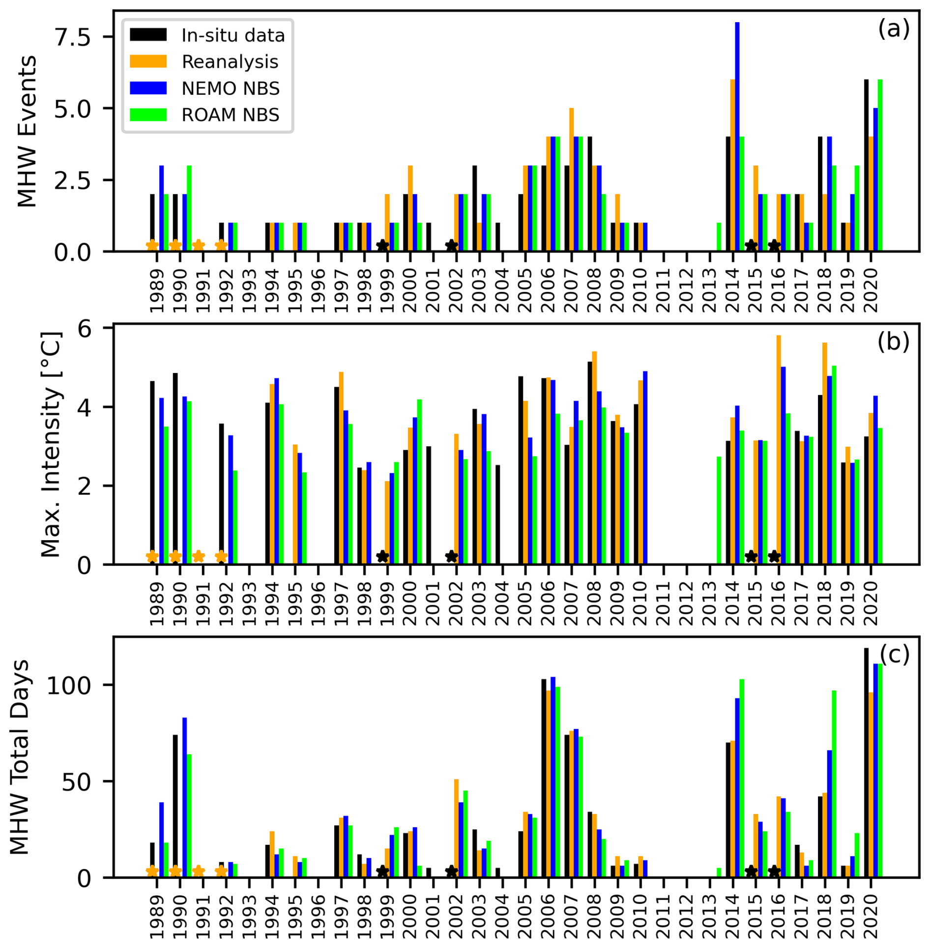
Figure 17 Annual marine heatwaves metrics computed for the location Leuchtturm Kiel in the western Baltic Sea from in-situ data at 0.5 m depth (black), Copernicus Baltic Sea Physics reanalysis data (orange), NEMO NBS simulation (blue) and ROAM NBS simulation (green). Common climatology period is 1993 to 2020. The metrics compared here are number of MHW events (a), maximum intensity [°C] (b) and total days of MHW conditions (c). The orange stars indicate the years where reanalysis data is not available, which starts in 1993. The black stars indicate years with too large data gaps in the in-situ data (1999, 2002, 2015, 2016).

Overall, all model configurations capture the inter-annual variability in MHW characteristics reasonably well at both locations. The NEMO-NBS (blue) generally aligns a little more closely with the observational data in terms of event frequency, maximum intensity, and duration, particularly in recent years. At Leuchtturm Kiel, the NEMO-NBS simulation has a slightly higher Pearson correlation coefficient r with the observed events (NEMO-NBS: 0.85, ROAM-NBS: 0.84), intensity (NEMO-NBS: 0.57, ROAM-NBS: 0.30, i.e. not significant) and MHW days (NEMO-NBS: 0.97, ROAM-NBS: 0.92). However, discrepancies are observed in certain years where model simulations either overestimate or underestimate the magnitude and extent of MHWs. For example, at Leuchtturm Kiel, in 2014 and 2018, both NEMO-NBS and ROAM-NBS tend to overestimate MHW metrics relative to observations, particularly in terms of total days and maximum intensity.

Despite some variability, the model simulations demonstrate skill in reproducing the temporal patterns and intensities of MHWs observed in the region, supporting their application for understanding past and projecting future marine heatwave conditions.

Overall, the evaluation of variability and extreme events shows that both NEMO-NBS and ROAM-NBS can generally reproduce but underestimate the Major Baltic inflow event, that they are able to represent storm surge events, and capture MHWs.

5 Conclusions

Evaluation results from the ERA5/ORAS5-driven evaluation simulation of the coupled regional ocean–atmosphere model ROAM-NBS were presented. ROAM-NBS will be used to produce regional climate projections, which will contribute to the EURO-CORDEX ensemble. Therefore, ROAM-NBS and the simulations with the individual stand-alone versions of the ocean (NEMO-NBS) and the atmosphere (ICON-CLM) were assessed with respect to different observations and reanalyses. NEMO-NBS as well as ROAM-NBS exhibit a small SST bias, which is on area-average about ±0.5 K. For individual seasons and regions, it can also reach larger values. Especially over the Atlantic Ocean, a cold bias prevails for all seasons except summer. In the Baltic Sea, a cold bias prevails. The SST bias is slightly increased in summer in ROAM-NBS compared to NEMO-NBS by about 0.3 to 0.4 K. For both ROAM-NBS and NEMO-NBS, there is no increase in the bias with time throughout the evaluated period of 1979–2020. Warming trends in the North and Baltic Sea are well reproduced by the simulations.

The surface temperature difference against ERA5 exhibits clearly larger values over land than over the ocean. The near-surface air temperature bias over land is overall negative for both ICON-CLM and ROAM-NBS, with a small overestimation of the diurnal minimum temperature and a more pronounced underestimation of the diurnal maximum temperature in all seasons. The temporal evolution of mean temperatures over land is generally in agreement with observational data and reanalyses, with the largest cold bias in Spain and Portugal especially after 1995 and a warm bias in the drier, more continental region of south-east Europe. Differences between ROAM-NBS and ICON-CLM are very small in all land regions and years. Over the ocean, the SST differences between ROAM-NBS and ICON-CLM reflect the bias of NEMO-NBS. The sign of the SST difference coincides with the sign of the differences for sensible and latent heat flux, wind speed, and precipitation, i.e. in regions and seasons where the SST is higher in ROAM-NBS than in ICON-CLM, also the heat fluxes, wind speed, and precipitation are higher, and vice versa. This relationship means that the SST bias introduced into the coupled system by NEMO-NBS influences the atmospheric fields over water, but as shown before, this does not have a systematic influence on the land areas. Compared to station observations, wind speed over the ocean is underestimated, which is slightly more pronounced in ROAM-NBS than in ICON-CLM due to the SST cold bias along the German coast in ROAM-NBS, which causes a reduction of wind speed compared to ICON-CLM. Future improvements in NEMO-NBS could include a time-dependent chlorophyll field that leads to a season-dependent absorption of radiation by the ocean. Improved radiative forcing at the ocean surface could reduce the SST bias in all seasons. Further, a calibration of the lateral and vertical diffusion parameters could enhance the transport over steep ridges in the bathymetry and therefore weaken the salinity bias. In the coupled system, it could be an option to send the ocean albedo over water to the atmospheric part, but then an adaptation in the NEMO coupling interface would be necessary.

The comparison of seasonal mean sea ice concentration between the NEMO-NBS and ROAM-NBS simulations and observational datasets reveals that both simulations tend to overestimate sea ice concentration, particularly during the spring season. While the simulations show good agreement with observations in winter, they significantly amplify sea ice extent in the Gulf of Bothnia during spring. This discrepancy is likely linked to the cold bias and an underestimated salinity in the region. Additionally, the lack of ice dynamics in the current model configurations may contribute to these inaccuracies. Incorporating dynamic ice processes alongside thermodynamic ones and parameter tuning of the thermodynamic ice model may improve the models’ performance and alignment with observed sea ice behavior.

The validation of modeled sea surface salinity (SSS) against observational data from December 1993 to November 2020 reveals consistent spatial patterns and systematic biases in both ROAM-NBS and NEMO-NBS simulations. While surface salinity is generally well captured in the open Baltic Sea and certain coastal regions, persistent underestimations are observed near the Norwegian and German coasts, as well as within the Baltic Sea. Conversely, SSS is overestimated in the transition zone between the Baltic Sea and the North Sea. These biases may be attributed to overly strong prescribed freshwater runoff, which is not exclusively observation-based, and insufficient representation of saline inflow from the North Sea. Prescribing runoff throughout the water column and enhancing vertical mixing could improve sea surface salinity in NEMO-NBS and ROAM-NBS simulations. For the generation of the historical simulations, an online coupled runoff model will be used as in Ho-Hagemann et al. (2024), which is already available in the setup but was not used for better comparability between the coupled and the ocean-only simulation. In deeper layers, both models consistently underestimate salinity, particularly in the Baltic basins, although the surface layers show good agreement with observations. The major inflow events are qualitatively reproduced but quantitatively underestimated. Overall, while the models effectively capture large-scale salinity patterns and seasonal behavior, further refinement of boundary conditions and freshwater forcing is necessary to improve deep water salinity representation and coastal accuracy.

The comparison of mean temperature and salinity profiles from the ROAM-NBS and NEMO-NBS simulations against in-situ observational data reveals both strengths and limitations in the models' ability to reproduce stratification in the Baltic Sea. While both simulations capture surface conditions well across most stations, discrepancies become more apparent at depth. ROAM-NBS exhibits a notable cold and fresh bias in bottom waters, especially in deeper basins like Gotland Deep. For future simulations with NEMO-NBS or ROAM-NBS, longer spin-ups of at least 10 years for the ocean component shall be applied to enhance simulation results. Additionally, it is suggested to apply a bias correction of salinity in the deeper layers of the Baltic Sea (below about 40 m). Surface salinity, however, is generally well represented. NEMO-NBS often achieves lower overall temperature and salinity biases. These findings suggest that while coupled atmosphere–ocean modeling, as in ROAM-NBS, offers advantages for capturing specific vertical structures, future work should focus on improving the ocean component's ability to model inflow events into the deep basins. Furthermore, as mentioned above, a calibration of diffusion parameters will be necessary.

The comparison of model simulations with GESLAv3.0 observational data for the period from January 2015 to December 2019 shows a generally strong agreement in sea surface height (SSH) and storm surge accuracy. After bias adjustment and detiding, the NEMO-NBS simulation shows a slightly better correlation with observations across most evaluated stations than the ROAM-NBS simulation. However, ROAM-NBS tends to capture extreme values more effectively, particularly maxima in the German Bight and Kattegat/Skagerrak regions, suggesting enhanced wind forcing during storms through atmosphere–ocean coupling. A detailed investigation of a storm surge event demonstrates that both NEMO-NBS and ROAM-NBS can reproduce such events properly.

By comparing key marine heat wave (MHW) metrics across observations, reanalyses, NEMO-NBS, and ROAM-NBS, we find that both simulations capture inter-annual variability well, with NEMO-NBS showing slightly better alignment with observations in recent years. Although some overestimations occur in specific years, particularly for intensity and duration, the overall strong correlations support the models' ability to simulate MHW dynamics.

Overall, the coupled simulation ROAM-NBS provides satisfactory results for both the ocean and the atmosphere when compared to observations and reanalysis-driven stand-alone simulations. Therefore, it can be applied to compute regional climate projections for Europe and further deliver climate adaptation information for German national waters. For further applications, it is noteworthy that biases prevail particularly in the Baltic Sea. Since ROAM-NBS does not depend on surface boundary conditions from regional climate projections, unlike NEMO-NBS, CMIP6 information can be downscaled more efficiently when using the coupled model. Moreover, the regional coupled climate projections will also be beneficial for the atmosphere, as the ocean part of ROAM-NBS delivers higher resolved and probably more accurate information at the surface of the North and Baltic Sea than CMIP6 global climate projections.

Appendix A: Complementing evaluations

A1 Mean meteorological conditions

As mentioned in Sect. 3.1, a cloud cover tuning is applied in ICON-CLM to reduce an overestimation of downward shortwave radiation at the surface. The seasonal mean surface shortwave net radiation bias against a satellite product (CERES) is shown in Fig. A1a. After the tuning, it is not much larger than ±10 W m⁻¹. Largest values can be observed in summer (JJA). As the tuning was not location-dependent, it was not possible to decrease the bias further. Additionally, the seasonal surface longwave net radiation bias against CERES is shown in Fig. A1c. The magnitudes of the longwave and shortwave biases are comparable. However, the patterns are different, with the longwave biases reflecting also surface temperature biases, as, for example, too warm land surfaces in south-east Europe in summer. Too high surface temperatures cause an overestimation of upward longwave radiation and, thus, a negative longwave net radiation bias. Over the ocean, the longwave net radiation bias is small (below 10 W m⁻²) most of the time and not larger in summer than in the other seasons, despite the warm SST bias. However, the SST warm bias over the Atlantic ocean in summer is small compared to the surface temperature bias over land, and the cloud cover tuning in ICON-CLM was strongest in summer. More clouds generally increase the longwave net radiation. Finally, high surface temperatures over northern Africa in combination with a less negative (or even positive) longwave net radiation bias can be explained by the influence of aerosols. Aerosols like mineral dust can cause a heating over the whole profile of the troposphere and, thus, increase downward longwave radiation.

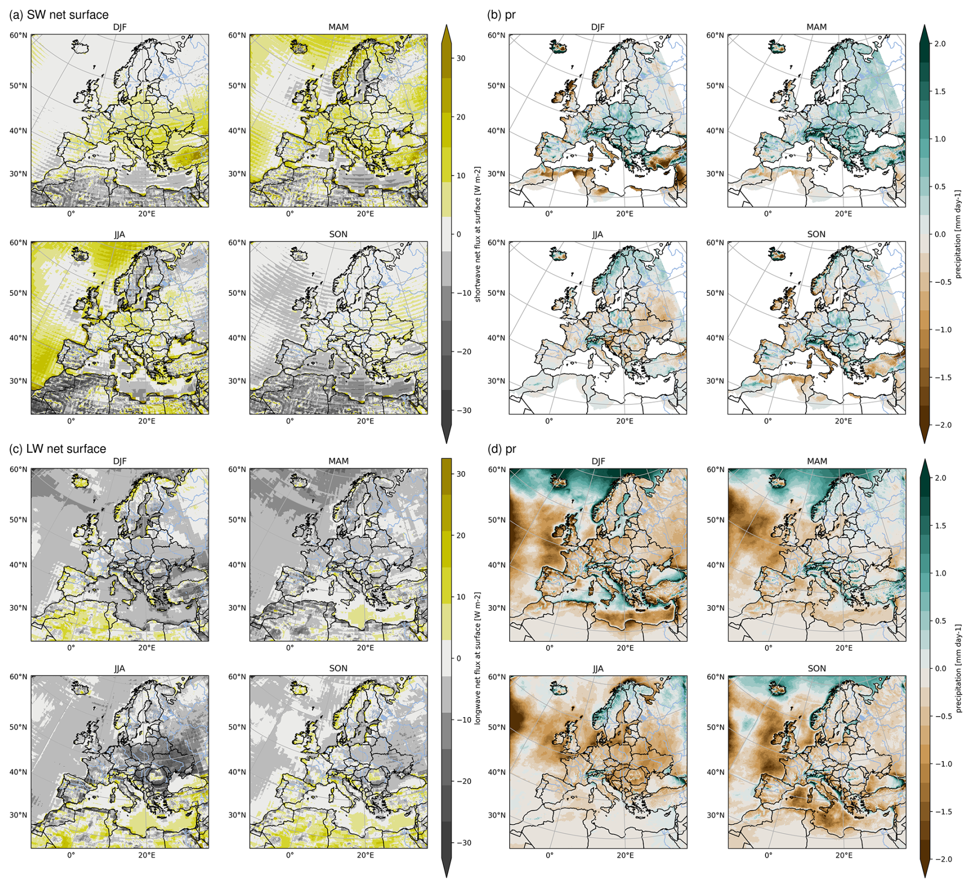
Figure A1 Seasonal mean biases of surface shortwave net radiation for ROAM-NBS against CERES (a), of precipitation against E-OBS (b), of surface longwave net radiation against CERES (c), and of precipitation against IMERG (d), all averaged over 2001–2020.

To quantify the absolute precipitation bias of ROAM-NBS, the mean seasonal biases against E-OBS and GPM (IMERG Final Run v07, Huffman et al., 2023) are given in Fig. A1b and d, respectively. In comparison, the differences between the two simulations (Fig. 6a) are very small (note the differing color scale, which was adapted in Fig. A1b to match the one of the GPM comparison, Fig. A1d). The comparably small simulation difference shows that the ocean coupling only has a small influence on the mean atmospheric conditions.

The precipitation biases against E-OBS are clearly smaller than against GPM, and it can be assumed that E-OBS is more realistic as it is a station-based dataset particularly generated for Europe, while GPM is a global synthesis of multi-satellite precipitation estimates and stations. Still, GPM provides, in contrast to E-OBS, precipitation estimates for the ocean regions. Also over the ocean, the observation bias (Fig. A1d) is much larger than the differences between the simulations (Fig. 6a). Especially in winter, the coupling slightly increases the negative precipitation bias, related to the negative SST bias of NEMO-NBS and ROAM-NBS and, with that, decreased evaporation in ROAM-NBS (see Sect. 3.2.2), but the effect is small. The tuning of evaporation by laminar resistances over the ocean can increase precipitation and was found to be beneficial for most biases over land, but it was disregarded as it resulted in a strong overestimation of evaporation over the ocean compared to satellite observations. In the future, an increase of precipitation efficiency over the ocean should be tested.

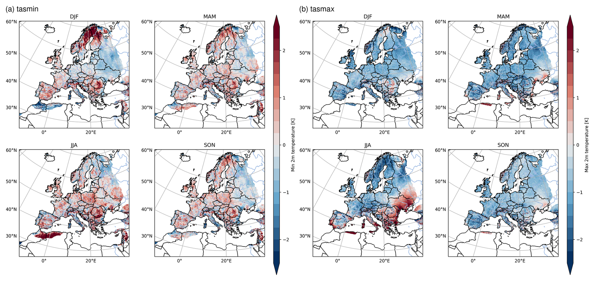
Figure A2 Seasonal mean biases of daily minimum and maximum temperature of ROAM-NBS against E-OBS, averaged over 1979–2020.

Complementing Fig. 5, the seasonal bias maps for ROAM-NBS against E-OBS are shown in Fig. A2 for tasmin and tasmax. They confirm that the tasmin bias is small and non-systematic compared to the more systematic cold bias for tasmax. One slightly outstanding pattern in the tasmin bias is red pattern in Scandinavia in winter (DJF). However, it is unclear if this also might be over-emphasized by the comparison against E-OBS as it does not show up that clearly when comparing against ERA5 (not shown).

To give an insight into the temporal evolution of temperatures within the evaluation period, time series of yearly averaged tas are given in Fig. A3 for different countries. In some cases, neighbouring countries were combined into one time series (GB and Ireland, Spain and Portugal, Norway and Sweden, and the Baltic states including Estonia, Latvia and Lithuania). In general, both ICON-CLM and ROAM-NBS reproduce the mean trends as well as the year-to-year variability of the references (E-OBS and ERA5) very well. As shown before, a cold bias can be discerned which is largest in Spain and Portugal and also clearly visible for GB and Ireland. In the eastern part of the domain, e.g. in Ukraine, the summertime warm bias is dominant. In all cases, ROAM-NBS and ICON-CLM are very similar.

A2 Mean ocean conditions

To complement the evaluation of SST bias evolution in winter and summer, biases and absolute time series for SST integrals over the same regions (whole domain, Open Atlantic, North Sea, Baltic Sea) are presented for all seasons in Fig. A4. In support of the mean profile validation of salinity and temperature, a Hovmöller diagram is provided in Fig. A5, to illustrate the temporal evolution of these variables at stations SMHIBY5 and SMHIBY15. See Fig. 10a for the locations of the stations. Corresponding time series of surface and bottom salinity at stations SMHIBY2, SMHIBY5, and SMHIBY15 are provided in Fig. A6. Furthermore, extending the analysis of detided sea surface height (SSH), Fig. A7 presents a scatter plot comparison of bias-adjusted SSH at the tidal station Plymouth for NEMO-NBS versus ROAM-NBS. Both model configurations exhibit very high correlation with the GESLAv3.0 observational dataset.

A3 Variability and extremes

Time series within the same time period as reviewed in Sect. 4.2 are provided for two additional stations: Helgeroa and Travemünde. The results show a good agreement of ROAM-NBS and NEMO-NBS in the Skagerrak and Baltic Sea, where the maximum SSH is better represented by ROAM-NBS at Helgeroa, whereas at Travemünde the SSH maximum is overestimated by both NEMO-NBS and ROAM-NBS with a slightly better fit by NEMO-NBS. The marine heatwaves are additionally evaluated in Fig. A9 at the station UFS Deutsche Bucht to assess NEMO-NBS's and ROAM-NBS's performance in the North Sea. In Fig. A10, the seasonal climatology and corresponding 90th percentile threshold are presented for ROAM-NBS, NEMO-NBS, the Copernicus reanalysis and in-situ observation data for the station Leuchtturm Kiel.

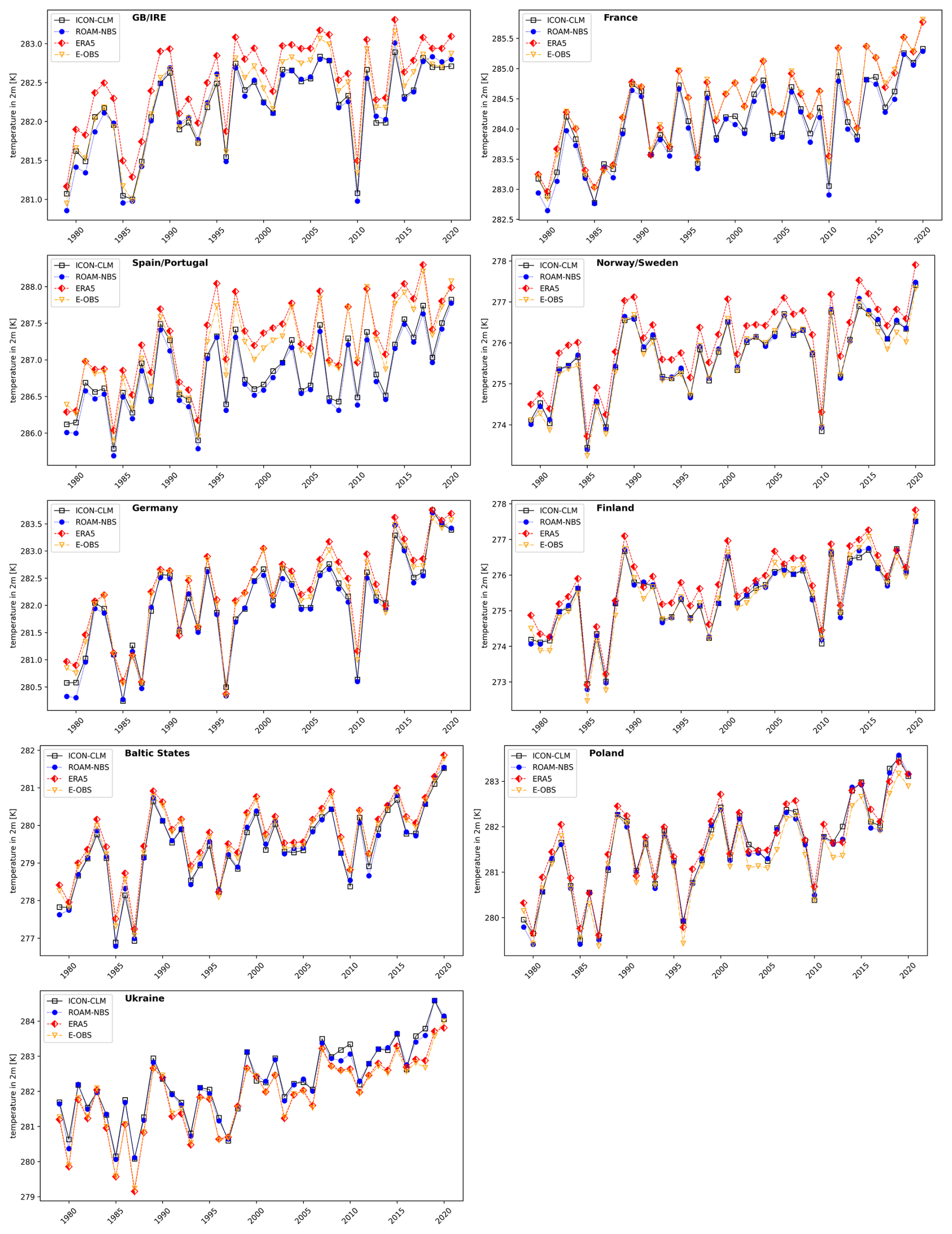
Figure A3 Yearly time series of tas for different countries/regions for ROAM-NBS, ICON-CLM, E-OBS and ERA5.

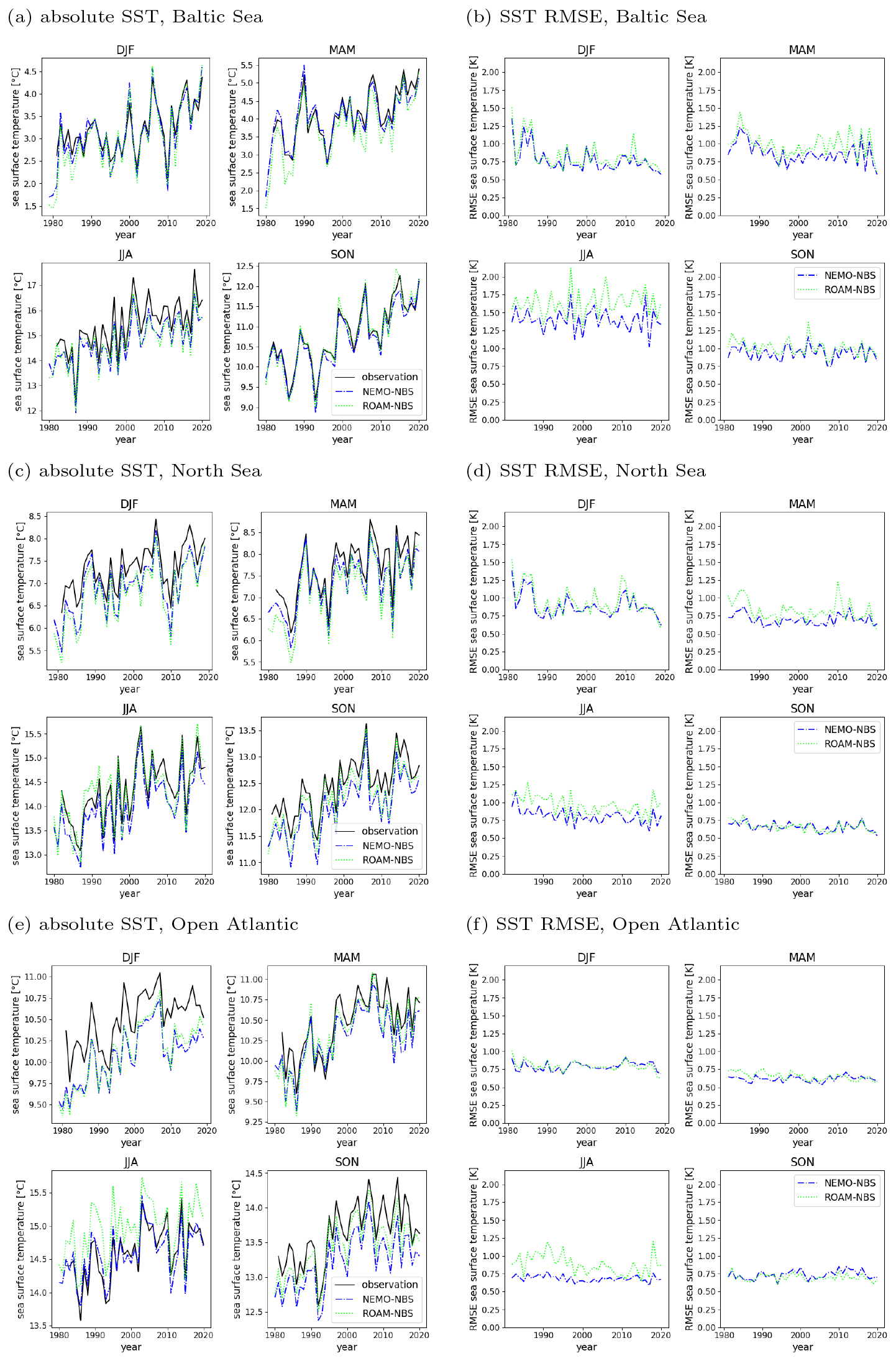
Figure A4 Seasonal mean area-mean SST time series for NEMO-NBS, ROAM-NBS, and Copernicus observation data for the years 1981–2020 for the Baltic Sea (a), the North Sea (c), and the Open Atlantic (e). Difference of seasonal SST time series for NEMO-NBS and ROAM-NBS, respectively, to Copernicus observation data for the Baltic Sea (b), the North Sea (d), and the Open Atlantic (f).

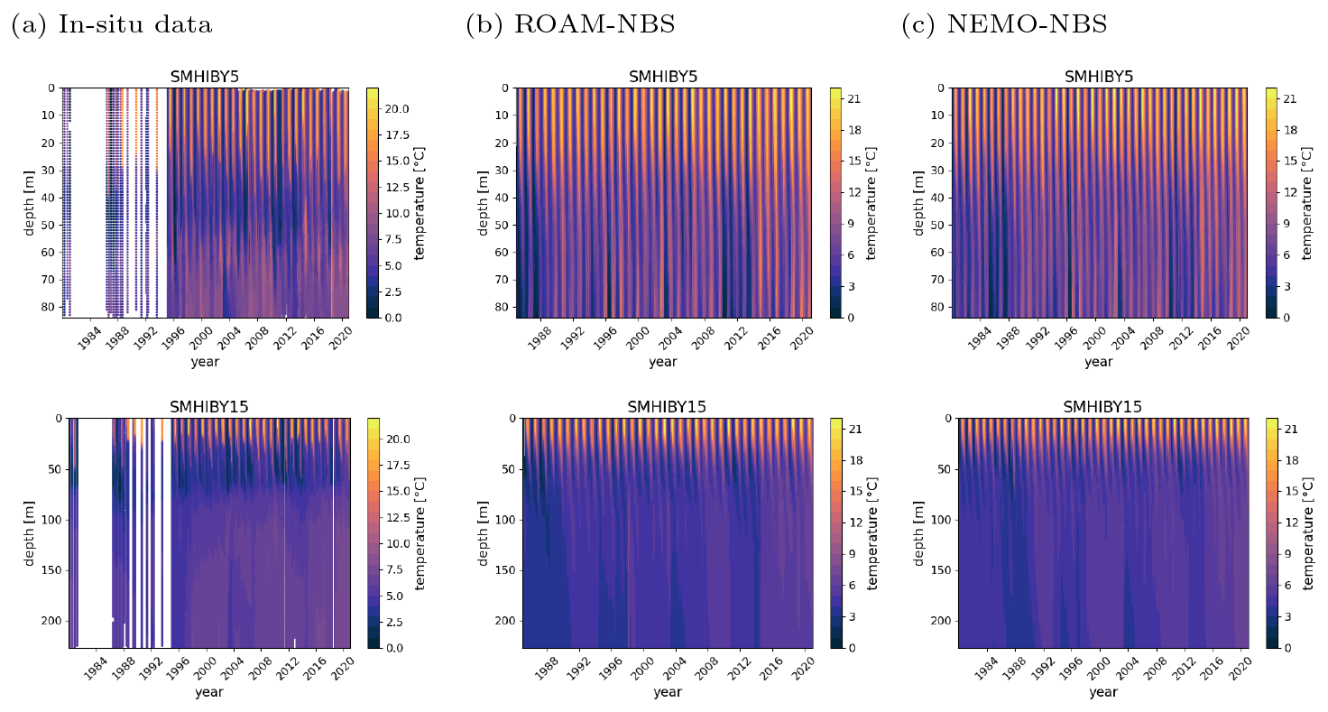
Figure A5 Observed (a) and simulated temperature – ROAM-NBS (b) NEMO-NBS (c) – as a function of depth and time at the monitoring stations Bornholm Deep  (SMHIBY5) and Gotland Deep (SMHIBY15).

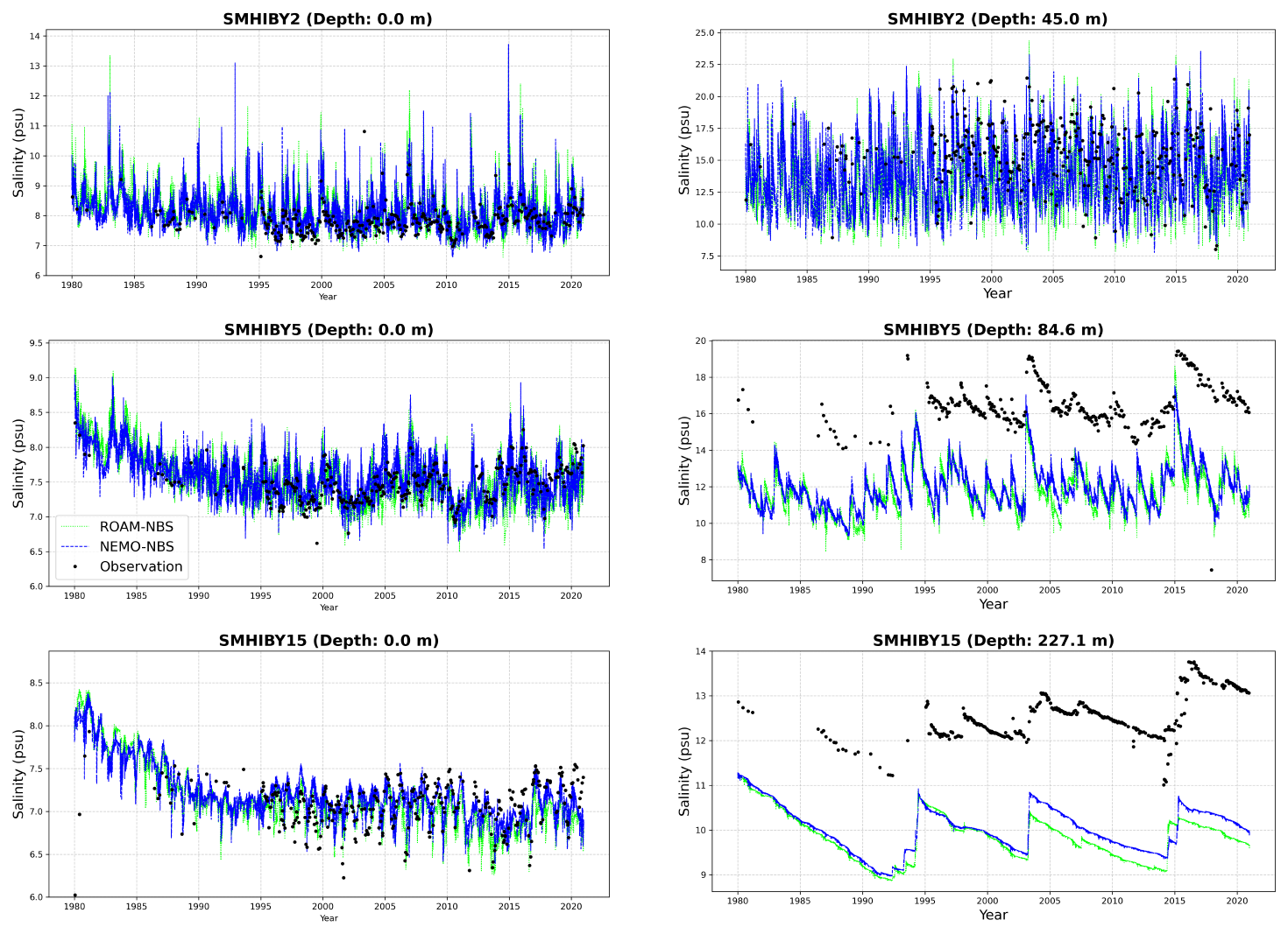
Figure A6 Surface and bottom time series of observed and simulated salinity at Baltic stations (SMHIBY2, SMHIBY5, SMHIBY15).

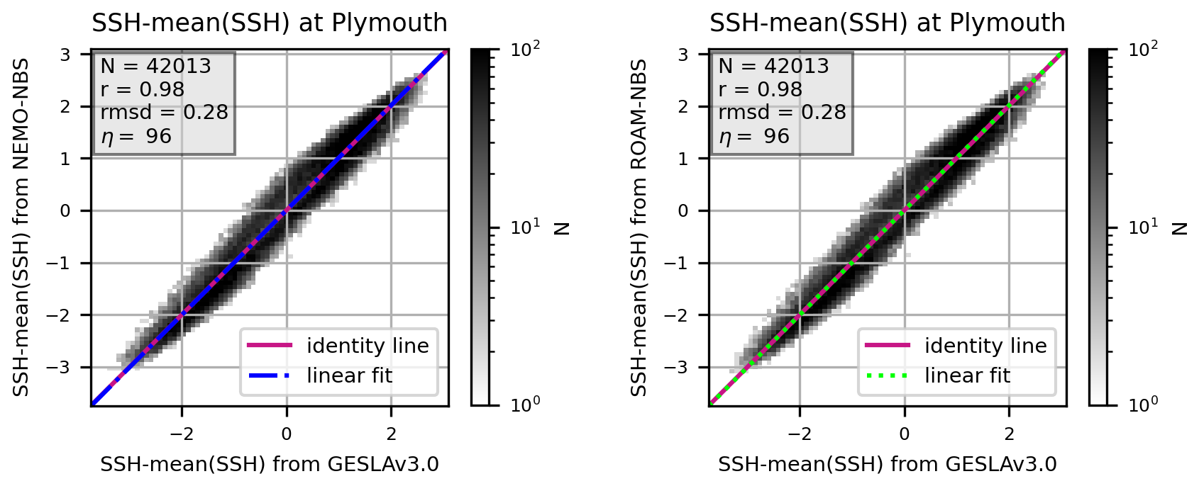
Figure A7 Comparison of exemplary scatter plots of bias adjusted sea surface height at a station in a tidal area (Plymouth) for NEMO-NBS (left panel) and ROAM-NBS (right panel).

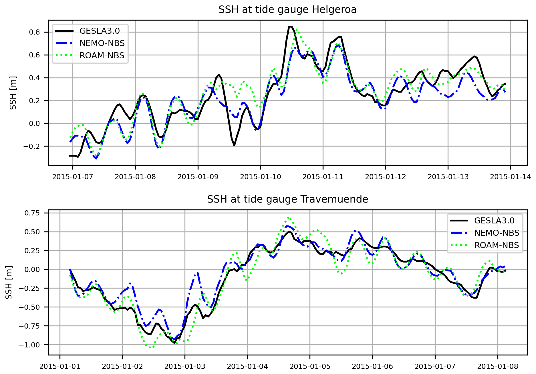
Figure A8 Comparison of model results and observations for maximum sea surface height in January 2015 at selected stations in the Kattegat and Baltic.

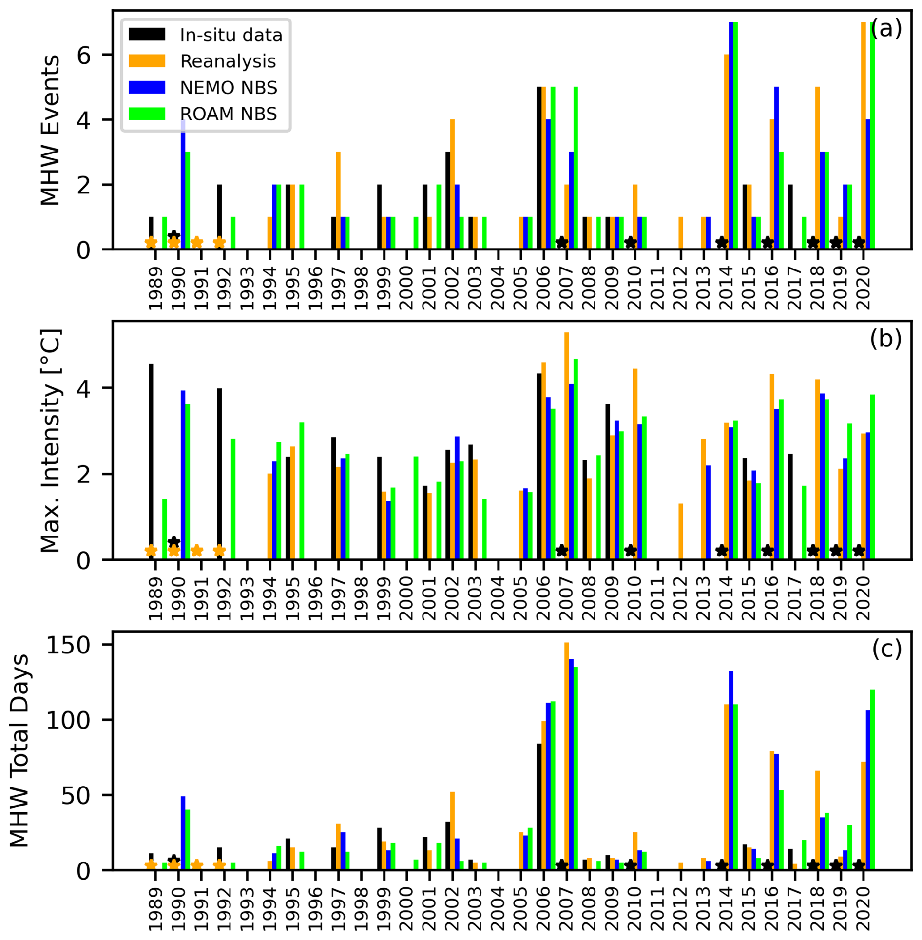
Figure A9 Annual marine heatwaves metrics computed for the location UFS Deutsche Bucht in the North Sea from in-situ data at 0.5 m depth (black), Copernicus Atlantic – European North West Shelf – Ocean Physics reanalysis data (orange), NEMO NBS simulation (blue) and ROAM NBS simulation (green). Common climatology period is 1993 to 2020. The metrics compared here are the number of MHW events (a), maximum intensity [°C] (b) and total days of MHW conditions (c). The orange stars indicate the years where reanalysis data is not available, which starts in 1993. The black stars indicate years with too large data gaps in the in-situ data (1990, 2007, 2010, 2014, 2016, 2018, 2019, 2020).

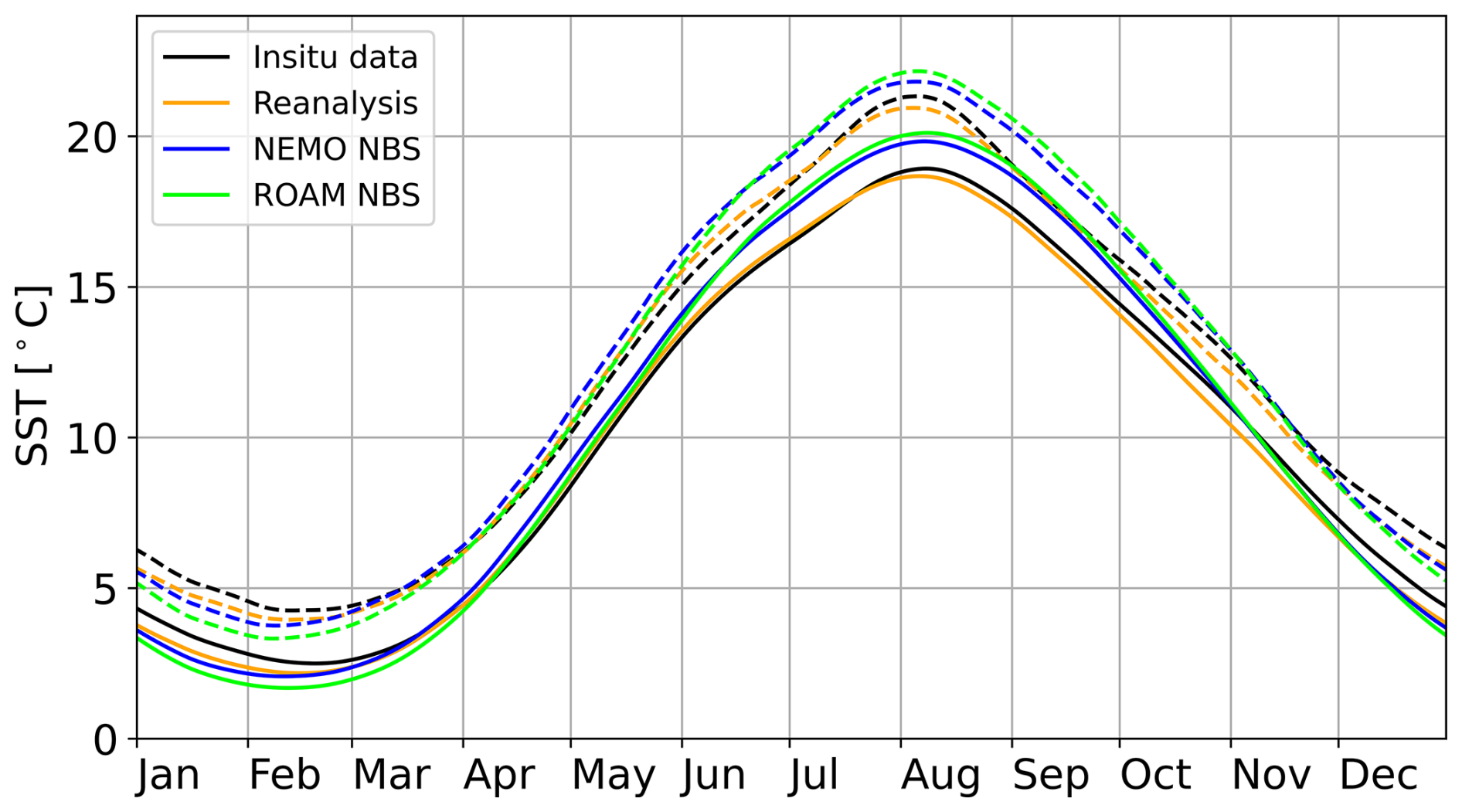
Figure A10 Seasonal climatology (continuous) and corresponding 90th percentile threshold (dashed) computed for the location Leuchtturm Kiel in the western Baltic Sea from in-situ data at 0.5 m depth (black). NEMO-NBS simulation (blue) and ROAM-NBS simulation (green) and Copernicus Reanalysis (orange). Common climatological period is 1993 to 2020.