the Creative Commons Attribution 4.0 License.
the Creative Commons Attribution 4.0 License.
 | 08 Jan 2026
Modeling supercritical CO2 flow and mineralization in reactive host rocks with PFLOTRAN v7.0
Katherine A. Muller
Glenn Hammond
Xiaoliang He
Peter Lichtner
Understanding the flow and reactivity of CO2 injected into geological reservoirs is important for many subsurface applications including secure geologic carbon storage (GCS), critical mineral extraction, enhanced geothermal systems (EGS), and enhanced oil recovery (EOR). Traditionally, subsurface CO2 injection for GCS applications has focused on geologic formations with favorable subsurface configurations for CO2 migration and trapping through non-reactive mechanisms such as structural, solubility, and petrophysical trapping. Recently, CO2-reactive rocks such as mafic and ultramafic basalts have been investigated for their potential to react with injected CO2 in situ to simultaneously dissolve host rock minerals and mineralize CO2 as carbonates. Engineering rapid CO2 mineralization in the subsurface is attractive because of the increased density of stored CO2, the additional safety factors associated with solidification, and the potential to extract valuable critical minerals. Here we present recent developments in the parallel flow and reactive transport simulator PFLOTRAN to model coupled CO2-brine flow and reactive transport for a wide range of injection and production applications involving reactive CO2-brine systems. These developments are based on the well established and trusted CO2 flow capabilities in the STOMP-CO2 simulator. New capabilities added to PFLOTRAN include new CO2-brine equations of state with optional thermal coupling, several new constitutive relationships like capillary pressure smoothing and scanning path hysteresis, a fully implicit well model, and native linkage with PFLOTRAN's well-established reactive transport libraries. A series of benchmarks between PFLOTRAN and STOMP-CO2 verify the newly developed CO2-brine flow capabilities. Demonstrations of coupled CO2-brine flow modeling and reactive transport show how CO2 mineralization can be engineered in reactive host rocks. Finally, an example use case involving copper leaching by CO2 and critical mineral extraction is presented to showcase the strengths of this new implementation. Several limitations still remain, including limited availability of field data to parameterize models. Future work should constrain the evolution of mineral surface area during mineralization and the temperature and/or pH dependence of geochemical reactions for specific systems of interest.
- Article
(8877 KB) - Full-text XML
- BibTeX
- EndNote


Subsurface CO2 injection has been studied for several decades for its potential utility to a variety of subsurface energy applications, including enhanced oil recovery (Sambo et al., 2023) and geologic carbon storage (Bashir et al., 2024). If not properly contained, injected CO2 can also potentially become an environmental contaminant (Harvey et al., 2013). More recently, CO2 has been proposed as a potential working fluid for extracting geothermal energy from conventional and enhanced geothermal systems (Pruess, 2008; Wu and Li, 2020). It has also been shown that in highly CO2-reactive reservoirs composed of, e.g., mafic and ultramafic basalts, CO2 can mineralize as carbonates on much shorter timescales than in traditional non-reactive reservoirs (McGrail et al., 2017; Pogge von Strandmann et al., 2019). The geochemistry of these reactions is also such that the dissolution of the host rock that is promoted by enhanced brine acidity could release valuable critical minerals. CO2 has therefore been proposed as a working fluid to promote critical mineral recovery with the added benefit of storing carbon (Stanfield et al., 2024).
To predict the transient behavior of CO2 injected into the subsurface for any of these applications and to engineer optimal injection strategies, reservoir simulation tools are required. Such tools have matured over the past few decades; recently, the Society of Petroleum Engineers (SPE) concluded its 11th international Comparative Solution Project, which benchmarked state-of-the-art industry and research simulators on a series of CO2 storage challenge problems in 2D and 3D (Nordbotten et al., 2024, 2025). However, many of these tools are limited in their capacity to model coupled multiphase flow and reactive transport in reactive host reservoirs. Lacking these capabilities makes it difficult to predict the long term behavior of a commercial-scale CO2 injection into a reactive host rock, let alone model enhanced critical mineral dissolution and extraction using CO2 as the working fluid.
The parallel flow and reactive transport simulator PFLOTRAN is a state-of-the-art, open-source computational framework designed to simulate subsurface fluid flow, heat transfer, and reactive transport processes for geological research applications ranging from environmental science to energy systems (Hammond et al., 2014). In this work, PFLOTRAN has been extended to model coupled CO2-brine flow and reactive transport for a wide range of injection and production applications involving reactive CO2-brine-mineral systems. These developments are based on the well established and trusted CO2-brine flow capabilities in the STOMP-CO2 simulator (White et al., 2012). New capabilities added to PFLOTRAN include new CO2-brine equations of state with optional thermal coupling, several new constitutive relationships like capillary pressure smoothing and scanning path hysteresis, a fully implicit well model, and native linkage with PFLOTRAN's well-established reactive transport libraries. We first present the theory behind all of this newly-implemented functionality. Then we present a suite of benchmark exercises and verification tests to demonstrate how our implementation compares to other well-established multiphase flow simulators STOMP-CO2 and TOUGH2 (Pruess et al., 1999). Finally, we demonstrate these new capabilities on a copper extraction problem using CO2 to induce copper leaching for critical mineral extraction. The objectives of this work are as follows:
-
Develop coupled CO2-brine flow and reactive transport capabilities in the massively parallel flow and transport simulator, PFLOTRAN.
-
Benchmark these new capabilities against the well established simulators STOMP-CO2 and TOUGH2.
-
Highlight a novel use case of these capabilities: a large-scale CO2 mineralization and critical mineral extraction model with a horizontal injection and production well.
Simulating CO2 injection into reactive subsurface reservoirs requires solving systems of nonlinear partial differential equations describing the transport of water, CO2, and salt; heat transfer; and chemical reactions through porous media at large scales. These equations are strongly coupled: for instance, the dissolved concentration of CO2 affects liquid water density, viscosity, enthalpy and pH among other state variables, which in turn affect the transport and reactivity of other species. In PFLOTRAN, SCO2 Mode has been developed to fully implicitly solve a set of “flow” governing equations. Those equations include conservation of water mass, conservation of CO2 mass, conservation of salt mass, conservation of energy, and well mass flux conservation. Water, CO2, and salt components partition between three phases (liquid [aqueous], gas [CO2-rich], and salt precipitate); water is miscible in the CO2 phase, and CO2 and salt are miscible in the aqueous phase. Transport of mass in the SCO2 flow mode occurs as the result of pressure gradients within each phase, concentration gradients within each phase, buoyancy, and component sources/sinks. These equations are all solved fully implicitly within SCO2 Mode; some equations, like the energy equation and the well equation, are optional. The governing partial differential equations, constitutive relationships, equations of state, and fully implicit well model formulation were designed with base functionality that emulates the STOMP-CO2 simulator and expands beyond those capabilities.
Modeling transport and reaction of dissolved aqueous species also requires solving a coupled system of mass action equations. We refer to this as the “reactive transport” step. To model multicomponent geochemistry in addition to multiphase CO2-brine flow, PFLOTRAN's SCO2 flow mode has been designed to sequentially couple to PFLOTRAN's global implicit reactive transport (GIRT) mode, a mature and comprehensive reactive transport code (Hammond et al., 2014). SCO2 Mode first solves its set of governing equations for mass and energy fluxes over a given time step. Then, it passes certain variables like Darcy fluxes, porosity, and gas phase saturation to reactive transport. Reactive transport then takes as many sub-steps as are required to complete one “flow” step. If CO2 is produced or consumed through mineralization reactions in reactive transport, transport passes a source/sink term of CO2 back to flow. Flow and reactive transport hand this information off at every flow time step for the duration of the simulation.
2.1 SCO2 Mode Governing Equations
PFLOTRAN's SCO2 Mode solves a fully coupled system of three component mass conservation equations and one energy conservation equation. The energy conservation equation can be optionally disabled in favor of isothermal simulations at user-defined initial temperature conditions (including temperatures read from a restart file). Additionally, an arbitrary number of fully coupled well mass conservation equations can be solved corresponding to each well in the domain with or without thermal coupling. The default mass and energy conservation equations consider conservation of water, CO2, salt, and system internal energy. The equations take the following form:
where ϕ is porosity, sα is the saturation of phase α, ρα is the mass density of phase α, is the mass fraction of component β in phase α, qα is the Darcy flux of phase α, is the diffusive flux of component β in phase α, qβ are the sources and sinks of component β, Uα is the internal energy of phase α, is the heat capacity of the rock, ρrock is the solid rock density, T is temperature, Hα is the enthalpy of phase α, κeff is the effective thermal conductivity of the medium, and qe are the energy sources and sinks.
Three phases are considered in this formulation: aqueous phase, CO2-rich phase, and salt precipitate phase. Within the CO2-rich phase, trapped and free-phase saturations are tracked separately for performing optional hysteresis calculations. The salt precipitate phase contains only the salt component; the salt component can also partition into the aqueous phase, but it cannot exist in the CO2-rich phase. The state of the CO2-rich phase can be either liquid, gaseous, or supercritical CO2. The CO2-rich phase is always treated as a single phase, and its properties are computed directly from the Span-Wagner EOS, which is valid for liquid, gas, and supercritical CO2. A limitation of this approach is that it does not explicitly model an interface within a grid cell where CO2 may be transitioning from, e.g., liquid to gas. For convenience, the CO2-rich phase will be labeled the “gas” phase throughout this document. This phase can contain both CO2 and water components.
2.2 Constitutive Relationships
Advective fluxes of the mobile phases are modeled using Darcy's equation:
where k is the permeability of the medium, is the relative permeability of phase α, μα is the viscosity of phase α, pα is the pressure of phase α, γα is the specific gravity of phase α, and z is vertical elevation. This formulation assumes a laminar flow regime.
Relative permeability is computed as a function of pore fluid saturations through one of several available relative permeability function options. Please see the PFLOTRAN Documentation (https://documentation.pflotran.org, last access: 18 December 2025) for a comprehensive list of available relative permeability functions for liquid and gas phases. When considering effects of hysteresis on gas trapping, SCO2 Mode removes trapped gas from the mobile gas phase saturation used in gas relative permeability computations.
Diffusive fluxes in the aqueous phase are modeled using Fick's Law:
where is the diffusivity of component β in the liquid and ∇cβ is the gradient in dissolved concentration of component β. Transport of dissolved salt through the aqueous phase is additionally weighted using the Patankar method (Patankar, 2018).
Likewise, gas phase diffusive flux is modeled as follows:
where is the diffusivity of component β in the gas and ∇cβ is the gradient in mass fraction of component β in the gas. The salt component is not present in the gas phase.
2.3 Equations of State
Several options exist in PFLOTRAN to customize the set of equations of state (EOS) used in a simulation to fit a desired application. Here we describe the default options available in SCO2 Mode. We refer the user to the PFLOTRAN Documentation (https://documentation.pflotran.org, last access: 18 December 2025) for more information on EOS options.
2.3.1 Density
With the exception of the salt precipitate phase, the composite density of each phase is computed by correcting the pure phase density as a function of component concentrations. The salt precipitate is considered to be a pure “salt” component phase. The default density equation for salt is a function of temperature and pressure and assumes that salt is composed entirely of NaCl (Battistelli et al., 1997).
For the aqueous liquid (non CO2-rich) phase, the density of pure water is first computed as a function of pressure and temperature (Meyer et al., 1993). Brine density is then computed as a function of pure water density and salt mass fraction (Phillips et al., 1981). Finally, the composite mixture density is calculated as a function of pure water density, brine density, and mass fractions of salt and CO2 components (Alendal and Drange, 2001).
In the gas phase, a similar approach is taken with the exception that there is no dissolved salt in the gas phase. Pure gas phase density (Span and Wagner, 1996) and water vapor density (Meyer et al., 1993) are first calculated as functions of pressure and temperature. Then, the gas mixture density is computed as a weighted average of the two densities weighted by gas phase component mass fractions. Pure CO2 thermodynamic properties (density, viscosity, internal energy, and enthalpy) can either be computed or read in through a database for greater efficiency. A generic CO2 thermodynamic property table based off of the Span-Wagner EOS is included in the PFLOTRAN database directory and it is recommended to use this lookup table for CO2 simulations.
2.3.2 Vapor Pressure
The liquid vapor pressure is computed as a function of temperature, salinity, and capillary pressure. Pure water saturation pressure is first computed as a function of temperature (Meyer et al., 1993), and then an adjustment is applied to include the effect of salinity (Haas, 1976). The Kelvin equation is then applied to calculate the reduced vapor pressure as a function of capillarity (Nitao, 1988).
2.3.3 Viscosity
Similar to density, the viscosity of each mobile phase is computed as a function of temperature, pressure, and phase composition. For the liquid phase, the viscosity of pure water is computed as a function of temperature and pressure (Meyer et al., 1993). This pure water viscosity is then adjusted as a function of temperature and salinity (Phillips et al., 1981) to get the brine viscosity. The viscosity of CO2 is separately calculated as a function of temperature and density (Fenghour et al., 1998), and the final composite liquid viscosity is computed as a function of CO2 mass fraction, CO2 viscosity, and brine viscosity. In the gas phase, viscosity is calculated as a function of pure water viscosity, pure CO2 viscosity, and mass fractions of each component in the gas phase (Poling et al., 2001).
2.3.4 Diffusion Coefficients
Diffusion drives fluxes of dissolved CO2 and dissolved salt in the aqueous phase, and it drives water vapor diffusion in the gas phase. Diffusive flux is governed by concentration gradients and molecular diffusion coefficients of each component in each phase. In the aqueous phase, the diffusion coefficient of CO2 is computed as a function of temperature (Cadogan et al., 2014) and dissolved salt mass fraction (Belgodere et al., 2015). The molecular diffusion coefficient of salt in the aqueous phase is computed using the Gordon method (Poling et al., 2001) and as a function of mean ionic activity (Bromley, 1973). The diffusivity of water vapor in the gas phase is computed as a function of temperature and pressure via the method of Wilke and Lee (Poling et al., 2001).
2.3.5 Two-Phase Equilibrium
When dissolved CO2 exceeds its solubility in the aqueous phase, or when water vapor condenses from the CO2-rich phase, a two-phase state can arise in a model. That is, in a given cell/location, both the liquid (water-rich) and gas (CO2-rich) phases can coexist. In SCO2 Mode, the transition from single- to two-phase is treated as an equilibrium process. Two-phase coexistence therefore requires an equilibrium partitioning model to determine how CO2 and water partition between phases at a given pressure, temperature, and salinity. This equilibrium partitioning is used to determine the solubility of CO2 dissolved in water and the partial pressure of water vapor in the gas; these are used as conditions for determining the transition between the single-phase aqueous state and the two-phase state or the single phase gas state and the two phase state, respectively. At temperatures below 100 °C, the method of (Spycher et al., 2003) is used. Above 100 °C, the method of (Spycher and Pruess, 2010) with salinity correction is used.
2.3.6 Internal Energy and Enthalpy
Enthalpy of the liquid phase is computed as a function of temperature, pressure, dissolved CO2 concentration, dissolved salt concentration, and individual pure component enthalpies (Battistelli et al., 1997). Pure liquid water enthalpy is computed from the pure water EOS (Meyer et al., 1993) and then adjusted as a function of salinity (Michaelides, 1981). Pure CO2 enthalpy is computed from the CO2 EOS (Span and Wagner, 1996). In the gas phase, the composite gas phase enthalpy is computed as a weighted average of water vapor enthalpy and pure CO2 enthalpy, weighted by the mass fraction of each component in the gas. Finally, the internal energy of each phase is computed by taking phase enthalpy and subtracting cell pressure divided by phase density.
2.4 Fluid-Rock Properties
Several fluid-rock properties are computed as functions of the state of the pore fluids in the system. Separate gas phase and liquid phase tortuosities are computed as functions of rock porosity, liquid saturation, and gas saturation (Millington and Quirk, 1959). When dissolved salt mass becomes supersaturated in the aqueous phase, it precipitates as a solid and changes both the effective porosity and the absolute permeability of the medium (Verma and Pruess, 1988). Relative permeability of each mobile phase is computed as a function of phase saturations; when modeling trapped gas hysteresis, the liquid-saturated end point of the gas phase relative permeability model adapts as a function of trapped gas saturation. Optionally, the CO2-brine-rock interfacial tension can be scaled as a function of salt concentration and temperature. This results in a decrease in capillary pressure with decreasing interfacial tension (White et al., 2012).
2.4.1 Unsaturated Capillary Pressure Extensions
At the unsaturated end of a typical capillary pressure function (e.g., Van Genuchten or Brooks-Corey), there can exist a non-zero residual liquid saturation toward which the capillary pressure increases asymptotically. This is due to the fact that drainage of the wetting (aqueous) phase by the non-wetting (gas) phase is limited by the connectivity of the liquid phase in the porous medium. When the liquid phase is completely disconnected, the gas phase is unable to displace any more liquid and therefore capillary pressure can theoretically become infinite. However, under miscible two-phase flow conditions where both the water and the CO2 components can dissolve into both phases, it is possible to drive water saturation below the residual saturation without displacing fluid. In the case of dry CO2 injection, continuous pumping of a pure CO2 phase into a brine-saturated reservoir can cause desaturation of the rock through desiccation, where water molecules evaporate from the liquid phase into the free CO2 phase.
Capturing this phenomenon requires extending the capillary pressure past the residual liquid saturation. Using the approach of Webb (2000), the capillary pressure function is divided into two regimes: above and below the matching point aqueous saturation. The matching point saturation is the point at which the capillary pressure curve transitions between its original form and its extension to low aqueous saturation conditions. The matching point is computed by finding the aqueous saturation at which the slope of the original capillary pressure curve matches that of the extended curve given a specified capillary pressure at zero liquid saturation (i.e., the oven-dried capillary pressure) and a specified extension shape. In PFLOTRAN, several types of unsaturated extensions are available for the standard Van Genuchten capillary pressure model (Paul et al., 2024). Additionally, this work developed a capillary head-based Van Genuchten model with a logarithmic extension (Fayer and Simmons, 1995) and a Brooks-Corey capillary pressure with a logarithmic extension, both of which are compatible with the scanning path hysteresis model.
2.4.2 Gas Trapping Hysteresis
Gas trapping occurs when an aqueous phase imbibes through a medium that is partially saturated with a gas phase. The gas phase can become disconnected and therefore immobilized (though, analogous to the desiccation process, CO2 can continue to dissolve into water and diffuse through the aqueous phase) as aqueous phase saturation increases throughout the medium. The extent to which the free gas phase can be trapped depends on the degree to which the medium was saturated with gas prior to imbibition. The process of gas trapping can therefore be formulated as a hysteretic phenomenon via a scanning path hysteresis model (Parker and Lenhard, 1987). PFLOTRAN implements the simplified Parker and Lenhard formulation to model trapped gas hysteresis (Kaluarachchi and Parker, 1992). This model is compatible with the Brooks-Corey capillary pressure model and the capillary head-based Van Genuchten model, as well as any choice of relative permeability functions.
2.5 Fully Implicit Well Model
An optional fully coupled well model can inject CO2 or produce reservoir fluids in user-specified portions of a model domain and dynamically adapt to changes in pressure along the wellbore, pressure in the reservoir, and physical properties of the formation. The well model is solved on an embedded sub-domain of the reservoir grid; where a well segment passes through a reservoir cell, the associated flux from well to reservoir is incorporated into the residual and Jacobian calculations.
To construct a well, the well trajectory is first defined by the user in terms of line segments and curves. The wellbore is then discretized as a function of the reservoir grid discretization, and finally individual well segments are each coupled to their corresponding reservoir grid cells.
When embedded into a discrete reservoir, a well model is defined in terms of well segments, well segment centers, and the reservoir cell center through which each well segment passes. In Fig. 1, well segments are defined by the intervals between blue circles. Green circles denote the well segment centers, which are defined by their centroids. Red circles denote the center of each reservoir cell through which the well passes.
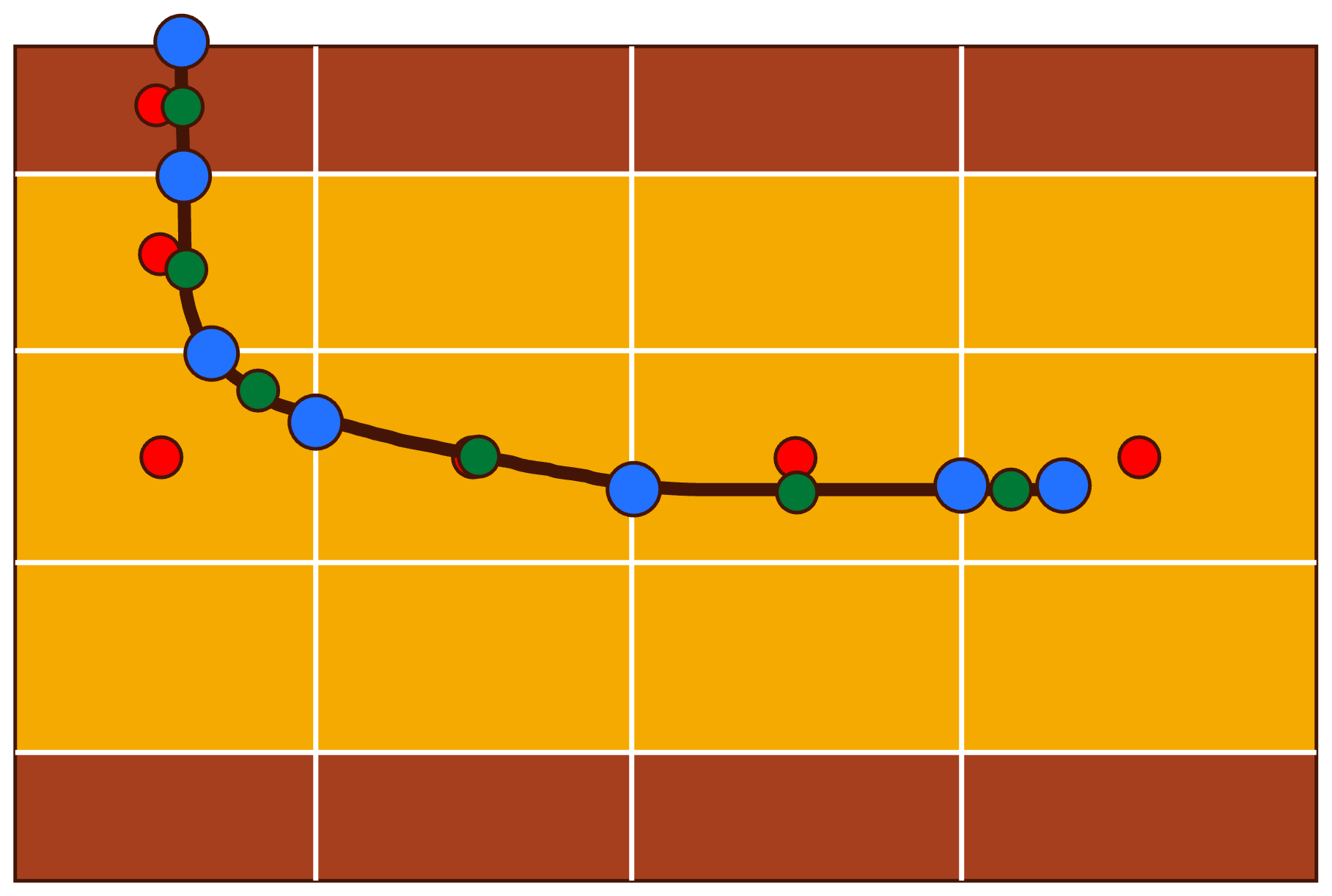
Figure 1Discretized well model embedded in a layered reservoir. Blue dots mark the ends of each well segment, green dots mark well segment centers, and red dots mark reservoir cell centers.
Invoking the well model adds one extra equation to the set of governing equations in the following form:
where Qw is the mass flow rate of phase α between the reservoir and the well in well segment i, and qw is the surface mass flow rate of phase α into or out of the well. The fluid flux in or out of the well at a given well segment is computed as a function of the pressure difference between the center of each well segment and the reservoir cell that the segment occupies, where the cell-centered reservoir pressure is adjusted by a hydrostatic correction to the same depth as the well segment:
where ρα is the density of phase α, μα is the viscosity of phase α, is the wellbore pressure at the center of well segment i, is the pressure in the reservoir cell occupied by well segment i, g is the gravity vector, and zw−r is the vertical offset between well cell center and reservoir cell center. The well index, WI, is computed as a function of the directional permeability of the reservoir in addition to well properties like well orientation, skin factor, casing, and wellbore radius through a modified 3D anisotropic Peaceman equation (Peaceman, 1978, 1983) using the projection of an arbitrarily oriented well segment onto the principal axes of the domain (Shu, 2005; White et al., 2013; Nole et al., 2025a).
In the fully implicit formulation, bottomhole pressure is solved as a primary solution variable in addition to the reservoir primary variables. Wellbore pressure in each segment is then computed as a function of well bottomhole pressure by assuming hydrostatic pressure conditions along the well. Fluid densities in each segment of the well are computed as functions of pressure and temperature; the elevations of well segment centers are fixed at the beginning of a simulation. The hydrostatic well model is numerically efficient but is limited to simulating injection or production only; this model therefore cannot simulate, e.g., cross-flow from one geologic layer to another via the well.
Well pressure control can be imposed individually upon each well either through a specified fracture pressure (injection wells) or through a minimum pressure (extraction wells). Wells are initialized as rate-controlled until the well bottom hole pressure hits either the specified fracture pressure (max pressure) or the minimum pressure. If one of these pressure bounds is exceeded, the well switches to pressure controlled, whereby the pressure in the well is fixed and flow rates are computed accordingly. This can be used to prevent either injection wells from injecting at pressures that would fracture the host rock or extraction wells from generating non-physical suction. Note that when a well is pressure-controlled, the user-specified surface flow rate from Eq. (11) will not be imposed until the well returns to the rate-controlled condition (i.e., the well pressure falls within the user-specified bounds again).
2.6 Primary Variables and Phase States
In addition to modeling miscible coupled flow of CO2-rich and aqueous phases, SCO2 Mode also models phase appearance and disappearance. Depending on the phase state of the system, PFLOTRAN solves its system of governing equations for different primary variables. When phase state changes, those primary variables are also changed accordingly. For example, if a grid cell begins a simulation in the aqueous state, only liquid water, dissolved CO2, and dissolved salt exist in that grid cell. In this state, the primary variables are liquid pressure, CO2 mass fraction, salt mass fraction, and (optionally) temperature. If CO2 is injected into the cell, dissolved CO2 mass fraction increases until it exceeds the solubility of CO2. Once this happens, dissolved CO2 mass fraction becomes fixed and another primary variable must be used to solve the system of equations. The cell therefore transitions to the two-phase state and updates its primary variables. The transition from aqueous to two-phase state requires only one primary variable to change: CO2 mass fraction to gas phase pressure. SCO2 Mode considers four phase states: an aqueous state with no free-phase CO2, a two-phase state with both aqueous and free-phase CO2, a gas state with only free-phase CO2, and a trapped gas state with only aqueous liquid phase and immobile trapped gas phase (Table 1). When designing a model, care should be taken to identify which phase state the grid cells should be assigned at initialization and choose the set of primary variable constraints accordingly (see Sect. A2 for more discussion).
Table 1Primary Variables and Phase States.
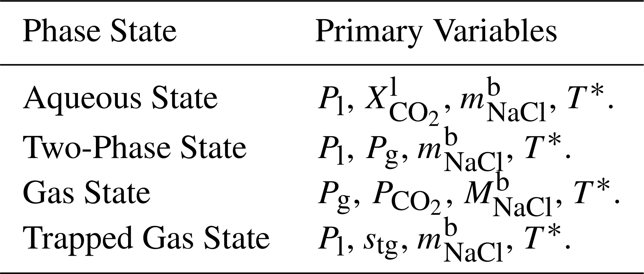
Temperature is only required for thermal models.
2.7 Reactive Transport Governing Equations
PFLOTRAN's reactive transport process model couples multiphase, multicomponent transport and biogeochemical reaction through the governing mass conservation equation:
with porosity ϕ, saturation s, total component concentration ψ, Darcy velocity q, tortuosity τ, hydrodynamic dispersion tensor D, and source/sink term q for primary species j in phase α. Kinetic rates are scaled by the stoichiometry of species j in each reaction r. The total component concentrations for the liquid and gas phases are defined, respectively, as
with aqueous free ion concentration c, secondary aqueous complex concentration χ, and gas concentration Cg. νji and are the stoichiometric contribution of the free ion species j to each secondary aqueous complex and gas.
Secondary aqueous complex and gas concentrations are defined, respectively, by the expressions
through the law of mass action (Lichtner, 1985).
2.7.1 Solubility of CO2 in the Aqueous Phase
Following Duan and Sun (2003), equilibrium is defined as equality of the chemical potential (μ) of CO2 in liquid and gas phases
For multi-component systems where CO2(aq) may not be the primary species for the CO2 component (e.g., use of HCO instead of CO2(aq)), equilibrium is generalized to
where the sum j is over all primary species and is the stoichiometric contribution of each primary free ion species to the secondary CO2(aq) species. Substituting the expressions for the chemical potentials equating liquid and gas potentials
where and are respectively the fugacity coefficient and partial pressure for species i′ in the gas phase. Substituting Eqs. (20)–(21) into Eq. (19) yields
and alternatively,
Or in terms of the gas equilibrium constant
with the equilibrium constant related to the standard state chemical potentials by the equation
and
Substituting Eq. (26) and the exponential of Eq. (25) into Eq. (24) results in
2.7.2 Contribution to CO2 Residual Equation
For grid cells with a nonzero CO2 gas saturation (i.e., sg>0), the governing mass conservation equation (i.e., Eq. 13) for CO2 is replaced by a residual equation that constrains the CO2(aq) concentration against the solubility of CO2. The residual equation for the primary CO2 species (i.e., CO2(aq), HCO or CO) is then based on Eq. (27), i.e.,
with Jacobian entries
where is the residual equation for the CO2 component and j′ represents the primary species.
Five benchmark test cases were built to demonstrate the capability of SCO2 Mode to simulate multiple coupled processes related to subsurface CO2 injection, brine mixing, multiphase miscible flow with hysteresis, well modeling, and reactivity. These models were constructed from STOMP-CO2 short course material (https://stomp-userguide.pnnl.gov/shortcourse_examples/example_problems.html, last access: 18 December 2025) to directly compare PFLOTRAN's results with those produced by STOMP-CO2 (White, 2023).
3.1 Radial Flow of Supercritical CO2
The first benchmark test was designed to evaluate the ability of simulators to properly model two-phase flow of CO2 and brine under capillary and relative permeability effects; to adequately account for temperature, pressure, and salinity dependent phase properties like density, viscosity, and CO2 solubility; and to appropriately handle phase behavior like CO2 bubbling and salt precipitation during desiccation.
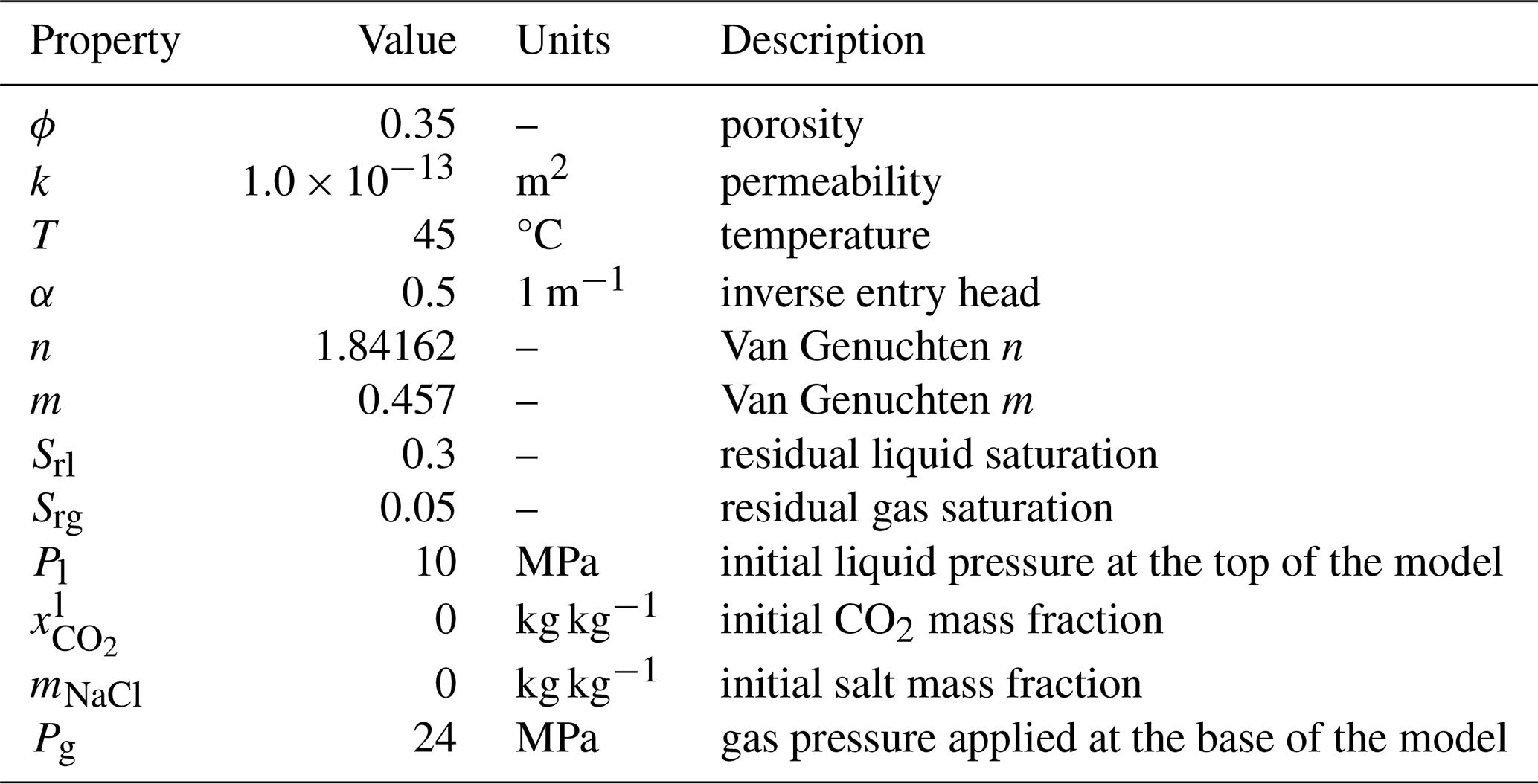
This benchmark problem is equivalent to STOMP-CO2 Short Course Example Problem CO2-1. In this problem, originally developed for the GeoSeq Project (Pruess et al., 2002), a 1D radial domain is initialized to a constant pressure of 12 MPa and a temperature of 45 °C. The domain is initially water-saturated; at the beginning of the simulation a constant supercritical CO2 (scCO2) injection rate of 12.5 kg s−1 is applied at r=0 m and held constant throughout the simulation. The aquifer is homogeneous and isotropic, and the far edge of the model is placed such that the domain is essentially infinite. Gravity effects are ignored.
This problem has two variants: first, the CO2 injection occurs in a freshwater aquifer; second, CO2 is injected into a brine aquifer. Injection is simulated using a simple source term in the first grid cell (not a well model). Table 2 summarizes key properties of the model.
Table 2Radial Flow of Supercritical CO2: Model Properties.
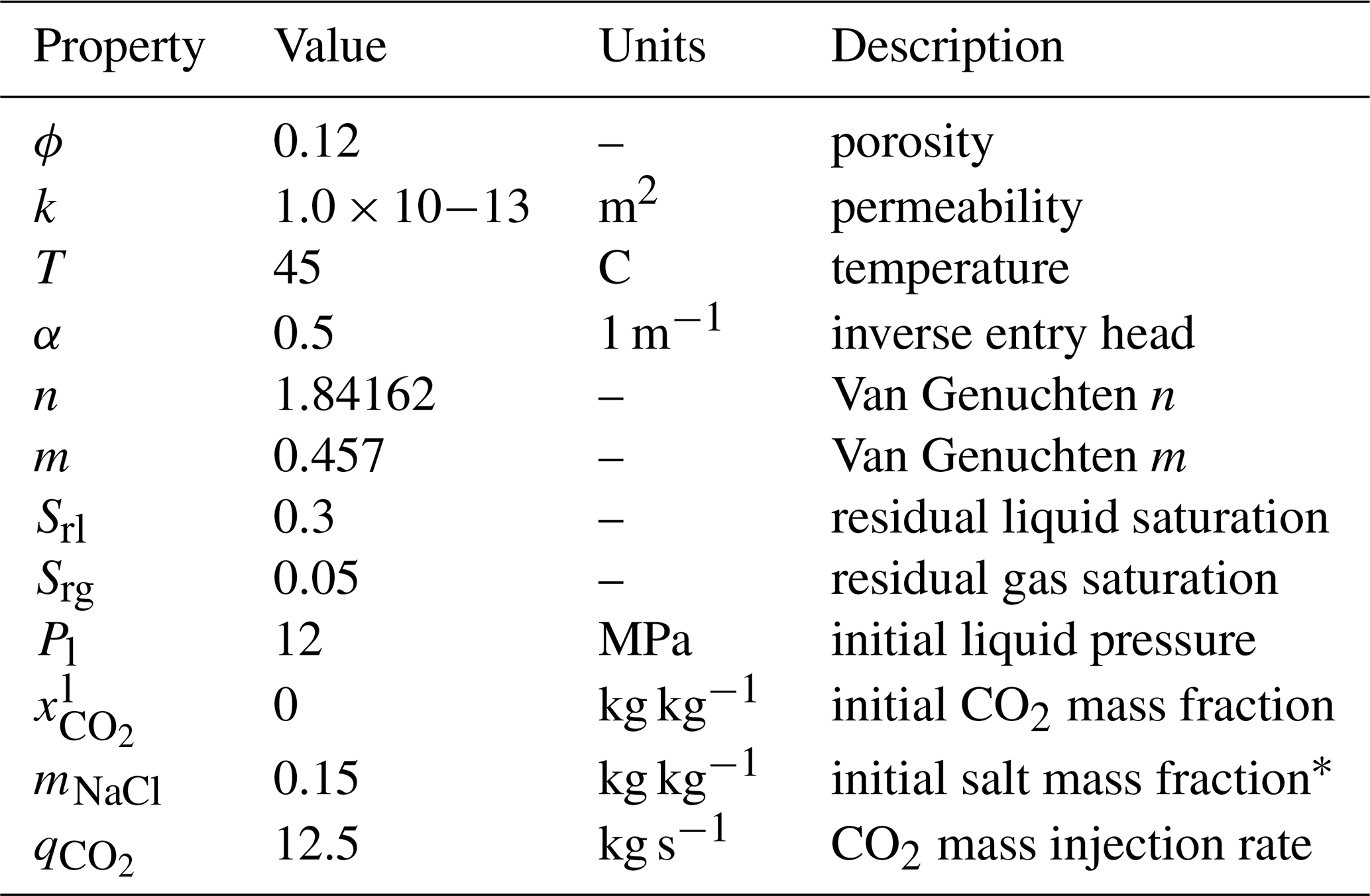
* Salt mass fraction is zero for the first problem variant.
3.1.1 Zero Salinity
In this variant of the Radial Flow of Supercritical CO2 benchmark problem, CO2 is injected into a freshwater aquifer (no dissolved salt). Both PFLOTRAN and STOMP-CO2 simulators were run with the same model setup; plots of a select set of output variables vs radial distance from the wellbore are shown below. These output variables include gas pressure, gas saturation, and dissolved CO2 mass fraction (Fig. 2). For this problem, PFLOTRAN and STOMP-CO2 results are nearly indistinguishable, indicating very strong agreement between the two simulators and verifying the implementation in PFLOTRAN.
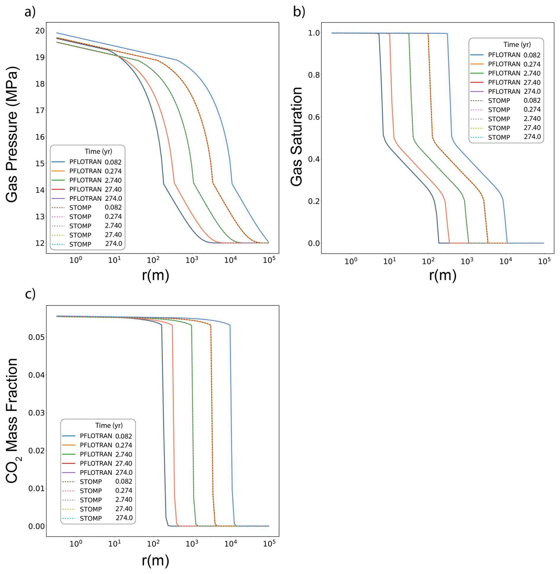
Figure 2Radial Flow of Supercritical CO2 without salt: (a) Gas Pressure, (b) Gas Saturation, (c) CO2 Aqueous Dissolved Mass Fraction.
3.1.2 With Salinity
In this variant of the Radial Flow of Supercritical CO2 benchmark problem, CO2 is injected into a brine aquifer characterized by an initial constant dissolved salt mass fraction. Both PFLOTRAN and STOMP-CO2 simulators were run with the same model setup; plots of a select set of output variables vs radial distance from the wellbore are shown below. These output variables include gas pressure, gas saturation, dissolved CO2 mass fraction, and salt precipitate saturation (Fig. 3). For this problem, PFLOTRAN and STOMP-CO2 results are very close for all variables, indicating very strong agreement between the two simulators and verifying the implementation in PFLOTRAN. PFLOTRAN and STOMP-CO2 differ slightly in their reporting of precipitate saturation very close to the wellbore; here, both simulators show a small amount of numerical oscillation. Under strict time step control to small time steps, this numerical oscillation can be eliminated.
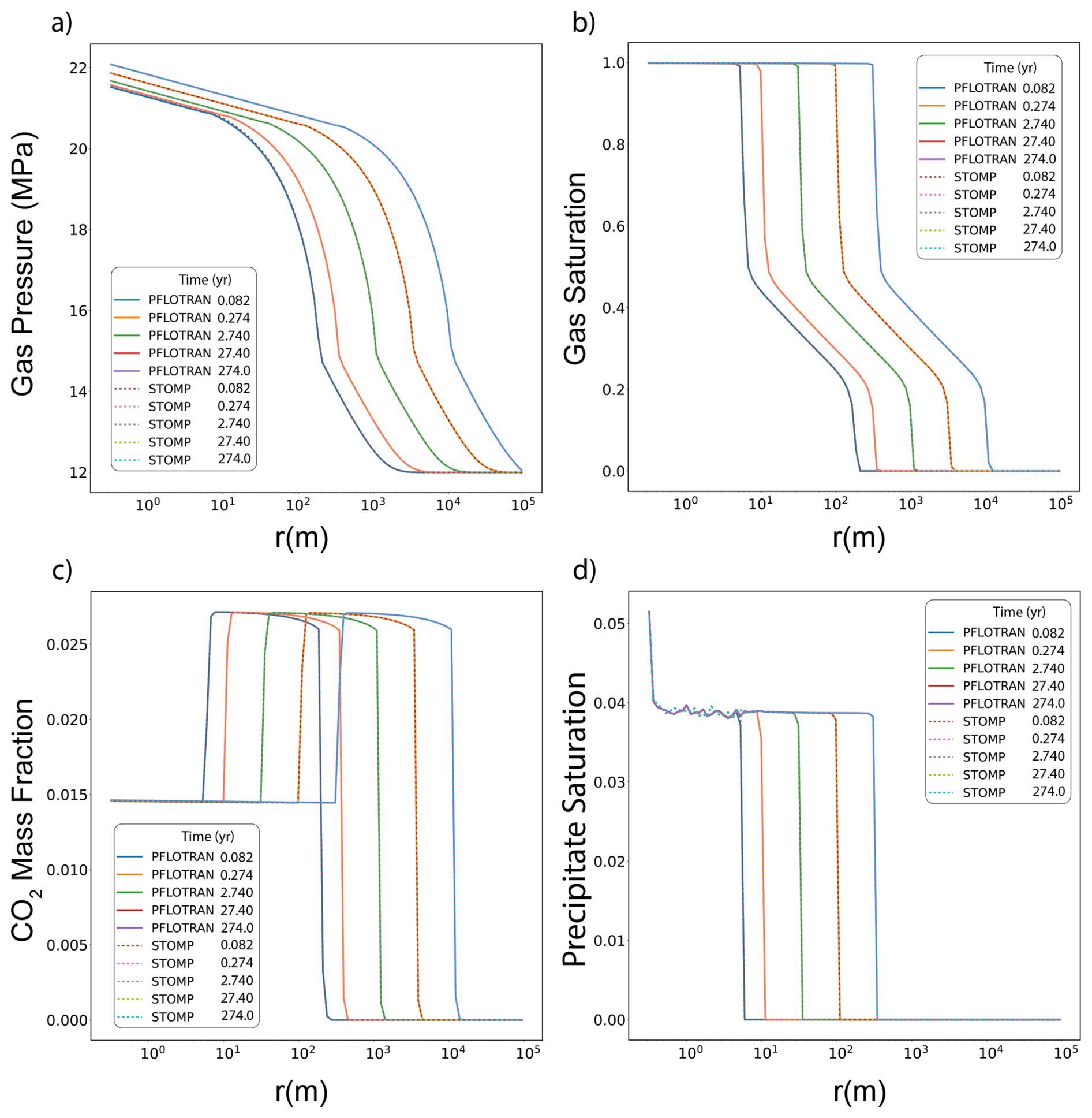
Figure 3Radial Flow of Supercritical CO2 with salt: (a) Gas Pressure, (b) Gas Saturation, (c) CO2 Aqueous Dissolved Mass Fraction, (d) Salt Precipitate Saturation.
This benchmark demonstrates the ability of PFLOTRAN's SCO2 Mode to solve coupled, isothermal CO2 and brine flow in a radial domain with and without fully implicit salinity coupling. These results are consistent with those produced by STOMP-CO2 for the same set of tests. Since this is a 1D radial model, buoyancy effects are not evaluated by this test. The following benchmark evaluates PFLOTRAN's ability to model CO2 buoyancy.
3.2 Discharge of CO2 Along a Fault
This benchmark builds on the previous test by adding gravity effects. Here, simulators are challenged to model buoyant vertical flow rather than simply radial flow. This is important for evaluating vertical migration CO2 and the sealing capacity of a caprock. Furthermore, gravity effects will be present in the remainder of the test simulations presented in this work.
This benchmark problem is equivalent to STOMP-CO2 Short Course Example Problem CO2-2. Like the Radial Flow of Supercritical CO2 benchmark problem, this problem was also introduced as part of the GeoSeq Project (Pruess et al., 2002). Here, a 1D vertical Cartesian domain is initialized to hydrostatic conditions with pure water (no dissolved salt). This vertical model is meant to emulate loss of stored CO2 into a freshwater aquifer along a leaky fault. This problem tests the ability of simulators to model displacement of water by buoyant CO2 migration, dissolution of CO2 at the gas-water interface, hydrostatic water pressure and a Dirichlet top water pressure boundary, and a bottom gas pressure boundary that drives CO2 flow into the domain.
Pressure at the top of the domain (500 m) is set to 10 MPa, and temperature everywhere is set to 45 °C. The model is isothermal. The model is run in two stages: first, an equilibration step obtains an initial pressure distribution (though the keyword HYDROSTATIC in PFLOTRAN can also be used to apply a hydrostatic pressure distribution); second, the model is restarted with a Dirichlet gas phase boundary condition imposed on the bottom boundary and characterized by a gas pressure of 24 MPa. Table 3 summarizes key properties of the model.
Both PFLOTRAN and STOMP-CO2 simulators were run with the same model setup; plots of a select set of output variables versus height of the column are shown below. These output variables include gas pressure, gas saturation, aqueous dissolved CO2 mass fraction, and mass fraction of CO2 in the gas phase (Fig. 4). For this problem, PFLOTRAN and STOMP-CO2 results are nearly indistinguishable, indicating very strong agreement between the two simulators and verifying the implementation in PFLOTRAN.
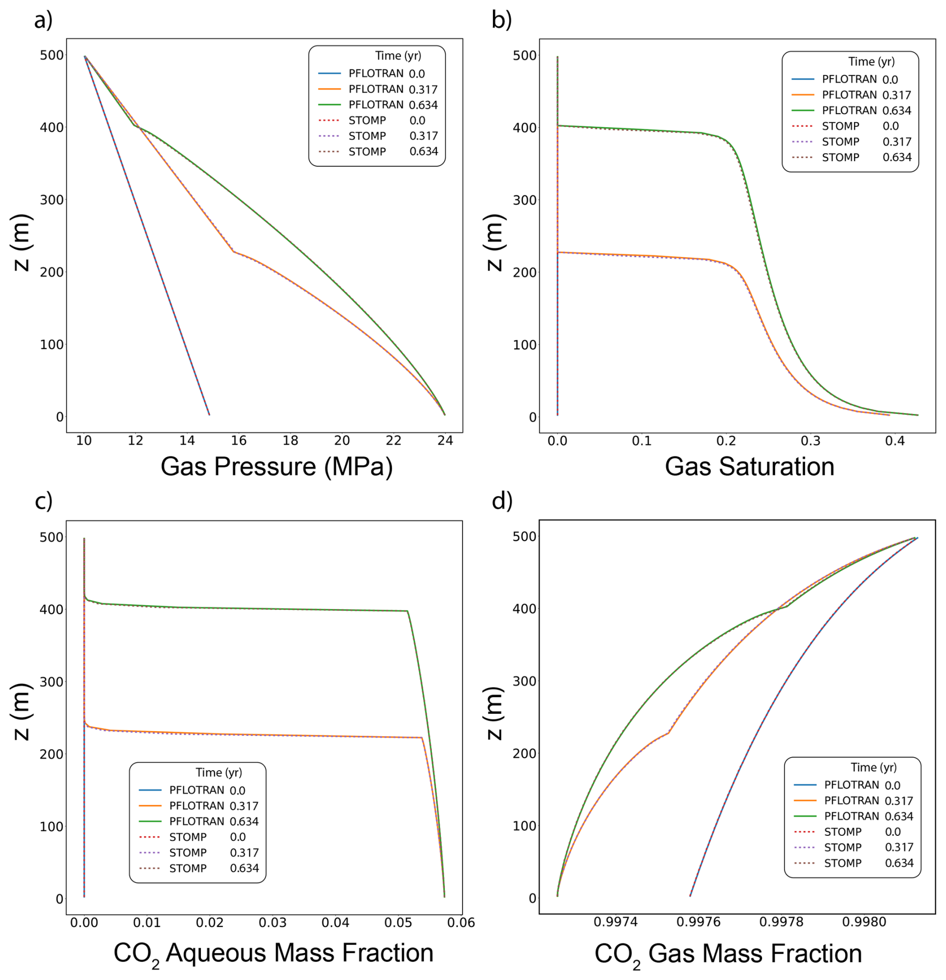
Figure 4CO2 Discharge Along a Fault: (a) Gas Pressure, (b) Gas Saturation, (c) CO2 Aqueous Dissolved Mass Fraction, and (d) Free-phase CO2 Gas Mass Fraction.
This benchmark demonstrates the ability of PFLOTRAN's SCO2 Mode to solve buoyant flow of CO2 in a 1D Cartesian domain. These results are consistent with those produced by STOMP-CO2 for the same test.
Table 42D CO2 Injection into a Layered Formation: Model Properties.
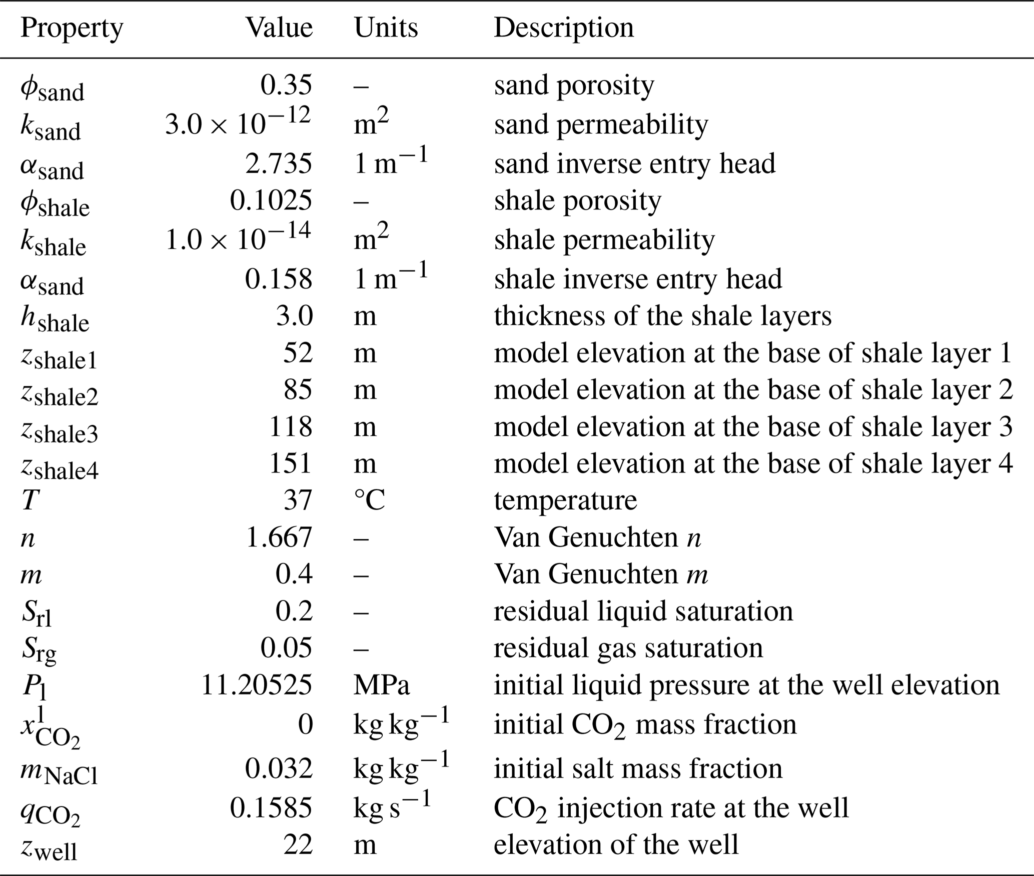
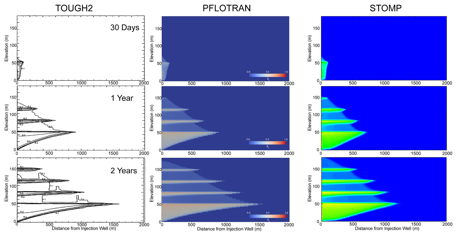
Figure 5TOUGH2, PFLOTRAN, and STOMP-CO2 Comparison. TOUGH2 results adapted from (Pruess et al., 2002), and STOMP-CO2 results adapted from STOMP-CO2 Short Course Problem CO2-3 (White, 2023).
3.3 CO2 Injection into a 2D Layered Formation
This benchmark is designed to test the ability of simulators to model CO2 migration in 2D both vertically and horizontally in the presence of lithologic heterogeneity. This problem presents a more realistic scenario where injected CO2 becomes trapped beneath low permeability sealing layers.
This benchmark problem is equivalent to STOMP-CO2 Short Course Example Problem CO2-3. This problem was originally developed for the GeoSeq project (Pruess et al., 2002). Here, a 2D Cartesian layered model was designed to be representative of the Sleipner Vest field in the Norwegian North Sea. The problem contains alternating sand and shale sequences in a marine environment (i.e., saline pore water).
The problem is isothermal at 37 °C, and a source term injects scCO2 into the bottom left corner of a sandy reservoir unit beneath the deepest shale layer. The model is initialized to hydrostatic liquid pressure with a pressure of 11 MPa at the elevation of the injection well, 22 m from the bottom of the domain. No flow boundary conditions are applied on the left as a symmetry boundary, top as an impermeable shale seal, and bottom as another impermeable seal. The right boundary is a Dirichlet boundary at hydrostatic conditions. The domain spans 6 km horizontally and 184 m vertically, with a series of four 3 m thick horizontal shale units at different depths and spanning the entire length of the domain.
The sand layers and shale layers are characterized by different lithologic properties, adding heterogeneity to the model. They have different permeabilities, porosities, and capillary entry pressures. ScCO2 is injected for a period of 2 years at a single well location in the model and at a constant rate of 0.1585 kg s−1. Table 4 summarizes key properties of the model.
Simulation results are shown for PFLOTRAN, STOMP-CO2, and published results using TOUGH2 (Pruess et al., 2002) at 30 d, 1 year, and 2 years (Fig. 5). ScCO2 initially migrates buoyantly upward from the injection site through the sand reservoir until it reaches a lower permeability shale layer, where it begins to spread laterally. Over time, due to capillary entry pressure and permeability contrasts, free-phase CO2 accumulates at the interface between layers in the model. Overall, there is good agreement between PFLOTRAN, STOMP-CO2, and TOUGH2, verifying the implementation in PFLOTRAN (Fig. 5). PFLOTRAN exhibits slightly more curvature in the the free-phase CO2 plume than STOMP-CO2, which is more plug-like. The PFLOTRAN model more closely matches TOUGH2 in this regard.
Table 52D Cylindrical Injection: Model Properties.
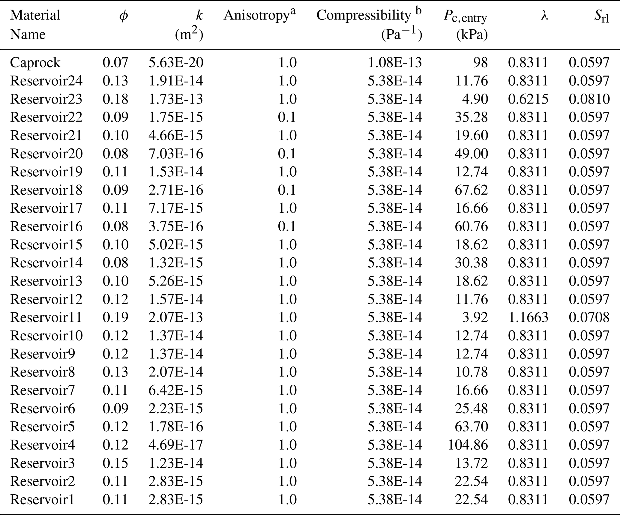
a Vertical: Horizontal permeability anisotropy ratio. b Linear porosity compressibility.
This benchmark demonstrates the ability of PFLOTRAN's SCO2 Mode to model 2D migration of CO2 in a heterogeneous domain. PFLOTRAN results are in good agreement with both TOUGH2 and STOMP-CO2 simulators run on the same test problem. The PFLOTRAN results generally fall between the results of TOUGH2 and STOMP-CO2. These small differences could be attributable to differences in numerical diffusion resulting from different time stepping algorithms or subtle differences in numerical implementation between codes.
3.4 2D Cylindrical Injection with a Fully Coupled Well Model
In addition to the coupled processes verified by the first three benchmark test cases, this benchmark also tests the ability of SCO2 Mode to model fully coupled wells with pressure control, unsaturated capillary pressure curve extensions, trapped gas hysteresis, permeability anisotropy, fixed temperature gradient, and gravity in a 2D cylindrical domain. These are all potentially important features for understanding the fate of a subsurface CO2 injection.
This benchmark problem is equivalent to STOMP-CO2 Short Course Example Problem CO2-4. Here, a well model is used to inject scCO2 into a layered brine reservoir with heterogeneous permeability and capillary entry pressure. The model consists of 1 caprock layer at the top of the domain and 24 reservoir layers of varying thickness (Table 5). The original model, developed for STOMP-CO2, uses a mixture of Imperial and SI units; here, all units were converted to SI units. Maximum trapped gas saturation for trapped gas hysteresis calculations is set at 0.2 for all layers in the domain. The model is initialized to hydrostatic pressure and a geothermal gradient of 20 °C km−1, with a pressure of 12.34 MPa and temperature of 43.75 °C at an elevation of −1040 m. Initial salt mass fraction in the brine is set to 0.0475 kg kg−1. The fracture pressure of the reservoir is set to 16.4 MPa; if pressures in the wellbore exceed this pressure, the well becomes rate-controlled. The wellbore diameter is set to 0.2286 m with no well skin. The well injects CO2 at a constant rate of 1.0 MMT yr−1 for the first 2 years. Then the injection well switches off and the model continues to run for a total simulation time of 10 years. The cylindrical grid increases in the radial direction from a cell radius of 5.2 m in the innermost cell to 551.2 m at the far edge for a total of 20 cells in the radial direction. In the vertical dimension, cell thickness varies from 1.2 to 24.99 m in thickness over a total of 25 cells.
PFLOTRAN and STOMP-CO2 results are nearly identical (Fig. 6). They show slight differences in the radial extent of the CO2 plume in a few of the cells at the outer edge of the plume. Other than this, the magnitude and distribution of free phase CO2 saturation match between the two simulators, verifying the implementation of the well model with pressure control, trapped gas hysteresis, and capillary pressure extensions in PFLOTRAN.
This benchmark demonstrates the ability of PFLOTRAN's SCO2 Mode to model CO2 injection into a 2D cylindrical domain using a fully coupled hydrostatic well model. PFLOTRAN results are in good agreement with those produced by STOMP-CO2 for the same test; simulators show some differences in gas saturation at the outer edges of the CO2 plume. These differences could be attributable to differences in numerical diffusion resulting from different time stepping algorithms or subtle differences in numerical implementation between codes.
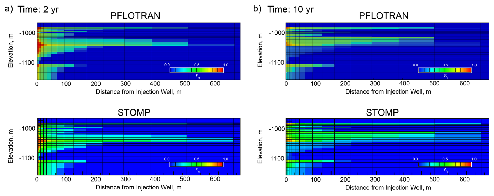
3.5 Mineral Trapping in Basalts
Recently, reactive basalt and mafic/ultramafic formations have been targeted as CO2 storage sites due to their unique ability to rapidly mineralize CO2 (Matter et al., 2011; McGrail et al., 2017; Raza et al., 2022). This benchmark tests the ability of simulators to couple multiphase CO2-brine flow with reactivity to store CO2 in mineral form.
This benchmark problem is equivalent to STOMP-CO2 Short Course Example Problem CO2-6. This problem simulates injection of CO2 into a reactive basalt reservoir by coupling SCO2 Mode with the GIRT reactive transport mode in PFLOTRAN. The physical and geochemical properties in this scenario are designed to emulate those of the Grande Ronde continental flood basalts of the Columbia Plateau province in southeastern Washington state. In this system, high permeability basalt flow tops have been targeted as potential reactive reservoirs for CO2 storage; these flow tops are sandwiched between low permeability flow interiors which serve as confining layers and create a stacked reservoir. The Wallula Basalt Pilot Project, which injected roughly 1000 MT of CO2 into one such reservoir system in 2013, demonstrated the ability of highly reactive basalts to rapidly mineralize CO2 in the subsurface (McGrail et al., 2017).
Here, CO2 is injected into a single flow top reservoir in a 2D cylindrical domain. No flow boundaries are applied at the top and bottom to simulate a flow top confined between two impermeable flow interiors. The model is initialized with a hydrostatic brine pressure distribution and temperature following a geothermal gradient of 26.8 °C km−1, with a brine pressure of 10 MPa and temperature of 39.83 °C at a datum of −1087.53 m elevation. Salt mass fraction is initially set to 0.01 kg kg−1 everywhere. CO2 is injected along the entire span of the reservoir unit at r=0 m at a total mass injection rate of 0.827 kg s−1 for a total of 1000 Mt of CO2 injected after 14 d. At the end of 14 d, the CO2 source is shut off and the model is run to a total simulation time of 10 years.
PFLOTRAN and STOMP-CO2 results show good agreement. The pH distribution in the reservoir is controlled by the movement of dissolved CO2 through the system (Fig. 7); pH profiles after 10 years show similar distributions and magnitudes between STOMP-CO2 and PFLOTRAN. STOMP-CO2 shows a bit more spread in the pH plume than PFLOTRAN, and the pH decrease reaches slightly further in the radial direction. This is consistent with results obtained from previous benchmarks, but it also is likely affected by stronger mineralization reported by PFLOTRAN (Fig. 8). The differences could be due to several factors: first, there are likely differences in PFLOTRAN's GIRT mode implementation of the reactive transport equations as compared to STOMP. Second, just like in previous benchmarks, STOMP-CO2 used a combination of imperial, field, and SI units. These values (depths, pressures, temperatures, etc) were converted to SI units for use in PFLOTRAN. Finally, STOMP-CO2 allows the user to specify a hydrostatic gradient to initialize the model, while PFLOTRAN computes hydrostatic pressure internally relative to a datum. The pressure solution will evolve in response to boundary conditions as well as the evolution of CO2 and salt mass distributions; final pressures could be sensitive to initialization and the far-field boundary pressure.
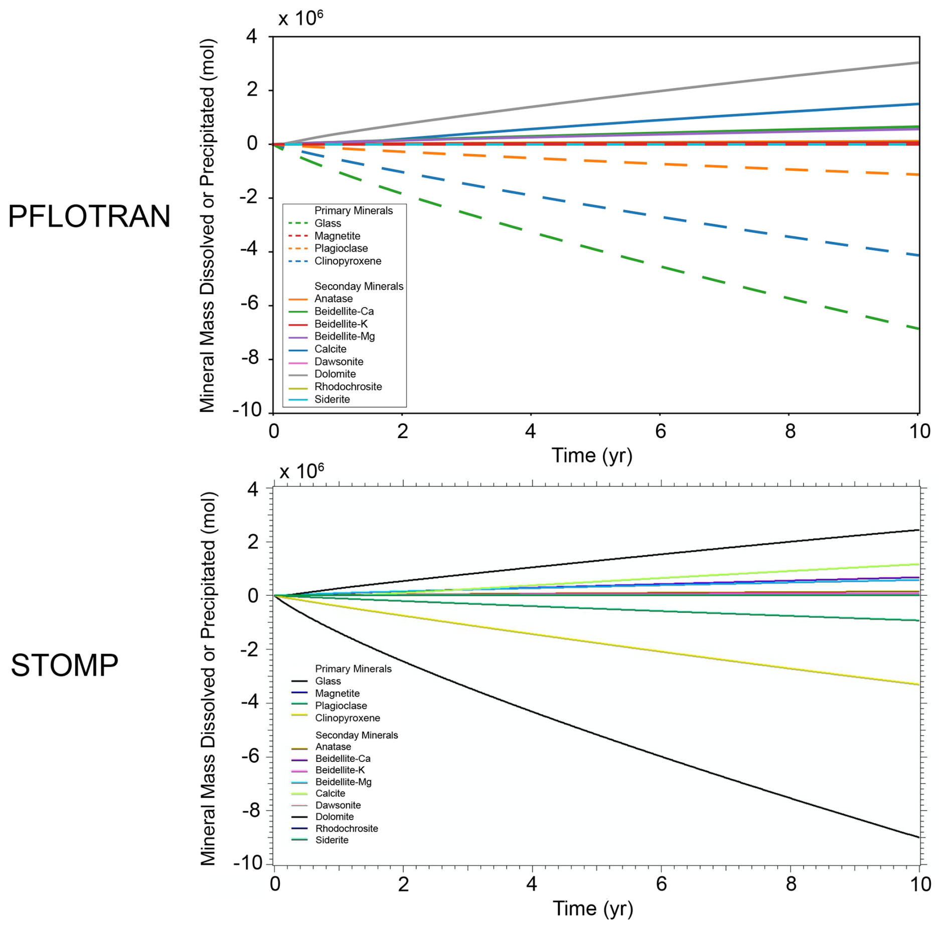
There is good agreement between PFLOTRAN and STOMP-CO2 with respect to the evolution of primary and secondary mineralogy in the system (Fig. 8). Both simulations agree in terms of order of magnitude of dissolution and precipitation, as well as mineral order of importance. For both models, glass was the most dominant primary mineral to dissolve, followed by clinopyroxene, plagioclase, and magnetite. Likewise, dolomite was the most dominant secondary carbonate mineral formed, followed by calcite, beidellite-Ca, beidellite-Mg, and then the others. In addition to the differences noted above and in previous benchmark tests, differences in mineral volumes could also have to do with kinetic reaction rates in STOMP-CO2 being supplied at different reference temperatures; reaction rates were adjusted to a common reference temperature of 25 °C for PFLOTRAN.
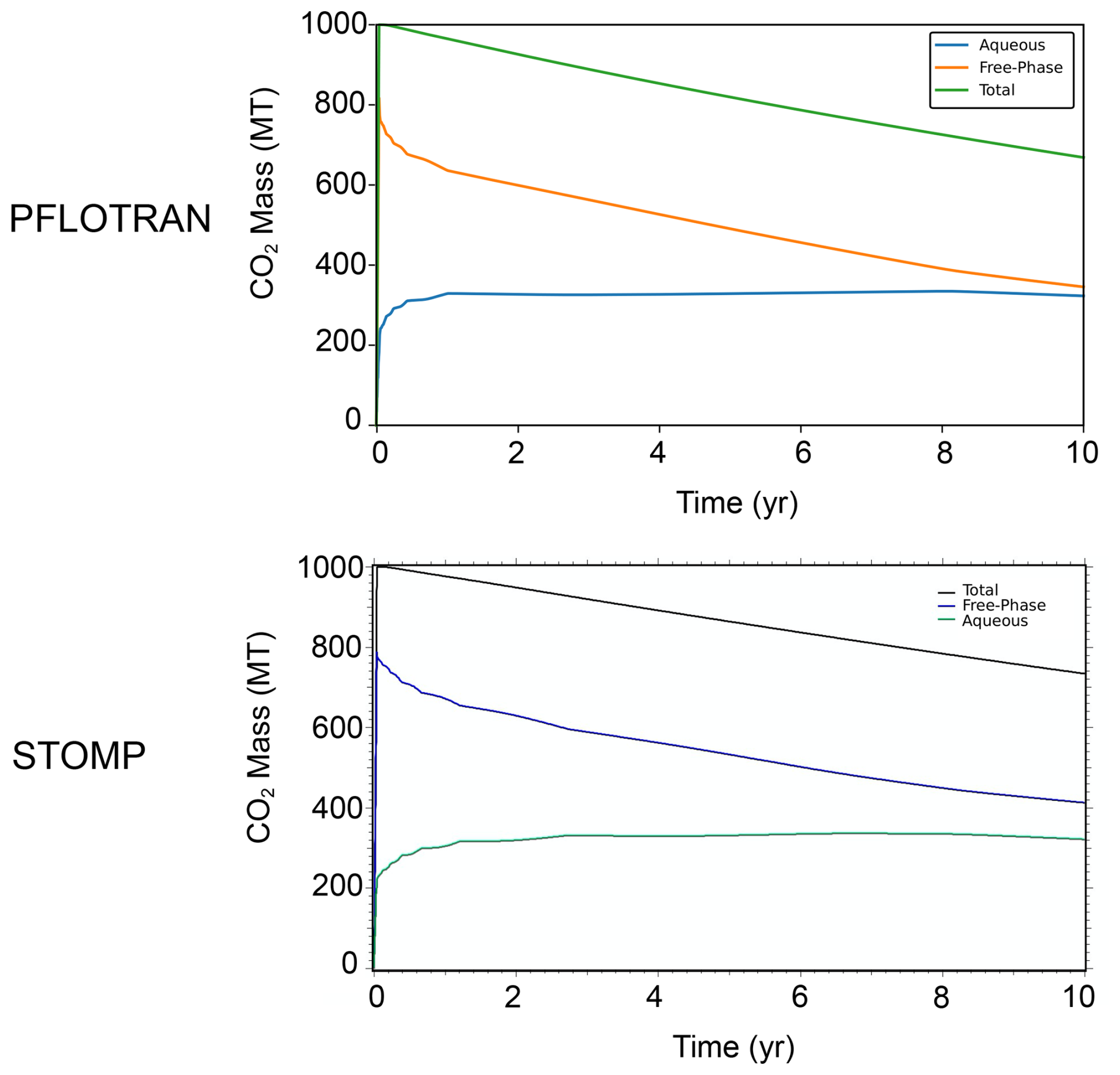
The global CO2 mass balance tells a similar story (Fig. 9). Both PFLOTRAN and STOMP-CO2 report roughly the same total amount of dissolved CO2 in the whole model, but they differ slightly in the amount of free-phase CO2. This is likely attributable to PFLOTRAN reporting slightly higher amounts of carbonate mineralization in comparison to STOMP-CO2, particularly dolomite mineralization. Mineralization could be retarding the movement of CO2 through the system, which is also expressed in the pH plume. Total free CO2 mass (the sum of dissolved and free gas mass) is consistent between both simulators at the end of the injection period, and by 10 years PFLOTRAN reports slightly lower total free CO2 mass; the difference is attributable to differences in total mineralization (negligible amounts of CO2 leave the far-field boundary). Overall, good agreement between the two simulators verifies the implementation of CO2 flow coupled to mineral dissolution/precipitation and aqueous reaction networks in PFLOTRAN.
This benchmark demonstrates the ability of PFLOTRAN's SCO2 Mode to model coupled CO2-brine flow and CO2 mineralization in reactive host rocks in a 2D cylindrical domain. PFLOTRAN results are generally in good agreement with those produced by STOMP-CO2 for the same test. Simulators show some differences in overall CO2 mineralization; these differences are likely attributable to differences in the implementation of reactive transport between the simulators.
Injecting CO2 into subsurface reservoirs naturally acidifies the formation water, as the benchmark tests presented here have shown. In highly reactive basalt rocks, this can dissolve a host rock rich in cations that then react with dissolved CO2 to form secondary carbonate minerals. However, in addition to promoting carbonate reactions in basalts, acidic solutions can also promote leaching of critical minerals from ore deposits; in situ leach mining is an established technique to recover metals from ores in situ such as uranium, gold, copper, and others (Bartlett, 2013). Here we demonstrate how CO2 could be used to promote leaching and in situ production of a copper ore deposit. This process has the dual benefit of storing CO2 and producing valuable critical minerals.
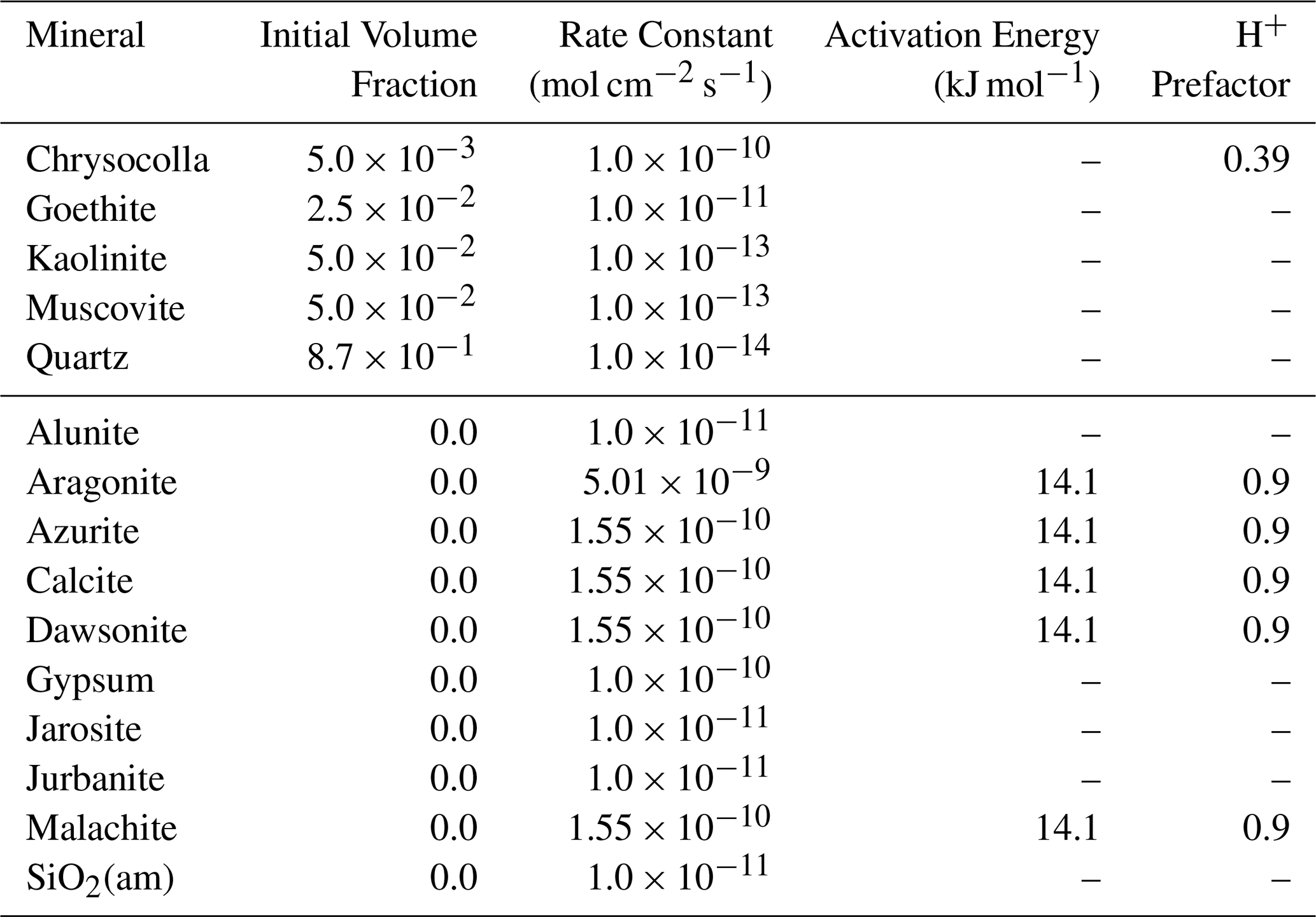
In this example, a horizontal well is drilled through a hypothetical copper ore deposit. The domain measures 750 m in both lateral directions and 120 m vertically. The ore itself spans the domain laterally and 80 m vertically. It is situated between two impermeable sealing layers. The injection well extends down to the bottom of the ore deposit, where it then kicks off to horizontal for 400 m. The last 300 m of the lateral length of the well are screened; the rest of the well is cased. The initial mineral composition of the deposit is based on Hammond et al. (2014) and is shown in Table 6. The reservoir conditions are such that CO2 is a supercritical fluid: formation temperature is 40 °C at the top of the domain and increases by 28 °C km−1 with depth. Liquid pressure at the top of the domain is 8.3 MPa, and the formation brine has an initial salt mass fraction of 0.01 kg kg−1. The well injects CO2 and extracts formation fluids over three cycles for a total copper production period of 20 years. The well first injects 1 kg s−1 of CO2 for one year, then shuts off for 3 months to allow CO2 to migrate and react with water to dissolve the rock minerals; the well then extracts formation fluids for one year at a rate of 1 kg s−1. The process is repeated twice more, and then the production rate is held constant until year 20.
After 5.5 years, three cycles of CO2 injections have injected a total of 9.46 × 10⁵ MT of CO2 through the well. A buoyant free-phase CO2 plume migrates upward through the reservoir above the well; since the CO2 is also dissolved in the pore water, the associated change in pH of the pore water extends beyond the free-phase CO2 plume, which results in a zone of enhanced copper dissolution (Fig. 10). In this model, the minimum pH induced by CO2 injection is 4.3. The original formulation of the copper leaching problem from Hammond et al. (2014) injects an aqueous solution with a strong acid of pH 1 into an ore deposit to induce copper leaching. For comparison, we modified our example problem to inject an aqueous solution with the acid used in Hammond et al. (2014) instead of CO2. As expected, a very strong acid initially results in greater amounts of copper extracted from the deposit (Fig. 11). But, interestingly, at later time copper extraction rates decay slower with CO2 injection than with acid injection. This could be due to the differences in mobility between CO2 and water and suggests that an optimal CO2 injection strategy could be achieved that balances the timing of injection and production with the rates of free-phase CO2 migration, copper leaching, and copper carbonate mineralization.
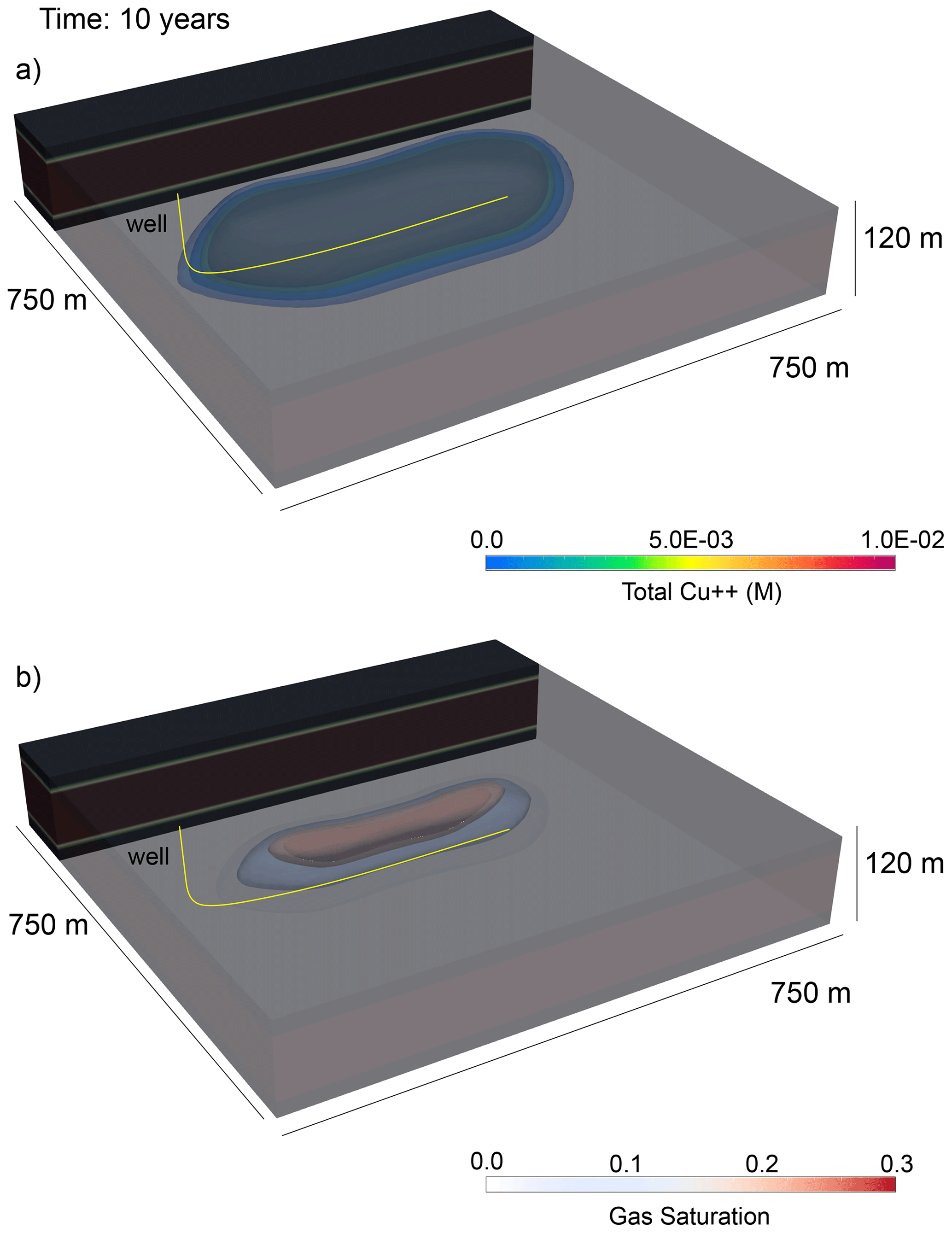
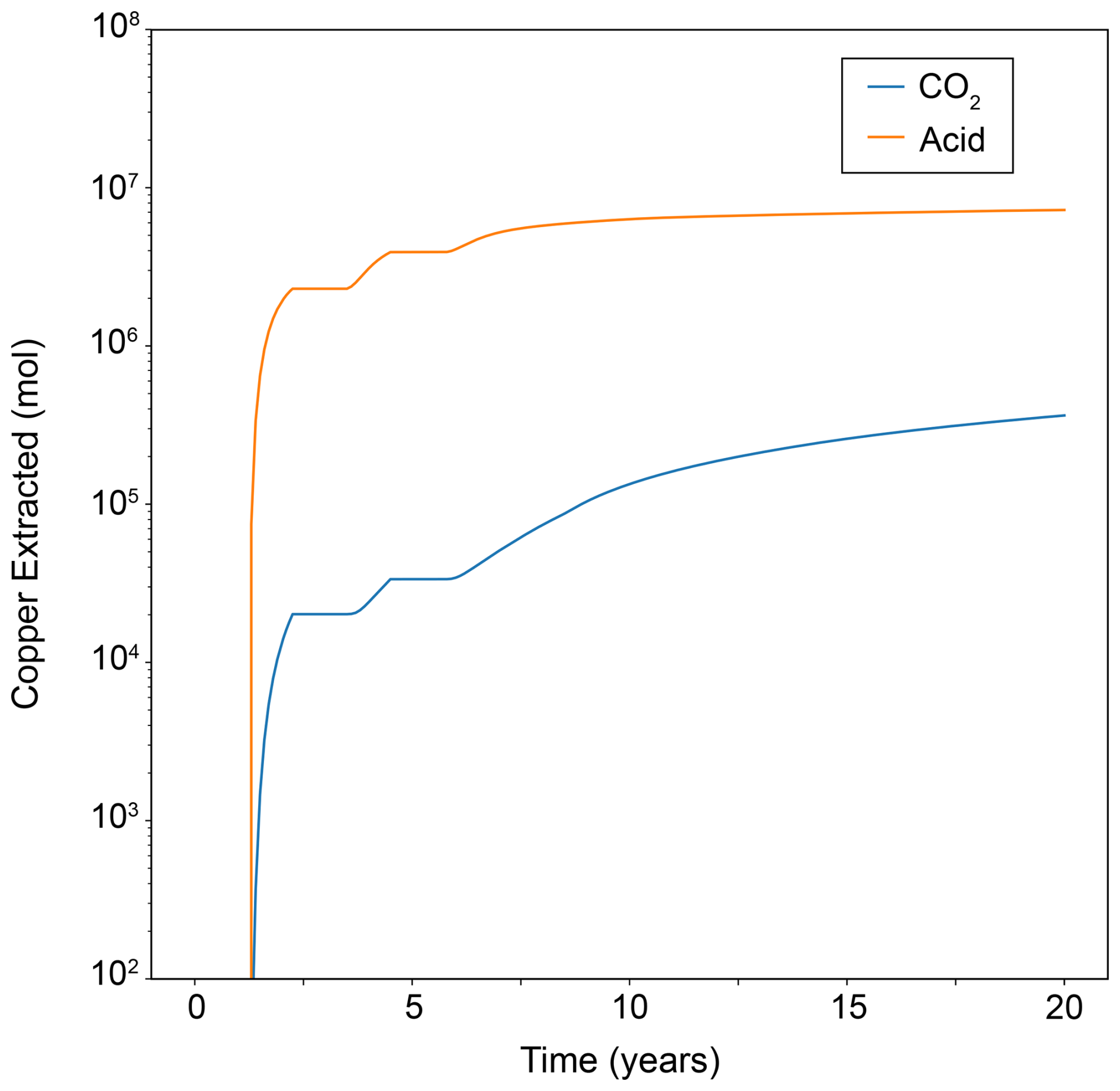
Figure 11Total copper mass extracted from the well over 10 years, comparing CO2 as the acidification agent to a strong acid (pH = 1).
In addition to differences in system pH between a CO2 injection and an acid injection, CO2 can also react with copper cations in solution to form copper carbonates. In this model, the dominant copper carbonate mineral that forms is malachite, while the primary mineral that dissolves to release copper is chrysocolla (Fig. 12). Interestingly, silica formation accounts for a significant fraction of the total mass of minerals formed, indicating that silica formation rates could be affecting overall mineral dissolution/precipitation and thus total copper extraction potential.
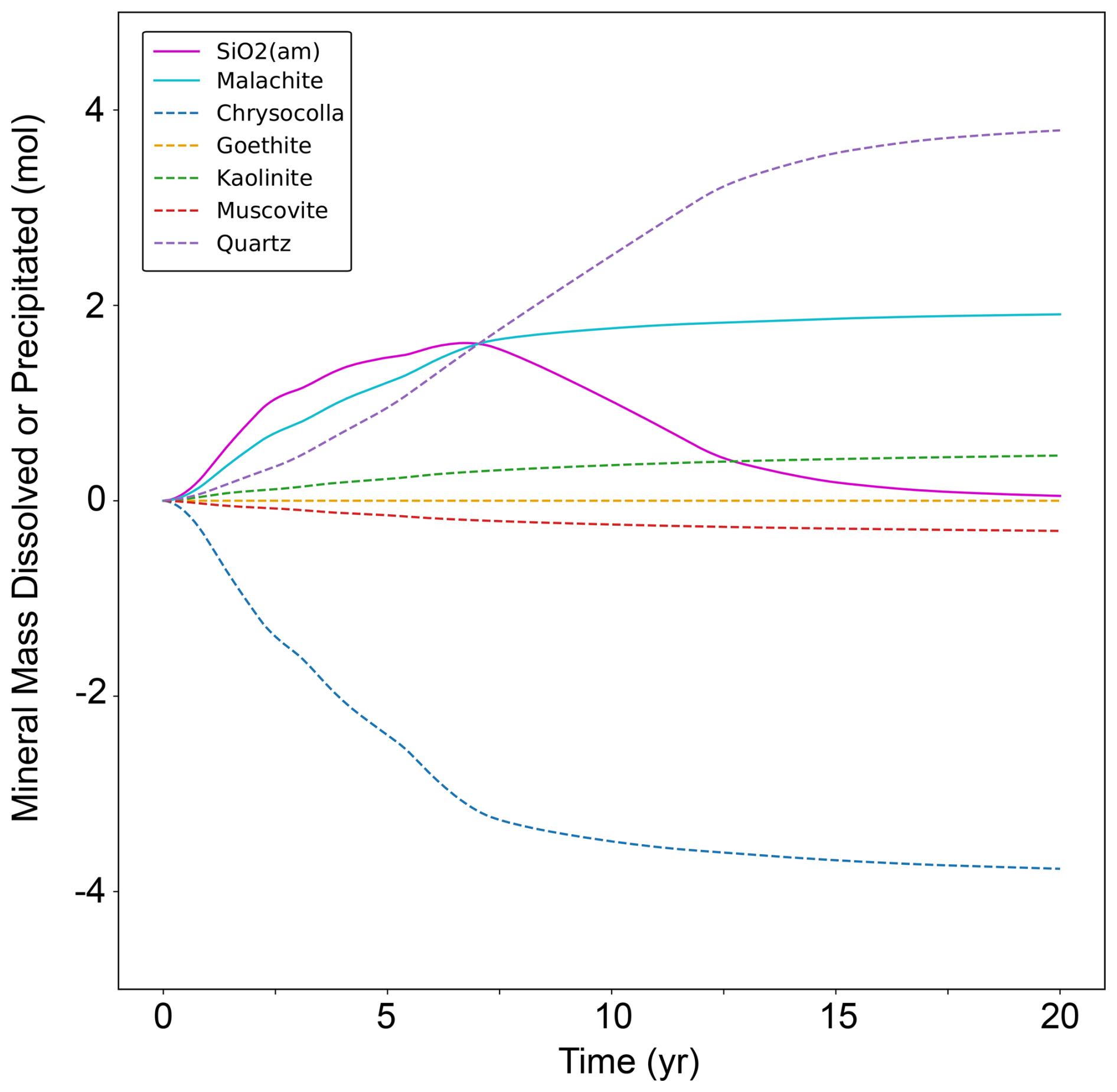
Figure 12Total mineral mass precipitated (positive) or dissolved (negative) as the result of CO2 injection. Dashed lines indicate primary minerals.
Recent developments in the open source multiphase flow and reactive transport simulator PFLOTRAN now allow for modeling the flow of scCO2 and brine with optional fully implicit coupling to a hydrostatic well model, fully implicit thermal coupling, and sequential coupling to PFLOTRAN's well-established reactive transport capabilities. Many new features are now available, including flexible well trajectories, capillary pressure function extensions below residual saturation, and scanning path hysteresis for gas trapping. These new features are verified against the STOMP-CO2 simulator for five benchmark test cases, which show excellent agreement between the two simulators. Finally, a new example problem involving critical mineral extraction is presented, demonstrating how CO2 can be used as a working fluid for promoting copper leaching from an ore deposit. Critical mineral extraction using CO2 as the working fluid would take advantage of CO2-induced acidification to leach copper into the pore water, but the process should be optimized to avoid significant mineralization of secondary copper carbonate minerals. This example demonstrates how CO2 could be used instead of strong acids to extract critical minerals using a potentially more environmentally friendly working fluid while simultaneously storing CO2.
The results of this study establish confidence in the ability of PFLOTRAN's SCO2 mode to model coupled flow of CO2 and brine in the subsurface. This will allow users to leverage the scalability and transparency of PFLOTRAN to model large-scale CO2 storage in conventional reservoirs. Coupling SCO2 mode with PFLOTRAN's well-established reactive transport libraries has also unlocked new opportunities for modeling mineral dissolution and precipitation in reactive host rocks subjected to CO2 injection. In the future, this capability can be used to model large-scale CO2 storage, CO2 mineralization, and critical mineral extraction processes with confidence in both the multiphase flow and the reactive transport components of these models.
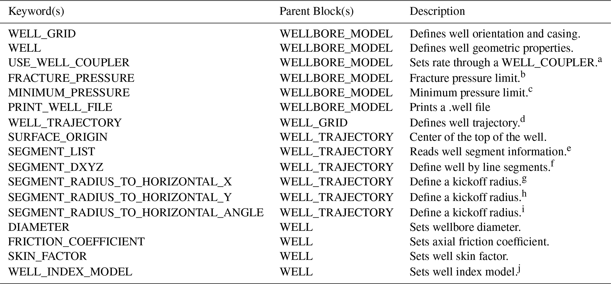
The following section describes new input parameters specific to SCO2 Mode, the well model, and coupling with reactive transport. All other base PFLOTRAN functionality (e.g., gridding, material property definition, output options, dataset I/O, etc) can be used with SCO2 Mode just like all other flow modes (see the PFLOTRAN Documentation, https://documentation.pflotran.org, last access: 18 December 2025, for more details).
Running models with SCO2 Mode requires invoking the flow mode through the input deck and then choosing from a variety of input options specific to SCO2 Mode. Several new options have been added to the input deck that allow the user to choose the functionality they desire and parameterize accordingly. The following sections provide the user with a description of new input options, associated keywords, and snapshots of input decks providing context on where those keywords are used.
A1 New Inputs
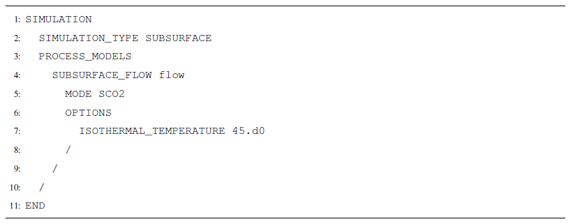
The two highest-level input blocks required to run a subsurface model with SCO2 Mode are the SIMULATION and SUBSURFACE blocks. In the SIMULATION block, the user chooses which process models they would like to simulate. Those can include any combination of flow modes, transport modes, geomechanics, well models, and more. PFLOTRAN will couple these processes together according to their default coupling schemes and provide coupling options where available. To select SCO2 Mode, the user would invoke MODE SCO2 under SUBSURFACE_FLOW within the PROCESS_MODELS sub-block of SIMULATION.
Additionally, an OPTIONS block within SUBSURFACE_FLOW can be used to define certain refinements to the process model. Most notably, this is where the user would decide whether to run an isothermal simulation or a non-isothermal simulation. To run isothermal, the user has two options: first, ISOTHERMAL_TEMPERATURE <temperature value> sets a single constant temperature equal to <temperature value> throughout the entire model domain. Second, the user could invoke FIXED_TEMPERATURE_GRADIENT to specify initial temperature conditions in the model and keep those temperatures fixed over time. Use of the FIXED_TEMPERATURE_GRADIENT keyword requires including thermal state variables in the FLOW_CONDITIONs and then setting cell temperatures through an INITIAL_CONDITION.
Other options in the OPTIONS block include:
-
UPDATE_SURFACE_TENSION scales the CO2-brine-rock interfacial tension as a function of temperature and brine saturation, which in turn affects capillary pressure. Otherwise, no interfacial tension scaling is used.
-
MIXTURE_DENSITY provides options for computing CO2-brine mixture density.
-
UPWIND_VISCOSITY fully upwinds the viscosity for use in flux calculations.
-
PHASE_PARTITIONING can select the CO2-brine equilibrium phase partitioning calculation method.
-
NO_H2O_SOURCE_UPDATE_FROM_TRANS turns off water source/sink due to mineralization reactions if reactive transport is being used
Another option in the PROCESS_MODELS block is to invoke the WELL_MODEL. The WELL_MODEL then expects a TYPE. Currently, TYPE HYDROSTATIC is supported by SCO2 Mode, and the well model coupling strategy is fully implicit. The PROCESS_MODELS block is also where a user would request the SUBSURFACE_TRANSPORT for coupling flow, a well model, and/or reactive geochemical transport. A list of new keywords can be found in Table A1.
Table A1Input Deck Keywords.
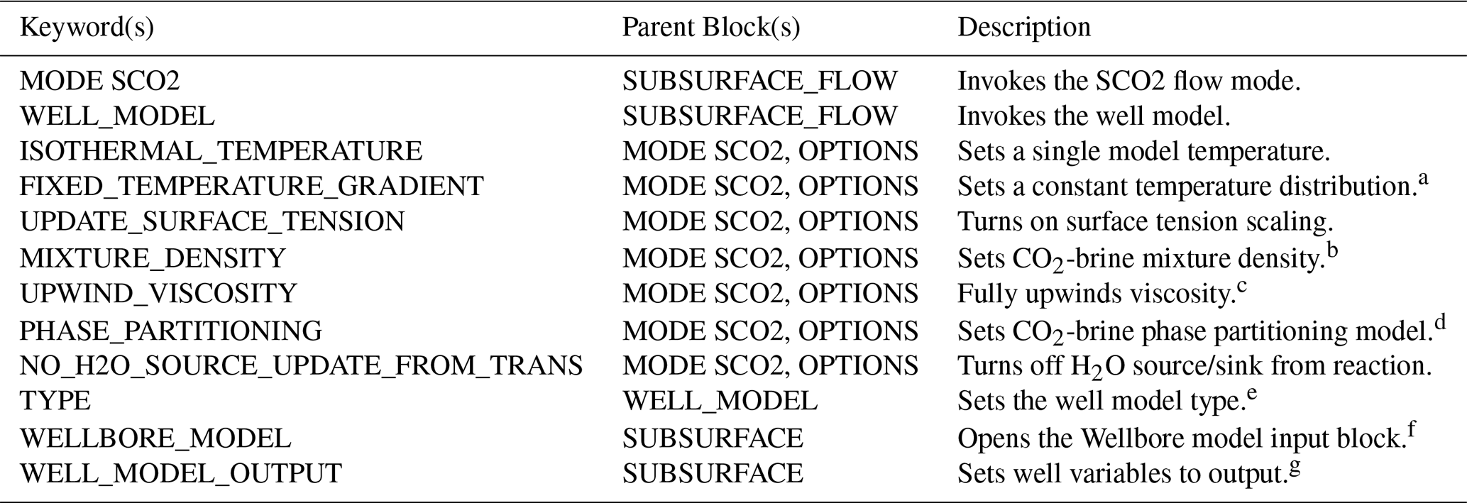
a Temperature distribution is read in through an INITIAL_CONDITION the same way as a thermal model, and it is held constant throughout the simulation. b Options: GARCIA (default is Alendal and Drange, 2001). c Default is a harmonic average. d Options: SPYCHER_SIMPLE. Default is Spycher and Pruess (2010). e Options: HYDROSTATIC is the only supported option with SCO2 Mode. f This is where the user defines all well properties including well trajectory, geometry, flow rate, and well index relationship. Use multiple WELLBORE_MODEL blocks to define multiple wells. g Options: WELL_LIQ_PRESSURE, WELL_GAS_PRESSURE, WELL_LIQ_Q, WELL_GAS_Q.
Within the SUBSURFACE block, several new options have been added to simulate injection and production wells. The WELLBORE_MODEL block is used to begin defining the properties of a well. Multiple WELLBORE_MODEL blocks can be used to define multiple wells, each with different properties. Each WELLBORE_MODEL block requires a name (e.g., WELLBORE_MODEL well-1, WELLBORE_MODEL well-2). Within a WELLBORE_MODEL block, several sub-blocks are used to build different parts of the well and apply specific constraints. The first sub-block is the WELL_GRID block, which is used to define the orientation and trajectory of a particular well. The WELL block defines properties of the wellbore itself, like diameter and skin factor. Pressure limitations can be imposed by the FRACTURE_PRESSURE and MINIMUM_PRESSURE keywords. A list of keywords can be found in Table A3, and more information on well model construction can be found in Sect. A3.
A1.1 New Characteristic Curve Options
A new, head-based Van Genuchten characteristic curve option is now available. This model takes the following form:
where hgl is the gas-liquid capillary head in meters, α is the inverse of the capillary entry head in m−1, βgl is the interfacial tension scaling factor, and is a liquid reference density, which by default is set to 998.32 kg m−3.
This new capillary head-based saturation function is invoked with keyword VG_STOMP (Table A2). Both the Van Genuchten capillary head function and the default Brooks-Corey capillary pressure function can now be optionally extended into the region below residual liquid saturation by using the UNSATURATED_EXTENSION keyword. Both functions are also now compatible with the scanning path hysteresis model for gas trapping.
Table A2Characteristic Curve Keywords.
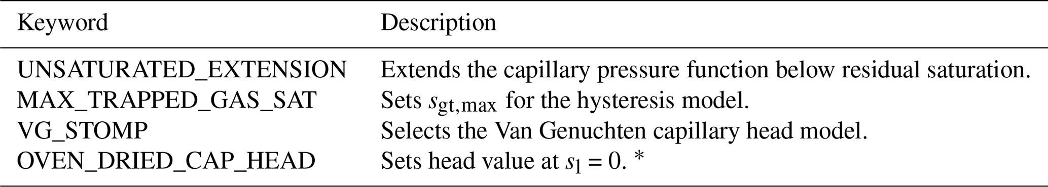
* Applies to Van Genuchten capillary head function only, used when extending the capillary head curve below residual saturation.
Table A3Well Model Keywords.
a A WELL_COUPLER block links FLOW_CONDITIONs and TRANSPORT_CONDITIONs to WELLs in the same manner as INITIAL_CONDITIONs and BOUNDARY_CONDITIONs link FLOW_CONDITIONs and REGIONs. b The well model switches to pressure-controlled if pressures exceed the FRACTURE_PRESSURE anywhere in the well (for injection wells). c The well model switches to pressure-controlled if pressures drop below MINIMUM_PRESSURE anywhere in the well (for extraction wells). d Other options exist (i.e., TOP_OF_HOLE / BOTTOM_OF_HOLE for vertical wells, CASING for cell-by-cell casing specification). Please see the PFLOTRAN Documentation (https://documentation.pflotran.org, last access: 18 December 2025) for alternative keywords for defining well trajectory. e This can be written into the input deck or read from a FILE f This marks a change in <dx, dy, dz> from the reference point, starting at SURFACE_ORIGIN and updating with each segment. Each segment must be defined as CASED or SCREENED/PERFORATED/UNCASED. This is used instead of the SEGMENT_LIST keyword. PFLOTRAN will determine segment lengths and centers based off of the model geometry and save a segment list file for future use. Use in combination with multiple SEGMENT_DXYZ keywords and/or SEGMENT_RADIUS_TO_HORIZONTAL_X / Y / ANGLE. g Ends in a horizontal leg in the x-direction. h Ends in a horizontal leg in the y-direction. i Ends in a horizontal leg at an angle between the x and y axes. j Options: PEACEMAN_ISO, PEACEMAN_2D, PEACEMAN_3D, SCALE_BY_PERM. Default is PEACEMAN_3D.
A2 Isothermal Injection
Setting up an isothermal model with a CO2 injection requires first invoking the SCO2 flow mode, providing an isothermal temperature in the SUBSURFACE_FLOW OPTIONS block, providing SCO2 Mode-specific initial flow conditions, and setting an SCO2 Mode-specific injection flow condition. Setting up the grid, specifying material properties/characteristic curves, labeling regions, etc can all be performed using standard PFLOTRAN input deck formatting. An example of some minimum requirements for setting up an isothermal CO2 injection model are shown below.
The following example contains sections of an input deck that can be used to set up a simple CO2 injection. Complete input decks corresponding to more complex benchmark problems can be found in Nole et al. (2025b).
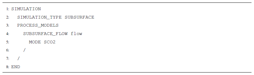
SCO2 Mode is invoked in the SUBSURFACE_FLOW block with keywords MODE SCO2 (Listing A1). To make the model isothermal, the keyword ISOTHERMAL_TEMPERATURE is used in the OPTIONS block. This model will run at a constant isothermal temperature of 45 °C.
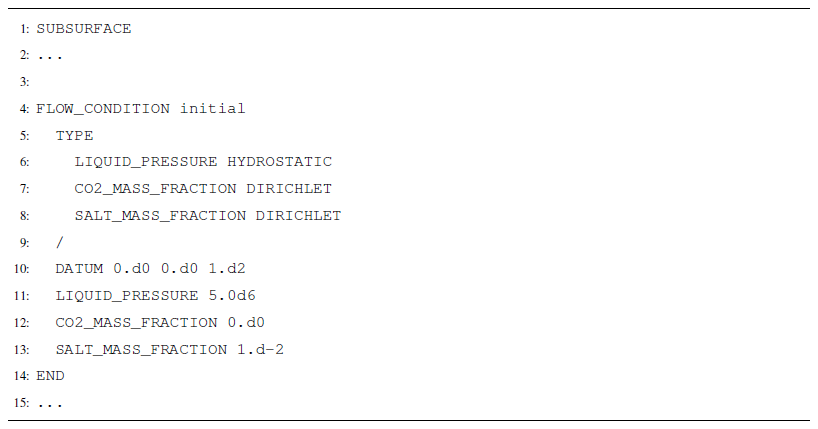
Flow conditions for the isothermal version of SCO2 Mode require three constraints (Listing A2). Constraints should be selected depending on the phase state of the flow condition. For example, if the model is to be initialized at fully aqueous-saturated conditions, a FLOW_CONDITION must be specified with LIQUID_PRESSURE, CO2_MASS_FRACTION, and SALT_MASS_FRACTION. Likewise, if an initial or boundary condition were to be in the two-phase state, a GAS_PRESSURE, LIQUID_PRESSURE, and SALT_MASS_FRACTION would be required. That is, to achieve a particular phase state for a flow condition, the constraints requested in the flow conditions must match the primary variables associated with that phase state (Table 1).
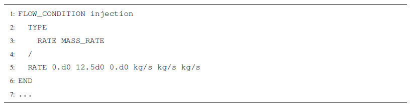
The CO2 injection is defined through a RATE type flow condition, where water mass rate, CO2 mass rate, and salt mass rate are specified followed by their corresponding units (Listing A3). More information on options for specifying injection/extraction rates can be found in Sect. A3.
A3 Well Model
Defining a well trajectory in PFLOTRAN can take several forms (see Table A3). The most general form invokes the WELL_TRAJECTORY keyword and allows the user to employ an arbitrary combination well path segments (lines and curves) to construct a well geometry of their choice. Since the well trajectory is defined first by a set of lines and curves in 3 dimensions, using this option ensures that if reservoir grid resolution is refined, the well trajectory will be refined accordingly and that well segments will properly map to reservoir cells. Defining the well trajectory always begins at the surface location of the wellhead and proceeds downward through a sequence of well intervals.
As an example, constructing the well shown in Fig. A1 would require four entries to the WELL_TRAJECTORY block: first, the SURFACE_ORIGIN would be defined (red circle in Fig. A1). Then, well interval 1 would be defined by SEGMENT_DXYZ and the corresponding dx, dy, and dz of that interval (green in Fig. A1). Next, the well transitions to horizontal in the x-dimension over a particular radius. This is achieved by using the SEGMENT_RADIUS_TO_HORIZONTAL_X keyword and the desired radius r (green in Fig. A1). Finally, a horizontal leg extending in the x-direction can be constructed with another SEGMENT_DXYZ entry. Note, this interval definition is independent of the reservoir mesh. PFLOTRAN will split each interval into its corresponding discrete well segment form (i.e., the representation in Fig. 1) internally as a function of the mesh. For curved intervals or intervals that do not move strictly in one principal direction, this can result in stair-stepping on structured grids, so users should keep this in mind when building wells. Each well interval is additionally defined as being either CASED or SCREENED; separate well intervals need to be defined accordingly. CASED intervals are disconnected from the reservoir cells through which they pass (i.e., well-reservoir flux is 0); SCREENED intervals are hydraulically connected to their reservoir cells.
On very large unstructured grids, the algorithm for constructing discrete well segments and mapping well segments to reservoir cells can be computationally costly. Therefore, whenever a well is constructed using the WELL_TRAJECTORY keyword, PFLOTRAN outputs a <well-name>_well-segments.dat text file containing all of the necessary information to import the discretized well back into the simulator for future runs. It is recommended that the user read in a well trajectory by invoking the keywords SEGMENT_LIST FILE <well-name>_well-segments.dat when running multiple models on the same reservoir mesh with the same well or wells, to speed up model runs. If the reservoir discretization changes, or if the well trajectories are adjusted, these files must be regenerated.
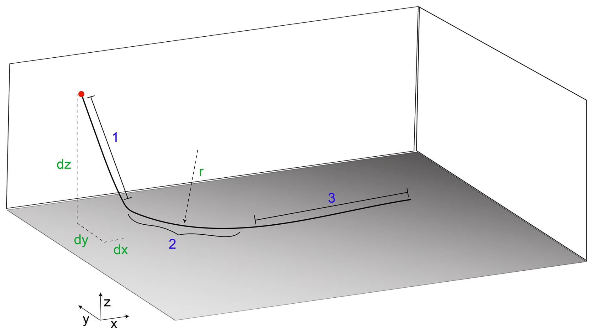
Figure A1Example well trajectory. Red: the location of the wellhead; blue: example ordering of well intervals; green: example input types
The wellbore itself is defined by several parameters. Those include the wellbore diameter, wellbore axial friction coefficient, skin factor, and well index model. The default well index model is the 3D anisotropic Peaceman model (PEACEMAN_3D). To define an upper pressure threshold, beyond which the well is treated as pressure controlled, the keyword FRACTURE_PRESSURE must be invoked followed by a value for fracture pressure. Likewise, a minimum threshold pressure can be assigned using the keyword MINIMUM_PRESSURE.
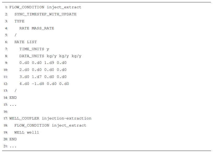
It is recommended that the user define well flow rate and composition for SCO2 Mode using a WELL_COUPLER. By invoking the USE_WELL_COUPLER keyword in the WELLBORE_MODEL block, the user can then subsequently define a FLOW_CONDITION to be applied to the well vis-a-vis the WELL_COUPLER block. Just as a BOUNDARY_CONDITION/INITIAL_CONDITION/SOURCE_ SINK block links FLOW_CONDITIONs (and TRANSPORT_CONDITIONs) to REGIONs, a WELL_COUPLER links FLOW_CONDITIONs (and TRANSPORT_CONDITIONs) to WELLs. A FLOW_CONDITION for a well contains at minimum a TYPE RATE MASS_RATE constraint, where the RATE can be defined by a single set of values or a time-dependent list of values (see PFLOTRAN Documentation, https://documentation.pflotran.org, last access: 18 December 2025, for a more detailed description of flow conditions and rate options, including interpolation options).
The RATE keyword expects the same number of entries as there are reservoir degrees of freedom. That means that for isothermal simulations, RATE expects 3 entries followed by 3 units. The order matters: the first entry is a water source or sink, the second entry is a CO2 source or sink, and the third entry is a salt source or sink. Units are mass per time. Positive numbers indicate injection. Therefore, to inject 1000 kg s−1 of pure CO2, the RATE would appear as in Listing A4.

If thermal effects are being considered, the RATE keyword expects an additional entry for energy flux. Note that this also applies to FIXED_TEMPERATURE_GRADIENT, and that the energy source term is added on top of the enthalpy of the fluid being injected. Therefore, it is most common for the energy source/sink to be 0. Units also need to be provided, typically in MW. For example, a modified RATE when running thermal simulations would appear as in Listing A5.

By default, injection temperature is set equal to the reservoir temperature at the location of the injection. Injection temperature can optionally be modified by including an additional TEMPERATURE DIRICHLET constraint in the TYPE block of the FLOW_CONDITION. Also, RATEs are treated by default as pure component mass rates. The user can optionally invoke the CO2_MASS_FRACTION DIRICHLET and RELATIVE_HUMIDITY DIRICHLET constraint types. By invoking these, PFLOTRAN will treat water mass source terms as liquid phase mass sources and partition between CO2 and H2O mass according to the CO2_MASS_FRACTION provided; likewise, a CO2 mass source will be treated as a CO2 phase mass source and partition between components according to the RELATIVE_HUMIDITY fraction. This could also be achieved by supplying two component mass rates without the need to invoke the CO2_MASS_FRACTION or RELATIVE_HUMIDITY keywords.
Negative RATE values extract mass from the reservoir through the well. Reservoir fluid temperature and composition are always used with extraction wells. Thus, the values provided are always total mass rates. Any values provided to the mass rate terms are summed, and PFLOTRAN applies that value as the total mass extraction rate applied to the model. Therefore it is recommended that users supply total mass extraction rates to the first entry of each RATE for simplicity. To extract 1000 kg s−1 of total mass in an isothermal simulation, a RATE would appear as in Listing A6.

For example, if the reservoir contains only liquid water with dissolved salt and dissolved CO2, applying this rate will extract water, CO2, and salt components where the sum of the component mass rates equals the total production rate. On the other hand, if free-phase CO2 and liquid water both coexist in the reservoir cell where the extraction is taking place, individual phase mass rates are weighted by their mobility ratios (i.e., if gas phase exists but it is immobile, only liquid phase will be extracted, and vice versa). PFLOTRAN then solves for well bottomhole pressure such that sum of total mass of water and CO2 extracted from both phases equals the user-specified extraction rate.

When running models with reactive transport, a TRANSPORT_CONDITION will define the constraints on dissolved aqueous species that are not CO2. For instance, if the user wishes to inject 1000 kg s−1 of water with a tracer in an isothermal model, the FLOW_CONDITION would read as in Listing A7. A separate TRANSPORT_CONDITION would prescribe the tracer concentration in the water.
The following example contains sections of an input deck that invoke certain well model options. Complete input decks corresponding to more complex benchmark problems can be found in Nole et al. (2025b).
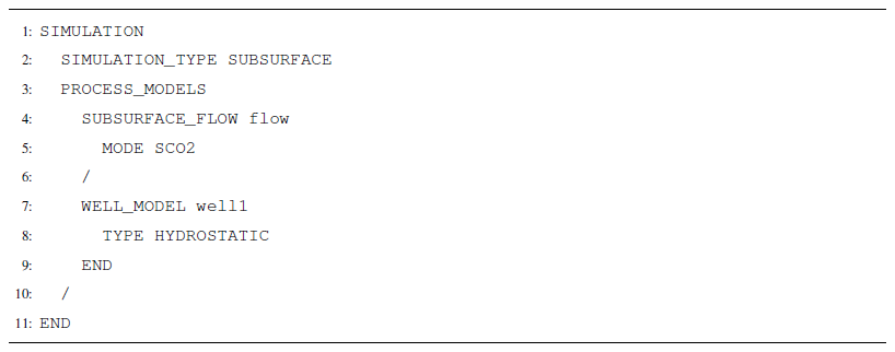
The well model is first requested by invoking WELL_MODEL in the PROCESS_MODELS block of SIMULATION (Listing A8).
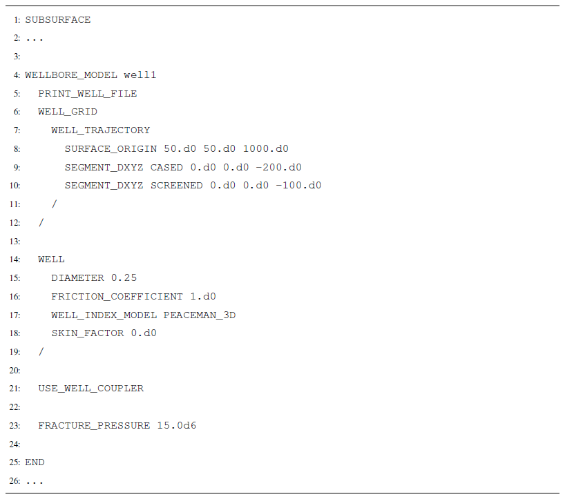
In the WELLBORE_MODEL block in SUBSURFACE, the WELL_GRID and WELL properties must be defined. Optionally, USE_WELL_COUPLER links a well to flow/transport conditions and FRACTURE_PRESSURE sets a maximum pressure threshold for pressure control (Listing A9).
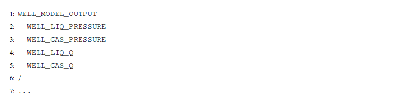
A separate WELL_MODEL_OUTPUT block defines certain well variables to include in output files (Listing A10).
Injection/extraction rates and schedules are defined in a FLOW_CONDITION and then coupled to any/all wells through a WELL_COUPLER (Listing A11).
A4 Non-isothermal Flow
Running non-isothermal models is the default behavior of SCO2 Mode. Therefore to set up a CO2 model that considers thermal effects, no additional OPTIONS are required in the SUBSURFACE_FLOW block. However, in addition to the three mass degree of freedom constraints, an additional constraint for the energy equation is also required. The fourth primary variable for all phase states is temperature; therefore, a temperature Dirichlet constraint (or energy flux Neumann constraint) is required in each FLOW_CONDITION. An example of some minimum requirements for setting up a thermal CO2 injection model are shown below.
The following example contains sections of an input deck that can be used to set up a simple CO2 injection considering thermal effects. Complete input decks corresponding to more complex benchmark problems can be found in Nole et al. (2025b).
SCO2 Mode is invoked in the SUBSURFACE_FLOW block with keywords MODE SCO2 (Listing A12). No additional options are required for a thermal model.
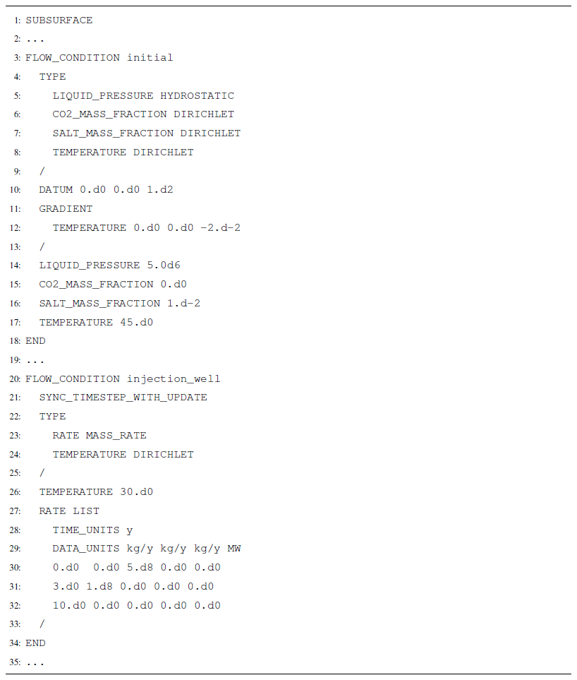
In each FLOW_CONDITION, a thermal constraint must be added (Listing A13). For temperature constraints of TYPE DIRICHLET, the user can either specify a constant temperature or the temperature at a reference datum in conjunction with a geothermal gradient. Here, the initial condition specifies a geothermal temperature gradient and a temperature at a specified datum. In an injection well, a constant temperature is specified.
A5 Reactive Transport Coupling
SCO2 Mode has been designed to couple with PFLOTRAN's reactive transport libraries for modeling coupled multiphase flow and CO2 reactivity. Invoking this coupling only requires adding a SUBSURFACE_TRANSPORT block to the PROCESS_MODELS list and including CO2 species in additional input blocks associated with reactive transport.
The following example contains sections of an input deck that can be used to set up reaction coupling with CO2 flow. Complete input decks corresponding to more complex example problems, including problems that involve geochemistry coupling, can be found in Nole et al. (2025b).
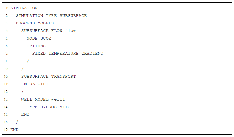
Here, SCO2 Mode is invoked in the SUBSURFACE_FLOW block, and GIRT Mode is invoked through the SUBSURFACE_TRANSPORT block (Listing A14). No additional options are required for reactive transport coupling, but the FIXED_TEMPERATURE_GRADIENT option and the WELL_MODEL block are included here as an example of possible combinations of process models.
The CHEMISTRY block and associated constraints must include CO2(aq) in order to properly enable coupling between SCO2 Mode and reactive transport (Listing A15). CO2(g) must also be included as an ACTIVE_GAS_SPECIES. This example includes the mineral calcite in its chemistry block, which is defined in a chemistry database. Specific combinations of minerals and aqueous species will depend on the desired application. The PFLOTRAN Documentation (https://documentation.pflotran.org, last access: 18 December 2025) contains more information on setting up reactive transport models, including a description of the structure of a geochemical database.
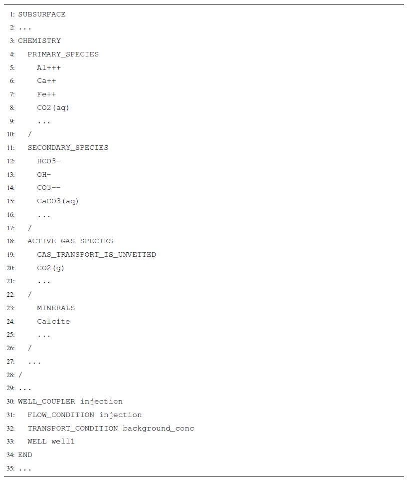
Listing A15Example Chemistry Block and Well Flow Condition for Coupled Flow and Reactive Transport Modeling.
A suite of verification tests were constructed to test individual functions, capabilities, or processes in isolation from larger, coupled, system-scale phenomena. These small, 0- and 1-dimensional test cases are designed to evaluate how well the new components developed in SCO2 Mode match their counterparts in STOMP-CO2.
B1 0D Test Cases
A set of single-cell tests cases was developed to confirm that SCO2 Mode represents the relevant CO2 equations of state, constitutive relationships, initial/boundary conditions, phase behavior, and flow/reaction coupling in a manner that is consistent with STOMP-CO2.
B1.1 CO2 Injection into a Brine Reservoir
In this test, a single grid cell is initialized at a brine pressure of 12 MPa, initial CO2 mass fraction of 0.0 kg kg−1, and initial salt mass fraction of 0.15 kg kg−1. CO2 is injected into the cell at a rate of 12.5 kg s−1. Capillary pressure is described by a Van Genuchten function with a capillary entry head of 2 m, n equal to 1.84162, liquid residual saturation of 0.3, and gas residual saturation of 0.05. A liquid phase boundary condition on the east face of the cell is set to 12 MPa, a salt mass fraction of 0.22 kg kg−1, and no dissolved CO2. An isothermal temperature of 20 °C is set in the cell. PFLOTRAN and STOMP-CO2 report identical results, verifying the implementation of CO2-brine phase partitioning, capillary pressure, salt precipitation models, and liquid phase boundary conditions in PFLOTRAN (Fig. B1).
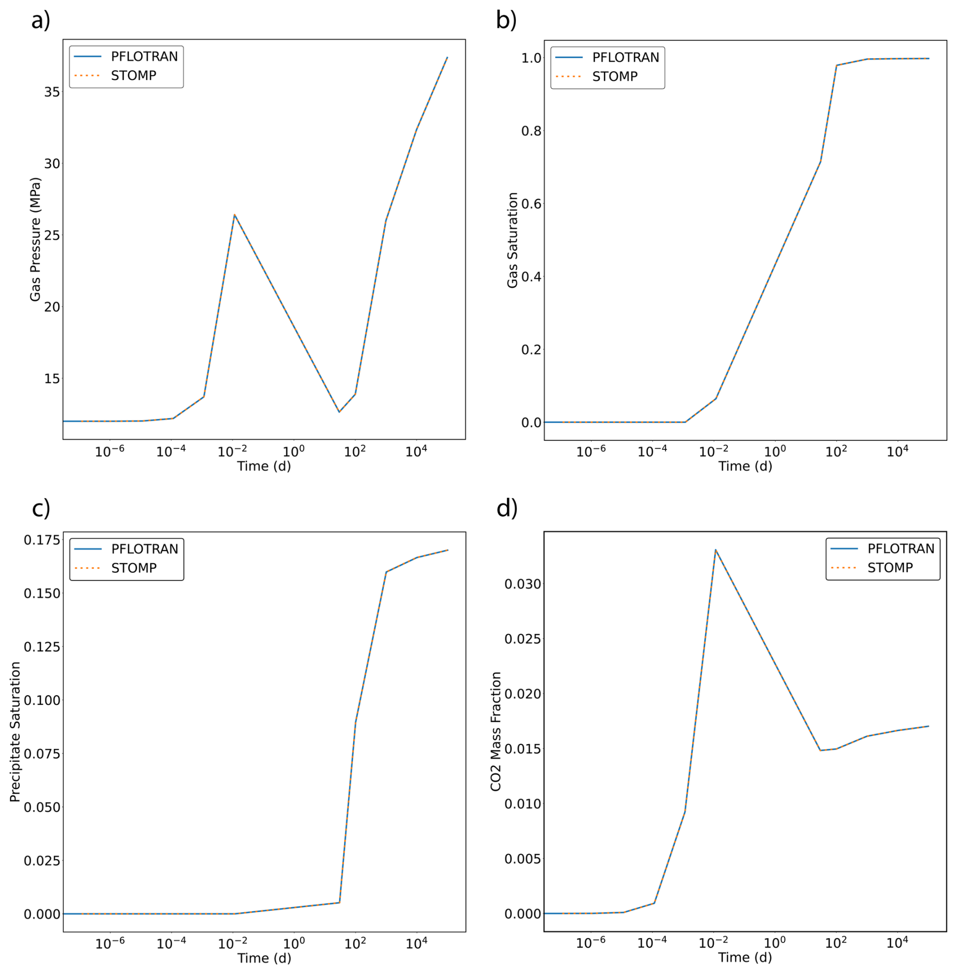
Figure B1Single-cell CO2 Injection: (a) Gas Pressure, (b) Gas Saturation, (c) Precipitate Saturation, and (d) Dissolved CO2 Mass Fraction.
B1.2 Trapped Gas Hysteresis
This single-cell test was designed to verify PFLOTRAN's implementation of trapped gas hysteresis over several drainage and imbibition cycles. In this test, a single grid cell is initialized with a brine pressure of 12 MPa, a gas phase pressure of 14 MPa, and no dissolved salt. Using a Van Genuchten capillary pressure function with an entry head of 2 m, Van Genuchten n value of 1.84162, and liquid residual saturation of 0.3, a capillary pressure of 2 MPa is equivalent to an initial gas saturation of 0.6857. In this model, trapped gas hysteresis is enabled through the capillary pressure curve's optional input field for maximum trapped gas saturation. The model is isothermal at 20 °C, and boundary conditions are applied on the west and east faces of the cell. Both boundary conditions apply a liquid pressure of 12 MPa with no dissolved CO2 or dissolved salt. Initially, the boundary conditions drive water to imbibe into the domain. After 1 year, CO2 is injected into the cell at a rate of 1.0 kg s−1, causing water to drain back out of the cell. After 2 years, the gas source is shut off, causing imbibition again. Finally, after 3 years CO2 is injected at a slower rate of 0.1 kg s−1 until the end of the simulation at 4 years. Three simulations were run with different values for maximum trapped gas saturation. PFLOTRAN and STOMP-CO2 report identical results for all simulations, verifying PFLOTRAN's implementation of trapped gas hysteresis.
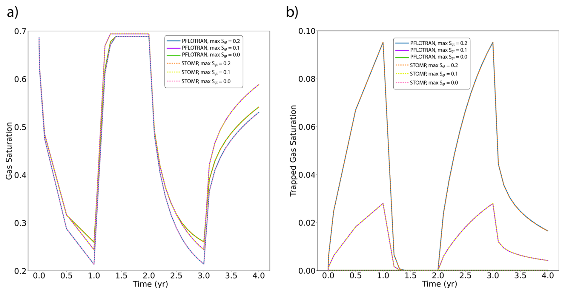
B1.3 CO2 Injection into a Reactive Brine Reservoir
This single-cell test contains a batch reactor in which a CO2 injection drives dissolution of primary minerals and subsequent carbonate mineralization. Mineral chemistry is similar to the Mineral Trapping in Basalts benchmark problem chemistry. The domain is initialized to a liquid pressure of 1 MPa, salt mass fraction of 0.01 kg kg−1, and an isothermal temperature of 24 °C. CO2 is injected at a constant rate of 1.0 × 10⁻⁵ kg s−1 for 14 d; the simulation is run for a total of 10 years. pH initially drops in the cell to around a pH of 4; PFLOTRAN and STOMP-CO2 report nearly the same pH drop. The pH then rebounds to close to pH 5 by the end of the model. PFLOTRAN and STOMP-CO2 report nearly the same pH. Primary minerals clinopyroxene and plagioclase dissolve in this model; PFLOTRAN and STOMP-CO2 report very similar dissolution of these primary minerals over the course of the 10 year simulation. PFLOTRAN and STOMP-CO2 report very similar secondary mineral mass precipitation; some differences at the point of mineral formation could be due to different timestepping in the reactive transport solve or slightly different treatment of mineral nucleation between the two reactive transport solvers. STOMP-CO2 reports nonzero masses of the least abundant secondary minerals (Dawsonite, Rhodochrosite, and Siderate), whereas PFLOTRAN reports those as zero. These mineral masses are 15 orders of magnitude smaller than the dominant secondary minerals, so they are negligible. This test problem demonstrates an implementation of flow and reactive transport coupling in PFLOTRAN that is consistent with STOMP-CO2.
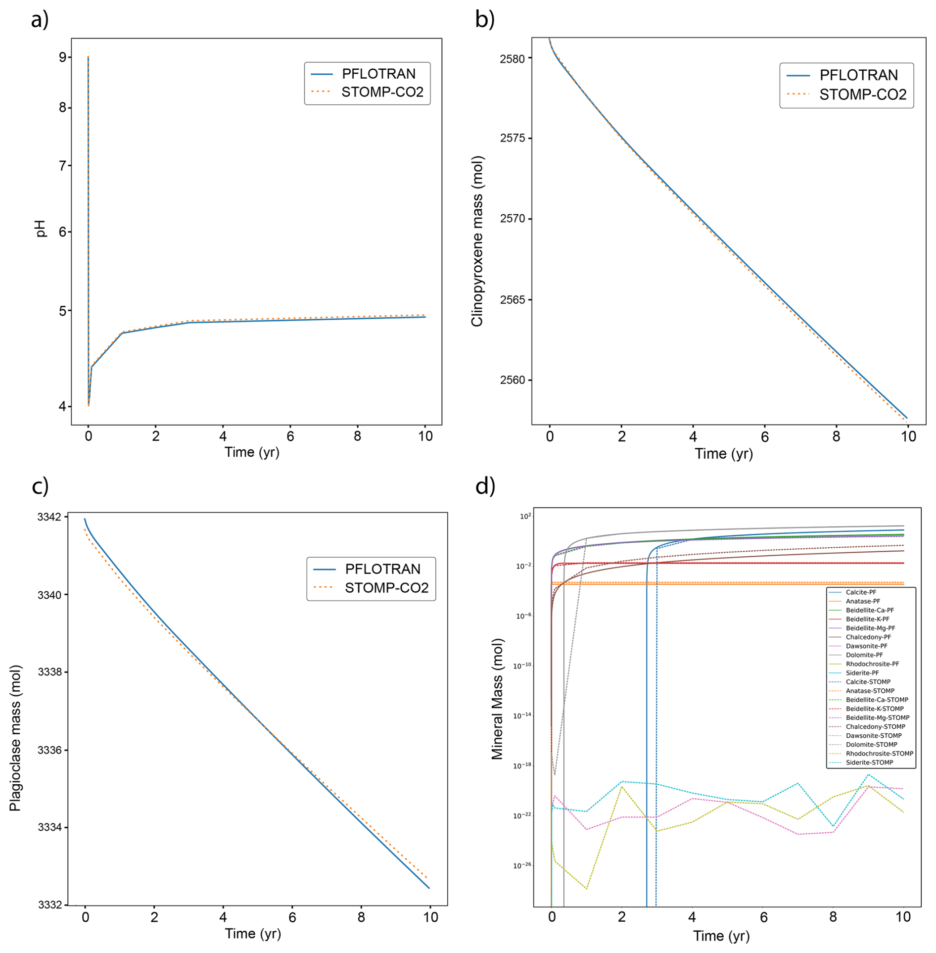
Figure B3Single-cell Reactive CO2 Injection: (a) pH, (b) Clinopyroxene, (c) Plagioclase, and (d) Secondary Minerals.
B2 1D Test Cases
Several 1D test cases were built to evaluate SCO2 Mode's representation of boundary conditions, inter-block flux terms, gravity effects, and the fully coupled well model compare to those implemented in STOMP-CO2.
B2.1 Two-Cell CO2 Injection into a Brine Reservoir
A 2-cell test problem was developed to verify the implementation of interior cell flux terms in SCO2 Mode. In this test, a 1D horizontal Cartesian model with two 15 m long grid cells is initialized to a constant liquid pressure of 12 MPa, zero dissolved CO2 mass fraction, and dissolved salt mass fraction of 0.15 kg kg−1. A source term in the left grid cell injects CO2 at 12.5 kg s−1, while a boundary condition on the right side of the model holds pressure at the initial pressure. The model is run for 1.0 × 10⁵ d. PFLOTRAN and STOMP-CO2 results at several different output times are identical, verifying the implementation of inter-cell multiphase fluxes in SCO2 Mode.
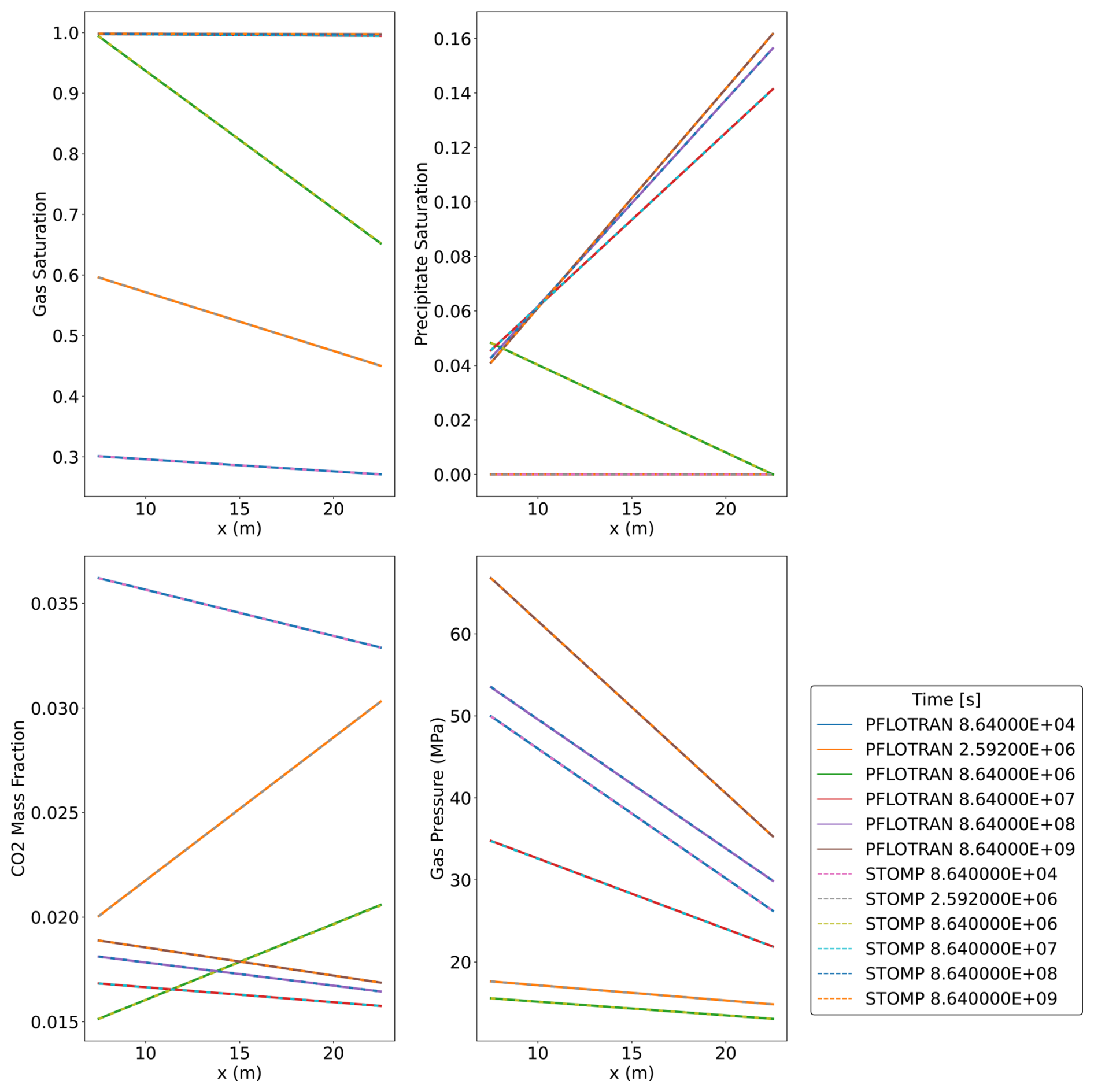
B2.2 Two-Cell CO2 Well Injection
In this test, a 2-cell Cartesian model is oriented vertically; each cell has a thickness of 100 m. A fully coupled well model injects CO2 into the domain and is screened through both cells. The well injects CO2 at a total rate of 1.0 × 10⁶ kg yr−1. Since the well is screened through both cells, mass rate of CO2 injected into each cell therefore is distributed to each cell as a function of well pressure, cell pressure, and well index. The model is initialized to a constant liquid pressure of 12 MPa and a salt mass fraction of 0.0475 kg kg−1. The top of the model is fixed at the initial liquid pressure and mass fractions; therefore, buoyancy drives upward flow of free-phase CO2 throughout the simulation and the liquid phase sinks to achieve hydrostatic pressure. The model is run to 9 × 10⁴ h. Both the PFLOTRAN and STOMP-CO2 simulations produce identical results at several output times in the simulation, verifying the implementation of the coupled well model in SCO2 Mode.
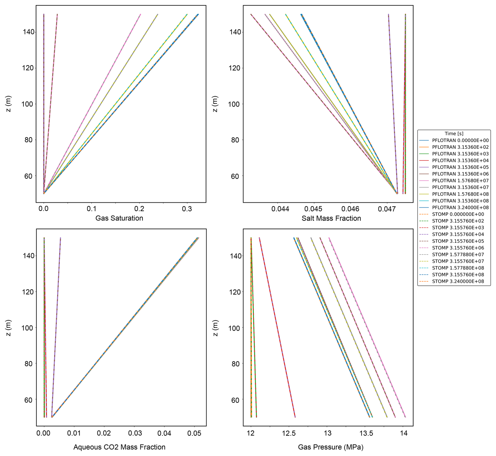
B2.3 CO2 Injection into a Vertical Brine Reservoir
This test case models a CO2 injection into a 200 m vertical column using a fully coupled well model. Here, each cell is 1 m thick; the vertical well spans the entire domain and is screened throughout. Thus, the well model injects CO2 into many more grid cells than in the previous problem. This problem tests the ability of the well model to inject into hundreds of reservoir grid cells adaptively depending on bottomhole pressure, reservoir pressure, and well index; additionally it tests the implementation of fluxes across hundreds of reservoir cells. The reservoir is initialized to a constant liquid pressure, zero CO2 mass fraction, and a constant salinity of 0.0475 kg kg−1, with a Dirichlet boundary condition at the top set at initial pressure and mass fractions. The model is isothermal at a constant temperature of 20 °C. The model is run for 9 × 10⁴ h. PFLOTRAN and STOMP-CO2 produce nearly identical results at all output times. The one exception is in dissolved CO2 mass fractions at late times in the deeper part of the model, where both simulators deviate very slightly. These results verify the implementation fully coupled wells in PFLOTRAN where the wells are screened for hundreds of grid cells.
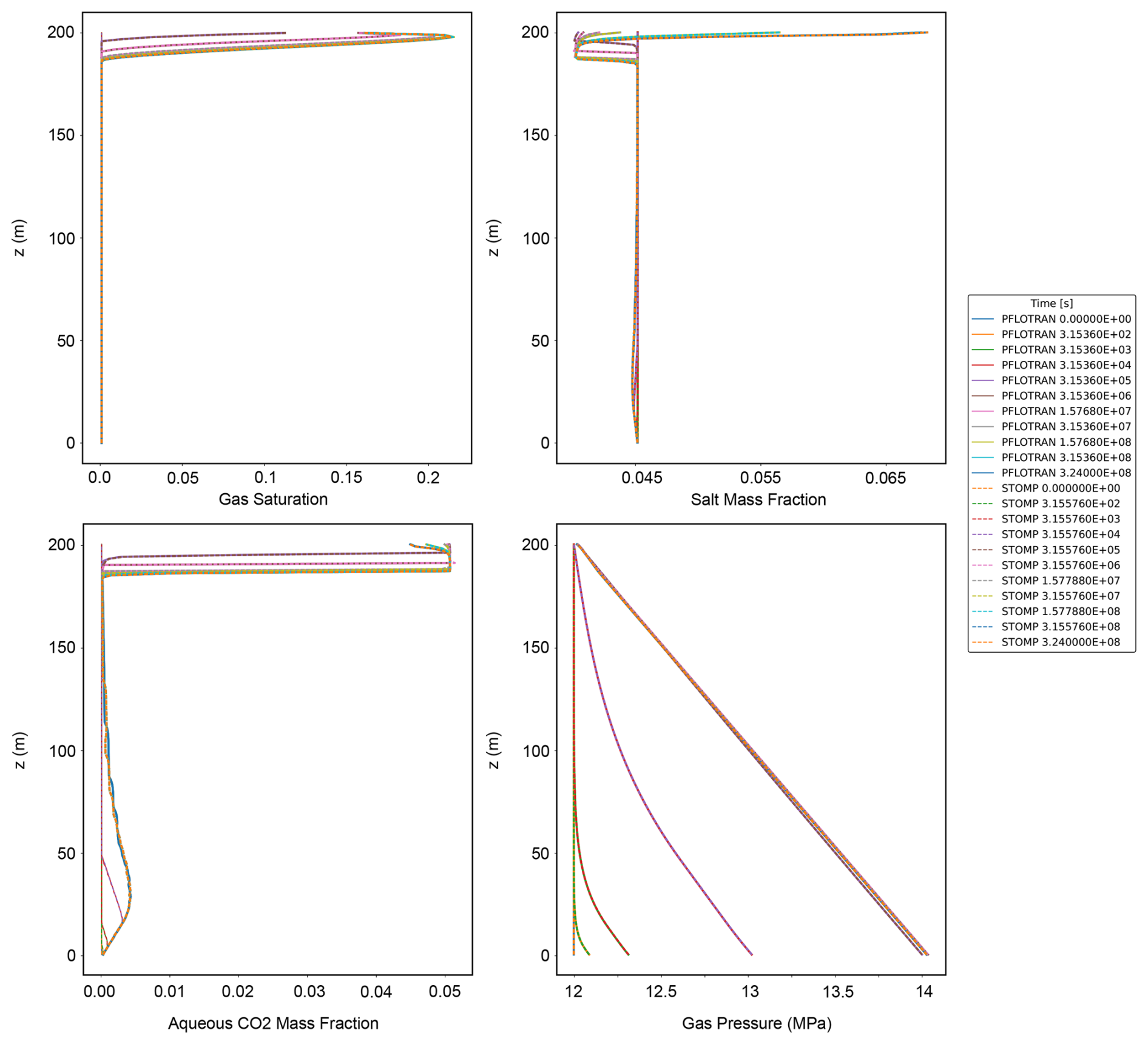
The current version of PFLOTRAN is available from the project website https://www.pflotran.org (last access: 18 December 2025) under the LGPL3 licence. The exact version of the model used to produce the results used in this paper is archived on Zenodo under https://doi.org/10.5281/zenodo.14969297, as are all input data (Nole et al., 2025b).
MN: software development, model conceptualization, formal analysis, methodology, writing; KM: model conceptualization, writing; GH: software development, review, and editing; XH: model conceptualization, writing; PL: model conceptualization, development, and writing.
The contact author has declared that none of the authors has any competing interests.
This paper describes objective technical results and analysis. Any subjective views or opinions that might be expressed in the paper do not necessarily represent the views of the U.S. Department of Energy or the United States Government.Publisher's note: Copernicus Publications remains neutral with regard to jurisdictional claims made in the text, published maps, institutional affiliations, or any other geographical representation in this paper. The authors bear the ultimate responsibility for providing appropriate place names. Views expressed in the text are those of the authors and do not necessarily reflect the views of the publisher.
This research was supported by Pacific Northwest National Laboratory's Laboratory-Directed Research and Development (LDRD) program. PNNL is operated for the DOE by Battelle Memorial Institute under contract DE-AC05-76RL01830.
This research has been supported by the Pacific Northwest National Laboratory (grant no. 211622).
This paper was edited by Ludovic Räss and reviewed by Marcos Machado and one anonymous referee.
Alendal, G. and Drange, H.: Two-phase, near-field modeling of purposefully released CO2 in the ocean, Journal of Geophysical Research: Oceans, 106, 1085–1096, 2001. a
Bartlett, R.: Solution mining: Leaching and fluid recovery of materials, Routledge, https://doi.org/10.4324/9780203357613, 2013. a
Bashir, A., Ali, M., Patil, S., Aljawad, M. S., Mahmoud, M., Al-Shehri, D., Hoteit, H., and Kamal, M. S.: Comprehensive review of CO2 geological storage: Exploring principles, mechanisms, and prospects, Earth-Science Reviews, 249, 104672, https://doi.org/10.1016/j.earscirev.2023.104672, 2024. a
Battistelli, A., Calore, C., and Pruess, K.: The simulator TOUGH2/EWASG for modelling geothermal reservoirs with brines and non-condensible gas, Geothermics, 26, 437–464, 1997. a, b
Belgodere, C., Dubessy, J., Vautrin, D., Caumon, M.-C., Sterpenich, J., Pironon, J., Robert, P., Randi, A., and Birat, J.-P.: Experimental determination of CO2 diffusion coefficient in aqueous solutions under pressure at room temperature via Raman spectroscopy: impact of salinity (NaCl), Journal of Raman Spectroscopy, 46, 1025–1032, 2015. a
Bromley, L. A.: Thermodynamic properties of strong electrolytes in aqueous solutions, AIChE Journal, 19, 313–320, 1973. a
Cadogan, S. P., Maitland, G. C., and Trusler, J. M.: Diffusion coefficients of CO2 and N2 in water at temperatures between 298.15 K and 423.15 K at pressures up to 45 MPa, Journal of Chemical & Engineering Data, 59, 519–525, 2014. a
Fayer, M. J. and Simmons, C. S.: Modified soil water retention functions for all matric suctions, Water Resources Research, 31, 1233–1238, 1995. a
Fenghour, A., Wakeham, W. A., and Vesovic, V.: The viscosity of carbon dioxide, Journal of Physical and Chemical Reference Data, 27, 31–44, 1998. a
Haas, J. L.: Physical properties of the coexisting phases and thermochemical properties of the H_2O component in boiling NaCl solution, Geol. Surv. Bull., A, 1421, 73, https://pubs.usgs.gov/bul/1421a/report.pdf (last access: 18 December 2025), 1976. a
Hammond, G. E., Lichtner, P. C., and Mills, R.: Evaluating the performance of parallel subsurface simulators: An illustrative example with PFLOTRAN, Water Resources Research, 50, 208–228, 2014. a, b, c, d, e
Harvey, O. R., Qafoku, N. P., Cantrell, K. J., Lee, G., Amonette, J. E., and Brown, C. F.: Geochemical implications of gas leakage associated with geologic CO2 storage: A qualitative review, Environmental Science & Technology, 47, 23–36, 2013. a
Kaluarachchi, J. J. and Parker, J.: Multiphase flow with a simplified model for oil entrapment, Transport in Porous Media, 7, 1–14, 1992. a
Lichtner, P. C.: Continuum model for simultaneous chemical reactions and mass transport in hydrothermal systems, Geochimica et Cosmochimica Acta, 49, 779–800, https://doi.org/10.1016/0016-7037(85)90172-3, 1985. a
Matter, J. M., Broecker, W. S., Gislason, S. R., Gunnlaugsson, E., Oelkers, E. H., Stute, M., Sigurdardóttir, H., Stefansson, A., Alfreðsson, H. A., Aradóttir, E. S., and Axelsson, G.: The CarbFix Pilot Project–storing carbon dioxide in basalt, Energy Procedia, 4, 5579–5585, 2011. a
McGrail, B. P., Schaef, H. T., Spane, F. A., Cliff, J. B., Qafoku, O., Horner, J. A., Thompson, C. J., Owen, A. T., and Sullivan, C. E.: Field validation of supercritical CO2 reactivity with basalts, Environmental Science & Technology Letters, 4, 6–10, 2017. a, b, c
Meyer, C., McClintock, R., Silvestri, G., and Spencer, R.: ASME Steam Tables, The American Society of Mechanical Engineers, New York, ISBN 9780791806326, 1993. a, b, c, d, e
Michaelides, E.: Thermodynamic properties of geothermal fluids, Trans.-Geotherm. Resour. Counc. (United States), 5, 361–364, 1981. a
Millington, R. and Quirk, J.: Permeability of porous media, Nature, 183, 387–388, 1959. a
Nitao, J. J.: Numerical modeling of the thermal and hydrological environment around a nuclear waste package using the equivalent continuum approximation: horizontal emplacement, Tech. rep., Lawrence Livermore National Lab., https://inis.iaea.org/records/x2yc8-b8g13/files/20038045.pdf (last access: 18 December 2025), 1988. a
Nole, M., Bartrand, J., Naim, F., and Hammond, G.: Modeling commercial-scale CO2 storage in the gas hydrate stability zone with PFLOTRAN v6.0, Geosci. Model Dev., 18, 1413–1425, https://doi.org/10.5194/gmd-18-1413-2025, 2025a. a
Nole, M., Muller, K., Hammond, G., He, X., and Lichtner, P.: Modeling Supercritical CO2 Flow and Mineralization in Reactive Host Rocks with PFLOTRAN v7.0: Data, Zenodo [data set], https://doi.org/10.5281/zenodo.14969297, 2025b. a, b, c, d
Nordbotten, J. M., Ferno, M. A., Flemisch, B., Kovscek, A. R., and Lie, K.-A.: The 11th Society of Petroleum Engineers Comparative Solution Project: Problem Definition, SPE Journal, 29, 2507–2524, 2024. a
Nordbotten, J. M., Fernø, M. A., Flemisch, B., Kovscek, A. R., Lie, K.-A., Both, J. W., Møyner, O., Sandve, T. H., Ahusborde, E., Bauer, S., Chen, Z., Class, H., Di, C., Ding, D., Element, D., Flauraud, E., Franc, J., Gasanzade, F., Ghomian, Y., Giddins, M. A., Green, C., Fernandes, B. R., Hadjisotiriou, G., Hammond, G., Huang, H., Kachuma, D., Kern, M., Koch, T., Krishnamurthy, P., Lye, K. O., Landa-Marbán, D., Nole, M., Orsini, P., Ruby, N., Salinas, P., Sayyafzadeh, M., Torben, J., Turner, A., Voskov, D. V., Wendel, K., and Youssef, A. A.: Benchmarking CO2 storage simulations: Results from the 11th Society of Petroleum Engineers Comparative Solution Project, International Journal of Greenhouse Gas Control, 148, 104519, https://doi.org/10.1016/j.ijggc.2025.104519, 2025. a
Parker, J. and Lenhard, R.: A model for hysteretic constitutive relations governing multiphase flow: 1. Saturation-pressure relations, Water Resources Research, 23, 2187–2196, 1987. a
Patankar, S.: Numerical heat transfer and fluid flow, CRC Press, https://doi.org/10.1201/9781482234213, 2018. a
Paul, M. J., Park, H. D., Nole, M., and Painter, S. L.: Modeling Geologic Waste Repository Systems Below Residual Saturation, Nuclear Technology, 210, 1578–1592, https://doi.org/10.1080/00295450.2023.2262294, 2024. a
Peaceman, D. W.: Interpretation of well-block pressures in numerical reservoir simulation (includes associated paper 6988), Society of Petroleum Engineers Journal, 18, 183–194, 1978. a
Peaceman, D. W.: Interpretation of well-block pressures in numerical reservoir simulation with nonsquare grid blocks and anisotropic permeability, Society of Petroleum Engineers Journal, 23, 531–543, 1983. a
Phillips, S., Igbene, A., Fair, J., Ozbek, H., and Tavana, M.: A technical databook for geothermal energy utilization, University of California, Berkeley, California, https://escholarship.org/uc/item/2v39z4tw (last access: 18 December 2025), 1981. a, b
Pogge von Strandmann, P. A., Burton, K. W., Snæbjörnsdóttir, S. O., Sigfússon, B., Aradóttir, E. S., Gunnarsson, I., Alfredsson, H. A., Mesfin, K. G., Oelkers, E. H., and Gislason, S. R.: Rapid CO2 mineralisation into calcite at the CarbFix storage site quantified using calcium isotopes, Nature Communications, 10, 1983, https://doi.org/10.1038/s41467-019-10003-8, 2019. a
Poling, B. E., Prausnitz, J. M., and O'connell, J. P.: The properties of gases and liquids, vol. 5, Mcgraw-hill New York, ISBN 9780070116825, 2001. a, b, c
Pruess, K.: On production behavior of enhanced geothermal systems with CO2 as working fluid, Energy Conversion and Management, 49, 1446–1454, 2008. a
Pruess, K., Oldenburg, C. M., and Moridis, G.: TOUGH2 user's guide version 2, Lawrence Berkeley National Laboratory, https://escholarship.org/uc/item/4df6700h (last access: 18 December 2025), 1999. a
Pruess, K., Garcia, J., Kovscek, T., Oldenburg, C., Rutqvist, J., Steefel, C., and Xu, T.: Intercomparison of numerical simulation codes for geologic disposal of CO2, Tech. rep., Lawrence Berkeley National Laboratory, LBNL-51813, Berkeley, California, https://escholarship.org/uc/item/0kv4m82z (last access: 18 December 2025), 2002. a, b, c, d, e
Raza, A., Glatz, G., Gholami, R., Mahmoud, M., and Alafnan, S.: Carbon mineralization and geological storage of CO2 in basalt: Mechanisms and technical challenges, Earth-Science Reviews, 229, 104036, https://doi.org/10.1016/j.earscirev.2022.104036, 2022. a
Sambo, C., Liu, N., Shaibu, R., Ahmed, A. A., and Hashish, R. G.: A technical review of CO2 for enhanced oil recovery in unconventional oil reservoirs, Geoenergy Science and Engineering, 221, 111185, https://doi.org/10.1016/j.petrol.2022.111185, 2023. a
Shu, J.: Comparison of various techniques for computing well index, Master’s Report, Stanford University, https://stacks.stanford.edu/file/druid:xk906gg6034/Shu05.pdf (last access: 18 December 2025), 2005. a
Span, R. and Wagner, W.: A new equation of state for carbon dioxide covering the fluid region from the triple-point temperature to 1100 K at pressures up to 800 MPa, Journal of Physical and Chemical Reference Data, 25, 1509–1596, 1996. a, b
Spycher, N. and Pruess, K.: A phase-partitioning model for CO 2–brine mixtures at elevated temperatures and pressures: application to CO 2-enhanced geothermal systems, Transport in Porous Media, 82, 173–196, 2010. a
Spycher, N., Pruess, K., and Ennis-King, J.: CO2-H2O mixtures in the geological sequestration of CO2. I. Assessment and calculation of mutual solubilities from 12 to 100 C and up to 600 bar, Geochimica et Cosmochimica Acta, 67, 3015–3031, 2003. a
Stanfield, C. H., Miller, Q. R., Battu, A. K., Lahiri, N., Nagurney, A. B., Cao, R., Nienhuis, E. T., DePaolo, D. J., Latta, D. E., and Schaef, H. T.: Carbon Mineralization and Critical Mineral Resource Evaluation Pathways for Mafic–Ultramafic Assets, ACS Earth and Space Chemistry, https://doi.org/10.1021/acsearthspacechem.4c00005, 2024. a
Verma, A. and Pruess, K.: Thermohydrological conditions and silica redistribution near high-level nuclear wastes emplaced in saturated geological formations, Journal of Geophysical Research: Solid Earth, 93, 1159–1173, 1988. a
Webb, S. W.: A simple extension of two-phase characteristic curves to include the dry region, Water Resources Research, 36, 1425–1430, 2000. a
White, M.: STOMP Shortcourse Example Problems, Tech. rep., Pacific Northwest National Laboratory, https://stomp-userguide.pnnl.gov/training/shortcourseexamples.stm (last access: 29 October 2025), 2023. a, b, c, d, e, f
White, M. D., Bacon, D. H., McGrail, B. P., Watson, D. J., White, S. K., and Zhang, Z.: STOMP subsurface transport over multiple phases: STOMP-CO2 and STOMP-CO2e guide: version 1.0, Tech. rep., Pacific Northwest National Lab.(PNNL), Richland, WA (United States), https://doi.org/10.2172/1059044, 2012. a, b
White, M. D., Bacon, D. H., White, S. K., and Zhang, Z.: Fully coupled well models for fluid injection and production, Energy Procedia, 37, 3960–3970, 2013. a
Wu, Y. and Li, P.: The potential of coupled carbon storage and geothermal extraction in a CO2-enhanced geothermal system: a review, Geothermal Energy, 8, 19, https://doi.org/10.1186/s40517-020-00173-w, 2020. a