AIRTRAC v2.0: a Lagrangian aerosol tagging submodel for the analysis of aviation SO₄ transport patterns

Aviation-induced aerosols, particularly composed of sulfate (SO₄), can interact with liquid clouds by enhancing their reflectivity and lifetime, thereby exerting a cooling effect. The magnitude of these interactions, however, remains highly uncertain and may even offset the combined warming from aviation's other climate forcers depending on spatiotemporal factors such as emission altitude and season. Here, we introduce AIRTRAC v2.0, the latest advancement of the Lagrangian tagging submodel within the Modular Earth Submodel System (MESSy), and the first submodel to provide aviation-specific sulfate tagging in this framework. AIRTRAC contributes to lowering uncertainty by tracking global contributions of aviation-emitted sulfur dioxide (SO₂) and sulfuric acid (H₂SO₄) to SO₄ formation. Using a sulfur-species tagging approach for SO₂, H₂SO₄ and SO₄, it enables the characterization of transport patterns and highlights atmospheric regions with enhanced potential for aerosol–cloud interactions. In contrast to some of the existing sulfate tagging models, AIRTRAC considers a full range of microphysical processes along trajectories. To investigate sulfate transport from aviation, two global simulations were performed for January–March and July–September 2015, using pulse emissions of SO₂ and H₂SO₄ distributed across a cruise altitude of 240 hPa (∼ 10.6 km) based on the aviation SO₂ inventory of the Coupled Model Intercomparison Project Phase 6 (CMIP6). Comparisons of AIRTRAC-derived SO₄ distributions with perturbation-based simulations under analogous conditions show reasonable agreement. Using AIRTRAC v2.0, we estimate median SO₂ and SO₄ lifetimes of 22 d and 2.1 months, respectively, in northern winter, and 14 d and 2.2 months in summer, consistent with volcanic eruption modeling studies and observational benchmarks involving high-altitude SO₂ injection. The median SO₄ production efficiency during summer was found to be statistically significantly larger by 144 % compared to winter, likely due to a more efficient oxidation of SO₂. Large-scale circulation patterns and emission latitude may enhance SO₄ lifetimes: tropical emissions can be upwelled into the stratosphere past 100 hPa (∼ 16 km) over time, while high-latitude emissions can persist longer because they may be directly injected above the climatological tropopause. AIRTRAC v2.0 currently excludes SO₂ oxidation from aviation nitrogen oxides (NO_x) and does not tag other species such as black carbon. Owing to its flexible design, however, the approach can be readily extended to additional aerosols. Overall, AIRTRAC v2.0 offers the novel capability to track the atmospheric transport of aviation-emitted SO₂, H₂SO₄ and SO₄, providing critical insights into one of aviation's most uncertain climate impacts.

1 Introduction

Recent estimates suggest that in 2018, aviation accounted for approximately 2 % of the total anthropogenic radiative forcing (RF) from carbon dioxide (CO₂; Klöwer et al., 2021) and about 3.5 % or ∼ 150 mW m⁻² (70–229 mW m⁻² for a 90 % central interval) of all anthropogenic warming when additional non-CO₂ effects (Lee et al., 2021) are also contemplated. The latter estimate, however, carries significant uncertainties due to the complex interactions and trade-offs between various climate forcers, including nitrogen oxides (NO_x), water vapor (H₂O) and persistent contrails. Additionally, this estimate includes warming and cooling from direct absorption and scattering effects of soot (black carbon (BC) and organic carbon (OC)) and sulfate (SO₄) aerosols, respectively. However, it does not consider any indirect RF contributions from their interaction with clouds. Furthermore, Lee et al. (2021) do not include the potential influence of aviation NO_x on SO₄ and nitrate (NO₃) aerosol formation, both of which may contribute with substantial cooling (Terrenoire et al., 2022).

Notably, the indirect cooling effect of SO₄ aerosols alone could reduce aviation's net radiative forcing considerably. Some estimates indicate that the absolute value of this cooling effect may range from 17 to 160 mW m⁻² (Gettelman and Chen, 2013; Kapadia et al., 2016; Fig. 5 in Lee et al., 2021), a magnitude comparable to aviation's largest global mean warming contribution from aircraft-induced contrail cirrus, estimated at 111 [33, 189] mW m⁻² for 2018 (Lee et al., 2021) and 62 mW m⁻² for 2019 (Teoh et al., 2024). These indirect aerosol effects raise the possibility of a near-zero or even net negative radiative forcing (RF) from kerosene-powered aircraft. However, this outcome remains highly uncertain due to the inherent complexities in their quantification. More robust estimates from independent modeling efforts, supported by a better understanding of critical processes such as pollutant transport patterns, are essential. Without clearer insights into these climate forcers, the effective development and comprehensive evaluation of mitigation strategies will remain challenging.

Aerosols are collections of solid or liquid particles suspended in the atmosphere, with sizes ranging from 0.001 to 100 µm (Petzold and Kärcher, 2012; Brasseur and Jacob, 2017). Among the aerosols resulting from aviation are soot and sulfate. Soot is produced from the incomplete combustion of aromatic compounds in the jet fuel (Kärcher et al., 2007; Lee et al., 2021), while SO₄ forms indirectly from the emissions of sulfur dioxide (SO₂) and sulfuric acid (H₂SO₄). Experimental studies indicate that aircraft convert approximately 97 %–98 % of the fuel sulfur content into SO₂, with SO₂ emissions nearly directly proportional to fuel sulfur levels. The remaining 2 %–3 % is emitted as H₂SO₄ (Petzold et al., 2005; Jurkat et al., 2011; Owen et al., 2022). The gaseous conversion of SO₂ to H₂SO₄ involves a series of reactions (Reactions R1–R3), where the oxidation of SO₂ by hydroxyl (OH) radicals eventually results in the production of H₂SO₄ (Mikkonen et al., 2011):

$$\begin{array}{}\text{(R1)}& {\displaystyle }{\mathrm{SO}}_{\mathrm{2}}+\mathrm{OH}\to {\mathrm{HSO}}_{\mathrm{3}}\text{(R2)}& {\displaystyle }{\mathrm{HSO}}_{\mathrm{3}}+{\mathrm{O}}_{\mathrm{2}}\to {\mathrm{SO}}_{\mathrm{3}}+{\mathrm{HO}}_{\mathrm{2}}\text{(R3)}& {\displaystyle }{\mathrm{SO}}_{\mathrm{3}}+\mathrm{2}{\mathrm{H}}_{\mathrm{2}}\mathrm{O}\to {\mathrm{H}}_{\mathrm{2}}{\mathrm{SO}}_{\mathrm{4}}+{\mathrm{H}}_{\mathrm{2}}\mathrm{O}.\end{array}$$

The formation of SO₄ aerosols can proceed through multiple mechanisms. One pathway involves the condensation of H₂SO₄ vapor onto pre-existing particles, followed by particle growth through coagulation and further condensation (Whitby and McMurry, 1997; Laaksonen et al., 2000; Aquila et al., 2011). Sulfate aerosols may also form via the binary homogeneous nucleation between H₂SO₄ and H₂O, a process influenced by factors such as atmospheric relative humidity and temperature (Vehkamäki et al., 2002; Kaiser et al., 2014). Additionally, SO₄ production can occur through the reaction of H₂SO₄ with gaseous ammonia (NH₃), resulting in the formation of ammonium sulfate ((NH₄)₂SO₄) or ammonium bisulfate (NH₄HSO₄), which subsequently dissociate to yield SO₄, ammonium (NH₄) and hydrogen (Khoder, 2002). The dominant pathway, however, involves the liquid-phase oxidation of sulfurous acid (H₂SO₃) by hydrogen peroxide (H₂O₂) and ozone (O₃; Martin and Damschen, 1981; Yang et al., 2017). Figure 1 illustrates the primary reaction mechanisms leading to SO₄ formation via SO₂ and H₂SO₄.

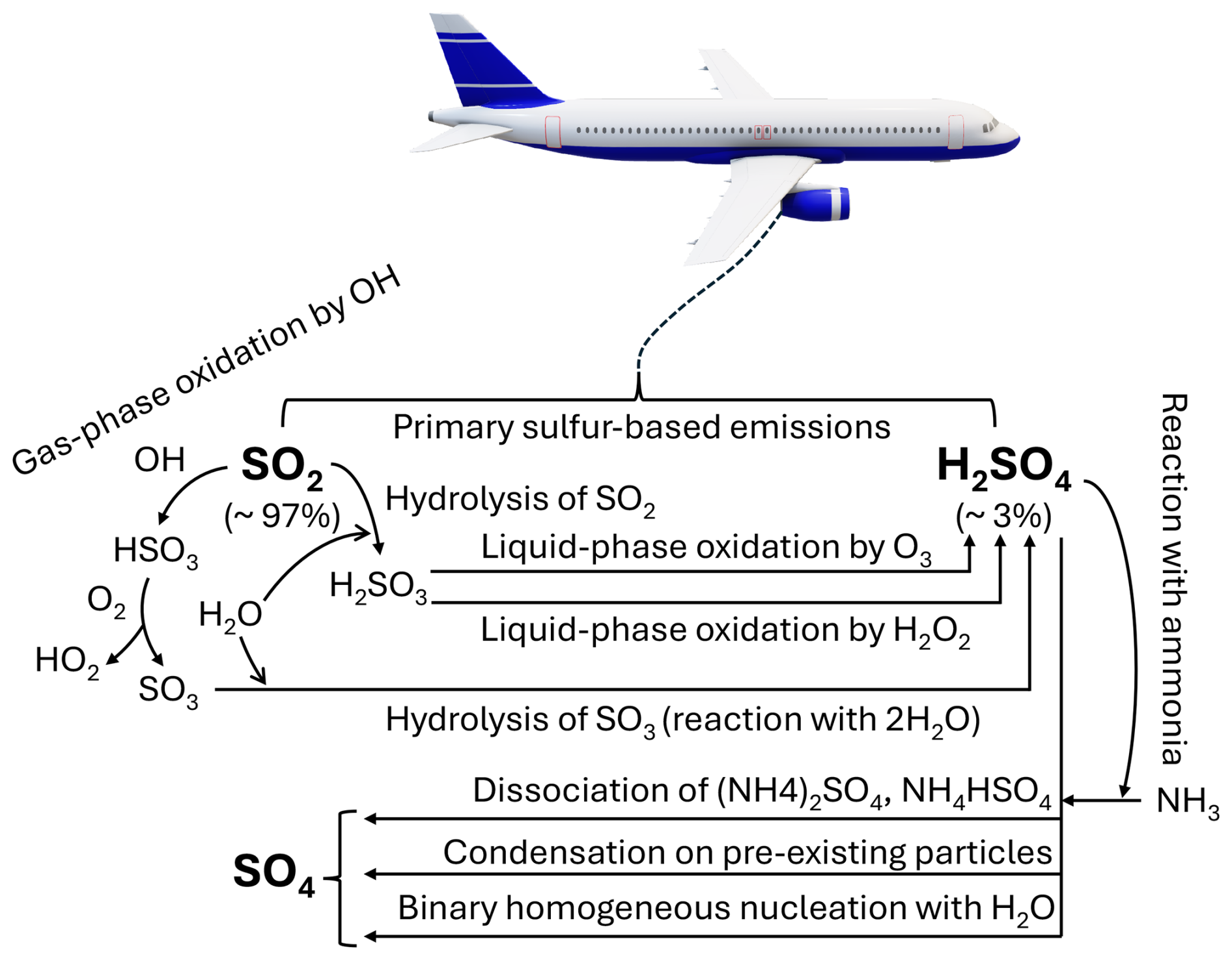
Figure 1 Production mechanisms of sulfate (SO₄) from aviation emissions of sulfur dioxide (SO₂) and sulfuric acid (H₂SO₄). The percentages indicate the conversion amount of aviation fuel sulfur content into SO₂ and H₂SO₄.

Sulfate aerosols directly alter the Earth's energy balance by scattering primarily incoming shortwave solar radiation, resulting in a cooling effect, whereas soot particles predominantly absorb this radiation, leading to a warming effect (Haywood and Shine, 1995; Kirkevåg et al., 1999; Lee et al., 2021). Additionally, these aerosols also exert indirect effects by modifying cloud microphysics. By acting as cloud condensation nuclei (CCN), increased particle number can raise cloud droplet number concentration (CDNC) and reduce droplet size for a constant liquid water content, thereby increasing liquid cloud albedo (Twomey, 1977; Lohmann and Feichter, 1997; Sausen et al., 2012). Smaller droplets may also lead to the suppression of precipitation and can prolong cloud lifetime (Albrecht, 1989; Lohmann and Feichter, 2005).

These aerosol-cloud interactions have large uncertainties that stem, in part, from the challenge in representing sub-grid scale cloud microphysical processes in global climate models (Lohmann and Feichter, 1997, 2005). More specifically, limited understanding of aerosol transport pathways, including vertical transport, large-scale horizontal advection and variations in microphysical and removal processes along these paths contribute to this uncertainty (Barrie et al., 2001; Weinzierl et al., 2017). These transport dynamics are particularly relevant for aviation emissions, as the higher emission location significantly enhances both the production efficiency and atmospheric lifetime of pollutants, as has been shown for NO_x emissions by Maruhashi et al. (2022). Model intercomparison initiatives, such as the Comparison of Large-Scale Sulfate Aerosol Models (COSAM), have demonstrated that the conversion of SO₂ to SO₄ is challenging to predict, resulting in a wide spread of model results between 10 %–50 % and discrepancies of up to a factor of two compared to observational data from aircraft campaigns. This spread leads to uncertainties not only in the vertical distribution profiles of SO₄, but also in the resulting number of CCN, both of which directly influence SO₄ indirect forcing (Barrie et al., 2001; Penner et al., 2001). Such knowledge gaps therefore prevent a comprehensive assessment of aviation's net climate impact (Lee et al., 2021).

Existing model intercomparisons and aviation-specific assessments have predominantly used perturbation approaches, leaving open how results might differ when using source apportionment methods like tagging to attribute sulfate and its cloud impacts back to aviation. Tagging involves labelling chemical species and reactions of interest and accompanying their fate throughout a simulation (Wang et al., 2009). It is normally applied to quantify the contribution of a sector to the total concentration of a pollutant. The perturbation method, on the other hand, involves evaluating the marginal impact of a change in emissions typically by subtracting two simulations: one with all emissions and another with changed emissions (Blanchard, 1999; Hoor et al., 2009; Clappier et al., 2017). To the authors' best knowledge, aviation-specific indirect effects of SO₄ have thus far only been estimated using the perturbation method. We have compiled a summary table (Table S1 in the Supplement) of recent modeling studies focusing on aviation and found that none have applied tagging. While perturbation is a useful method, it is insufficient on its own for formulating robust mitigation policies. Tagging techniques enable precise attribution of emissions to specific sectors, helping to identify those with the highest mitigation potential. The perturbation method can then complement this by quantifying the impacts of targeted reduction measures (Mertens et al., 2018).

Only a handful of Eulerian and Lagrangian sulfate tagging schemes exist however, due to the challenges of tracking complex liquid- and gas-phase transformations and aerosol interactions with clouds (Righi et al., 2023). Eulerian model studies, for instance, include Yang et al. (2017), who applied the Community Atmosphere Model (CAM) within the Community Earth System Model (CESM) framework to quantify global SO₄ contributions from 16 sources and assess both direct and indirect radiative forcing effects between 2010–2014. Other Eulerian tagging approaches have targeted regional impacts in China. For example, Wu et al. (2017) utilized an online tagging method within the Nested Air Quality Prediction Model System (NAQPMS) to reveal that SO₄ levels in Shanghai were significantly influenced by non-local sources. Similarly, Itahashi et al. (2017), employing the Particulate Source Apportionment Technology (PSAT) algorithm (Wagstrom et al., 2008) with the sixth version of the Comprehensive Air quality Model (CAMx), assessed SO₄ contributions from 31 Chinese provinces and found that emissions from the central and northern regions notably affected sulfate levels in Taiwan, Korea and Japan. Lagrangian tagging approaches include the study by Riccio et al. (2014), which used the Hybrid Single-Particle Lagrangian Integrated Trajectory (HYSPLIT) model to show that PM_2.5 levels in Naples were substantially impacted by emissions from other parts of Europe and dust transport from the Sahara. There are also Lagrangian particle dispersion models like FLEXible PARTicle (FLEXPART) and the Lagrangian Analysis Tool (LAGRANTO) that have been applied to study sulfate from volcanic emissions (Sun et al., 2023, 2024; Toohey et al., 2025). These studies are somewhat comparable to the scenario of aircraft cruise emissions, as both emit SO₂ above sea level and may inject SO₄ into the upper troposphere and lower stratosphere (UTLS). None of these studies, however, have characterized the aviation-specific global transport patterns of SO₄ originating from the primary emissions of SO₂ and H₂SO₄ introduced at subsonic cruise altitudes.

We address this fundamental knowledge gap by introducing the first Lagrangian aerosol tagging submodel for SO₄ within the fifth-generation European Centre for Medium-Range Weather Forecasts – Hamburg (ECHAM)/Modular Earth Submodel System (MESSy) Atmospheric Chemistry (EMAC) modeling framework, enabling a detailed, parcel-by-parcel analysis of aviation SO₄ transport patterns. AIRTRAC v2.0 represents an important advancement, extending the original AIRTRAC submodel (Supplement of Grewe et al., 2014a) by incorporating aerosol microphysical processes along air parcel trajectories. Specifically, aerosol mixing ratios are computed using the extensively validated third-generation Modal Aerosol Dynamics model for Europe (MADE3; Kaiser et al., 2014, 2019) submodel, while aviation-specific contributions are quantified by AIRTRAC. Previously, AIRTRAC was limited to the study of gas-phase emissions such as NO_x and H₂O (Frömming et al., 2021; Maruhashi et al., 2022) and primarily aimed at quantifying their contributions to atmospheric concentrations of reactive nitrogen species (NO_y), including nitric acid (HNO₃), O₃, the hydroperoxyl radical (HO₂), the hydroxyl radical (OH) and methane (CH₄). This Lagrangian approach offers a substantial computational advantage over more resource-intensive Eulerian simulations by enabling the simultaneous analysis of multiple emission scenarios (Maruhashi et al., 2024).

In the present assessment, we focus on the SO₄ aerosol, as it has been shown to be a highly efficient CCN for liquid clouds. In contrast, soot is hydrophobic and therefore generally becomes a CCN only when mixed internally with other hygroscopic aerosols, like SO₄ (Kristjánsson, 2002; Lee et al., 2021). This study has three primary objectives. First, it describes a novel Lagrangian aerosol-tagging submodel and the assumptions underlying its formulation. Second, the study demonstrates the usefulness of the new AIRTRAC v2.0 submodel in improving our understanding of the transport patterns of aviation-induced SO₂ and H₂SO₄, particularly in identifying where these lead to the largest SO₄ enhancements, especially over regions with abundant low-level liquid clouds. The analysis considers 28 globally distributed emission points along major present-day flight routes at a typical cruise altitude (240 hPa ≈ 10.6 km) for both winter and summer. Using ESA satellite data to locate regions of significant liquid cloud cover, AIRTRAC v2.0 is applied to track trajectories most likely to interact with these clouds, highlighting its potential to inform assessments of aerosol-cloud interactions. Third, the study compares the spatial distributions of SO₄ generated by this tagging approach against those derived from a perturbation method using a similar simulation setup. As part of our evaluation, we compare our SO₂ and SO₄ lifetime estimates with those reported in other Lagrangian modeling and observational studies of volcanic eruptions. The paper is structured into six sections: Sect. 1 provides an introduction; Sect. 2 describes the overall EMAC modeling setup, including the MADE3 submodel with which AIRTRAC v2.0 has been coupled within the MESSy framework, and presents the general formulation of the SO₄ mass transport equations. Section 3 outlines the AIRTRAC v2.0 infrastructure and details the tagging formulation of the SO₄ transport equations. Section 4 presents results of simulations from AIRTRAC v2.0 and combines satellite cloud data to illustrate the submodel's capability to predict interactions with low-level liquid clouds. Section 5 compares AIRTRAC's output with the results of a perturbation approach and with prior studies. Finally, Sect. 6 summarizes key findings, considers limitations of the AIRTRAC v2.0 submodel and offers directions for future research.

2 Modeling framework

This section summarizes the most relevant characteristics of EMAC along with the main submodels applied in our base modeling setup (Sect. 2.1). Section 2.2 describes the SO₂ and H₂SO₄ pulse emission locations and emission inventory used in our simulations. In Sect. 2.3, the submodel responsible for computing aerosol microphysics (MADE3) and the general formulation of the SO₄ mass transport equations are presented. The submodels specific to the removal and transport processes of aerosols are then presented in Sect. 2.4.

2.1 The EMAC model setup

Chemistry-climate simulations in this assessment are performed with the EMAC model. It is a flexible, global model that simulates a plethora of atmospheric processes with interactions between land, ocean and anthropogenic activity via a coupling interface called MESSy (Jöckel et al., 2010) that can connect more than 100 different submodels to ECHAM5, EMAC's base general circulation model (Roeckner et al., 2006). Apart from AIRTRAC, which estimates the contribution of aviation-related pollutants along air parcel trajectories and MADE3, which calculates aerosol dynamics and microphysical processes, there are other submodels that are also relevant in our modeling setup. The full list of applied submodels is included in Table A1 in Appendix A.

Simulations are performed with version 5.3.02 of the base model ECHAM5 and with version 2.55.2 of the MESSy framework. The EMAC model resolution is T42L41DLR, which corresponds to a quadratic Gaussian grid of size ∼ 2.8° × 2.8° (with 128 longitude and 64 latitude grid cells) with 41 discrete, vertical hybrid sigma-pressure levels ranging from the surface to the uppermost layer of the atmosphere centered at 5 hPa. Across the midlatitudes and Tropics, most T42L41 model layers lie in the troposphere. At the Equator, for example, ∼ 80 % of the layers are below the climatological tropopause during July to September. Defining the UTLS here as 100–400 hPa, approximately 16 model layers fall within this pressure range (Fig. S13 of the Supplement). For comparability purposes with Righi et al. (2023), our model output is set to a temporal resolution of 11 h with a model calculation time-step length of 15 min. The meteorology (the temperature, the wind divergence, the vorticity and the logarithm of the sea-level pressure) in our simulations has been nudged by Newtonian relaxation towards ERA-Interim reanalysis data (Dee et al., 2011) for the simulated year. Sea surface temperature and sea ice concentration have been prescribed from the ERA-Interim reanalysis data as well. Two simulations (starting on 1 January and on 1 July 2015) were performed to accompany the transport of aviation SO₂ and H₂SO₄ and their chemical conversion into SO₄ for three months across 28 emission points (Fig. 2) at an altitude of 240 hPa (Fig. 3). To ensure background meteorological conditions are in quasi-equilibrium, each simulation was preceded by a four-month spin-up period. Each emission point releases variable amounts of SO₂ and H₂SO₄ in the form of 15 min pulse emissions. These are initially advected by 50 air parcels originating from the grid box of each emission point, consistent with the recommendation of Grewe et al. (2014a). These 50 air parcels are pseudo-randomly initialized around the coordinates of an emission point according to a uniform distribution between 0 and 1. A simplified background chemistry mechanism is applied with the MECCA submodel (Sander et al., 2019) for the troposphere that involves the most relevant gaseous species like NO_x, HO_x, CH₄ and O₃. Aqueous-phase chemistry is handled by the SCAV submodel (Tost et al., 2006). These chemistry mechanisms are solved automatically by the Kinetic Pre-Processor (KPP) software using Fortran 90 code (Sander et al., 2005). The overall Lagrangian setup is similar to the one used by Maruhashi et al. (2022, 2024), while the applied aerosol chemistry and scavenging mechanisms are the same as those applied by Righi et al. (2023).

2.2 SO₂ and H₂SO₄ emission points

The 28 emission locations at which SO₂ and H₂SO₄ pulses are introduced (Fig. 2) are selected to reflect a realistic modern-day spatial distribution of aviation emissions. This distribution was determined according to the 2015 CMIP6 (Feng et al., 2020) aviation emissions inventory that includes the correction for the latitudinal bias found by Thor et al. (2023). The exact coordinates of the 28 points in Fig. 2 are included in Table B1 from Appendix B. Each coordinate has three dimensions – latitude, longitude and altitude – which are found by identifying the locations at which the aviation SO₂ mass flux (kg m⁻³ s⁻¹) is maximum. The emission altitude is determined by establishing the pressure level at which the zonally averaged aviation SO₂ mass flux, which is a function of both latitude and altitude, is the largest (Fig. 3): 238.2≈240 hPa.

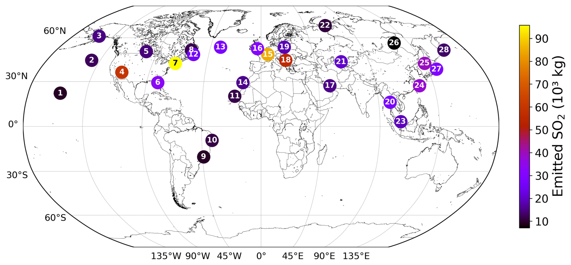
Figure 2 The 28 emission points at which SO₂ and H₂SO₄ are emitted are represented as numbered circles. This horizontal distribution of points is shown for a pressure altitude of 240 hPa (∼ 10.6 km). The amounts emitted at each point vary according to the CMIP6 aviation emissions inventory and are distinguished by the color bar. The exact coordinates and emitted amounts for SO₂ and H₂SO₄ are specified in Table B1 of Appendix B.

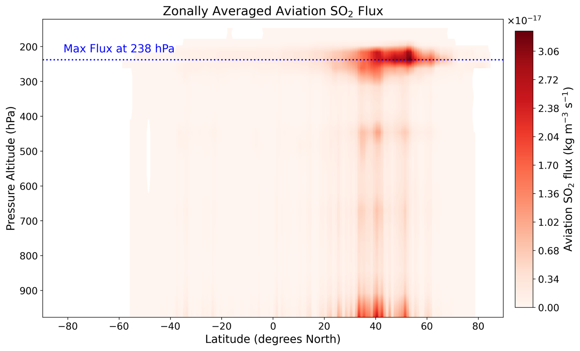
Figure 3 Altitudinal variation of the zonally averaged aviation SO₂ mass flux [kg m⁻³ s⁻¹] from the CMIP6 aviation emissions inventory. The blue dotted line represents the pressure altitude of 238.2 hPa (∼ 10.6 km) at which the maximum flux occurs.

We have developed an accompanying Python tool (see EP_selector in Appendix B and the data repository of Maruhashi et al. (2025a) for the complete code) that approximates continuous emissions as a set of distributed pulse emissions by automatically identifying the top 28 points whose grid cells have the largest SO₂ mass flux contributions (defined as a grid cell's area-weighted mean mass flux, see Eq. B1) within a user-defined mesh. The total mass of emitted SO₂ and H₂SO₄ across these points was scaled to yield the approximate global aviation SO₂ produced in a day from aviation in 2015 (Righi et al., 2023). The emitted amount of H₂SO₄ at any given emission point is determined by assuming that it constitutes 2 % of the total SO₂ mass emitted by aviation, which is consistent with measurements of aircraft exhaust plumes at cruise altitudes (Jurkat et al., 2011). Based on this assumption, the amount of H₂SO₄ emitted per simulation is found according to Eq. (B3) in Appendix B.

2.3 The MADE3 submodel and the SO₄ mass transport equations

Aerosol microphysical processes are simulated using the MADE3 (Kaiser et al., 2014, 2019) submodel, a successor of the MADE (Ackermann et al., 1998; Lauer et al., 2005) and MADE-in (Aquila et al., 2011) submodels. The performance of MADE3 has been extensively evaluated. Its ground-level aerosol mass concentrations have been compared to data from a network of measurement stations and satellite observations. Its simulated vertical profiles of the mass mixing ratios and particle number distributions have been evaluated against aircraft campaign data. Overall, the model has demonstrated satisfactory alignment with observational data, although MADE3 tends to produce larger average sulfate concentrations near the surface, with biases ranging from 13 % to 92 % when compared to observations from measurement stations (Kaiser et al., 2019).

The MADE3 submodel considers nine types of aerosols: SO₄, BC, sea spray (Na), H₂O, chloride (Cl), mineral dust (DU), NH₄, NO₃ and particulate organic matter (POM). Each aerosol type is further classified into nine modes, which result from the combination of three size categories (Aitken (subscript “k”), accumulation (subscript “a”) and coarse (subscript “c”)) and three mixing states (soluble (subscript “s”), insoluble (subscript “i”) and mixed (subscript “m”)). MADE3 therefore adopts a modal approach, where the total particle number distribution n(ln D) of an aerosol is obtained by the superposition of its nine lognormal distributions (one for each mode M), according to Eq. (1a) (Aquila et al., 2011; Kaiser et al., 2014; Boucher, 2015):

$$\begin{array}{}\text{(1a)}& n\left(\ln D\right)=\sum _{M=\mathrm{1}}^{\mathrm{9}}{\displaystyle \frac{N_M}{\sqrt{\mathrm{2}\mathit{\pi }}\ln {\mathit{\sigma }}_{\mathrm{g},M}}}\exp \left[-{\displaystyle \frac{{\left(\ln D-\ln D_{\mathrm{g},M}\right)}^{\mathrm{2}}}{\mathrm{2}{\ln }^{\mathrm{2}}{\mathit{\sigma }}_{\mathrm{g},M}}}\right],\end{array}$$

where N_M is the total particle number concentration for mode M, D_g,M is the median diameter and σ_g,M is the geometric standard deviation. Assuming spherical particles, the mass distribution m(ln D) is obtained by multiplying Eq. (1a) by the particle density ρ_M and cubic diameter D³ according to Eq. (1b):

$$\begin{array}{}\text{(1b)}& m\left(\ln D\right)=\sum _{M=\mathrm{1}}^{\mathrm{9}}{\displaystyle \frac{\mathit{\pi }}{\mathrm{6}}}{\mathit{\rho }}_M{D}^{\mathrm{3}}{\displaystyle \frac{N_M}{\sqrt{\mathrm{2}\mathit{\pi }}\ln {\mathit{\sigma }}_{\mathrm{g},M}}}\exp \left[-{\displaystyle \frac{{\left(\ln D-\ln D_{\mathrm{g},M}\right)}^{\mathrm{2}}}{\mathrm{2}{\ln }^{\mathrm{2}}{\mathit{\sigma }}_{\mathrm{g},M}}}\right].\end{array}$$

The Aitken mode is the smallest size range resolved by MADE3 and consists of particles around 10 nm, the accumulation mode includes aerosols roughly 100 nm in diameter, and the coarse mode is the largest, with particle sizes of ∼ 1 µm (Kaiser et al., 2014). Figure 4 describes the differences across the three mixing states for SO₄. The soluble state (Fig. 4a) consists entirely of soluble species like SO₄, NO₃ or others. Externally mixed or insoluble (Fig. 4b) aerosols contain a non-volatile core (e.g. black carbon or mineral dust) with a total soluble mass fraction θ below 10 % while internally mixed or simply “mixed” (Fig. 4c) aerosols have the same structure, but θ is larger than 10 %.

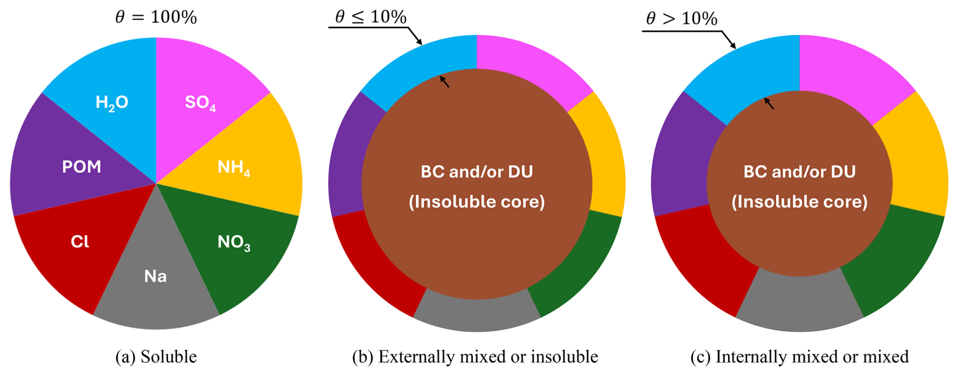
Figure 4 The three aerosol mixing states according to MADE3. (a) Soluble state, where each of the seven colors represents a soluble species, (b) externally mixed or “insoluble” state where the total soluble mass fraction θ is at most 10 % and (c) internally mixed or simply “mixed” state where the total soluble mass fraction θ is above 10 %. BC and DU denote the insoluble black carbon or mineral dust core, respectively. Figure is inspired by Kaiser et al. (2014).

The MADE3 submodel calculates tracer tendencies for both mass and particle number mixing ratios across these nine modes and nine species. These tendencies encompass several microphysical processes: gas-particle partitioning (subscript “gtp”), condensation (subscript “cond”), nucleation (subscript “nucl”), coagulation (subscript “coag”), particle growth (subscript “gr”) and aging (subscript “ag”). The general form of the governing differential equations for the mass mixing ratios C_I,M of an aerosol species I in mode M is therefore given by Eq. (2) (Aquila et al., 2011):

$$\begin{array}{}\text{(2)}& \begin{array}{rl}{\displaystyle \frac{\partial C_{I,M}}{\partial t}}& =R\left(C_{I,M}\right)+{\left.{\displaystyle \frac{\partial C_{I,M}}{\partial t}}\right|}_{\mathrm{gtp}}+{\left.{\displaystyle \frac{\partial C_{I,M}}{\partial t}}\right|}_{\mathrm{cond}}\\ & +{\left.{\displaystyle \frac{\partial C_{I,M}}{\partial t}}\right|}_{\mathrm{nucl}}+{\left.{\displaystyle \frac{\partial C_{I,M}}{\partial t}}\right|}_{\mathrm{coag}}+{\left.{\displaystyle \frac{\partial C_{I,M}}{\partial t}}\right|}_{\mathrm{gr}}\\ & +{\left.{\displaystyle \frac{\partial C_{I,M}}{\partial t}}\right|}_{\mathrm{ag}}.\end{array}\end{array}$$

The term R(C_I,M) indicates the variation of the aerosol mass mixing ratio because of removal (e.g. dry and wet deposition) and transport phenomena like convection, advection or turbulent mixing processes that are all handled outside of MADE3 by other submodels. These include sedimentation (handled by the SEDI submodel), dry deposition (handled by the DDEP submodel), wet deposition (handled by the SCAV submodel) as well as mixing from atmospheric turbulence (handled in Eulerian representation by the submodel E5VDIFF (Supplement of Emmerichs et al., 2021) and in Lagrangian representation by the submodel LGTMIX (Brinkop and Jöckel, 2019)).

The focus of this study is on aerosols containing SO₄ (I=SO₄) and their nine modes, for which the following simplifications may be applied to Eq. (2):

1. ${\left.\frac{\partial C_{{\mathrm{SO}}_{\mathrm{4}},M}}{\partial t}\right|}_{\mathrm{gtp}}=\mathrm{0}.$ The gas-particle partitioning term is neglected for SO₄, as it is assumed that H₂SO₄ has an equilibrium vapor pressure that is low enough so that it is fully transferred from the gas to the aerosol phase at each time step. The reverse conversion is also not possible, i.e., H₂SO₄ cannot re-evaporate (Kaiser et al., 2014). In MADE3, the condensation of H₂SO₄ is fully accounted for by the “cond” term.

2. ${\left.\frac{\partial C_{{\mathrm{SO}}_{\mathrm{4}},M\ne \mathrm{ks}}}{\partial t}\right|}_{\mathrm{nucl}}=\mathrm{0}.$ The nucleation term for SO₄ applies exclusively to the mass mixing ratio of the soluble Aitken mode (M=ks) as freshly formed particles via the binary homogeneous nucleation between H₂SO₄ and H₂O are assumed to instantaneously produce soluble SO₄ aerosols in the Aitken mode size range (Aquila et al., 2011; Kaiser et al., 2014; Kaiser et al., 2019).

3. ${\left.\frac{\partial C_{{\mathrm{SO}}_{\mathrm{4}},M=\mathit{\{}\mathrm{ks},\mathrm{as},\mathrm{cs}\mathit{\}}}}{\partial t}\right|}_{\mathrm{ag}}=\mathrm{0}.$ The aging process changes aerosols from the insoluble to the mixed modes when their soluble mass fractions exceed a critical threshold of 10 %. Experimental studies (Weingartner et al., 1997; Khalizov et al., 2009) have shown that aerosols with soluble mass fractions above this threshold will exhibit hygroscopic growth and expand by H₂O uptake (Aquila et al., 2011). Consequently, the aging tendency only influences the insoluble and mixed modes.

By applying these three assumptions to Eq. (2), we derive the nine differential equations for the mass mixing ratio of each SO₄ aerosol mode (Eq. 3). Each term is explained in greater detail in the coming sections.

$$\begin{array}{}\text{(3)}& \begin{array}{rl}& {\displaystyle \frac{\partial C_{{\mathrm{SO}}_{\mathrm{4}},M}}{\partial t}}=\\ & \left\{\begin{array}{l}R\left(C_{{\mathrm{SO}}_{\mathrm{4}},M}\right)+{\left.\frac{\partial C_{{\mathrm{SO}}_{\mathrm{4}},M}}{\partial t}\right|}_{\mathrm{cond}}+{\left.\frac{\partial C_{{\mathrm{SO}}_{\mathrm{4}},M}}{\partial t}\right|}_{\mathrm{nucl}}\\ +{\left.\frac{\partial C_{{\mathrm{SO}}_{\mathrm{4}},M}}{\partial t}\right|}_{\mathrm{coag}}+{\left.\frac{\partial C_{{\mathrm{SO}}_{\mathrm{4}},M}}{\partial t}\right|}_{\mathrm{gr}};M\equiv \mathrm{ks}\\ R\left(C_{{\mathrm{SO}}_{\mathrm{4}},M}\right)+{\left.\frac{\partial C_{{\mathrm{SO}}_{\mathrm{4}},M}}{\partial t}\right|}_{\mathrm{cond}}+{\left.\frac{\partial C_{{\mathrm{SO}}_{\mathrm{4}},M}}{\partial t}\right|}_{\mathrm{coag}}\\ +{\left.\frac{\partial C_{{\mathrm{SO}}_{\mathrm{4}},M}}{\partial t}\right|}_{\mathrm{gr}}+{\left.\frac{\partial C_{{\mathrm{SO}}_{\mathrm{4}},M}}{\partial t}\right|}_{\mathrm{ag}};M\equiv \mathrm{ki},\mathrm{km},\mathrm{ai},\mathrm{am},\mathrm{ci},\mathrm{cm}\\ R\left(C_{{\mathrm{SO}}_{\mathrm{4}},M}\right)+{\left.\frac{\partial C_{{\mathrm{SO}}_{\mathrm{4}},M}}{\partial t}\right|}_{\mathrm{cond}}\\ +{\left.\frac{\partial C_{{\mathrm{SO}}_{\mathrm{4}},M}}{\partial t}\right|}_{\mathrm{coag}}+{\left.\frac{\partial C_{{\mathrm{SO}}_{\mathrm{4}},M}}{\partial t}\right|}_{\mathrm{gr}};M\equiv \mathrm{as},\mathrm{cs}\end{array}\right.\end{array}\end{array}$$

2.3.1 The nucleation tendency

Homogeneous nucleation between H₂SO₄ and H₂O is a critical process behind the formation of SO₄ aerosols in the atmosphere and is calculated in MADE3 by means of a parameterization by Vehkamäki et al. (2002) for the nucleation rate J. The parameterization of J is applicable for atmospheric temperatures T between 230.15 and 305.15 K (typical of the troposphere and stratosphere), relative humidities (RH) from 0.01 % and 100 % and sulfuric acid concentrations ($C_{{\mathrm{H}}_{\mathrm{2}}{\mathrm{SO}}_{\mathrm{4}}}$) between 10⁴ and 10¹¹ molecules cm⁻³. In an earlier version of MADE3 (version 2.0b; Kaiser et al., 2014), it was assumed that the newly nucleated sulfate particles were all characterized by a representative wet diameter of 3.5 nm, although in reality they are likely to be smaller and grow to more comparable sizes via other processes like coagulation and condensation, as is acknowledged by Binkowski and Roselle (2003). In the more recent MADE3 release (version 3.0; Kaiser et al., 2019), freshly formed particles are considered to have a dry diameter of 10 nm to implicitly account for the rapid growth to larger sizes within a few hours, a phenomenon that cannot yet be resolved by global models. Compared to tropospheric observations of nucleated particles gathered by other studies (Modini et al., 2009; Ueda et al., 2016), such a modification appears to yield more accurate simulation results for the size distribution of aerosol particles and their particle number concentrations. The calculation of the SO₄ nucleation tendency follows Eq. (4):

$$\begin{array}{}\text{(4)}& \begin{array}{rl}{\left.{\displaystyle \frac{\partial C_{{\mathrm{SO}}_{\mathrm{4}},\mathrm{ks}}}{\partial t}}\right|}_{\mathrm{nucl}}& =J\left(T,\mathrm{RH},C_{{\mathrm{H}}_{\mathrm{2}}{\mathrm{SO}}_{\mathrm{4}}}\right)\times m_{\mathrm{10}\mathrm{nm}}\left(\mathrm{RH}\right)\\ & \times \exp \left[{\displaystyle \frac{\mathrm{9}}{\mathrm{2}}}{\ln }^{\mathrm{2}}{\mathit{\sigma }}_{\mathrm{ks}}\right].\end{array}\end{array}$$

The term m_10 nm(RH) denotes the mass of a freshly nucleated spherical SO₄ particle with a dry diameter of 10 nm, which depends on the ambient RH. The factor $\exp \left[\frac{\mathrm{9}}{\mathrm{2}}{\ln }^{\mathrm{2}}{\mathit{\sigma }}_{\mathrm{ks}}\right]$ relates to the geometric standard deviation of the soluble Aitken mode (σ_ks) for a lognormal distribution (see explanation of Eq. 1a). It is worth highlighting that nucleation involves only the amount of H₂SO₄ that has not yet been consumed by condensation. In reality, both processes simultaneously compete for H₂SO₄, but within MADE3, the condensation process has been set to occur before nucleation, being the slower one. This consequently amplifies the influence of SO₄ nucleation at locations where condensational sinks for H₂SO₄ are low (Kaiser et al., 2014).

2.3.2 The condensation tendency

The condensation of H₂SO₄ onto pre-existing particles leads to an overall gain in the mass mixing ratio of SO₄. As was mentioned, it is assumed that all sulfuric acid is converted from the gas to the aerosol phase and that no re-evaporation occurs in the opposite direction (Kaiser et al., 2014). This SO₄ gain (${\left.\frac{\partial C_{{\mathrm{SO}}_{\mathrm{4}},M}}{\partial t}\right|}_{\mathrm{cond}}$) is quantified by Eq. (5) and may be expressed in terms of the dimensionless coefficients ${\mathrm{\Omega }}_{{\mathrm{SO}}_{\mathrm{4}},M}$ and the amount of condensed H₂SO₄, represented by ${\left.\mathrm{\Delta }{\mathrm{H}}_{\mathrm{2}}{\mathrm{SO}}_{\mathrm{4}}\right|}_{\mathrm{cond}}$, for each aerosol mode M (Whitby et al., 1991; Aquila et al., 2011):

$$\begin{array}{}\text{(5)}& {\left.{\displaystyle \frac{\partial C_{{\mathrm{SO}}_{\mathrm{4}},M}}{\partial t}}\right|}_{\mathrm{cond}}={\mathrm{\Omega }}_{{\mathrm{SO}}_{\mathrm{4}},M}\times {\displaystyle \frac{{\left.\mathrm{\Delta }{\mathrm{H}}_{\mathrm{2}}{\mathrm{SO}}_{\mathrm{4}}\right|}_{\mathrm{cond}}}{\mathrm{\Delta }t}}.\end{array}$$

The coefficients ${\mathrm{\Omega }}_{{\mathrm{SO}}_{\mathrm{4}},M}$ measure the modal contribution of the SO₄ growth term for mode M ($G_{{\mathrm{SO}}_{\mathrm{4}},M}^{\left(\mathrm{3}\right)}$), which is proportional to the time rate of change of the total volume of aerosol particles in a specific mode M, relative to the sum of all nine modal growth terms, as expressed by Eq. (5a). The variable ${\left.\mathrm{\Delta }{\mathrm{H}}_{\mathrm{2}}{\mathrm{SO}}_{\mathrm{4}}\right|}_{\mathrm{cond}}$ is calculated by solving a first-order linear differential equation (Eq. 5b) that describes the difference between the gas-phase production rate of sulfuric acid (P) and its condensational loss rate L (Aquila et al., 2011; Kaiser et al., 2014):

$$\begin{array}{}\text{(5a)}& {\displaystyle }{\mathrm{\Omega }}_{{\mathrm{SO}}_{\mathrm{4}},M}={\displaystyle \frac{G_{{\mathrm{SO}}_{\mathrm{4}},M}^{\left(\mathrm{3}\right)}}{\sum _{j=\mathrm{1}}^{\mathrm{9}}{G}_{{\mathrm{SO}}_{\mathrm{4}},j}^{\left(\mathrm{3}\right)}}},\text{(5b)}& {\displaystyle \frac{\mathrm{d}{C}_{{\mathrm{H}}_{\mathrm{2}}{\mathrm{SO}}_{\mathrm{4}}}\left(\mathrm{t}\right)}{\mathrm{d}t}}=P-L\cdot C_{{\mathrm{H}}_{\mathrm{2}}{\mathrm{SO}}_{\mathrm{4}}}\left(\mathrm{t}\right).\end{array}$$

The growth rates G featured in Eq. (5a) may be computed by finding the harmonic mean of the growth rates for the SO₄ aerosol in mode M for two regimes: the free-molecular regime in which collisions between gas molecules are not as frequent and the near-continuum regime in which collisions are frequent enough for the gas to be considered a continuous fluid. Other variables like the saturation vapor pressure and diffusion coefficients of sulfuric acid are also necessary to calculate ${\mathrm{\Omega }}_{{\mathrm{SO}}_{\mathrm{4}},M}$. Further details on the calculation of the terms in Eq. (5) are provided by Aquila et al. (2011) and Kaiser et al. (2014).

2.3.3 The coagulation tendency

Two types of coagulation processes are distinguished: intra- and intermodal. The former occurs between particles of the same mode and produces aerosols that remain in that mode. The latter occurs between particles from different size and mixing states and results in particles with diameters comparable to the larger of the colliding aerosols. Only intermodal coagulation is therefore relevant for the spatio-temporal evolution of aerosol mass mixing ratios. The contribution to mode M of SO₄ resulting from the coagulation of an aerosol in mode p and another in mode q is given by Eq. (6) (Kaiser et al., 2014):

$$\begin{array}{}\text{(6)}& \begin{array}{rl}& {\left.{\displaystyle \frac{\partial C_{{\mathrm{SO}}_{\mathrm{4}},M}}{\partial t}}\right|}_{\mathrm{coag}}={\displaystyle \frac{\mathit{\pi }}{\mathrm{6}}}\sum _{p=\mathrm{1}}^{\mathrm{9}}\sum _{q=\mathrm{1}}^{\mathrm{9}}[\left({\mathit{\delta }}_{M,{\mathit{\tau }}_{pq}}-{\mathit{\delta }}_{M,p}\right)\\ & \cdot {\displaystyle \frac{C_{{\mathrm{SO}}_{\mathrm{4}},p}}{{\sum }_{s=\mathrm{1}}^A{C}_{\mathrm{s},p}}}\cdot {\mathit{\rho }}_p\underset{\mathrm{0}}{\overset{\mathrm{\infty }}{\int }}\underset{\mathrm{0}}{\overset{\mathrm{\infty }}{\int }}{\left(D_{\mathrm{1}}\right)}^{\mathrm{3}}\mathit{\beta }\left(D_{\mathrm{1}},D_{\mathrm{2}}\right)n_p\left(D_{\mathrm{1}}\right)\\ & n_q\left(D_{\mathrm{2}}\right)\mathrm{d}{D}_{\mathrm{1}}\mathrm{d}{D}_{\mathrm{2}}+\left({\mathit{\delta }}_{M,{\mathit{\tau }}_{pq}}-{\mathit{\delta }}_{M,q}\right)\cdot {\displaystyle \frac{C_{{\mathrm{SO}}_{\mathrm{4}},q}}{{\sum }_{s=\mathrm{1}}^A{C}_{\mathrm{s},q}}}\\ & \cdot {\mathit{\rho }}_q\underset{\mathrm{0}}{\overset{\mathrm{\infty }}{\int }}\underset{\mathrm{0}}{\overset{\mathrm{\infty }}{\int }}{\left(D_{\mathrm{2}}\right)}^{\mathrm{3}}\mathit{\beta }\left(D_{\mathrm{1}},D_{\mathrm{2}}\right)n_p\left(D_{\mathrm{1}}\right)n_q\left(D_{\mathrm{2}}\right)\mathrm{d}{D}_{\mathrm{1}}\mathrm{d}{D}_{\mathrm{2}}].\end{array}\end{array}$$

The resulting mode for each type of collision in MADE3 is governed by a categorical variable τ_pq where p and q are the colliding modes. The possible values of τ_pq are detailed in Table 2 from Kaiser et al. (2014), having also a dependency on the particle's soluble mass fraction θ relative to water. The symbol δ_x,y denotes the Kronecker delta, which assumes a unit value only when both subscripts x and y refer to the same aerosol mode and being zero otherwise. The mass mixing ratios of SO₄ corresponding to modes p and q are indicated by $C_{{\mathrm{SO}}_{\mathrm{4}},p}$ and $C_{{\mathrm{SO}}_{\mathrm{4}},q}$ and their densities by ρ_p and ρ_q respectively. The upper bound A of the summations indicates the total number of tracer species s in MADE3, i.e., SO₄, NH₄, NO₃, Na, Cl, POM, BC, DU and H₂O. The particle number distribution for modes p and q with particle diameters D₁ and D₂, are written as n_p(D₁) and n_q(D₂), respectively. Lastly, the Brownian coagulation kernels for particles with diameters D₁ and D₂ are expressed as β(D₁,D₂), which vary according to the aerosol flow regime, i.e., free-molecular or near-continuum, as well as on the ambient temperature, pressure and dynamic viscosity. From a more intuitive perspective, they describe the probability of collision between particles of diameters D₁ and D₂ according to Brownian motion. Their complete mathematical formulations are described by Eq. (C17) in Appendix C.

2.3.4 The growth and aging tendency

Although in theory the growth and aging processes are distinct, as in Eq. (2), they are coupled and therefore not given each their own tendency in MADE3. The collective tendency in MADE3 that describes growth and aging is called “rename” and is impacted by both, the condensation and the coagulation processes. The growth process, for instance, refers to the possibility of aerosols growing as they either coagulate or condense onto other pre-existing particles. This may lead to a redistribution in the aerosol modes as particles grow and are reclassified from the Aitken to the accumulation mode. The aging process, in turn, relates to the transformation of insoluble particles via the acquisition of a soluble coating that alters their mixing state from hydrophobic to hydrophilic. By default, if the soluble mass fraction of an insoluble mode reaches a threshold of 10 %, the mode is turned to a mixed mode. Aging therefore only impacts the insoluble and mixed modes of SO₄ (Aquila et al., 2011; Kaiser et al., 2014).

2.4 The aerosol removal and transport processes

The removal processes included in the term $R\left(C_{{\mathrm{SO}}_{\mathrm{4}},M}\right)$ of Eq. (3) are dry deposition, sedimentation and scavenging of aerosols. Dry deposition refers to the removal of atmospheric aerosols through various interactions with surfaces, such as land or sea, and includes mechanisms such as impaction, interception and diffusion (Farmer et al., 2021). Although sedimentation is a subset of dry deposition, there are two notable differences between them in the coding of each process.

Firstly, sedimentation is handled by the SEDI submodel (Kerkweg et al., 2006a) and applies to the entirety of the simulation's vertical domain, whereas dry deposition, handled by the DDEP submodel (Kerkweg et al., 2006a), only applies to the lowermost layer of the model. Secondly, sedimentation solely affects the removal of aerosols and not of gaseous species due to mass considerations.

The dry deposition flux for aerosols is proportional to the dry deposition velocity v_d, which can vary according to the surface type: vegetation (subscript “veg”), soil and snow (subscript “slsn”) and water (subscript “wat”). The dry deposition tendency for the SO₄ aerosol is represented by Eq. (7), where parameters β₁, β₂ and β₃ depend on the surface type:

$$\begin{array}{}\text{(7)}& \begin{array}{rl}& {\left.{\displaystyle \frac{\partial C_{{\mathrm{SO}}_{\mathrm{4}},M}}{\partial t}}\right|}_{\mathrm{DDEP}}\propto \\ & \underset{v_{\mathrm{d}}}{\underbrace{{\mathit{\beta }}_{\mathrm{1}}\cdot v_{\mathrm{d},\mathrm{veg}}\left({\mathrm{SO}}_{\mathrm{4}}\right)+{\mathit{\beta }}_{\mathrm{2}}\cdot v_{\mathrm{d},\mathrm{slsn}}\left({\mathrm{SO}}_{\mathrm{4}}\right)+{\mathit{\beta }}_{\mathrm{3}}\cdot v_{\mathrm{d},\mathrm{wat}}\left({\mathrm{SO}}_{\mathrm{4}}\right)}}.\end{array}\end{array}$$

The sedimentation tendency (Eq. 8) is in turn proportional to the terminal sedimentation velocity v_t, which depends on the Stokes velocity v_Stokes, the Cunningham slip flow correction factor (f_csf) and the Slinn factor (f_s). The latter is used to correct for the larger average sedimentation velocity of a lognormal population of aerosols when compared to the sedimentation velocity of a particle with an average particle diameter:

$$\begin{array}{}\text{(8)}& {\left.{\displaystyle \frac{\partial C_{{\mathrm{SO}}_{\mathrm{4}},M}}{\partial t}}\right|}_{\mathrm{SEDI}}\propto \underset{v_{\mathrm{t}}}{\underbrace{v_{\mathrm{Stokes}}\left(M\right)\cdot f_{\mathrm{csf}}\left(M\right)\cdot f_{\mathrm{s}}\left(M\right)}}.\end{array}$$

The expressions for the terms needed to compute both dry deposition and sedimentation velocities in Eqs. (7) and (8), are documented by Kerkweg et al. (2006a).

Wet deposition of SO₄ refers to scavenging because of the precipitation of either ice or liquid water. Aerosol lifetimes are therefore strongly influenced by the interaction between wet and dry deposition processes. Global studies have shown that wet deposition is more important for removing aerosols, but dry deposition is naturally dominant in cloud-free regions where precipitation is unlikely (Farmer et al., 2021). Wet deposition is calculated by the SCAV submodel (Tost et al., 2006) and considers two mechanisms: nucleation scavenging (rainout) and impaction scavenging (washout). The former involves the removal of chemical species from the atmosphere by means of nucleation and subsequent growth of cloud droplets that dissolve them and are then rained out. The latter process refers to the removal of aerosols and gases via their direct collision with raindrops. In a cloud-free region, nucleation scavenging is disregarded and only impaction scavenging is considered. Both mechanisms are contemplated via parameterizations that depend on, e.g., the Brownian motion of aerosols. These are described in further detail by Tost et al. (2006).

The transport of SO₄ in a Lagrangian framework is made possible primarily by three submodels: ATTILA, LGTMIX and TREXP. The Atmospheric Tracer Transport in a LAgrangian (ATTILA; Reithmeier and Sausen, 2002; Brinkop and Jöckel, 2019) submodel is the transport scheme for the Lagrangian air parcels and it resolves their advection according to the EMAC wind field and their convective motion. The LaGrangian Tracer MIXing (LGTMIX; Brinkop and Jöckel, 2019) submodel estimates the mass exchange of different chemical species from the isotropic mixing that occurs from atmospheric turbulence. Lastly, although the Tracer Release Experiments from Point sources (TREXP; Jöckel et al., 2010) submodel is not directly involved in the transport of tracers, it assists ATTILA and LGTMIX by defining the initial emission conditions (i.e. position, time and amount emitted) for point sources.

3 The new AIRTRAC v2.0 submodel

The AIRTRAC submodel (Supplement of Grewe et al., 2014a) was originally developed to improve our understanding of some of aviation's gas-phase emissions, more specifically that of NO_x and H₂O. The new AIRTRAC v2.0 submodel now has expanded capabilities to calculate the contributions of aircraft H₂SO₄ and SO₂ emissions to the nine aerosol modes of SO₄. As in the gas-phase scheme, source contributions are computed using the tagging approach of Grewe (2013), which is shown in Eq. (9), and the method applied by Itahashi et al. (2017) and Wu et al. (2017) (hereafter IW17). In IW17, SO₄ microphysical processes (e.g. coagulation and condensation) are scaled according to precursor emissions such as SO₂, while removal processes (dry and wet deposition) are scaled relative to the remaining aviation-attributable SO₄. State variables, like the different aerosol modes of SO₄, are denoted by x_M, where x specifies the chemical species and M the mode. The index j refers to the number of tagging categories that together add up to the quantity x_M. The term $P_M^j\left(\mathrm{t}\right)$ indicates the time-dependent contribution of tagging category j to mode M and F_M is the state-dependent forcing for mode M, which could represent production and/or loss terms associated with a state variable x_M.

$$\begin{array}{}\text{(9)}& {\displaystyle \frac{\partial }{\partial t}}{x}_M^j=P_M^j\left(t\right)+F_M\left(\mathit{x}\right){\displaystyle \frac{{\mathit{x}}^{j^{\mathrm{T}}}\mathrm{\nabla }{F}_M\left(\mathit{x}\right)}{{\mathit{x}}^{\mathrm{T}}\cdot \mathrm{\nabla }{F}_M\left(\mathit{x}\right)}}\end{array}$$

This approach entails the calculation of a fractional weight, $\frac{{\mathit{x}}^{j^T}\mathrm{\nabla }{F}_M\left(\mathit{x}\right)}{{\mathit{x}}^{\mathrm{T}}\cdot \mathrm{\nabla }{F}_M\left(\mathit{x}\right)}$, that scales the total forcing term F_M(x) to isolate the forcing component attributable to tagging category j for mode M. The numerator represents the weighted influence of tagging category j on the total forcing F_M while the denominator is the total forcing from all categories. This approach ensures that the sum of the tagged contributions $x_M^j$ from all categories equals the solution of the original ordinary differential equation (ODE) for the untagged total x_M (Grewe, 2013). In the context of this study, two tagging categories are distinguished: aviation (index “avi”) and the remaining sources (index “rem”), which include anthropogenic activity, other transport sectors like shipping and biogenic emissions. This fraction is applied to the MADE3 tendencies, allowing the model to calculate aviation-attributable contributions to SO₄ enhancement. By construction, this guarantees a closed budget for the total amount of SO₄ in the atmosphere, as the sum of the individual sources mathematically equates to the total (Eq. 10).

$$\begin{array}{}\text{(10)}& {\displaystyle \frac{\partial C_{{\mathrm{SO}}_{\mathrm{4}},M}}{\partial t}}={\left.{\displaystyle \frac{\partial C_{{\mathrm{SO}}_{\mathrm{4}},M}}{\partial t}}\right|}^{\mathrm{avi}}+{\left.{\displaystyle \frac{\partial C_{{\mathrm{SO}}_{\mathrm{4}},M}}{\partial t}}\right|}^{\mathrm{rem}}\end{array}$$

3.1 Submodel infrastructure

AIRTRAC v2.0 leverages the same technical infrastructure of its predecessor, introducing new Lagrangian tracers dedicated to SO₄, SO₂ and H₂SO₄ chemistry. Some of these include tracers specific to individual aerosol microphysical processes such as coagulation, enabling the estimation of each process's influence on an aerosol mode. A new subroutine called “airtrac_aerosol_integrate” was created to handle the calculation of aerosol chemistry along the Lagrangian air parcel trajectories. The AIRTRAC control (CTRL) and coupling (CPL) namelists have also been adapted to now allow the user to select the value of “airtrac_mode”, which should be set to “1” when studying SO₄ aerosols and to “2” for the gas-phase analysis mode.

3.2 Tracking aviation SO₂ and H₂SO₄ emissions

As SO₂ and H₂SO₄ are both precursors of SO₄ and are directly emitted by aircraft, their evolution throughout the course of a simulation must be tracked to properly account for aviation's impact on sulfate. The key gas-phase, tropospheric reaction involving SO₂ that leads to the production of H₂SO₄ in the chemistry mechanism adopted in this study is represented by the net Reaction (R4):

$$\begin{array}{}\text{(R4)}& {\mathrm{SO}}_{\mathrm{2}}+\mathrm{OH}\to {\mathrm{H}}_{\mathrm{2}}{\mathrm{SO}}_{\mathrm{4}}+{\mathrm{HO}}_{\mathrm{2}}.\end{array}$$

The evolution of aviation SO₂ is simplified and described in AIRTRAC as a pure loss process, where it is oxidized to form H₂SO₄ according to Reaction (R4). While processes such as scavenging contribute to SO₂ removal, these are excluded from the analysis due to the computational constraints arising from the difficulty of storing all the liquid-phase tracers associated with the production of SO₄ from SO₂ (Tost et al., 2006). These removal processes primarily affect liquid-phase species anyway and thus have a smaller impact on the simulated gas-phase SO₂. Consequently, the mixing ratio of aviation-attributable SO₂ (${\left.C_{{\mathrm{SO}}_{\mathrm{2}}}\right|}^{\mathrm{avi}}$), is based on the initial amount emitted into the atmosphere ($C_{{\mathrm{SO}}_{\mathrm{2}}}\left(t=\mathrm{0}\right))$ and the production rate of H₂SO₄ from SO₂ that is provided by the MECCA submodel (${\mathrm{P}}_{{\mathrm{H}}_{\mathrm{2}}{\mathrm{SO}}_{\mathrm{4}}}$), as is illustrated by Eq. (11). Unlike in Eq. (3), the term $R\left(C_{{\mathrm{SO}}_{\mathrm{2}}}\right)$ only contemplates the effects of isotropic turbulent mixing:

$$\begin{array}{}\text{(11)}& \begin{array}{rl}{\left.C_{{\mathrm{SO}}_{\mathrm{2}}}\right|}^{\mathrm{avi}}& =\underset{\text{Emission}}{\underbrace{C_{{\mathrm{SO}}_{\mathrm{2}}}(t=\mathrm{0})}}-\underset{\text{Tagging ratio}}{\underbrace{{\displaystyle \frac{C_{{\mathrm{SO}}_{\mathrm{2}}}{|}^{\mathrm{avi}}}{C_{{\mathrm{SO}}_{\mathrm{2}}}{|}^{\mathrm{avi}}+C_{{\mathrm{SO}}_{\mathrm{2}}}{|}^{\mathrm{rem}}}}}}\\ & \times \underset{\text{Molar masses}}{\underbrace{{\displaystyle \frac{M_{{\mathrm{SO}}_{\mathrm{2}}}}{M_{{\mathrm{H}}_{\mathrm{2}}{\mathrm{SO}}_{\mathrm{4}}}}}}}\times \underset{\text{Production rate}}{\underbrace{P_{{\mathrm{H}}_{\mathrm{2}}{\mathrm{SO}}_{\mathrm{4}}}}}\times \mathrm{\Delta }t+\underset{\text{Turbulence}}{\underbrace{R\left(C_{{\mathrm{SO}}_{\mathrm{2}}}\right)}}.\end{array}\end{array}$$

In theory, the tagging ratio that scales the aviation-attributable SO₂ in Eq. (11) should consider the amount of OH emanating from both, aviation and other sources, and therefore be expressed as $\frac{\mathrm{1}}{\mathrm{2}}\times \left(\frac{{\left.C_{{\mathrm{SO}}_{\mathrm{2}}}\right|}^{\mathrm{avi}}}{{\left.C_{{\mathrm{SO}}_{\mathrm{2}}}\right|}^{\mathrm{avi}}+{\left.C_{{\mathrm{SO}}_{\mathrm{2}}}\right|}^{\mathrm{rem}}}+\frac{{\left.C_{\mathrm{OH}}\right|}^{\mathrm{avi}}}{{\left.C_{\mathrm{OH}}\right|}^{\mathrm{avi}}+{\left.C_{\mathrm{OH}}\right|}^{\mathrm{rem}}}\right)$, corresponding to the case of bimolecular reactions by Grewe et al. (2010) and Grewe (2013). However, this contribution is omitted in Eq. (11), as this study focuses exclusively on the influence of aviation SO₂ and H₂SO₄ emissions on SO₄. Since OH is not directly emitted by aircraft, fully tracking it would at least require other gas-phase aircraft emissions like NO_x and CO and their chemical cycling in the atmosphere with other compounds like HO₂ and O₃ to be completely followed, which is beyond the scope of this assessment. Lastly, as the production rate ${\mathrm{P}}_{{\mathrm{H}}_{\mathrm{2}}{\mathrm{SO}}_{\mathrm{4}}}$ is the amount of H₂SO₄ produced from the oxidation of SO₂, it must be converted into the equivalent amount of SO₂ loss by multiplying it by the ratio of molar masses ($\frac{M_{{\mathrm{SO}}_{\mathrm{2}}}}{M_{{\mathrm{H}}_{\mathrm{2}}{\mathrm{SO}}_{\mathrm{4}}}}$).

To track the evolution of gas-phase, aviation-attributable H₂SO₄, the amount produced from the conversion of SO₂ described in Eq. (11) must be considered along with two primary sinks: the binary nucleation of H₂SO₄ with H₂O and the condensation of H₂SO₄ onto pre-existing particles, as is represented in Eq. (12). As a limitation to the approach represented by Eqs. (11) and (12), only the gas-phase formation of H₂SO₄ (produced from the hydrolysis of SO₃ via Reactions R1–R3) is considered in our analysis. The liquid-phase production that involves the oxidation by O₃ and hydrogen peroxide (H₂O₂) of H₂SO₃, which in turn is formed by the hydrolysis of SO₂ (Sheng et al., 2018; Shostak et al., 2019), is excluded. While this pathway is the dominant source of sulfuric acid (Textor et al., 2006), incorporating it is challenging, due to the cloud evaporation assumption described by Tost et al. (2006), which considers that clouds and aqueous-phase species are fully evaporated at the end of each time step. This assumption is used to avoid the high computation and memory costs that would otherwise be required to advect both gas- and aqueous-phase tracer species. The term $R\left(C_{{\mathrm{H}}_{\mathrm{2}}{\mathrm{SO}}_{\mathrm{4}}}\right)$ therefore again only represents isotropic turbulent mixing.

$$\begin{array}{}\text{(12)}& \begin{array}{rl}& {\left.C_{{\mathrm{H}}_{\mathrm{2}}{\mathrm{SO}}_{\mathrm{4}}}\right|}^{\mathrm{avi}}=\underset{\text{Emission}}{\underbrace{C_{{\mathrm{H}}_{\mathrm{2}}{\mathrm{SO}}_{\mathrm{4}}}(t=\mathrm{0})}}\\ & +\underset{\mathrm{Oxidation}\mathrm{of}{\mathrm{SO}}_{\mathrm{2}}}{\underbrace{{\displaystyle \frac{C_{{\mathrm{SO}}_{\mathrm{2}}}{|}^{\mathrm{avi}}}{C_{{\mathrm{SO}}_{\mathrm{2}}}{|}^{\mathrm{avi}}+C_{{\mathrm{SO}}_{\mathrm{2}}}{|}^{\mathrm{rem}}}}\times P_{{\mathrm{H}}_{\mathrm{2}}{\mathrm{SO}}_{\mathrm{4}}}\times \mathrm{\Delta }t}}+\mathrm{\dots }\\ & \mathrm{\dots }-\underset{\mathrm{Nucleation}\mathrm{of}{\mathrm{H}}_{\mathrm{2}}{\mathrm{SO}}_{\mathrm{4}}}{\underbrace{{\displaystyle \frac{C_{{\mathrm{H}}_{\mathrm{2}}{\mathrm{SO}}_{\mathrm{4}}}{|}^{\mathrm{avi}}}{C_{{\mathrm{H}}_{\mathrm{2}}{\mathrm{SO}}_{\mathrm{4}}}{|}^{\mathrm{avi}}+C_{{\mathrm{H}}_{\mathrm{2}}{\mathrm{SO}}_{\mathrm{4}}}{|}^{\mathrm{rem}}}}\times {\displaystyle \frac{\partial C_{{\mathrm{H}}_{\mathrm{2}}{\mathrm{SO}}_{\mathrm{4}}}}{\partial t}}{|}_{\mathrm{nucl}}^{\mathrm{avi}}\times \mathrm{\Delta }t}}+\mathrm{\dots }\\ & \mathrm{\dots }-\underset{\mathrm{Condensation}\mathrm{of}{\mathrm{H}}_{\mathrm{2}}{\mathrm{SO}}_{\mathrm{4}}}{\underbrace{{\displaystyle \frac{C_{{\mathrm{H}}_{\mathrm{2}}{\mathrm{SO}}_{\mathrm{4}}}{|}^{\mathrm{avi}}}{C_{{\mathrm{H}}_{\mathrm{2}}{\mathrm{SO}}_{\mathrm{4}}}{|}^{\mathrm{avi}}+C_{{\mathrm{H}}_{\mathrm{2}}{\mathrm{SO}}_{\mathrm{4}}}{|}^{\mathrm{rem}}}}\times {\displaystyle \frac{\partial C_{{\mathrm{H}}_{\mathrm{2}}{\mathrm{SO}}_{\mathrm{4}}}}{\partial t}}{|}_{\mathrm{cond}}^{\mathrm{avi}}\times \mathrm{\Delta }t}}\\ & +\underset{\mathrm{Turbulence}}{\underbrace{R\left(C_{{\mathrm{H}}_{\mathrm{2}}{\mathrm{SO}}_{\mathrm{4}}}\right)}}\end{array}\end{array}$$

3.3 Aviation's contribution to SO₄ via nucleation and condensation of H₂SO₄

The contribution from aviation to the formation of the soluble Aitken mode of SO₄ via the binary nucleation of H₂SO₄-H₂O is estimated by applying a tagging ratio to the MADE3 nucleation tendency (Eq. 4). This tagging ratio in Eq. (13) naturally involves H₂SO₄, given that sulfuric acid from aviation (${\left.C_{{\mathrm{H}}_{\mathrm{2}}{\mathrm{SO}}_{\mathrm{4}}}\right|}^{\mathrm{avi}}$) drives the nucleation process.

$$\begin{array}{}\text{(13)}& \begin{array}{rl}{\left.{\displaystyle \frac{\partial C_{{\mathrm{SO}}_{\mathrm{4}},\mathrm{ks}}}{\partial t}}\right|}_{\mathrm{nucl}}^{\mathrm{avi}}& ={\displaystyle \frac{{\left.C_{{\mathrm{H}}_{\mathrm{2}}{\mathrm{SO}}_{\mathrm{4}}}\right|}^{\mathrm{avi}}}{{\left.C_{{\mathrm{H}}_{\mathrm{2}}{\mathrm{SO}}_{\mathrm{4}}}\right|}^{\mathrm{avi}}+{\left.C_{{\mathrm{H}}_{\mathrm{2}}{\mathrm{SO}}_{\mathrm{4}}}\right|}^{\mathrm{rem}}}}\\ & \times {\left.{\displaystyle \frac{\partial C_{{\mathrm{SO}}_{\mathrm{4}},\mathrm{ks}}}{\partial t}}\right|}_{\mathrm{nucl}}\end{array}\end{array}$$

Aviation's contribution to SO₄ via the condensation of H₂SO₄ is estimated in a fashion similar to Eq. (13), as the tagging ratio is the same (Eq. 14) due to the central role of H₂SO₄ also in this process. The main difference is that the condensation process may contribute to increasing any one of the nine SO₄ aerosol modes.

$$\begin{array}{}\text{(14)}& \begin{array}{rl}{\left.{\displaystyle \frac{\partial C_{{\mathrm{SO}}_{\mathrm{4}},M}}{\partial t}}\right|}_{\mathrm{cond}}^{\mathrm{avi}}& ={\displaystyle \frac{{\left.C_{{\mathrm{H}}_{\mathrm{2}}{\mathrm{SO}}_{\mathrm{4}}}\right|}^{\mathrm{avi}}}{{\left.C_{{\mathrm{H}}_{\mathrm{2}}{\mathrm{SO}}_{\mathrm{4}}}\right|}^{\mathrm{avi}}+{\left.C_{{\mathrm{H}}_{\mathrm{2}}{\mathrm{SO}}_{\mathrm{4}}}\right|}^{\mathrm{rem}}}}\\ & \times {\left.{\displaystyle \frac{\partial C_{{\mathrm{SO}}_{\mathrm{4}},M}}{\partial t}}\right|}_{\mathrm{cond}}\end{array}\end{array}$$

3.4 Aviation's contribution to SO₄ via particle coagulation, growth and aging

We first derive an expression for aviation's contribution to the soluble Aitken mode (M=ks) of SO₄ via coagulation by applying the tagging formulation in Eq. (9). For clarity and conciseness in representing the full coagulation equation (Eq. 6), vector notation is introduced for the state variables x according to Eq. (15) for all nine aerosol modes, where x₁, for instance, is the mass concentration of mode “ks”, i.e., $x_{\mathrm{1}}\equiv C_{{\mathrm{SO}}_{\mathrm{4}},\mathrm{ks}}$. Each state variable x_i represents the sum of contributions from all sources, in this study the sources are $j=\left\{\mathrm{avi},\mathrm{rem}\right\}$.

$$\begin{array}{}\text{(15)}& \mathit{x}=\left[\begin{array}{l}{x}_{\mathrm{1}}\\ x_{\mathrm{2}}\\ x_{\mathrm{3}}\\ x_{\mathrm{4}}\\ x_{\mathrm{5}}\\ x_{\mathrm{6}}\\ x_{\mathrm{7}}\\ x_{\mathrm{8}}\\ x_{\mathrm{9}}\end{array}\right]=\left[\begin{array}{l}{x}_{\mathrm{1}}^{\mathrm{avi}}+x_{\mathrm{1}}^{\mathrm{rem}}\\ x_{\mathrm{2}}^{\mathrm{avi}}+x_{\mathrm{2}}^{\mathrm{rem}}\\ x_{\mathrm{3}}^{\mathrm{avi}}+x_{\mathrm{3}}^{\mathrm{rem}}\\ x_{\mathrm{4}}^{\mathrm{avi}}+x_{\mathrm{4}}^{\mathrm{rem}}\\ x_{\mathrm{5}}^{\mathrm{avi}}+x_{\mathrm{5}}^{\mathrm{rem}}\\ x_{\mathrm{6}}^{\mathrm{avi}}+x_{\mathrm{6}}^{\mathrm{rem}}\\ x_{\mathrm{7}}^{\mathrm{avi}}+x_{\mathrm{7}}^{\mathrm{rem}}\\ x_{\mathrm{8}}^{\mathrm{avi}}+x_{\mathrm{8}}^{\mathrm{rem}}\\ x_{\mathrm{9}}^{\mathrm{avi}}+x_{\mathrm{9}}^{\mathrm{rem}}\end{array}\right]=\left[\begin{array}{l}{C}_{{\mathrm{SO}}_{\mathrm{4}},\mathrm{ks}}\\ C_{{\mathrm{SO}}_{\mathrm{4}},\mathrm{km}}\\ C_{{\mathrm{SO}}_{\mathrm{4}},\mathrm{ki}}\\ C_{{\mathrm{SO}}_{\mathrm{4}},\mathrm{as}}\\ C_{{\mathrm{SO}}_{\mathrm{4}},\mathrm{am}}\\ C_{{\mathrm{SO}}_{\mathrm{4}},\mathrm{ai}}\\ C_{{\mathrm{SO}}_{\mathrm{4}},\mathrm{cs}}\\ C_{{\mathrm{SO}}_{\mathrm{4}},\mathrm{cm}}\\ C_{{\mathrm{SO}}_{\mathrm{4}},\mathrm{ci}}\end{array}\right]\end{array}$$

The coagulation kernels are also more compactly rewritten (Eqs. 16a and 16b), where p and q are the modes of the colliding particles. Additionally, the summation in the denominator of Eq. (6) for an aerosol in mode p with a diameter D₁ will be reformulated more succinctly as ${\sum }_{s=\mathrm{1}}^{A=\mathrm{9}}{C}_{\mathrm{s},p}=x_{\mathrm{1}}+C_p$, where $C_p=C_{{\mathrm{NH}}_{\mathrm{4}},p}+C_{{\mathrm{NO}}_{\mathrm{3}},p}+C_{\mathrm{Na},p}+C_{\mathrm{Cl},p}+C_{\mathrm{POM},p}+C_{\mathrm{BC},p}+C_{\mathrm{DU},p}+C_{{\mathrm{H}}_{\mathrm{2}}\mathrm{O},p}$. We also note that $f_{p,q}=f_{q,p}^{\prime }$.

$$\begin{array}{}\text{(16a)}& {\displaystyle }{f}_{p,q}=\underset{\mathrm{0}}{\overset{\mathrm{\infty }}{\int }}\underset{\mathrm{0}}{\overset{\mathrm{\infty }}{\int }}{\left(D_{\mathrm{1}}\right)}^{\mathrm{3}}\mathit{\beta }\left(D_{\mathrm{1}},D_{\mathrm{2}}\right)n_p\left(D_{\mathrm{1}}\right)n_q\left(D_{\mathrm{2}}\right)\mathrm{d}{D}_{\mathrm{1}}\mathrm{d}{D}_{\mathrm{2}}\text{(16b)}& {\displaystyle }{f}_{p,q}^{\prime }=\underset{\mathrm{0}}{\overset{\mathrm{\infty }}{\int }}\underset{\mathrm{0}}{\overset{\mathrm{\infty }}{\int }}{\left(D_{\mathrm{2}}\right)}^{\mathrm{3}}\mathit{\beta }\left(D_{\mathrm{1}},D_{\mathrm{2}}\right)n_p\left(D_{\mathrm{1}}\right)n_q\left(D_{\mathrm{2}}\right)\mathrm{d}{D}_{\mathrm{1}}\mathrm{d}{D}_{\mathrm{2}}\end{array}$$

When evaluating the double summations of Eq. (6) for the case M=ks, it is worth noting that for intermodal coagulation, i.e., p≠q, the value of τ_pq≠ks. In other words, when two particles from different modes collide, the destination mode will never be the soluble Aitken mode (Table 2 from Kaiser et al., 2014). It follows that since τ_pq≠ks, the Kronecker deltas depending on τ_pq will be zero: ${\mathit{\delta }}_{\mathrm{ks},{\mathit{\tau }}_{pq}}=\mathrm{0}$. In contrast, the Kronecker deltas δ_ks,p and δ_ks,q evaluate to “1” whenever either mode p or q is also ks. We note that if p=q, the coagulation tendency is zero, as intramodal collisions do not affect mass concentrations. It is also essential to recall that the destination mode of the coagulated particle depends on the soluble mass fraction θ of the final particle. This dependency implies that the coagulation tendency for each of the nine modes will be a piecewise function (F₁) conditioned by θ. Combining Eqs. (6) and (16) leads to a more compact formulation of the coagulation tendency for mode ks (Eq. 17).

$$\begin{array}{}\text{(17)}& \begin{array}{rl}& {\left.{\displaystyle \frac{\partial x_{\mathrm{1}}}{\partial t}}\right|}_{\mathrm{coag}}=F_{\mathrm{1}}\left(\mathit{x}\right)\\ & =\left\{\begin{array}{l}-A\frac{x_{\mathrm{1}}}{x_{\mathrm{1}}+C_{\mathrm{1}}};\mathit{\theta }=\mathrm{1}\left(\mathrm{Soluble}\right)\\ -A^{\prime }\frac{x_{\mathrm{1}}}{x_{\mathrm{1}}+C_{\mathrm{1}}};\mathrm{0.1}\le \mathit{\theta }<\mathrm{1}\left(\mathrm{Mixed}\right)\\ -A^{\prime \prime }\frac{x_{\mathrm{1}}}{x_{\mathrm{1}}+C_{\mathrm{1}}};\mathrm{0}\le \mathit{\theta }<\mathrm{0.1}\left(\mathrm{Insoluble}\right)\end{array}\right.\end{array}\end{array}$$

The coefficients A, A^′ and A^′′ are defined as follows, where the subscripts refer to the colliding modes (see Eq. 15 for details):

$$\begin{array}{rl}& A={\mathit{\rho }}_{\mathrm{1}}{\displaystyle \frac{\mathit{\pi }}{\mathrm{6}}}\left[f_{\mathrm{1},\mathrm{4}}+f_{\mathrm{1},\mathrm{7}}\right]\\ & A^{\prime }={\mathit{\rho }}_{\mathrm{1}}{\displaystyle \frac{\mathit{\pi }}{\mathrm{6}}}\left[f_{\mathrm{1},\mathrm{3}}+f_{\mathrm{1},\mathrm{5}}+f_{\mathrm{1},\mathrm{6}}+f_{\mathrm{1},\mathrm{8}}+f_{\mathrm{2},\mathrm{1}}^{\prime }\right]\\ & A^{\prime \prime }={\mathit{\rho }}_{\mathrm{1}}{\displaystyle \frac{\mathit{\pi }}{\mathrm{6}}}\left[f_{\mathrm{1},\mathrm{3}}+f_{\mathrm{1},\mathrm{6}}+f_{\mathrm{1},\mathrm{9}}\right].\end{array}$$

The negative sign present across all cases of θ in Eq. (17) reflects that any intermodal coagulation event involving a particle in the ks mode will always result in its conversion to other aerosol modes. Applying Eq. (9) to Eq. (17) results in the following expression for the contribution of aviation to mode ks via coagulation:

$${\left.{\displaystyle \frac{\partial x_{\mathrm{1}}^{\mathrm{avi}}}{\partial t}}\right|}_{\mathrm{coag}}=F_{\mathrm{1}}\left(\mathit{x}\right){\displaystyle \frac{{\mathit{x}}^{j^T}\mathrm{\nabla }{F}_{\mathrm{1}}\left(\mathit{x}\right)}{{\mathit{x}}^T\mathrm{\nabla }{F}_{\mathrm{1}}\left(\mathit{x}\right)}}.$$

Evaluating the sensitivity fraction leads to the final expression for ${\left.\frac{\partial x_{\mathrm{1}}^{\mathrm{avi}}}{\partial t}\right|}_{\mathrm{coag}}$, where $K=\left\{A,A^{\prime },A^{\prime \prime }\right\}$:

$$\begin{array}{}\text{(18)}& \begin{array}{rl}& {\left.{\displaystyle \frac{\partial x_{\mathrm{1}}^{\mathrm{avi}}}{\partial t}}\right|}_{\mathrm{coag}}=\\ & F_{\mathrm{1}}\left(\mathit{x}\right){\displaystyle \frac{\left(x_{\mathrm{1}}^{\mathrm{avi}},x_{\mathrm{2}}^{\mathrm{avi}},x_{\mathrm{3}}^{\mathrm{avi}},\mathrm{\dots },x_{\mathrm{9}}^{\mathrm{avi}}\right){\left(\frac{-K{C}_{\mathrm{1}}}{{\left(x_{\mathrm{1}}+C_{\mathrm{1}}\right)}^{\mathrm{2}}},\mathrm{0},\mathrm{0},\mathrm{\dots },\mathrm{0}\right)}^T}{\left(x_{\mathrm{1}},x_{\mathrm{2}},x_{\mathrm{3}},\mathrm{\dots },x_{\mathrm{9}}\right){\left(\frac{-K{C}_{\mathrm{1}}}{{\left(x_{\mathrm{1}}+C_{\mathrm{1}}\right)}^{\mathrm{2}}},\mathrm{0},\mathrm{0},\mathrm{\dots },\mathrm{0}\right)}^T}}\\ & =F_{\mathrm{1}}\left(\mathit{x}\right){\displaystyle \frac{x_{\mathrm{1}}^{\mathrm{avi}}}{x_{\mathrm{1}}}}.\end{array}\end{array}$$

Based on the result from Eq. (18), the tagging ratio $\frac{x_{\mathrm{1}}^{\mathrm{avi}}}{x_{\mathrm{1}}}$ for the coagulation tendency of SO₄ in mode ks according to Grewe (2013) is the ratio of soluble Aitken mode sulfate, ${\left.C_{{\mathrm{SO}}_{\mathrm{4}},\mathrm{ks}}\right|}^{\mathrm{avi}}$, to the total amount of this aerosol across all other sources, i.e., $\frac{x_{\mathrm{1}}^{\mathrm{avi}}}{x_{\mathrm{1}}}=\frac{{\left.C_{{\mathrm{SO}}_{\mathrm{4}},\mathrm{ks}}\right|}^{\mathrm{avi}}}{{\left.C_{{\mathrm{SO}}_{\mathrm{4}},\mathrm{ks}}\right|}^{\mathrm{avi}}+{\left.C_{{\mathrm{SO}}_{\mathrm{4}},\mathrm{ks}}\right|}^{\mathrm{rem}}}$. Typically, the form of this ratio varies with θ, but for mode ks, the same structure is obtained (only K varies). This result is verified analytically as Eq. (10) is upheld. The derivation for the remaining eight aerosol modes is included in Appendix C.

We highlight that this derivation considers the following simplifying assumptions:

1. Coagulation kernels β and terms C_p are independent of the state variables x_i.

2. Coagulation between modes p and q leads to the same outcome as the coagulation between modes q and p.

Given the complexity of the tagging ratios for the remaining modes resulting from the extra computational effort of storing and passing all of the coagulation kernels across submodels and the added difficulty in implementing θ-dependent piecewise functions (e.g. Eq. (C2) in Appendix C), we consider the method applied by IW17 in which secondary particulate sulfate (SO₄ that is indirectly produced from the oxidation of SO₂) from source j is tagged as a function of the emitted SO₂ (i.e., tagging ratio is $\frac{{\left.{\mathrm{SO}}_{\mathrm{2}}\right|}^j}{\sum {\mathrm{SO}}_{\mathrm{2}}}$). In this study, both SO₂ and H₂SO₄ are precursors of particulate sulfate that are directly emitted and tracked by AIRTRAC. Since SO₂ must first be oxidized to H₂SO₄ before being converted to SO₄, our tagging ratio involves the latter:

$$\begin{array}{}\text{(19)}& \begin{array}{rl}{\left.{\displaystyle \frac{\partial C_{{\mathrm{SO}}_{\mathrm{4}},M}}{\partial t}}\right|}_{\mathrm{coag}}^{\mathrm{avi}}& ={\displaystyle \frac{{\left.C_{{\mathrm{H}}_{\mathrm{2}}{\mathrm{SO}}_{\mathrm{4}}}\right|}^{\mathrm{avi}}}{{\left.C_{{\mathrm{H}}_{\mathrm{2}}{\mathrm{SO}}_{\mathrm{4}}}\right|}^{\mathrm{avi}}+{\left.C_{{\mathrm{H}}_{\mathrm{2}}{\mathrm{SO}}_{\mathrm{4}}}\right|}^{\mathrm{rem}}}}\\ & \times {\left.{\displaystyle \frac{\partial C_{{\mathrm{SO}}_{\mathrm{4}},M}}{\partial t}}\right|}_{\mathrm{coag}}.\end{array}\end{array}$$

Lastly, the growth and aging processes, represented by the “rename” tendency, are formulated analogously to the coagulation (Eq. 18) and condensation (Eq. 14) tendencies, as these processes similarly depend on coagulation and condensation mechanisms. The aviation-attributable growth and aging contribution is therefore written as:

$$\begin{array}{}\text{(20)}& \begin{array}{rl}& {\left.{\displaystyle \frac{\partial C_{{\mathrm{SO}}_{\mathrm{4}},M}}{\partial t}}\right|}_{\mathrm{gr}}^{\mathrm{avi}}+{\left.{\displaystyle \frac{\partial C_{{\mathrm{SO}}_{\mathrm{4}},M}}{\partial t}}\right|}_{\mathrm{ag}}^{\mathrm{avi}}={\left.{\displaystyle \frac{\partial C_{{\mathrm{SO}}_{\mathrm{4}},M}}{\partial t}}\right|}_{\mathrm{rename}}^{\mathrm{avi}}\\ & ={\displaystyle \frac{{\left.C_{{\mathrm{H}}_{\mathrm{2}}{\mathrm{SO}}_{\mathrm{4}}}\right|}^{\mathrm{avi}}}{{\left.C_{{\mathrm{H}}_{\mathrm{2}}{\mathrm{SO}}_{\mathrm{4}}}\right|}^{\mathrm{avi}}+{\left.C_{{\mathrm{H}}_{\mathrm{2}}{\mathrm{SO}}_{\mathrm{4}}}\right|}^{\mathrm{rem}}}}\times {\left.{\displaystyle \frac{\partial C_{{\mathrm{SO}}_{\mathrm{4}},M}}{\partial t}}\right|}_{\mathrm{rename}}.\end{array}\end{array}$$

3.5 Aviation-attributable SO₄ removal processes

The removal of aviation-produced SO₄ through the three processes described in Sect. 2.4 (dry deposition, sedimentation, and scavenging) is scaled by the aviation-attributable SO₄ tagging ratio. This reflects the fact that removal processes are directly proportional to the pollutant to be removed and is consistent with the method of IW17. In other words, the removal rate should be linearly proportional to the amount of the aerosol present in the atmosphere as the removal tendency should be approximately zero once the aviation-induced aerosols are nearly depleted. The dry deposition (DDEP), sedimentation (SEDI) and scavenging (SCAV) tendencies for aviation aerosols are therefore defined by Eq. (21):

$$\begin{array}{}\text{(21)}& \begin{array}{rl}& {\left.{\displaystyle \frac{\partial C_{{\mathrm{SO}}_{\mathrm{4}},M}}{\partial t}}\right|}_i^{\mathrm{avi}}={\displaystyle \frac{{\left.C_{{\mathrm{SO}}_{\mathrm{4}}}\right|}^{\mathrm{avi}}}{{\left.C_{{\mathrm{SO}}_{\mathrm{4}}}\right|}^{\mathrm{avi}}+{\left.C_{{\mathrm{SO}}_{\mathrm{4}}}\right|}^{\mathrm{rem}}}}\\ & \times {\left.{\displaystyle \frac{\partial C_{{\mathrm{SO}}_{\mathrm{4}},M}}{\partial t}}\right|}_i;i=\left\{\mathrm{DDEP},\mathrm{SEDI},\mathrm{SCAV}\right\}.\end{array}\end{array}$$

3.6 An overview of the tagging equations for aviation SO₄

By combining the tagging formulations for all aerosol microphysical and removal processes, we provide a consolidated overview of the non-linear tagging differential equations as a function of process tendencies to track the transport of aviation SO₄ across all nine modes. Equation (22) applies only to mode ks, while Eq. (23) to the remaining modes. The isotropic turbulent mixing parameterization from LGTMIX is represented by $R\left(C_{{\mathrm{SO}}_{\mathrm{4}},M}\right)$.

$$\begin{array}{}\text{(22)}& \begin{array}{rl}& {\left.{\displaystyle \frac{\partial C_{{\mathrm{SO}}_{\mathrm{4}},\mathrm{ks}}}{\partial t}}\right|}^{\mathrm{avi}}={\displaystyle \frac{{\left.C_{{\mathrm{H}}_{\mathrm{2}}{\mathrm{SO}}_{\mathrm{4}}}\right|}^{\mathrm{avi}}}{{\left.C_{{\mathrm{H}}_{\mathrm{2}}{\mathrm{SO}}_{\mathrm{4}}}\right|}^{\mathrm{avi}}+{\left.C_{{\mathrm{H}}_{\mathrm{2}}{\mathrm{SO}}_{\mathrm{4}}}\right|}^{\mathrm{rem}}}}\\ & \times \left(\underset{\text{Nucleation}}{\underbrace{{\displaystyle \frac{\partial C_{{\mathrm{SO}}_{\mathrm{4}},\mathrm{ks}}}{\partial t}}{|}_{\mathrm{nucl}}}}+\underset{\mathrm{Condensation}}{\underbrace{{\displaystyle \frac{\partial C_{{\mathrm{SO}}_{\mathrm{4}},\mathrm{ks}}}{\partial t}}{|}_{\mathrm{cond}}}}+\underset{\mathrm{Coagulation}}{\underbrace{{\displaystyle \frac{\partial C_{{\mathrm{SO}}_{\mathrm{4}},\mathrm{ks}}}{\partial t}}{|}_{\mathrm{coag}}}}+\mathrm{\dots }\right.\\ & \left.\mathrm{\dots }+\underset{\text{Growth \& Aging}}{\underbrace{{\displaystyle \frac{\partial C_{{\mathrm{SO}}_{\mathrm{4}},\mathrm{ks}}}{\partial t}}{|}_{\text{rename}}}}\right)-{\displaystyle \frac{{\left.C_{{\mathrm{SO}}_{\mathrm{4}}}\right|}^{\mathrm{avi}}}{C_{{\mathrm{SO}}_{\mathrm{4}}}{|}^{\mathrm{avi}}+C_{{\mathrm{SO}}_{\mathrm{4}}}{|}^{\mathrm{rem}}}}\\ & \times \left(\underset{\text{Dry Deposition}}{\underbrace{{\displaystyle \frac{\partial C_{{\mathrm{SO}}_{\mathrm{4}},\mathrm{ks}}}{\partial t}}{|}_{\mathrm{DDEP}}}}+\underset{\text{Sedimentation}}{\underbrace{{\displaystyle \frac{\partial C_{{\mathrm{SO}}_{\mathrm{4}},\mathrm{ks}}}{\partial t}}{|}_{\mathrm{SEDI}}}}+\underset{\text{Scavenging}}{\underbrace{{\displaystyle \frac{\partial C_{{\mathrm{SO}}_{\mathrm{4}},\mathrm{ks}}}{\partial t}}{|}_{\mathrm{SCAV}}}}\right)\\ & +\underset{\text{Turbulence}}{\underbrace{R\left(C_{{\mathrm{SO}}_{\mathrm{4}},\mathrm{ks}}\right)}}.\end{array}\end{array}$$

Lastly, for the remaining modes $M=\left\{\mathrm{km},\mathrm{ki},\mathrm{as},\mathrm{am},\mathrm{ai},\mathrm{cs},\mathrm{cm},\mathrm{ci}\right\}$:

$$\begin{array}{}\text{(23)}& \begin{array}{rl}& {\left.{\displaystyle \frac{\partial C_{{\mathrm{SO}}_{\mathrm{4}},M}}{\partial t}}\right|}^{\mathrm{avi}}={\displaystyle \frac{{\left.C_{{\mathrm{H}}_{\mathrm{2}}{\mathrm{SO}}_{\mathrm{4}}}\right|}^{\mathrm{avi}}}{{\left.C_{{\mathrm{H}}_{\mathrm{2}}{\mathrm{SO}}_{\mathrm{4}}}\right|}^{\mathrm{avi}}+{\left.C_{{\mathrm{H}}_{\mathrm{2}}{\mathrm{SO}}_{\mathrm{4}}}\right|}^{\mathrm{rem}}}}\\ & \times \left(\underset{\text{Condensation}}{\underbrace{{\displaystyle \frac{\partial C_{{\mathrm{SO}}_{\mathrm{4}},M}}{\partial t}}{|}_{\mathrm{cond}}}}+\underset{\text{Coagulation}}{\underbrace{{\displaystyle \frac{\partial C_{{\mathrm{SO}}_{\mathrm{4}},M}}{\partial t}}{|}_{\mathrm{coag}}}}+\underset{\text{Growth \& Aging}}{\underbrace{{\displaystyle \frac{\partial C_{{\mathrm{SO}}_{\mathrm{4}},M}}{\partial t}}{|}_{\mathrm{rename}}}}\right)+\mathrm{\dots }\\ & \mathrm{\dots }-{\displaystyle \frac{C_{{\mathrm{SO}}_{\mathrm{4}}}{|}^{\mathrm{avi}}}{C_{{\mathrm{SO}}_{\mathrm{4}}}{|}^{\mathrm{avi}}+C_{{\mathrm{SO}}_{\mathrm{4}}}{|}^{\mathrm{rem}}}}\times \left(\underset{\text{Dry Deposition}}{\underbrace{{\displaystyle \frac{\partial C_{{\mathrm{SO}}_{\mathrm{4}},M}}{\partial t}}{|}_{\mathrm{DDEP}}}}\right.\\ & \left.+\underset{\text{Sedimentation}}{\underbrace{{\displaystyle \frac{\partial C_{{\mathrm{SO}}_{\mathrm{4}},M}}{\partial t}}{|}_{\mathrm{SEDI}}}}+\underset{\text{Scavenging}}{\underbrace{{\displaystyle \frac{\partial C_{{\mathrm{SO}}_{\mathrm{4}},M}}{\partial t}}{|}_{\mathrm{SCAV}}}}\right)+\underset{\text{Turbulence}}{\underbrace{R\left(C_{{\mathrm{SO}}_{\mathrm{4}},M}\right)}}.\end{array}\end{array}$$

As it would be much more computationally demanding to develop a complete chemistry mechanism within every air parcel defined in a simulation, AIRTRAC leverages the background chemistry from the EMAC model by linearly scaling these non-linear background responses with the emission amount. Although this approach introduces simplifications like discarding feedback effects between the emission and background, the computational requirements are decreased by at least one to two orders of magnitude (Maruhashi et al., 2024). To linearize Eqs. (22) and (23), the tagging ratios $\frac{{\left.C_{{\mathrm{H}}_{\mathrm{2}}{\mathrm{SO}}_{\mathrm{4}}}\right|}^{\mathrm{avi}}}{{\left.C_{{\mathrm{H}}_{\mathrm{2}}{\mathrm{SO}}_{\mathrm{4}}}\right|}^{\mathrm{avi}}+{\left.C_{{\mathrm{H}}_{\mathrm{2}}{\mathrm{SO}}_{\mathrm{4}}}\right|}^{\mathrm{rem}}}$ and $\frac{{\left.C_{{\mathrm{SO}}_{\mathrm{4}}}\right|}^{\mathrm{avi}}}{{\left.C_{{\mathrm{SO}}_{\mathrm{4}}}\right|}^{\mathrm{avi}}+{\left.C_{{\mathrm{SO}}_{\mathrm{4}}}\right|}^{\mathrm{rem}}}$ themselves must be linearized. As they are comparable to the rational function $f\left(x\right)=\frac{x}{x+k}$, where k is a real number, the tagging ratios are approximated with a first-order MacLaurin polynomial: $\frac{x}{x+k}\approx \frac{x}{k}⟹\frac{{\left.C_{{\mathrm{H}}_{\mathrm{2}}{\mathrm{SO}}_{\mathrm{4}}}\right|}^{\mathrm{avi}}}{{\left.C_{{\mathrm{H}}_{\mathrm{2}}{\mathrm{SO}}_{\mathrm{4}}}\right|}^{\mathrm{avi}}+{\left.C_{{\mathrm{H}}_{\mathrm{2}}{\mathrm{SO}}_{\mathrm{4}}}\right|}^{\mathrm{rem}}}\approx \frac{{\left.C_{{\mathrm{H}}_{\mathrm{2}}{\mathrm{SO}}_{\mathrm{4}}}\right|}^{\mathrm{avi}}}{{\left.C_{{\mathrm{H}}_{\mathrm{2}}{\mathrm{SO}}_{\mathrm{4}}}\right|}^{\mathrm{rem}}}$ and $\frac{{\left.C_{{\mathrm{SO}}_{\mathrm{4}}}\right|}^{\mathrm{avi}}}{{\left.C_{{\mathrm{SO}}_{\mathrm{4}}}\right|}^{\mathrm{avi}}+{\left.C_{{\mathrm{SO}}_{\mathrm{4}}}\right|}^{\mathrm{rem}}}\approx \frac{{\left.C_{{\mathrm{SO}}_{\mathrm{4}}}\right|}^{\mathrm{avi}}}{{\left.C_{{\mathrm{SO}}_{\mathrm{4}}}\right|}^{\mathrm{rem}}}$. We note that this linearization is also applied to Eqs. (11) and (12) regarding the aviation-attributable SO₂ and H₂SO₄, i.e., the tagging ratio involving SO₂ is also approximated: $\frac{{\left.C_{{\mathrm{SO}}_{\mathrm{2}}}\right|}^{\mathrm{avi}}}{{\left.C_{{\mathrm{SO}}_{\mathrm{2}}}\right|}^{\mathrm{avi}}+{\left.C_{{\mathrm{SO}}_{\mathrm{2}}}\right|}^{\mathrm{rem}}}\approx \frac{{\left.C_{{\mathrm{SO}}_{\mathrm{2}}}\right|}^{\mathrm{avi}}}{{\left.C_{{\mathrm{SO}}_{\mathrm{2}}}\right|}^{\mathrm{rem}}}$. The quality of this approximation rests with ensuring that the ratios $\left|\frac{x}{k}\right|\equiv |\frac{{\left.C_j\right|}^{\mathrm{avi}}}{{\left.C_j\right|}^{\mathrm{rem}}}{|}_{j=\left\{{\mathrm{SO}}_{\mathrm{2}},{\mathrm{H}}_{\mathrm{2}}{\mathrm{SO}}_{\mathrm{4}},{\mathrm{SO}}_{\mathrm{4}}\right\}}<\mathrm{1}$. In Figs. S7–S9 of the Supplement, we observe that this condition is upheld for the January–March simulation period for the complete EMAC grid and all 28 emission points, while Figs. S10–S12 also demonstrate that $\left|\frac{x}{k}\right|<\mathrm{1}$ holds for the July–September period.

The linearized tagging equation implemented in AIRTRAC v2.0 for mode M=ks is therefore represented by Eq. (24):

$$\begin{array}{}\text{(24)}& \begin{array}{rl}& {\left.{\displaystyle \frac{\partial C_{{\mathrm{SO}}_{\mathrm{4}},\mathrm{ks}}}{\partial t}}\right|}^{\mathrm{avi}}={\displaystyle \frac{{\left.C_{{\mathrm{H}}_{\mathrm{2}}{\mathrm{SO}}_{\mathrm{4}}}\right|}^{\mathrm{avi}}}{{\left.C_{{\mathrm{H}}_{\mathrm{2}}{\mathrm{SO}}_{\mathrm{4}}}\right|}^{\mathrm{rem}}}}\times \left(\underset{\text{Nucleation}}{\underbrace{{\displaystyle \frac{\partial C_{{\mathrm{SO}}_{\mathrm{4}},\mathrm{ks}}}{\partial t}}{|}_{\mathrm{nucl}}}}\right.\\ & \left.+\underset{\text{Condensation}}{\underbrace{{\displaystyle \frac{\partial C_{{\mathrm{SO}}_{\mathrm{4}},\mathrm{ks}}}{\partial t}}{|}_{\mathrm{cond}}}}+\underset{\text{Coagulation}}{\underbrace{{\displaystyle \frac{\partial C_{{\mathrm{SO}}_{\mathrm{4}},\mathrm{ks}}}{\partial t}}{|}_{\mathrm{coag}}}}+\underset{\text{Growth \& Aging}}{\underbrace{{\displaystyle \frac{\partial C_{{\mathrm{SO}}_{\mathrm{4}},\mathrm{ks}}}{\partial t}}{|}_{\mathrm{rename}}}}\right)+\mathrm{\dots }\\ & \mathrm{\dots }-{\displaystyle \frac{{\left.C_{{\mathrm{SO}}_{\mathrm{4}}}\right|}^{\mathrm{avi}}}{{\left.C_{{\mathrm{SO}}_{\mathrm{4}}}\right|}^{\mathrm{rem}}}}\times \left(\underset{\text{Dry Deposition}}{\underbrace{{\displaystyle \frac{\partial C_{{\mathrm{SO}}_{\mathrm{4}},\mathrm{ks}}}{\partial t}}{|}_{\mathrm{DDEP}}}}+\underset{\text{Sedimentation}}{\underbrace{{\displaystyle \frac{\partial C_{{\mathrm{SO}}_{\mathrm{4}},\mathrm{ks}}}{\partial t}}{|}_{\mathrm{SEDI}}}}\right.\\ & \left.+\underset{\text{Scavenging}}{\underbrace{{\displaystyle \frac{\partial C_{{\mathrm{SO}}_{\mathrm{4}},\mathrm{ks}}}{\partial t}}{|}_{\mathrm{SCAV}}}}\right)+\underset{\text{Turbulence}}{\underbrace{R\left(C_{{\mathrm{SO}}_{\mathrm{4}},\mathrm{ks}}\right)}}.\end{array}\end{array}$$

For the remaining modes $M=\left\{\mathrm{km},\mathrm{ki},\mathrm{as},\mathrm{am},\mathrm{ai},\mathrm{cs},\mathrm{cm},\mathrm{ci}\right\}$, the tagging equations are given by Eq. (25):

$$\begin{array}{}\text{(25)}& \begin{array}{rl}& {\left.{\displaystyle \frac{\partial C_{{\mathrm{SO}}_{\mathrm{4}},M}}{\partial t}}\right|}^{\mathrm{avi}}={\displaystyle \frac{{\left.C_{{\mathrm{H}}_{\mathrm{2}}{\mathrm{SO}}_{\mathrm{4}}}\right|}^{\mathrm{avi}}}{{\left.C_{{\mathrm{H}}_{\mathrm{2}}{\mathrm{SO}}_{\mathrm{4}}}\right|}^{\mathrm{rem}}}}\times \left(\underset{\text{Condensation}}{\underbrace{{\displaystyle \frac{\partial C_{{\mathrm{SO}}_{\mathrm{4}},M}}{\partial t}}{|}_{\mathrm{cond}}}}\right.\\ & \left.+\underset{\text{Coagulation}}{\underbrace{{\displaystyle \frac{\partial C_{{\mathrm{SO}}_{\mathrm{4}},M}}{\partial t}}{|}_{\mathrm{coag}}}}+\underset{\text{Growth \& Aging}}{\underbrace{{\displaystyle \frac{\partial C_{{\mathrm{SO}}_{\mathrm{4}},M}}{\partial t}}{|}_{\mathrm{rename}}}}\right)+\mathrm{\dots }\\ & \mathrm{\dots }-{\displaystyle \frac{{\left.C_{{\mathrm{SO}}_{\mathrm{4}}}\right|}^{\mathrm{avi}}}{{\left.C_{{\mathrm{SO}}_{\mathrm{4}}}\right|}^{\mathrm{rem}}}}\times \left(\underset{\text{Dry Deposition}}{\underbrace{{\displaystyle \frac{\partial C_{{\mathrm{SO}}_{\mathrm{4}},M}}{\partial t}}{|}_{\mathrm{DDEP}}}}+\underset{\text{Sedimentation}}{\underbrace{{\displaystyle \frac{\partial C_{{\mathrm{SO}}_{\mathrm{4}},M}}{\partial t}}{|}_{\mathrm{SEDI}}}}\right.\\ & \left.+\underset{\text{Scavenging}}{\underbrace{{\displaystyle \frac{\partial C_{{\mathrm{SO}}_{\mathrm{4}},M}}{\partial t}}{|}_{\mathrm{SCAV}}}}\right)+\underset{\text{Turbulence}}{\underbrace{R\left(C_{{\mathrm{SO}}_{\mathrm{4}},M}\right)}}.\end{array}\end{array}$$

4 Application and evaluation of AIRTRAC v2.0

This section presents the application of AIRTRAC v2.0 in examining the transport patterns of aviation-emitted SO₂ and H₂SO₄ and their role in secondary SO₄ formation by comparing two emission points for the July–September 2015 emission scenario. The shifts in the lifetimes of SO₂, SO₄ and in the mean productive efficiency of SO₄ across seasons is also considered. To identify if these emission points interact with liquid clouds, ESA satellite cloud data (Stengel et al., 2019) are integrated into the analysis. Lastly, the spatial distributions of SO₄ volume mixing ratios (VMRs) are compared to output from MADE3 using a perturbation approach and to results from Righi et al. (2023). While the absolute magnitudes obtained from the tagging and perturbation methods are not directly comparable, since they address fundamentally different research questions (Clappier et al., 2017), their spatial distribution patterns are expected to be more comparable.

4.1 Analysis of directly emitted species: SO₂ and H₂SO₄

Figure 5 illustrates the differing transport pathways of SO₂ emissions originating from emission points 8 and 10, situated in the North and South Atlantic regions, respectively (see Fig. 2). Analogously, Fig. 6 presents the same analysis for H₂SO₄ for the same emission points. Both figures pertain to a 90 d period encompassing the northern summer (July–September 2015). We have selected these emission points because they exhibit distinct vertical transport behavior: SO₂ emitted at emission point 10 remains entirely within the troposphere, whereas SO₂ emitted at emission point 8 is partially injected above the tropopause and into the lower stratosphere.

4.1.1 SO₂

In AIRTRAC v2.0, SO₂ is a tracer that undergoes a pure loss process, as was described by Eq. (11). Figure 5a and b depict the temporal evolution of the SO₂ production efficiency and its e-folding time for two emission points, calculated by solving for τ using the exponential decay law: $C\left(t\right)=C_{\mathrm{0}}\cdot e^{-\frac{t}{\mathit{\tau }}}$, where C₀ is the initial concentration and t is the time elapsed since emission. The mean e-folding time at point 8, approximately 27 d, is about 60 % larger than the 17 d estimate for emission point 10. This disparity is likely due to the faster downward transport witnessed at point 10 (Fig. 5d), which accelerates SO₂ depletion from larger background OH concentrations in the lower troposphere because of increased water vapor levels (Riedel and Lassey, 2008). Furthermore, the more rapid downward transport is likely linked to the climatological tropopause, shown as a dotted black line in Fig. 5c and d. A fraction of the SO₂ injected at emission point 8 lies above the tropopause and therefore enters the lower stratosphere, whereas SO₂ injected at emission point 10 in the Tropics at the same pressure altitude remains within the troposphere. As the troposphere is characterised by stronger turbulence and convective mixing than the lower stratosphere, this difference in injection latitude provides a plausible explanation for the faster downward transport at emission point 10 and the difference in lifetimes. The magnitudes of these SO₂ e-folding lifetimes (τ) are in reasonable agreement with past studies that estimated e-folding lifetimes ranging from a few days (Beirle et al., 2014) to two weeks in the troposphere (Von Glasow et al., 2009). We find that the median SO₂ lifetime for the July–September emission scenario is 14 d (Fig. 8a). In contrast, SO₂ emitted at point 8 remains at higher altitudes for longer, where the stability and reduced HO_x (OH+HO₂) species in the lower stratosphere leads to slower depletion rates (Fig. 5c). SO₂ lifetimes will ultimately vary according to the drastically different depletion rates in the atmosphere (Oppenheimer et al., 1998; Beirle et al., 2014). In the stratosphere, SO₂ generally persists longer because wet removal is far less efficient and HO_x concentrations are substantially lower (Brodowsky et al., 2021). Similar conclusions have been reported in previous studies for other chemical species, particularly in the context of NO_x emissions affecting atmospheric O₃ concentrations, which are likewise oxidized by OH (Frömming et al., 2012; Rosanka et al., 2020; Frömming et al., 2021; Maruhashi et al., 2022).

The horizontal distribution associated with emission point 8 (Fig. 5e) shows that air parcels predominantly remain within the Northern Hemisphere, which agrees with previous findings noting that transhemispheric transport is limited (Grewe et al., 2002; Maruhashi et al., 2022). SO₂ emitted at point 10 mainly travels along the southern tropical region, with the largest scaled volume mixing ratios found along lower altitudes near the Equator. The tropical easterlies or trade winds typically acting between 0 and 30° S are the driving force behind the horizontal transport of SO₂ and carry emissions far West. The SO₂ production efficiency time series for all 28 emission points for January–March and July–September in 2015 are shown in Figs. S1 and S2 in the Supplement (Maruhashi et al., 2025b) respectively. The SO₂ vertical profiles (pressure altitude vs. latitude) for all points and both seasons are also shown in Figs. S14 and S17.

4.1.2 H₂SO₄

H₂SO₄ volume mixing ratios along air parcel trajectories are calculated by AIRTRAC v2.0 using Eq. (12), whereby the conversion of SO₂ directly contributes to the formation of H₂SO₄. Consequently, the longer e-folding time for SO₂ at emission point 8 (Fig. 5a) also translates to a prolonged perturbation lifetime for H₂SO₄. Figure 6a indicates that H₂SO₄ persists until the 80 d mark, whereas emissions from point 10 are fully depleted around 62 d after emission (Fig. 6b). As was observed by Rosanka et al. (2020) and Frömming et al. (2021) in the context of NO_x-O₃ chemistry, the air parcels that have an early initial descent to more chemically active regions in the lower troposphere tend to produce the largest maximum production efficiencies. This phenomenon is also present in Fig. 6b, where the largest H₂SO₄ production efficiency occurs for the air parcels from emission point 10 that exhibit an early descent.

The dependence on SO₂ means that H₂SO₄ production can continue to increase and even peak several days after the initial SO₂ emission, often occurring at locations far from the original source. Figures 6c and d exemplify this pattern as the maximum H₂SO₄ production efficiencies occur at much lower altitudes compared to the emission altitude. In terms of the horizontal distributions, Fig. 6e suggests that SO₂ emitted in the North Atlantic will lead to maximum H₂SO₄ production in parts of Africa and Asia. For an SO₂ emission in the South Atlantic (Fig. 6f), H₂SO₄ production is at a maximum in Central Africa and in South America, resulting from the trade winds transporting SO₂ to the West. The H₂SO₄ production efficiency time series for all 28 emission points for January–March and July–September in 2015 are shown in Figs. S3 and S4 in the Supplement (Maruhashi et al., 2025b) respectively. The H₂SO₄ vertical profiles for all points and both seasons are also shown in Figs. S15 and S18.

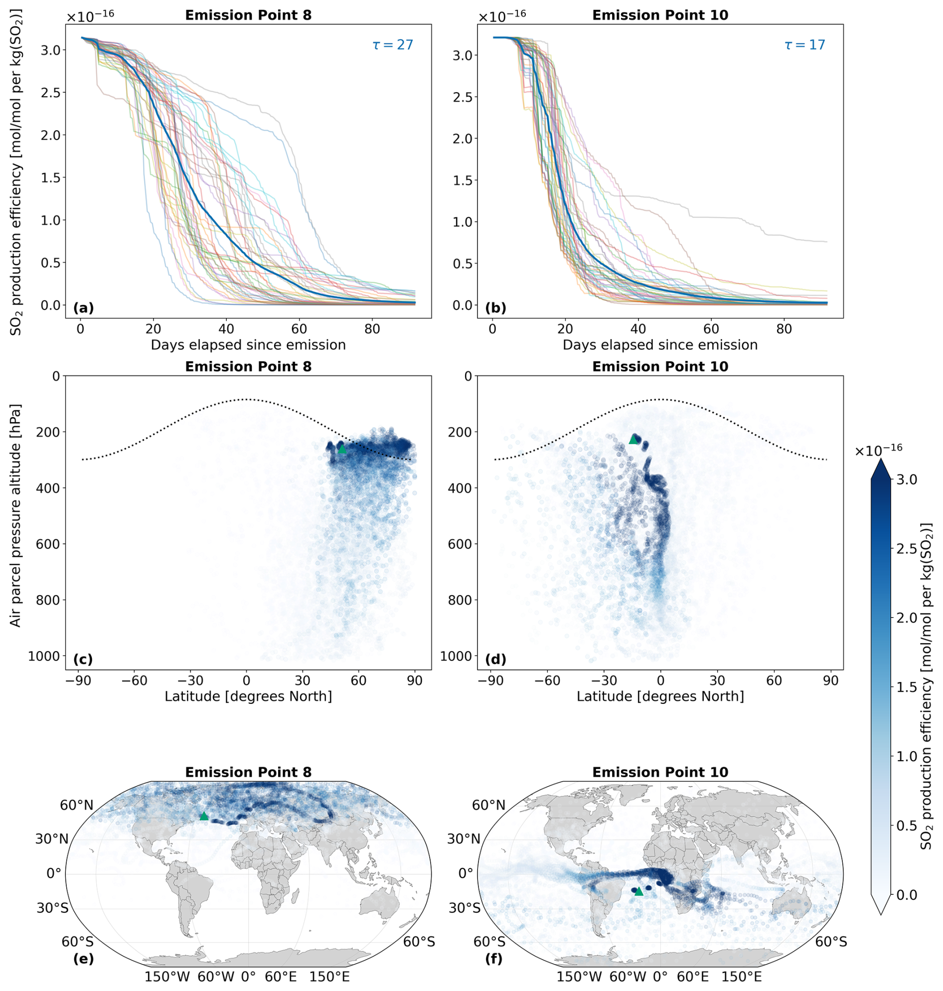
Figure 5 The spatio-temporal variation of aviation-emitted sulfur dioxide (SO₂) scaled by the emission mass for emission points 8 and 10 (see Fig. 2). Panels (a)–(b) display the temporal evolution of the SO₂ production efficiency throughout the 90 d simulation period (July–September 2015). The multi-colored lines denote the production efficiencies across 50 air parcel trajectories initialized at the selected emission points. The thicker dark blue curve is the mean of these 50 trajectories. The values of τ represent the e-folding times in days for this mean curve. Panels (c)–(d) present the spatial variation of the production efficiency as a function of the pressure altitude and latitude. The dotted black line denotes the climatological tropopause. Panels (e)–(f) illustrate the spatial variation of the production efficiency as a function of latitude and longitude. The green triangles indicate the approximate location of emission points 8 and 10.

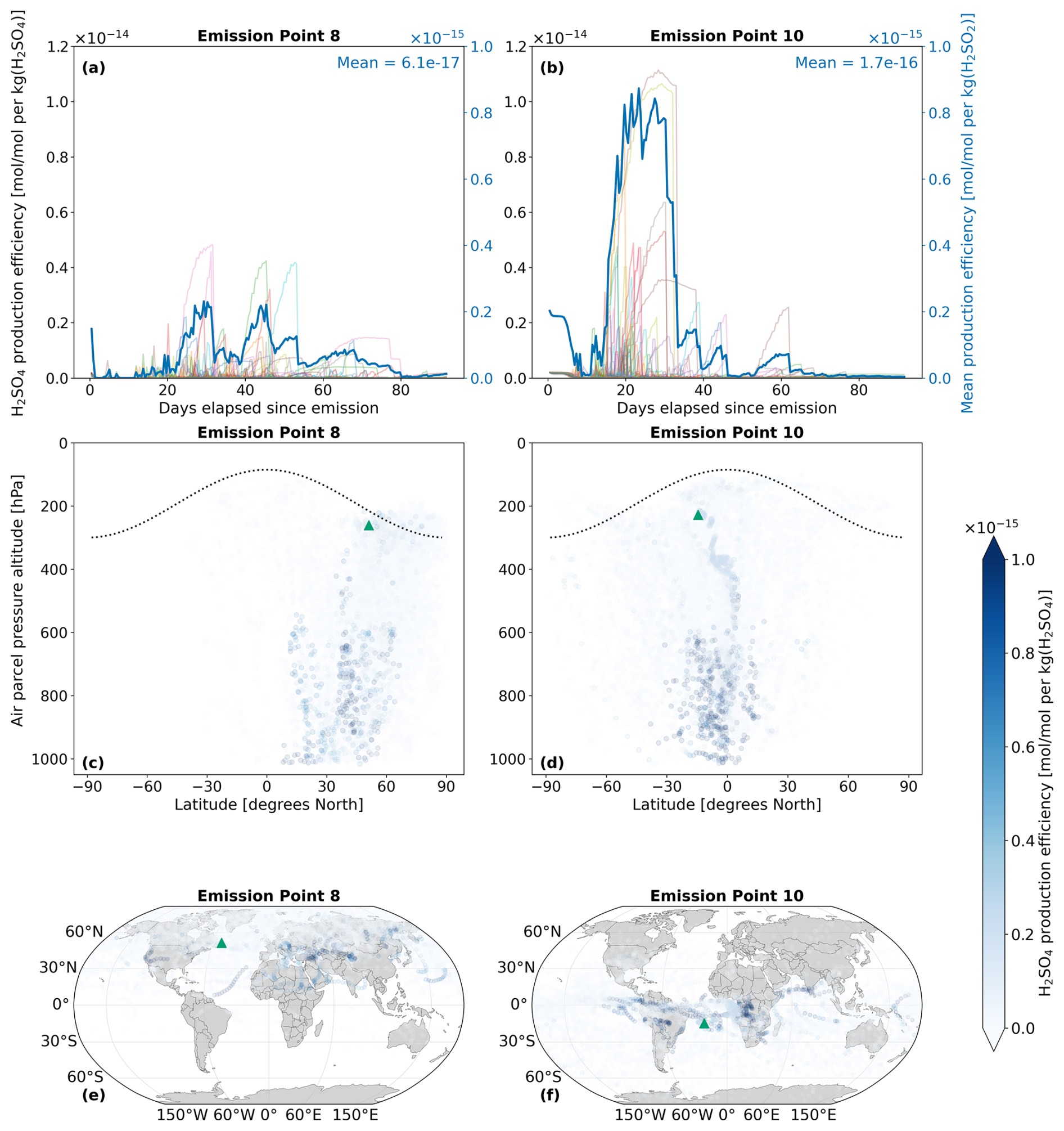
Figure 6 The spatio-temporal variation of aviation-emitted sulfuric acid (H₂SO₄) scaled by the emission mass for emission points 8 and 10 (see Fig. 2). Panels (a)–(b) display the temporal evolution of the H₂SO₄ production efficiency throughout the 90 d simulation period (July–September 2015). The multi-colored lines denote the production efficiencies across 50 air parcel trajectories initialized at the selected emission points. The thicker dark blue curve is the mean of these 50 trajectories. Panels (c)–(d) present the spatial variation of the production efficiency as a function of the pressure altitude and latitude. The dotted black line denotes the climatological tropopause. Panels (e)–(f) present the spatial variation of the production efficiency as a function of latitude and longitude. The green triangles show the approximate location of emission points 8 and 10.

4.2 Analysis of secondary SO₄

The amount of sulfate attributable to aviation emissions of SO₂ and H₂SO₄ is calculated according to Eqs. (24) and (25). Figure 7 displays the spatio-temporal evolution of total sulfate, which is defined as the sum of SO₄ across the nine aerosol modes mentioned in Sect. 2.3: ${\mathrm{SO}}_{\mathrm{4}}=\sum _{i=\mathrm{1}}^{\mathrm{9}}{\mathrm{SO}}_{\mathrm{4},i}$. On average, SO₄ production at emission point 10 (Fig. 7b) is nearly three times larger than at emission point 8 (Fig. 7a). This large discrepancy is owed to the significantly larger amount of H₂SO₄ that results from point 10, which is converted to SO₄ via processes like nucleation and condensation. Both Fig. 7a and b further exemplify this, as SO₄ production is initiated when H₂SO₄ production is maximal, which occurs approximately at the 30 d mark for point 8 (Fig. 6a) and at the 20 d mark for point 10 (Fig. 6b). As there is an approximate 20 d delay from the emission of SO₂ and H₂SO₄ until the point during which SO₄ production occurs, sulfate aerosols can form in regions far from the initial emission points, as was seen with H₂SO₄ in Fig. 6. The sulfate lifetimes approximate to 67 and 64 d for points 8 and 10, respectively. Unlike precursor species such as SO₂, secondary sulfate exhibits significantly longer atmospheric lifetimes – ranging from several days to weeks in the troposphere (Textor et al., 2006; Boucher, 2015; Toohey et al., 2025), and extending to several months or even years in the stratosphere (Myhre et al., 2013; Sun et al., 2024; Toohey et al., 2025). The lifetimes estimated in this study are comparable to the upper end of the tropospheric range, likely due to the consideration of pulse emissions in the UTLS and fall well within the expected stratospheric range. A more detailed discussion of these calculations is provided in Sect. 4.3.

Regarding the spatial distribution of SO₄, flying at point 8 on that specific day is likely to lead to the strongest sulfate production in the Northern Hemisphere, between the latitudes of 30 and 60° N (Fig. 7c). The vertical SO₄ profiles for all emission points and both simulation periods may be consulted in Figs. S16 and S19 in the Supplement. According to the corresponding horizontal distribution panel (Fig. 7e), several regions beyond the local North Atlantic emission area are affected, including parts of Europe and Asia. For point 10, a wider latitudinal band is impacted, with the largest impacts noted between 0 and 60° S (Fig. 7d). The Pacific region close to the Equator is likely to experience the largest SO₄ production (Fig. 7f). The Brewer-Dobson Circulation (BDC) patterns might also impact the vertical transport of sulfate. As has been noted by Sun et al. (2023), particles injected in the Tropics at around the upper troposphere and lower stratosphere closer to the Equator will generally experience upwelling and may be transported higher into the stratosphere via the deep branch of the BDC. This phenomenon is likely observed in Fig. 7c and d, where air parcels rise above the emission point (green triangle) and reach the highest altitudes near 0° N. The highest point reached for an emission starting at point 8 is 103 hPa (∼ 16.1 km) and for point 10 is 94 hPa (∼ 16.7 km). Additionally, as emission point 10 is closer to the Equator, more sulfate aerosols are lofted into the stratosphere, which enhances sulfate VMRs at higher altitudes and may even prolong the overall lifetime of aerosols if they remain in the stratosphere.

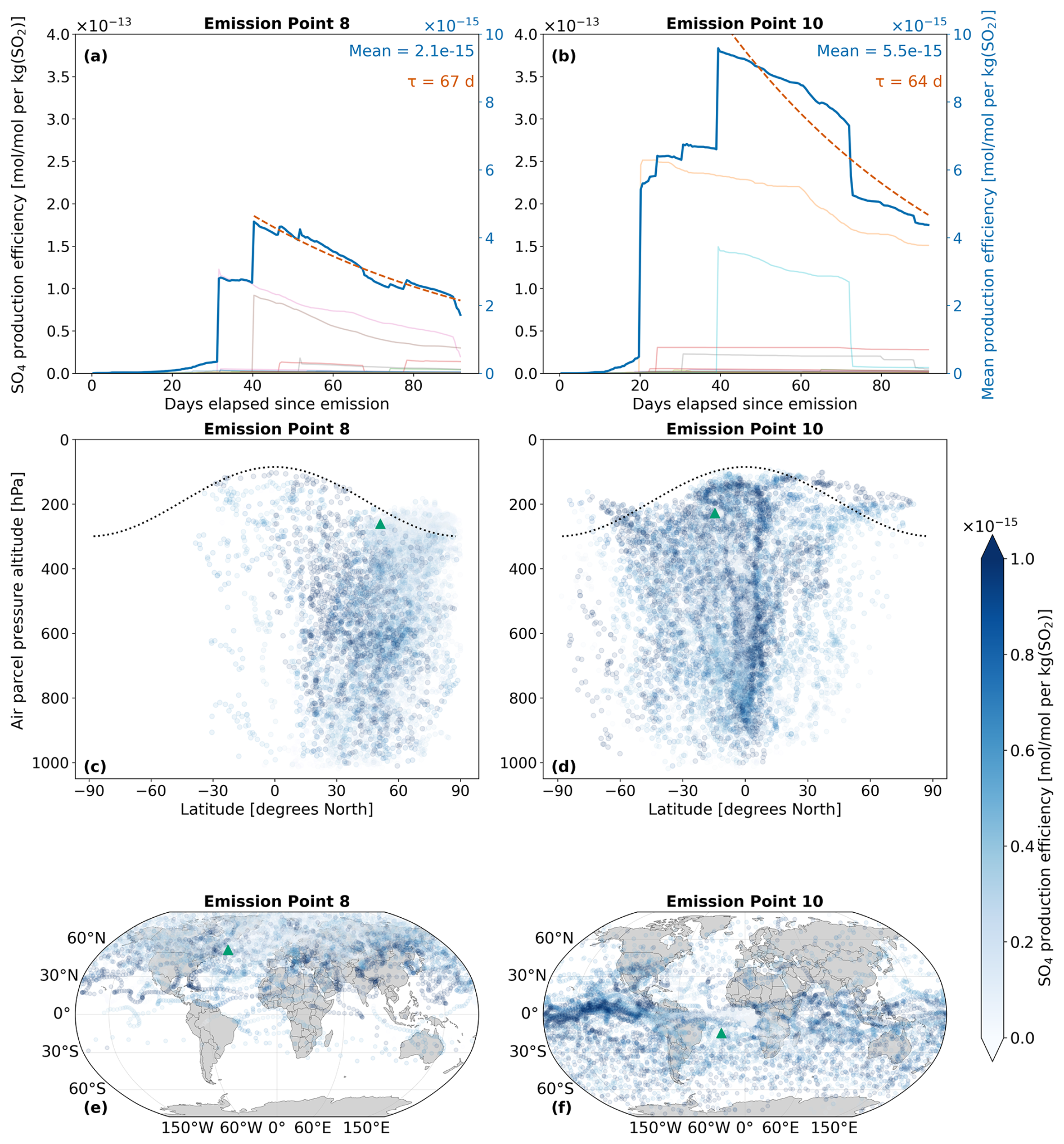
Figure 7 The spatio-temporal variation of aviation-emitted total sulfate (sum of nine modes of SO₄) scaled by the emission mass for emission points 8 and 10 (see Fig. 2). Panels (a)–(b) display the temporal evolution of the SO₄ production efficiency throughout the 90 d simulation (July–September 2015). The multi-colored lines denote the production efficiencies across 50 air parcel trajectories initialized at the selected emission points. The thicker dark blue curve is the mean of these 50 trajectories. The e-folding time (τ) in days is shown in red and corresponding exponential lifetime fits are shown by the dashed red curves. Panels (c)–(d) present the spatial variation of the production efficiency as a function of the pressure altitude and latitude. The black dotted line denotes the climatological tropopause. Panels (e)–(f) illustrate the spatial variation of the production efficiency as a function of latitude and longitude. The green triangles indicate the approximate location of emission points 8 and 10.

4.3 Intra-annual variability

The production of sulfate aerosols from aviation exhibits a strong seasonal dependence driven by the variability in background chemistry and solar radiation. Seasonal changes in the background water vapor and HO_x levels may influence the oxidation pathways that convert SO₂ into SO₄. It is also worth noting that years 2015 and 2016 were characterized by an extreme El Niño event (Paek et al., 2017). Our analysis is based on a single simulation year, so the differences across both simulation periods shown in Fig. 8 may reflect both seasonal variability and interannual anomalies, rather than the climatological seasonal cycle alone. We therefore interpret the January to March and July to September periods as contrasting background states in different seasons to assess model sensitivity, not to quantify the climatological seasonal cycle.

Among the relevant background variables, OH is particularly important. The SO₂ lifetime depends on the OH radical, which drives its gas-phase oxidation. OH is prevalent in warm and humid locations as its formation relies on the photodissociation of O₃ and subsequent reaction with H₂O (Riedel and Lassey, 2008). Figure 8a depicts the range of SO₂ e-folding times for both periods. The median e-folding time of 22 d in January (winter) is nearly 60 % larger than the median of 14 d in July (summer), which is expected, given the increased solar radiation during summer that contributes to increased OH and faster SO₂ depletion rates. Consequently, this enhanced oxidation of SO₂ results in larger SO₄ production, as shown in Fig. 8b, where its median production efficiency is 144 % larger in July compared to January. The summertime SO₂ median lifetime of 14 d is within the upper limit from past studies (Von Glasow et al., 2009), while our wintertime estimate of 22 d is slightly overestimated. This may be explained by our simplification of not accounting for the rapid aqueous-phase oxidation in the troposphere and scavenging processes, which act as significant SO₂ sinks. However, our wintertime range of SO₂ e-folding estimates agrees with results of the modeling study by Zhu et al. (2022) and with the observations from the 2022 Hunga Eruption from the Infrared Atmospheric Sounding Interferometer (IASI) satellite instrument that also estimated a similar upper limit lifetime of 21.4 d (Sellitto et al., 2024). Due to the skewed nature of the distributions shown in Fig. 8, a non-parametric statistical approach is more appropriate than parametric alternatives that assume normality. Therefore, the Mann-Whitney U test (Mann and Whitney, 1947) was applied to assess the statistical significance of differences across the two seasons. Based on this test, both the SO₂ lifetime (p-value $=\mathrm{3.57}\times {\mathrm{10}}^{-\mathrm{4}}$) and the SO₄ mean production efficiencies (p-value $=\mathrm{6.83}\times {\mathrm{10}}^{-\mathrm{3}}$) are found to be statistically significantly larger at the 95 % confidence level during the winter and summer seasons, respectively.

The lifetime of sulfate (Fig. 8c) has a median close to 2 months, with a value of around 62 d in January and 65 d in July. Unlike SO₂, the median SO₄ lifetimes are not statistically significantly different across summer and winter according to the same test statistic and confidence interval mentioned earlier (p-value = 0.55). It is worth noting, however, that the maximum SO₄ lifetime during winter of 123.5 d is almost 30 % larger than the maximum in summer (96.7 d). This causes the mean SO₄ lifetime to be larger in January (69 d) than in July (67 d). The sulfate time series plots for all 28 emissions points for the periods January–March and July–September 2015 from which the e-folding times in Fig. 8 were calculated are shown in Figs. S5 and S6 in the Supplement (Maruhashi et al., 2025b).

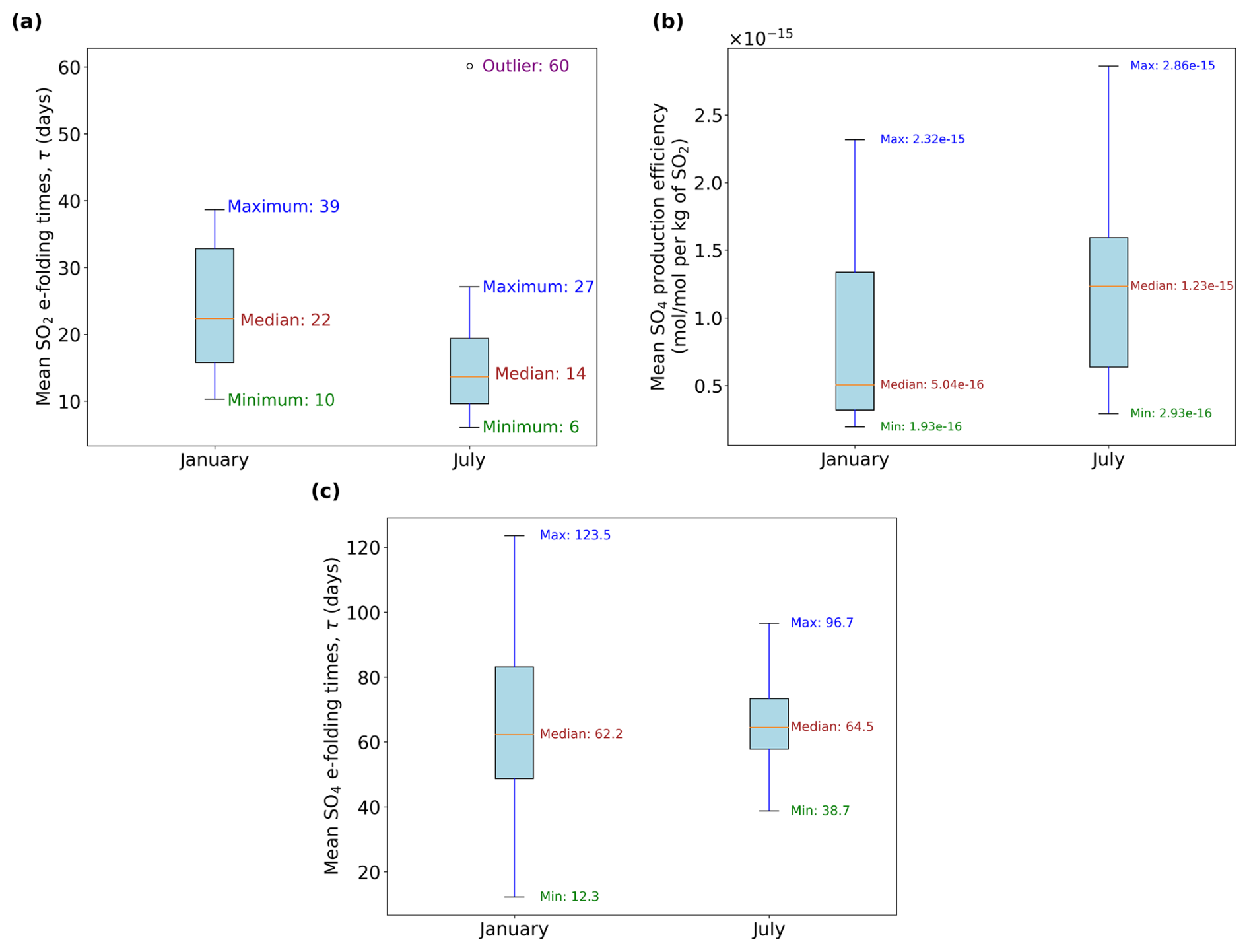
Figure 8 Intra-annual comparison across different seasons of (a) sulfur dioxide (SO₂) e-folding times (e.g. same τ values in Fig. 5), (b) the three-month mean sulfate (SO₄) production efficiencies and (c) the sulfate e-folding times. Outliers in (b) are not shown for clarity. The horizontal axes describe the month of emission where “January” denotes the period January–March 2015 and “July” denotes July–September 2015.

Our range of calculated SO₄ lifetimes is consistent with output from another Lagrangian passive tracer pulse experiment from Toohey et al. (2025) that employs the FLEXPART model. In their analysis, stratospheric sulfate aerosol transport and lifetimes were analyzed in the context of volcanic SO₂ eruptions in the Northern Hemisphere. The altitudinal range of tracer injections in December and June that they considered varies from 13–25 km, where SO₄ aerosol lifetimes increased sharply with altitude. Since we emit SO₂ pulses at the UTLS that lead to sulfate maxima reaching around 100 hPa (∼ 16 km) according to Fig. 7c and d, our results will also be comparable to theirs. According to their Fig. 4, sulfate aerosols at an altitude of 13 km between 40 and 60° N exhibit lifetimes ranging from 1.9 to 3.9 months during June (summer) and from 3.4 to 4 months during December (winter). Our Fig. 8c displays a median value of 62 d or ∼ 2.1 months for January and ∼ 2.2 months for July. Our estimates are expectedly lower than their estimated range given our lower emission altitude. Furthermore, seeing as there is a portion of sulfate that reaches the stratosphere at around 16 km in altitude (e.g. Fig. 7), upper bound values in Fig. 8c such as 96.7 d (∼ 3.2 months) in July and 123.5 d (∼ 4.1 months) in January are also justified bearing in mind that, Sun et al. (2023), for instance, for an injection height of 16 km, found particle lifetimes throughout the year that ranged from 2.4 to 9.6 months, which are similar to both of our seasonal estimates from Fig. 8c. Sun et al. (2024) inferred a shorter lower-stratospheric aerosol lifetime of 4.8 months at 65 hPa (∼ 18.5 km). By contrast, particle lifetimes according to Toohey et al. (2025) for an injection height of 15 km were longer, ranging from 6.1–7.5 months. Differences between estimates from AIRTRAC and other models like LAGRANTO are, however, naturally expected as the latter does not consider aerosol microphysical processes like particle growth along trajectories.

4.4 Application to aerosol-cloud interactions

To demonstrate the capability of AIRTRAC v2.0 in predicting when aviation-attributable sulfate aerosols will likely interact with low-level liquid clouds, we incorporate satellite data from ESA's Climate Change Initiative (CCI) to identify the approximate locations of these clouds. More specifically, version 3 of the Advanced Very High Resolution Radiometer ante meridiem dataset (AVHRR-AMv3; Stengel et al., 2019) at monthly means is used, which covers the period from 1982 to 2016. This comprehensive dataset comprises 174 variables with a latitude-longitude grid resolution of 0.5° × 0.5°. To pinpoint the location of liquid clouds during the simulated periods in summer and winter, the liquid cloud fraction (LCF) and cloud top pressure (CTP) variables were analyzed.

Based on Fig. D1 from Appendix D, liquid clouds are predominantly found at CTPs below 800 hPa and are primarily concentrated in the Northern Atlantic, Northern Pacific and Southern Tropics, with a notably larger mean LCF observed during the summer months (July–September 2015). During this period, liquid clouds frequently form in the Southern Tropical Belt, between 0–30° S across all longitudes. These horizontal liquid cloud distributions are consistent with those reported by Stengel et al. (2020) for June 2014 and with those from Muhlbauer et al. (2014), who used CloudSat/CALIPSO data from 2006 to 2011. Similarly, Lauer et al. (2007), using annual mean satellite data from the International Satellite Cloud Climatology Project (ISCCP) for the period 1983–2004, confirm a significant presence of low-level liquid clouds in the North Atlantic, North Pacific and South Atlantic regions.

Based on observations from the AVHRR-AMv3 cloud satellite dataset, one of the main regions with predominant low-level liquid cloud formation between July–September 2015 is marked with a blue rectangle in Fig. 9. When emissions occur near the Northern Mid-latitudes during summer (Fig. 9a), SO₄ may have an extended residence time near the cruise altitude, resulting in a slower downward transport to lower altitudes. The dark blue median trajectory shows that air parcels following this path remain close to the emission pressure altitude of approximately 240 hPa for around 8 d before descending towards the surface, eventually reaching latitudes between 30–60° N. Although it is unlikely that SO₄ from emission point 8 will reach the Southern Tropical Belt with liquid clouds indicated by the blue rectangle, it could still interact with some liquid clouds present in the North Atlantic and in the North Pacific (see Fig. D1a and b). In contrast, emissions at point 10 in the Southern Tropics (Fig. 9b) present an increased likelihood for interactions between aviation sulfate and liquid clouds in the Southern Tropical Belt.

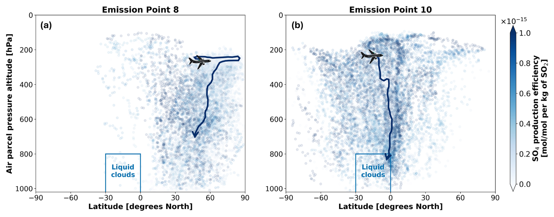
Figure 9 Transport patterns for aviation-induced sulfate aerosols when SO₂ and H₂SO₄ are jointly emitted during July–September 2015 at (a) emission point 8 and at (b) emission point 10. The dark blue arrows emanating from the aircraft represent the approximate median trajectories in each case. The aircraft icon indicates the approximate emission point. The blue rectangle denotes the probable location of lower-level liquid cloud formation in the Southern Tropical Belt between July–September of 2015 according to the AVHRR-AMv3 dataset.

5 Evaluation of AIRTRAC v2.0

The conservation of sulfur species (closed mass budget) across the microphysical aerosol tendencies from MADE3 (growth, aging, coagulation, condensation and nucleation) that AIRTRAC v2.0 scales has been validated by Sharma et al. (2025). In general, the direct evaluation of tagging models using observational data is difficult, since observed concentrations of chemical species are total quantities that emanate from various sources, both biogenic and anthropogenic, and disentangling these categories is challenging. Direct observational data for benchmarking are therefore unavailable. From a modeling perspective, evaluation is also challenging as many Lagrangian models are geared towards the stratospheric analysis of sulfate, as has been referred in earlier sections. However, the underlying components and submodels linked to AIRTRAC, like MADE3, have been extensively evaluated against a variety of experimental data (Kaiser et al., 2019). The lifetimes calculated by AIRTRAC v2.0 of precursor species like SO₂ and secondary SO₄ have also been shown to agree reasonably well in Sect. 4.1 and 4.3 respectively with the output from other Lagrangian models applied to the study of stratospheric SO₄ from volcanic pulse emissions of SO₂ (Sun et al., 2023; Sun et al., 2024; Toohey et al., 2025). To evaluate the spatial distribution patterns of SO₄, a perturbation approach using a modeling setup similar to Righi et al. (2023) was applied. This simulation setup provides the most suitable basis for comparison due to its use of the same EMAC submodels and emissions inventories (i.e. the same aviation SO₂ mass fluxes from CMIP6 for the year 2015), ensuring consistent background conditions. Additionally, for increased comparability, the CMIP6 aviation SO₂ emissions inventory applied in the perturbation method has been modified to only consider mass fluxes at the same pressure level of 240 hPa. It is important to reiterate that while the spatial patterns of SO₄ can be meaningfully compared, the magnitudes from the tagging and perturbation approaches are not expected to match, as each method addresses fundamentally different research questions (Clappier et al., 2017).

Figure 10 presents a comparison of the VMRs for SO₄ according to AIRTRAC v2.0 (Fig. 10a and c) and the perturbation approach (Fig. 10b and d) for both simulation periods. In AIRTRAC simulations, each of the 28 points (Fig. 2) is treated as an independent emission scenario, with no chemical interaction between any of the emissions considered (Maruhashi et al., 2024). Consequently, the values in Fig. 10a and c represent the total sulfate VMR across all 28 points and nine aerosol modes. However, a direct comparison of magnitudes is still challenging, as the perturbation approach inherently accounts for background feedbacks (i.e. local saturation effects and depletion of oxidizing species like OH) and non-linear interactions across emissions. Furthermore, the nature of emissions is also different: 15 min pulses are applied for AIRTRAC, and sustained emissions across three months are assumed for the perturbation method. Although a direct comparison of magnitudes is difficult, both methods yield estimates of the same order of magnitude, i.e., 10⁻¹² mol mol⁻¹.

Both methods reveal similar transport patterns, highlighting a production lag of sulfate relative to SO₂ emissions. This is evident in the larger VMRs that appear at altitudes below the original emission level of 240 hPa. Both approaches also agree that the tropical latitudinal band between 0 and 20° N near the surface is most strongly affected, in line with the results of Righi et al. (2023) for total aviation SO₄ in 2015 (see their Fig. S15b). While both methods capture enhanced VMRs near the emission altitude (∼ 200 hPa), the perturbation approach predicts stronger sulfate concentrations in the upper northern latitudes (above 40° N; Fig. 10b, d) during both seasons, which is again consistent with Righi et al. (2023). AIRTRAC, by contrast, produces larger VMRs at this altitude closer to the northern tropics and mid-latitudes (Fig. 10a, c). This discrepancy may arise because the perturbation approach assumes a more widespread distribution of SO₂ given the sustained nature of its emissions, whereas AIRTRAC transports 15 min pulse emissions that are largest in magnitude over the mid-latitudes between 30 and 40° N (e.g. emission points 4, 7, 15 and 18 in Fig. 2).

During winter, both approaches predict an enhancement of sulfate near the surface in the tropics (Fig. 10a and b). Close to a pressure altitude of 400 hPa, the perturbation approach estimates considerably smaller VMRs at the tropics. This could arise from feedbacks that mask effects (similar to chemical applications, see Grewe et al., 2012) or from the consideration that only 10 out of 28 emission points are located below 30° N, where individually they represent smaller emissions compared to, for instance, points 7 and 15 in Fig. 2. During summer, discrepancies between the approaches are larger, both near the surface and close to altitudes between 400 and 500 hPa (Fig. 10c and d). However, the region with the largest VMRs occurs below 600 hPa for both models and in the latitudinal band between 0–40° N. At the lowermost layers, AIRTRAC estimates negligible SO₄ VMRs, which could be due to the inherent limitations from the Lagrangian advection scheme itself, performed by the ATTILA submodel (Reithmeier and Sausen, 2002; Brinkop and Jöckel, 2019). As the grid-point equivalent VMRs are calculated based on the average VMRs across all air parcels in a grid box, and the distribution of air parcels is not strictly always representative of the pressure and air density distribution in the grid space, the mapping between Lagrangian space and Eulerian frames may lead to differences in the calculation of VMRs of the air parcels (Grewe et al., 2014b). Additionally, AIRTRAC estimates are also conditioned by the number of air parcels per grid box. According to Reithmeier and Sausen (2002), the average number of air parcels near the surface for a T30 resolution is between 0.25 and 0.5 (see their Fig. 1). This could also explain the much smaller VMRs near the surface in Fig. 10a and c.

Another source for the discrepancies between the spatial patterns in Fig. 10 could be the linear parameterization for the mixing between air parcels by the LGTMIX submodel. The mixing intensity is controlled by two constants ($d_{\mathrm{trop}}={\mathrm{10}}^{-\mathrm{3}}$;$d_{\mathrm{strat}}={\mathrm{10}}^{-\mathrm{6}}$), one for each layer of the atmosphere. These were initially proposed by Collins et al. (1997) for gases and d_strat was later changed to $\mathrm{5}\times {\mathrm{10}}^{-\mathrm{4}}$ by Reithmeier and Sausen (2002). Although short-lived species have been shown to be less sensitive to these parameters (Reithmeier and Sausen, 2002), the suitability of these constants to model aerosol mixing within air parcels has not been assessed. Further on the topic of linearization, AIRTRAC's linearly independent SO₄ contribution estimates for each emission point are added to yield the total SO₄ (includes all nine modes) field in Fig. 10. In contrast to the perturbation approach, this total neglects non-linear interaction effects between pulse emissions. For aviation NO_x–O₃ interactions, such non-linearities have the capability to alter production efficiencies by up to 30 % (Maruhashi et al., 2024). Ultimately, however, the sulfate spatial distributions between AIRTRAC and the perturbation approach largely agree that the lower altitudes between the tropical to mid-latitudinal bands are the most affected. Despite methodological (tagging vs. perturbation) and emission type (pulse vs. sustained) discrepancies, both approaches still yield estimates within the same order of magnitude.

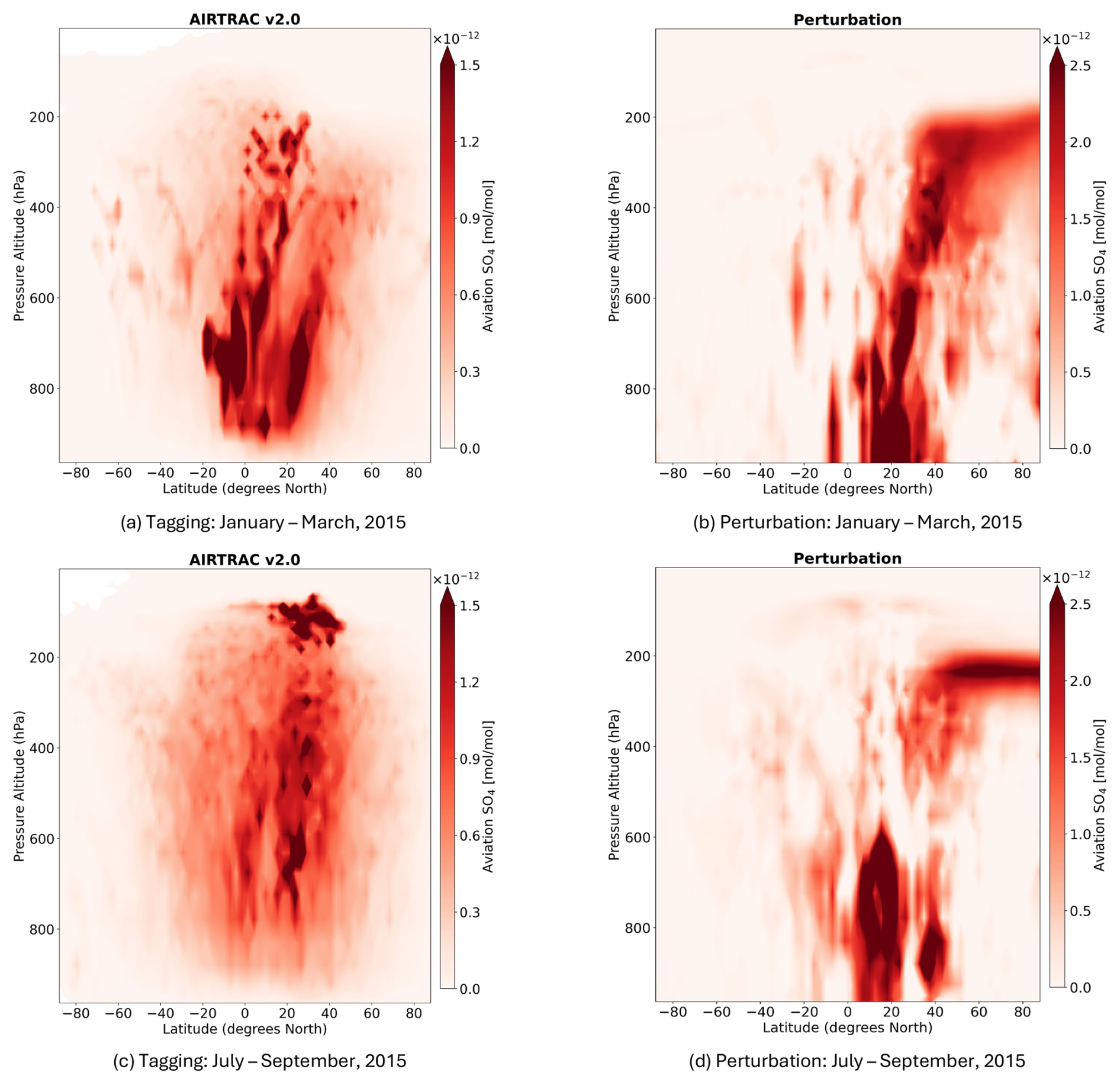
Figure 10 Comparison of AIRTRAC's tagging estimates with the MADE3-based perturbation approach using a modeling setup similar to Righi et al. (2023) for total SO₄ (sum of nine aerosol modes) during the period January–March for (a) and (b) and July–September 2015 for (c) and (d). Estimates from AIRTRAC v2.0 (a, c) represent the sum across all 28 emission points of the total SO₄ at each of these points.

6 Discussion and conclusion

6.1 Model advances, limitations and future research

AIRTRAC v2.0 is the first Lagrangian sulfate tagging scheme within EMAC, providing the unique capability to track the long-range atmospheric evolution of aviation-emitted sulfur compounds. Starting from the emission of SO₂ and H₂SO₄ at subsonic cruise altitudes, the scheme follows their chemical transformation into SO₄ followed by the subsequent descent of these aerosols into the lower troposphere. By considering aerosol microphysical processes like nucleation, condensation, coagulation, aging and particle growth, AIRTRAC v2.0 can calculate the VMRs across nine sulfate aerosol modes. It is therefore a useful computational tool that may help predict which flight regions are most likely to lead to aerosol-cloud interactions. The quantification of these interactions and how they impact the Earth's radiative budget (i.e. in terms of radiative forcing) is a key next step.

In terms of limitations, the linearization of the production and loss tendencies from MADE3 in AIRTRAC discards climate feedback effects that could be introduced by the SO₂ and H₂SO₄ emissions. This means that locally, for instance, the atmosphere's oxidative capacity will not vary with the magnitude of the pulse emissions, meaning that background OH levels will remain unaffected by the amount of SO₂ introduced by AIRTRAC. The implications of this linearization have been analyzed in greater detail in the context of aviation NO_x-O₃ interactions by Maruhashi et al. (2024). As has been introduced in Sect. 5, the suitability of air parcel mixing parameters that were originally formulated mostly for gas-phase species still needs to be better understood. As smaller aerosols in the Aitken mode are likely to behave more closely to gaseous species when mixing and larger particles in the coarse mode will not mix as rapidly given their much larger momenta, the introduction of size-dependent mixing parameters should be considered.

Another limitation of AIRTRAC v2.0 is that it cannot track sulfate particles that have been scavenged and later re-evaporated back into the atmosphere, which may lead to underestimations of aerosol mixing ratios. Another factor potentially contributing again to the underestimation of sulfate is the exclusion of its aqueous-phase production pathway via SO₂ oxidation by O₃ and H₂O₂, due to the computational limitation discussed by Tost et al. (2006). This not only has implications for sulfate produced, but will also tend to overestimate SO₂ estimated lifetimes (Brodowsky et al., 2021). Longer SO₂ lifetimes may then also lead to longer sulfate lifetimes. Excluding plume-scale processes can lead to an overestimation of around 15 % of the aviation-induced sulfate particle number concentration, but has a negligible impact on sulfate mass when compared to an instant dispersion approach, which is adopted in AIRTRAC v2.0 (Sharma et al., 2025).

A few final considerations to further extend the capabilities of AIRTRAC v2.0 would be to firstly include the indirect impact of aviation NO_x emissions on sulfate via the production of OH by connecting its gas-phase capabilities (version 1.0) to its new aerosol capabilities. AIRTRAC could then provide a more comprehensive assessment of climate effects from aviation NO_x, which will remain relevant even for drop-in sustainable aviation fuels and emerging hydrogen-powered aircraft (Tiwari et al., 2024). This could be contemplated by updating the tagging ratio of Eq. (11) based on the bimolecular reaction formulation of the tagging equation, as was described earlier in Sect. 3.2:

$$\begin{array}{}\text{(26)}& \begin{array}{rl}& {\left.C_{{\mathrm{SO}}_{\mathrm{2}}}\right|}^{\mathrm{avi}}=\underset{\mathrm{Emission}}{\underbrace{C_{{\mathrm{SO}}_{\mathrm{2}}}(t=\mathrm{0})}}\\ & -\underset{\text{Revised tagging ratio}}{\underbrace{{\displaystyle \frac{\mathrm{1}}{\mathrm{2}}}\times \left({\displaystyle \frac{C_{{\mathrm{SO}}_{\mathrm{2}}}{|}^{\mathrm{avi}}}{C_{{\mathrm{SO}}_{\mathrm{2}}}{|}^{\mathrm{avi}}+C_{{\mathrm{SO}}_{\mathrm{2}}}{|}^{\mathrm{rem}}}}+{\displaystyle \frac{C_{\mathrm{OH}}{|}^{\mathrm{avi}}}{C_{\mathrm{OH}}{|}^{\mathrm{avi}}+C_{\mathrm{OH}}{|}^{\mathrm{rem}}}}\right)}}\\ & \times \underset{\text{Molar masses}}{\underbrace{{\displaystyle \frac{M_{{\mathrm{SO}}_{\mathrm{2}}}}{M_{{\mathrm{H}}_{\mathrm{2}}{\mathrm{SO}}_{\mathrm{4}}}}}}}\times \underset{\text{Production rate}}{\underbrace{P_{{\mathrm{H}}_{\mathrm{2}}{\mathrm{SO}}_{\mathrm{4}}}}}\times \mathrm{\Delta }t+\underset{\text{Turbulence}}{\underbrace{R\left(C_{{\mathrm{SO}}_{\mathrm{2}}}\right)}}.\end{array}\end{array}$$

Secondly, to model the influence of aviation-induced sulfate on the microphysical properties of liquid clouds (e.g. by estimating the aerosol activation into cloud condensation nuclei), it would be necessary to extend the tagging from AIRTRAC v2.0 to also include the aerosol particle number concentration, as this is a key quantity driving aerosol-cloud interactions.

Lastly, AIRTRAC has been previously used as the computational foundation for the climate change functions (CCFs), which associate a change in temperature resulting from a local emission (Grewe et al., 2014a). Thus far, only CCFs for the net NO_x effect, H₂O and contrails have been formulated for a limited set of emission points in the Northern Trans-Atlantic (Frömming et al., 2021). By running AIRTRAC v2.0, we have generated a dataset to analyze the transport of aviation-induced SO₂, H₂SO₄ and nine aerosol modes containing SO₄. This dataset may later serve as the basis for the development of the first aerosol-cloud interaction CCFs, thereby furthering the possibility of applying them to climate-optimal routing (Sausen et al., 1994; Grewe et al., 2014a).

6.2 Conclusion

This paper presents the new functionalities and technical implementation of the AIRTRAC v2.0 submodel within the EMAC modeling framework. It applies a Lagrangian tagging approach to estimate the contributions of aviation-induced SO₂ and H₂SO₄ emissions to nine aerosol modes of atmospheric sulfate. To showcase AIRTRAC's capabilities in characterizing the transport patterns of aviation sulfur compounds, two three-month simulation scenarios (across winter and summer) were performed based on the CMIP6 emissions inventory. Furthermore, ESA satellite data were incorporated to demonstrate how AIRTRAC can help predict where aviation-induced sulfate will reach lower-level liquid clouds.

The transport patterns of SO₂, H₂SO₄ and SO₄ are primarily driven by the atmospheric circulation, where trade winds and downdrafts from, e.g., subsidence events play a particularly important role. Emission latitude also influences the vertical transport pathway. In the tropics, emissions typically occur below the climatological tropopause and thus within the troposphere, where pollutants are more rapidly removed and are preferentially transported downward. At higher latitudes, emissions are more likely to be released above the tropopause, entering the stratosphere, where they are more stable and persist for longer. It was found, for instance, that SO₂ that is quickly transported to lower altitudes has a shorter atmospheric lifetime due to locally larger background concentrations of OH, which are responsible for oxidizing SO₂ and other chemical species. Furthermore, SO₂ that is transported to lower altitudes early, may lead to the largest sulfate production efficiency given the increased oxidative potential at lower tropospheric altitudes. This is consistent with past studies that have focused on NO_x (Rosanka et al., 2020). Additionally, the BDC is also influential in determining the amount of sulfate that is lofted into the stratosphere, where its lifetime is longer. For example, species emitted from points closer to the Equator may be transported higher through the upwelling of the BDC in the tropical region over time, which according to our results can reach pressure altitudes above 100 hPa. This phenomenon was also observed in another Lagrangian modeling study (Sun et al., 2023).

The SO₂ lifetime and production efficiency of SO₄ also varied across seasons in a statistically significant manner. The median lifetime of SO₂ during winter (January–March 2015) was approximately 22 d compared to 14 d during the summer (July–September 2015). The production efficiencies of SO₄ also varied intra-annually, due in part, to the dependence of OH concentrations on solar radiation: summer brings increased sunlight that enhances OH production, thereby boosting SO₄ formation. Overall, there was a 40 % reduction of SO₂ lifetimes in summer relative to winter and the SO₄ production efficiency in summer was 144 % larger, these differences were found to be statistically significant at a 95 % confidence level. Although median sulfate lifetimes were found to be larger in summer, by almost 4 %, the maximum SO₄ lifetime during winter was approximately 30 % larger than in summer. The differences in SO₄ lifetimes were not found to be statistically significant.

We also present a case study illustrating how AIRTRAC v2.0 can be used to assess whether SO₂ emitted at cruise altitude is transported downward to levels more conducive to liquid-cloud formation, as indicated by ESA satellite cloud data. A clear difference was found between two emission scenarios: emitting along the North Atlantic Flight Corridor is unlikely to lead to aerosol interactions with the predominant liquid cloud cover in the Southern Tropical Belt, whereas flying at typical subsonic cruise pressure altitudes (∼ 240 hPa) in the Tropics can lead to a greater likelihood of interactions with these clouds.

AIRTRAC v2.0 relies on the aerosol tendencies from the MADE3 submodel, which have been evaluated extensively against satellite observations, in-situ aircraft measurements and ground-based station data. We have evaluated AIRTRAC v2.0 output itself, however, with a combination of other Lagrangian modeling studies and with our results from a perturbation-based modeling approach. For example, lifetime estimates of SO₂ and SO₄ have been compared with both modeling and observational studies of sulfate formation from volcanic eruptions, which can likewise be represented as a pulse emission of SO₂ at an above-surface injection altitude, followed by the production of SO₄ and its transport into the stratosphere. Given that some of our sulfate emissions also reach the stratosphere at similar injection heights tested by these studies, we have used them as reference. Our median SO₂ lifetimes agree mostly well with these past estimates ranging between a couple of days to three weeks. Our median SO₄ lifetimes of 2.1 and 2.2 months in January and July, respectively, likewise agree. To assess the spatial distribution patterns of SO₄ predicted by AIRTRAC v2.0, we performed additional perturbation simulations with a comparable setup. Results showed that both approaches are consistent in identifying a similar latitudinal band in which sulfate VMR maxima are found in the lower troposphere. The near-surface estimates differ the most, where such discrepancies are likely owed to the limitations of a Lagrangian approach in having fewer air parcels near the surface (∼ 0.25–0.5 per grid box) compared to higher parts of the atmosphere, where around 12–24 times as many air parcels can exist per grid box.

Overall, AIRTRAC v2.0 is a promising tool that estimates lifetimes of sulfur-based species that drive aerosol-cloud interactions. Additionally, it can map the spatial distribution patterns to predict the emission points that are more likely to lead to impacts on lower-level liquid clouds. It is also highly efficient, capable of calculating up to around 28 emission scenarios in a single simulation, depending on the characteristics of the high-performance cluster.

Appendix A: List of EMAC submodels applied

Table A1 List of MESSy submodels that were used for the simulations in this study. A brief description of each one is provided along with a reference that can be consulted for further information.

Appendix B: Determination of SO₂ and H₂SO₄ emission locations

We provide, in Table B1, the coordinates of the 28 emission points in Fig. 2. These have been calculated by first identifying the pressure altitude for which the zonally averaged aviation SO₂ mass flux is the largest (Fig. 3). The distribution of latitude-longitude coordinates (Fig. B1) is obtained by selecting the maximum SO₂ fluxes from the 28 grid cells with the largest SO₂ flux contributions (Eq. B1). The EP_selector tool (see Maruhashi et al. (2025a) for the full code) has been coded in Python to systematically output the coordinates of these locations by computing flux contributions across all user-defined grid cells. For those with the largest SO₂ mass flux contributions, the coordinates of the maxima are recorded. As the EP_selector tool possesses several inputs like the latitudinal and longitudinal spacing for each grid cell, as well as the number of grid cells in which to search for the n largest values, it is necessary to select an appropriate combination for these parameters. Our chosen combination is based on maximizing the total grid cells while ensuring that the total flux contribution is above 90 %.

The SO₂ mass flux contribution of grid cell i, ${\mathrm{\Gamma }}_i^{{\mathrm{SO}}_{\mathrm{2}}}$, is given by Eq. (B1):

$$\begin{array}{}\text{(B1)}& {\mathrm{\Gamma }}_i^{{\mathrm{SO}}_{\mathrm{2}}}={\displaystyle \frac{A_i\times {\mathrm{SO}}_{\mathrm{2},i}}{\sum _j^T{A}_j\times {\mathrm{SO}}_{\mathrm{2},j}}}\times \mathrm{100}\mathit{\%}.\end{array}$$

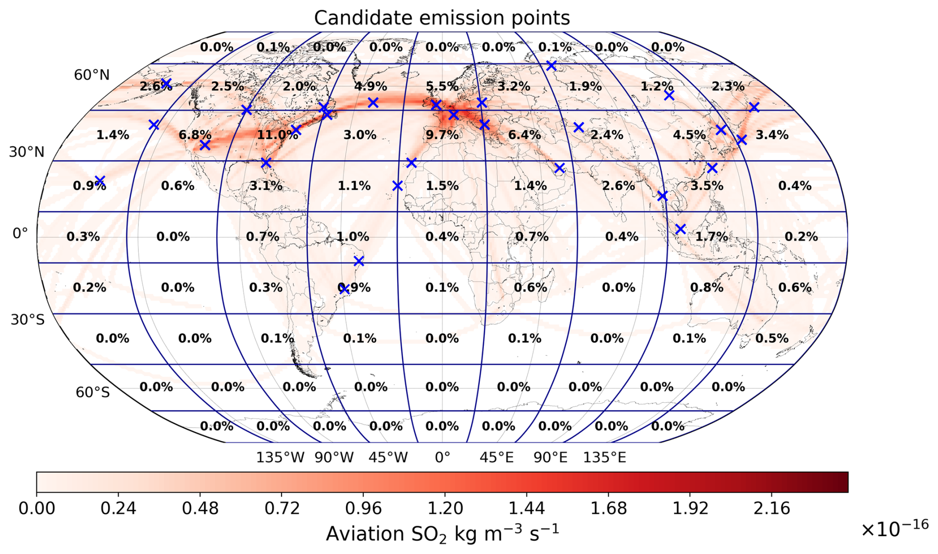
Figure B1 Horizontal distribution of the 28 emission points (blue “x” marks) determined by the EP_selector tool. The blue grid lines indicate the coarser user-defined mesh produced from spacings of 20 and 40° in the latitudinal and longitudinal directions respectively. The color bar depicts the spatial variation of aviation's SO₂ mass flux [kg m⁻³ s⁻¹] according to the CMIP6 emissions inventory. The percentages represent the contribution (Eq. B1) of a grid cell to the total SO₂ mass flux.

The total number of grid cells is given by $T=\frac{\mathrm{180}\mathit{°}}{\mathrm{\Delta }\mathrm{lat}}\times \frac{\mathrm{360}\mathit{°}}{\mathrm{\Delta }\mathrm{lon}}$, SO_2,i is the total mass within a grid cell i and the area of a grid cell A_i is calculated according to Kelly and Šavrič (2021):

$$\begin{array}{}\text{(B2)}& A_i=R_{\oplus }^{\mathrm{2}}\times \mathrm{\Delta }\mathrm{lat}\times \mathrm{\Delta }\mathrm{lon}\times \cos \stackrel{\mathrm{‾}}{{\mathrm{lat}}_i}.\end{array}$$

$\stackrel{\mathrm{‾}}{{\mathrm{lat}}_i}$ is the average between the bounding latitudes of grid cell i (i.e., the midpoint). The amount of SO₂ mass emitted in grid cell i, SO_2,i, is given by ${\mathrm{SO}}_{\mathrm{2},i}={\mathrm{\Gamma }}_i^{{\mathrm{SO}}_{\mathrm{2}}}\times {\mathrm{SO}}_{\mathrm{2},\mathrm{Total}}$, where SO_2,Total is approximately the total daily amount of SO₂ mass produced globally by aviation in 2015 according to CMIP6. The amount of H₂SO₄ is found by assuming that aviation's sulfur emissions are 98 % SO₂ and 2 % H₂SO₄. This means that the amount of H₂SO₄ mass emitted per grid cell, H₂SO_4,i, may be found in terms of SO_2,i, according to Eq. (B3):

$$\begin{array}{}\text{(B3)}& \begin{array}{rl}& {\displaystyle \frac{{\mathrm{H}}_{\mathrm{2}}{\mathrm{SO}}_{\mathrm{4},i}}{{\mathrm{H}}_{\mathrm{2}}{\mathrm{SO}}_{\mathrm{4},i}+\frac{M_{{\mathrm{H}}_{\mathrm{2}}{\mathrm{SO}}_{\mathrm{4}}}}{M_{{\mathrm{SO}}_{\mathrm{2}}}}\times {\mathrm{SO}}_{\mathrm{2},i}}}=\mathrm{0.02}\Rightarrow {\mathrm{H}}_{\mathrm{2}}{\mathrm{SO}}_{\mathrm{4},i}\\ & ={\displaystyle \frac{\mathrm{0.02}}{\mathrm{0.98}}}\times {\displaystyle \frac{M_{{\mathrm{H}}_{\mathrm{2}}{\mathrm{SO}}_{\mathrm{4}}}}{M_{{\mathrm{SO}}_{\mathrm{2}}}}}\times {\mathrm{SO}}_{\mathrm{2},i}.\end{array}\end{array}$$

The molecular masses of SO₂ and H₂SO₄ are denoted by $M_{{\mathrm{SO}}_{\mathrm{2}}}$ and $M_{{\mathrm{H}}_{\mathrm{2}}{\mathrm{SO}}_{\mathrm{4}}}$ respectively.

Table B1 SO₂ and H₂SO₄ emission point (EP) coordinates and amounts in kg. The contribution column is calculated according to Eq. (B1) and represents the area-weighted mean mass flux of a grid cell. The altitude for all locations is 238.2 hPa.

Appendix C: Tagging formulation (based on Grewe, 2013) of the coagulation process

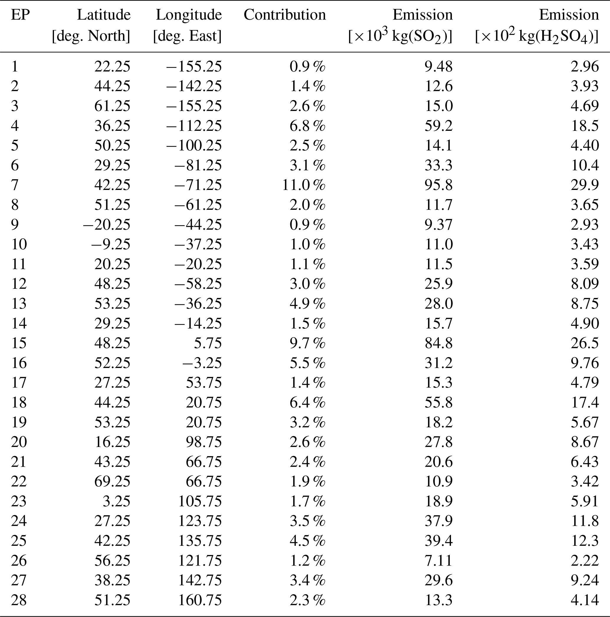
We derive the tagging formulations for the remaining eight aerosol modes by applying Eq. (9) to Eq. (6). For each mode, we first rewrite Eq. (6) into a more compact form using the notation of Eqs. (16a) and (16b) and as a function of the soluble mass fraction θ relative to water. Each derivation fulfils the tagging additivity requirement of Eq. (10). As a reminder, we note that $x_i=x_i^{\mathrm{avi}}+x_i^{\mathrm{rem}}$ and $C_p=C_{{\mathrm{NH}}_{\mathrm{4}},p}+C_{{\mathrm{NO}}_{\mathrm{3}},p}+C_{\mathrm{Na},p}+C_{\mathrm{Cl},p}+C_{\mathrm{POM},p}+C_{\mathrm{BC},p}+C_{\mathrm{DU},p}+C_{{\mathrm{H}}_{\mathrm{2}}\mathrm{O},p}$. The Brownian coagulation kernels β that influence the f_p,q terms are defined towards the end of this Appendix.

C1 Aitken mixed (km) mode

$$\begin{array}{}\text{(C1)}& \begin{array}{rl}& {\left.{\displaystyle \frac{\partial x_{\mathrm{2}}}{\partial t}}\right|}_{\mathrm{coag}}=F_{\mathrm{2}}\left(\mathit{x}\right)\\ & =\left\{\begin{array}{l}\mathrm{0};\mathit{\theta }=\mathrm{1}\left(\mathrm{Soluble}\right)\\ A\frac{x_{\mathrm{1}}}{x_{\mathrm{1}}+C_{\mathrm{1}}}-B\frac{x_{\mathrm{2}}}{x_{\mathrm{2}}+C_{\mathrm{2}}}+C\frac{x_{\mathrm{3}}}{x_{\mathrm{3}}+C_{\mathrm{3}}};\mathit{\theta }\mathit{ϵ}[\mathrm{0.1},\mathrm{1}[\left(\mathrm{Mixed}\right)\\ -{\mathrm{B}}^{\prime }\frac{x_{\mathrm{2}}}{x_{\mathrm{2}}+C_{\mathrm{2}}};\mathit{\theta }\mathit{ϵ}[\mathrm{0},\mathrm{0.1}[\left(\mathrm{Insoluble}\right)\end{array}\right.\end{array}\end{array}$$

Here, the terms A, B, B^′ and C are defined as:

$$\begin{array}{ll}{\displaystyle }& {\displaystyle }A={\mathit{\rho }}_{\mathrm{1}}{\displaystyle \frac{\mathit{\pi }}{\mathrm{6}}}\left[f_{\mathrm{1},\mathrm{2}}+f_{\mathrm{1},\mathrm{3}}\right]\\ {\displaystyle }& {\displaystyle }B={\mathit{\rho }}_{\mathrm{2}}{\displaystyle \frac{\mathit{\pi }}{\mathrm{6}}}\left[f_{\mathrm{2},\mathrm{4}}+f_{\mathrm{2},\mathrm{5}}+f_{\mathrm{2},\mathrm{6}}+f_{\mathrm{2},\mathrm{7}}+f_{\mathrm{2},\mathrm{8}}\right]\\ {\displaystyle }& {\displaystyle }{B}^{\prime }={\mathit{\rho }}_{\mathrm{2}}{\displaystyle \frac{\mathit{\pi }}{\mathrm{6}}}\left[f_{\mathrm{2},\mathrm{3}}+f_{\mathrm{2},\mathrm{6}}+f_{\mathrm{2},\mathrm{9}}\right]\\ {\displaystyle }& {\displaystyle }C={\mathit{\rho }}_{\mathrm{3}}{\displaystyle \frac{\mathit{\pi }}{\mathrm{6}}}{f}_{\mathrm{2},\mathrm{3}}^{\prime }.\end{array}$$

Aviation's contribution is then given by:

$$\begin{array}{}\text{(C2)}& \begin{array}{rl}& {\left.{\displaystyle \frac{\partial x_{\mathrm{2}}^{\mathrm{avi}}}{\partial t}}\right|}_{\mathrm{coag}}\\ & =\left\{\begin{array}{l}\mathrm{0};\mathit{\theta }=\mathrm{1}\left(\mathrm{Soluble}\right)\\ F_{\mathrm{2}}\left(\mathit{x}\right)\frac{A{C}_{\mathrm{1}}\frac{x_{\mathrm{1}}^{\mathrm{avi}}}{{\left(x_{\mathrm{1}}+C_{\mathrm{1}}\right)}^{\mathrm{2}}}-B{C}_{\mathrm{2}}\frac{x_{\mathrm{2}}^{\mathrm{avi}}}{{\left(x_{\mathrm{2}}+C_{\mathrm{2}}\right)}^{\mathrm{2}}}+C{C}_{\mathrm{3}}\frac{x_{\mathrm{3}}^{\mathrm{avi}}}{{\left(x_{\mathrm{3}}+C_{\mathrm{3}}\right)}^{\mathrm{2}}}}{A{C}_{\mathrm{1}}\frac{x_{\mathrm{1}}}{{\left(x_{\mathrm{1}}+C_{\mathrm{1}}\right)}^{\mathrm{2}}}-\mathrm{B}{C}_{\mathrm{2}}\frac{x_{\mathrm{2}}}{{\left(x_{\mathrm{2}}+C_{\mathrm{2}}\right)}^{\mathrm{2}}}+\mathrm{C}{C}_{\mathrm{3}}\frac{x_{\mathrm{3}}}{{\left(x_{\mathrm{3}}+C_{\mathrm{3}}\right)}^{\mathrm{2}}}}\\ ;\mathit{\theta }\mathit{ϵ}[\mathrm{0.1},\mathrm{1}[\left(\mathrm{Mixed}\right)\\ F_{\mathrm{2}}\left(\mathit{x}\right)\frac{x_{\mathrm{2}}^{\mathrm{avi}}}{x_{\mathrm{2}}};\mathit{\theta }\mathit{ϵ}[\mathrm{0},\mathrm{0.1}[\left(\mathrm{Insoluble}\right).\end{array}\right.\end{array}\end{array}$$

It is interesting to note that when θ=1 in Eq. (C1), the coagulation tendency is zero as there is no collision event that produces a final particle in the soluble state when one of the colliding particles is in the km mode. This is consistent with Table 2 of Kaiser et al. (2014) in which all collision events are specified.

C2 Aitken insoluble (ki) mode

$$\begin{array}{}\text{(C3)}& \begin{array}{rl}& {\left.{\displaystyle \frac{\partial x_{\mathrm{3}}}{\partial t}}\right|}_{\mathrm{coag}}=F_{\mathrm{3}}\left(\mathit{x}\right)\\ & =\left\{\begin{array}{l}\mathrm{0};\mathit{\theta }=\mathrm{1}\left(\mathrm{Soluble}\right)\\ -C\frac{x_{\mathrm{3}}}{x_{\mathrm{3}}+C_{\mathrm{3}}};\mathit{\theta }\mathit{ϵ}[\mathrm{0.1},\mathrm{1}[\left(\mathrm{Mixed}\right)\\ A^{\prime }\frac{x_{\mathrm{1}}}{x_{\mathrm{1}}+C_{\mathrm{1}}}+B^{\prime }\frac{x_{\mathrm{2}}}{x_{\mathrm{2}}+C_{\mathrm{2}}}-C^{\prime }\frac{x_{\mathrm{3}}}{x_{\mathrm{3}}+C_{\mathrm{3}}}+D^{\prime }\frac{x_{\mathrm{4}}}{x_{\mathrm{4}}+C_{\mathrm{4}}}\\ +E^{\prime }\frac{x_{\mathrm{5}}}{x_{\mathrm{5}}+C_{\mathrm{5}}};\mathit{\theta }\mathit{ϵ}[\mathrm{0},\mathrm{0.1}[\left(\mathrm{Insoluble}\right).\end{array}\right.\end{array}\end{array}$$

Here, the terms C, A^′, B^′, C^′, D^′ and E^′ are defined as:

$$\begin{array}{ll}{\displaystyle }& {\displaystyle }C={\mathit{\rho }}_{\mathrm{3}}{\displaystyle \frac{\mathit{\pi }}{\mathrm{6}}}\left[{f^{\prime }}_{\mathrm{1},\mathrm{3}}+{f^{\prime }}_{\mathrm{2},\mathrm{3}}+f_{\mathrm{3},\mathrm{4}}+f_{\mathrm{3},\mathrm{5}}+f_{\mathrm{3},\mathrm{7}}+f_{\mathrm{3},\mathrm{8}}\right]\\ {\displaystyle }& {\displaystyle }{A}^{\prime }={\mathit{\rho }}_{\mathrm{1}}{\displaystyle \frac{\mathit{\pi }}{\mathrm{6}}}{f}_{\mathrm{1},\mathrm{3}}\\ {\displaystyle }& {\displaystyle }{B}^{\prime }={\mathit{\rho }}_{\mathrm{2}}{\displaystyle \frac{\mathit{\pi }}{\mathrm{6}}}{f}_{\mathrm{2},\mathrm{3}}\\ {\displaystyle }& {\displaystyle }{C}^{\prime }={\mathit{\rho }}_{\mathrm{3}}{\displaystyle \frac{\mathit{\pi }}{\mathrm{6}}}\left[f_{\mathrm{3},\mathrm{6}}+f_{\mathrm{3},\mathrm{9}}\right]\\ {\displaystyle }& {\displaystyle }{D}^{\prime }={\mathit{\rho }}_{\mathrm{4}}{\displaystyle \frac{\mathit{\pi }}{\mathrm{6}}}{f}_{\mathrm{3},\mathrm{4}}^{\prime }\\ {\displaystyle }& {\displaystyle }{E}^{\prime }={\mathit{\rho }}_{\mathrm{5}}{\displaystyle \frac{\mathit{\pi }}{\mathrm{6}}}{f}_{\mathrm{3},\mathrm{5}}^{\prime }.\end{array}$$

Aviation's contribution is then given by:

$$\begin{array}{}\text{(C4)}& \begin{array}{rl}& {\left.{\displaystyle \frac{\partial x_{\mathrm{3}}^{\mathrm{avi}}}{\partial t}}\right|}_{\mathrm{coag}}\\ & =\left\{\begin{array}{l}\mathrm{0};\mathit{\theta }=\mathrm{1}\left(\mathrm{Soluble}\right)\\ F_{\mathrm{3}}\left(\mathit{x}\right)\frac{x_{\mathrm{3}}^{\mathrm{avi}}}{x_{\mathrm{3}}};\mathit{\theta }\mathit{ϵ}[\mathrm{0.1},\mathrm{1}[\left(\mathrm{Mixed}\right)\\ F_{\mathrm{3}}\left(\mathit{x}\right)\frac{\begin{array}{c}{A}^{\prime }{C}_{\mathrm{1}}\frac{x_{\mathrm{1}}^{\mathrm{avi}}}{{\left(x_{\mathrm{1}}+C_{\mathrm{1}}\right)}^{\mathrm{2}}}+B^{\prime }{C}_{\mathrm{2}}\frac{x_{\mathrm{2}}^{\mathrm{avi}}}{{\left(x_{\mathrm{2}}+C_{\mathrm{2}}\right)}^{\mathrm{2}}}-C^{\prime }{C}_{\mathrm{3}}\frac{x_{\mathrm{3}}^{\mathrm{avi}}}{{\left(x_{\mathrm{3}}+C_{\mathrm{3}}\right)}^{\mathrm{2}}}\\ +D^{\prime }{C}_{\mathrm{4}}\frac{x_{\mathrm{4}}^{\mathrm{avi}}}{{\left(x_{\mathrm{4}}+C_{\mathrm{4}}\right)}^{\mathrm{2}}}+E^{\prime }{C}_{\mathrm{5}}\frac{x_{\mathrm{5}}^{\mathrm{avi}}}{{\left(x_{\mathrm{5}}+C_{\mathrm{5}}\right)}^{\mathrm{2}}}\end{array}}{\begin{array}{c}A{}^{\prime }{C}_{\mathrm{1}}\frac{x_{\mathrm{1}}}{{\left(x_{\mathrm{1}}+C_{\mathrm{1}}\right)}^{\mathrm{2}}}+B^{\prime }{C}_{\mathrm{2}}\frac{x_{\mathrm{2}}}{{\left(x_{\mathrm{2}}+C_{\mathrm{2}}\right)}^{\mathrm{2}}}-C^{\prime }{C}_{\mathrm{3}}\frac{x_{\mathrm{3}}}{{\left(x_{\mathrm{3}}+C_{\mathrm{3}}\right)}^{\mathrm{2}}}\\ +D^{\prime }{C}_{\mathrm{4}}\frac{x_{\mathrm{4}}}{{\left(x_{\mathrm{4}}+C_{\mathrm{4}}\right)}^{\mathrm{2}}}+E^{\prime }{C}_{\mathrm{5}}\frac{x_{\mathrm{5}}}{{\left(x_{\mathrm{5}}+C_{\mathrm{5}}\right)}^{\mathrm{2}}}\end{array}}\\ ;\mathit{\theta }\mathit{ϵ}[\mathrm{0},\mathrm{0.1}[\left(\mathrm{Insoluble}\right).\end{array}\right.\end{array}\end{array}$$

C3 Accumulation soluble (as) mode

$$\begin{array}{}\text{(C5)}& \begin{array}{rl}& {\left.{\displaystyle \frac{\partial x_{\mathrm{4}}}{\partial t}}\right|}_{\mathrm{coag}}=F_{\mathrm{4}}\left(\mathit{x}\right)=\\ & \left\{\begin{array}{l}A\frac{x_{\mathrm{1}}}{x_{\mathrm{1}}+C_{\mathrm{1}}}-D\frac{x_{\mathrm{4}}}{x_{\mathrm{4}}+C_{\mathrm{4}}};\mathit{\theta }=\mathrm{1}\left(\mathrm{Soluble}\right)\\ -D^{\prime }\frac{x_{\mathrm{4}}}{x_{\mathrm{4}}+C_{\mathrm{4}}};\mathit{\theta }\mathit{ϵ}[\mathrm{0.1},\mathrm{1}[\left(\mathrm{Mixed}\right)\\ -D^{\prime \prime }\frac{x_{\mathrm{4}}}{x_{\mathrm{4}}+C_{\mathrm{4}}};\mathit{\theta }\mathit{ϵ}[\mathrm{0},\mathrm{0.1}[\left(\mathrm{Insoluble}\right).\end{array}\right.\end{array}\end{array}$$

Here, the terms A, D, D^′ and D^′′ are defined as:

$$\begin{array}{ll}{\displaystyle }& {\displaystyle }A={\mathit{\rho }}_{\mathrm{1}}{\displaystyle \frac{\mathit{\pi }}{\mathrm{6}}}{f}_{\mathrm{1},\mathrm{4}}\\ {\displaystyle }& {\displaystyle }D={\mathit{\rho }}_{\mathrm{4}}{\displaystyle \frac{\mathit{\pi }}{\mathrm{6}}}{f}_{\mathrm{4},\mathrm{7}}\\ {\displaystyle }& {\displaystyle }{D}^{\prime }={\mathit{\rho }}_{\mathrm{4}}{\displaystyle \frac{\mathit{\pi }}{\mathrm{6}}}\left[f_{\mathrm{2},\mathrm{4}}^{\prime }+f_{\mathrm{3},\mathrm{4}}^{\prime }+f_{\mathrm{4},\mathrm{5}}+f_{\mathrm{4},\mathrm{6}}+f_{\mathrm{4},\mathrm{8}}+f_{\mathrm{4},\mathrm{9}}\right]\\ {\displaystyle }& {\displaystyle }{D}^{\prime \prime }={\mathit{\rho }}_{\mathrm{4}}{\displaystyle \frac{\mathit{\pi }}{\mathrm{6}}}\left[f_{\mathrm{3},\mathrm{4}}^{\prime }+f_{\mathrm{4},\mathrm{6}}+f_{\mathrm{4},\mathrm{9}}\right].\end{array}$$

Aviation's contribution is given by:

$$\begin{array}{}\text{(C6)}& \begin{array}{rl}& {\left.{\displaystyle \frac{\partial x_{\mathrm{4}}^{\mathrm{avi}}}{\partial t}}\right|}_{\mathrm{coag}}=\\ & \left\{\begin{array}{l}{F}_{\mathrm{4}}\left(\mathit{x}\right)\frac{A{C}_{\mathrm{1}}\frac{x_{\mathrm{1}}^{\mathrm{avi}}}{{\left(x_{\mathrm{1}}+C_{\mathrm{1}}\right)}^{\mathrm{2}}}-D{C}_{\mathrm{4}}\frac{x_{\mathrm{4}}^{\mathrm{avi}}}{{\left(x_{\mathrm{4}}+C_{\mathrm{4}}\right)}^{\mathrm{2}}}}{A{C}_{\mathrm{1}}\frac{x_{\mathrm{1}}}{{\left(x_{\mathrm{1}}+C_{\mathrm{1}}\right)}^{\mathrm{2}}}-D{C}_{\mathrm{4}}\frac{x_{\mathrm{4}}}{{\left(x_{\mathrm{4}}+C_{\mathrm{4}}\right)}^{\mathrm{2}}}};\mathit{\theta }=\mathrm{1}\left(\mathrm{Soluble}\right)\\ F_{\mathrm{4}}\left(\mathit{x}\right)\frac{x_{\mathrm{4}}^{\mathrm{avi}}}{x_{\mathrm{4}}};\mathit{\theta }\mathit{ϵ}[\mathrm{0.1},\mathrm{1}[\left(\mathrm{Mixed}\right)\\ F_{\mathrm{4}}\left(\mathit{x}\right)\frac{x_{\mathrm{4}}^{\mathrm{avi}}}{x_{\mathrm{4}}};\mathit{\theta }\mathit{ϵ}[\mathrm{0},\mathrm{0.1}[\left(\mathrm{Insoluble}\right).\end{array}\right.\end{array}\end{array}$$

Accumulation mixed (am) mode:

$$\begin{array}{}\text{(C7)}& \begin{array}{rl}& {\left.{\displaystyle \frac{\partial x_{\mathrm{5}}}{\partial t}}\right|}_{\mathrm{coag}}=F_{\mathrm{5}}\left(\mathit{x}\right)=\\ & \left\{\begin{array}{l}\mathrm{0};\mathit{\theta }=\mathrm{1}\left(\mathrm{Soluble}\right)\\ A^{\prime }\frac{x_{\mathrm{1}}}{x_{\mathrm{1}}+C_{\mathrm{1}}}+B^{\prime }\frac{x_{\mathrm{2}}}{x_{\mathrm{2}}+C_{\mathrm{2}}}+C^{\prime }\frac{x_{\mathrm{3}}}{x_{\mathrm{3}}+C_{\mathrm{3}}}+D^{\prime }\frac{x_{\mathrm{4}}}{x_{\mathrm{4}}+C_{\mathrm{4}}}\\ -E^{\prime }\frac{x_{\mathrm{5}}}{x_{\mathrm{5}}+C_{\mathrm{5}}}+F^{\prime }\frac{x_{\mathrm{6}}}{x_{\mathrm{6}}+C_{\mathrm{6}}};\mathit{\theta }\mathit{ϵ}[\mathrm{0.1},\mathrm{1}[\left(\mathrm{Mixed}\right)\\ -E^{\prime \prime }\frac{x_{\mathrm{5}}}{x_{\mathrm{5}}+C_{\mathrm{5}}};\mathit{\theta }\mathit{ϵ}[\mathrm{0},\mathrm{0.1}[\left(\mathrm{Insoluble}\right).\end{array}\right.\end{array}\end{array}$$

Here, the terms A^′, B^′, C^′, D^′, E^′, F^′ and E^′′ are defined as:

$$\begin{array}{ll}{\displaystyle }& {\displaystyle }{A}^{\prime }={\mathit{\rho }}_{\mathrm{1}}{\displaystyle \frac{\mathit{\pi }}{\mathrm{6}}}\left[f_{\mathrm{1},\mathrm{5}}+f_{\mathrm{1},\mathrm{6}}\right]\\ {\displaystyle }& {\displaystyle }{B}^{\prime }={\mathit{\rho }}_{\mathrm{2}}{\displaystyle \frac{\mathit{\pi }}{\mathrm{6}}}\left[f_{\mathrm{2},\mathrm{4}}+f_{\mathrm{2},\mathrm{5}}+f_{\mathrm{2},\mathrm{6}}\right]\\ {\displaystyle }& {\displaystyle }{C}^{\prime }={\mathit{\rho }}_{\mathrm{3}}{\displaystyle \frac{\mathit{\pi }}{\mathrm{6}}}\left[f_{\mathrm{3},\mathrm{4}}+f_{\mathrm{3},\mathrm{5}}\right]\\ {\displaystyle }& {\displaystyle }{D}^{\prime }={\mathit{\rho }}_{\mathrm{4}}{\displaystyle \frac{\mathit{\pi }}{\mathrm{6}}}\left[f_{\mathrm{2},\mathrm{4}}^{\prime }+f_{\mathrm{3},\mathrm{4}}^{\prime }+f_{\mathrm{4},\mathrm{5}}+f_{\mathrm{4},\mathrm{6}}\right]\\ {\displaystyle }& {\displaystyle }{E}^{\prime }={\mathit{\rho }}_{\mathrm{5}}{\displaystyle \frac{\mathit{\pi }}{\mathrm{6}}}\left[f_{\mathrm{5},\mathrm{7}}+f_{\mathrm{5},\mathrm{8}}+f_{\mathrm{5},\mathrm{9}}\right]\\ {\displaystyle }& {\displaystyle }{E}^{\prime \prime }={\mathit{\rho }}_{\mathrm{5}}{\displaystyle \frac{\mathit{\pi }}{\mathrm{6}}}\left[f_{\mathrm{3},\mathrm{5}}^{\prime }+f_{\mathrm{5},\mathrm{6}}+f_{\mathrm{5},\mathrm{9}}\right]\\ {\displaystyle }& {\displaystyle }{F}^{\prime }={\mathit{\rho }}_{\mathrm{6}}{\displaystyle \frac{\mathit{\pi }}{\mathrm{6}}}\left[f_{\mathrm{1},\mathrm{6}}^{\prime }+f_{\mathrm{2},\mathrm{6}}^{\prime }+f_{\mathrm{4},\mathrm{6}}^{\prime }+f_{\mathrm{5},\mathrm{6}}^{\prime }\right].\end{array}$$

Aviation's contribution is given by:

$$\begin{array}{}\text{(C8)}& {\left.{\displaystyle \frac{\partial x_{\mathrm{5}}^{\mathrm{avi}}}{\partial t}}\right|}_{\mathrm{coag}}=\left\{\begin{array}{l}\mathrm{0};\mathit{\theta }=\mathrm{1}\left(\mathrm{Soluble}\right)\\ F_{\mathrm{5}}\left(\mathit{x}\right)\frac{n}{d};\mathit{\theta }\mathit{ϵ}[\mathrm{0.1},\mathrm{1}[\left(\mathrm{Mixed}\right)\\ F_{\mathrm{5}}\left(\mathit{x}\right)\frac{x_{\mathrm{5}}^{\mathrm{avi}}}{x_{\mathrm{5}}};\mathit{\theta }\mathit{ϵ}[\mathrm{0},\mathrm{0.1}[\left(\mathrm{Insoluble}\right).\end{array}\right.\end{array}$$

Here, n and d are abbreviations for the numerator and denominator:

$$\begin{array}{rl}n& =A^{\prime }{C}_{\mathrm{1}}{\displaystyle \frac{x_{\mathrm{1}}^{\mathrm{avi}}}{{\left(x_{\mathrm{1}}+C_{\mathrm{1}}\right)}^{\mathrm{2}}}}+B^{\prime }{C}_{\mathrm{2}}{\displaystyle \frac{x_{\mathrm{2}}^{\mathrm{avi}}}{{\left(x_{\mathrm{2}}+C_{\mathrm{2}}\right)}^{\mathrm{2}}}}+C^{\prime }{C}_{\mathrm{3}}{\displaystyle \frac{x_{\mathrm{3}}^{\mathrm{avi}}}{{\left(x_{\mathrm{3}}+C_{\mathrm{3}}\right)}^{\mathrm{2}}}}\\ & +D^{\prime }{C}_{\mathrm{4}}{\displaystyle \frac{x_{\mathrm{4}}^{\mathrm{avi}}}{{\left(x_{\mathrm{4}}+C_{\mathrm{4}}\right)}^{\mathrm{2}}}}-E^{\prime }{C}_{\mathrm{5}}{\displaystyle \frac{x_{\mathrm{5}}^{\mathrm{avi}}}{{\left(x_{\mathrm{5}}+C_{\mathrm{5}}\right)}^{\mathrm{2}}}}+F^{\prime }{C}_{\mathrm{6}}{\displaystyle \frac{x_{\mathrm{6}}^{\mathrm{avi}}}{{\left(x_{\mathrm{6}}+C_{\mathrm{6}}\right)}^{\mathrm{2}}}}\\ & d=A^{\prime }{C}_{\mathrm{1}}{\displaystyle \frac{x_{\mathrm{1}}}{{\left(x_{\mathrm{1}}+C_{\mathrm{1}}\right)}^{\mathrm{2}}}}+B^{\prime }{C}_{\mathrm{2}}{\displaystyle \frac{x_{\mathrm{2}}}{{\left(x_{\mathrm{2}}+C_{\mathrm{2}}\right)}^{\mathrm{2}}}}+C^{\prime }{C}_{\mathrm{3}}{\displaystyle \frac{x_{\mathrm{3}}}{{\left(x_{\mathrm{3}}+C_{\mathrm{3}}\right)}^{\mathrm{2}}}}\\ & +D^{\prime }{C}_{\mathrm{4}}{\displaystyle \frac{x_{\mathrm{4}}}{{\left(x_{\mathrm{4}}+C_{\mathrm{4}}\right)}^{\mathrm{2}}}}-E^{\prime }{C}_{\mathrm{5}}{\displaystyle \frac{x_{\mathrm{5}}}{{\left(x_{\mathrm{5}}+C_{\mathrm{5}}\right)}^{\mathrm{2}}}}+{\mathrm{F}}^{\prime }{C}_{\mathrm{6}}{\displaystyle \frac{x_{\mathrm{6}}}{{\left(x_{\mathrm{6}}+C_{\mathrm{6}}\right)}^{\mathrm{2}}}}\end{array}$$

C4 Accumulation insoluble (ai) mode

$$\begin{array}{}\text{(C9)}& \begin{array}{rl}& {\left.{\displaystyle \frac{\partial x_{\mathrm{6}}}{\partial t}}\right|}_{\mathrm{coag}}=F_{\mathrm{6}}\left(\mathit{x}\right)=\\ & \left\{\begin{array}{l}\begin{array}{l}\mathrm{0};\mathit{\theta }=\mathrm{1}\left(\mathrm{Soluble}\right)\\ -F\frac{x_{\mathrm{6}}}{x_{\mathrm{6}}+C_{\mathrm{6}}};\mathit{\theta }\mathit{ϵ}[\mathrm{0.1},\mathrm{1}[\left(\mathrm{Mixed}\right)\\ A^{\prime }\frac{x_{\mathrm{1}}}{x_{\mathrm{1}}+C_{\mathrm{1}}}+B^{\prime }\frac{x_{\mathrm{2}}}{x_{\mathrm{2}}+C_{\mathrm{2}}}+C^{\prime }\frac{x_{\mathrm{3}}}{x_{\mathrm{3}}+C_{\mathrm{3}}}+D^{\prime }\frac{x_{\mathrm{4}}}{x_{\mathrm{4}}+C_{\mathrm{4}}}\\ +E^{\prime }\frac{x_{\mathrm{5}}}{x_{\mathrm{5}}+C_{\mathrm{5}}}+\mathrm{\dots }\end{array}\\ -F^{\prime }\frac{x_{\mathrm{6}}}{x_{\mathrm{6}}+C_{\mathrm{6}}}+G^{\prime }\frac{x_{\mathrm{7}}}{x_{\mathrm{7}}+C_{\mathrm{7}}}+H^{\prime }\frac{x_{\mathrm{8}}}{x_{\mathrm{8}}+C_{\mathrm{8}}}\\ ;\mathit{\theta }\mathit{ϵ}[\mathrm{0},\mathrm{0.1}[\left(\mathrm{Insoluble}\right).\end{array}\right.\end{array}\end{array}$$

Here, the terms A^′, B^′, C^′, D^′, E^′, F^′, F, G^′, and H^′:

$$\begin{array}{ll}{\displaystyle }& {\displaystyle }{A}^{\prime }={\mathit{\rho }}_{\mathrm{1}}{\displaystyle \frac{\mathit{\pi }}{\mathrm{6}}}{f}_{\mathrm{1},\mathrm{6}}\\ {\displaystyle }& {\displaystyle }{B}^{\prime }={\mathit{\rho }}_{\mathrm{2}}{\displaystyle \frac{\mathit{\pi }}{\mathrm{6}}}{f}_{\mathrm{2},\mathrm{6}}\\ {\displaystyle }& {\displaystyle }{C}^{\prime }={\mathit{\rho }}_{\mathrm{3}}{\displaystyle \frac{\mathit{\pi }}{\mathrm{6}}}{f}_{\mathrm{3},\mathrm{6}}\\ {\displaystyle }& {\displaystyle }{D}^{\prime }={\mathit{\rho }}_{\mathrm{4}}{\displaystyle \frac{\mathit{\pi }}{\mathrm{6}}}{f}_{\mathrm{4},\mathrm{6}}\\ {\displaystyle }& {\displaystyle }{E}^{\prime }={\mathit{\rho }}_{\mathrm{5}}{\displaystyle \frac{\mathit{\pi }}{\mathrm{6}}}{f}_{\mathrm{5},\mathrm{6}}\\ {\displaystyle }& {\displaystyle }F={\mathit{\rho }}_{\mathrm{6}}{\displaystyle \frac{\mathit{\pi }}{\mathrm{6}}}\left[f_{\mathrm{1},\mathrm{6}}^{\prime }+f_{\mathrm{2},\mathrm{6}}+f_{\mathrm{4},\mathrm{6}}^{\prime }+f_{\mathrm{5},\mathrm{6}}^{\prime }+f_{\mathrm{6},\mathrm{7}}+f_{\mathrm{6},\mathrm{8}}\right]\\ {\displaystyle }& {\displaystyle }{F}^{\prime }={\mathit{\rho }}_{\mathrm{6}}{\displaystyle \frac{\mathit{\pi }}{\mathrm{6}}}{f}_{\mathrm{6},\mathrm{9}}\\ {\displaystyle }& {\displaystyle }{G}^{\prime }={\mathit{\rho }}_{\mathrm{7}}{\displaystyle \frac{\mathit{\pi }}{\mathrm{6}}}{f^{\prime }}_{\mathrm{6},\mathrm{7}}\\ {\displaystyle }& {\displaystyle }{H}^{\prime }={\mathit{\rho }}_{\mathrm{8}}{\displaystyle \frac{\mathit{\pi }}{\mathrm{6}}}{f^{\prime }}_{\mathrm{6},\mathrm{8}}.\end{array}$$

Aviation's contribution is given by:

$$\begin{array}{}\text{(C10)}& {\left.{\displaystyle \frac{\partial x_{\mathrm{6}}^{\mathrm{avi}}}{\partial t}}\right|}_{\mathrm{coag}}=\left\{\begin{array}{l}\mathrm{0};\mathit{\theta }=\mathrm{1}\left(\mathrm{Soluble}\right)\\ F_{\mathrm{6}}\left(\mathit{x}\right)\frac{x_{\mathrm{6}}^{\mathrm{avi}}}{x_{\mathrm{6}}};\mathit{\theta }\mathit{ϵ}[\mathrm{0.1},\mathrm{1}[\left(\mathrm{Mixed}\right)\\ F_{\mathrm{6}}\left(\mathit{x}\right)\frac{n}{d};\mathit{\theta }\mathit{ϵ}[\mathrm{0},\mathrm{0.1}[\left(\mathrm{Insoluble}\right)\end{array}\right.\end{array}$$

Here, n and d are abbreviations for the numerator and denominator:

$$\begin{array}{ll}{\displaystyle }n& {\displaystyle }=A^{\prime }{C}_{\mathrm{1}}{\displaystyle \frac{x_{\mathrm{1}}^{\mathrm{avi}}}{{\left(x_{\mathrm{1}}+C_{\mathrm{1}}\right)}^{\mathrm{2}}}}+B^{\prime }{C}_{\mathrm{2}}{\displaystyle \frac{x_{\mathrm{2}}^{\mathrm{avi}}}{{\left(x_{\mathrm{2}}+C_{\mathrm{2}}\right)}^{\mathrm{2}}}}\\ {\displaystyle }& {\displaystyle }+C^{\prime }{C}_{\mathrm{3}}{\displaystyle \frac{x_{\mathrm{3}}^{\mathrm{avi}}}{{\left(x_{\mathrm{3}}+C_{\mathrm{3}}\right)}^{\mathrm{2}}}}+D^{\prime }{C}_{\mathrm{4}}{\displaystyle \frac{x_{\mathrm{4}}^{\mathrm{avi}}}{{\left(x_{\mathrm{4}}+C_{\mathrm{4}}\right)}^{\mathrm{2}}}}\\ {\displaystyle }& {\displaystyle }+E^{\prime }{C}_{\mathrm{5}}{\displaystyle \frac{x_{\mathrm{5}}^{\mathrm{avi}}}{{\left(x_{\mathrm{5}}+C_{\mathrm{5}}\right)}^{\mathrm{2}}}}+\mathrm{\dots }\\ {\displaystyle }& {\displaystyle }-F^{\prime }{C}_{\mathrm{6}}{\displaystyle \frac{x_{\mathrm{6}}^{\mathrm{avi}}}{{\left(x_{\mathrm{6}}+C_{\mathrm{6}}\right)}^{\mathrm{2}}}}+G^{\prime }{C}_{\mathrm{7}}{\displaystyle \frac{x_{\mathrm{7}}^{\mathrm{avi}}}{{\left(x_{\mathrm{7}}+C_{\mathrm{7}}\right)}^{\mathrm{2}}}}\\ {\displaystyle }& {\displaystyle }+H^{\prime }{C}_{\mathrm{8}}{\displaystyle \frac{x_{\mathrm{8}}^{\mathrm{avi}}}{{\left(x_{\mathrm{8}}+C_{\mathrm{8}}\right)}^{\mathrm{2}}}}\\ {\displaystyle }d& {\displaystyle }=A^{\prime }{C}_{\mathrm{1}}{\displaystyle \frac{x_{\mathrm{1}}}{{\left(x_{\mathrm{1}}+C_{\mathrm{1}}\right)}^{\mathrm{2}}}}+B^{\prime }{C}_{\mathrm{2}}{\displaystyle \frac{x_{\mathrm{2}}}{{\left(x_{\mathrm{2}}+C_{\mathrm{2}}\right)}^{\mathrm{2}}}}\\ {\displaystyle }& {\displaystyle }+C^{\prime }{C}_{\mathrm{3}}{\displaystyle \frac{x_{\mathrm{3}}}{{\left(x_{\mathrm{3}}+C_{\mathrm{3}}\right)}^{\mathrm{2}}}}+D^{\prime }{C}_{\mathrm{4}}{\displaystyle \frac{x_{\mathrm{4}}}{{\left(x_{\mathrm{4}}+C_{\mathrm{4}}\right)}^{\mathrm{2}}}}\\ {\displaystyle }& {\displaystyle }+E^{\prime }{C}_{\mathrm{5}}{\displaystyle \frac{x_{\mathrm{5}}}{{\left(x_{\mathrm{5}}+C_{\mathrm{5}}\right)}^{\mathrm{2}}}}+\mathrm{\dots }\\ {\displaystyle }& {\displaystyle }-F^{\prime }{C}_{\mathrm{6}}{\displaystyle \frac{x_{\mathrm{6}}}{{\left(x_{\mathrm{6}}+C_{\mathrm{6}}\right)}^{\mathrm{2}}}}+G^{\prime }{C}_{\mathrm{7}}{\displaystyle \frac{x_{\mathrm{7}}}{{\left(x_{\mathrm{7}}+C_{\mathrm{7}}\right)}^{\mathrm{2}}}}\\ {\displaystyle }& {\displaystyle }+H^{\prime }{C}_{\mathrm{8}}{\displaystyle \frac{x_{\mathrm{8}}}{{\left(x_{\mathrm{8}}+C_{\mathrm{8}}\right)}^{\mathrm{2}}}}.\end{array}$$

C5 Coarse soluble (cs) mode

$$\begin{array}{}\text{(C11)}& \begin{array}{rl}& {\left.{\displaystyle \frac{\partial x_{\mathrm{7}}}{\partial t}}\right|}_{\mathrm{coag}}=F_{\mathrm{7}}\left(\mathit{x}\right)\\ & =\left\{\begin{array}{l}A\frac{x_{\mathrm{1}}}{x_{\mathrm{1}}+C_{\mathrm{1}}}+D\frac{x_{\mathrm{4}}}{x_{\mathrm{4}}+C_{\mathrm{4}}};\mathit{\theta }=\mathrm{1}\left(\mathrm{Soluble}\right)\\ -G^{\prime }\frac{x_{\mathrm{7}}}{x_{\mathrm{7}}+C_{\mathrm{7}}};\mathit{\theta }\mathit{ϵ}[\mathrm{0.1},\mathrm{1}[\left(\mathrm{Mixed}\right)\\ -G^{\prime \prime }\frac{x_{\mathrm{7}}}{x_{\mathrm{7}}+C_{\mathrm{7}}};\mathit{\theta }\mathit{ϵ}[\mathrm{0},\mathrm{0.1}[\left(\mathrm{Insoluble}\right).\end{array}\right.\end{array}\end{array}$$

Here, the terms A, D, G^′ and G^′′ are defined as:

$$\begin{array}{ll}{\displaystyle }& {\displaystyle }A={\mathit{\rho }}_{\mathrm{1}}{\displaystyle \frac{\mathit{\pi }}{\mathrm{6}}}{f}_{\mathrm{1},\mathrm{7}}\\ {\displaystyle }& {\displaystyle }D={\mathit{\rho }}_{\mathrm{4}}{\displaystyle \frac{\mathit{\pi }}{\mathrm{6}}}{f}_{\mathrm{4},\mathrm{7}}\\ {\displaystyle }& {\displaystyle }{G}^{\prime }={\mathit{\rho }}_{\mathrm{7}}{\displaystyle \frac{\mathit{\pi }}{\mathrm{6}}}\left[f_{\mathrm{2},\mathrm{7}}^{\prime }+f_{\mathrm{3},\mathrm{7}}^{\prime }+f_{\mathrm{5},\mathrm{7}}^{\prime }+f_{\mathrm{6},\mathrm{7}}^{\prime }+f_{\mathrm{7},\mathrm{8}}+f_{\mathrm{7},\mathrm{9}}\right]\\ {\displaystyle }& {\displaystyle }{G}^{\prime \prime }={\mathit{\rho }}_{\mathrm{7}}{\displaystyle \frac{\mathit{\pi }}{\mathrm{6}}}\left[f_{\mathrm{6},\mathrm{7}}^{\prime }+f_{\mathrm{7},\mathrm{9}}\right].\end{array}$$

Aviation's contribution is given by:

$$\begin{array}{}\text{(C12)}& \begin{array}{rl}& {\left.{\displaystyle \frac{\partial x_{\mathrm{7}}^{\mathrm{avi}}}{\partial t}}\right|}_{\mathrm{coag}}\\ & =\left\{\begin{array}{l}{F}_{\mathrm{7}}\left(\mathit{x}\right)\frac{A{C}_{\mathrm{1}}\frac{x_{\mathrm{1}}^{\mathrm{avi}}}{{\left(x_{\mathrm{1}}+C_{\mathrm{1}}\right)}^{\mathrm{2}}}+\mathrm{D}{C}_{\mathrm{4}}\frac{x_{\mathrm{4}}^{\mathrm{avi}}}{{\left(x_{\mathrm{4}}+C_{\mathrm{4}}\right)}^{\mathrm{2}}}}{A{C}_{\mathrm{1}}\frac{x_{\mathrm{1}}}{{\left(x_{\mathrm{1}}+C_{\mathrm{1}}\right)}^{\mathrm{2}}}+\mathrm{D}{C}_{\mathrm{4}}\frac{x_{\mathrm{4}}}{{\left(x_{\mathrm{4}}+C_{\mathrm{4}}\right)}^{\mathrm{2}}}}\\ ;\mathit{\theta }=\mathrm{1}\left(\mathrm{Soluble}\right)\\ F_{\mathrm{7}}\left(\mathit{x}\right)\frac{x_{\mathrm{7}}^{\mathrm{avi}}}{x_{\mathrm{7}}};\mathit{\theta }\mathit{ϵ}[\mathrm{0.1},\mathrm{1}[\left(\mathrm{Mixed}\right)\\ F_{\mathrm{7}}\left(\mathit{x}\right)\frac{x_{\mathrm{7}}^{\mathrm{avi}}}{x_{\mathrm{7}}};\mathit{\theta }\mathit{ϵ}[\mathrm{0},\mathrm{0.1}[\left(\mathrm{Insoluble}\right).\end{array}\right.\end{array}\end{array}$$

C6 Coarse mixed (cm) mode

$$\begin{array}{}\text{(C13)}& \begin{array}{rl}& {\left.{\displaystyle \frac{\partial x_{\mathrm{8}}}{\partial t}}\right|}_{\mathrm{coag}}=F_{\mathrm{8}}\left(\mathit{x}\right)\\ & =\left\{\begin{array}{l}\mathrm{0};\mathit{\theta }=\mathrm{1}\left(\mathrm{Soluble}\right)\\ A^{\prime }\frac{x_{\mathrm{1}}}{x_{\mathrm{1}}+C_{\mathrm{1}}}+B^{\prime }\frac{x_{\mathrm{2}}}{x_{\mathrm{2}}+C_{\mathrm{2}}}+C^{\prime }\frac{x_{\mathrm{3}}}{x_{\mathrm{3}}+C_{\mathrm{3}}}\\ +D^{\prime }\frac{x_{\mathrm{4}}}{x_{\mathrm{4}}+C_{\mathrm{4}}}+E^{\prime }\frac{x_{\mathrm{5}}}{x_{\mathrm{5}}+C_{\mathrm{5}}}+\mathrm{\dots }\\ \mathrm{\dots }+F^{\prime }\frac{x_{\mathrm{6}}}{x_{\mathrm{6}}+C_{\mathrm{6}}}+G^{\prime }\frac{x_{\mathrm{7}}}{x_{\mathrm{7}}+C_{\mathrm{7}}}+I^{\prime }\frac{x_{\mathrm{9}}}{x_{\mathrm{9}}+C_{\mathrm{9}}}\\ ;\mathit{\theta }\mathit{ϵ}[\mathrm{0.1},\mathrm{1}[\left(\mathrm{Mixed}\right)\\ -H^{\prime \prime }\frac{x_{\mathrm{8}}}{x_{\mathrm{8}}+C_{\mathrm{8}}};\mathit{\theta }\mathit{ϵ}[\mathrm{0},\mathrm{0.1}[\left(\mathrm{Insoluble}\right).\end{array}\right.\end{array}\end{array}$$

Here, the terms A^′, B^′, C^′, D^′, E^′, F^′, G^′, H^′′ and I^′ are defined as:

$$\begin{array}{ll}{\displaystyle }& {\displaystyle }{A}^{\prime }={\mathit{\rho }}_{\mathrm{1}}{\displaystyle \frac{\mathit{\pi }}{\mathrm{6}}}{f}_{\mathrm{1},\mathrm{8}}\\ {\displaystyle }& {\displaystyle }{B}^{\prime }={\mathit{\rho }}_{\mathrm{2}}{\displaystyle \frac{\mathit{\pi }}{\mathrm{6}}}\left[f_{\mathrm{2},\mathrm{7}}+f_{\mathrm{2},\mathrm{8}}\right]\\ {\displaystyle }& {\displaystyle }{C}^{\prime }={\mathit{\rho }}_{\mathrm{3}}{\displaystyle \frac{\mathit{\pi }}{\mathrm{6}}}\left[f_{\mathrm{3},\mathrm{7}}+f_{\mathrm{3},\mathrm{8}}\right]\\ {\displaystyle }& {\displaystyle }{D}^{\prime }={\mathit{\rho }}_{\mathrm{4}}{\displaystyle \frac{\mathit{\pi }}{\mathrm{6}}}\left[f_{\mathrm{4},\mathrm{8}}+f_{\mathrm{4},\mathrm{9}}\right]\\ {\displaystyle }& {\displaystyle }{E}^{\prime }={\mathit{\rho }}_{\mathrm{5}}{\displaystyle \frac{\mathit{\pi }}{\mathrm{6}}}\left[f_{\mathrm{5},\mathrm{7}}+f_{\mathrm{5},\mathrm{8}}+f_{\mathrm{5},\mathrm{9}}\right]\\ {\displaystyle }& {\displaystyle }{F}^{\prime }={\mathit{\rho }}_{\mathrm{6}}{\displaystyle \frac{\mathit{\pi }}{\mathrm{6}}}\left[f_{\mathrm{6},\mathrm{7}}+f_{\mathrm{6},\mathrm{8}}\right]\\ {\displaystyle }& {\displaystyle }{G}^{\prime }={\mathit{\rho }}_{\mathrm{7}}{\displaystyle \frac{\mathit{\pi }}{\mathrm{6}}}\left[f_{\mathrm{2},\mathrm{7}}^{\prime }+{f^{\prime }}_{\mathrm{3},\mathrm{7}}+{f^{\prime }}_{\mathrm{5},\mathrm{7}}+{f^{\prime }}_{\mathrm{6},\mathrm{7}}+f_{\mathrm{7},\mathrm{8}}+f_{\mathrm{7},\mathrm{9}}\right]\\ {\displaystyle }& {\displaystyle }{H}^{\prime \prime }={\mathit{\rho }}_{\mathrm{8}}{\displaystyle \frac{\mathit{\pi }}{\mathrm{6}}}\left[{f^{\prime }}_{\mathrm{6},\mathrm{8}}+f_{\mathrm{8},\mathrm{9}}\right]\\ {\displaystyle }& {\displaystyle }{I}^{\prime }={\mathit{\rho }}_{\mathrm{9}}{\displaystyle \frac{\mathit{\pi }}{\mathrm{6}}}\left[{f^{\prime }}_{\mathrm{4},\mathrm{9}}+f_{\mathrm{5},\mathrm{9}}^{\prime }+f_{\mathrm{7},\mathrm{9}}^{\prime }+f_{\mathrm{8},\mathrm{9}}^{\prime }\right].\end{array}$$

Aviation's contribution is given by:

$$\begin{array}{}\text{(C14)}& {\left.{\displaystyle \frac{\partial x_{\mathrm{8}}^{\mathrm{avi}}}{\partial t}}\right|}_{\mathrm{coag}}=\left\{\begin{array}{l}\mathrm{0};\mathit{\theta }=\mathrm{1}\left(\mathrm{Soluble}\right)\\ F_{\mathrm{8}}\left(\mathit{x}\right)\frac{\mathrm{n}}{\mathrm{d}};\mathit{\theta }\mathit{ϵ}[\mathrm{0.1},\mathrm{1}[\left(\mathrm{Mixed}\right)\\ F_{\mathrm{8}}\left(\mathit{x}\right)\frac{x_{\mathrm{8}}^{\mathrm{avi}}}{x_{\mathrm{8}}};\mathit{\theta }\mathit{ϵ}[\mathrm{0},\mathrm{0.1}[\left(\mathrm{Insoluble}\right).\end{array}\right.\end{array}$$

Here, n and d are abbreviations for the numerator and denominator:

$$\begin{array}{rl}n& =A^{\prime }{C}_{\mathrm{1}}{\displaystyle \frac{x_{\mathrm{1}}^{\mathrm{avi}}}{{\left(x_{\mathrm{1}}+C_{\mathrm{1}}\right)}^{\mathrm{2}}}}+B^{\prime }{C}_{\mathrm{2}}{\displaystyle \frac{x_{\mathrm{2}}^{\mathrm{avi}}}{{\left(x_{\mathrm{2}}+C_{\mathrm{2}}\right)}^{\mathrm{2}}}}+C^{\prime }{C}_{\mathrm{3}}{\displaystyle \frac{x_{\mathrm{3}}^{\mathrm{avi}}}{{\left(x_{\mathrm{3}}+C_{\mathrm{3}}\right)}^{\mathrm{2}}}}\\ & +D^{\prime }{C}_{\mathrm{4}}{\displaystyle \frac{x_{\mathrm{4}}^{\mathrm{avi}}}{{\left(x_{\mathrm{4}}+C_{\mathrm{4}}\right)}^{\mathrm{2}}}}+E^{\prime }{C}_{\mathrm{5}}{\displaystyle \frac{x_{\mathrm{5}}^{\mathrm{avi}}}{{\left(x_{\mathrm{5}}+C_{\mathrm{5}}\right)}^{\mathrm{2}}}}+\mathrm{\dots }\\ & +F^{\prime }{C}_{\mathrm{6}}{\displaystyle \frac{x_{\mathrm{6}}^{\mathrm{avi}}}{{\left(x_{\mathrm{6}}+C_{\mathrm{6}}\right)}^{\mathrm{2}}}}+G^{\prime }{C}_{\mathrm{7}}{\displaystyle \frac{x_{\mathrm{7}}^{\mathrm{avi}}}{{\left(x_{\mathrm{7}}+C_{\mathrm{7}}\right)}^{\mathrm{2}}}}+I^{\prime }{C}_{\mathrm{9}}{\displaystyle \frac{x_{\mathrm{9}}^{\mathrm{avi}}}{{\left(x_{\mathrm{9}}+C_{\mathrm{9}}\right)}^{\mathrm{2}}}}\\ d& =A^{\prime }{C}_{\mathrm{1}}{\displaystyle \frac{x_{\mathrm{1}}}{{\left(x_{\mathrm{1}}+C_{\mathrm{1}}\right)}^{\mathrm{2}}}}+B^{\prime }{C}_{\mathrm{2}}{\displaystyle \frac{x_{\mathrm{2}}}{{\left(x_{\mathrm{2}}+C_{\mathrm{2}}\right)}^{\mathrm{2}}}}+C^{\prime }{C}_{\mathrm{3}}{\displaystyle \frac{x_{\mathrm{3}}}{{\left(x_{\mathrm{3}}+C_{\mathrm{3}}\right)}^{\mathrm{2}}}}\\ & +D^{\prime }{C}_{\mathrm{4}}{\displaystyle \frac{x_{\mathrm{4}}}{{\left(x_{\mathrm{4}}+C_{\mathrm{4}}\right)}^{\mathrm{2}}}}+E^{\prime }{C}_{\mathrm{5}}{\displaystyle \frac{x_{\mathrm{5}}}{{\left(x_{\mathrm{5}}+C_{\mathrm{5}}\right)}^{\mathrm{2}}}}+\mathrm{\dots }\\ & \mathrm{\dots }+F^{\prime }{C}_{\mathrm{6}}{\displaystyle \frac{x_{\mathrm{6}}}{{\left(x_{\mathrm{6}}+C_{\mathrm{6}}\right)}^{\mathrm{2}}}}+G^{\prime }{C}_{\mathrm{7}}{\displaystyle \frac{x_{\mathrm{7}}}{{\left(x_{\mathrm{7}}+C_{\mathrm{7}}\right)}^{\mathrm{2}}}}+I^{\prime }{C}_{\mathrm{9}}{\displaystyle \frac{x_{\mathrm{9}}}{{\left(x_{\mathrm{9}}+C_{\mathrm{9}}\right)}^{\mathrm{2}}}}.\end{array}$$

C7 Coarse insoluble (ci) mode

$$\begin{array}{}\text{(C15)}& \begin{array}{rl}& {\left.{\displaystyle \frac{\partial x_{\mathrm{9}}}{\partial t}}\right|}_{\mathrm{coag}}=F_{\mathrm{9}}\left(\mathit{x}\right)\\ & =\left\{\begin{array}{l}\begin{array}{l}\mathrm{0};\mathit{\theta }=\mathrm{1}\left(\mathrm{Soluble}\right)\\ -I^{\prime }\frac{x_{\mathrm{9}}}{x_{\mathrm{9}}+C_{\mathrm{9}}};\mathit{\theta }\mathit{ϵ}[\mathrm{0.1},\mathrm{1}[\left(\mathrm{Mixed}\right)\\ A^{\prime \prime }\frac{x_{\mathrm{1}}}{x_{\mathrm{1}}+C_{\mathrm{1}}}+B^{\prime \prime }\frac{x_{\mathrm{2}}}{x_{\mathrm{2}}+C_{\mathrm{2}}}+C^{\prime \prime }\frac{x_{\mathrm{3}}}{x_{\mathrm{3}}+C_{\mathrm{3}}}\\ +D^{\prime \prime }\frac{x_{\mathrm{4}}}{x_{\mathrm{4}}+C_{\mathrm{4}}}+E^{\prime \prime }\frac{x_{\mathrm{5}}}{x_{\mathrm{5}}+C_{\mathrm{5}}}+\mathrm{\dots }\end{array}\\ \mathrm{\dots }+F^{\prime \prime }\frac{x_{\mathrm{6}}}{x_{\mathrm{6}}+C_{\mathrm{6}}}+{G^{\prime }}^{\prime }\frac{x_{\mathrm{7}}}{x_{\mathrm{7}}+C_{\mathrm{7}}}+H^{\prime \prime }\frac{x_{\mathrm{8}}}{x_{\mathrm{8}}+C_{\mathrm{8}}}\\ ;\mathit{\theta }\mathit{ϵ}[\mathrm{0},\mathrm{0.1}[\left(\mathrm{Insoluble}\right).\end{array}\right.\end{array}\end{array}$$

Here, the terms A^′′, B^′′, C^′′, D^′′, E^′′, F^′′, G^′′, H^′′ and I^′ are defined as:

$$\begin{array}{ll}{\displaystyle }& {\displaystyle }{A}^{\prime \prime }={\mathit{\rho }}_{\mathrm{1}}{\displaystyle \frac{\mathit{\pi }}{\mathrm{6}}}{f}_{\mathrm{1},\mathrm{9}}\\ {\displaystyle }& {\displaystyle }{B}^{\prime \prime }={\mathit{\rho }}_{\mathrm{2}}{\displaystyle \frac{\mathit{\pi }}{\mathrm{6}}}{f}_{\mathrm{2},\mathrm{9}}\\ {\displaystyle }& {\displaystyle }{C}^{\prime \prime }={\mathit{\rho }}_{\mathrm{3}}{\displaystyle \frac{\mathit{\pi }}{\mathrm{6}}}{f}_{\mathrm{3},\mathrm{9}}\\ {\displaystyle }& {\displaystyle }{D}^{\prime \prime }={\mathit{\rho }}_{\mathrm{4}}{\displaystyle \frac{\mathit{\pi }}{\mathrm{6}}}{f}_{\mathrm{4},\mathrm{9}}\\ {\displaystyle }& {\displaystyle }{E}^{\prime \prime }={\mathit{\rho }}_{\mathrm{5}}{\displaystyle \frac{\mathit{\pi }}{\mathrm{6}}}{f}_{\mathrm{5},\mathrm{9}}\\ {\displaystyle }& {\displaystyle }{F}^{\prime \prime }={\mathit{\rho }}_{\mathrm{6}}{\displaystyle \frac{\mathit{\pi }}{\mathrm{6}}}{f}_{\mathrm{6},\mathrm{9}}\\ {\displaystyle }& {\displaystyle }{G}^{\prime \prime }={\mathit{\rho }}_{\mathrm{7}}{\displaystyle \frac{\mathit{\pi }}{\mathrm{6}}}{f}_{\mathrm{7},\mathrm{9}}\\ {\displaystyle }& {\displaystyle }{H}^{\prime \prime }={\mathit{\rho }}_{\mathrm{8}}{\displaystyle \frac{\mathit{\pi }}{\mathrm{6}}}{f}_{\mathrm{8},\mathrm{9}}\\ {\displaystyle }& {\displaystyle }{I}^{\prime }={\mathit{\rho }}_{\mathrm{9}}{\displaystyle \frac{\mathit{\pi }}{\mathrm{6}}}\left[{f^{\prime }}_{\mathrm{4},\mathrm{9}}+f_{\mathrm{5},\mathrm{9}}^{\prime }+f_{\mathrm{7},\mathrm{9}}^{\prime }+f_{\mathrm{8},\mathrm{9}}^{\prime }\right].\end{array}$$

Aviation's contribution is given by:

$$\begin{array}{}\text{(C16)}& {\left.{\displaystyle \frac{\partial x_{\mathrm{9}}^{\mathrm{avi}}}{\partial t}}\right|}_{\mathrm{coag}}=\left\{\begin{array}{l}\mathrm{0};\mathit{\theta }=\mathrm{1}\left(\mathrm{Soluble}\right)\\ F_{\mathrm{9}}\left(\mathit{x}\right)\frac{x_{\mathrm{9}}^{\mathrm{avi}}}{x_{\mathrm{9}}};\mathit{\theta }\mathit{ϵ}[\mathrm{0.1},\mathrm{1}[\left(\mathrm{Mixed}\right)\\ F_{\mathrm{9}}\left(\mathit{x}\right)\frac{n}{d};\mathit{\theta }\mathit{ϵ}[\mathrm{0},\mathrm{0.1}[\left(\mathrm{Insoluble}\right).\end{array}\right.\end{array}$$

Here, n and d are abbreviations for the numerator and denominator:

$$\begin{array}{rl}n& =A^{\prime \prime }{C}_{\mathrm{1}}{\displaystyle \frac{x_{\mathrm{1}}^{\mathrm{avi}}}{{\left(x_{\mathrm{1}}+C_{\mathrm{1}}\right)}^{\mathrm{2}}}}+B^{\prime \prime }{C}_{\mathrm{2}}{\displaystyle \frac{x_{\mathrm{2}}^{\mathrm{avi}}}{{\left(x_{\mathrm{2}}+C_{\mathrm{2}}\right)}^{\mathrm{2}}}}+C^{\prime \prime }{C}_{\mathrm{3}}{\displaystyle \frac{x_{\mathrm{3}}^{\mathrm{avi}}}{{\left(x_{\mathrm{3}}+C_{\mathrm{3}}\right)}^{\mathrm{2}}}}\\ & +D^{\prime \prime }{C}_{\mathrm{4}}{\displaystyle \frac{x_{\mathrm{4}}^{\mathrm{avi}}}{{\left(x_{\mathrm{4}}+C_{\mathrm{4}}\right)}^{\mathrm{2}}}}+E^{\prime \prime }{C}_{\mathrm{5}}{\displaystyle \frac{x_{\mathrm{5}}^{\mathrm{avi}}}{{\left(x_{\mathrm{5}}+C_{\mathrm{5}}\right)}^{\mathrm{2}}}}+\mathrm{\dots }\\ & +F^{\prime \prime }{C}_{\mathrm{6}}{\displaystyle \frac{x_{\mathrm{6}}^{\mathrm{avi}}}{{\left(x_{\mathrm{6}}+C_{\mathrm{6}}\right)}^{\mathrm{2}}}}+G^{\prime \prime }{C}_{\mathrm{7}}{\displaystyle \frac{x_{\mathrm{7}}^{\mathrm{avi}}}{{\left(x_{\mathrm{7}}+C_{\mathrm{7}}\right)}^{\mathrm{2}}}}+H^{\prime \prime }{C}_{\mathrm{8}}{\displaystyle \frac{x_{\mathrm{8}}^{\mathrm{avi}}}{{\left(x_{\mathrm{8}}+C_{\mathrm{8}}\right)}^{\mathrm{2}}}}\\ d& =A^{\prime \prime }{C}_{\mathrm{1}}{\displaystyle \frac{x_{\mathrm{1}}}{{\left(x_{\mathrm{1}}+C_{\mathrm{1}}\right)}^{\mathrm{2}}}}+B^{\prime \prime }{C}_{\mathrm{2}}{\displaystyle \frac{x_{\mathrm{2}}}{{\left(x_{\mathrm{2}}+C_{\mathrm{2}}\right)}^{\mathrm{2}}}}+C^{\prime \prime }{C}_{\mathrm{3}}{\displaystyle \frac{x_{\mathrm{3}}}{{\left(x_{\mathrm{3}}+C_{\mathrm{3}}\right)}^{\mathrm{2}}}}\\ & +D^{\prime \prime }{C}_{\mathrm{4}}{\displaystyle \frac{x_{\mathrm{4}}}{{\left(x_{\mathrm{4}}+C_{\mathrm{4}}\right)}^{\mathrm{2}}}}+E^{\prime \prime }{C}_{\mathrm{5}}{\displaystyle \frac{x_{\mathrm{5}}}{{\left(x_{\mathrm{5}}+C_{\mathrm{5}}\right)}^{\mathrm{2}}}}+\mathrm{\dots }\\ & \mathrm{\dots }+{\mathrm{F}}^{\prime \prime }{C}_{\mathrm{6}}{\displaystyle \frac{x_{\mathrm{6}}}{{\left(x_{\mathrm{6}}+C_{\mathrm{6}}\right)}^{\mathrm{2}}}}+G^{\prime \prime }{C}_{\mathrm{7}}{\displaystyle \frac{x_{\mathrm{7}}}{{\left(x_{\mathrm{7}}+C_{\mathrm{7}}\right)}^{\mathrm{2}}}}+H^{\prime \prime }{C}_{\mathrm{8}}{\displaystyle \frac{x_{\mathrm{8}}}{{\left(x_{\mathrm{8}}+C_{\mathrm{8}}\right)}^{\mathrm{2}}}}.\end{array}$$

C8 Brownian coagulation kernels (β(D₁,D₂))

The Brownian coagulation kernel, β(D₁,D₂), depends on the aerosol flow regime, which is commonly characterized by the Knudsen number $Kn=\frac{\mathrm{2}\mathit{\lambda }}{D_p}$, where λ is the mean free path of particles and D_p is the particle diameter. Large values of Kn indicate that molecular effects are important, whereas small values correspond to continuum behavior. Following Whitby et al. (1991), the free-molecular (Fm) regime applies when Kn>10 and the near-continuum (Nc) regime when Kn≤1. Equation (C17) is a summary of the β kernels across these regimes (Whitby et al., 1991, Kaiser et al., 2014). In the Fm regime, β depends on the Boltzmann constant (k_B), the ambient temperature (T) and the particle densities of the two modes (ρ₁, ρ₂). In the Nc regime, β additionally depends on the dynamic viscosity of air (v) and on λ, which varies with temperature and pressure ($\mathit{\lambda }=f(T,p)$) as well as on a correction factor A that accounts for reduced drag on smaller particles.

$$\begin{array}{}\text{(C17)}& \begin{array}{rl}& \mathit{\beta }\left(D_{\mathrm{1}},D_{\mathrm{2}}\right)=\\ & \left\{\begin{array}{l}\sqrt{\frac{\mathrm{6}{k}_{\mathrm{B}}T}{{\mathit{\rho }}_{\mathrm{1}}+{\mathit{\rho }}_{\mathrm{2}}}}\cdot \left(\sqrt{D_{\mathrm{1}}}+\mathrm{2}\frac{D_{\mathrm{2}}}{\sqrt{D_{\mathrm{1}}}}+\frac{{\left(D_{\mathrm{2}}\right)}^{\mathrm{2}}}{{\left(D_{\mathrm{1}}\right)}^{\frac{\mathrm{3}}{\mathrm{2}}}}\right.\\ \left.+\frac{{\left(D_{\mathrm{1}}\right)}^{\mathrm{2}}}{{\left(D_{\mathrm{2}}\right)}^{\frac{\mathrm{3}}{\mathrm{2}}}}+\mathrm{2}\frac{D_{\mathrm{1}}}{\sqrt{D_{\mathrm{2}}}}+\sqrt{D_{\mathrm{2}}}\right);Kn>\mathrm{10}\left(\mathrm{Fm}\right)\\ \frac{\mathrm{2}{k}_{\mathrm{B}}T}{\mathrm{3}v}\cdot \left[\mathrm{2}+\mathrm{2}\mathit{\lambda }A\left(\frac{\mathrm{1}}{D_{\mathrm{1}}}+\frac{D_{\mathrm{2}}}{{\left(D_{\mathrm{1}}\right)}^{\mathrm{2}}}\right)\right.\\ \left.+\mathrm{2}\mathit{\lambda }A\left(\frac{\mathrm{1}}{D_{\mathrm{2}}}+\frac{D_{\mathrm{1}}}{{\left(D_{\mathrm{2}}\right)}^{\mathrm{2}}}\right)+\frac{D_{\mathrm{2}}}{D_{\mathrm{1}}}+\frac{D_{\mathrm{1}}}{D_{\mathrm{2}}}\right];Kn\le \mathrm{1}\left(\mathrm{Nc}\right)\end{array}\right.\end{array}\end{array}$$

Appendix D: Location of liquid clouds according to satellite data

Figure D1 plots the liquid cloud fraction (LCF; proportion of a grid cell area that is covered by liquid clouds) and the cloud top pressure in hPa (CTP; pressure altitude of the uppermost region of a cloud) from the AVHRR-AMv3 satellite dataset for both simulation periods: January–March, and July–September 2015.

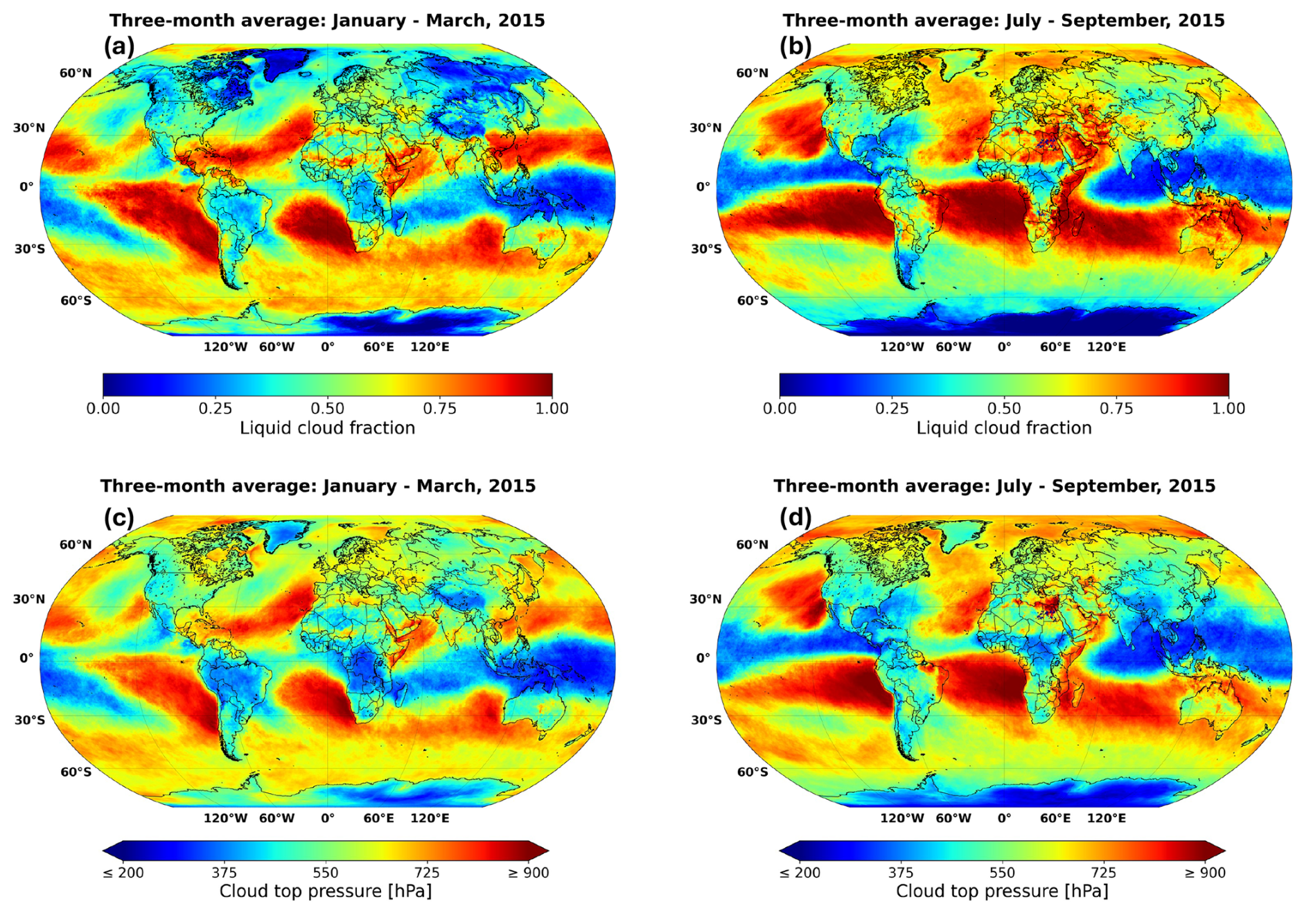
Figure D1 Three-month means for the liquid cloud fractions (LCF) between (a) January–March 2015 and (b) July–September 2015. Panels (c) and (d) represent the same time periods as (a) and (b) respectively, but for the three-month means of the cloud top pressure (CTP) in hPa.